Spatial Locality and Granularity Change in Caching

Abstract

Caches exploit temporal and spatial locality to allow a small memory to provide fast access to data stored in large, slow memory. The temporal aspect of locality is extremely well studied and understood, but the spatial aspect much less so. We seek to gain an increased understanding of spatial locality by defining and studying the Granularity-Change Caching Problem. This problem modifies the traditional caching setup by grouping data items into blocks, such that a cache can choose any subset of a block to load for the same cost as loading any individual item in the block.

We show that modeling such spatial locality significantly changes the caching problem. This begins with a proof that Granularity-Change Caching is NP-Complete in the offline setting, even when all items have unit size and all blocks have unit load cost. In the online setting, we show a lower bound for competitive ratios of deterministic policies that is significantly worse than traditional caching. Moreover, we present a deterministic replacement policy called Item-Block Layered Partitioning and show that it obtains a competitive ratio close to that lower bound. Moreover, our bounds reveal a new issue arising in the Granularity-Change Caching Problem, where the choice of offline cache size affects the competitiveness of different online algorithms relative to one another. To deal with this issue, we extend a prior (temporal) locality model to account for spatial locality, and provide a general lower bound in addition to an upper bound for Item-Block Layered Partitioning.

1 Introduction

A common feature of computer systems is that block granularity changes at different levels of the memory/storage hierarchy. This paper presents the first study of how granularity change affects caching. We define the Granularity-Change (GC) Caching Problem, prove new adversarial competitive bounds for the problem, develop an online GC caching policy with a better competitive ratio than traditional cache policies in this setting, define a new locality model for the problem, and prove upper and lower bounds within this locality model.

Why does block granularity change?

Given that a large and fast memory does not exist, real systems make use of a hierarchy ranging from small, fast memories to larger and slower storage devices [19], typically structured as a hierarchy of caches. Cache hierarchies provide the illusion of a large, fast memory by exploiting temporal and spatial locality in data accesses. Temporal locality refers to when the same data item is referenced multiple times in quick succession. Spatial locality refers to when nearby data items are referenced in quick succession.

Each level of the storage hierarchy organizes its data in blocks to simplify management and reduce overheads. For example, SRAM caches typically consist of 64 B “lines”, DRAM of 2-4 KB “rows”, and flash/disk of 4 KB “pages”. Organizing data in blocks is a simple way for caches to exploit spatial locality, as each block can typically hold multiple data items.

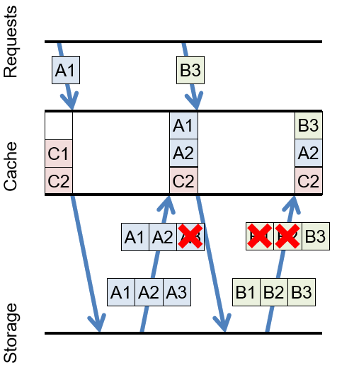
Figure 1: In the GC Caching Problem, caches can load any subset of the larger-granularity block from the level below them, for the same cost. Here, although only A1 is requested, the cache loads the subset {A1,A2} of the block {A1,A2,A3}.

Most caches today ignore granularity change and only load data of their own granularity. But this misses an optimization opportunity to load some or all of the larger-granularity block at minimal cost (see Figure 1), as the lower level has already fetched the entire block. Motivated by this observation, we ask: What caching opportunities and challenges are introduced by granularity change?

What does prior caching work say about block granularity?

The original caching problem is well studied and understood. Belady [7] and Mattson [24] separately devised optimal solutions for caching with unit-size, unit-cost items. Sleator and Tarjan [31] provided both lower and upper bounds for the cost ratio when comparing the performance of online caches, which must make decisions as requests arrive, against offline caches, which are allowed to view the entire trace when making decisions. Fiat et al. [17] extended this work to randomized algorithms and showed ways of approximating online policies using other online policies.

Other variants of caching have been considered, and considerable work has been done on complexity and algorithms for these variants [13, 2, 6, 10, 36, 15]. Caching with variable-size items [14, 8, 37] appears to be similar to GC Caching, since one could think of different subsets of a block as differently sized items. The critical difference is that, unlike in variable-size caching, items in a block can be accessed, cached, and evicted individually.

In GC Caching, choosing which items to load is an additional dimension with significant impact on performance. To our knowledge, there is no prior theoretical work that accounts for the granularity change optimization discussed above. Prior caching work focuses on the temporal locality of items within the access trace (where an item can be of fixed or variable size), and misses the significant impact of spatial locality among data items in the level below. Models of computation that account for transfers to and from the cache in “blocks” (e.g., the External Memory model [1], the Ideal Cache model [18], the Multicore-Cache model [9], and the Parallel Memory Hierarchy model [4]) permit items in a block to be individually accessed from cache, but not individually cached or evicted. As such, the “blocks” are the (smaller) granularity of the cache itself (e.g., A1 in Figure 1) and not the (larger) granularity of the level below (A1 A2 A3), as in our model.

The systems community uses several approaches to handle granularity change. There is work on scheduling memory controllers at granularity boundaries [16, 26, 27, 39, 40, 41], address mapping techniques [33, 23, 38, 35], row-buffer management [25, 28, 32, 34], and item-to-block allocation [11, 12, 5, 29]. Recently, DRAM caches account for granularity change by taking some or all of the larger-granularity block into the smaller-granularity cache on loads [30, 22, 21]. We provide the first theoretical framework to better understand and guide these designs.

Contributions.

We investigate the effects of granularity change on caching. Our results include:

1. We develop a model for caching at a granularity boundary, called the Granularity-Change Caching Problem;

2. We show that Offline GC Caching is NP-Complete;

3. We provide a lower bound on the competitive ratio of deterministic replacement policies in GC Caching;

4. We design and analyze Item-Block Layered Partitioning, a practical GC caching policy, and we prove an upper bound that is much tighter than any policy that considers only a single granularity (Table 1 highlights our bounds);

5. We discuss a new issue that arises in GC Caching where the choice of offline cache size affects the competitiveness of different online algorithms relative to one another, and we develop a locality model for GC Caching that admits upper and lower bounds for fault rate based solely on the system’s cache size and the workload.

2 The Model

The Granularity-Change Caching Model consists of a single level of memory (cache) that receives a series of requests, referred to as accesses, to data items. If the item is in the cache, then the request is served and the cache is not charged. If the item is not in the cache, then the cache must load the item from the subsequent level of memory or storage. If this load causes the amount of data in cache to exceed the cache size $k$, then items must be evicted from the cache to remedy the situation.

What makes the Granularity-Change Caching Model unique is that the universe of items is partitioned into blocks of up to $B{}$ items, such that the cache can load any subset of the items in a block for unit cost; i.e., items after the first are “free” ($B{}$=3 in Figure 1). When each item is in a different block, this model exactly matches the traditional caching model.

The blocks represent the larger data granularity used by the subsequent level of the memory hierarchy. In such systems, there is typically a small memory buffer used to handle data as it is being read or written. The cost of moving data from the subsequent level into this buffer is typically large relative to the cost of operating on the buffer itself. Hence, once items are brought into the buffer, they can be accessed at low cost, motivating our model [19, 20].

Definition 1.

In the Granularity-Change Caching Problem, we are given (i) a cache of size $k$, (ii) an (online or offline) trace $\sigma$ of requests to items, and (iii) a partitioning of the items into disjoint blocks (sets) such that no partition contains more than $B{}$ items. Starting with an empty cache, the goal is to minimize the number of times that an item is not present in the cache when requested in $\sigma$. When a requested item is not in cache, any subset of that item’s block can be loaded, so long as the subset contains the item.

Setting	Sleator-Tarjan Bound	Our GC Lower Bound	Our GC Upper Bound
Constant Augmentation	$k=2h\Rightarrow 2\,\times$	$k\approx 2h\Rightarrow B{}\,\times$	$k\approx 2h\Rightarrow 2B{}\,\times$
Ratio = Augmentation	$k=2h\Rightarrow 2\,\times$	$k\approx{}\sqrt{B{}}h\Rightarrow\sqrt{B}\,\times$	$k\approx{}\sqrt{2B{}}h\Rightarrow\sqrt{2B}\,\times$
Constant Ratio	$k=2h\Rightarrow 2\,\times$	$k\approx{}B{}h\Rightarrow 2\,\times$	$k\approx{}B{}h\Rightarrow 3\,\times$

Table 1: Salient bounds for online cache size $k$ and optimal cache size $h$, shown as: Augmentation $\Rightarrow$ Competitive Ratio. Compared to traditional caching (Sleator-Tarjan Bound), the spatial locality in GC Caching adds a penalty of $\Theta{}(B{})\times{}$ to the product of competitive ratio $\times$ augmentation.

Locality vs. traditional caching models.

In traditional caching models, all hits come from temporal locality, i.e., when an item remains in cache between subsequent accesses. In GC Caching, hits can also come from spatial locality, i.e., when an item $I$ is in cache due to an earlier access to a different item in the same block. (Any hits to item $I$ beyond the first are due to temporal locality, since $I$ would have been brought in cache anyway.)

Assumptions.

We assume that each item has unit size and each block has unit cost. We also assume that the caches we study are much larger than the block size, i.e., $k\gg B{}$. In addition, we limit our results to deterministic policies.

Baseline policies.

We consider two baseline cache designs. An Item Cache loads only the requested item from a block; i.e., it is a traditional cache. By contrast, a Block Cache loads all the items in a requested block and also evicts them together; i.e., it increases the cache’s granularity to operate on blocks instead of items. Item Caches perform well on temporal locality and poorly on spatial locality, whereas Block Caches are the opposite.

Locality Model.

To expand our analysis beyond competitive ratios on cost, we extend the locality of reference model by Albers, Favrholdt, and Giel [3] to account for block granularity. Their model adds a function $f(n)$ (which will increasing and concave for real traces) that characterizes the maximum size of a working set (the number of distinct items accessed) in a window of $n$ accesses across a trace. They use this model to provide bounds on the fault rate (the number of faults per access) of various replacement policies as a function of $f(n)$.

We extend this model to account for block granularity by adding a similar function $g(n)$ to account for the number of distinct blocks accessed in a window of size $n$. The value of $g(n)$ can range from $f(n)$ when each item comes from a different block to $f(n)/B{}$ when entire blocks are accessed at a time. The ratio $f(n)/g(n)$ measures how much spatial locality occurs in a given trace. With this extended model, we can provide bounds on the fault rate of policies in the Granularity-Change Caching Problem.

3 Complexity Analysis

In this section, we investigate the complexity of GC Caching. Using a reduction from variable-size caching, we are able to show that the Offline GC Caching is NP-Complete, even with unit block cost and unit item size.

Theorem 1.

The Offline Granularity-Change Caching Problem is NP-Complete.

Proof.

Our proof relies on a reduction from variable size caching, which is known to be NP-complete [14]. We begin by showing how to create items for the GC Caching Problem and then assign them to blocks. We then use these blocks to generate a trace where the cost paid by the optimal cache is the same as the optimal cost for the variable-size caching problem.

The first step of the reduction is to scale the variable-size caching problem to have integral item sizes. This can be done by multiplying the size of each item and the cache size by the same value (assuming the sizes are rational numbers). After the sizes are all integral, the items of the GC Caching Problem can be created and partitioned. For each item in the variable-size caching problem, we create one block in GC Caching. The maximum size of these blocks can be chosen to be any value greater than or equal to the size of the largest item in the scaled variable-size problem. For each of these blocks we will use only the first $z$ items, where $z$ is the size of the corresponding item in the scaled problem. We refer to these as the active set for that block.

The idea for trace generation is to create a trace for GC Caching that has accesses to the same amount of cache space as in the variable-size problem. For each access in the variable size trace, the GC Caching trace replaces it with consecutive accesses to the active set of the corresponding block. Each item is accessed a number of times equal to the number of items in the active set, in round robin order. The ordering of the variable-size trace is maintained, so that the ordering of the blocks in the GC Caching trace is the same as the ordering of the items in the variable-size trace. The cache size is set to be the same as that of the scaled variable-size problem.

We are left to show that the optimal cost of the GC Caching Problem that we generate is the same as the optimal cost of the variable-size caching problem. First, we show that scaling sizes does not affect the result. Since the cache size was scaled by the same factor as the items, the fraction of the cache space that each item takes remains unchanged.

Beyond this, we show that there is an optimal solution for the generated GC Caching instance that loads and evicts the entire active set of a block at the same time. To do this, we rely on the fact that an optimal solution can load all items from the active set that are not in cache for unit cost. This means that any consecutive series of requests to a single block can be served for that unit cost. However, unless the cache contains the entire active set, it must pay at least unit cost to serve the block.

Since the active sets corresponding to different items in the variable size problem are in distinct blocks, there is no way to load an active item without paying unit cost for that block. When combined with the fact that the active items remain unchanged for each block, we can show that evicting a single active item increases the cost paid by the cache the same as evicting all active items for that block.

If we assume the cache evicts all active items for a block at the same time, then upon the first consecutive access to a block, either the entire active set will be in cache or none of it will be. If the set is in cache, no loads are required. Otherwise, loading less than the entire set will cause the need for additional loads. In particular, the maximum amount of cache space used for the active set multiplied by the number of loads must exceed the active set.

We use the repeated accesses to the active set to show that the benefits of such additional loads cannot outweigh the drawbacks. Since any item can be loaded for unit cost, the benefit of using less cache space for one set of consecutive accesses to the active set cannot exceed the amount of cache space reserved. Due to the repeated nature of the accesses, loading less than the entire active set will result in at least as many additional loads as the size of the active set. This means that loading the entire active set upon the first miss is optimal.

Since we have shown that an optimal solution is to load and evict entire active sets at a time, any access that immediately follows an access to the same active set will automatically be a hit. Putting these results together, the optimal solution to the generated trace is the same as the optimal solution to the original trace. ∎

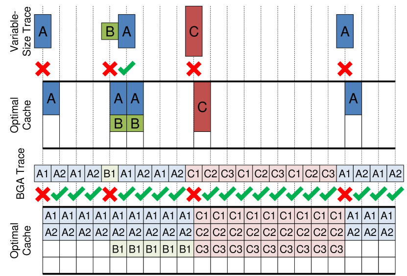
Figure 2: A diagram showing how to transform an instance of variable-size caching into an instance of the GC Caching with the same cost. Notice that storing item A1 with block C would not decrease the number of misses, since A2 would still suffer a miss. The repeated accesses force the optimal solution to load the entire block in order to minimize misses.

Figure 2 shows an example of the reduction. We simulate variable size items through the use of multiple items from the same block accessed consecutively. By repeating these access sequences, we force the optimal solution to load all items that are used in the block. The optimal solution to the input instance can easily be translated into an optimal solution to the generated instance.

4 Competitive Lower Bound

We next show how to adapt prior techniques for competitive ratios to the GC Caching Problem. We will start by providing a lower bound for Item Caches and Block Caches, and then use the insights we gain to devise a more general lower bound.

4.1 Item Caches

We start by examining how Item Caches perform in the GC Caching Problem. These policies are widespread and well studied, so they serve as a logical starting point for our investigation.

The traditional lower bound for Item Caches comes from Sleator and Tarjan [31], and is defined as follows. We define $k$ to be the size of the online cache and $h$ to be the size of the optimal cache.

1. Assume both the optimal and online caches are full.

2. Access $k-h+1$ items that have not been seen before.

3. Create a set of items containing the items in the optimal cache during step one and the items accessed during step two. This set contains $k+1$ items.

4. Access the item from the set that is not in the online cache. Repeat this process a total of $h-1$ times.

5. To generate a longer trace, return to step one. Note that the assumption will be satisfied.

In these traces the online policy never hits, as the items in step two are newly accessed and the items in step four are chosen to be outside of that cache. The optimal policy also misses on every access in step two. Since it knows the future accesses, it can perform evictions so as to store each item that will be accessed in step four, allowing it to achieve hits on all of these accesses.

The GC Caching Problem problem modifies traditional caching by introducing spatial locality. This means that the optimal policy can miss on only one out of every $B{}$ accesses in step two if the items are chosen such that an entire block is accessed. The cost of this modification is that the optimal cache uses $B{}$ space rather than unit space in step two, and thus step four must be shortened to $h-B{}$ accessses. This provides the following result:

Theorem 2.

Any Item Cache has a competitive ratio of at least $B{}(k-B{}+1)/(k-h+1)$ where $k$ is the size of the online cache and $h$ is the size of the optimal cache.

Proof.

Create a trace according to the following procedure. Steps (1), (3), and (5) are the same as above for traditional caching. The other two steps are modified slightly:

• Choose a block that has not been seen before. Access each item from that block. Repeat this process until $k-h+1$ items have been accessed in this step.

• Access the item from the set that is not in the online cache. Repeat this process a total of $h-B{}$ times.

Since the online policy does not load any item that is not accessed, it will miss on each access in step two. The accesses in step four are chosen to ensure that the online policy misses on each.

The optimal policy will load each block on its first access in step two, resulting in $(k-h+1)/B{}$ misses. It can use its remaining $h-B{}$ space to store the items accessed in step four, hitting on each.

Taking the ratio of these misses provides the bound. ∎

This competitive ratio is nearly a multiplicative $B{}$ factor worse than traditional lower bounds under the assumption that $k\gg B{}$. Since the behavior of the policieshas not changed, this shows the increased power of the optimal algorithm in this model.

4.2 Block Caches

If Item Caches do not perform well in the GC Caching Problem, perhaps Block Caches will. They are naturally suited to handle the access sequences Item Caches suffered on, and may therefore offer a better realization of the potential performance improvements.

This intuition proves accurate for the trace design scheme described in Section 4.1, Online Block Caches will be able to hit on all subsequent accesses to a block in step two, providing the same number of misses as the optimal policy on that step. As long as the number of accesses in the second step dominates the number in the third, these policies will perform well.

The problem with Block Caches is that when only a few items of a block are accessed, the remaining items will pollute the cache, reducing the available space to serve accessed items. In particular, when only one item from a block is used at a time, the cache is effectively $B{}$ times smaller. We can apply this insight along with the traditional bound to provide a bound for Block Caches.

Theorem 3.

Any Block Cache has a competitive ratio of at least $k/(k-B{}(h-1))$ where $k$ is the size of the online cache and $h$ is the size of the optimal cache.

Proof.

Create a trace according to the following procedure:

1. Assume both the optimal and online caches are full and that each item in the optimal cache is from a different block.

2. Access one item from each of $\lceil{}k/B{}\rceil{}-h+1$ blocks that have not yet been accessed.

3. Create a set of items containing the items in the optimal cache during step one and the items accessed during step two. This set contains $\lceil{}k/B{}\rceil{}+1$ items, each of which are from a different block.

4. Access the item from the set that is not in the online cache. Repeat this process a total of $h-1$ times.

5. To generate a longer trace, return to step one. Note that the assumption will be satisfied.

The online policy has not seen any of the blocks accessed in step two, so it will miss on each access. Because it loads and evicts at block granularity, it will store exactly $\lceil{}k/B{}\rceil{}$ blocks at a time. This means that step four can always choose one item that is not in the online cache, resulting in misses for all accesses in that step.

The optimal policy will miss on each access in step two for $\lceil{}k/B{}\rceil{}-h+1$ misses. Since it knows what will be accessed in step four, it can choose to keep those items and hit on each such access.

With the assumption that $B{}$ evenly divides $k$, taking the ratio of the misses and simplifying results in the target bound. ∎

This result shows that Block Caches perform very poorly on traces that do not take advantage of the spatial locality that is available in the GC Caching Problem. In particular, they suffer a performance penalty where the effective cache size is reduced by a factor equal to the ratio between the size of the block and the average number of items used per block. This means that the competitive ratio of such policies is infinite unless they have at least $B{}$ times as much space as the optimal policy to which they are being compared.

4.3 Generalizing the Lower Bound

Building on the above discussion, we now provide a more general lower bound for policies beyond Item Caches and Block Caches.

Like the worst-case traces for Item Caches and Block Caches, we will first access new items until the online cache can no longer store the entire active set, and then repeatedly access whichever item the cache chooses not to store. Unlike the previous bounds, we cannot make assumptions about the granularity of loads or evictions.

When adding new items to the active set, we take advantage of spatial locality to allow the optimal cache to outperform the online cache. For any block, the worst-case trace can continue to access an item from that block that is not in the online cache until no such item exists. The online cache will miss on each access, while the optimal cache can load each accessed item on the first access to the block. Using this insight, we categorize policies using a parameter $a{}$, which is the number of distinct consecutive accesses to a block before the policy loads the entire block.

Our trace construction follows what we use for Item Caches, except that the online policy will incur $a{}$ misses on each block in step two and the optimal policy will need to use $a{}$ space to service these requests, leaving only $h-a{}$ space available for step three.

Theorem 4.

For any deterministic replacement policy that requires $a{}$ consecutive distinct accesses to a block to load all of it, the competitive ratio of that policy is at least $(a{}(k-h+1)+B{}(h-a{}))/(k-h+1)$ where $k$ is the size of the online cache and $h$ is the size of the optimal cache.

Proof.

Create a trace according to the following procedure:

1. Assume both the optimal and online caches are full.

2. For $\lceil{}(k-h+1)/B{}\rceil{}$ blocks that have not yet been accessed:
   While there exists an item from that block that the online cache has not yet loaded, access that item. This will occur $a{}$ times per block.

3. Create a set of items containing the items in the optimal cache during step one and the items in the blocks accessed during step two. This set contains at least $k+1$ items.

4. Access an item from the set that is not in the online cache. Repeat this process a total of $h-a{}$ times.

5. To generate a longer trace, return to step one. Note that the assumption will be satisfied.

As with our other traces, the online policy will miss on every access, causeing $a{}\lceil{}(k-h+1)/B{}\rceil{}$ misses in step two and $h-a{}$ in step four. The optimal policy will load each of the $a{}$ items that will be accessed in a block on its first access in step two, resulting in $\lceil{}(k-h+1)/B{}\rceil{}$ misses. It can use its remaining $h-a{}$ space to store the items that will be accessed in step four, hitting on each.

With the assumption that $B{}$ evenly divides $k-h+1$, taking the ratio of the misses and simplifying results in the target bound. ∎

4.4 Analysis and Discussion

Having devised lower bounds for deterministic policies for the GC Caching Problem, we can use the insights we have developed to learn more about the original problem.

Designing Policies.

In order to minimize the lower bound, we need to consider the $a{}$ parameter. In Theorem 4, the $a{}$ parameter shows up in one positive term and one negative term, both in the numerator. When $k-h+1>B{}$, then the positive term dominates, and minimizing $a{}$ also minimizes the competitive ratio. Otherwise, the negative term dominates and maximizing $a{}$ minimizes the ratio. Thus, to achieve the best competitive ratio, one should load either an entire block or a single item, and nothing in between.

This result is true even when we allow the $a{}$ parameter to be non-constant. To show this, we first consider a single cycle of the trace. The online policy suffers misses equal to the sum of its chosen $a{}$ parameters across each block accessed. The optimal cache will use space equal to the maximum number of accesses for a single block to suffer one miss per block. Since this space is forced to store particular items, it cannot be used in step four of the generation, and thus the online policy will suffer that many fewer misses. By applying these observations, we see that the resulting ratio is minimized when $a{}$ is either maximized or minimized.

Since items in a block can only be distinguished by whether they have been accessed or not, it makes sense to either want to bring in all of them or none of them after an access. However, it is less clear why an approach similar to that of the ski-rental problem, where the policy waits for confirmation that additional accesses are coming before incurring the expense of loading the block, is not correct. There appears to be a two-part answer to this question. The first part is the fact that the number of possible “rentals” is bounded by $B{}$. The second is that that the decision to “purchase” additional items is relatively low cost, in that it can easily be changed by evicting the loaded items when a different block is accessed.

The intuition for choosing between 1 and $B{}$ for the $a{}$ parameter can be found in the relative costs due to the types of locality. For caches where the online and offline caches are roughly equal size, the online cache needs as much space as possible to compete on traditional worst-case traces, and using cache space to serve spatial locality is more harmful than helpful. By contrast, when the online cache is much larger than the offline cache, the marginal benefit of the extra lines is small, making them more useful when devoted to handling spatial locality. In these situations, policies that load the entire block on access perform better.

We can apply a similar logic when analyzing eviction. The lower bound for Block Caches shows that evicting at the block granularity is inefficient. We need some way to choose between items in a block for eviction. By considering whether an item has been accessed, we can differentiate items into two classes, preferring items that have been accessed over those that have not.

Putting this all together, we see that in order to maximize performance, policies should load the entire block on an access (unless comparing against an optimal with similar size, where they should load individual items) to take advantage of spatial locality, but evict items individually to give preference to ones that have been accessed over those that have not.

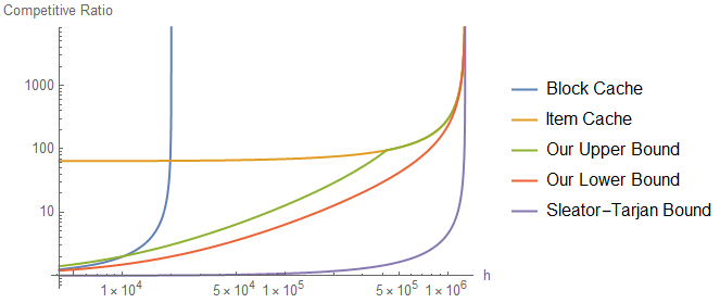
Figure 3: Comparing bounds in the GC Caching Problem. The $x$-axis is the optimal cache size $h$, and the $y$-axis is the competitive ratio. Online cache size $k=1.28M$ and block size $B{}=64$.

The Bound in Context.

Figure 3 plots the competitive ratio bounds, for a fixed online cache size $k=1.28M$ and block size $B=64$. Our resulting lower bound is much greater than the Sleator-Tarjan [31] bound, meaning that the gap between online and offline policies is larger in GC Caching than in traditional caching. The gap starts at a multiplicative factor of nearly $B{}$$\times$ when $k\approx{}h$ (since the $B{}h$ term dominates), and tapers off, hitting $2\times$ when $k\approx{}B{}h$. Table 1 gives three salient points of comparison for the Sleator-Tarjan bound, our lower bound, and our upper bound (discussed in Section 5): constant factor augmentation, the point where the augmentation meets the competitive ratio, and constant competitive ratio. These results show that, compared to traditional caching, the introduction of spatial locality increases the gap between online and offline policies by $B{}\times$, which can be spread between the competitive ratio and the augmentation factor. In prior models, the augmentation factor ($k/h$) equals the competitive ratio when both are $2$. By contrast, in the GC Caching Problem, $k=2h$ has a competitive ratio of $\approx 2+B{}$ and a competitive ratio of $2$ requires $k\approx B{}h$. The meeting point of the augmentation factor and the competitive ratio occurs when $k\approx\sqrt{B{}}h$.

5 Competitive Upper Bound

5.1 Policy Description

Figure 4: A logical diagram of IBLP, consisting of an Item Cache partition running LRU in front of a Block Cache partition running LRU.

Our policy, known as Item-Block Layered Partitioning (IBLP), divides the available space into two layers of cache (Figure 4). The first layer, which serves each access to the cache, loads only the items that are accessed and evicts using the Least-Recently Used (LRU) replacement policy. The second layer, which only serves accesses that miss in the first layer, also uses the LRU policy for evictions, but loads and evicts at the granularity of entire blocks at a time. In other words, IBLP organizes the cache as an Item Cache backed by a Block Cache. We refer to these layers as the item layer and block layer, respectively, and define their sizes as $i{}$ and $b{}$.

Although this is relatively straightforward to describe and implement, it includes some subtle design choices. The cache is split into two different layers to handle the two types of locality, with the item layer handling temporal locality and the block layer handling spatial locality. The ordering of the two layers is important to ensure that accesses with high temporal locality do not reorder blocks in the LRU list of the block layer. Allowing such reorderings would cause blocks with a small number of frequently accessed items to pollute the block layer, reducing its effective space for worst-case traces. Note that the block layer is neither inclusive nor exclusive of the item layer. If the block layer were inclusive of the item layer, the item layer would not contribute to the overall hit rate. By contrast, an exclusive policy would avoid duplicating items, but would require a more complicated method of tracking items to ensure none are evicted before their lifetimes expire in both partitions. Even with our simpler policy, choosing partition sizes is involved. We build up to it by analyzing each layer individually and then combining the analyses, with the results discussed in Section 5.3.

5.2 The Upper Bound

In order to prove our upper bound on the competitive ratio of IBLP, we introduce a new linear programming technique to analyze how the optimal cache makes use of cache space. Using this technique, we will first consider how each layer performs separately against adversarial approaches to the type of locality that it targets. We will then provide an analysis of the combined problem to ultimately prove the upper bound.

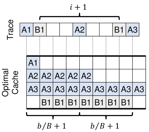
Figure 5: The pattern of accesses resulting in worst-case traces and the resulting cache space used in the optimal cache over time. The accesses to A show the worst-case spatial locality, while the accesses to B show the worst-case temporal locality.

Our Analysis Technique.

Our analysis visualizes the optimal cache’s performance on a trace as a rectangle, with one axis representing the time in units of accesses, and the other representing cache space. When an item is brought into cache, it take up one unit of space and a number of units of time equal to the number of accesses between when it is loaded and when it is evicted. A visualization of this method can be found in Figure 5.

In this method, we assume that each access is chosen so as to cause the online policy that we compare against to miss. Therefore, if we choose a window of time that accurately captures the average long-term behavior of the trace, then the miss ratio is the number of accesses in the window $w$ divided by the difference between that number and the number of hits $o$ the optimal cache can achieve in the window ($w/(w-o))$. We will normalize our result to a window of unit size and consider the hit rate of the optimal cache.

There are two constraints that limit the number of hits the optimal cache can achieve. The first constraint is that of cache usage. This means that the total number of units of space used by the optimal cache cannot exceed the area of the rectangle. To reduce clutter, we will ignore the need to leave one unit of cache space available for accesses that the optimal cache misses on in this analysis. The second constraint is that of accesses. This means that the number of accesses that occur cannot exceed the number of accesses in the window. We will make these constraints more concrete in the analyses below.

Both of these constraints are necessary to fully specify the problem, but they still provide the optimal cache degrees of freedom that are not available in the original GC caching problem. The constraints limit the total amount of the resource (cache usage or accesses) used, but not where these resources are located. This allows the optimal cache to make use of solutions that are not viable in the original caching problem by having multiple accesses occur at the same time or overdrawing cache space at one time in exchange for underutilizing it at a different time. Since this looseness empowers the optimal cache, it can only hurt the resulting bounds.

Temporal Locality.

We begin our analysis by comparing how the item layer and the optimal cache perform on adversarial temporal locality. More specifically, we ignore any hits caused by spatial locality. In this setting, an access can be a miss for the item layer and a hit for the optimal cache if and only if there have been at least $i{}$ distinct items accessed since the item was last accessed. This means that any such hit requires at least $i{}$ units of cache space. Each time this occurs, the access that hits is constrained to be to the same item as the access that caused the load. The accesses to block B in Figure 5 illustrate this pattern.

Turning these constraints into a linear program and solving it provides an upper bound for the competitive ratio of the item layer on temporal locality.

Theorem 5.

When considering hits due to only temporal locality, the item layer of IBLP has a competitive ratio upper bounded by $\frac{i{}}{i-h}$ where $i{}$ is the size of the item layer cache and $h$ is the size of the optimal cache.

Proof.

We define $r$ to be the fraction of accesses that the optimal cache hits on due to temporal locality. The competitive ratio is $\frac{1}{1-r}$. Since there is $h$ cache space in the rectangle and each hit requires $i{}$ cache space, the cache space constraint is $h\geq{}ri{}$. Since each hit forces one access to a particular item, the accesses constraint says that the number of hits must be less than the number of accesses, ie $1\geq r$. Although in this problem, this constraint is loose, it becomes critical for later versions that include spatial locality.

This results in the following linear program:

$$\text{Maximize:\;}\frac{1}{1-r}$$

subject to:

$$h\geq{}ri{}$$

$$1\geq r$$

$$\text{where }r\text{ is the free variable.}$$

Solving this linear program provides the desired result. ∎

This result matches the upper bound from Sleator and Tarjan [31] for traditional LRU caches. Since we are focusing only on temporal locality, this behavior is to be expected, as the item layer behaves exactly like an LRU cache of size $i{}$.

Spatial Locality.

We next consider how the block layer compares to the optimal cache in the face of adversarial spatial locality. Similar to the analysis above, we will ignore any hits not due to our chosen form of locality. However, spatial locality introduces several important variations.

For spatial locality, hits to an item cannot be caused by previous accesses to that item, only misses to a different item in their block that causes the original item to be loaded. This means that each item can cause at most one hit per time that it is loaded. Furthermore, since the number of items loaded at a time is upper bounded by the block size and one of them is the item that was just missed on, the maximum number of hits that can be caused by each miss is at most $B{}-1$.

We now consider what adversarial spatial locality looks like for the block layer. In order for the block layer to miss on an access, there must have been $b{}/B{}$ distinct other blocks accessed since the last access to that block. This means that in order for the optimal cache to achieve multiple hits from the same load operation, each additional item loaded must be stored in cache for $b{}/B+1{}$ accesses more than the previous item. This results in a triangle-like cache usage pattern, as shown for the A block in Figure 5.

The dimensions of this pattern provide an interesting set of tradeoffs. Since the optimal cache must miss at least once in order to load items to hit on, the competitive ratio is upper bounded by the number of items loaded at a time. However, the cache usage of each item increases with the number of items loaded.

The design of the linear program is based on the number of items $t$ that optimal cache chooses to load on each miss and the number of misses $s$ that cause the optimal cache to perform loads. The optimal cache achieves $s(t-1)$ hits, resulting in a competitive ratio of $\frac{1}{1-s(t-1)}$. Since the total cache usage due to each miss is $\sum_{i=0}^{t-1}1+t(b{}/B{}+1)$, the cache usage constraint says that $h\geq{}s(\sum_{i=0}^{t-1}1+t(b{}/B{}+1))$. Similarly, the accesses constraint is $1\geq st$ since each load causes the specific miss and each subsequent hit to be fixed accesses. Solving the resulting linear program provides the resulting bound.

Theorem 6.

When considering hits due to only spatial locality, the block layer of IBLP has a competitive ratio upper bounded by $\text{min}\Big{(}B{},(b{}+2B{}h-B{})/(b{}+B{})\Big{)}$ where $b{}$ is the size of the block layer cache and $h$ is the size of the optimal cache.

Proof.

We define $s$ to be the fraction of accesses where the optimal cache misses and performs loads and $t$ to be the number of items that the optimal cache chooses to load on each miss. The optimal cache achieves $s(t-1)$ hits, resulting in a competitive ratio of $\frac{1}{1-s(t-1)}$. Since the total cache usage due to each miss is $\sum_{i=0}^{t-1}1+t(b{}/B{}+1)$, the cache usage constraint says that $h\geq{}s(\sum_{i=0}^{t-1}1+t(b{}/B{}+1))$. Similarly, the accesses constraint is $1\geq st$ since each load causes the specific miss and each subsequent hit to be fixed accesses. This results in the following maximization problem:

$$\text{Maximize:\;}\frac{1}{1-s(t-1)}$$

subject to:

$$h\geq{}s\Big{(}\sum_{i=0}^{t-1}1+t(b{}/B{}+1)\Big{)}$$

$$1\geq st$$

$$\text{where }s\text{ and }t\text{ are the free variables.}$$

Solving this maximization problem provides the second term in the theorem. The first term comes from the fact that $t$ cannot exceed $B{}$ combined with the second constraint in the linear program. ∎

Combining Temporal and Spatial Locality.

We now show how to combine the two methods of achieving hits to obtain an upper bound for the entirety of IBLP for general traces. Since IBLP hits on an access if either of its partitions hits on that access, the restrictions on an access in order for it to be a miss for IBLP must be stricter. This allows us to formulate a linear program for the entire policy by combining the hits and the constraints of the previous two versions.

The resulting linear program is too complex to solve directly. To deal with this, we modify the spatial locality problem to take the number of hits due to temporal locality as an input. We then use the result of this problem to choose the number of temporal locality hits that maximizes the competitive ratio. The result of this is shown below in Theorem 7.

Theorem 7.

The competitive ratio of IBLP is upper bounded by:

$$\begin{cases}\frac{(b{}+B{}(2i-1))^{2}}{8B{}(B{}+b{})(i{}-h)}&i{}\leq{}\frac{2B{}b-b{}+2B{}^{2}+B{}}{2B{}}\\ \frac{2B{}i{}-B{}b{}+b{}-B{}^{2}-B{}}{2i{}-2h}&i{}>\frac{2B{}b-b{}+2B{}^{2}+B{}}{2B{}}\end{cases}$$

where $i{}\geq h$ is the size of the item layer, $b{}$ is the size of the block layer, and $h$ is the size of the optimal cache.

Proof.

As in the previous proofs, we define $r$, $s$, and $t$ to be the fraction of accesses that the optimal cache hits on due to temporal locality, the fraction of accesses that the optimal cache misses on and loads items for spatial locality, and the number of items loaded for spatial locality, respectively.

The total number of hits that optimal cache achieves is equal to the sum of the hits from the individual localities. This results in a competitive ratio of $\frac{1}{1-r-s(t-1)}$. We combine the amount of cache space used and the number of accesses forced in a similar way. This results in the following linear program:

$$\text{Maximize:\;}\frac{1}{1-r-s(t-1)}$$

subject to:

$$h\geq{}ri{}+s\Big{(}\sum_{i=0}^{t-1}1+t(b{}/B{}+1)\Big{)}$$

$$1\geq r+st$$

$$\text{where }r\text{, }s\text{, and }t\text{ are the free variables.}$$

Unfortunately, we were unable to solve this linear program directly (one hour of computation time in Wolfram Mathematica). To obtain a solution, we break the program into smaller chunks that can be solved individually. We start by modifying the linear program to compute the values of $s$ and $t$ that maximize the competitive ratio given a particular $r$ value. This results in the following values for $s$ and $t$:

$$s=\frac{(B{}+b{})(1-r)^{2}}{b{}-b{}r+B{}(2h-1+r-2i{}r)}$$

$$t=\frac{b{}-b{}r+B{}(2h-1+r-2i{}r)}{(B{}+b{})(1-r)}$$

When we plug in these values and solve the resulting maximization problem, we achieve results for both $r$ and the competitive ratio:

$$r=\frac{b{}+B{}(4h-2i{}-1)}{b{}+B{}(2i{}-1)}$$

$$\text{Ratio}=\frac{(b{}+B{}(2i-1))^{2}}{8B{}(B{}+b{})(i{}-h)}$$

This result is a valid upper bound, but fails to account for the constraint that $t$ cannot exceed the block size $B{}$. By using the expressions for the values of $r$ and $t$, we find that this occurs when $i{}>\frac{2B{}b-b{}+2B{}^{2}+B{}}{2B{}}$. In this region, we know from above that $t$ maxes out at $B{}$. We apply this change to the prior analysis, with the following results:

$$r=\frac{2B{}h-B{}b{}+b{}-B{}^{2}-B{}}{2B{}i{}-B{}b{}+b{}-B{}^{2}-B{}}$$

$$\text{Ratio}=\frac{2B{}i{}-B{}b{}+b{}-B{}^{2}-B{}}{2i{}-2h}$$

Putting these results together finishes the proof. ∎

5.3 Applying the Bound

Having proved a bound on the competitive ratio for IBLP as a function of the layer sizes, we can can now consider how to partition the cache space. This task is complicated by the fact that the optimal partitioning depends on the size of the optimal cache being compared against.

Known optimal size.

When the size of the optimal cache is known, the optimal layer sizes can be directly computed. When $k\geq(3B{}h-h-B{}^{2}-B{})/(B{}-1)$, this results in:

$$\text{Ratio}=\frac{(k+B{}-1)(k-h+B{}(2h-1))}{(k-h+B{})^{2}}$$

$$i=\frac{k^{2}+4B{}hk-hk+4B{}^{2}h-3B{}h-B{}^{2}}{2B{}k+k+2B{}h-h+2B{}^{2}-3B{}}$$

For smaller $k$ values, setting $i=k$ (i.e., operating as an Item Cache) provides the minimum competitive ratio of:

$$\frac{2B{}k-B{}^{2}-B{}}{2(k-h)}$$

This transition occurs at the point where the competitive ratio due to temporal locality exceeds the maximum competitive ratio that can be achieved due to spatial locality ($B{}\times$). In other words, for small $k$ values (relative to $h$), temporal locality dominates performance.

Again considering large caches with large blocks ($k>h\gg B{}\gg 1)$, we see that the ratio is roughly $\frac{k(k+2B{}h)}{(k-h)^{2}}$ if $k\geq{}3h$ and $\frac{B{}k}{k-h}$ if $k<3h$.

Figure 3 shows how this upper bound compares to the lower bound, as well as single-granularity caches of the same size running LRU. IBLP outperforms the small-granularity Item Cache for $k\approx{}3h$ and larger, and it outperforms the large-granularity Block Cache for $k\approx{}4B{}h$ and smaller. In addition, IBLP performs close to optimal for all values of $k$, whereas the performance of the baselines degrades severely outside of their ideal performance conditions.

Table 1 shows how this bound compares to traditional caching and our lower bound. Our upper bound has roughly the same penalty to augmentation and competitive ratio as our lower bound, differing by at most a multiplicative factor of $3\times$. Comparing against the points of interest from the lower bound, we see that the competitive ratio is $\approx 2B{}$ when $k=2h$, $k\approx B{}h$ yields a competitive ratio of $\approx 3$, and the meeting point occurs when $k\approx\sqrt{2B{}}h$.

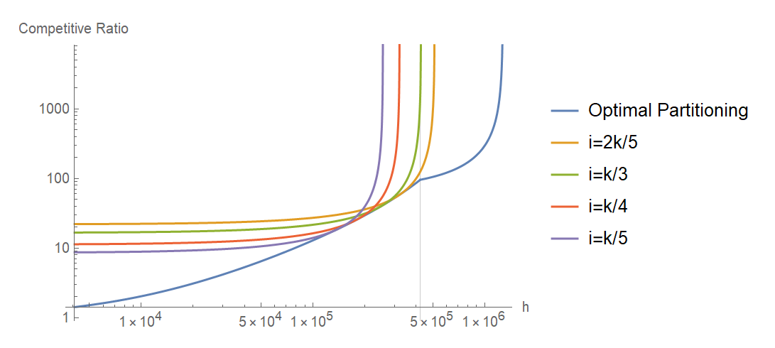
Figure 6: A graph showing how the upper bound of IBLP with constant layer sizes performs compared to the optimal layer sizes. The x-axis is the size of the optimal cache and the y-axis is the competitive ratio (lower is better). In this graph, the online cache size $k=1.28M$ and block size $B{}=64$.

Unknown optimal size.

The optimal layer sizes in IBLP depend on the size of the optimal cache $h$ being compared against. For any fixed layer sizes, the competitive ratio will be optimal at only one value of $h$, but show significant degradation for larger $h$ and limited improvement for smaller $h$ (see Figure 6).

This dependency on the size of the optimal cache is unique amongst known caching problems. Unlike other caching problems, the competitive ratios due to temporal locality and spatial locality are different functions of the optimal cache size. As a result, the relative performance of traces changes depending on optimal cache size, which results in different values of $h$ having different worst-case traces. This suggests that a full understanding of the GC Caching Problem requires analysis beyond competitive ratios.

6 Analysis of Randomized Algorithms

Our previous analysis showed that the relative competitiveness of different replacement policies may depend on the size of the policy compared against. This is undesirable, since we would like to be able to compare policies without relying on a hypothetical comparison point. In this section, we explore the randomized replacement policies in the GC Caching Problem. One would hope that randomized policies, which have can more easily compare against Unfortunately, this hope proves false; we are not able to eliminate the impact of comparison size on relative competitiveness.

6.1 A Randomized Policy

We design a randomized policy by extending the ideas of marking algorithms to the GC Caching Problem. As with traditional marking algorithms, items can be either marked or unmarked. We mark items when they are requested. Evictions must choose from unmarked items, unless all items are marked, in which case all marks are removed and then an item is evicted at random.

Our policy, known as Granularity-Change Marking (GCM for short), accounts for granularity change by loading each item in the accessed block, but not marking them. This results in a system where items that show spatial but not temporal locality are loaded into cache but do not result in the eviction of items with temporal locality. In the special (but common) case where the number of unmarked items in the cache is smaller than the block size but greater than zero, the requested item is loaded and then the remaining unmarked items in cache are replaced by randomly selected items from the accessed block.

We will briefly compare GCM with similar policies that make different choices for handling granularity change. First, we compare to a marking algorithm that ignores granularity change. It is easy to show that this policy has a competitive ratio of at least $B{}$ regardless of size (as long as the optimal cacheis $B{}$ or larger) by repeatedly choosing a new block and accessing each item in it. This shows the importance of loading additional items from the requested block. However, a policy that loads and marks every item in the block also has issues. In particular, like the analysis of Block Caches in Section 4.2, when the trace does not provide spatial locality, the effective size of the cache is reduced by the excess items. Unlike the deterministic setting, there may be value in a policy that loads some but not all of the items in the accessed block. However, due to the issues with competitive ratios in this setting, we did not pursue this analysis in detail.

6.2 Analyzing Relative Competitiveness

We now show that randomized algorithms in the GC Caching Problem do not bypass the issue where their relative competitiveness may depend on the size of the cache compared against. In particular we continue to have the issue where policies must decide how many items to load on each access. Similar to the above analysis, caches that load few items perform well compared to optimal caches of similar size, when each line devoted to temporal locality matters significantly. However, this hinders their performance when compared against optimal caches of significantly smaller size, where spatial locality becomes more important. Caches that load many items on each access suffer from the opposite set of tradeoffs. This relative change is not affected by randomness, leaving our issue unresolved.

7 Beyond Competitive Ratios

We would like to be able to use the GC Caching Problem to design and analyze caches independent of a hypothetical comparator. However, competitive ratios seem to require this knowledge to provide insight into policy performance. To remedy this, we turn to the locality of reference model discussed in Section 2. In this model, the functions $f(n)$ and $g(n)$ provide bounds on the number of items and blocks, respectively, seen in a window of $n$ accesses. We use these functions to provide bounds on the fault rates of deterministic policies in the GC Caching Problem.

7.1 Lower Bound

The addition of spatial locality in the GC Caching means that the lower bound on fault rates in the traditional locality of reference model does not apply. We provide a lower bound for deterministic policies in this new model.

Theorem 8.

Any deterministic replacement policy has a fault rate of at least:

$$\frac{g(f^{-1}(k+1)-2)}{f^{-1}(k+1)-2}$$

where $k$ is the size of the cache.

Proof.

Following the ideas of Albers et al. [3], we will construct a family of traces such that for any $n$, there exists a trace of length $n$ in the family where the policy will have a fault rate no lower than the bound. We construct traces in our family using $k+1$ distinct items. Due to the locality constraints, these items can be partitioned into at most $g(f^{-1}(k+1)-2)$ blocks. We generate traces in phases, where each phase consists of $f^{-1}(k+1)-2$ accesses divided into $k-1$ repetitions. A repetition consists of repeated accesses to a single item that has not yet been accessed this phase. In each phase, repetition $1\leq{}j\leq{}k-1$ starts with the $f^{-1}(j+1)-1$th access of that phase and continues until the access before the next block starts. We can apply the techniques of Albers et al. [3] to show that these traces are consistent with $f(n)$.

It remains to discuss $g(n)$ and show the minimum fault rate of policies on these traces. In the work of Albers et al. [3], the item chosen is the one of the $k+1$ used in the trace that is not in the cache, and therefore every repetition causes one miss. However, in our model, our ability to choose items is limited by the $g(n)$ function. In particular, the item not in cache may be from a block that has not been accessed yet in the phase. If this is the case, then choosing that item increases the number of blocks accessed in the window, which may cause a violation. However, it is known that a new block can be chosen at least $g(p)$ times for a phase of length $p$. Each of these new block choices returns us the freedom to guarantee that we can pick the item that is not in cache. ∎

7.2 Upper Bound

We now provide an upper bound for the fault rate of IBLP. Since this policy consists of two layers of cache acting in concert, both layers must miss in order for the entire cache to miss. We therefore begin by providing bounds for both layers individually.

Theorem 9.

The fault rate of the item layer of IBLP is at most:

$$\frac{i{}-1}{f^{-1}(i{}+1)-2}$$

where $i{}$ is the size of the item layer.

Proof.

The item layer is simply an LRU cache that operates as though it were in the traditional model. The change in model cannot cause the fault rate to increase, since it only introduces new ways for a policy to hit. This means that we can rely on the result from Albers et al. [3] on bounds on LRU policies in the traditional model. Plugging in the size of the item layer as the cache size to this provides our result. ∎

The upper bound for the fault rate of the block layer requires a slight transformation before relying on the same straightforward application of the traditional bound.

Theorem 10.

The fault rate of the block layer of IBLP is at most:

$$\frac{b{}/B{}-1}{f^{-1}(b{}/B{}+1)-2}$$

where $i{}$ is the size of the item layer.

Proof.

The block layer is a Block Cache, meaning that it loads and evicts at the granularity of blocks. Thus, the behavior of the block layer depends on the block that is accessed, but is independent of the particular item. We can combine these facts to view the block layer as an LRU cache with effective size $b{}/B{}$ serving a trace where requests are to blocks. Substituting in the effective size of the cache and using the number of blocks in a window $g(n)$ as the items per window function, we achieve the resulting bound. ∎

Taking the minimum of these fault rates for a given input provides an upper bound on the fault rate of IBLP.

Theorem 11.

The fault rate of IBLP with item layer size $i{}$ and block layer size $b{}$ is upper bounded by:

$$\min{}\left(\frac{i{}-1}{f^{-1}(i{}+1)-2},\frac{b{}/B{}-1}{f^{-1}(b{}/B{}+1)-2}\right)$$

where $f(n)$ is a function mapping a window size to the maximum number of items accessed in a window of size $n$ and $f(n)$ is a function mapping a window size to the maximum number of items accessed in a window of size $n$.

f(n)	g(n)	Lower Bound	item layer UB	block layer UB
$x^{1/2}$	$x^{1/2}$	$1/h$	$1/i{}$	$B{}/b{}$
$x^{1/2}$	$x^{1/2}/B^{1/2}$	$1/(B^{1/2}h)$	$1/i{}$	$1/b{}$
$x^{1/2}$	$x^{1/2}/B{}$	$1/B{}h$	$1/i{}$	$1/B{}b{}$
$x^{1/p}$	$x^{1/p}$	$1/h^{p-1}$	$1/i^{p-1}$	$B^{p-1}/b^{p-1}$
$x^{1/p}$	$x^{1/p}/B^{1/2}$	$1/(B^{(p-1)/p}h^{p-1})$	$1/i^{p-1}$	$1/b^{p-1}$
$x^{1/p}$	$x^{1/p}/B{}$	$1/B{}h^{p-1}$	$1/i^{p-1}$	$1/B{}b^{p-1}$

Table 2: Salient bounds for comparing an equally split cache ($i{}=b{}$) to the lower bound for a cache of half the size ($h=i+b{}$).

7.3 Analysis

We have provided a method for analyzing the performance IBLP or other policies in the GC Caching that does not rely on the existence of a hypothetical optimal comparison point. We now show how to apply this analysis. To do this, we will analyze IBLP with equal partition sizes ($i{}=b{}$).

For this analysis, we will consider polynomial locality functions (i.e., $f^{-1}(n)=cn^{p}$ for some real numbers $c$ and $p$). Since locality functions must be positive concave functions, this covers the majority of high order terms that would occur in real traces. Exponential functions are also possible, but such functions signify an extremely high degree of locality, where even small, simple caches should perform well. We will compare our result with the lower bound for a cache of the same size as each partition, which provides a result roughly equivalent to competitive ratio with an augmentation factor of $2\times$ (i.e., $i{}+b{}=k=2h$).

When $f(n)=g(n)$, there is no spatial locality. In this situation, the upper bound for the Item Cache matches the lower bound of the baseline, while the Block Cache will be off by a factor of $B{}^{p-1}$ (recall that $p$ is the degree of the high order term of $f(n)$). With maximum spatial locality, $f(n)=B{}g(n)$. In this situation, the upper bound for the Block Cache matches the lower bound of the baseline, while the Item Cache will be off by a factor of $B{}$. The largest gap between the baseline and the upper bound for IBLP occurs when the ratio between $f(n)$ and $g(n)$ is $B^{1-(1/p)}$. This represents input with very high, but not maximal, spatial locality. For input with this locality, the upper bounds for both partitions meet at $1/i^{p-1}$. This ends up differing from the baseline by a factor equal to the ratio of $f(n)$ and $g(n)$, $B^{1-(1/p)}$. As the value of $p$ approaches $\infty$, this gap approaches $B{}$.

There are two primary takeaways from this analysis. The first is that the two methods of analysis are in agreement, as our competitive ratio results also show a ratio of $B{}$ for an augmentation factor of 2. The second is that the performance of IBLP is worst when locality is high (large $p$ implies high temporal locality and large ratios of $f(n)$ and $g(n)$ implies high spatial locality). When locality is so high, our miss rate will be very low. Therefore, the relatively large multiplicative factor gap will result in a small number of additive misses. This suggests that IBLP will perform well in practice.

8 Conclusion

In this work, we have provided a theoretical foundation for the study of spatial locality in caching. We started with a traditional treatment of the new GC Caching Problem, showcasing the changes caused by spatial locality through proving an NP-completeness result for the offline problem and new lower bounds on competitive ratios. We used the insights gained from these works to develop IBLP and provide strong, provable bounds for its performance. Our upper bound illustrates how competitive ratios become a flawed metric in the GC Caching Problem due to a dependency on the size of the hypothetical comparison point. We solve this problem by extending a locality of reference model to the GC Caching Problem, and provide analysis of IBLP in this new model.

Acknowledgments.

Supported in part by NSF grants CCF-1919223, CCF-2028949, a Google Research Scholar Award, a VMware University Research Fund Award, and by the Parallel Data Lab (PDL) Consortium.

References

- [1] A. Aggarwal and J. S. Vitter. The Input/Output complexity of sorting and related problems. Commun. ACM, 31(9), 1988.
- [2] S. Albers, S. Arora, and S. Khanna. Page replacement for general caching problems. In SODA, 1999.
- [3] S. Albers, L. M. Favrholdt, and O. Giel. On paging with locality of reference. Journal of Computer and System Sciences, 70(2):145–175, 2005.
- [4] B. Alpern, L. Carter, and J. Ferrante. Modeling parallel computers as memory hierarchies. In Programming Models for Massively Parallel Computers, 1993.
- [5] H. Attiya and G. Yavneh. Remote memory references at block granularity. In OPODIS, 2017.
- [6] A. Bar-Noy, R. Bar-Yehuda, A. Freund, J. Naor, and B. Schieber. A unified approach to approximating resource allocation and scheduling. JACM, 2001.
- [7] L. A. Belady. A study of replacement algorithms for a virtual-storage computer. IBM Systems journal, 1966.
- [8] D. S. Berger, N. Beckmann, and M. Harchol-Balter. Practical bounds on optimal caching with variable object sizes. In SIGMETRICS, 2018.
- [9] G. E. Blelloch, R. A. Chowdhury, P. B. Gibbons, V. Ramachandran, S. Chen, and M. Kozuch. Provably good multicore cache performance for divide-and-conquer algorithms. In SODA, 2008.
- [10] M. Brehob, S. Wagner, E. Torng, and R. Enbody. Optimal replacement is np-hard for nonstandard caches. IEEE Transactions on Computers, 2004.
- [11] B. Calder, C. Krintz, S. John, and T. Austin. Cache-conscious data placement. In ASPLOS, 1998.
- [12] T. M. Chilimbi, M. D. Hill, and J. R. Larus. Cache-conscious structure layout. In PLDI, 1999.
- [13] M. Chrobak, H. J. Karloff, T. H. Payne, and S. Vishwanathan. New results on server problems. SIAM Journal on Discrete Mathematics, 1991.
- [14] M. Chrobak, G. J. Woeginger, K. Makino, and H. Xu. Caching is hard-even in the fault model. Algorithmica, 2012.
- [15] G. Even, M. Medina, and D. Rawitz. Online generalized caching with varying weights and costs. In SPAA, 2018.
- [16] X. Fan, C. Ellis, and A. Lebeck. Memory controller policies for dram power management. In ISLPED, 2001.
- [17] A. Fiat, R. M. Karp, M. Luby, L. A. McGeoch, D. D. Sleator, and N. E. Young. Competitive paging algorithms. Journal of Algorithms, 1991.
- [18] M. Frigo, C. E. Leiserson, H. Prokop, and S. Ramachandran. Cache-oblivious algorithms. In FOCS, pages 285–298, 1999.
- [19] J. L. Hennessy and D. A. Patterson. Computer architecture: a quantitative approach. 2011.
- [20] B. Jacob, D. Wang, and S. Ng. Memory systems: cache, DRAM, disk. 2010.
- [21] D. Jevdjic, G. H. Loh, C. Kaynak, and B. Falsafi. Unison cache: A scalable and effective die-stacked dram cache. In MICRO, 2014.
- [22] D. Jevdjic, S. Volos, and B. Falsafi. Die-stacked dram caches for servers: Hit ratio, latency, or bandwidth? have it all with footprint cache. In ISCA, 2013.
- [23] W.-F. Lin, S. K. Reinhardt, and D. Burger. Designing a modern memory hierarchy with hardware prefetching. IEEE Transactions on Computers, 2001.
- [24] R. L. Mattson, J. Gecsei, D. R. Slutz, and I. L. Traiger. Evaluation techniques for storage hierarchies. IBM Systems journal, 1970.
- [25] S. Miura, K. Ayukawa, and T. Watanabe. A dynamic-sdram-mode-control scheme for low-power systems with a 32-bit risc cpu. In ISLPED, 2001.
- [26] O. Mutlu and T. Moscibroda. Stall-time fair memory access scheduling for chip multiprocessors. In MICRO, 2007.
- [27] O. Mutlu and T. Moscibroda. Parallelism-aware batch scheduling: Enhancing both performance and fairness of shared dram systems. In ISCA, 2008.
- [28] S.-I. Park and I.-C. Park. History-based memory mode prediction for improving memory performance. In ISCAS., 2003.
- [29] E. Petrank and D. Rawitz. The hardness of cache conscious data placement. In POPL, 2002.
- [30] M. K. Qureshi and G. H. Loh. Fundamental latency trade-off in architecting dram caches: Outperforming impractical sram-tags with a simple and practical design. In MICRO, 2012.
- [31] D. D. Sleator and R. E. Tarjan. Amortized efficiency of list update and paging rules. Communications of the ACM, 1985.
- [32] V. V. Stankovic and N. Z. Milenkovic. DRAM controller with a close-page predictor. In EUROCON, 2005.
- [33] K. Sudan, N. Chatterjee, D. Nellans, M. Awasthi, R. Balasubramonian, and A. Davis. Micro-pages: increasing dram efficiency with locality-aware data placement. In ASPLOS, 2010.
- [34] Y. Xu, A. S. Agarwal, and B. T. Davis. Prediction in dynamic SDRAM controller policies. In SAMOS, 2009.
- [35] H. Yoon, J. Meza, R. Ausavarungnirun, R. A. Harding, and O. Mutlu. Row buffer locality aware caching policies for hybrid memories. In ICCD, 2012.
- [36] N. Young. The k-server dual and loose competitiveness for paging. Algorithmica, 1994.
- [37] N. E. Young. On-line file caching. Algorithmica, 2002.
- [38] Z. Zhang, Z. Zhu, and X. Zhang. A permutation-based page interleaving scheme to reduce row-buffer conflicts and exploit data locality. In MICRO, 2000.
- [39] H. Zheng, J. Lin, Z. Zhang, E. Gorbatov, H. David, and Z. Zhu. Mini-rank: Adaptive dram architecture for improving memory power efficiency. In MICRO, 2008.
- [40] Z. Zhu and Z. Zhang. A performance comparison of dram memory system optimizations for smt processors. In HPCA, 2005.
- [41] Z. Zhu, Z. Zhang, and X. Zhang. Fine-grain priority scheduling on multi-channel memory systems. In HPCA, 2002.