Early Stage Convergence and Global Convergence of Training Mildly Parameterized Neural Networks

Abstract

The convergence of GD and SGD when training mildly parameterized neural networks starting from random initialization is studied. For a broad range of models and loss functions, including the most commonly used square loss and cross entropy loss, we prove an “early stage convergence” result. We show that the loss is decreased by a significant amount in the early stage of the training, and this decrease is fast. Furthurmore, for exponential type loss functions, and under some assumptions on the training data, we show global convergence of GD. Instead of relying on extreme over-parameterization, our study is based on a microscopic analysis of the activation patterns for the neurons, which helps us derive more powerful lower bounds for the gradient. The results on activation patterns, which we call “neuron partition”, help build intuitions for understanding the behavior of neural networks’ training dynamics, and may be of independent interest.

1 Introduction

As deep learning shows its capability in various fields of applications, extensive researches are done to theoretically understand and explain its great success. Among the topics covered by these theoretical studies, the optimization of deep neural networks is one of the most crucial one, especially given the fact that simple optimization algorithms such as Gradient Descent (GD) and Stochastic Gradient Descent (SGD) can easily achieve zero training loss (47), although the loss landscape of training neural networks is highly non-convex (27; 41). Existing works attempting to answer the surprising convergence ability usually work in settings that do not align well with realistic practices. For example, the notable Neural Tangent Kernel (NTK) theory (20; 17; 16; 3; 50) shows the global convergence of SGD in highly over-parameterized regime, in which the loss landscape is approximated by a quadratic function. In practice, though, the loss landscape is indeed highly non-convex with spurious local minima and saddle points (39; 40), and the dynamics of neurons show nonlinear behaviors (34).

Nevertheless, fast decreasing of the loss value always happens when the network trained is not highly over-parameterized, at least in the early stage of training. It is common that the loss experiences a drastic decreasing at the beginning of the training. In many cases, this decrease of loss even continues until the loss achieves zero, i.e. the optimization algorithm fully converges. In this paper, we study the early stage or full convergence of GD and SGD when under-parameterized or mildly over-parameterized models are trained. Specifically, we answer the following two theoretical questions:

When we train practical-size neural networks by GD or SGD,

1. Does the fast convergence in the early stage of the training provably exist? If so, how

long will the phenomenon last and how much will loss descend in the early stage?

2. Can the global convergence be proved under some special conditions

on loss function and training data?

Our answers to the questions above are roughly summarized in the following main theorems:

Main Theorem 1 (Informal statement of Theorem 4.2 and 4.6).

For mildly over-parameterized or under-parameterized two-layer neural networks with quadratic loss or general classification loss (Assumption 4.4), let parameters be trained by GD or SGD started with random initialization. If the learning rate $\eta\leq 0.01$, then in the first $\Theta(1/\eta)$ iterations, the loss will descend $\Omega(1)$.

Main Theorem 2 (Informal statement of Theorem 5.2 and 5.3).

For mildly over-parameterized or under-parameterized two-layer neural networks with exponential-type loss (Assumption 5.1), let parameters be trained by GD with random initialization and proper learning rate. If data is well-separated (satisfies Assumption 4.1), the loss converges to $0$ at exponential rate or arbitrary polynomial rate, depending on the conditions.

In the first main theorem, we demonstrate that the fast convergence in the early stage of training happens under weak conditions. The model does not need to be highly over-parameterized, and the loss function can take quite general forms. In the second main theorem, we further prove the full convergence of GD for exponential-type loss and well-separated dataset. These assumptions on the loss function and training data are close to practice and widely picked by previous theoretical studies  (22; 23; 38; 8; 7; 32; 33). “Full convergence” means that our analysis covers all the stages of the training process, starting from initialization to the convergence to zero loss. This is different from existing works which focus on the convergence process after the training accuracy hits 100% (32; 23; 8). Moreover, we provide the convergence rate of GD for two classes of neural networks.

During the theoretical analysis, we study the dynamics of neurons in detail and capture the effect of each sample on each neuron. We call our results “neuron partition”, which provides a accurate description to the behavior of neurons. With the neuron partition results, we derive a novel gradient lower bound for mildly parameterized neural networks, which is vital for the convergence results. The neuron partition also provides rich intuition for how the convergence happens. When GD or SGD is used with small initialization, the network is initially close to the saddle point at $0$, which might be hard for GD to escape. However, neurons will adjust their directions rapidly and enter a good region which contains neither spurious local minima nor saddle points. Then, neurons will keep moving through the right directions for $\Theta(1/\eta)$ iterations, during which the loss descends quickly and significantly. For exponential-type loss and well-separated training data, the second stage will proceed uninterruptedly until training is stopped.

2 Related Work

Due to the highly non-convex loss landscape (27; 41), classical optimization theories such as convex optimization fail to characterize the convergence of training neural networks. Researchers have proposed theories specifically for neural networks. We list some below.

A popular line of works focus on the highly over-parameterized neural networks and derive the “Neural tanget kernel (NTK)” theory. In the NTK regime (20; 17; 16; 2; 3; 4; 5; 14; 50; 28; 11; 18; 19), the neural network model is close to a kernel method, leading to the nearly convex optimization landscape. Global convergence is proven in this regime. Besides, for highly over-parameterized neural networks, the mean-field approach (10; 36; 37) is another line, which analyze the training dynamics by Wasserstein gradient flow.

However, the NTK regime is different from real practical neural networks in several aspects. First, practical neural networks are often mildly over-parameterized rather than highly over-parameterized (31). Second, the landscape for practical neural networks is usually more complicated, containing local minima and saddle points (39; 40; 15). Finally, the empirical superiority of neural networks over kernel methods is obvious. For example, neural networks can learn single neuron efficiently (45; 43), while kernel methods fail unless the network size is exponentially large with respect to the input dimension (46).

Furthermore, optimization theories for neural networks beyond the NTK regime has also been studied. (39; 15) proved that spurious local minima are common in the loss landscape. (40) pointed out that neither one-point convexity nor Polyak-Łojasiewicz condition holds near the global minimum. In (32; 23; 8; 7; 49), local convergence results are given with cross-entropy loss or some special networks at the late stage of training, i.e. when training loss is small enough. In (30; 38; 33; 21; 9), global convergence results are given for some special networks, special data distribution or special target functions.

3 Preliminaries

3.1 Notations

We use bold letters for vectors or matrices and lowercase letters for scalars, e.g. $\boldsymbol{x}=(x_{1},\cdots,x_{d})^{\top}\in\mathbb{R}^{d}$ and $\mathbf{P}=(P_{ij})_{m_{1}\times m_{2}}\in\mathbb{R}^{m_{1}\times m_{2}}$. We use $\left<\cdot,\cdot\right>$ for the standard Euclidean inner product between two vectors, and $\left\|\cdot\right\|$ for the $l_{2}$ norm of a vector or the spectral norm of a matrix. We use $a\lesssim b$ to indicate that there exists an absolute constant $c>0$ such that $a\leq cb$, and $a\gtrsim b$ is similarly defined. We use standard progressive representation $\mathcal{O},\Omega,\Theta$ to hide absolute constants. For any positive integer $n$, let $[n]=\{1,\cdots,n\}$. Denote by $\mathcal{N}(\boldsymbol{\mu},\mathbf{\Sigma})$ the Gaussian distribution with mean $\boldsymbol{\mu}$ and covariance matrix $\mathbf{\Sigma}$, $\mathbb{U}(S)$ the uniform distribution on a set $S$. Denote by $\mathbb{I}\{E\}$ the indicator function for an event $E$. For a square matrix $P$, we use $\lambda_{\min}(\mathbf{P})$ to denote its smallest singular value.

3.2 Problem settings

In this paper, we consider supervised learning problems. Let $\mathcal{P}$ be a data distribution on $\mathbb{R}^{d}\times\mathbb{R}^{C}$. We are given $n$ training data $\mathcal{S}=\{(\boldsymbol{x}_{i},\boldsymbol{y}_{i})\}_{i=1}^{n}\subset\mathbb{R}^{d}\times\mathbb{R}^{C}$ drawn i.i.d. from $\mathcal{P}$. Without loss of generality, we assume $\left\|\boldsymbol{x}\right\|\leq 1$ for any $(\boldsymbol{x},\boldsymbol{y})$ sampled from $\mathcal{P}$.

We consider the empirical risk minimization (ERM) problem, which tries to minimize the empirical risk $\mathcal{L}(\cdot)$ with loss function $\ell(\cdot,\cdot)$:

$$\mathcal{L}(\boldsymbol{\theta})=\frac{1}{n}\sum_{i=1}^{n}\ell(\boldsymbol{y}_{i},\boldsymbol{f}(\boldsymbol{x}_{i};\boldsymbol{\theta})),$$ (1)

where $\boldsymbol{f}(\boldsymbol{x};\boldsymbol{\theta})\in\mathbb{R}^{C}$ is the model and $\boldsymbol{\theta}$ represents all parameters of the model. We will give specific forms to the loss function and the model in the analysis in later sections.

We use Gradient Descent (GD) or Stochastic Gradient Descent (SGD) starting from random initialization to solve the ERM problem. The update rules of GD or batch SGD can be written as:

$${\rm\textbf{GD}}:\quad\boldsymbol{\theta}(t+1)=\boldsymbol{\theta}(t)-\eta_{t}\nabla\mathcal{L}(\boldsymbol{\theta}(t)),$$ (2)

$${\rm\textbf{SGD}}:\quad\boldsymbol{\theta}(t+1)=\boldsymbol{\theta}(t)-\frac{\eta_{t}}{B}\sum_{i\in\mathcal{B}_{t}}\nabla\ell(\boldsymbol{y}_{i},f(\boldsymbol{x}_{i};\boldsymbol{\theta}(t))),$$ (3)

where $\mathcal{B}_{t}=\{\gamma_{t,1},\cdots,\gamma_{t,B}\}$ is a batch, and $\gamma_{t,1},\cdots,\gamma_{t,B}\overset{\text{i.i.d.}}{\sim}\mathbb{U}([n])$ and are independent with $\boldsymbol{\theta}(t)$. The random initialization will be specified in each theorem.

4 Early Stage Convergence

In this section, we state and discuss our main results on the fast convergence in the early stage of training. The models we focus on are mildly over-parameterized or under-parameterized neural networks. As a warm up, in Section 4.1, we study a simple case with binary classification problems and quadratic loss. Then, in Section 4.2, we extend our results to multi-class classification problems with general loss and one-hot labels. We provide discussions to our results in Section 4.3.

4.1 Binary classification with quadratic loss

In this subsection, we study the ERM problem (1) with quadratic loss $\ell(y_{1},y_{2})=\frac{1}{2}(y_{1}-y_{2})^{2}$ and the two-layer ReLU neural network model without bias:

$$f(\boldsymbol{x};\boldsymbol{\theta})=\sum_{k=1}^{m}a_{k}\sigma(\boldsymbol{b}_{k}^{\top}\boldsymbol{x}),$$ (4)

where $\sigma(z)=\text{ReLU}(z)$, $\boldsymbol{\theta}=(a_{1},\cdots,a_{m},\boldsymbol{b}_{1}^{\top},\cdots,\boldsymbol{b}_{m}^{\top})^{\top}\in\mathbb{R}^{dm+m}$. We consider the following random initialization

$$\begin{gathered}a_{k}(0)\overset{\text{i.i.d.}}{\sim}\mathbb{U}(\pm{1}/{\sqrt{m}}),\quad\boldsymbol{b}_{k}(0)\overset{\text{i.i.d.}}{\sim}\mathcal{N}(\mathbf{0},\frac{\kappa^{2}}{md}\mathbf{I}_{d}),\quad\text{for\ }k\in[n],\end{gathered}$$ (5)

where $\kappa$ is a constant that controls the initial scale of the first layer.

We focus on the training data with two classes with good separation given by the following assumption.

Assumption 4.1.

(i) $n$ is even. $y_{i}=1$ for $i\in[n/2]$; $y_{i}=-1$ for $i\in[n]-[n/2]$. $\boldsymbol{x}_{i}^{\top}\boldsymbol{x}_{j}\geq 0$ for $i,j$ in the same class; $\boldsymbol{x}_{i}^{\top}\boldsymbol{x}_{j}\leq 0$ for $i,j$ in different classes. (ii) There exists a constant $\mu_{0}>0$, s.t. $\min\limits_{\{i\in[n],\boldsymbol{v}\in\mathbb{R}^{d}|\boldsymbol{v}^{\top}\boldsymbol{x}_{i}\leq 0\}}\max\limits_{\{j\in[n]|\boldsymbol{v}^{\top}\boldsymbol{x}_{j}>0\}}y_{i}\boldsymbol{x}_{i}^{\top}\boldsymbol{x}_{j}y_{j}\geq\mu_{0}$.

For Assumption 4.1 (i), similar assumption has been used in prior works (38). For image classification problems, this assumption can be ensured by a simple transformation on the data due to the non-negative pixels of images. Specifically, given an image dataset consisted of two classes, we just need to replace $\boldsymbol{x}$ with $-\boldsymbol{x}$ for any $(\boldsymbol{x},y)$ in the second class. Assumption 4.1 (ii) is a technical assumption used in the analysis. It is not a strong addition over Assumption 4.1 (i). For example, if there exists a $(x_{0},y_{0})$ in the dataset $S$ such that $(-x_{0},-y_{0})$ is also in $S$, then the dataset $S$ satisfies Assumption 4.1 (ii) with $\mu_{0}=1$ (the upper bound of $\mu_{0}$ is $1$). Admittedly, this technical assumptions is a limitation of our theory—it restricts its applicability. We will search for the relaxation of this assumption in future works.

Now we state the following result.

Theorem 4.2.

Suppose Assumption 4.1 holds. Let $\boldsymbol{\theta}(t)$ be the parameters of model (4) trained by Gradient Descent (2) with quadratic loss. If the width $m={\Omega}(\log(n/\delta))$, the input dimension $d=\Omega(\log m)$, the learning rate $\eta_{t}=\eta\leq 0.01$ and the initialization scale $\kappa=\mathcal{O}(\eta\mu_{0}/n)$ in (5), then, with probability at least $1-\delta-2me^{-2d}$, the loss will descend ${\Omega}(1)$ in $T=\Theta(\frac{1}{\eta})$ iterations.

From our proof in Appendix A, we have the following corollary with fixed numbers about $\eta,\kappa,m$ instead of progressive expressions.

Corollary 4.3.

Suppose Assumption 4.1 holds. Let $\boldsymbol{\theta}(t)$ be the parameters of model (4) trained by Gradient Descent (2) with quadratic loss. Let $\eta=\boldsymbol{0.01}$, $\kappa\leq\min\{\eta/{2000},{\eta\mu_{0}}/{3n}\}$, $m\geq\max\{144\log(2n^{2}/\delta),4\}$, and $\gamma_{1},\gamma_{2}=\Theta(1)$ be constants related with the data distribution defined in (10) in Appendix A. Then, with probability at least $1-\delta-2me^{-2d}$, in $T=\boldsymbol{44}$ iterations, loss will descend at least $0.193(\gamma_{1}-\gamma_{2}\sqrt{8\log(n^{2}/\delta)/m})-0.0111=\Omega(1-\sqrt{\log(n/\delta)/m})$.

Conclusions in Theorem 4.2 show the meaning of “mildly parameterized” in our title. The network does not need to be over-parameterized, i.e. the number of parameters may be smaller than the number of training data. Hence, we pick the term “mildly parameterized” instead of the more widely use “mildly over-parameterized”. The former is weaker than the latter.

4.2 Multi-class classification with general loss and one-hot labels

In this subsection, we extend the early stage convergence results above to more practical settings. Specifically, we consider classification problem with one-hot labels and the general loss functions that satisfy the following conditions.

Assumption 4.4.

The loss function $\ell(\cdot,\cdot)$ can be expressed as $\ell(\boldsymbol{y}_{1},\boldsymbol{y}_{2})=\tilde{\ell}(\boldsymbol{y}_{1}^{\top}\boldsymbol{y}_{2})$ such that: (i) $\tilde{\ell}(\cdot)$ is twice differentiable in $\mathbb{R}$; (ii) $\tilde{\ell}(\cdot)$ is non-negative and non-increasing in $\mathbb{R}$; (iii) there exist $z_{0}\in(0,1]$, $g_{\min},g_{\max}>0,h_{\max}\geq 0$ such that $g_{\min}\leq-\tilde{\ell}^{\prime}(z)\leq g_{\max}$ and $0\leq\tilde{\ell}^{\prime\prime}(z)\leq h_{\max}$ hold for any $z\in[0,z_{0}]$.

It is easy to verify that exponential loss $\ell(\boldsymbol{y}_{1},\boldsymbol{y}_{2})=e^{-\boldsymbol{y}_{1}^{\top}\boldsymbol{y}_{2}}$ ($z_{0}=1$, $g_{\min}=\frac{1}{e}$, $g_{\max}=1$, $h_{\max}=1$), logistic loss $\ell(\boldsymbol{y}_{1},\boldsymbol{y}_{2})=\log(1+e^{-\boldsymbol{y}_{1}^{\top}\boldsymbol{y}_{2}})$ ($z_{0}=1$, $g_{\min}=\frac{1}{e+1}$, $g_{\max}=\frac{1}{2}$, $h_{\max}=\frac{1}{4}$) and hinge loss $\ell(\boldsymbol{y}_{1},\boldsymbol{y}_{2})=\max\{0,1-\boldsymbol{y}_{1}^{\top}\boldsymbol{y}_{2}\}$ ($z_{0}=1$, $g_{\min}=1$, $g_{\max}=1$, $h_{\max}=0$) all satisfy the conditions in Assumption 4.4.

On the training data, we impose the following assumption, which is milder than Assumption 4.1.

Assumption 4.5.

There exists $s>-1$ s.t. ${\left<\boldsymbol{x}_{i},\boldsymbol{x}_{j}\right>}\geq s$ for any $i,j\in[n]$.

Note that now we do not need any separability of training data, but only require there is no pair of data going into opposite directions. (We can even normalize the data and let $\left\|\boldsymbol{x}\right\|<1-\epsilon$ for some $\epsilon>0$, rather than $\left\|\boldsymbol{x}\right\|\leq 1$. Then, the above assumption naturally holds.) Notably, Assumption 4.5 is more widely applicable than Assumption 4.1 above. It holds for normalized image datasets such as MNIST (26) and CIFAR-10 (24).

For the model, we use the two-layer ReLU neural network model with bias as our prediction model:

$$\boldsymbol{f}(\boldsymbol{x};\boldsymbol{\theta})=\sum_{k=1}^{m}\boldsymbol{a}_{k}\sigma(\boldsymbol{b}_{k}^{\top}\boldsymbol{x}+c_{k}),$$ (6)

where $\sigma(z)=\text{ReLU}(z)$, $\boldsymbol{a}_{k}\in\mathbb{R}^{C}$ and $\boldsymbol{\theta}=(\boldsymbol{a}_{1}^{\top},\cdots,\boldsymbol{a}_{m}^{\top},\boldsymbol{b}_{1}^{\top},\cdots,\boldsymbol{b}_{m}^{\top},c_{1},\cdots,c_{m})^{\top}\in\mathbb{R}^{(d+C+1)m}$. We consider random initialization $\boldsymbol{b}_{k}(0)\overset{\text{i.i.d.}}{\sim}\mathcal{N}(\mathbf{0},\frac{\kappa^{2}}{m(d+1)}\mathbf{I}_{d})$, $c_{k}(0)=\frac{\kappa}{\sqrt{m(d+1)}}$, and $\boldsymbol{a}_{k}(0)=(1/\sqrt{m},\cdots,1/\sqrt{m})^{\top}$ for $k\in[m]$, where $\kappa$ is again a constant that controls the initial scale of the first layer.

We show the following convergence result:

Theorem 4.6.

Under Assumption 4.4 and 4.5, let $\boldsymbol{\theta}(t)$ be the parameters of model (6) trained by Stochastic Gradient Descent (3). If the width $m={\Omega}(1)$, the input dimension $d=\Omega(\log m)$, the batch size $B=\Omega(\log m)$, the learning rate $\eta_{t}=\eta\leq 0.01$ and the initialization scale $\kappa=\mathcal{O}(\eta/B)$, then with probability at least $1-\delta-\mathcal{O}(me^{-d})-\mathcal{O}(m0.17^{B})$, the loss will descend ${\Omega}(1)$ in $T=\Theta(\frac{1}{\eta})$ iterations.

By our analysis in Appendix B, we have the following corollary which gives specific numbers about $\eta,\kappa,m$ instead of progressive expression.

Corollary 4.7.

Under the same assumptions as Theorem 4.6, let $\boldsymbol{\theta}(t)$ be the parameters of the model (6) trained by SGD (3). Let $\eta=\boldsymbol{0.01}$, $\kappa\leq\min\{\eta/10,\eta/3B\}$, $m\geq 6$; $z_{0}=1$, $g_{\min}=\frac{1}{2}$, $g_{\max}=1$, $h_{\max}=1$ (in Assumption 4.4) and $s=0$ (in Assumption 4.5). Then, with probability at least $1-\delta-4me^{-\frac{d+1}{2}}-m0.17^{B}$, in $T=\boldsymbol{34}$ iterations, loss will descend at least $0.262533=\Omega(1)$.

We remark here that the weaker Assumption 4.5 in this subsection compared with the Assumption 4.1 before is made possible by the one-hot labels. For one-hot labels, each label component is non-negative. Hence, neural networks can quickly learn a positive bias, allowing the loss to drop significantly.

4.3 Discussion

A large number of classical convergence analysis focus on the late stage of training. For neural networks’ optimization, many works focus on the period of training after the loss is smaller enough (32; 23; 8; 49). However, the early stage is at least as important as the late stage, especially for non-convex problems.

The theoretical results we present in this section demonstrate the fast convergence during the early stage of optimization, i.e. the (short) period of time after the initialization. The two main results, Theorem 4.2 and 4.6, imply that if we train two-layer neural networks by GD or SGD with learning rate $\eta\leq 0.01$, then the loss will descend significantly ($\Omega(1)$) in the first $T=\Theta(1/\eta)$ iterations.

Our results work under realistic settings. For models, our results hold for mildly over-parameterized and under-parameterized neural networks, because we only need the width $m=\Omega(\log(n/\delta))$. For loss functions, our results apply for practical losses, such as quadratic loss and cross entropy loss. On the algorithm side, the results work for both GD (2) and SGD (3).

Though both concerning convergence of GD and SGD, our results are essentially different from the NTK theory, especially on the requirement of over-parameterization. Our results only need $m=\Omega(\log(n/\delta))$, while in the NTK analysis usually assumes that $m$ is polynomial in $n,1/\kappa$ or etc, excluding the practical settings. Moreover, from the analysis side, we establish fine-grained analysis of the training dynamics of each neuron, which may be of independent interested. See Section 6 for a summary of our techniques, and Appendix A and B for the detailed proof. Our analysis helps understand how the convergence in the early stage happens. When GD or SGD is used with small initialization, the initial network is close to the saddle point at $0$. However, neurons will adjust directions rapidly, and the iterator will enter a good region which contains neither spurious local minima nor saddle points. Then, neurons will keep going towards the right directions for a period of time, during which process the loss will descend fast and significantly.

5 Global Convergence

When stronger conditions are imposed on the data distribution and the loss function, we can show global convergence of GD, i.e. starting from any initialization, the GD descends the loss to 0.

For loss functions, we consider the following exponential-type classification loss:

Assumption 5.1.

The loss function $\ell(\cdot,\cdot)$ can be expressed as $\ell(\boldsymbol{y}_{1},\boldsymbol{y}_{2})=\tilde{\ell}(\boldsymbol{y}_{1}^{\top}\boldsymbol{y}_{2})$ such that: (i) $\tilde{\ell}(\cdot)$ is twice continuously differentiable in $\mathbb{R}$; (ii) $\tilde{\ell}(\cdot)$ is positive and non-increasing in $\mathbb{R}$; (iii) there exist $g_{b}>0,h\geq 0$ s.t. $-\frac{\tilde{\ell}^{\prime}(z)}{\tilde{\ell}(z)}\leq g_{b}$ and $0\leq\frac{\tilde{\ell}^{\prime\prime}(z)}{\tilde{\ell}(z)}\leq h$ for any $z\in\mathbb{R}$; (iv) there exists $g_{a}>0$, s.t. $g_{a}\leq-\frac{\tilde{\ell}^{\prime}(z)}{\tilde{\ell}(z)}$ for any $z\geq 0$.

The similar assumption on exponential-type loss has been used in prior works (32). It is easy to verify that both exponential loss $\ell(\boldsymbol{y}_{1},\boldsymbol{y}_{2})=e^{-\boldsymbol{y}_{1}^{\top}\boldsymbol{y}_{2}}$ ($g_{a}=g_{b}=h=1$) and logistic loss $\ell(\boldsymbol{y}_{1},\boldsymbol{y}_{2})=\log(1+e^{-\boldsymbol{y}_{1}^{\top}\boldsymbol{y}_{2}})$ ($g_{a}=\frac{1}{2}$, $g_{b}=1$, $h=1$) satisfy the conditions in Assumption 5.1.

Let $V$ be a constant defined as

$$V=\frac{1}{16}\Big{(}\frac{1}{2}-\sqrt{\frac{8\log(n^{2}/\delta)}{m}}\Big{)}\max\Big{\{}\frac{2}{n}+\frac{n-2}{n}\gamma,\lambda_{\min}(\mathbf{X}_{+}^{\top}\mathbf{X}_{+})\wedge\lambda_{\min}(\mathbf{X}_{-}^{\top}\mathbf{X}_{-})\Big{\}},$$ (7)

where $\mathbf{X}_{+}:=(\boldsymbol{x}_{1},\cdots,\boldsymbol{x}_{\frac{n}{2}})\in\mathbb{R}^{d\times\frac{n}{2}}$, $\mathbf{X}_{-}:=(\boldsymbol{x}_{\frac{n}{2}+1},\cdots,\boldsymbol{x}_{n})\in\mathbb{R}^{d\times\frac{n}{2}}$, and $\gamma:=\min\limits_{i,j\text{in the same class}}\boldsymbol{x}_{i}^{\top}\boldsymbol{x}_{j}\geq 0$. We have the following convergence theorems in which $V$ controls the convergence speed.

Theorem 5.2.

Under Assumption 5.1 and Assumption 4.1, let $\boldsymbol{\theta}(t)$ be the parameters of model (4) trained by Gradient Descent (2) starting from random initialization (5). Let the width $m={\Omega}(\log(n/\delta))$, the initialization scale $\kappa=\mathcal{O}(\eta_{0}{\mu_{0}}/n)$ in (5), $V$ be defined in (7), $c$ be a constant in $(0,\frac{1}{6(1+2\eta_{0})^{2}+2}]$, the constant $c^{\prime}>0$ be sufficiently small, the hitting time $T_{0}=\lceil(n\log 2)^{\frac{2}{Vc}}\rceil$, the parameter $r\in[1,+\infty)$ and the learning rate satisfy

$$\left\{\begin{array}[]{ll}\eta_{0}\leq 1/2\sqrt{2},&\text{for}\ t=0\\ \eta_{t}=\frac{c}{t\mathcal{L}(\boldsymbol{\theta}(t))},&\text{for}\ 1\leq t<T_{0}\\ \eta_{t}=\frac{c^{\prime}}{\mathcal{L}(\boldsymbol{\theta}(t))^{1-\frac{1}{2r}}},&\text{for}\ t\geq T_{0}\\ \end{array}\right..$$

Then, with probability at least $1-\delta-2me^{-2d}$, GD will converge at polynomial rate:

$$\left\{\begin{array}[]{ll}\mathcal{L}(\boldsymbol{\theta}(t))\leq\frac{\mathcal{L}(\boldsymbol{\theta}(1))}{t^{\frac{Vc}{2}}},&1\leq t<T_{0}\\ \mathcal{L}(\boldsymbol{\theta}(t))=\mathcal{O}\big{(}\frac{1}{t^{r}}\big{)},&t\geq T_{0}\\ \end{array}\right..$$

Theorem 5.3.

Under Assumption 5.1 and Assumption 4.1, let $\{\boldsymbol{b}_{k}(t)\}_{k\in[m]}$ be the input layer parameters of model (4), and we only train this layer by Gradient Descent (2) starting from random initialization (5). Let the width $m={\Omega}(\log(n/\delta))$, the initialization scale $\kappa=\mathcal{O}(\eta_{0}\mu_{0}/n)$ in (5), the constant $V$ be defined in (7), the constant $c\leq\frac{1}{2}$ and the learning rate satisfy

$$\left\{\begin{array}[]{ll}\eta_{0}\leq 1/2\sqrt{2},&\text{for}\ t=0\\ \eta_{t}=\frac{c}{\mathcal{L}(\boldsymbol{\theta}(t))},&\text{for}\ t\geq 1\\ \end{array}\right..$$

Then with probability at least $1-\delta-2me^{-2d}$, GD will converge at exponential rate:

$$\mathcal{L}(\boldsymbol{\theta}(t))\leq\Big{(}1-\frac{Vc}{2}\Big{)}^{t-1}\mathcal{L}(\boldsymbol{\theta}(1)),\quad t\geq 1.$$

Theorem 5.2 and 5.3 describe the whole training process starting from random initialization to convergence. If all parameters in the network are trained, we obtain the global convergence with arbitrary polynomial rate. On the other hand, if only the input layer parameters $\{\boldsymbol{b}_{k}\}_{k\in[m]}$ are trained, we can obtain exponential convergence rate. Fixing some layers of the neural network is a common practice for theoretical studies (8). The results show that adaptively increasing learning rate helps GD achieve faster convergence. Similar idea has been explored in previous works such as (32; 8).

A similar convergence result was proven in (38). where the authors showed a global convergence result of two-layer neural networks trained by Gradient Flow (GF) with cross entropy loss and orthogonal separable data. The main difference between our results and analysis with that in (38) is that we study GD instead of GF. Due to the discretization, GD is more complicated than GF. For example, the balanced property of two layers ($\sum_{k\in[m]}|a_{k}(t)|^{2}-\sum_{k\in[m]}\left\|\boldsymbol{b}_{k}(t)\right\|^{2}\equiv 0,\ \forall t\geq 0$) holds for GF throughout the training, but it does not hold for GD. Dealing with GD requires new analysis techniques and finer analysis, such as the neuron partition results we derive. Another related work is  (25). The neural partition approach in our article shares some similarity with the view of gating networks. In their work, the authors use gating networks to understand the role of depth in training deep ReLU networks. By comparison, we focus more on the characterization of training dynamics of two-layer ReLU networks.

6 Proof Sketch and Techniques

6.1 Main techniques in the proof of Theorem 4.2

Inspired by the empirical work (34), we study the nonlinear behavior of each neuron in the early stage of training. First, we define the hitting time $T$, and we will study the convergence in the early stage $0\leq t\leq T$:

$$T:=\sup\big{\{}t\in\mathbb{N}:\ \max_{i\in[n]}\left|f(\boldsymbol{x}_{i};\boldsymbol{\theta}(s))\right|\leq 1,\ a_{k}(s)a_{k}(0)>0,\ \forall k\in[m],\ \forall 0\leq s\leq t+1\big{\}}.$$

6.1.1 Neuron partition: fine-grained dynamical analysis of each neuron and each sample

During our proof, we conduct fine-grained analysis to the interaction of neurons and samples. Specifically, we characterize the impact of each sample on each neuron, and for each sample classify neurons into four categories according to their effect. We call this analysis “neuron partition”.

For the $i$-th training data $(\boldsymbol{x}_{i},y_{i})$, we divide all neurons into four categories during training 0$\leq t\leq T$ and study them separately. We define the true-living neurons $\mathcal{TL}_{i}(t)$, the true-dead neurons $\mathcal{TD}_{i}(t)$, the false-living neurons $\mathcal{FL}_{i}(t)$ and the false-dead neurons $\mathcal{FD}_{i}(t)$ at time $t$ as:

$$\mathcal{TL}_{i}(t):=\big{\{}k\in[m]:y_{i}a_{k}(t)>0,\boldsymbol{b}_{k}(t)^{\top}\boldsymbol{x}_{i}>0\big{\}},$$

$$\mathcal{TD}_{i}(t):=\big{\{}k\in[m]:y_{i}a_{k}(t)>0,\boldsymbol{b}_{k}(t)^{\top}\boldsymbol{x}_{i}\leq 0\big{\}},$$

$$\mathcal{FL}_{i}(t):=\big{\{}k\in[m]:y_{i}a_{k}(t)<0,\boldsymbol{b}_{k}(t)^{\top}\boldsymbol{x}_{i}>0\big{\}},$$

$$\mathcal{FD}_{i}(t):=\big{\{}k\in[m]:y_{i}a_{k}(t)<0,\boldsymbol{b}_{k}(t)^{\top}\boldsymbol{x}_{i}\leq 0\big{\}}.$$

It is easy to verify $[m]=\mathcal{TL}_{i}(t)\bigcup\mathcal{TD}_{i}(t)\bigcup\mathcal{FL}_{i}(t)\bigcup\mathcal{FD}_{i}(t)$ (see Lemma A.1).

Under a weak assumption on the width of the network, we have the following results for the neuron partition at initialization:

Lemma 6.1 (Informal statement of Lemma A.2).

If $m=\Omega(\log(n/\delta))$, then with high probability, if data $i$ and data $j$ are in the same class, we have $\text{card}\big{(}\mathcal{TL}_{i}(0)\cap\mathcal{TL}_{j}(0)\big{)}\approx\frac{\pi-\arccos(\boldsymbol{x}_{i}^{\top}\boldsymbol{x}_{j})}{4\pi}m$.

The next important lemma characterizes the evolution of the neuron partition under GD dynamics.

Lemma 6.2 (Informal Lemma A.4).

With high probability, for any $i\in[n]$ and $t\leq T$ we have:
(S1) True-living neurons remain true-living: $\mathcal{TL}_{i}(t)\subset\mathcal{TL}_{i}(t+1)$.
(S2) False-dead neurons remain false-dead: $\mathcal{FD}_{i}(t)\subset\mathcal{FD}_{i}(t+1)$.
(S3) True-dead neurons turn true-living in the firt step ($t=0$): $\mathcal{TD}_{i}(0)\subset\mathcal{TL}_{i}(1)$.
(S4) False-living neurons turn false-dead in the firt step ($t=0$): $\mathcal{FL}_{i}(0)\subset\mathcal{FD}_{i}(1)$.
(S5) For any $i\in[n]$, $1\leq t\leq T$, $k\in[m]$ and $\boldsymbol{b}\in\overline{\boldsymbol{b}_{k}(t)\boldsymbol{b}_{k}(t+1)}$, we have $\text{sgn}(\boldsymbol{b}^{\top}\boldsymbol{x}_{i})\equiv\text{sgn}(\boldsymbol{b}_{k}^{\top}(1)\boldsymbol{x}_{i})\neq 0$.

To interpret Lemma 6.2, we display the first-step dynamics in Figure 1.

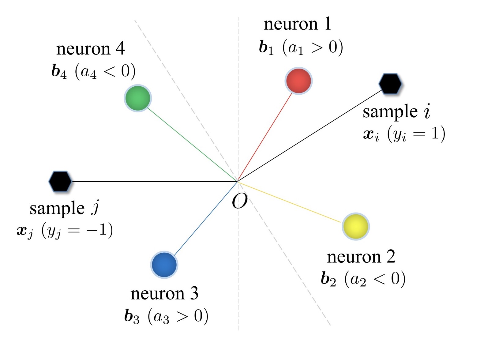
(a) $t=0$.

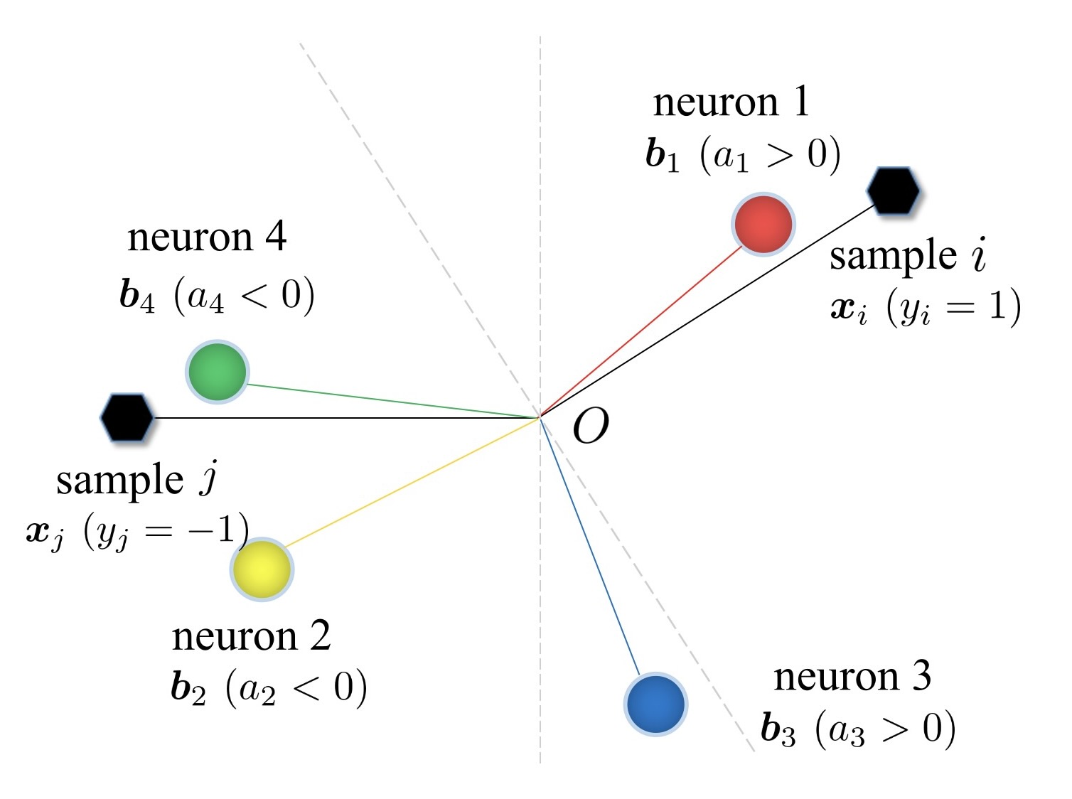
(b) $t=1$.

Figure 1: The first-step dynamics of four neurons which belong to different neuron partitions at $t=0$ for sample $i$ (with label $1$) and sample $j$ (with label $-1$). Fig 1(a) and Fig 1(b) depict the directions of each neuron at $t=0$ and $t=1$, respectively. Results in Lemma 6.2 can be visualized: (S1) neuron $1\in\mathcal{TL}_{i}(0)$ and $1\in\mathcal{TL}_{i}(1)$. (S2) neuron $4\in\mathcal{FD}_{i}(0)$ and $4\in\mathcal{FD}_{i}(1)$. (S3) neuron $2\in\mathcal{TL}_{j}(0)$ and $2\in\mathcal{TL}_{j}(1)$. (S4) neuron $2\in\mathcal{FL}_{i}(0)$ and $2\in\mathcal{FD}_{i}(1)$. (Counterexample) By our Lemma, the first-step dynamics of neuron $3$ cannot happen.

6.1.2 Estimate of hitting time and parameters

Before the analysis of loss descent, we need to estimate the hitting time $T$ and the speed of change for each $a_{k},\boldsymbol{b}_{k}$ in the early stage. Our tool is comparing the hitting time $T$ with an exponentially growing hitting time $T_{e}$ (see (12) in Appendix A).

$$T_{e}:=\sup\Big{\{}t\in\mathbb{N}:\ (1+2\eta)^{2(t+1)}-(1-2\eta)^{2(t+1)}\lesssim 1;\ \ (1+2\eta)^{t+1}\lesssim 1\Big{\}},$$

where the order of magnitude of the two absolute constants hidden by $\lesssim$ is $10^{0}$.

Generally speaking, we can prove the following facts.

Lemma 6.3 (Informal Lemma A.7 and A.8).

For any sample $i\in[n]$ and $t\leq T_{e}$, we have:
(P1) For any $k\in\mathcal{TL}_{i}(t)$, $a_{k}(t)\text{sgn}(a_{k}(0))$ is non-decreasing, and $a_{k}(t)$, $\boldsymbol{b}_{k}(t)$ have an exponential upper bound.
(P2) For any $k\in[m]$, $a_{k}(t)$ has an exponential lower bound.
(P3) $f\big{(}\boldsymbol{x}_{i};\boldsymbol{\theta}(t))$ has an exponential upper bound.
(P4) $T\geq T_{e}\geq T^{*}=\Theta(\frac{1}{\eta})$.

6.1.3 Gram matrix and gradient lower bound

The gradient lower bound is usually an important technical component in the analysis of loss descent. Our analysis establishes a novel lower bound for the gradient for mildly parameterized neural networks based on the neuron partition.

If we define the error for sample $i$ at $t$ as $e_{i}(t)=f(\boldsymbol{x}_{i};\boldsymbol{\theta}(t))-y_{i}$, and the Gram matrix at $t$ as $\mathbf{G}(t)=(\nabla f(\boldsymbol{x}_{i};\boldsymbol{\theta}(t))^{\top}\nabla f(\boldsymbol{x}_{j};\boldsymbol{\theta}(t)))_{(i,j)\in[n]\times[n]}$. For the analysis of GD, loss descent is determined by $\left\|\nabla\mathcal{L}(\boldsymbol{\theta}(t))\right\|^{2}=\sum_{i=1}^{n}\sum_{j=1}^{n}e_{i}(t)\text{G}_{i,j}(t)e_{j}(t)$. Qualitatively, bigger gradient leads to the faster descent of the loss. To derive a tight lower bound for the gradient, we first derive the following bound for the entries of the Gram matrix:

Lemma 6.4 (Informal Lemma A.9).

Under the condition of Theorem 4.2, with high probability, the Gram matrix $\mathbf{G}(t)=\begin{pmatrix}\mathbf{G}_{+}(t)&\mathbf{0}_{\frac{n}{2}\times\frac{n}{2}}\\ \mathbf{0}_{\frac{n}{2}\times\frac{n}{2}}&\mathbf{G}_{-}(t)\end{pmatrix}$ has the following form for any $1\leq t\leq T$ and $i,j\in[\frac{n}{2}]$: $\text{G}_{+}(t)_{i,j},\ \text{G}_{-}(t)_{i,j}\gtrsim\boldsymbol{x}_{i}^{\top}\boldsymbol{x}_{j}\Big{(}\frac{\pi-\arccos(\boldsymbol{x}_{i}^{\top}\boldsymbol{x}_{j})}{4\pi}-\mathcal{O}(\sqrt{\frac{\log(n/\delta)}{m}}\big{)}\Big{)}>0$, where the order of magnitude of the absolute constant hidden by $\gtrsim$ is $10^{0}$.

Combining the estimate above as well as estimates on parameters and the prediction function, we establish our gradient lower bound.

Lemma 6.5 (Informal Lemma A.10).

For any $1\leq t\leq T^{*}$, $\left\|\nabla\mathcal{L}(\boldsymbol{\theta}(t))\right\|=\Omega\big{(}1-(1+2\eta)^{2t}\big{)}$.

Besides, since we consider GD, the following per-step estimate of loss function (6) as well as the Hessian upper bound is also useful.

Lemma 6.6 (Informal Lemma A.11 and A.12).

For $1\leq t\leq T^{*}-1$, we have $H:=\sup\limits_{\boldsymbol{\theta}\text{ along GD trajectory}}\left\|\nabla^{2}\mathcal{L}(\boldsymbol{\theta})\right\|=\mathcal{O}(1)$ and $\mathcal{L}(\boldsymbol{\theta}(t+1))\leq\mathcal{L}(\boldsymbol{\theta}(t))+\left<\nabla\mathcal{L}(\boldsymbol{\theta}(t)),\boldsymbol{\theta}(t+1)-\boldsymbol{\theta}(t)\right>+\frac{1}{2}H\left\|\boldsymbol{\theta}(t+1)-\boldsymbol{\theta}(t)\right\|^{2}$.

6.2 Proof outline of Theorem 4.2

First, we can estimate the initial neuron partition (Lemma 6.1) at the initialization. Then, we study the dynamics of neuron partition trained by GD (Lemma 6.2), which gives a precise directional characterization about each neuron for each sample. Next, by comparing with an exponentially growing hitting time, we can estimate the hitting time $T$ and the parameters (Lemma 6.3). Combining Lemma 6.1, 6.2 and 6.3, we derive a dynamical lower bound of each element of Gram matrix (Lemma 6.4), which induces our gradient lower bound (Lemma 6.5). Finally, by combining the gradient lower bound (Lemma 6.5) and the loss upper bound (Lemma 6.6), we complete our proof. For more details, please refer to Appendix A.

The proof of Theorem 4.6 is similar to Theorem 4.2 and put into Appendix B.

6.3 Proof outline of Theorem 5.2 and 5.3

The proofs of Theorem 5.2 and 5.3 still rely on the dynamical analysis of neuron partition for each sample. First, the estimate of initial neuron partition (Lemma 6.1) also holds, and the dynamical analysis of neuron partition in Lemma 6.2 holds for any $t\geq 1$ (Lemma C.5 and C.6). Second, we can prove that the structure and lower bound of Gram matrix in Lemma 6.4 hold for any $t\geq 1$ (Lemma C.9), which induces the gradient lower bound below. Finally, combining the estimate of gradient lower bound, Hessian upper bound and loss upper bound, we complete our proof. For more details, please refer to Appendix C and D.

Lemma 6.7 (Informal Lemma C.10).

Under the condition of Theorem 5.3, with high probability, we have the following lower bound for any $t\geq 1$: $\left\|\nabla\mathcal{L}(\boldsymbol{\theta}(t))\right\|\gtrsim\mathcal{L}(\boldsymbol{\theta}(t))$, where the absolute constant hidden by $\gtrsim$ is $\sqrt{V}$, defined in (7).

In (32; 8), gradient lower bounds are derived for the late stage of training when $\mathcal{L}(\boldsymbol{\theta}(t))<1/n$, and take the form $\left\|\nabla\mathcal{L}(\boldsymbol{\theta}(t))\right\|\gtrsim\mathcal{L}(\boldsymbol{\theta}(t))\log\big{(}1/\mathcal{L}(\boldsymbol{\theta}(t))\big{)}/\left\|\boldsymbol{\theta}(t)\right\|$. Our lower bound, instead, works on the whole training process. With this stronger gradient lower bound, we can show the exponential convergence in Theorem 5.3.

Another important technical detail is the stability of GD, i.e., the learning rate should be upper bounded by the quantity related with the top eigenvalue of the Hessian. Our analysis also considered this factor, but implicitly. For global convergence results, the loss function we consider is exponential-type, whose Hessian can be controlled by the loss value. For example, for Theorem 5.2, there exists an absolute constant $C>0$, s.t. $\left\|\nabla^{2}\mathcal{L}(\boldsymbol{\theta}(t))\right\|\leq Ct\mathcal{L}(\boldsymbol{\theta}(t))$ for any $t\geq 1$, please refer to Lemma C.15 in the appendix. Therefore, we can transform the Hessian-controlled learning rate condition into the loss-controlled learning rate condition in Theorem 5.2.

7 Experiments

MNIST and CIFAR-10 experiments. As we mentioned in Section 4.2, our theory about early stage convergence applies to a wide range of dataset (Assumption 4.5) such as MNIST and CIFAR-10. We use the two datasets (with normalization) to compare the experimental result with Theorem 4.6. Specifically, we use the first 1000 data in MNIST dataset and the first 1000 data in CIFAR-10 dataset, separately. (The two datasets with normalization $\left\|\boldsymbol{x}\right\|=1$ both satisfy Assumption 4.5.) And we use the two-layer ReLU network with the logistic loss $\ell(\boldsymbol{y}_{1},\boldsymbol{y}_{2})=\log(1+\exp(-\boldsymbol{y}_{1}^{\top}\boldsymbol{y}_{2}))$. $m,\kappa,\eta$ are choosen by Theorem 4.6. We study the change of our bounds under different network width $m$ and learning rate $\eta$. All experiments are conducted on a MacBook pro 13" only using CPU. See the code at https://github.com/wmz9/Early_Stage_Convergence_NeurIPS2022.

Table 1: Results of MNIST and CIFAR-10 experiments. In the first table, we fix $\eta=0.01$ and change $m$; in the second one, we fix $m=200$ and change $\eta$.

$m$	100	200	500	1000
Our hitting iteration	34
Realistic loss descent (CIFAR-10)	$3.45\times 10^{-1}$	$5.34\times 10^{-1}$	$6.11\times 10^{-1}$	$6.53\times 10^{-1}$
Realistic loss descent (MINST)	$3.89\times 10^{-1}$	$4.78\times 10^{-1}$	$5.97\times 10^{-1}$	$6.45\times 10^{-1}$
Our loss descent bound	$2.63\times 10^{-1}$

$\eta$	0.01	0.005	0.002	0.001
Our hitting iteration	34	69	173	346
Realistic loss descent (CIFAR-10)	$4.89\times 10^{-1}$	$5.34\times 10^{-1}$	$5.43\times 10^{-1}$	$5.37\times 10^{-1}$
Realistic loss descent (MINST)	$4.78\times 10^{-1}$	$4.98\times 10^{-1}$	$4.95\times 10^{-1}$	$4.92\times 10^{-1}$
Our loss descent bound	$2.63\times 10^{-1}$

The results in Table 1 show that our loss descent bound (5-th row in each table) is relatively tight, basically in the same order of magnitude as the realistic loss descent (3-rd row and 4-th row in each table). And our loss descent bound does not change with the choice of different datasets.

8 Conclusion and Future Work

In this paper, we study the convergence of GD and SGD when training mildly parameterized neural networks. On one hand, we show early stage convergence for a wide range of loss functions, optimization algorithms, and training data distributions. On the other hand, under some assumptions on the loss function and data distribution, we show global convergence of GD. Our analysis can be extended to the minimization of population risk (See Appendix E).

The theoretical understanding of the training of neural networks, especially for neural networks with practical sizes, still has a long way to go. For instance, although the late stage training for exponential loss function is simple and clear, that for other losses is much more complicated. Phenomena like unstable convergence  (44; 13; 1; 35) happen. Better understanding of these phenomena during training is an important direction of future work.

Checklist

1. For all authors…

   1. Do the main claims made in the abstract and introduction accurately reflect the paper’s contributions and scope? [Yes]

   2. Did you describe the limitations of your work? [Yes] The global convergence results in Section 5 are built on restrictive assumptions of the loss function and training data.

   3. Did you discuss any potential negative societal impacts of your work? [N/A]

   4. Have you read the ethics review guidelines and ensured that your paper conforms to them? [Yes]

2. If you are including theoretical results…

   1. Did you state the full set of assumptions of all theoretical results? [Yes] In Section 3, 4 and 5.

   2. Did you include complete proofs of all theoretical results? [Yes] In Appendix A, B, C, D, F and G.

3. If you ran experiments…

   1. Did you include the code, data, and instructions needed to reproduce the main experimental results (either in the supplemental material or as a URL)? [Yes] As an URL in Section 7.

   2. Did you specify all the training details (e.g., data splits, hyperparameters, how they were chosen)? [Yes] In Section 7.

   3. Did you report error bars (e.g., with respect to the random seed after running experiments multiple times)? [N/A]

   4. Did you include the total amount of compute and the type of resources used (e.g., type of GPUs, internal cluster, or cloud provider)? [Yes] In Section 7.

4. If you are using existing assets (e.g., code, data, models) or curating/releasing new assets…

   1. If your work uses existing assets, did you cite the creators? [N/A]

   2. Did you mention the license of the assets? [N/A]

   3. Did you include any new assets either in the supplemental material or as a URL? [N/A]

   4. Did you discuss whether and how consent was obtained from people whose data you’re using/curating? [N/A]

   5. Did you discuss whether the data you are using/curating contains personally identifiable information or offensive content? [N/A]

5. If you used crowdsourcing or conducted research with human subjects…

   1. Did you include the full text of instructions given to participants and screenshots, if applicable? [N/A]

   2. Did you describe any potential participant risks, with links to Institutional Review Board (IRB) approvals, if applicable? [N/A]

   3. Did you include the estimated hourly wage paid to participants and the total amount spent on participant compensation? [N/A]

Appendix A Proof details of Theorem 4.2

A.1 Preparation

One-step updating.

$$\begin{gathered}a_{k}(t+1)=a_{k}(t)-\eta\frac{1}{n}\sum_{i=1}^{n}\Big{(}f(\boldsymbol{x}_{i};\boldsymbol{\theta}(t))-y_{i}\Big{)}\sigma\Big{(}\boldsymbol{b}_{k}^{\top}(t)\boldsymbol{x}_{i}\Big{)};\\ \boldsymbol{b}_{k}(t+1)=\boldsymbol{b}_{k}(t)-\eta\frac{1}{n}\sum_{i=1}^{n}\Big{(}f(\boldsymbol{x}_{i};\boldsymbol{\theta}(t))-y_{i}\Big{)}\mathbb{I}\Big{\{}\boldsymbol{b}_{k}^{\top}(t)\boldsymbol{x}_{i}>0\Big{\}}a_{k}(t)\boldsymbol{x}_{i}.\end{gathered}$$ (8)

Hitting time. We define the hitting time $T$ as:

$$T:=\sup\Big{\{}t\in\mathbb{N}: \max_{i\in[n]}\left|f(\boldsymbol{x}_{i};\boldsymbol{\theta}(s))\right|\leq 1,\text{and}$$ (9)

$$a_{k}(s)a_{k}(0)>0,\forall k\in[m],\forall 0\leq s\leq t+1\Big{\}}.$$

Data concentration. We define the following constants $\gamma_{1},\gamma_{2}$ about the concentration of data:

$$\begin{gathered}\gamma_{1}:=\frac{1}{n^{2}}\Big{(}\sum_{i\in[\frac{n}{2}]}\sum_{j\in[\frac{n}{2}]}\boldsymbol{x}_{i}^{\top}\boldsymbol{x}_{j}\big{(}1-\frac{\arccos(\boldsymbol{x}_{i}^{\top}\boldsymbol{x}_{j})}{\pi}\big{)}+\sum_{i\in[n]-[\frac{n}{2}]}\sum_{j\in[n]-[\frac{n}{2}]}\boldsymbol{x}_{i}^{\top}\boldsymbol{x}_{j}\big{(}1-\frac{\arccos(\boldsymbol{x}_{i}^{\top}\boldsymbol{x}_{j})}{\pi}\big{)}\Big{)},\\ \gamma_{2}:=\frac{1}{n^{2}}\Big{(}\sum_{i\in[\frac{n}{2}]}\sum_{j\in[\frac{n}{2}]}\boldsymbol{x}_{i}^{\top}\boldsymbol{x}_{j}+\sum_{i\in[n]-[\frac{n}{2}]}\sum_{j\in[n]-[\frac{n}{2}]}\boldsymbol{x}_{i}^{\top}\boldsymbol{x}_{j}\Big{)}.\end{gathered}$$ (10)

We know that $\gamma_{1},\gamma_{2}$ are only about the data distribution and satisfy $\gamma_{2}/2\leq\gamma_{1}\leq\gamma_{2}$.

To make our proof more clear, without loss of generality, we use the following specific numbers instead of progressive expression about $\eta\leq\mathcal{O}(1)$, $\kappa\leq\mathcal{O}(\eta\mu_{0}/n)$ and $m\geq{\Omega}(\log(n/\delta))$:

$$\begin{gathered}\eta=\frac{1}{100},\\ \kappa\leq\min\Big{\{}\frac{1}{1000},\frac{\eta}{2000},\frac{\eta}{3n},\frac{\eta\mu_{0}}{3n}\Big{\}},\\ m\geq\max\Big{\{}144\log(2n^{2}/\delta),4\Big{\}}.\end{gathered}$$ (11)

A.2 Fine-grained dynamical analysis of neuron partition

An important technique in our proof is the fine-grained analysis of each neuron during training.

For the $i$-th data $(\boldsymbol{x}_{i},y_{i})$, we divide all neurons into four categories and study them separately. We denote the true-living neurons $\mathcal{TL}_{i}(t)$, the true-dead neurons $\mathcal{TD}_{i}(t)$, the false-living neurons $\mathcal{FL}_{i}(t)$ and the false-dead neurons $\mathcal{FD}_{i}(t)$ at time $t$ as:

$$\mathcal{TL}_{i}(t):=\Big{\{}k\in[m]:y_{i}a_{k}(t)>0,\boldsymbol{b}_{k}(t)^{\top}\boldsymbol{x}_{i}>0\Big{\}},$$

$$\mathcal{TD}_{i}(t):=\Big{\{}k\in[m]:y_{i}a_{k}(t)>0,\boldsymbol{b}_{k}(t)^{\top}\boldsymbol{x}_{i}\leq 0\Big{\}},$$

$$\mathcal{FL}_{i}(t):=\Big{\{}k\in[m]:y_{i}a_{k}(t)<0,\boldsymbol{b}_{k}(t)^{\top}\boldsymbol{x}_{i}>0\Big{\}},$$

$$\mathcal{FD}_{i}(t):=\Big{\{}k\in[m]:y_{i}a_{k}(t)<0,\boldsymbol{b}_{k}(t)^{\top}\boldsymbol{x}_{i}\leq 0\Big{\}}.$$

It is easy to verify the following lemma about the partition of all neurons.

Lemma A.1 (Partition).

For any $t\leq T$ and $i\in[n]$, we have:

$$[m]=\mathcal{TL}_{i}(t)\bigcup\mathcal{TD}_{i}(t)\bigcup\mathcal{FL}_{i}(t)\bigcup\mathcal{FD}_{i}(t).$$

Proof of Lemma A.1.

From the definition of $T$, we know $a_{k}(t)\neq 0$, which implies the Lemma. ∎

Lemma A.2 (Estimate of the initial neural partition).

With probability at least $1-\delta$, we have the following estimates

$$\Bigg{|}\frac{1}{m}\text{card}\Big{(}\mathcal{TL}_{i}(0)\cap\mathcal{TL}_{j}(0)\Big{)}-\frac{\pi-\arccos(\boldsymbol{x}_{i}^{\top}\boldsymbol{x}_{j})}{4\pi}\Bigg{|}\leq\sqrt{\frac{\log(n^{2}/\delta)}{2m}},\text{ for any $i,j$ in the same class},$$

and the same inequalities also hold for $\mathcal{TL}_{i}(0)\cap\mathcal{TD}_{j}(0)$, $\mathcal{TD}_{i}(0)\cap\mathcal{TL}_{j}(0)$, and $\mathcal{TD}_{i}(0)\cap\mathcal{TD}_{j}(0)$.

Proof of Lemma A.2.

We define a matrix $\mathbf{P}(0)=({\rm P}_{i,j}(0))\in\mathbb{R}^{n\times n}$ as:

$${\rm P}_{i,j}(0)=\frac{1}{m}\sum_{k=1}^{m}\mathbb{I}\big{\{}a_{k}(0)y_{i}>0\big{\}}\mathbb{I}\big{\{}a_{k}(0)y_{j}>0\big{\}}\mathbb{I}\big{\{}\boldsymbol{b}_{k}(0)^{\top}\boldsymbol{x}_{i}>0\big{\}}\mathbb{I}\big{\{}\boldsymbol{b}_{k}(0)^{\top}\boldsymbol{x}_{j}>0\big{\}}.$$

It is easy to verify that:

$$\text{card}\Big{(}\mathcal{TL}_{i}(0)\cap\mathcal{TL}_{j}(0)\Big{)}=m{\rm P}_{i,j}(0)$$

(I). For $i,j$ in the same class, we can let $i,j\in[n/2]$ (the other case is similar). Now we consider the expectation:

$${\rm P}_{i,j}^{\infty}:= \mathbb{E}_{a\sim\mathbb{U}\{\pm 1\},\boldsymbol{b}\sim\mathcal{N}(\mathbf{0},\frac{\kappa^{2}}{md}\mathbf{I}_{d})}\Bigg{[}\mathbb{I}\big{\{}a>0\big{\}}\mathbb{I}\big{\{}\boldsymbol{b}^{\top}\boldsymbol{x}_{i}>0\big{\}}\mathbb{I}\big{\{}\boldsymbol{b}^{\top}\boldsymbol{x}_{j}>0\big{\}}\Bigg{]}$$

$$= \mathbb{E}_{a\sim{\rm Unif}\{\pm 1\}}\Bigg{[}\mathbb{E}_{\boldsymbol{b}\sim\mathcal{N}(\mathbf{0},\frac{\kappa^{2}}{md}\mathbf{I}_{d})}\Big{[}\mathbb{I}\big{\{}a>0\big{\}}\mathbb{I}\big{\{}\boldsymbol{b}^{\top}\boldsymbol{x}_{i}>0\big{\}}\mathbb{I}\big{\{}\boldsymbol{b}^{\top}\boldsymbol{x}_{j}>0\big{\}}\Big{|}a\Big{]}\Bigg{]}$$

$$= \frac{1}{2}\mathbb{E}_{\boldsymbol{b}\sim\mathcal{N}(\mathbf{0},\frac{\kappa^{2}}{md}\mathbf{I}_{d})}\Big{[}\mathbb{I}\big{\{}\boldsymbol{b}^{\top}\boldsymbol{x}_{i}>0\big{\}}\mathbb{I}\big{\{}\boldsymbol{b}^{\top}\boldsymbol{x}_{j}>0\big{\}}\Big{]}$$

$$= \frac{1}{2}\mathbb{E}_{\boldsymbol{b}\sim\mathcal{N}(\mathbf{0},\mathbf{I}_{d})}\Big{[}\mathbb{I}\big{\{}\boldsymbol{b}^{\top}\boldsymbol{x}_{i}>0\big{\}}\mathbb{I}\big{\{}\boldsymbol{b}^{\top}\boldsymbol{x}_{j}>0\big{\}}\Big{]}$$

$$= \frac{\pi-\arccos(\boldsymbol{x}_{i}^{\top}\boldsymbol{x}_{j})}{4\pi}.$$

By Hoeffding’s Inequality (Lemma G.1), we have:

$$\mathbb{P}\Bigg{(}\left|{\rm P}_{i,j}(0)-{\rm P}_{i,j}^{\infty}\right|\geq\sqrt{\frac{\log(2/\delta)}{2m}}\Bigg{)}\leq\delta.$$

Applying a union bound over all $i,j$ in the same class, we know that with probability at least $1-\delta$,

$$\left|{\rm P}_{i,j}(0)-{\rm P}_{i,j}^{\infty}\right|\leq\sqrt{\frac{\log(n^{2}/\delta)}{2m}},\ \forall i,j\in[n],$$

which means

$$\Bigg{|}\frac{1}{m}\text{card}\Big{(}\mathcal{TL}_{i}(0)\cap\mathcal{TL}_{j}(0)\Big{)}-\frac{\pi-\arccos(\boldsymbol{x}_{i}^{\top}\boldsymbol{x}_{j})}{4\pi}\Bigg{|}\leq\sqrt{\frac{\log(n^{2}/\delta)}{2m}},\text{ for any $i,j$ in the same class}.$$

And the same inequalities also hold for $\mathcal{TL}_{i}(0)\cap\mathcal{TD}_{j}(0)$, $\mathcal{TD}_{i}(0)\cap\mathcal{TL}_{j}(0)$, and $\mathcal{TD}_{i}(0)\cap\mathcal{TD}_{j}(0)$.

∎

Lemma A.3 (Initial norm and prediction).

With probability at least $1-2me^{-2d}$ we have:

$$\left\|\boldsymbol{b}_{k}(0)\right\|\leq\frac{2\kappa}{\sqrt{m}},\ \forall k\in[m];$$

$$|f(\boldsymbol{x}_{i};\boldsymbol{\theta}(0))|\leq 2\kappa,\ \forall i\in[n].$$

Proof of Lemma A.3.

From the fact ${\boldsymbol{b}}_{k}(0)\sim\mathcal{N}(\mathbf{0},\frac{\kappa^{2}}{md}\mathbf{I}_{d})$, we have the probability inequality:

$$\mathbb{P}\Big{(}\left\|\boldsymbol{b}_{k}(0)\right\|\leq\frac{2\kappa}{\sqrt{m}}\Big{)}\geq 1-2\exp(-2d)$$

Combining the uniform bound about $k\in[m]$, with probability at least $1-\frac{2m}{\exp(2d)}$ we have

$$\left\|\boldsymbol{b}_{k}(0)\right\|\leq\frac{2\kappa}{\sqrt{m}},\ \forall k\in[m].$$

From the path norm estimate of $f(\cdot;\cdot)$, we have:

$$|f(\boldsymbol{x}_{i};\boldsymbol{\theta}(0))|\leq\sum_{k=1}^{m}|a_{k}(0)||\boldsymbol{b}_{k}(0)^{\top}\boldsymbol{x}_{i}|\leq m\frac{1}{\sqrt{m}}\frac{2\kappa}{\sqrt{m}}=2\kappa.$$

∎

Lemma A.4 (Dynamics of neuron partition).

When the events in Lemma A.3 happened, we have the following results for any $i\in[n]$ and $t\leq T$:
(S1) True-living neurons remain true-living: $\mathcal{TL}_{i}(t)\subset\mathcal{TL}_{i}(t+1)$.
(S2) False-dead neurons remain false-dead: $\mathcal{FD}_{i}(t)\subset\mathcal{FD}_{i}(t+1)$.
(S3) True-dead neurons turn true-living in the firt step ($t=0$): $\mathcal{TD}_{i}(0)\subset\mathcal{TL}_{i}(1)$.
(S4) False-living neurons turn false-dead in the firt step ($t=0$): $\mathcal{FL}_{i}(0)\subset\mathcal{FD}_{i}(1)$.
(S5) For any $i\in[n]$, $1\leq t\leq T$, $k\in[m]$ and $\boldsymbol{b}\in\overline{\boldsymbol{b}_{k}(t)\boldsymbol{b}_{k}(t+1)}$, we have $\text{sgn}(\boldsymbol{b}^{\top}\boldsymbol{x}_{i})\equiv\text{sgn}(\boldsymbol{b}_{k}^{\top}(1)\boldsymbol{x}_{i})\neq 0$.

Proof of Lemma A.4.

WLOG, we only need to consider $i\in[n/2]$, so we have $y_{i}=1.$

From Assumption 4.1 (i), it is easy to verify $y_{i}\boldsymbol{x}_{i}^{\top}\boldsymbol{x}_{j}y_{j}\geq 0$ for any $i,j\in[n]$. Besides, from Lemma A.3, we have $|\boldsymbol{b}_{k}(0)^{\top}\boldsymbol{x}_{i}|\leq\frac{2\kappa}{\sqrt{m}}$ and $|f(\boldsymbol{x}_{i};\boldsymbol{\theta}(0))|\leq 2\kappa$, so $\text{sgn}(y_{j})=\text{sgn}(y_{j}-f(\boldsymbol{x}_{j};\boldsymbol{\theta}(0)))$ holds for any $j\in[n]$. Hence, for any $i,j\in[n]$, we have

$$\Big{(}y_{i}-f(\boldsymbol{x}_{i};\boldsymbol{\theta}(t)\Big{)}\boldsymbol{x}_{i}^{\top}\boldsymbol{x}_{j}y_{j}\geq 0.$$

(Proof of S1.) Let $k\in\mathcal{TL}_{i}(t)$, we have $a_{k}(t)>0$, $\boldsymbol{b}_{k}(t)^{\top}\boldsymbol{x}_{i}>0$, and $a_{k}(t+1)>0$ (from the definition of $T$).

Then we prove a stronger result than (S1), “For $k\in\mathcal{TL}_{i}(t)$, we have $\boldsymbol{b}^{\top}\boldsymbol{x}_{i}>0$ for any $\boldsymbol{b}\in\overline{\boldsymbol{b}_{k}(t)\boldsymbol{b}_{k}(t+1)}$”:

There exists $\alpha\in[0,1]$, s.t. $\boldsymbol{b}=\alpha\boldsymbol{b}_{k}(t)+(1-\alpha)\boldsymbol{b}_{k}(t+1)$, and

$$\boldsymbol{b}^{\top}\boldsymbol{x}_{i}$$

$$= \alpha\boldsymbol{b}_{k}(t)^{\top}\boldsymbol{x}_{i}+(1-\alpha)\boldsymbol{b}_{k}(t+1)^{\top}\boldsymbol{x}_{i}$$

$$= \boldsymbol{b}_{k}(t)^{\top}\boldsymbol{x}_{i}+(1-\alpha)\eta a_{k}(t)\frac{1}{n}\sum_{j=1}^{n}\Big{(}y_{j}-f(\boldsymbol{x}_{j};\boldsymbol{\theta}(t))\Big{)}\boldsymbol{x}_{j}^{\top}\boldsymbol{x}_{i}\mathbb{I}\Big{\{}\boldsymbol{b}_{k}(t)^{\top}\boldsymbol{x}_{j}>0\Big{\}}$$

$$= \boldsymbol{b}_{k}(t)^{\top}\boldsymbol{x}_{i}+(1-\alpha)\eta a_{k}(t)y_{i}\frac{1}{n}\sum_{j=1}^{n}\mathbb{I}\Big{\{}\boldsymbol{b}_{k}(t)^{\top}\boldsymbol{x}_{j}>0\Big{\}}\Big{(}y_{j}-f(\boldsymbol{x}_{j};\boldsymbol{\theta}(t))\Big{)}\boldsymbol{x}_{j}^{\top}\boldsymbol{x}_{i}y_{i}$$

$$= \boldsymbol{b}_{k}(t)^{\top}\boldsymbol{x}_{i}+(1-\alpha)\eta\frac{1}{n}\sum_{j\in[n]}\mathbb{I}\Big{\{}\boldsymbol{b}_{k}(t)^{\top}\boldsymbol{x}_{j}>0\Big{\}}\Big{(}(y_{j}-f(\boldsymbol{x}_{j};\boldsymbol{\theta}(0)))\boldsymbol{x}_{j}^{\top}\boldsymbol{x}_{i}y_{i}\Big{)}\Big{(}y_{i}a_{k}(t)\Big{)}$$

$$= \boldsymbol{b}_{k}(t)^{\top}\boldsymbol{x}_{i}+(1-\alpha)\eta\frac{1}{n}(1-f(\boldsymbol{x}_{i};\boldsymbol{\theta}(t)))\mathbb{I}\big{\{}\boldsymbol{b}_{k}(t)^{\top}\boldsymbol{x}_{i}>0\big{\}}\boldsymbol{x}_{i}^{\top}\boldsymbol{x}_{i}a_{k}(0)$$

$$\quad\quad\quad\quad+(1-\alpha)\eta\frac{1}{n}\sum_{j\neq i}\mathbb{I}\Big{\{}\boldsymbol{b}_{k}(t)^{\top}\boldsymbol{x}_{j}>0\Big{\}}\Big{(}(y_{j}-f(\boldsymbol{x}_{j};\boldsymbol{\theta}(t)))\boldsymbol{x}_{j}^{\top}\boldsymbol{x}_{i}y_{i}\Big{)}\Big{(}y_{i}a_{k}(t)\Big{)}$$

$$\geq \boldsymbol{b}_{k}(t)^{\top}\boldsymbol{x}_{i}+(1-\alpha)\eta\frac{1}{n}(1-f(\boldsymbol{x}_{i};\boldsymbol{\theta}(t)))\mathbb{I}\big{\{}\boldsymbol{b}_{k}(t)^{\top}\boldsymbol{x}_{i}>0\big{\}}\boldsymbol{x}_{i}^{\top}\boldsymbol{x}_{i}a_{k}(0)$$

$$\geq \boldsymbol{b}_{k}(0)^{\top}\boldsymbol{x}_{i}.$$

Notice that $\boldsymbol{b}_{k}^{\top}(0)\boldsymbol{x}_{i}>0$. By induction, we know $\boldsymbol{b}^{\top}\boldsymbol{x}_{i}>0$. Moreover, we have $k\in\mathcal{TL}_{i}(t+1)$.

(Proof of S2.) Let $k\in\mathcal{FD}_{i}(t)$, we have $a_{k}(t)<0$, $\boldsymbol{b}_{k}(t)^{\top}\boldsymbol{x}_{i}\leq 0$, and $a_{k}(t+1)<0$ (from the definition of $T$).

Then we prove a stronger result than (S2), “For any $k\in\mathcal{FD}_{i}(t)$, we have $\boldsymbol{b}^{\top}\boldsymbol{x}_{i}\leq 0$ for any $\boldsymbol{b}\in\overline{\boldsymbol{b}_{k}(t)\boldsymbol{b}_{k}(t+1)}$ ”:

Combining Assumption 4.1 (ii), we know there exists $j_{i}\in[n]$, s.t. $\boldsymbol{b}_{k}(0)^{\top}\boldsymbol{x}_{j_{i}}\geq 0$ and $y_{i}\boldsymbol{x}_{i}^{\top}\boldsymbol{x}_{j_{i}}y_{j_{i}}\geq\mu_{0}$. Hence, with probability at least $1-\frac{2m}{\exp(2d)}$ we have

There exists $\alpha\in[0,1]$, s.t. $\boldsymbol{b}=\alpha\boldsymbol{b}_{k}(t)+(1-\alpha)\boldsymbol{b}_{k}(t+1)$, and

$$\boldsymbol{b}^{\top}\boldsymbol{x}_{i}$$

$$= \alpha\boldsymbol{b}_{k}(t)^{\top}\boldsymbol{x}_{i}+(1-\alpha)\boldsymbol{b}_{k}(t+1)^{\top}\boldsymbol{x}_{i}$$

$$= \boldsymbol{b}_{k}(t)^{\top}\boldsymbol{x}_{i}+(1-\alpha)\eta a_{k}(t)\frac{1}{n}\sum_{j=1}^{n}\Big{(}y_{j}-f(\boldsymbol{x}_{j};\boldsymbol{\theta}(t))\Big{)}\boldsymbol{x}_{j}^{\top}\boldsymbol{x}_{i}\mathbb{I}\Big{\{}\boldsymbol{b}_{k}(t)^{\top}\boldsymbol{x}_{j}>0\Big{\}}$$

$$= \boldsymbol{b}_{k}(t)^{\top}\boldsymbol{x}_{i}+(1-\alpha)\eta a_{k}(t)y_{i}\frac{1}{n}\sum_{j=1}^{n}\mathbb{I}\Big{\{}\boldsymbol{b}_{k}(t)^{\top}\boldsymbol{x}_{j}>0\Big{\}}\Big{(}y_{j}-f(\boldsymbol{x}_{j};\boldsymbol{\theta}(t))\Big{)}\boldsymbol{x}_{j}^{\top}\boldsymbol{x}_{i}y_{i}$$

$$= \boldsymbol{b}_{k}(t)^{\top}\boldsymbol{x}_{i}+(1-\alpha)\eta\frac{1}{n}\mathbb{I}\big{\{}\boldsymbol{b}_{k}(t)^{\top}\boldsymbol{x}_{j_{i}}\geq 0\big{\}}\Big{(}(y_{j_{i}}-f(\boldsymbol{x}_{j_{i}};\boldsymbol{\theta}(t)))\boldsymbol{x}_{j_{i}}^{\top}\boldsymbol{x}_{i}y_{i}\Big{)}\Big{(}y_{i}a_{k}(t)\Big{)}$$

$$\quad\quad\quad\quad+(1-\alpha)\eta\frac{1}{n}\sum_{j\neq j_{i}}\mathbb{I}\Big{\{}\boldsymbol{b}_{k}(t)^{\top}\boldsymbol{x}_{j}>0\Big{\}}\Big{(}(y_{j}-f(\boldsymbol{x}_{j};\boldsymbol{\theta}(t)))\boldsymbol{x}_{j}^{\top}\boldsymbol{x}_{i}y_{i}\Big{)}\Big{(}y_{i}a_{k}(t)\Big{)}$$

$$\leq \boldsymbol{b}_{k}(t)^{\top}\boldsymbol{x}_{i}+(1-\alpha)\eta\frac{1}{n}\mathbb{I}\big{\{}\boldsymbol{b}_{k}(t)^{\top}\boldsymbol{x}_{j_{i}}\geq 0\big{\}}\Big{(}(y_{j_{i}}-f(\boldsymbol{x}_{j_{i}};\boldsymbol{\theta}(t)))\boldsymbol{x}_{j_{i}}^{\top}\boldsymbol{x}_{i}y_{i}\Big{)}\Big{(}y_{i}a_{k}(t)\Big{)}$$

$$\leq \boldsymbol{b}_{k}(t)^{\top}\boldsymbol{x}_{i}.$$

By induction, we know $\boldsymbol{b}^{\top}\boldsymbol{x}_{i}\leq 0$. Moreover, we have $k\in\mathcal{FD}_{i}(t+1)$.

(Proof of S3.) Let $k\in\mathcal{TD}_{i}(0)$, we have $a_{k}(0)>0$ and $\boldsymbol{b}_{k}(0)^{\top}\boldsymbol{x}_{i}<0$. Then we have $a_{k}(1)>0$ (from the definition of $T$). Combining Assumption 4.1 (ii), we know there exists $j_{i}\in[n]$, s.t. $\boldsymbol{b}_{k}(0)^{\top}\boldsymbol{x}_{j_{i}}\geq 0$ and $y_{i}\boldsymbol{x}_{i}^{\top}\boldsymbol{x}_{j_{i}}y_{j_{i}}\geq\mu_{0}$. Hence, with probability at least $1-\frac{2m}{\exp(2d)}$ we have

$$\boldsymbol{b}_{k}(1)^{\top}\boldsymbol{x}_{i}$$

$$\geq \boldsymbol{b}_{k}(0)^{\top}\boldsymbol{x}_{i}+\eta\frac{1}{n}\sum_{j\in[n]}(y_{j}-f(\boldsymbol{x}_{j};\boldsymbol{\theta}(0)))\mathbb{I}\big{\{}\boldsymbol{b}_{k}(0)^{\top}\boldsymbol{x}_{j}>0\big{\}}\boldsymbol{x}_{j}^{\top}\boldsymbol{x}_{i}a_{k}(0)$$

$$= \boldsymbol{b}_{k}(0)^{\top}\boldsymbol{x}_{i}+\eta\frac{1}{n}\sum_{j\in[n]}\mathbb{I}\big{\{}\boldsymbol{b}_{k}(0)^{\top}\boldsymbol{x}_{j}>0\big{\}}\Big{(}(y_{j}-f(\boldsymbol{x}_{j};\boldsymbol{\theta}(0)))\boldsymbol{x}_{j}^{\top}\boldsymbol{x}_{i}y_{i}\Big{)}\Big{(}y_{i}a_{k}(0)\Big{)}$$

$$= \boldsymbol{b}_{k}(0)^{\top}\boldsymbol{x}_{i}+\eta\frac{1}{n}\mathbb{I}\big{\{}\boldsymbol{b}_{k}(0)^{\top}\boldsymbol{x}_{j_{i}}\geq 0\big{\}}\Big{(}(y_{j_{i}}-f(\boldsymbol{x}_{j_{i}};\boldsymbol{\theta}(0)))\boldsymbol{x}_{j_{i}}^{\top}\boldsymbol{x}_{i}y_{i}\Big{)}\Big{(}y_{i}a_{k}(0)\Big{)}$$

$$\quad\quad\quad\quad+\eta\frac{1}{n}\sum_{j\neq j_{i}}\mathbb{I}\big{\{}\boldsymbol{b}_{k}(0)^{\top}\boldsymbol{x}_{j}>0\big{\}}\Big{(}(y_{j}-f(\boldsymbol{x}_{j};\boldsymbol{\theta}(0)))\boldsymbol{x}_{j}^{\top}\boldsymbol{x}_{i}y_{i}\Big{)}\Big{(}y_{i}a_{k}(0)\Big{)}$$

$$\geq \boldsymbol{b}_{k}(0)^{\top}\boldsymbol{x}_{i}+\eta\frac{1}{n}\mathbb{I}\big{\{}\boldsymbol{b}_{k}(0)^{\top}\boldsymbol{x}_{j_{i}}\geq 0\big{\}}\Big{(}(y_{j_{i}}-f(\boldsymbol{x}_{j_{i}};\boldsymbol{\theta}(0)))\boldsymbol{x}_{j_{i}}^{\top}\boldsymbol{x}_{i}y_{i}\Big{)}\Big{(}y_{i}a_{k}(0)\Big{)}$$

$$\geq -\frac{2\kappa}{\sqrt{m}}+\frac{\eta}{n\sqrt{m}}(1-2\kappa)\mu_{0}\overset{(\ref{equ: parameter selection 1})}{>}0,$$

so $k\in\mathcal{TL}_{i}(1)$.

(Proof of S4.) Let $k\in\mathcal{FL}_{i}(0)$, we have $a_{k}(0)<0$ and $\boldsymbol{b}_{k}(0)^{\top}\boldsymbol{x}_{i}\geq 0$. Then we have $a_{k}(1)<0$ (from the definition of $T$).

So with probability at least $1-\frac{2m}{\exp(2d)}$ we have

$$\boldsymbol{b}_{k}(1)^{\top}\boldsymbol{x}_{i}$$

$$\leq \boldsymbol{b}_{k}(0)^{\top}\boldsymbol{x}_{i}+\eta\frac{1}{n}\sum_{j\in[n]}(y_{j}-f(\boldsymbol{x}_{j};\boldsymbol{\theta}(0)))\mathbb{I}\big{\{}\boldsymbol{b}_{k}(0)^{\top}\boldsymbol{x}_{j}>0\big{\}}\boldsymbol{x}_{j}^{\top}\boldsymbol{x}_{i}a_{k}(0)$$

$$= \boldsymbol{b}_{k}(0)^{\top}\boldsymbol{x}_{i}+\eta\frac{1}{n}\sum_{j\in[n]}\mathbb{I}\big{\{}\boldsymbol{b}_{k}(0)^{\top}\boldsymbol{x}_{j}>0\big{\}}\Big{(}(y_{j}-f(\boldsymbol{x}_{j};\boldsymbol{\theta}(0)))\boldsymbol{x}_{j}^{\top}\boldsymbol{x}_{i}y_{i}\Big{)}\Big{(}y_{i}a_{k}(0)\Big{)}$$

$$= \boldsymbol{b}_{k}(0)^{\top}\boldsymbol{x}_{i}+\eta\frac{1}{n}(1-f(\boldsymbol{x}_{i};\boldsymbol{\theta}(0)))\mathbb{I}\big{\{}\boldsymbol{b}_{k}(0)^{\top}\boldsymbol{x}_{i}>0\big{\}}\boldsymbol{x}_{i}^{\top}\boldsymbol{x}_{i}a_{k}(0)$$

$$\quad\quad\quad\quad+\eta\frac{1}{n}\sum_{j\neq i}\mathbb{I}\big{\{}\boldsymbol{b}_{k}(0)^{\top}\boldsymbol{x}_{j}>0\big{\}}\Big{(}(y_{j}-f(\boldsymbol{x}_{j};\boldsymbol{\theta}(0)))\boldsymbol{x}_{j}^{\top}\boldsymbol{x}_{i}y_{i}\Big{)}\Big{(}y_{i}a_{k}(0)\Big{)}$$

$$\leq \boldsymbol{b}_{k}(0)^{\top}\boldsymbol{x}_{i}+\eta\frac{1}{n}(1-f(\boldsymbol{x}_{i};\boldsymbol{\theta}(0)))\mathbb{I}\big{\{}\boldsymbol{b}_{k}(0)^{\top}\boldsymbol{x}_{i}>0\big{\}}\boldsymbol{x}_{i}^{\top}\boldsymbol{x}_{i}a_{k}(0)$$

$$\leq \frac{2\kappa}{\sqrt{m}}-\frac{\eta}{n\sqrt{m}}(1-f(\boldsymbol{x}_{i};\boldsymbol{\theta}(0)))$$

$$\overset{(\ref{equ: parameter selection 1})}{\leq} \frac{2\kappa}{\sqrt{m}}-\frac{\eta}{n\sqrt{m}}(1-2\kappa)<0,$$

so $k\in\mathcal{FD}_{i}(1)$.

(Proof of S5.) From (S3)(S4), we know $m=\mathcal{TL}_{i}(1)\cup\mathcal{FD}_{i}(1)$ and $\text{sgn}(\boldsymbol{b}_{k}(1)^{\top}\boldsymbol{x}_{i})\neq 0$ for any $i\in[n]$ and $k\in[m]$. Recalling the proofs in (S1)(S2), we obtain $\text{sgn}\big{(}\boldsymbol{b}^{\top}\boldsymbol{x}_{i}\big{)}\equiv\text{sgn}\big{(}\boldsymbol{b}_{k}^{\top}(1)\boldsymbol{x}_{i}\big{)}\neq 0$ for any $i\in[n]$, $k\in[m]$, $1\leq t\leq T$ and $\boldsymbol{b}\in\overline{\boldsymbol{b}_{k}(t)\boldsymbol{b}_{k}(t+1)}$.

∎

Lemma A.5.

Under the same condition as Lemma A.4, we have the following results for any $i\in[n]$ and $1\leq t\leq T+1$:

$$\mathcal{TL}_{i}(t)\equiv\mathcal{TL}_{i}(0)\bigcup\mathcal{TD}_{i}(0);$$

$$\mathcal{FD}_{i}(t)\equiv\mathcal{FL}_{i}(0)\bigcup\mathcal{FD}_{i}(0).$$

Proof of Lemma A.5.

This lemma is a direct corollory of Lemma A.4.

∎

A.3 Estimate of hitting time and parameters

Remark A.6.

The Lemmas in this section will be discussed and proved when the events in Lemma A.2 Lemma A.3 happened. So all the lemmas below hold with probability at least $1-\delta-2me^{-2d}$.

First, we construct the following exponentially growing hitting time:

$$T_{e}:=\sup\Big{\{}t\in\mathbb{N}: \Big{(}\frac{1}{2}+2\sqrt{\frac{\log(2n^{2}/\delta)}{m}}\Big{)}\frac{251001\Big{(}(1+2\eta)^{2(t+1)}-(1-2\eta)^{2(t+1)}\Big{)}}{1000000}\leq 1;$$ (12)

$${\rm and}\ (1+2\eta)^{t+1}\leq 2\sqrt{2}\Big{\}}.$$

Lemma A.7 (Parameter estimate).

For any $1\leq t\leq T_{e}+1$, $i\in[n]$, we have:

$$\text{(P1).\ }\forall k\in\mathcal{TL}_{i}(t),\ \left|a_{k}(t)\right|\leq\frac{501\Big{(}(1+2\eta)^{t}+(1-2\eta)^{t}\Big{)}}{1000\sqrt{m}};$$

$$\text{(P2).\ }\forall k\in\mathcal{TL}_{i}(t),\ \left\|\boldsymbol{b}_{k}(t)\right\|\leq\frac{501\Big{(}(1+2\eta)^{t}-(1-2\eta)^{t}\Big{)}}{1000\sqrt{m}};$$

$$\text{(P3).\ }\left|f\big{(}\boldsymbol{x}_{i};\boldsymbol{\theta}(t)\big{)}\right|\leq\Big{(}\frac{1}{2}+2\sqrt{\frac{\log(2n^{2}/\delta)}{m}}\Big{)}\frac{251001\Big{(}(1+2\eta)^{2t}-(1-2\eta)^{2t}\Big{)}}{1000000};$$

$$\text{(P4).\ }\forall k\in[m],\ {\rm sgn}(a_{k}(0))a_{k}(t)\geq\frac{20019}{10000\sqrt{m}}-\frac{501}{1000\sqrt{m}}\Big{(}(1+2\eta)^{t}+(1-2\eta)^{t}\Big{)};$$

$$\text{(P5).\ }T_{e}\leq T;$$

$$\text{(P6).\ }\forall k\in\mathcal{TL}_{i}(t),\ \left|a_{k}(t)\right|\geq|a_{k}(t-1)|\geq\cdots\geq|a_{k}(1)|\geq\frac{9999}{10000\sqrt{m}}.$$

Proof of Lemma A.7.

We will complete the proof in the order: (P1)(P2)(P3)$\Rightarrow$(P4)$\Rightarrow$(P5)$\Rightarrow$(P6).

For convenience, we define the following sequences:

$$x_{k}^{t}=|a_{k}(t)|,k\in\mathcal{TL}_{i}(t);$$

$$y_{k}^{t}=\left\|\boldsymbol{b}_{k}(t)\right\|,k\in\mathcal{TL}_{i}(t);$$

$$f_{i}^{t}=\sum_{k=1}^{m}a_{k}(t)\sigma\Big{(}\boldsymbol{b}_{k}(t)^{\top}\boldsymbol{x}_{i}\Big{)}.$$

where $t\leq T_{e}+1,\ k\in[m],\ i\in[n]$.

Step I. Proof of (P1)(P2)(P3).

For $0\leq t\leq T_{e}$, we have:

$$x_{k}^{t+1}\leq x_{k}^{t}+\eta\Big{(}\max\limits_{i\in[n]}\left|f_{i}^{t}-y_{i}\right|\Big{)}y_{k}^{t}\leq x_{k}^{t}+\eta\Big{(}\max\limits_{i\in[n]}\left|f_{i}^{t}\right|+1\Big{)}y_{k}^{t},k\in\mathcal{TL}_{i}(t);$$

$$y_{k}^{t+1}\leq y_{k}^{t}+\eta\Big{(}\max\limits_{i\in[n]}\left|f_{i}^{t}-y_{i}\right|\Big{)}x_{k}^{t}\leq y_{k}^{t}+\eta\Big{(}\max\limits_{i\in[n]}\left|f_{i}^{t}\right|+1\Big{)}x_{k}^{t},k\in\mathcal{TL}_{i}(t).$$

For $1\leq t\leq T_{e}+1$, from Lemma A.4 (S1)(S2)(S3)(S4), we have:

$$f_{i}^{t}= \sum_{k=1}^{m}a_{k}(t)\sigma(\boldsymbol{b}_{k}(t)^{\top}\boldsymbol{x}_{i})=\sum_{k\in\mathcal{TL}_{i}(t)\cup\mathcal{FL}_{i}(t)}a_{k}(t)\sigma(\boldsymbol{b}_{k}(t)^{\top}\boldsymbol{x}_{i})$$

$$= \sum_{k\in\mathcal{TL}_{i}(t)}a_{k}(t)\sigma(\boldsymbol{b}_{k}(t)^{\top}\boldsymbol{x}_{i})\leq\sum_{k\in\mathcal{TL}_{i}(t)}x_{k}^{t}y_{k}^{t}.$$

If we define the following sequences:

$$\alpha_{k}^{0}=x_{k}^{0},\quad\beta_{k}^{0}=y_{k}^{0},\quad\gamma^{0}=\sum_{k=1}^{m}\alpha_{k}^{0}\beta_{k}^{0};$$

$$\alpha_{k}^{t+1}=\alpha_{k}^{t}+\eta(\gamma^{t}+1)\beta_{k}^{t};$$

$$\beta_{k}^{t+1}=\beta_{k}^{t}+\eta(\gamma^{t}+1)\alpha_{k}^{t};$$

$$\gamma^{t+1}=\max_{i\in[n]}\sum_{k\in\mathcal{TL}_{i}(t+1)}\alpha_{k}^{t+1}\beta_{k}^{t+1}.$$

It is easy to verify that: for any $1\leq t\leq T_{e}+1$,

$$\begin{gathered}x_{k}^{t}\leq\alpha_{k}^{t};\quad y_{k}^{t}\leq\beta_{k}^{t};\\ \max_{i\in[n]}|f_{i}^{t}|\leq\gamma^{t}.\end{gathered}$$ (13)

Now we aim to prove the following three properties for $1\leq t\leq T_{e}+1$ by induction:

$$\begin{gathered}\alpha_{k}^{t}\leq\frac{501\Big{(}(1+2\eta)^{t}+(1-2\eta)^{t}\Big{)}}{1000\sqrt{m}};\\ \beta_{k}^{t}\leq\frac{(1+2\eta)^{t}-(1-2\eta)^{t}}{2\sqrt{m}};\\ \gamma^{t}\leq\frac{501\Big{(}(1+2\eta)^{2t}-(1-2\eta)^{2t}\Big{)}}{2000}\Bigg{(}\frac{1}{2}+2\sqrt{\frac{\log(2n^{2}/\delta)}{m}}\Bigg{)}\leq 1.\end{gathered}$$ (14)

For $t=1$, with Lemma A.2 and the one-step updating (8), we have:

$$\alpha_{k}^{1}=x_{k}^{1}\leq\frac{1}{\sqrt{m}}+\eta(1+2\kappa)\frac{2\kappa}{\sqrt{m}}\overset{(\ref{equ: parameter selection 1})}{\leq}\frac{10002}{10000\sqrt{m}},k\in\mathcal{TL}_{i}(1);$$

$$\beta_{k}^{1}=y_{k}^{1}\leq\frac{2\kappa}{\sqrt{m}}+\eta(1+2\kappa)\frac{1}{\sqrt{m}}\overset{(\ref{equ: parameter selection 1})}{\leq}\frac{2\eta}{\sqrt{m}},k\in\mathcal{TL}_{i}(1);$$

$$\gamma^{1}\leq m\frac{10002}{10000\sqrt{m}}\frac{2\eta}{\sqrt{m}}\leq 1.$$

Assume (14) holds for $s\leq t-1\ (t\geq 2)$. Then for $s=t$, we have:

$$\alpha_{k}^{t}+\beta_{k}^{t}=(\alpha_{k}^{0}+\beta_{k}^{0})\prod\limits_{s=0}^{t-1}\Big{(}1+\eta(\gamma^{s}+1)\Big{)},$$

$$\alpha_{k}^{t}-\beta_{k}^{t}=(\alpha_{k}^{0}-\beta_{k}^{0})\prod_{s=0}^{t-1}\Big{(}1-\eta(\gamma^{s}+1)\Big{)},$$

which imply:

$$\alpha_{k}^{t}=\frac{\prod\limits_{s=0}^{t-1}\Big{(}1+\eta(\gamma^{s}+1)\Big{)}+\prod\limits_{s=0}^{t-1}\Big{(}1-\eta(\gamma^{s}+1)\Big{)}}{2}\alpha_{k}^{0}+\frac{\prod\limits_{s=0}^{t-1}\Big{(}1+\eta(\gamma^{s}+1)\Big{)}-\prod\limits_{s=0}^{t-1}\Big{(}1-\eta(\gamma^{s}+1)\Big{)}}{2}\beta_{k}^{0},$$

$$\beta_{k}^{t}=\frac{\prod\limits_{s=0}^{t-1}\Big{(}1+\eta(\gamma^{s}+1)\Big{)}+\prod\limits_{s=0}^{t-1}\Big{(}1-\eta(\gamma^{s}+1)\Big{)}}{2}\beta_{k}^{0}+\frac{\prod\limits_{s=0}^{t-1}\Big{(}1+\eta(\gamma^{s}+1)\Big{)}-\prod\limits_{s=0}^{t-1}\Big{(}1-\eta(\gamma^{s}+1)\Big{)}}{2}\alpha_{k}^{0}.$$

Combining the definition of $T_{e}$ (12) and Lemma G.3, we know:

$$\alpha_{k}^{t}\leq \frac{(1+2\eta)^{t}+(1-2\eta)^{t}}{2}\alpha_{k}^{0}+\frac{(1+2\eta)^{t}-(1-2\eta)^{t}}{2}\beta_{k}^{0}$$

$$\leq \frac{\Big{(}(1+2\eta)^{t}+(1-2\eta)^{t}\Big{)}}{2}(\alpha_{k}^{0}+\beta_{k}^{0})\leq\frac{(1+2\eta)^{t}+(1-2\eta)^{t}}{2}\frac{(1+2\kappa)}{\sqrt{m}}$$

$$\overset{\eqref{equ: parameter selection 1}}{\leq} \frac{501\Big{(}(1+2\eta)^{t}+(1-2\eta)^{t}\Big{)}}{1000\sqrt{m}};$$

$$\beta_{k}^{t}\leq \frac{(1+2\eta)^{t}+(1-2\eta)^{t}}{2}\beta_{k}^{0}+\frac{(1+2\eta)^{t}-(1-2\eta)^{t}}{2}\alpha_{k}^{0}$$

$$\overset{\text{Lemma \ref{lemma: alpha increase}}}{\leq} \frac{(1+2\eta)^{T_{e}+1}+(1-2\eta)^{T_{e}+1}}{2}\frac{2\kappa}{\sqrt{m}}+\frac{(1+2\eta)^{t}-(1-2\eta)^{t}}{2\sqrt{m}}$$

$$\overset{\eqref{equ: exponential hitting time def 1}}{\leq} \frac{4+4}{2}\frac{2\kappa}{\sqrt{m}}+\frac{(1+2\eta)^{t}-(1-2\eta)^{t}}{2\sqrt{m}}$$

$$\overset{\eqref{equ: parameter selection 1}}{\leq} \frac{4\eta}{1000\sqrt{m}}+\frac{(1+2\eta)^{t}-(1-2\eta)^{t}}{2\sqrt{m}}$$

$$\leq \frac{501\Big{(}(1+2\eta)^{t}-(1-2\eta)^{t}\Big{)}}{1000\sqrt{m}};$$

and

$$\gamma^{t}\leq \max_{i\in[n]}\sum_{k\in\mathcal{TL}_{i}(t)}\alpha_{k}^{t}\beta_{k}^{t}\leq\max_{i\in[n]}\sum_{k\in\mathcal{TL}_{i}(t)\cup\mathcal{TD}_{i}(t)}\alpha_{k}^{t}\beta_{k}^{t}$$

$$\overset{\text{Lemma \ref{lemma: corollory correct neurons remain correct 1}}}{=} \max_{i\in[n]}\sum_{k\in\mathcal{TL}_{i}(0)\cup\mathcal{TD}_{i}(0)}\alpha_{k}^{t}\beta_{k}^{t}$$

$$\overset{\text{Lemma \ref{lemma: estimate of the number of initial neural partition 1}}}{\leq} m\Big{(}\frac{1}{2}+2\sqrt{\frac{\log(2n^{2}/\delta)}{m}}\Big{)}\frac{501\Big{(}(1+2\eta)^{t}+(1-2\eta)^{t}\Big{)}}{1000\sqrt{m}}\frac{501\Big{(}(1+2\eta)^{t}-(1-2\eta)^{t}\Big{)}}{1000\sqrt{m}}$$

$$= \Big{(}\frac{1}{2}+2\sqrt{\frac{\log(2n^{2}/\delta)}{m}}\Big{)}\frac{251001\Big{(}(1+2\eta)^{2t}-(1-2\eta)^{2t}\Big{)}}{1000000}\overset{\eqref{equ: exponential hitting time def 1}}{\leq}1.$$

By induction, we complete the proof of (14). Then with the analysis (13), we can obtain (P1)(P2)(P3) for all $1\leq t\leq T_{e}+1$:

$$x_{k}^{t}\leq\alpha_{k}^{t}\leq\frac{501\Big{(}(1+2\eta)^{t}+(1-2\eta)^{t}\Big{)}}{1000\sqrt{m}};$$

$$y_{k}^{t}\leq\beta_{k}^{t}\leq\frac{501\Big{(}(1+2\eta)^{t}-(1-2\eta)^{t}\Big{)}}{1000\sqrt{m}};$$

$$f_{i}^{t}\leq\gamma^{t}\leq \Big{(}\frac{1}{2}+2\sqrt{\frac{\log(2n^{2}/\delta)}{m}}\Big{)}\frac{251001\Big{(}(1+2\eta)^{2t}-(1-2\eta)^{2t}\Big{)}}{1000000}\leq 1.$$

Step II. Proof of (P4).

WLOG, we let $a_{k}(0)=\frac{1}{\sqrt{m}}$. ($a_{k}(0)=-\frac{1}{\sqrt{m}}$ is similar.)

For $t=1$, we have:

$$a_{k}(1)= a_{k}(0)-\eta\frac{1}{n}\sum_{j=1}^{n}\Big{(}f(\boldsymbol{x}_{j};\boldsymbol{\theta}(0))-y_{j}\Big{)}\sigma(\boldsymbol{b}_{k}(0)^{\top}\boldsymbol{x}_{j})$$

$$\geq a_{k}(0)-\eta(1+2\kappa)\frac{2\kappa}{\sqrt{m}}\geq\frac{9999}{10000\sqrt{m}}.$$

For any $1\leq t\leq T_{e}$, we have:

$$a_{k}(t+1)= a_{k}(t)-\eta\frac{1}{n}\sum_{j=1}^{n}\Big{(}f(\boldsymbol{x}_{j};\boldsymbol{\theta}(t))-y_{j}\Big{)}\sigma(\boldsymbol{b}_{k}(t)^{\top}\boldsymbol{x}_{j})$$

$$\overset{\text{(P2)}}{\geq} a_{k}(t)-2\eta\frac{501\Big{(}(1+2\eta)^{t}-(1-2\eta)^{t}\Big{)}}{1000\sqrt{m}}$$

$$\geq a_{k}(1)-\frac{1002\eta}{1000\sqrt{m}}\sum_{s=1}^{t}\Big{(}(1+2\eta)^{s}-(1-2\eta)^{s}\Big{)}$$

$$\geq \frac{9999}{10000\sqrt{m}}-\frac{1002}{1000\sqrt{m}}\Big{(}-1+\frac{(1+2\eta)^{t+1}+(1-2\eta)^{t+1}}{2}\Big{)}$$

$$\geq \frac{20019}{10000\sqrt{m}}-\frac{501}{1000\sqrt{m}}\Big{(}(1+2\eta)^{t+1}+(1-2\eta)^{t+1}\Big{)}.$$

So for any $1\leq t\leq T_{e}+1$, we have:

$$a_{k}(t)\geq\frac{20019}{10000\sqrt{m}}-\frac{501}{1000\sqrt{m}}\Big{(}(1+2\eta)^{t}+(1-2\eta)^{t}\Big{)}.$$

Step III. Proof of (P5).

From (11), we know $\sqrt{\frac{\log(2n^{2}/\delta)}{m}}\leq\frac{1}{12}$. From (P3)(P4) and Lemma G.2, we can verify that for any $t\leq T_{e}+1$,

$$\max_{i\in[n]}\left|f(\boldsymbol{x}_{i};\boldsymbol{\theta}(t))\right|\leq \Big{(}\frac{1}{2}+2\sqrt{\frac{\log(2n^{2}/\delta)}{m}}\Big{)}\frac{251001\Big{(}(1+2\eta)^{2t}-(1-2\eta)^{2t}\Big{)}}{1000000}$$

$$\leq \Big{(}\frac{1}{2}+2\sqrt{\frac{\log(2n^{2}/\delta)}{m}}\Big{)}\frac{251001\Big{(}(1+2\eta)^{2(T_{e}+1)}-(1-2\eta)^{2(T_{e}+1)}\Big{)}}{1000000}$$

$$\leq 1,$$

$$a_{k}(t)a_{k}(0)\geq \frac{20019}{10000{m}}-\frac{501}{1000{m}}\Big{(}(1+2\eta)^{t}+(1-2\eta)^{t}\Big{)}$$

$$\geq \frac{20019}{10000{m}}-\frac{501}{1000{m}}\Big{(}(1+2\eta)^{T_{e}+1}+(1-2\eta)^{T_{e}+1}\Big{)}$$

$$\geq \frac{20019}{10000{m}}-\frac{501}{1000{m}}(2\sqrt{2}+1)>0,\forall k\in[m],$$

which means $T_{e}\leq T$.

Step IV. Proof of (P6).

WLOG, we let $i\in[\frac{n}{2}]$ ($i\in[n]-[\frac{n}{2}]$ is similar). Let $k\in\mathcal{TL}_{i}(t)$, then we have $a_{k}(t)>0$ and $\boldsymbol{b}_{k}(t)^{\top}\boldsymbol{x}_{i}>0$. Combining (P5) and Lemma A.4, we know that for any $1\leq t\leq T_{e}+1$,

$$\boldsymbol{b}_{k}(t)^{\top}\boldsymbol{x}_{j}\geq 0\Rightarrow k\in\mathcal{TL}_{j}(t)\Rightarrow a_{k}(t)y_{j}>0,$$

which implies that for any $j\in[n]-[\frac{n}{2}]$:

$$\Big{\{}k\in[m]:\boldsymbol{b}_{k}(t)^{\top}\boldsymbol{x}_{j}\geq 0\Big{\}}=\varnothing.$$

So for any $1\leq t\leq T_{e}$, we have:

$$a_{k}(t+1)= a_{k}(t)-\eta\frac{1}{n}\sum_{j=1}^{n}\Big{(}f(\boldsymbol{x}_{j};\boldsymbol{\theta}(t))-y_{j}\Big{)}\sigma(\boldsymbol{b}_{k}(t)^{\top}\boldsymbol{x}_{j})$$

$$= a_{k}(t)-\eta\frac{1}{n}\sum_{j\in[\frac{n}{2}]}\Big{(}f(\boldsymbol{x}_{j};\boldsymbol{\theta}(t))-1\Big{)}\sigma(\boldsymbol{b}_{k}(t)^{\top}\boldsymbol{x}_{j})$$

$$\geq a_{k}(t)\geq\cdots\geq a_{k}(1).$$

From (P2), the one-step update (8) and Lemma A.3, we have:

$$a_{k}(1)\geq a_{k}(0)-\eta\frac{1}{n}\sum_{j=1}^{n}\Big{(}f(\boldsymbol{x}_{j};\boldsymbol{\theta}(0))-y_{j}\Big{)}\sigma(\boldsymbol{b}_{k}(0)^{\top}\boldsymbol{x}_{j})$$

$$\geq \frac{1}{\sqrt{m}}-\eta(1+2\kappa)\frac{2\kappa}{\sqrt{m}}$$

$$\overset{\eqref{equ: parameter selection 1}}{\geq} \frac{9999}{10000\sqrt{m}}.$$

∎

Lemma A.8 (Hitting time estimate).

$$T+1\geq T_{e}+1\geq T^{*}:=\lfloor\frac{\log 6}{4\eta}\rfloor=44.$$

Proof of Lemma A.8.

Recalling the definition of the exponentially growing hitting time $T_{e}$ (12)

$$T_{e}=\sup\Big{\{}t\in\mathbb{N}:\ \Big{(}\frac{1}{2}+2\sqrt{\frac{\log(2n^{2}/\delta)}{m}}\Big{)}\frac{251001\Big{(}(1+2\eta)^{2(t+1)}-(1-2\eta)^{2(t+1)}\Big{)}}{1000000}\leq 1;$$

$${\rm and}\ (1+2\eta)^{t+1}\leq 2\sqrt{2}\Big{\}}.$$

From (11) we know $\sqrt{\frac{\log(2n^{2}/\delta)}{m}}\leq\frac{1}{12}$, so we have the estimate:

$$\Big{(}\frac{1}{2}+2\sqrt{\frac{\log(2n^{2}/\delta)}{m}}\Big{)}\frac{251001\Big{(}(1+2\eta)^{2T^{*}}-(1-2\eta)^{2T^{*}}\Big{)}}{1000000}$$

$$\leq \Big{(}\frac{1}{2}+\frac{1}{6}\Big{)}\frac{251001}{1000000}\Big{(}(1+2\eta)^{2T^{*}}-(1-2\eta)^{2T^{*}}\Big{)}$$

$$= \frac{251001}{3000000}\Big{(}(1+2\eta)^{\frac{1}{2\eta}4\eta T^{*}}-(1-2\eta)^{\frac{1}{2\eta}4\eta T^{*}}\Big{)}$$

$$\overset{\text{Lemma \ref{lemma: basic exp}}}{\leq} \frac{251001}{1500000}\Big{(}e^{4\eta T^{*}}-\big{(}\frac{1}{e}\big{)}^{\frac{4\eta T^{*}}{1-2\eta}}\Big{)}$$

$$\leq \frac{251001}{1500000}\Big{(}6-\big{(}\frac{1}{6}\big{)}^{\frac{50}{49}}\Big{)}$$

$$\leq 0.978<1;$$

$$(1+2\eta)^{T^{*}}\leq e^{2\eta T^{*}}\leq\sqrt{6}<2\sqrt{2}.$$

So we have proved $T_{e}+1\geq T^{*}$. Combining $T_{e}\leq T$ in Lemma A.7 (P5), we complete the proof.

∎

A.4 Gradient lower bound

The following Lemma is significantly different from the proof of lazy training in NTK regime like (4). Our proof is based on the dynamical analysis of neuron partition.

Lemma A.9 (Gram matrix estimate).

Define the Gram matrix $\mathbf{G}(t)\in\mathbb{R}^{n\times n}$ at $t$ as

$$\mathbf{G}(t)=\Big{(}\nabla f(\boldsymbol{x}_{i};\boldsymbol{\theta}(t))^{\top}\nabla f(\boldsymbol{x}_{j};\boldsymbol{\theta}(t))\Big{)}_{(i,j)\in[n]\times[n]}.$$

Then for any $1\leq t\leq T$ and $i,j\in[\frac{n}{2}]$ we have

$$\mathbf{G}(t)=\begin{pmatrix}\mathbf{G}_{+}(t)&\mathbf{0}_{\frac{n}{2}\times\frac{n}{2}}\\ \mathbf{0}_{\frac{n}{2}\times\frac{n}{2}}&\mathbf{G}_{-}(t),\end{pmatrix}$$

and

$$\text{G}_{+}(t)_{i,j}\geq\frac{999}{1000}\boldsymbol{x}_{i}^{\top}\boldsymbol{x}_{j}\Big{(}\frac{\pi-\arccos(\boldsymbol{x}_{i}^{\top}\boldsymbol{x}_{j})}{\pi}-\sqrt{\frac{8\log(n^{2}/\delta)}{m}}\Big{)};$$

$$\text{G}_{-}(t)_{i,j}\geq\frac{999}{1000}\boldsymbol{x}_{i}^{\top}\boldsymbol{x}_{j}\Big{(}\frac{\pi-\arccos(\boldsymbol{x}_{i}^{\top}\boldsymbol{x}_{j})}{\pi}-\sqrt{\frac{8\log(n^{2}/\delta)}{m}}\Big{)}.$$

Proof of Lemma A.9.

From the form of two-layer neural networks, We can calculate:

$$\nabla f(\boldsymbol{x}_{i};\boldsymbol{\theta}(t))^{\top}\nabla f(\boldsymbol{x}_{j};\boldsymbol{\theta}(t))$$

$$= \sum_{k=1}^{m}\Bigg{(}\left<\frac{\partial f(\boldsymbol{x}_{i};\boldsymbol{\theta}(t))}{\partial a_{k}},\frac{\partial f(\boldsymbol{x}_{j};\boldsymbol{\theta}(t))}{\partial a_{k}}\right>+\left<\frac{\partial f(\boldsymbol{x}_{i};\boldsymbol{\theta}(t))}{\partial\boldsymbol{b}_{k}},\frac{\partial f(\boldsymbol{x}_{j};\boldsymbol{\theta}(t))}{\partial\boldsymbol{b}_{k}}\right>\Bigg{)}$$

$$= \sum_{k=1}^{m}\Bigg{(}\sigma\Big{(}\boldsymbol{b}_{k}(t)^{\top}\boldsymbol{x}_{i}\Big{)}\sigma\Big{(}\boldsymbol{b}_{k}(t)^{\top}\boldsymbol{x}_{j}\Big{)}+a_{k}^{2}(t)\sigma^{\prime}\Big{(}\boldsymbol{b}_{k}(t)^{\top}\boldsymbol{x}_{i}\Big{)}\sigma^{\prime}\Big{(}\boldsymbol{b}_{k}(t)^{\top}\boldsymbol{x}_{j}\Big{)}\boldsymbol{x}_{i}^{\top}\boldsymbol{x}_{j}\Bigg{)}$$

$$= \sum_{k=1}^{m}\Big{(}\boldsymbol{b}_{k}(t)^{\top}\boldsymbol{x}_{i}\boldsymbol{b}_{k}(0)^{\top}\boldsymbol{x}_{j}+a_{k}^{2}(t)\boldsymbol{x}_{i}^{\top}\boldsymbol{x}_{j}\Big{)}\mathbb{I}\Big{\{}\boldsymbol{b}_{k}(t)^{\top}\boldsymbol{x}_{i}>0\Big{\}}\mathbb{I}\Big{\{}\boldsymbol{b}_{k}(t)^{\top}\boldsymbol{x}_{j}>0\Big{\}}.$$

For any $i,j$, s.t. $|i-j|\geq\frac{n}{2}$, we know $y_{i}y_{j}=-1$. From Lemma A.4, we know:

$$\boldsymbol{b}_{k}(t)^{\top}\boldsymbol{x}_{i}>0\Rightarrow k\in\mathcal{TL}_{i}(t)\Rightarrow a_{k}(t)y_{i}>0;$$

$$\boldsymbol{b}_{k}(t)^{\top}\boldsymbol{x}_{j}\geq 0\Rightarrow k\in\mathcal{TL}_{j}(t)\Rightarrow a_{k}(t)y_{j}>0,$$

which implies that:

$$\Big{\{}k\in[m]:\boldsymbol{b}_{k}(t)^{\top}\boldsymbol{x}_{i}>0,\boldsymbol{b}_{k}(t)^{\top}\boldsymbol{x}_{j}\geq 0\Big{\}}=\varnothing.$$

So we have:

$$\mathbf{G}(t)=\begin{pmatrix}\mathbf{G}_{+}(t)&\mathbf{0}_{\frac{n}{2}\times\frac{n}{2}}\\ \mathbf{0}_{\frac{n}{2}\times\frac{n}{2}}&\mathbf{G}_{-}(t)\end{pmatrix},\ \forall 1\leq t\leq T$$

For any $i,j\in[\frac{n}{2}]$, we only need to consider $\text{G}_{+}(t)_{i,j}$. ( $\text{G}_{-}(t)_{i,j}$ is similar.) With the help of Lemma A.7 and Lemma A.2, we have the following estimate:

$$\nabla f(\boldsymbol{x}_{i};\boldsymbol{\theta}(t))^{\top}\nabla f(\boldsymbol{x}_{j};\boldsymbol{\theta}(t))$$

$$\geq \sum_{k=1}^{m}a_{k}^{2}(t)\boldsymbol{x}_{i}^{\top}\boldsymbol{x}_{j}\mathbb{I}\Big{\{}\boldsymbol{b}_{k}(t)^{\top}\boldsymbol{x}_{i}>0\Big{\}}\mathbb{I}\Big{\{}\boldsymbol{b}_{k}(t)^{\top}\boldsymbol{x}_{j}>0\Big{\}}$$

$$= \sum_{k\in\mathcal{TL}_{i}(t)\cap\mathcal{TL}_{j}(t)}a_{k}^{2}(t)\boldsymbol{x}_{i}^{\top}\boldsymbol{x}_{j}$$

$$\geq \Big{(}\frac{9999}{10000}\Big{)}^{2}\boldsymbol{x}_{i}^{\top}\boldsymbol{x}_{j}\text{card}\Big{(}\mathcal{TL}_{i}(t)\cap\mathcal{TL}_{j}(t)\Big{)}$$

$$\geq \Big{(}\frac{9999}{10000}\Big{)}^{2}\boldsymbol{x}_{i}^{\top}\boldsymbol{x}_{j}\text{card}\Big{(}\big{(}\mathcal{TL}_{i}(0)\cup\mathcal{TD}_{i}(0)\big{)}\bigcap\big{(}\mathcal{TL}_{j}(0)\cup\mathcal{TD}_{j}(0)\big{)}\Big{)}$$

$$\geq \frac{999}{1000}\boldsymbol{x}_{i}^{\top}\boldsymbol{x}_{j}\Big{(}\frac{\pi-\arccos(\boldsymbol{x}_{i}^{\top}\boldsymbol{x}_{j})}{4\pi}-\sqrt{\frac{\log(n^{2}/\delta)}{2m}}\Big{)}\cdot 4.$$

$$= \frac{999}{1000}\boldsymbol{x}_{i}^{\top}\boldsymbol{x}_{j}\Big{(}\frac{\pi-\arccos(\boldsymbol{x}_{i}^{\top}\boldsymbol{x}_{j})}{\pi}-\sqrt{\frac{8\log(n^{2}/\delta)}{m}}\Big{)}.$$

∎

Lemma A.10 (Gradient lower bound).

For any $1\leq t\leq T$ we have

$$\left\|\nabla\mathcal{L}(\boldsymbol{\theta}(t))\right\|^{2}\geq\frac{999}{1000}\Big{(}1-\varphi(t)\Big{)}^{2}\Big{(}\gamma_{1}-\gamma_{2}\sqrt{\frac{8\log(n^{2}/\delta)}{m}}\Big{)},$$

where $\gamma_{1},\gamma_{2}$ are defined in (10), and $\varphi(t)=\Big{(}\frac{1}{2}+2\sqrt{\frac{\log(2n^{2}/\delta)}{m}}\Big{)}\frac{251001\Big{(}(1+2\eta)^{2t}-(1-2\eta)^{2t}\Big{)}}{1000000}$.

Proof of Lemma A.10.

Combining Lemma A.4, A.7 and A.9, we have the estimate for any $1\leq t\leq T$:

$$\left\|\nabla\mathcal{L}(\boldsymbol{\theta}(t))\right\|^{2}$$

$$= \frac{1}{n^{2}}\sum_{i\in[n]}\sum_{j\in[n]}\left<\nabla\ell_{i}(\boldsymbol{\theta}(t)),\nabla\ell_{j}(\boldsymbol{\theta}(t))\right>$$

$$= \frac{1}{n^{2}}\sum_{i\in[n]}\sum_{j\in[n]}\Big{(}f(\boldsymbol{x}_{i};\boldsymbol{\theta}(t))-y_{i}\Big{)}\Big{(}f(\boldsymbol{x}_{j};\boldsymbol{\theta}(t))-y_{j}\Big{)}\left<\nabla f(\boldsymbol{x}_{i};\boldsymbol{\theta}(t)),\nabla f(\boldsymbol{x}_{j};\boldsymbol{\theta}(t))\right>$$

$$= \frac{1}{n^{2}}\sum_{i\in[\frac{n}{2}]}\sum_{j\in[\frac{n}{2}]}\Big{(}f(\boldsymbol{x}_{i};\boldsymbol{\theta}(t))-1\Big{)}\Big{(}f(\boldsymbol{x}_{j};\boldsymbol{\theta}(t))-1\Big{)}\left<\nabla f(\boldsymbol{x}_{i};\boldsymbol{\theta}(t)),\nabla f(\boldsymbol{x}_{j};\boldsymbol{\theta}(t))\right>$$

$$\quad\quad+\frac{1}{n^{2}}\sum_{i\in[n]-[\frac{n}{2}]}\sum_{j\in[n]-[\frac{n}{2}]}\Big{(}f(\boldsymbol{x}_{i};\boldsymbol{\theta}(t))+1\Big{)}\Big{(}f(\boldsymbol{x}_{j};\boldsymbol{\theta}(t))+1\Big{)}\left<\nabla f(\boldsymbol{x}_{i};\boldsymbol{\theta}(t)),\nabla f(\boldsymbol{x}_{j};\boldsymbol{\theta}(t))\right>$$

$$\overset{\text{Lemma \ref{lemma: speed separation 1}}}{\geq} \Big{(}1-\varphi(t)\Big{)}^{2}\frac{1}{n^{2}}\Bigg{(}\sum_{i\in[\frac{n}{2}]}\sum_{j\in[\frac{n}{2}]}\left<\nabla f(\boldsymbol{x}_{i};\boldsymbol{\theta}(t)),\nabla f(\boldsymbol{x}_{j};\boldsymbol{\theta}(t))\right>$$

$$\quad\quad\quad\quad\quad\quad\quad+\sum_{i\in[n]-[\frac{n}{2}]}\sum_{j\in[n]-[\frac{n}{2}]}\left<\nabla f(\boldsymbol{x}_{i};\boldsymbol{\theta}(t)),\nabla f(\boldsymbol{x}_{j};\boldsymbol{\theta}(t))\right>\Bigg{)}$$

$$\overset{\eqref{equ: gamma definition},\text{ Lemma \ref{lemma: positive Gram time t 1}}}{=} \frac{999}{1000}\Big{(}1-\varphi(t)\Big{)}^{2}\Big{(}\gamma_{1}-\gamma_{2}\sqrt{\frac{8\log(n^{2}/\delta)}{m}}\Big{)},$$

where $\varphi(t)=\Big{(}\frac{1}{2}+2\sqrt{\frac{\log(2n^{2}/\delta)}{m}}\Big{)}\frac{251001\Big{(}(1+2\eta)^{2t}-(1-2\eta)^{2t}\Big{)}}{1000000}$.

∎

A.5 Early stage convergence

Lemma A.11 (Hessian upper bound).

$T^{*}$ is defined in Lemma A.8. Consider all parameters along the trajectory of GD (2) for $t\geq 1$:

$$\mathcal{S}(T^{*}):=\bigcup\limits_{1\leq t\leq T^{*}-1}\Big{\{}\boldsymbol{\theta}:\boldsymbol{\theta}\in\overline{\boldsymbol{\theta}(t)\boldsymbol{\theta}({t+1})}\Big{\}}$$

then for any $\boldsymbol{\theta}\in\mathcal{S}(T^{*})$, we have:

$$\left\|\nabla^{2}\mathcal{L}(\boldsymbol{\theta})\right\|\leq\frac{7}{2m}+2\leq 3.$$

Proof of Lemma A.11.

For any $\boldsymbol{\theta}\in\mathcal{S}(T^{*})$, we can define:

$$\mathbf{H}_{A}(\boldsymbol{\theta}):=\frac{1}{n}\sum_{i=1}^{n}\nabla f(\boldsymbol{x}_{i};\boldsymbol{\theta})\nabla f(\boldsymbol{x}_{i};\boldsymbol{\theta})^{\top},$$

$$\mathbf{H}_{B}(\boldsymbol{\theta}):=\frac{1}{n}\sum_{i=1}^{n}\Big{(}f(\boldsymbol{x}_{i};\boldsymbol{\theta})-y_{i}\Big{)}\nabla^{2}f(\boldsymbol{x}_{i};\boldsymbol{\theta}).$$

then we have the relationship:

$$\nabla^{2}\mathcal{L}(\boldsymbol{\theta})=\mathbf{H}_{A}(\boldsymbol{\theta})+\mathbf{H}_{B}(\boldsymbol{\theta})$$

Now we only need to estimate $\left\|\mathbf{H}_{A}(\boldsymbol{\theta})\right\|$ and $\left\|\mathbf{H}_{B}(\boldsymbol{\theta})\right\|$ respectively.

From the definition of $\boldsymbol{\theta}\in\mathcal{S}(T^{*})$ and Lemma A.7 (P1)(P2), we obtain the consistent estimate for any $\boldsymbol{\theta}\in\mathcal{S}(T)$:

$$|a_{k}|\leq\frac{501\Big{(}(1+2\eta)^{T^{*}}+(1-2\eta)^{T^{*}}\Big{)}}{1000\sqrt{m}}\leq\frac{501}{1000\sqrt{m}}\Big{(}\sqrt{6}+\frac{1}{\sqrt{6}}\Big{)}\leq\sqrt{\frac{2}{m}},$$

$$\left\|\boldsymbol{b}_{k}\right\|\leq\frac{501\Big{(}(1+2\eta)^{T^{*}}-(1-2\eta)^{T^{*}}\Big{)}}{1000\sqrt{m}}\leq\frac{\sqrt{6}}{2\sqrt{m}}=\sqrt{\frac{3}{2m}}.$$

For the first part $\mathbf{H}_{A}(\boldsymbol{\theta})$, we have:

$$\left\|\mathbf{H}_{A}(\boldsymbol{\theta})\right\|= \sup\limits_{\boldsymbol{w}\neq 0}\frac{\frac{1}{n}\sum\limits_{i=1}^{n}\boldsymbol{w}^{\top}\nabla f(\boldsymbol{x}_{i};\boldsymbol{\theta})\nabla f(\boldsymbol{x}_{i};\boldsymbol{\theta})^{\top}\boldsymbol{w}}{\left\|\boldsymbol{w}\right\|^{2}}$$

$$= \sup_{u_{1},\boldsymbol{v}_{1},\cdots,u_{m},\boldsymbol{v}_{m}{\rm\ not\ all\ }0}\frac{1}{n}\sum_{i=1}^{n}\frac{\sum\limits_{k=1}^{m}\Big{(}u_{k}\sigma(\boldsymbol{b}_{k}^{\top}\boldsymbol{x}_{i})+\boldsymbol{v}_{k}^{\top}\boldsymbol{x}_{i}\sigma^{\prime}(\boldsymbol{b}_{k}^{\top}\boldsymbol{x}_{i})a_{k}\Big{)}^{2}}{\sum\limits_{k=1}^{m}\Big{(}u_{k}^{2}+\left\|\boldsymbol{v}_{k}\right\|^{2}\Big{)}}$$

$$\leq \sup_{u_{1},\boldsymbol{v}_{1},\cdots,u_{m},\boldsymbol{v}_{m}{\rm\ not\ all\ }0}\frac{\sum\limits_{k=1}^{m}\Big{(}u_{k}\left\|\boldsymbol{b}_{k}\right\|+\left\|\boldsymbol{v}_{k}\right\||a_{k}|\Big{)}^{2}}{\sum\limits_{k=1}^{m}\Big{(}u_{k}^{2}+\left\|\boldsymbol{v}_{k}\right\|^{2}\Big{)}}$$

$$\leq \sup_{u_{1},\boldsymbol{v}_{1},\cdots,u_{m},\boldsymbol{v}_{m}{\rm\ not\ all\ }0}\frac{\sum\limits_{k=1}^{m}\Big{(}\frac{2}{m}u_{k}^{2}+\frac{2\sqrt{3}}{m}|u_{k}|\left\|\boldsymbol{v}_{k}\right\|+\frac{3}{2m}\left\|\boldsymbol{v}_{k}\right\|^{2}\Big{)}}{\sum\limits_{k=1}^{m}\Big{(}u_{k}^{2}+\left\|\boldsymbol{v}_{k}\right\|^{2}\Big{)}}$$

$$\leq \sup_{u_{1},\boldsymbol{v}_{1},\cdots,u_{m},\boldsymbol{v}_{m}{\rm\ not\ all\ }0}\frac{\sum\limits_{k=1}^{m}\Big{(}\frac{7}{2m}u_{k}^{2}+\frac{7}{2m}\left\|\boldsymbol{v}_{k}\right\|^{2}\Big{)}}{\sum\limits_{k=1}^{m}\Big{(}u_{k}^{2}+\left\|\boldsymbol{v}_{k}\right\|^{2}\Big{)}}=\frac{7}{2m}.$$

For the second part $\mathbf{H}_{B}(\boldsymbol{\theta})$, we have:

$$\left\|\mathbf{H}_{B}(\boldsymbol{\theta})\right\|\leq \Big{(}\max_{i\in[n]}\left|f(\boldsymbol{x}_{i};\boldsymbol{\theta})-y_{i}\right|\Big{)}\Big{(}\max\limits_{i\in[n]}\left\|\nabla^{2}f(\boldsymbol{x};\boldsymbol{\theta})\right\|\Big{)}$$

$$\leq 2\max\limits_{i\in[n]}\left\|\nabla^{2}f(\boldsymbol{x}_{i};\boldsymbol{\theta})\right\|.$$

So we only need to estimate $\left\|\nabla^{2}f(\boldsymbol{x}_{i};\boldsymbol{\theta})\right\|$.

$\nabla^{2}f(\boldsymbol{x}_{i};\boldsymbol{\theta})$ is combined by $m$ diagonal block:

$$\nabla^{2}f(\boldsymbol{x}_{i};\boldsymbol{\theta}):=\left(\begin{array}[]{ccc}\mathbf{H}_{f}^{(1)}&&\\ &\ddots&\\ &&\mathbf{H}_{f}^{(m)}\\ \end{array}\right),$$

where the $k-$th block $\mathbf{H}_{f}^{(k)}$ is:

$$\mathbf{H}_{f}^{(k)}=\begin{pmatrix}\frac{\partial^{2}f(\boldsymbol{x}_{i};\boldsymbol{\theta})}{\partial^{2}a_{k}}&\frac{\partial^{2}f(\boldsymbol{x}_{i};\boldsymbol{\theta})}{\partial a_{k}{\partial\boldsymbol{b}_{k}}^{\top}}\\ \frac{\partial^{2}f(\boldsymbol{x}_{i};\boldsymbol{\theta})}{\partial\boldsymbol{b}_{k}\partial a_{k}}&\frac{\partial^{2}f(\boldsymbol{x}_{i};\boldsymbol{\theta})}{\partial\boldsymbol{b}_{k}{\partial\boldsymbol{b}_{k}}^{\top}}\end{pmatrix}=\begin{pmatrix}0&\sigma^{\prime}\Big{(}\boldsymbol{b}_{k}^{\top}\boldsymbol{x}_{i}\Big{)}\boldsymbol{x}_{i}^{\top}\\ \sigma^{\prime}\Big{(}\boldsymbol{b}_{k}^{\top}\boldsymbol{x}_{i}\Big{)}\boldsymbol{x}_{i}&a_{k}\sigma^{\prime\prime}\Big{(}\boldsymbol{b}_{k}^{\top}\boldsymbol{x}_{i}\Big{)}\boldsymbol{x}_{i}\boldsymbol{x}_{i}^{\top}\end{pmatrix}.$$

Recalling Lemma A.4 (S5), we know that: for any $\boldsymbol{\theta}=(a_{1},\cdots,a_{m},\boldsymbol{b}_{1}^{\top},\cdots,\boldsymbol{b}_{m}^{\top})^{\top}\in\mathcal{S}(T^{*})$, we have $\boldsymbol{b}_{k}^{\top}\boldsymbol{x}_{i}\neq 0$ for any $k\in[m]$ and $i\in[n]$. Hence, $\sigma^{\prime\prime}(\boldsymbol{b}_{k}^{\top}\boldsymbol{x}_{i})=0$ holds strictly. So we have the form

$$\mathbf{H}_{f}^{(k)}=\begin{pmatrix}0&\sigma^{\prime}\Big{(}\boldsymbol{b}_{k}^{\top}\boldsymbol{x}_{i}\Big{)}\boldsymbol{x}_{i}^{\top}\\ \sigma^{\prime}\Big{(}\boldsymbol{b}_{k}^{\top}\boldsymbol{x}_{i}\Big{)}\boldsymbol{x}_{i}&\mathbf{0}_{d\times d}\end{pmatrix}.$$

So we can estimate:

$$\left\|\nabla^{2}f(\boldsymbol{x}_{i};\boldsymbol{\theta})\right\|= \sup\limits_{\boldsymbol{v}_{1},\cdots,\boldsymbol{v}_{m}{\rm are\ not\ all\ 0}}\frac{\sum\limits_{k=1}^{m}\boldsymbol{v}_{k}^{\top}\mathbf{H}_{f}^{(k)}\boldsymbol{v}_{k}}{\sum\limits_{k=1}^{m}\left\|\boldsymbol{v}_{k}\right\|^{2}}$$

$$\leq \max_{k\in[m]}\left\|\mathbf{H}_{f}^{(k)}\right\|=\max_{i\in[n]}\sup_{(u,\boldsymbol{v})\neq(0,\mathbf{0})}\frac{2\boldsymbol{v}^{\top}\boldsymbol{x}_{i}u}{u^{2}+\left\|\boldsymbol{v}\right\|^{2}}$$

$$\leq \sup_{(u,\boldsymbol{v})\neq(0,\mathbf{0})}\frac{2\left\|\boldsymbol{v}\right\||u|}{u^{2}+\left\|\boldsymbol{v}\right\|^{2}}\leq 1.$$

So we have the estimate of the second part:

$$\left\|\mathbf{H}_{B}(\boldsymbol{\theta})\right\|\leq 2\max_{i\in[n]}\left\|\nabla^{2}f(\boldsymbol{x}_{i};\boldsymbol{\theta})\right\|\leq 2.$$

Combining the two estimates, we obtain this lemma:

$$\left\|\nabla^{2}\mathcal{L}(\boldsymbol{\theta})\right\|\leq\left\|\mathbf{H}_{A}(\boldsymbol{\theta})\right\|+\left\|\mathbf{H}_{B}(\boldsymbol{\theta})\right\|\leq\frac{7}{2m}+2\overset{\eqref{equ: parameter selection 1}}{\leq}3.$$

∎

Lemma A.12 (Quadratic upper bound of loss).

Let $\boldsymbol{\theta}(t)$ be trained by GD or SGD, then we have the upper bound of loss:

$$\mathcal{L}(\boldsymbol{\theta}(t+1))\leq\mathcal{L}(\boldsymbol{\theta}(t))-\eta_{t}\Big{(}1-\frac{\eta_{t}H_{t}}{2}\Big{)}\left\|\nabla\mathcal{L}(\boldsymbol{\theta}(t))\right\|^{2},$$

where $H_{t}=\sup\limits_{\boldsymbol{\theta}\in\overline{\boldsymbol{\theta}(t)\boldsymbol{\theta}(t+1)}}\left\|\nabla^{2}\mathcal{L}(\boldsymbol{\theta})\right\|$.

Proof of Lemma A.12.

$$\mathcal{L}(\boldsymbol{\theta}(t+1))-\mathcal{L}(\boldsymbol{\theta}(t))-\left<\nabla\mathcal{L}(\boldsymbol{\theta}(t)),\boldsymbol{\theta}(t+1)-\boldsymbol{\theta}(t)\right>$$

$$= \int_{0}^{1}\left<\nabla\mathcal{L}\big{(}\boldsymbol{\theta}(t)+\alpha(\boldsymbol{\theta}(t+1)-\boldsymbol{\theta}(t))\big{)}-\nabla\mathcal{L}(\boldsymbol{\theta}(t)),\Theta(t+1)-\Theta(t)\right>{\mathrm{d}}\alpha$$

$$\leq \int_{0}^{1}\left\|\nabla\mathcal{L}\big{(}\boldsymbol{\theta}(t)+\alpha(\boldsymbol{\theta}(t+1)-\boldsymbol{\theta}(t))\big{)}-\nabla\mathcal{L}(\boldsymbol{\theta}(t))\right\|\left\|\boldsymbol{\theta}(t+1)-\boldsymbol{\theta}(t)\right\|{\mathrm{d}}\alpha$$

$$\leq \frac{1}{2}\Big{(}\sup\limits_{\boldsymbol{\theta}\in\overline{\boldsymbol{\theta}(t)\boldsymbol{\theta}(t+1)}}\left\|\nabla^{2}\mathcal{L}(\boldsymbol{\theta})\right\|\Big{)}\left\|\boldsymbol{\theta}(t+1)-\boldsymbol{\theta}(t)\right\|^{2}.$$

So for Gradient Descent, we have

$$\mathcal{L}(\boldsymbol{\theta}(t+1))\leq \mathcal{L}(\boldsymbol{\theta}(t))-\eta_{t}\left\|\nabla\mathcal{L}(\boldsymbol{\theta}(t))\right\|^{2}+\frac{\eta_{t}^{2}}{2}H_{t}\left\|\nabla\mathcal{L}(\boldsymbol{\theta}(t))\right\|^{2}$$

$$= \mathcal{L}(\boldsymbol{\theta}(t))-\eta_{t}\Big{(}1-\frac{\eta_{t}H_{t}}{2}\Big{)}\left\|\nabla\mathcal{L}(\boldsymbol{\theta}(t))\right\|^{2},$$

where $H_{t}=\sup\limits_{\boldsymbol{\theta}\in\overline{\boldsymbol{\theta}(t)\boldsymbol{\theta}(t+1)}}\left\|\nabla^{2}\mathcal{L}(\boldsymbol{\theta})\right\|$.

∎

Lemma A.13.

If we define the following sequence

$$\phi(t)=\frac{251001\Big{(}(1+2\eta)^{2t}-(1-2\eta)^{2t}\Big{)}}{1500000}\ (t\leq T^{*}),$$

then we have:

$$\sum_{t=1}^{T^{*}-1}\eta\Big{(}1-\phi(t)\Big{)}^{2}\geq 0.1965.$$

Proof of Lemma A.13.

For simplify, we denote $a=\frac{251001}{1500000}$, then we have:

$$\sum_{t=1}^{T^{*}-1}\eta\Big{(}1-\phi(t)\Big{)}^{2}$$

$$= \sum_{t=1}^{T^{*}-1}\eta\Bigg{(}1-a(1+2\eta)^{2t}+a(1-2\eta)^{2t}\Bigg{)}^{2}$$

$$= \eta\sum_{t=1}^{T^{*}-1}\Bigg{(}1-2a(1+2\eta)^{2t}+2a(1-2\eta)^{2t}+a^{2}(1+2\eta)^{4t}+a^{2}(1-2\eta)^{4t}-2a^{2}(1-4\eta^{2})^{2t}\Bigg{)}$$

$$= \eta(T^{*}-2)+a\frac{(1+2\eta)^{2}-(1+2\eta)^{2T^{*}}}{2+2\eta}+a\frac{(1-2\eta)^{2}-(1-2\eta)^{2T^{*}}}{2-2\eta}+a^{2}\frac{(1+2\eta)^{4}-(1+2\eta)^{4T^{*}}}{1-(1+2\eta)^{4}}$$

$$\quad+a^{2}\frac{(1-2\eta)^{4}-(1-2\eta)^{4T^{*}}}{1-(1-2\eta)^{4}}-2a^{2}\frac{(1-4\eta^{2})^{2}-(1-4\eta^{2})^{2T^{*}}}{1-(1-4\eta^{2})^{2}}.$$

Substitute $\eta=\frac{1}{100}$, $T^{*}=44$ and $a=\frac{251001}{1500000}$ into RHS of the equation above, we obtain the result:

$$\sum_{t=1}^{T^{*}-1}\eta\Big{(}1-\phi(t)\Big{)}^{2}=0.19659127915806962\geq 0.1965.$$

∎

Lemma A.14.

Under the same conditions of Theorem 4.2, we have a rough estimate of loss at $t=0$:

$$\mathcal{L}(\boldsymbol{\theta}(1))\leq\mathcal{L}(\boldsymbol{\theta}(0))+1.005\eta(1+5\eta)^{2}(1+4\eta^{2}).$$

Proof of Lemma A.14.

First, for any $\boldsymbol{\theta}\in\overline{\boldsymbol{\theta}(0)\boldsymbol{\theta}(1)}$, we have the estimate of gradient:

$$\left\|\nabla\mathcal{L}(\boldsymbol{\theta})\right\|\leq \frac{1}{n}\sum_{i=1}^{n}\left|f(\boldsymbol{x}_{i};\boldsymbol{\theta})-y_{i}\right|\left\|\nabla f(\boldsymbol{x}_{i};\boldsymbol{\theta})\right\|$$

$$\leq \frac{1}{n}\sum_{i=1}^{n}\left|f(\boldsymbol{x}_{i};\boldsymbol{\theta})-y_{i}\right|\Bigg{(}\sum_{k=1}^{m}\Big{(}\sigma(\boldsymbol{b}_{k}^{\top}\boldsymbol{x}_{i})\Big{)}^{2}+\sum_{k=1}^{m}a_{k}^{2}\left\|\sigma^{\prime}(\boldsymbol{b}_{k}^{\top}\boldsymbol{x}_{i})\boldsymbol{x}_{i}\right\|^{2}\Bigg{)}^{1/2}$$

$$\leq \frac{1}{n}\sum_{i=1}^{n}\left|f(\boldsymbol{x}_{i};\boldsymbol{\theta})-y_{i}\right|\left\|\boldsymbol{\theta}\right\|$$

$$\overset{\text{Lemma\ \ref{lemma: speed separation 1}}}{\leq} 1.002(1+5\eta)\sqrt{1+4\eta^{2}}.$$

Then we have:

$$\mathcal{L}(\boldsymbol{\theta}(1))\leq \mathcal{L}(\boldsymbol{\theta}(0))+\Big{(}\sup_{\boldsymbol{\theta}\in\overline{\boldsymbol{\theta}(0)\boldsymbol{\theta}(1)}}\left\|\nabla\mathcal{L}(\boldsymbol{\theta})\right\|\Big{)}\left\|\boldsymbol{\theta}(1)-\boldsymbol{\theta}(0)\right\|$$

$$\leq \mathcal{L}(\boldsymbol{\theta}(0))+\eta\Big{(}\sup_{\boldsymbol{\theta}\in\overline{\boldsymbol{\theta}(0)\boldsymbol{\theta}(1)}}\left\|\nabla\mathcal{L}(\boldsymbol{\theta})\right\|\Big{)}^{2}$$

$$\leq \mathcal{L}(\boldsymbol{\theta}(0))+1.005\eta(1+5\eta)^{2}(1+4\eta^{2}).$$

∎

Proof of Theorem 4.2.

First, we want to clarify that all the notations that appear here are used in the proofs of Lemmas A.7, A.8, A.9, A.10, A.11, A.12, A.13, and A.14.

We have the following estimate:

$$\mathcal{L}(\boldsymbol{\theta}(T^{*}))$$

$$\overset{\text{Lemma \ref{lemma: loss quadratic upper bound 1}}}{\leq} \mathcal{L}(\boldsymbol{\theta}(T^{*}-1))-\eta\left\|\nabla\mathcal{L}(\boldsymbol{\theta}(T^{*}-1))\right\|^{2}+\frac{\eta^{2}}{2}\Big{(}\sup\limits_{\boldsymbol{\theta}\in\mathcal{S}(T^{*})}\left\|\nabla^{2}\mathcal{L}(\boldsymbol{\theta})\right\|\Big{)}\left\|\nabla\mathcal{L}(\boldsymbol{\theta}(T^{*}-1))\right\|^{2}$$

$$\overset{\text{Lemma \ref{lemma: Hessian upper bound ERM 1}}}{\leq} \mathcal{L}(\boldsymbol{\theta}(T^{*}-1))-\eta(1-\frac{3\eta}{2})\left\|\nabla\mathcal{L}(\boldsymbol{\theta}(T^{*}-1))\right\|^{2}$$

$$\overset{\eqref{equ: parameter selection 1}}{\leq} \mathcal{L}(\boldsymbol{\theta}(T^{*}-1))-\frac{197\eta}{200}\left\|\nabla\mathcal{L}(\boldsymbol{\theta}(T^{*}-1))\right\|^{2}$$

$$\overset{\text{Lemma \ref{lemma: gradient lower bound 1}}}{\leq} \mathcal{L}(\boldsymbol{\theta}(T^{*}-1))-\frac{197\eta}{200}\frac{999}{1000}\Big{(}1-\varphi(T^{*}-1)\Big{)}^{2}\Big{(}\gamma_{1}-\gamma_{2}\sqrt{\frac{8\log(n^{2}/\delta)}{m}}\Big{)}$$

$$\leq \mathcal{L}(\boldsymbol{\theta}(T^{*}-1))-\frac{197\eta}{200}\frac{999}{1000}\Big{(}1-\phi(T^{*}-1)\Big{)}^{2}\Big{(}\gamma_{1}-\gamma_{2}\sqrt{\frac{\log(8n^{2}/\delta)}{m}}\Big{)}$$

$$\leq \cdots$$

$$\leq \mathcal{L}(\boldsymbol{\theta}(1))-\frac{196803}{200000}\Big{(}\gamma_{1}-\gamma_{2}\sqrt{\frac{8\log(n^{2}/\delta)}{m}}\Big{)}\sum_{t=1}^{T^{*}-1}\Big{(}1-\phi(t)\Big{)}^{2}$$

$$\overset{\text{Lemma \ref{lemma: gradient upper bound 1}}}{\leq} \mathcal{L}(\boldsymbol{\theta}(0))+1.005\eta(1+5\eta)^{2}(1+4\eta^{2})-\frac{196803}{200000}\Big{(}\gamma_{1}-\gamma_{2}\sqrt{\frac{8\log(n^{2}/\delta)}{m}}\Big{)}\sum_{t=1}^{T^{*}-1}\Big{(}1-\phi(t)\Big{)}^{2}$$

$$\leq \mathcal{L}(\boldsymbol{\theta}(0))+0.0111-\frac{196803}{200000}\Big{(}\gamma_{1}-\gamma_{2}\sqrt{\frac{8\log(n^{2}/\delta)}{m}}\Big{)}\sum_{t=1}^{T^{*}-1}\eta\Big{(}1-\phi(t)\Big{)}^{2}$$

$$\overset{\text{Lemma \ref{lemma: loss descent estimate 1}}}{\leq} \mathcal{L}(\boldsymbol{\theta}(0))+0.0111-\frac{196803}{200000}\frac{1965}{10000}\Big{(}\gamma_{1}-\gamma_{2}\sqrt{\frac{8\log(n^{2}/\delta)}{m}}\Big{)}$$

$$\leq \mathcal{L}(\boldsymbol{\theta}(0))+0.0111-\frac{193}{1000}\Big{(}\gamma_{1}-\gamma_{2}\sqrt{\frac{8\log(n^{2}/\delta)}{m}}\Big{)}.$$

So in the first $44$ iterations, the loss will descend

$$L\big{(}\boldsymbol{\theta}(0)\big{)}-L\big{(}\boldsymbol{\theta}(T)\big{)}\geq\frac{193}{1000}\Big{(}\gamma_{1}-\gamma_{2}\sqrt{\frac{8\log(n^{2}/\delta)}{m}}\Big{)}-0.0111$$

$$= \Omega\Big{(}\gamma_{1}-\gamma_{2}\sqrt{\frac{8\log(n^{2}/\delta)}{m}}\Big{)}=\Omega\big{(}1-\sqrt{\log(n/\delta)/m}\big{)}.$$

Now we have proved the theorem for the specific number $\eta,\kappa,m$ (11): $\eta=\frac{1}{100}$, $\kappa\leq\min\Big{\{}\frac{1}{1000},\frac{\eta}{2000},\frac{\eta}{3n},\frac{\eta\mu_{0}}{3n}\Big{\}}$ and $m\geq\max\Big{\{}144\log(2n^{2}/\delta),4\Big{\}}$. In the same way, our result also holds for any other $\eta,\kappa,m$ s.t. $\eta\leq\frac{1}{100}$, $\kappa\leq\min\Big{\{}\frac{1}{1000},\frac{\eta}{2000},\frac{\eta}{3n},\frac{\eta\mu_{0}}{3n}\Big{\}}$ and $m\geq\max\Big{\{}144\log(2n^{2}/\delta),4\Big{\}}$, so we complete our proof. ∎

Appendix B Proof details of Theorem 4.6

B.1 Preparation

One-step updating.

$$\begin{gathered}\boldsymbol{a}_{k}(t+1)=\boldsymbol{a}_{k}(t)-\eta\frac{1}{B}\sum_{i\in\mathcal{B}_{t}}\tilde{\ell}^{\prime}\Big{(}\boldsymbol{y}_{i}^{\top}\boldsymbol{f}(\boldsymbol{x}_{i};\boldsymbol{\theta}(t))\Big{)}\sigma\Big{(}\boldsymbol{b}_{k}^{\top}(t)\boldsymbol{x}_{i}+c_{k}(t)\Big{)}\boldsymbol{y}_{i};\\ \boldsymbol{b}_{k}(t+1)=\boldsymbol{b}_{k}(t)-\eta\frac{1}{B}\sum_{i\in\mathcal{B}_{t}}\tilde{\ell}^{\prime}\Big{(}\boldsymbol{y}_{i}^{\top}\boldsymbol{f}(\boldsymbol{x}_{i};\boldsymbol{\theta}(t))\Big{)}\sigma^{\prime}\Big{(}\boldsymbol{b}_{k}^{\top}(t)\boldsymbol{x}_{i}+c_{k}(t)\Big{)}\boldsymbol{y}_{i}^{\top}\boldsymbol{a}_{k}(t)\boldsymbol{x}_{i}\\ c_{k}(t+1)=c_{k}(t)-\eta\frac{1}{B}\sum_{i\in\mathcal{B}_{t}}\tilde{\ell}^{\prime}\Big{(}\boldsymbol{y}_{i}^{\top}\boldsymbol{f}(\boldsymbol{x}_{i};\boldsymbol{\theta}(t))\Big{)}\sigma^{\prime}\Big{(}\boldsymbol{b}_{k}^{\top}(t)\boldsymbol{x}_{i}+c_{k}(t)\Big{)}\boldsymbol{y}_{i}^{\top}\boldsymbol{a}_{k}(t).\end{gathered}$$ (15)

Hitting time. We define the hitting time $T$ as:

$$T:=\sup\Big{\{}t\in\mathbb{N}: \max_{i\in[n]}f_{\alpha}(\boldsymbol{x}_{i};\boldsymbol{\theta}(s))\leq 1,\forall\alpha\in[C],\forall 0\leq s\leq t+1;$$ (16)

$$a_{k,\alpha}(s)a_{k,\alpha}(0)>0,\forall\alpha\in[C],\forall k\in[m],\forall 0\leq s\leq t+1\Big{\}}.$$

To make our proof more clear, without loss of generality, we use the following specific numbers instead of progressive expression about $\eta\leq\mathcal{O}(1)$, $\kappa\leq\mathcal{O}(\eta/B)$ and $m\geq{\Omega}(\log(n/\delta))$. Specifically,

$$\eta=\frac{1}{100},\quad\kappa\leq\min\Big{\{}\frac{\eta}{10},\frac{\eta}{3B}\Big{\}},\quad m\geq 6,$$ (17)

$z_{0}=1$, $g_{\min}=0.99$, $g_{\max}=1$, $h_{\max}=1$ in Assumption 4.4 and $s=0$ in Assumption 4.5.

B.2 Fine-grained dynamical analysis of neuron partition

An important technique in our proof is the fine-grained analysis of each neuron during training.

For the $i$-th data, we divided all neurons into two categories and studied them separately. We denote the true-living neurons $\mathcal{TL}_{i}(t)$ and the true-dead neurons $\mathcal{TD}_{i}(t)$ at time $t$ as:

$$\mathcal{TL}_{i}(t):=\Big{\{}k\in[m]:\boldsymbol{y}_{i}^{\top}\boldsymbol{a}_{k}(t)>0,\boldsymbol{b}_{k}(t)^{\top}\boldsymbol{x}_{i}+c_{k}(t)>0\Big{\}},$$

$$\mathcal{TD}_{i}(t):=\Big{\{}k\in[m]:\boldsymbol{y}_{i}^{\top}\boldsymbol{a}_{k}(t)>0,\boldsymbol{b}_{k}(t)^{\top}\boldsymbol{x}_{i}+c_{k}(t)\leq 0\Big{\}}.$$

It is easy to verify the following lemma about the partition of all neurons.

Lemma B.1 (Partition).

For any $t\leq T$ and $i\in[n]$, we have:

$$[m]=\mathcal{TL}_{i}(t)\bigcup\mathcal{TD}_{i}(t).$$

Proof of Lemma B.1.

From the definition of $T$, we know $\boldsymbol{a}_{k}(t)\neq\boldsymbol{0}$. Combining $\boldsymbol{a}_{k}(0)=(\frac{1}{\sqrt{m}},\cdots,\frac{1}{\sqrt{m}})^{\top}$, we obtain this Lemma. ∎

Lemma B.2 (Initial norm and prediction).

With probability at least $1-4me^{-\frac{d+1}{2}}$ we have:

$$\left\|\boldsymbol{b}_{k}(0)\right\|+|c_{k}(0)|\leq\frac{2\kappa}{\sqrt{m}},\ \forall k\in[m];$$

$$|f_{\alpha}(\boldsymbol{x}_{i};\boldsymbol{\theta}(0))|\leq 2\kappa,\ \forall\alpha\in[C],\forall i\in[n].$$

Proof of Lemma B.2.

From ${\boldsymbol{b}}_{k}(0)\sim\mathcal{N}(\mathbf{0},\frac{\kappa^{2}}{m(d+1)}\mathbf{I}_{d})$ and $c_{k}(0)=\frac{\kappa}{\sqrt{m(d+1)}})$, we have the probability inequalities:

$$\mathbb{P}\Big{(}\left\|\boldsymbol{b}_{k}(0)\right\|\leq\frac{\kappa}{\sqrt{m}}\Big{)}\geq 1-2\exp(-\frac{d+1}{2}).$$

Combining the uniform bound about $k\in[m]$, with probability at least $1-\frac{4m}{\exp(\frac{d+1}{2})}$ we have

$$\left\|\boldsymbol{b}_{k}(0)\right\|+|c_{k}(0)|\leq\frac{2\kappa}{\sqrt{m}},\ \forall k\in[m].$$

From $\boldsymbol{f}=(f_{1},\cdots,f_{C})^{\top}$ and the path norm estimate of $f_{\alpha}(\cdot;\cdot)$ ($\alpha\in[C]$), we have

$$|f_{\alpha}(\boldsymbol{x}_{i};\boldsymbol{\theta}(0))|\leq\sum_{k=1}^{m}|a_{k,\alpha}(0)||\boldsymbol{b}_{k}(0)^{\top}\boldsymbol{x}_{i}|\leq m\frac{1}{\sqrt{m}}\frac{2\kappa}{\sqrt{m}}=2\kappa,\ \forall i\in[n].$$

∎

Lemma B.3 (Dynamics of neuron partition).

When the events in Lemma B.2 happened, we have the following results for any $t\leq T$ with probability at least $1-m0.17^{B}$:
(S1) True-living neurons remain true-living: $\mathcal{TL}_{i}(t)\subset\mathcal{TL}_{i}(t+1)$.
(S2) True-dead neurons turn true-living in the first step $(t=0)$: $\mathcal{TD}_{i}(0)\subset\mathcal{TL}_{i}(1)$.
(S3) For any $i\in[n]$, $1\leq t\leq T$, $k\in[m]$ and $(\boldsymbol{b}^{\top},c)^{\top}\in\overline{(\boldsymbol{b}_{k}^{\top}(t),c_{k}(t))^{\top}\ (\boldsymbol{b}_{k}^{\top}(t+1),c_{k}(t+1))^{\top}}$,we have $\text{sgn}({b}_{k}^{\top}\boldsymbol{x}_{i}+c_{k})\equiv\text{sgn}({b}_{k}^{\top}(1)\boldsymbol{x}_{i}+c_{k}(1))>0$.

Proof of Lemma B.3.

For $t+1$, from one-step update rules (15), we have:

(Proof of S1) Let $k\in\mathcal{TL}_{i}(t)$. Then we prove a stronger result than (S1), “For $k\in\mathcal{FL}_{i}(t)$, we have $\boldsymbol{b}^{\top}\boldsymbol{x}_{i}+c>0$ for any $(\boldsymbol{b}^{\top},c)^{\top}\in\overline{(\boldsymbol{b}_{k}^{\top}(t),c_{k}(t))^{\top}\ (\boldsymbol{b}_{k}^{\top}(t+1),c_{k}(t+1))^{\top}}$.”:

There exists $\alpha\in[0,1]$, s.t. $\boldsymbol{b}=\alpha\boldsymbol{b}_{k}(t)+(1-\alpha)\boldsymbol{b}_{k}(t+1)$, $c=\alpha c_{k}(t)+(1-\alpha)c_{k}(t+1)$, and

$$\boldsymbol{b}_{k}^{\top}\boldsymbol{x}_{i}+c_{k}$$

$$= \alpha\Big{(}\boldsymbol{b}_{k}(t)^{\top}\boldsymbol{x}_{i}+c_{k}(t)\Big{)}+(1-\alpha)\Big{(}\boldsymbol{b}_{k}(t+1)^{\top}\boldsymbol{x}_{i}+c_{k}(t+1)\Big{)}$$

$$= \boldsymbol{b}_{k}(t)^{\top}\boldsymbol{x}_{i}+c_{k}(t)-(1-\alpha)\eta\frac{1}{B}\sum_{j\in\mathcal{B}_{t}}\tilde{\ell}^{\prime}\Big{(}\boldsymbol{y}_{j}^{\top}\boldsymbol{f}(\boldsymbol{x}_{j};\boldsymbol{\theta}(t))\Big{)}\mathbb{I}\big{\{}\boldsymbol{b}_{k}(t)^{\top}\boldsymbol{x}_{j}+c_{k}(t)>0\big{\}}\boldsymbol{y}_{j}^{\top}\boldsymbol{a}_{k}(t)\Big{(}\boldsymbol{x}_{i}^{\top}\boldsymbol{x}_{j}+1\Big{)}$$

$$\geq \boldsymbol{b}_{k}(t)^{\top}\boldsymbol{x}_{i}+c_{k}(0)>0.$$

(Proof of S2) Let $k\in\mathcal{TD}_{i}(0)$, we have

$$\boldsymbol{b}_{k}(1)^{\top}\boldsymbol{x}_{i}+c_{k}(1)$$

$$= \boldsymbol{b}_{k}(0)^{\top}\boldsymbol{x}_{i}+c_{k}(0)-\eta\frac{1}{B}\sum_{j\in\mathcal{B}_{0}}\tilde{\ell}^{\prime}\Big{(}\boldsymbol{y}_{j}^{\top}\boldsymbol{f}(\boldsymbol{x}_{j};\boldsymbol{\theta}(0))\Big{)}\mathbb{I}\big{\{}\boldsymbol{b}_{k}(0)^{\top}\boldsymbol{x}_{j}+c_{k}(0)>0\big{\}}\boldsymbol{y}_{j}^{\top}\boldsymbol{a}_{k}(0)\Big{(}\boldsymbol{x}_{i}^{\top}\boldsymbol{x}_{j}+1\Big{)}$$

$$\overset{\text{Lemma \ref{lemma: initial norm and prediction 2}}}{\geq} -\frac{2\kappa}{\sqrt{m}}+\frac{0.99\eta}{B\sqrt{m}}\sum_{j\in\mathcal{B}_{0}}\mathbb{I}\big{\{}\boldsymbol{b}_{k}(0)^{\top}\boldsymbol{x}_{j}+c_{k}(0)>0\big{\}}.$$

Now we need to bound the probability of the event $\Big{\{}\sum_{j\in\mathcal{B}_{0}}\mathbb{I}\big{\{}\boldsymbol{b}_{k}(0)^{\top}\boldsymbol{x}_{j}+c_{k}(0)>0\big{\}}\geq 1\Big{\}}$.

Let $c=\frac{\kappa}{\sqrt{m(d+1)}}$. For any $\boldsymbol{b}\sim\mathcal{N}(0,\mathbf{I}_{d})$ and $\boldsymbol{v}\in\mathbb{S}^{d-1}$, we know $\boldsymbol{b}^{\top}\boldsymbol{v}\sim\mathcal{N}(0,1)$, so $\mathbb{P}(\boldsymbol{b}^{\top}\boldsymbol{v}+c<0)\leq 0.17$. Recalling $\boldsymbol{x}_{1},\cdots,\boldsymbol{x}_{n}\overset{\text{i.i.d.}}{\sim}\mathcal{P}$ and $\boldsymbol{b}_{k}(0)\overset{\text{i.i.d.}}{\sim}\mathcal{N}(0,\frac{\kappa^{2}}{m(d+1)}\mathbf{I}_{d})$, we have

$$\mathbb{P}\Bigg{(}\sum_{j\in\mathcal{B}_{0}}\mathbb{I}\big{\{}\boldsymbol{b}_{k}(0)^{\top}\boldsymbol{x}_{j}+c_{k}(0)>0\big{\}}\geq 1,\ \forall k\in\mathcal{TD}_{i}(0)\Bigg{)}$$

$$\geq \mathbb{P}\Bigg{(}\sum_{j\in\mathcal{B}_{0}}\mathbb{I}\big{\{}\boldsymbol{b}_{k}(0)^{\top}\boldsymbol{x}_{j}+c_{k}(0)>0\big{\}}\geq 1,\ \forall k\in[m]\Bigg{)}$$

$$= 1-\mathbb{P}\Bigg{(}\boldsymbol{b}_{k}(0)^{\top}\boldsymbol{x}_{j}+c_{k}(0)\leq 0,\ \exists k\in[m]\Bigg{)}$$

$$\geq 1-\sum_{k\in[m]}\mathbb{P}\Bigg{(}\boldsymbol{b}_{k}(0)^{\top}\boldsymbol{x}_{j}+c_{k}(0)\leq 0\Bigg{)}$$

$$= 1-\sum_{k\in[m]}\Bigg{(}\mathbb{P}\Big{(}\boldsymbol{b}_{k}(0)^{\top}\boldsymbol{x}_{j}+c_{k}(0)\leq 0\Big{)}\Bigg{)}^{B}\geq 1-m0.17^{B}.$$

Hence, with probability at least $1-m0.17^{B}$, we have

$$\boldsymbol{b}_{k}(1)^{\top}\boldsymbol{x}_{i}+c_{k}(1)\geq\frac{1}{\sqrt{m}}\Big{(}-2\kappa+\frac{0.99\eta}{B}\Big{)}\overset{\eqref{equ: parameter selection 2}}{>}0.$$

So $\mathcal{TD}_{i}(0)\subset\mathcal{TL}_{i}(1)$.

(Proof of S3) Combining (S2) and the proof of (S1), we obtain (S3).

∎

B.3 Estimate of hitting time and parameters

Remark B.4.

The Lemmas in this section will be discussed and proved when the events in Lemma B.2 and Lemma B.3 happened. So all the lemmas below hold with probability at least $1-\delta-4me^{-\frac{d+1}{2}}-m0.17^{B}$.

First, we construct the following exponentially growing hitting time:

$$T_{e}:=\sup\Big{\{}t\in\mathbb{N}: \frac{251001\Big{(}(1+2\eta)^{2(t+1)}-(1-2\eta)^{2(t+1)}\Big{)}}{1000000}\leq 1;$$ (18)

$${\rm and}\ (1+2\eta)^{t+1}\leq 2\Big{\}}.$$

Lemma B.5 (Parameter estimate).

For any $1\leq t\leq T_{e}+1$, $i\in[n]$, we have:

$$\text{(P1).\ }\forall k\in\mathcal{TL}_{i}(t),\forall\alpha\in[C],\ a_{k,\alpha}(t)\leq\frac{501\Big{(}(1+2\eta)^{t}+(1-2\eta)^{t}\Big{)}}{1000\sqrt{m}};$$

$$\text{(P2).\ }\forall k\in\mathcal{TL}_{i}(t),\ \left\|\boldsymbol{b}_{k}(t)\right\|+|c_{k}(t)|\leq\frac{501\Big{(}(1+2\eta)^{t}-(1-2\eta)^{t}\Big{)}}{1000\sqrt{m}};$$

$$\text{(P3).\ }\forall\alpha\in[C],\ \left|f_{\alpha}\big{(}\boldsymbol{x}_{i};\boldsymbol{\theta}(t)\big{)}\right|\leq\frac{251001\Big{(}(1+2\eta)^{2t}-(1-2\eta)^{2t}\Big{)}}{1000000};$$

$$\text{(P4).\ }\forall k\in[m]\ \forall\alpha\in[C],\ a_{k,\alpha}(t)\geq a_{k,\alpha}(t-1)\geq\cdots\geq a_{k,\alpha}(0)\geq\frac{1}{\sqrt{m}}.$$

Proof of Lemma B.5.

We will complete the proof in the order: (P4)$\Rightarrow$(P1)(P2)(P3).

Step I. Proof of (P4).

Let $k\in\mathcal{TL}_{i}(t)$, we know that for any $0\leq t\leq T$,

$$\boldsymbol{a}_{k}({t+1})= \boldsymbol{a}_{k}(t)-\eta\frac{1}{B}\sum_{j\in\mathcal{B}_{t}}\tilde{\ell}^{\prime}\Big{(}\boldsymbol{y}_{j}^{\top}\boldsymbol{f}(\boldsymbol{x}_{j};\boldsymbol{\theta}(t))\Big{)}\sigma\Big{(}\boldsymbol{b}_{k}(t)^{\top}\boldsymbol{x}_{j}+c_{k}(t)\Big{)}\boldsymbol{y}_{j}$$

$$\geq \boldsymbol{a}_{k}(t)\geq\cdots\geq\boldsymbol{a}_{k}(0)=(\frac{1}{\sqrt{m}},\cdots,\frac{1}{\sqrt{m}})^{\top},$$

where $\geq$ applies to each coordinate.

Step II. Proof of (P1)(P2)(P3).

For convenience, we define the following sequences:

$$x_{k}^{t}=\max_{l\in[C]}a_{k,l}(t),k\in\mathcal{TL}_{i}(t);$$

$$y_{k}^{t}=\left\|\boldsymbol{b}_{k}(t)\right\|+|c_{k}(t)|,k\in\mathcal{TL}_{i}(t);$$

$$f_{i}^{t}=\max_{l\in[C]}\sum_{k=1}^{m}a_{k,l}(t)\sigma(\boldsymbol{b}_{k}(t)^{\top}\boldsymbol{x}_{i}+c_{k}(t)).$$

where $t\leq T_{e}+1,\ k\in[m],\ i\in[n]$.

From (P4), we know $\boldsymbol{y}_{i}^{\top}\boldsymbol{f}(\boldsymbol{x}_{i};\boldsymbol{\theta})\geq 0$ for any $i\in[n]$. So for $0\leq t\leq T_{e}$, we have:

$$x_{k}^{t+1}\leq x_{k}^{t}+\eta g_{\max}y_{k}^{t}\leq x_{k}^{t}+\eta y_{k}^{t}<x_{k}^{t}+2\eta y_{k}^{t},k\in\mathcal{TL}_{i}(t);$$

$$y_{k}^{t+1}\leq y_{k}^{t}+2\eta g_{\max}x_{k}^{t}\leq y_{k}^{t}+2\eta x_{k}^{t},k\in\mathcal{TL}_{i}(t).$$

For $1\leq t\leq T_{e}+1$, from Lemma B.1, we have:

$$f_{i}^{t}= \max_{l\in[C]}\sum_{k=1}^{m}a_{k,l}(t)\sigma(\boldsymbol{b}_{k}(t)^{\top}\boldsymbol{x}_{i}+c_{k}(t))=\max_{l\in[C]}\sum_{k\in\mathcal{TL}_{i}(t)}a_{k,l}(t)\sigma(\boldsymbol{b}_{k}(t)^{\top}\boldsymbol{x}_{i}+c_{k}(t))\leq\sum_{k\in[m]}x_{k}^{t}y_{k}^{t}.$$

If we define the following sequences:

$$\alpha_{k}^{0}=x_{k}^{0},\quad\beta_{k}^{0}=y_{k}^{0},\quad\gamma_{\alpha}^{0}=\sum_{k=1}^{m}\alpha_{k}^{0}\beta_{k}^{0};$$

$$\alpha_{k}^{t+1}=\alpha_{k,}^{t}+2\eta\beta_{k}^{t};$$

$$\beta_{k}^{t+1}=\beta_{k}^{t}+2\eta\alpha_{k}^{t};$$

$$\gamma^{t+1}=\max_{i\in[n]}\sum_{k\in\mathcal{TL}_{i}(t+1)}\alpha_{k}^{t+1}\beta_{k}^{t+1}.$$

It is easy to verify that: for any $1\leq t\leq T_{e}+1$,

$$\begin{gathered}x_{k}^{t}\leq\alpha_{k}^{t};\quad y_{k}^{t}\leq\beta_{k}^{t};\\ \max_{i\in[n]}f_{i}^{t}\leq\gamma^{t}.\end{gathered}$$ (19)

Now we aim to prove the following three properties for $1\leq t\leq T_{e}+1$ by induction:

$$\begin{gathered}\alpha_{k}^{t}\leq\frac{501\Big{(}(1+2\eta)^{t}+(1-2\eta)^{t}\Big{)}}{1000\sqrt{m}};\\ \beta_{k}^{t}\leq\frac{(1+2\eta)^{t}-(1-2\eta)^{t}}{2\sqrt{m}};\\ \gamma^{t}\leq\frac{501\Big{(}(1+2\eta)^{2t}-(1-2\eta)^{2t}\Big{)}}{2000}\leq 1.\end{gathered}$$ (20)

For $t=1$, with the one-step updating (15), we have:

$$\alpha_{k}^{1}=x_{k}^{1}\leq\frac{1}{\sqrt{m}}+\eta(1+2\kappa)\frac{2\kappa}{\sqrt{m}}\overset{(\ref{equ: parameter selection 2})}{\leq}\frac{10002}{10000\sqrt{m}},k\in\mathcal{TL}_{i}(1);$$

$$\beta_{k}^{1}=y_{k}^{1}\leq\frac{2\kappa}{\sqrt{m}}+\eta(1+2\kappa)\frac{1}{\sqrt{m}}\overset{(\ref{equ: parameter selection 2})}{\leq}\frac{2\eta}{\sqrt{m}},k\in\mathcal{TL}_{i}(1);$$

$$\gamma^{1}\leq m\frac{10002}{10000\sqrt{m}}\frac{2\eta}{\sqrt{m}}\leq 1.$$

Assume (20) holds for $s\leq t-1\ (t\geq 2)$. For $s=t$, we have:

$$\alpha_{k}^{t}=\frac{(1+2\eta)^{t}+(1-2\eta)^{t}}{2}\alpha_{k}^{0}+\frac{(1+2\eta)^{t}-(1-2\eta)^{t}}{2}\beta_{k}^{0},$$

$$\beta_{k}^{t}=\frac{(1+2\eta)^{t}+(1-2\eta)^{t}}{2}\beta_{k}^{0}+\frac{(1+2\eta)^{t}-(1-2\eta)^{t}}{2}\alpha_{k}^{0}.$$

Combining the definition of $T_{e}$ (18) and Lemma G.3, we know:

$$\alpha_{k}^{t}\leq \frac{(1+2\eta)^{t}+(1-2\eta)^{t}}{2}(\alpha_{k}^{0}+\beta_{k}^{0})\leq\frac{(1+2\eta)^{t}+(1-2\eta)^{t}}{2}\frac{(1+2\kappa)}{\sqrt{m}}$$

$$\overset{\eqref{equ: parameter selection 2}}{\leq} \frac{501\Big{(}(1+2\eta)^{t}+(1-2\eta)^{t}\Big{)}}{1000\sqrt{m}};$$

$$\beta_{k}^{t}\overset{\eqref{equ: exponential hitting time def 2}}{\leq} \frac{4+4}{2}\frac{2\kappa}{\sqrt{m}}+\frac{(1+2\eta)^{t}-(1-2\eta)^{t}}{2\sqrt{m}}$$

$$\overset{\eqref{equ: parameter selection 2}}{\leq} \frac{4\eta}{1000\sqrt{m}}+\frac{(1+2\eta)^{t}-(1-2\eta)^{t}}{2\sqrt{m}}$$

$$\leq \frac{501\Big{(}(1+2\eta)^{t}-(1-2\eta)^{t}\Big{)}}{1000\sqrt{m}};$$

and

$$\gamma^{t}\leq m\frac{501\Big{(}(1+2\eta)^{t}+(1-2\eta)^{t}\Big{)}}{1000\sqrt{m}}\frac{501\Big{(}(1+2\eta)^{t}-(1-2\eta)^{t}\Big{)}}{1000\sqrt{m}}$$

$$= \frac{251001\Big{(}(1+2\eta)^{2t}-(1-2\eta)^{2t}\Big{)}}{1000000}\overset{\eqref{equ: exponential hitting time def 2}}{\leq}1.$$

By induction, we complete the proof of (20). Then with the analysis (19), we can obtain (P1)(P2)(P3) for all $1\leq t\leq T+1$:

$$x_{k}^{t}\leq\alpha_{k}^{t}\leq\frac{501\Big{(}(1+2\eta)^{t}+(1-2\eta)^{t}\Big{)}}{1000\sqrt{m}};$$

$$y_{k}^{t}\leq\beta_{k}^{t}\leq\frac{501\Big{(}(1+2\eta)^{t}-(1-2\eta)^{t}\Big{)}}{1000\sqrt{m}};$$

$$f_{i}^{t}\leq\gamma^{t}\leq \frac{251001\Big{(}(1+2\eta)^{2t}-(1-2\eta)^{2t}\Big{)}}{1000000}\leq 1.$$

∎

Lemma B.6 (Hitting time estimate).

$$T+1\geq T_{e}+1\geq T^{*}:=\lfloor\frac{\log 4}{4\eta}\rfloor=34.$$

Proof of Lemma B.6.

Recalling the definition of the hitting time $T$ (16) and the exponentially growin hitting time $T_{e}$ (18):

$$T=\sup\Big{\{}t\in\mathbb{N}:\ \max_{i\in[n]}\left|f_{\alpha}(\boldsymbol{x}_{i};\boldsymbol{\theta}(s))\right|\leq 1,\forall\alpha\in[C],\forall 0\leq s\leq t+1;$$

$$a_{k,\alpha}(s)a_{k,\alpha}(0)>0,\forall\alpha\in[C],\forall k\in[m],\forall 0\leq s\leq t+1\Big{\}}.$$

$$T_{e}=\sup\Big{\{}t\in\mathbb{N}:\ \frac{251001\Big{(}(1+2\eta)^{2(t+1)}-(1-2\eta)^{2(t+1)}\Big{)}}{1000000}\leq 1;$$

$${\rm and}\ (1+2\eta)^{t+1}\leq 2\Big{\}}.$$

From the estimates:

$$\frac{251001}{1000000}\Big{(}(1+2\eta)^{2T^{*}}-(1-2\eta)^{2T^{*}}\Big{)}$$

$$= \frac{251001}{1000000}\Big{(}(1+2\eta)^{\frac{1}{2\eta}4\eta T^{*}}-(1-2\eta)^{\frac{1}{2\eta}4\eta T^{*}}\Big{)}$$

$$\overset{\text{Lemma \ref{lemma: basic exp}}}{\leq} \frac{251001}{1000000}\Big{(}e^{4\eta T^{*}}-\big{(}\frac{1}{e}\big{)}^{\frac{4\eta T^{*}}{1-2\eta}}\Big{)}$$

$$\leq \frac{251001}{1000000}\Big{(}4-\big{(}\frac{1}{4}\big{)}^{\frac{50}{49}}\Big{)}$$

$$\leq 0.944<1,$$

$$(1+2\eta)^{T^{*}}\leq e^{2\eta T^{*}}\leq 2,$$

we have proved $T_{e}+1\geq T^{*}$.

From Lemma B.5 (P3)(P4) and Lemma G.2, we can verify that for any $\alpha\in[C]$, $t\leq T_{e}+1$,

$$\left|f_{\alpha}\big{(}\boldsymbol{x}_{i};\boldsymbol{\theta}(t)\big{)}\right|\leq \frac{251001\Big{(}(1+2\eta)^{2t}-(1-2\eta)^{2t}\Big{)}}{1000000}$$

$$\leq \frac{251001\Big{(}(1+2\eta)^{2(T_{e}+1)}-(1-2\eta)^{2(T_{e}+1)}\Big{)}}{1000000}\leq 1,$$

$$a_{k,\alpha}(t)a_{k,\alpha}(0)>0,\forall k\in[m].$$

So we have $T\geq T_{e}$.

∎

B.4 Gradient lower bound

Lemma B.7 (Gram matrix estimate).

Define the Gram matrix $\mathbf{G}(t)\in\mathbb{R}^{Cn\times Cn}$ at $t$ as

$$\mathbf{G}(t)=\Big{(}\nabla\boldsymbol{f}(\boldsymbol{x}_{i};\boldsymbol{\theta}(t))^{\top}\nabla\boldsymbol{f}(\boldsymbol{x}_{j};\boldsymbol{\theta}(t))\Big{)}_{(i,j)\in[n]\times[n]},$$

Then for any $1\leq t\leq T$, $i,j\in[Cn]$, we have:

$$\text{G}(t)_{i,j}\geq 1.$$

Proof of Lemma B.7.

From the form of two-layer neural networks with bias, for any $\alpha,\beta\in[C]$, $i,j\in[n]$ we have

$$\nabla f_{\alpha}(\boldsymbol{x}_{i};\boldsymbol{\theta}(t))^{\top}\nabla f_{\beta}(\boldsymbol{x}_{j};\boldsymbol{\theta}(t))$$

$$= \sum_{k=1}^{m}\Bigg{(}\left<\frac{\partial f_{\alpha}(\boldsymbol{x}_{i};\boldsymbol{\theta}(t))}{\partial\boldsymbol{a}_{k}},\frac{\partial f_{\beta}(\boldsymbol{x}_{j};\boldsymbol{\theta}(t))}{\partial\boldsymbol{a}_{k}}\right>+\left<\frac{\partial f_{\alpha}(\boldsymbol{x}_{i};\boldsymbol{\theta}(t))}{\partial\boldsymbol{b}_{k}},\frac{\partial f_{\beta}(\boldsymbol{x}_{j};\boldsymbol{\theta}(t))}{\partial\boldsymbol{b}_{k}}\right>$$

$$\quad\quad\quad\quad\quad\quad\quad\quad\quad\quad\quad\quad\quad\quad\quad\quad\quad+\left<\frac{\partial f_{\alpha}(\boldsymbol{x}_{i};\boldsymbol{\theta}(t))}{\partial c_{k}},\frac{\partial f_{\beta}(\boldsymbol{x}_{j};\boldsymbol{\theta}(t))}{\partial c_{k}}\right>\Bigg{)}$$

$$= \sum_{k=1}^{m}\Bigg{(}\left<\frac{\partial f_{\alpha}(\boldsymbol{x}_{i};\boldsymbol{\theta}(t))}{\partial a_{k,\alpha}},\frac{\partial f_{\beta}(\boldsymbol{x}_{j};\boldsymbol{\theta}(t))}{\partial a_{k,\beta}}\right>+\left<\frac{\partial f_{\alpha}(\boldsymbol{x}_{i};\boldsymbol{\theta}(t))}{\partial\boldsymbol{b}_{k}},\frac{\partial f_{\beta}(\boldsymbol{x}_{j};\boldsymbol{\theta}(t))}{\partial\boldsymbol{b}_{k}}\right>$$

$$\quad\quad\quad\quad\quad\quad\quad\quad\quad\quad\quad\quad\quad\quad\quad\quad\quad+\left<\frac{\partial f_{\alpha}(\boldsymbol{x}_{i};\boldsymbol{\theta}(t))}{\partial c_{k}},\frac{\partial f_{\beta}(\boldsymbol{x}_{j};\boldsymbol{\theta}(t))}{\partial c_{k}}\right>\Bigg{)}$$

$$= \sum_{k=1}^{m}\Bigg{(}\sigma\Big{(}\boldsymbol{b}_{k}(t)^{\top}\boldsymbol{x}_{i}+c_{k}(t)\Big{)}\sigma\Big{(}\boldsymbol{b}_{k}(t)^{\top}\boldsymbol{x}_{j}+c_{k}(t)\Big{)}$$

$$\quad\quad\quad+a_{k,\alpha}(t)a_{k,\beta}(t)\mathbb{I}\Big{\{}\boldsymbol{b}_{k}(t)^{\top}\boldsymbol{x}_{i}+c_{k}(t)\geq 0\Big{\}}\mathbb{I}\big{\{}\boldsymbol{b}_{k}(t)^{\top}\boldsymbol{x}_{j}+c_{k}(t)>0\big{\}}\Big{(}\boldsymbol{x}_{i}^{\top}\boldsymbol{x}_{j}+1\Big{)}\Bigg{)}$$

$$= \sum_{k\in\mathcal{TL}_{i}(t)\cap\mathcal{TL}_{j}(t)}\Bigg{(}\Big{(}\boldsymbol{b}_{k}(t)^{\top}\boldsymbol{x}_{i}+c_{k}(t)\Big{)}\Big{(}\boldsymbol{b}_{k}(t)^{\top}\boldsymbol{x}_{j}+c_{k}(t)\Big{)}+a_{k,\alpha}(t)a_{k,\beta}(t)\Big{(}\boldsymbol{x}_{i}^{\top}\boldsymbol{x}_{j}+1\Big{)}\Bigg{)}$$

$$\geq \sum_{k\in\mathcal{TL}_{i}(t)\cap\mathcal{TL}_{j}(t)}a_{k,\alpha}(t)a_{k,\beta}(t)\Big{(}\boldsymbol{x}_{i}^{\top}\boldsymbol{x}_{j}+1\Big{)}$$

$$\overset{\text{Lemma \ref{lemma: correct neurons remain correct 2}}}{=} \sum_{k\in\mathcal{TL}_{i}(1)\cap\mathcal{TL}_{j}(1)}a_{k,\alpha}(t)a_{k,\beta}(t)\Big{(}\boldsymbol{x}_{i}^{\top}\boldsymbol{x}_{j}+1\Big{)}$$

$$\overset{\text{Lemma \ref{lemma: correct neurons remain correct 2}}}{=} \sum_{k\in[m]}a_{k,\alpha}(0)a_{k,\beta}(0)\Big{(}\boldsymbol{x}_{i}^{\top}\boldsymbol{x}_{j}+1\Big{)}$$

$$\overset{\text{Lemma \ref{lemma: speed separation 2}}}{\geq} m(\frac{1}{\sqrt{m}})^{2}=1.$$

∎

Lemma B.8 (Lower bound of stochastic gradient).

For any $1\leq t\leq T$ we have

$$\left<\nabla\mathcal{L}(\boldsymbol{\theta}(t)),\frac{1}{B}\sum_{i\in\mathcal{B}_{t}}\nabla_{\boldsymbol{\theta}}\ell(\boldsymbol{y}_{i};\boldsymbol{f}(\boldsymbol{x}_{i};\boldsymbol{\theta}))\right>\geq\frac{9801}{10000}.$$

Proof of Lemma B.8.

From Lemma B.5 (P4) and the definition of hitting time (16), we know $0\leq\boldsymbol{y}_{i}^{\top}\boldsymbol{f}(\boldsymbol{x}_{i};\boldsymbol{\theta}(t))\leq 1$ for all $i\in[n]$ and $0\leq t\leq T$, which implies

$$-\tilde{\ell}^{\prime}(\boldsymbol{y}_{i}^{\top}\boldsymbol{f}(\boldsymbol{x}_{i};\boldsymbol{\theta}(t)))\geq g_{\min}=0.99,\ \forall i\in[n].$$

Combining Lemma B.7, we have the lower bound of stochastic gradient:

$$\left<\nabla\mathcal{L}(\boldsymbol{\theta}(t)),\frac{1}{B}\sum_{i\in\mathcal{B}_{t}}\nabla_{\boldsymbol{\theta}}\ell(\boldsymbol{y}_{i};\boldsymbol{f}(\boldsymbol{x}_{i};\boldsymbol{\theta}))\right>$$

$$= \frac{1}{nB}\sum_{i=1}^{n}\sum_{j\in\mathcal{B}_{t}}\left<\nabla_{\boldsymbol{\theta}}\ell(\boldsymbol{y}_{i};\boldsymbol{f}(\boldsymbol{x}_{i};\boldsymbol{\theta})),\nabla_{\boldsymbol{\theta}}\ell(\boldsymbol{y}_{j};\boldsymbol{f}(\boldsymbol{x}_{j};\boldsymbol{\theta}))\right>$$

$$= \frac{1}{nB}\sum_{i=1}^{n}\sum_{j\in\mathcal{B}_{t}}\tilde{\ell}^{\prime}(\boldsymbol{y}_{i}^{\top}\boldsymbol{f}(\boldsymbol{x}_{i};\boldsymbol{\theta}))\tilde{\ell}^{\prime}(\boldsymbol{y}_{j}^{\top}\boldsymbol{f}(\boldsymbol{x}_{j};\boldsymbol{\theta}))\boldsymbol{y}_{i}^{\top}\nabla\boldsymbol{f}(\boldsymbol{x}_{i};\boldsymbol{\theta}(t))^{\top}\nabla\boldsymbol{f}(\boldsymbol{x}_{j};\boldsymbol{\theta}(t))\boldsymbol{y}_{j}$$

$$\geq (0.99)^{2}=\frac{9801}{10000}.$$

∎

B.5 Early stage convergence

Lemma B.9 (Upper bound of stochastic gradient).

$T^{*}$ is defined in Lemma B.6. Then we have:

$$\left\|\frac{1}{B}\sum_{i\in\mathcal{B}_{t}}\nabla_{\boldsymbol{\theta}}\ell(\boldsymbol{y}_{i};\boldsymbol{f}(\boldsymbol{x}_{i};\boldsymbol{\theta}(t)))\right\|\leq\sqrt{\frac{11}{2}},\ 0\leq t\leq T^{*}.$$

Proof of Lemma B.9.

$$\left\|\frac{1}{B}\sum_{i\in\mathcal{B}_{t}}\nabla_{\boldsymbol{\theta}}\ell(\boldsymbol{y}_{i};\boldsymbol{f}(\boldsymbol{x}_{i};\boldsymbol{\theta}(t)))\right\|$$

$$= \left\|\frac{1}{B}\sum_{i\in\mathcal{B}_{t}}\tilde{\ell}^{\prime}(\boldsymbol{y}_{i}^{\top}\boldsymbol{f}(\boldsymbol{x}_{i};\boldsymbol{\theta}(t)))\nabla\boldsymbol{f}(\boldsymbol{x}_{i};\boldsymbol{\theta}(t))\boldsymbol{y}_{i}\right\|$$

$$\leq \max_{i\in[n]}\max_{\alpha\in[C]}\Bigg{(}\sum_{k=1}^{m}\Big{(}\left|\sigma\Big{(}\boldsymbol{b}_{k}^{\top}(t)\boldsymbol{x}_{i}+c_{k}(t)\Big{)}\right|^{2}+\left\|a_{k,\alpha}(t)\sigma^{\prime}\Big{(}\boldsymbol{b}_{k}^{\top}(t)\boldsymbol{x}_{i}+c_{k}(t)\Big{)}\boldsymbol{x}_{i}\right\|^{2}+\left|a_{k,\alpha}(t)\sigma^{\prime}\Big{(}\boldsymbol{b}_{k}^{\top}(t)\boldsymbol{x}_{i}+c_{k}(t)\Big{)}\right|^{2}\Big{)}\Bigg{)}^{\frac{1}{2}}$$

$$\leq \max_{\alpha\in[C]}\Bigg{(}\sum_{k=1}^{m}\Big{(}(\left\|\boldsymbol{b}_{k}(t)\right\|+\left|c_{k}(t)\right|)^{2}+|a_{k,\alpha}(t)|^{2}+|a_{k,\alpha}(t)|^{2}\Big{)}\Bigg{)}^{\frac{1}{2}}.$$

For $0\leq t\leq T^{*}$, from Lemma B.5 (P1)(P2), we can estimate

$$|a_{k,\alpha}(t)|\leq\frac{501\Big{(}(1+2\eta)^{T^{*}}+(1-2\eta)^{T^{*}}\Big{)}}{1000\sqrt{m}}\leq\frac{501}{1000\sqrt{m}}\Big{(}\sqrt{4}+\frac{1}{\sqrt{4}}\Big{)}\leq\frac{3}{2\sqrt{m}},\ \forall\alpha\in[C],$$

$$\left\|\boldsymbol{b}_{k}(t)\right\|+|c_{k}(t)|\leq\frac{501\Big{(}(1+2\eta)^{T^{*}}-(1-2\eta)^{T^{*}}\Big{)}}{1000\sqrt{m}}\leq\frac{1}{\sqrt{m}}.$$

Hence,

$$\left\|\frac{1}{B}\sum_{i\in\mathcal{B}_{t}}\nabla_{\boldsymbol{\theta}}\ell(\boldsymbol{y}_{i};\boldsymbol{f}(\boldsymbol{x}_{i};\boldsymbol{\theta}(t)))\right\|\leq\sqrt{m\Big{(}\frac{1}{m}+2\frac{9}{4m}\Big{)}}=\sqrt{\frac{11}{2}}.$$

∎

Lemma B.10.

Under the same conditions of Theorem 5.3, we have a rough estimate of loss at $t=0$:

$$\mathcal{L}(\boldsymbol{\theta}(1))\leq\mathcal{L}(\boldsymbol{\theta}(0))+2.46\eta.$$

Proof of Lemma B.10.

First, for any $\boldsymbol{\theta}\in\overline{\boldsymbol{\theta}(0)\boldsymbol{\theta}(1)}$, we have the estimate of gradient:

$$\left\|\nabla\mathcal{L}(\boldsymbol{\theta})\right\|\leq \sup\limits_{\boldsymbol{\theta}\in\overline{\boldsymbol{\theta}(0)\boldsymbol{\theta}(1)}}\max_{\alpha\in[C]}\Bigg{(}\sum_{k=1}^{m}\Big{(}(\left\|\boldsymbol{b}_{k}(0)\right\|+\left|c_{k}(0)\right|)^{2}+|a_{k,\alpha}(0)|^{2}+|a_{k,\alpha}(0)|^{2}\Big{)}\Bigg{)}^{\frac{1}{2}}$$

$$\overset{\text{Proof of Lemma \ref{lemma: speed separation 2}}}{\leq} \sqrt{m(\frac{2004\eta}{1000\sqrt{m}})^{2}+2m(\frac{1002}{\sqrt{1000m}})^{2}}\overset{\eqref{equ: parameter selection 2}}{\leq}2.46.$$

Then we have:

$$\mathcal{L}(\boldsymbol{\theta}(1))\leq \mathcal{L}(\boldsymbol{\theta}(0))+\Big{(}\sup_{\boldsymbol{\theta}\in\overline{\boldsymbol{\theta}(0)\boldsymbol{\theta}(1)}}\left\|\nabla\mathcal{L}(\boldsymbol{\theta})\right\|\Big{)}\left\|\boldsymbol{\theta}(1)-\boldsymbol{\theta}(0)\right\|$$

$$\leq \mathcal{L}(\boldsymbol{\theta}(0))+\eta\Big{(}\sup_{\boldsymbol{\theta}\in\overline{\boldsymbol{\theta}(0)\boldsymbol{\theta}(1)}}\left\|\nabla\mathcal{L}(\boldsymbol{\theta})\right\|\Big{)}^{2}$$

$$\leq \mathcal{L}(\boldsymbol{\theta}(0))+2.46\eta.$$

∎

Lemma B.11 (Upper Bound of Hessian).

$T^{*}$ is defined in Lemma B.6. Consider all parameters along the trajectory of SGD (3) when $1\leq t\leq T^{*}-1$:

$$\mathcal{S}(T^{*}):=\bigcup\limits_{1\leq t\leq T^{*}-1}\Big{\{}\boldsymbol{\theta}:\boldsymbol{\theta}\in\overline{\boldsymbol{\theta}(t)\boldsymbol{\theta}({t+1})}\Big{\}}$$

then for any $\boldsymbol{\theta}\in\mathcal{S}(T^{*})$, we have:

$$\left\|\nabla^{2}\mathcal{L}(\boldsymbol{\theta})\right\|\leq\frac{25}{4m}+2\sqrt{2}\leq 4.$$

Proof of Lemma B.11.

For any $\boldsymbol{\theta}\in\mathcal{S}(T^{*})$, we can define:

$$\mathbf{H}_{A}(\boldsymbol{\theta}):=\frac{1}{n}\sum_{i=1}^{n}\tilde{\ell}^{\prime\prime}(\boldsymbol{y}_{i}^{\top}\boldsymbol{f}(\boldsymbol{x}_{i};\boldsymbol{\theta}))\nabla\boldsymbol{f}(\boldsymbol{x}_{i};\boldsymbol{\theta})\boldsymbol{y}_{i}\boldsymbol{y}_{i}^{\top}\nabla\boldsymbol{f}(\boldsymbol{x}_{i};\boldsymbol{\theta})^{\top},$$

$$\mathbf{H}_{B}(\boldsymbol{\theta}):=\frac{1}{n}\sum_{i=1}^{n}\tilde{\ell}^{\prime}(\boldsymbol{y}_{i}^{\top}\boldsymbol{f}(\boldsymbol{x}_{i};\boldsymbol{\theta}))\Big{(}y_{i,1}\nabla^{2}f_{1}(\boldsymbol{x}_{i};\boldsymbol{\theta})+\cdots+y_{i,C}\nabla^{2}f_{C}(\boldsymbol{x}_{i};\boldsymbol{\theta})\Big{)}.$$

then we have the relationship:

$$\nabla^{2}\mathcal{L}(\boldsymbol{\theta})=\mathbf{H}_{A}(\boldsymbol{\theta})+\mathbf{H}_{B}(\boldsymbol{\theta})$$

Now we only need to estimate $\left\|\mathbf{H}_{A}(\boldsymbol{\theta})\right\|$ and $\left\|\mathbf{H}_{B}(\boldsymbol{\theta})\right\|$ respectively.

From the definition of $\boldsymbol{\theta}\in\mathcal{S}(T^{*})$ and Lemma B.5 (P1)(P2), we obtain the consistent estimate for any $\boldsymbol{\theta}\in\mathcal{S}(T^{*})$:

$$|a_{k,\alpha}|\leq\frac{501\Big{(}(1+2\eta)^{T^{*}}+(1-2\eta)^{T^{*}}\Big{)}}{1000\sqrt{m}}\leq\frac{501}{1000\sqrt{m}}\Big{(}\sqrt{4}+\frac{1}{\sqrt{4}}\Big{)}\leq\frac{3}{2\sqrt{m}},\ \forall\alpha\in[C],$$

$$\left\|\boldsymbol{b}_{k}\right\|+|c_{k}|\leq\frac{501\Big{(}(1+2\eta)^{T^{*}}-(1-2\eta)^{T^{*}}\Big{)}}{1000\sqrt{m}}+\frac{501\Big{(}(1+2\eta)^{T^{*}}-(1-2\eta)^{T^{*}}\Big{)}}{1000\sqrt{m}}\leq\frac{2}{\sqrt{m}}.$$

For the first part $\mathbf{H}_{A}(\boldsymbol{\theta})$, we have:

$$\left\|\mathbf{H}_{A}(\boldsymbol{\theta})\right\|= \sup\limits_{\boldsymbol{w}\neq 0}\frac{\frac{1}{n}\sum\limits_{i=1}^{n}\tilde{\ell}^{\prime\prime}(\boldsymbol{y}_{i}^{\top}\boldsymbol{f}(\boldsymbol{x}_{i};\boldsymbol{\theta}))\boldsymbol{w}^{\top}\nabla\boldsymbol{f}(\boldsymbol{x}_{i};\boldsymbol{\theta})\boldsymbol{e}_{i}\boldsymbol{e}_{i}^{\top}\nabla\boldsymbol{f}(\boldsymbol{x}_{i};\boldsymbol{\theta})^{\top}\boldsymbol{w}}{\left\|\boldsymbol{w}\right\|^{2}}$$

$$\leq \sup_{u_{1},\boldsymbol{v}_{1},\cdots,u_{m},\boldsymbol{v}_{m}{\rm\ not\ all\ }0}\frac{\sum\limits_{k=1}^{m}\Big{(}u_{k}(\left\|\boldsymbol{b}_{k}\right\|+c_{k})+\left\|\boldsymbol{v}_{k}\right\|\max\limits_{\alpha\in[C]}|a_{k,\alpha}|\Big{)}^{2}}{\sum\limits_{k=1}^{m}\Big{(}u_{k}^{2}+\left\|\boldsymbol{v}_{k}\right\|^{2}\Big{)}}$$

$$\leq \sup_{u_{1},\boldsymbol{v}_{1},\cdots,u_{m},\boldsymbol{v}_{m}{\rm\ not\ all\ }0}\frac{\sum\limits_{k=1}^{m}\Big{(}\frac{4}{m}u_{k}^{2}+\frac{6}{m}|u_{k}|\left\|\boldsymbol{v}_{k}\right\|+\frac{9}{4m}\left\|\boldsymbol{v}_{k}\right\|^{2}\Big{)}}{\sum\limits_{k=1}^{m}\Big{(}u_{k}^{2}+\left\|\boldsymbol{v}_{k}\right\|^{2}\Big{)}}$$

$$\leq \sup_{u_{1},\boldsymbol{v}_{1},\cdots,u_{m},\boldsymbol{v}_{m}{\rm\ not\ all\ }0}\frac{\sum\limits_{k=1}^{m}\Big{(}\frac{25}{4m}u_{k}^{2}+\frac{25}{4m}\left\|\boldsymbol{v}_{k}\right\|^{2}\Big{)}}{\sum\limits_{k=1}^{m}\Big{(}u_{k}^{2}+\left\|\boldsymbol{v}_{k}\right\|^{2}\Big{)}}=\frac{25}{4m}.$$

For the second part $\mathbf{H}_{B}(\boldsymbol{\theta})$, we have:

$$\left\|\mathbf{H}_{B}(\boldsymbol{\theta})\right\|\leq \sup_{(\boldsymbol{x},\boldsymbol{y})\sim\mathcal{\mu}}\left\|y_{i,1}\nabla^{2}f_{1}(\boldsymbol{x};\boldsymbol{\theta})+\cdots+y_{i,C}\nabla^{2}f_{C}(\boldsymbol{x};\boldsymbol{\theta})\right\|.$$

We only need to estimate $\left\|\nabla^{2}f_{1}(\boldsymbol{x};\boldsymbol{\theta})\right\|$. $\nabla^{2}f_{1}(\boldsymbol{x};\boldsymbol{\theta})$ is combined by $m$ diagonal block:

$$\nabla^{2}f_{1}(\boldsymbol{x};\boldsymbol{\theta}):=\left(\begin{array}[]{ccc}\mathbf{H}_{f_{1}}^{(1)}&&\\ &\ddots&\\ &&\mathbf{H}_{f_{1}}^{(m)}\\ \end{array}\right),$$

where the $k-$th block $\mathbf{H}_{f_{1}}^{(k)}$ is:

$$\mathbf{H}_{f_{1}}^{(k)}= \begin{pmatrix}\frac{\partial^{2}f_{1}(\boldsymbol{x};\boldsymbol{\theta})}{\partial^{2}a_{k,1}}&\frac{\partial^{2}f_{1}(\boldsymbol{x};\boldsymbol{\theta})}{\partial a_{k,1}{\partial\boldsymbol{b}_{k}}^{\top}}&\frac{\partial^{2}f_{1}(\boldsymbol{x};\boldsymbol{\theta})}{\partial a_{k,1}\partial c_{k}}\\ \frac{\partial^{2}f_{1}(\boldsymbol{x};\boldsymbol{\theta})}{\partial\mathbf{b}_{k}\partial a_{1,k}}&\frac{\partial^{2}f_{1}(\boldsymbol{x};\boldsymbol{\theta})}{\partial\boldsymbol{b}_{k}{\partial\boldsymbol{b}_{k}}^{\top}}&\frac{\partial^{2}f_{1}(\boldsymbol{x};\boldsymbol{\theta})}{\partial\boldsymbol{b}_{k}\partial c_{k}}\\ \frac{\partial^{2}f_{1}(\boldsymbol{x};\boldsymbol{\theta})}{\partial a_{k,1}\partial c_{k}}&\frac{\partial^{2}f_{1}(\boldsymbol{x};\boldsymbol{\theta})}{\partial c_{k}{\partial\boldsymbol{b}_{k}}^{\top}}&\frac{\partial^{2}f_{1}(\boldsymbol{x};\boldsymbol{\theta})}{\partial^{2}c_{k}}\end{pmatrix}$$

$$= \begin{pmatrix}0&\sigma^{\prime}\Big{(}\boldsymbol{b}_{k}^{\top}\boldsymbol{x}+c_{k}\Big{)}\boldsymbol{x}^{\top}&\sigma^{\prime}\Big{(}\boldsymbol{b}_{k}^{\top}\boldsymbol{x}+c_{k}\Big{)}\\ \sigma^{\prime}\Big{(}\boldsymbol{b}_{k}^{\top}\boldsymbol{x}+c_{k}\Big{)}\boldsymbol{x}&a_{k,1}\sigma^{\prime\prime}\Big{(}\boldsymbol{b}_{k}^{\top}\boldsymbol{x}+c_{k}\Big{)}\boldsymbol{x}\boldsymbol{x}^{\top}&a_{k,1}\sigma^{\prime\prime}\Big{(}\boldsymbol{b}_{k}^{\top}\boldsymbol{x}+c_{k}\Big{)}\boldsymbol{x}\\ \sigma^{\prime}\Big{(}\boldsymbol{b}_{k}^{\top}\boldsymbol{x}+c_{k}\Big{)}&a_{k,1}\sigma^{\prime\prime}\Big{(}\boldsymbol{b}_{k}^{\top}\boldsymbol{x}+c_{k}\Big{)}\boldsymbol{x}^{\top}&a_{k,1}\sigma^{\prime\prime}\Big{(}\boldsymbol{b}_{k}^{\top}\boldsymbol{x}+c_{k}\Big{)}\end{pmatrix}.$$

Recalling Lemma B.3 (S3), we know that: for any $\boldsymbol{\theta}=(\boldsymbol{a}_{1}^{\top},\cdots,\boldsymbol{a}_{m}^{\top},\boldsymbol{b}_{1}^{\top},\cdots,\boldsymbol{b}_{m}^{\top},c_{1},\cdots,c_{m})^{\top}\in\mathcal{S}(T^{*})$, we have $\boldsymbol{b}_{k}^{\top}\boldsymbol{x}_{i}+c_{k}\leq 0$ for any $k\in[m]$ and $i\in[n]$. Hence, $\sigma^{\prime\prime}(\boldsymbol{b}_{k}^{\top}\boldsymbol{x}_{i}+c_{k})=0$ holds strictly. So we have the form

$$\mathbf{H}_{f_{1}}^{(k)}=\begin{pmatrix}0&\sigma^{\prime}\Big{(}\boldsymbol{b}_{k}^{\top}\boldsymbol{x}+c_{k}\Big{)}\boldsymbol{x}^{\top}&\sigma^{\prime}\Big{(}\boldsymbol{b}_{k}^{\top}\boldsymbol{x}+c_{k}\Big{)}\\ \sigma^{\prime}\Big{(}\boldsymbol{b}_{k}^{\top}\boldsymbol{x}+c_{k}\Big{)}\boldsymbol{x}&0&0\\ \sigma^{\prime}\Big{(}\boldsymbol{b}_{k}^{\top}\boldsymbol{x}+c_{k}\Big{)}&0&0\end{pmatrix}.$$

So We can estimate:

$$\left\|\nabla^{2}f_{1}(\boldsymbol{x};\boldsymbol{\theta})\right\|= \sup\limits_{\boldsymbol{v}_{1},\cdots,\boldsymbol{v}_{m}{\rm are\ not\ all\ 0}}\frac{\sum\limits_{k=1}^{m}\boldsymbol{v}_{k}^{\top}\mathbf{H}_{f_{1}}^{(k)}\boldsymbol{v}_{k}}{\sum\limits_{k=1}^{m}\left\|\boldsymbol{v}_{k}\right\|^{2}}$$

$$\leq \max_{k\in[m]}\left\|\mathbf{H}_{f_{1}}^{(k)}\right\|\leq\max_{k\in[m]}\left\|\mathbf{H}_{f,1}^{(k)}\right\|_{\text{ F}}$$

$$= \Bigg{(}2\left\|\sigma^{\prime}\Big{(}\boldsymbol{b}_{k}^{\top}\boldsymbol{x}+c_{k}\Big{)}\boldsymbol{x}\right\|^{2}+2\left|\sigma^{\prime}\Big{(}\boldsymbol{b}_{k}^{\top}\boldsymbol{x}+c_{k}\Big{)}\right|^{2}\Bigg{)}^{\frac{1}{2}}$$

$$\leq \Big{(}2+2\Big{)}^{\frac{1}{2}}=2\sqrt{2}.$$

So we have the estimate of the second part:

$$\left\|\mathbf{H}_{B}(\boldsymbol{\theta})\right\|\leq 2\sqrt{2}.$$

Combining the two estimates, we obtain this lemma:

$$\left\|\nabla^{2}\mathcal{L}(\boldsymbol{\theta})\right\|\leq\left\|\mathbf{H}_{A}(\boldsymbol{\theta})\right\|+\left\|\mathbf{H}_{B}(\boldsymbol{\theta})\right\|\leq\frac{25}{4m}+2\sqrt{2}\overset{\eqref{equ: parameter selection 2}}{\leq}4.$$

∎

Proof of Theorem 4.6.

First, we want to clarify that all the notations that appear here are used in the proofs of Lemmas B.5, B.6, B.7, B.8, B.9, B.10, B.11, and A.12.

We have the estimate:

$$\mathcal{L}(\boldsymbol{\theta}(T^{*}))$$

$$\overset{\text{Proof of Lemma \ref{lemma: loss quadratic upper bound 1}}}{\leq} \mathcal{L}(\boldsymbol{\theta}(T^{*}-1))+\left<\nabla\mathcal{L}(\boldsymbol{\theta}(T^{*}-1)),\boldsymbol{\theta}(T^{*})-\boldsymbol{\theta}(T^{*}-1)\right>$$

$$\quad\quad\quad\quad\quad+\frac{1}{2}\Big{(}\sup\limits_{\boldsymbol{\theta}\in\mathcal{S}(T^{*})}\left\|\nabla^{2}\mathcal{L}(\boldsymbol{\theta})\right\|\Big{)}\left\|\boldsymbol{\theta}(T^{*})-\boldsymbol{\theta}(T^{*}-1)\right\|^{2}$$

$$= \mathcal{L}(\boldsymbol{\theta}(T^{*}-1))-\eta\left<\nabla\mathcal{L}(\boldsymbol{\theta}({T^{*}-1})),\frac{1}{B}\sum_{i\in\mathcal{B}_{T^{*}-1}}\nabla_{\boldsymbol{\theta}}\ell(\boldsymbol{y}_{i};\boldsymbol{f}(\boldsymbol{x}_{i};\boldsymbol{\theta}({T^{*}-1})))\right>$$

$$\quad\quad\quad\quad\quad+\frac{\eta^{2}}{2}\Big{(}\sup\limits_{\boldsymbol{\theta}\in\mathcal{S}(T^{*})}\left\|\nabla^{2}\mathcal{L}(\boldsymbol{\theta})\right\|\Big{)}\left\|\frac{1}{B}\sum_{i\in\mathcal{B}_{T^{*}-1}}\nabla_{\boldsymbol{\theta}}\ell(\boldsymbol{y}_{i};\boldsymbol{f}(\boldsymbol{x}_{i};\boldsymbol{\theta}({T^{*}-1})))\right\|^{2}$$

$$\overset{\text{Lemma \ref{lemma: Hessian upper bound ERM 2}, \ref{lemma: stochastic gradient upper bound 2}}}{\leq} \mathcal{L}(\boldsymbol{\theta}(T^{*}-1))-\eta\left<\nabla\mathcal{L}(\boldsymbol{\theta}({T^{*}-1})),\frac{1}{B}\sum_{i\in\mathcal{B}_{T^{*}-1}}\nabla_{\boldsymbol{\theta}}\ell(\boldsymbol{y}_{i};\boldsymbol{f}(\boldsymbol{x}_{i};\boldsymbol{\theta}({T^{*}-1})))\right>$$

$$\quad\quad\quad\quad\quad+\frac{\eta^{2}}{2}\cdot 4\cdot\frac{11}{2}$$

$$\overset{(\ref{equ: parameter selection 2})}{\leq} \mathcal{L}(\boldsymbol{\theta}(T^{*}-1))-\eta\left<\nabla\mathcal{L}(\boldsymbol{\theta}({T^{*}-1})),\frac{1}{B}\sum_{i\in\mathcal{B}_{T^{*}-1}}\nabla_{\boldsymbol{\theta}}\ell(\boldsymbol{y}_{i};\boldsymbol{f}(\boldsymbol{x}_{i};\boldsymbol{\theta}({T^{*}-1})))\right>+\frac{11}{100}\eta$$

$$\overset{\text{Lemma \ref{lemma: gradient lower bound 2}}}{\leq} \mathcal{L}(\boldsymbol{\theta}(T^{*}-1))-\Big{(}\frac{9801}{10000}-\frac{11}{100}\Big{)}\eta$$

$$\leq \cdots$$

$$\leq \mathcal{L}(\boldsymbol{\theta}(1))-\frac{8701}{10000}\eta(T^{*}-1)$$

$$\overset{\text{Lemma \ref{lemma: loss increase upper bound 2}}}{\leq} \mathcal{L}(\boldsymbol{\theta}(0))+2.46\eta-\frac{8701}{10000}\eta(T^{*}-1)$$

$$\leq \mathcal{L}(\boldsymbol{\theta}(0))-0.262533.$$

So we have proved that in $34$ iterations, loss will descend

$$\mathcal{L}\big{(}\boldsymbol{\theta}(0)\big{)}-\mathcal{L}\big{(}\boldsymbol{\theta}(T)\big{)}\geq 0.262533=\Omega(1).$$

Now we have proved the theorem for the specific number $\eta=\frac{1}{100}$, $\kappa\leq\min\Big{\{}\frac{\eta}{10},\frac{\eta}{3B}\Big{\}}$, $m\geq 6$, $g_{\min}=0.99$, $g_{\max}=1$, $h_{\max}=1$ (in Assumption 4.4) and $s=0$ (in Assumption 4.5). In the same way, our result also holds for any other $\eta,\kappa,m$ s.t. $\eta\leq\frac{1}{100}$, $\kappa\leq\min\Big{\{}\frac{\eta}{10},\frac{\eta}{3B}\Big{\}}$, $m\geq 6$, $g_{\min}=0.99$, $g_{\max}=1$, $z_{0}$, $g_{\min}$, $g_{\max}$, $h_{\max}$ and $s$. ∎

Appendix C Proof details of Theorem 5.2

C.1 Preparation

One-step updating.

$$\begin{gathered}a_{k}(t+1)=a_{k}(t)-\eta\frac{1}{n}\sum_{i=1}^{n}\tilde{\ell}^{\prime}\Big{(}{y}_{i}{f}(\boldsymbol{x}_{i};\boldsymbol{\theta}(t))\Big{)}\sigma\Big{(}\boldsymbol{b}_{k}^{\top}(t)\boldsymbol{x}_{i}\Big{)};\\ \boldsymbol{b}_{k}(t+1)=\boldsymbol{b}_{k}(t)-\eta\frac{1}{n}\sum_{i=1}^{n}\tilde{\ell}^{\prime}\Big{(}{y}_{i}{f}(\boldsymbol{x}_{i};\boldsymbol{\theta}(t))\Big{)}\mathbb{I}\Big{\{}\boldsymbol{b}_{k}^{\top}(t)\boldsymbol{x}_{i}>0\Big{\}}a_{k}(t)\boldsymbol{x}_{i}.\end{gathered}$$ (21)

To make our proof more clear, without loss of generality, we only need to prove the theorem with specific numbers $g_{a}=\frac{1}{2}$, $g_{b}=1$ and $h=1$ in Assumption 5.1, such as the logistic loss $\ell(\boldsymbol{y}_{1},\boldsymbol{y}_{2})=\log(1+e^{-\boldsymbol{y}_{1}^{\top}\boldsymbol{y}_{2}})$. For other loss functions with different $g_{a}$, $g_{b}$ and $h$, the proof is similar.

C.2 Fine-grained dynamical analysis of neuron partition

An important technique in our proof is the fine-grained analysis of each neuron during training. In Stage I, neurons adjust their directions rapidly. Then in Stage II, neurons keep good directions and loss descend fast.

For the $i$-th data, we divide all neurons into four categories and study them separately. We denote the true-living neurons $\mathcal{TL}_{i}(t)$, the true-dead neurons $\mathcal{TD}_{i}(t)$, the false-living neurons $\mathcal{FL}_{i}(t)$ and the false-dead neurons $\mathcal{FD}_{i}(t)$ at time $t$ as:

$$\mathcal{TL}_{i}(t):=\Big{\{}k\in[m]:y_{i}a_{k}(t)>0,\boldsymbol{b}_{k}(t)^{\top}\boldsymbol{x}_{i}>0\Big{\}},$$

$$\mathcal{TD}_{i}(t):=\Big{\{}k\in[m]:y_{i}a_{k}(t)>0,\boldsymbol{b}_{k}(t)^{\top}\boldsymbol{x}_{i}\leq 0\Big{\}},$$

$$\mathcal{FL}_{i}(t):=\Big{\{}k\in[m]:y_{i}a_{k}(t)<0,\boldsymbol{b}_{k}(t)^{\top}\boldsymbol{x}_{i}>0\Big{\}},$$

$$\mathcal{FD}_{i}(t):=\Big{\{}k\in[m]:y_{i}a_{k}(t)<0,\boldsymbol{b}_{k}(t)^{\top}\boldsymbol{x}_{i}\leq 0\Big{\}}.$$

C.2.1 Stage I: neurons adjust their directions rapidly

Lemma C.1 (Initial neuron partition).

For any $i\in[n]$, we have:

$$[m]=\mathcal{TL}_{i}(0)\bigcup\mathcal{TD}_{i}(0)\bigcup\mathcal{FL}_{i}(0)\bigcup\mathcal{FD}_{i}(0).$$

Proof of Lemma C.1.

Notice that $a_{k}(0)\neq 0$. ∎

Lemma C.2 (Estimate of the initial neural partition).

With probability at least $1-\delta$, we have the following estimates

$$\Bigg{|}\frac{1}{m}\text{card}\Big{(}\mathcal{TL}_{i}(0)\cap\mathcal{TL}_{j}(0)\Big{)}-\frac{\pi-\arccos(\boldsymbol{x}_{i}^{\top}\boldsymbol{x}_{j})}{4\pi}\Bigg{|}\leq\sqrt{\frac{\log(n^{2}/\delta)}{2m}},\text{ for any $i,j$ in the same class},$$

and the same inequalities also hold for $\mathcal{TL}_{i}(0)\cap\mathcal{TD}_{j}(0)$, $\mathcal{TD}_{i}(0)\cap\mathcal{TL}_{j}(0)$, and $\mathcal{TD}_{i}(0)\cap\mathcal{TD}_{j}(0)$.

Proof of Lemma C.2.

We define a matrix $\mathbf{P}(0)=({\rm P}_{i,j}(0))\in\mathbb{R}^{n\times n}$ as:

$${\rm P}_{i,j}(0)=\frac{1}{m}\sum_{k=1}^{m}\mathbb{I}\big{\{}a_{k}(0)y_{i}>0\big{\}}\mathbb{I}\big{\{}a_{k}(0)y_{j}>0\big{\}}\mathbb{I}\big{\{}\boldsymbol{b}_{k}(0)^{\top}\boldsymbol{x}_{i}>0\big{\}}\mathbb{I}\big{\{}\boldsymbol{b}_{k}(0)^{\top}\boldsymbol{x}_{j}>0\big{\}}.$$

It is easy to verify that:

$$\text{card}\Big{(}\mathcal{TN}_{i}(0)\cap\mathcal{TN}_{j}(0)\Big{)}=m{\rm P}_{i,j}(0)$$

(I). For $i,j$ in the same class, we can let $i,j\in[n/2]$. Now we consider the expectation:

$${\rm P}_{i,j}^{\infty}:= \mathbb{E}_{a\sim\mathbb{U}\{\pm 1\},\boldsymbol{b}\sim\mathcal{N}(\mathbf{0},\frac{\kappa^{2}}{md}\mathbf{I}_{d})}\Bigg{[}\mathbb{I}\big{\{}a>0\big{\}}\mathbb{I}\big{\{}\boldsymbol{b}^{\top}\boldsymbol{x}_{i}>0\big{\}}\mathbb{I}\big{\{}\boldsymbol{b}^{\top}\boldsymbol{x}_{j}>0\big{\}}\Bigg{]}$$

$$= \mathbb{E}_{a\sim{\rm Unif}\{\pm 1\}}\Bigg{[}\mathbb{E}_{\boldsymbol{b}\sim\mathcal{N}(\mathbf{0},\frac{\kappa^{2}}{md}\mathbf{I}_{d})}\Big{[}\mathbb{I}\big{\{}a>0\big{\}}\mathbb{I}\big{\{}\boldsymbol{b}^{\top}\boldsymbol{x}_{i}>0\big{\}}\mathbb{I}\big{\{}\boldsymbol{b}^{\top}\boldsymbol{x}_{j}>0\big{\}}\Big{|}a\Big{]}\Bigg{]}$$

$$= \frac{1}{2}\mathbb{E}_{\boldsymbol{b}\sim\mathcal{N}(\mathbf{0},\frac{\kappa^{2}}{md}\mathbf{I}_{d})}\Big{[}\mathbb{I}\big{\{}\boldsymbol{b}^{\top}\boldsymbol{x}_{i}>0\big{\}}\mathbb{I}\big{\{}\boldsymbol{b}^{\top}\boldsymbol{x}_{j}>0\big{\}}\Big{]}$$

$$= \frac{1}{2}\mathbb{E}_{\boldsymbol{b}\sim\mathcal{N}(\mathbf{0},\mathbf{I}_{d})}\Big{[}\mathbb{I}\big{\{}\boldsymbol{b}^{\top}\boldsymbol{x}_{i}>0\big{\}}\mathbb{I}\big{\{}\boldsymbol{b}^{\top}\boldsymbol{x}_{j}>0\big{\}}\Big{]}$$

$$= \frac{\pi-\arccos\Big{(}\boldsymbol{x}_{i}^{\top}\boldsymbol{x}_{j}\Big{)}}{4\pi}.$$

By Hoeffding’s Inequality (Lemma G.1), we have:

$$\mathbb{P}\Bigg{(}\left|{\rm P}_{i,j}(0)-{\rm P}_{i,j}^{\infty}\right|\geq\sqrt{\frac{\log(2/\delta)}{2m}}\Bigg{)}\leq\delta.$$

Applying a union bound over all $i,j$ in the same class, we know that with probability at least $1-\delta$,

$$\left|{\rm P}_{i,j}(0)-{\rm P}_{i,j}^{\infty}\right|\leq\sqrt{\frac{\log(n^{2}/\delta)}{2m}},\ \forall i,j\in[n],$$

which means

$$\Bigg{|}\frac{1}{m}\text{card}\Big{(}\mathcal{TL}_{i}(0)\cap\mathcal{TL}_{j}(0)\Big{)}-\frac{\pi-\arccos(\boldsymbol{x}_{i}^{\top}\boldsymbol{x}_{j})}{4\pi}\Bigg{|}\leq\sqrt{\frac{\log(n^{2}/\delta)}{2m}},\text{ for any $i,j$ in the same class}.$$

And the same inequalities also hold for $\mathcal{TL}_{i}(0)\cap\mathcal{TD}_{j}(0)$, $\mathcal{TD}_{i}(0)\cap\mathcal{TL}_{j}(0)$, and $\mathcal{TD}_{i}(0)\cap\mathcal{TD}_{j}(0)$.

∎

Lemma C.3 (Initial norm and prediction).

With probability at least $1-2me^{-2d}$ we have:

$$\left\|\boldsymbol{b}_{k}(0)\right\|\leq\frac{2\kappa}{\sqrt{m}},\ \forall k\in[m];$$

$$|f(\boldsymbol{x}_{i};\boldsymbol{\theta}(0))|\leq 2\kappa,\ \forall i\in[n].$$

Proof of Lemma C.3.

From the fact ${\boldsymbol{b}}_{k}(0)\sim\mathcal{N}(\mathbf{0},\frac{\kappa^{2}}{md}\mathbf{I}_{d})$, we have the probability inequality:

$$\mathbb{P}\Big{(}\left\|\boldsymbol{b}_{k}(0)\right\|\leq\frac{2\kappa}{\sqrt{m}}\Big{)}\geq 1-2\exp(-2d)$$

Combining the uniform bound about $k\in[m]$, with probability at least $1-\frac{2m}{\exp(2d)}$ we have

$$\left\|\boldsymbol{b}_{k}(0)\right\|\leq\frac{2\kappa}{\sqrt{m}},\ \forall k\in[m].$$

From the path norm estimate of $f(\cdot;\cdot)$, we have:

$$|f(\boldsymbol{x}_{i};\boldsymbol{\theta}(0))|\leq\sum_{k=1}^{m}|a_{k}(0)||\boldsymbol{b}_{k}(0)^{\top}\boldsymbol{x}_{i}|\leq m\frac{1}{\sqrt{m}}\frac{2\kappa}{\sqrt{m}}=2\kappa.$$

∎

Lemma C.4 (Parameter estimate at the first step).

When the events in Lemma C.3 happen, if $\kappa\lesssim\eta_{0}\mu_{0}/n$ and $\eta_{0}\lesssim 1$, we have:

$$a_{k}(1)\text{sgn}(a_{k}(0))\geq\frac{1-2\eta_{0}^{2}/n}{\sqrt{m}}>0.$$

Proof of Lemma C.4.

We only need to consider $a_{k}(0)=1/\sqrt{m}$. From Lemma C.3, we have

$$a_{k}(1)= a_{k}(0)-\eta_{0}\frac{1}{n}\sum_{j=1}^{n}\tilde{\ell}^{\prime}\big{(}y_{j}f(\boldsymbol{x}_{j};\boldsymbol{\theta}(0))\big{)}\sigma\big{(}\boldsymbol{b}_{k}(0)^{\top}\boldsymbol{x}_{j}\big{)}y_{j}$$

$$\geq a_{k}(0)+\eta_{0}\frac{1}{n}\sum_{j=1}^{n}\tilde{\ell}^{\prime}\big{(}y_{j}f(\boldsymbol{x}_{j};\boldsymbol{\theta}(0))\big{)}\left\|\boldsymbol{b}_{k}(0)\right\|$$

$$= \frac{1}{\sqrt{m}}+\eta_{0}\frac{1}{n}\sum_{j=1}^{n}\Big{(}\tilde{\ell}^{\prime}\big{(}y_{j}f(\boldsymbol{x}_{j};\boldsymbol{\theta}(0))\big{)}-\tilde{\ell}^{\prime}(0)\Big{)}\left\|\boldsymbol{b}_{k}(0)\right\|+\eta_{0}\tilde{\ell}^{\prime}(0)\left\|\boldsymbol{b}_{k}(0)\right\|$$

$$\geq \frac{1}{\sqrt{m}}+\eta_{0}\frac{2\kappa}{\sqrt{m}}\Bigg{(}-2\kappa\Big{(}\max\limits_{z\in[-2\kappa,2\kappa]}\tilde{\ell}^{\prime\prime}(z)\Big{)}+\tilde{\ell}^{\prime}(0)\Bigg{)}$$

$$\geq \frac{1}{\sqrt{m}}-\eta_{0}\frac{2\kappa}{\sqrt{m}}\Big{(}2\kappa\max\limits_{z\in[-2\kappa,2\kappa]}\tilde{\ell}^{\prime\prime}(z)+\tilde{\ell}(0)\Big{)}.$$

From $\tilde{\ell}(\cdot)$ is twice continuously differential in $\mathbb{R}$, there exist $\delta_{0}>0$, s.t. $\max\limits_{z\in[-2\delta_{0},2\delta_{0}]}\tilde{\ell}^{\prime\prime}(z)\leq 2\tilde{\ell}^{\prime\prime}(0)$. Let $\kappa\leq\min\Big{\{}\delta_{0},\frac{1}{4},\frac{\eta_{0}}{2n\tilde{\ell}(0)}\Big{\}}$, we have

$$a_{k}(1)\geq \frac{1}{\sqrt{m}}-\eta_{0}\frac{2\kappa}{\sqrt{m}}\Big{(}4\kappa\tilde{\ell}^{\prime\prime}(0)+\tilde{\ell}(0)\Big{)}\geq\frac{1}{\sqrt{m}}-\eta_{0}\frac{2\kappa(1+4\kappa)}{\sqrt{m}}\tilde{\ell}(0)$$

$$\geq \frac{1}{\sqrt{m}}\Big{(}1-4\eta_{0}\kappa\tilde{\ell}(0)\Big{)}$$

∎

Lemma C.5 (Dynamics of neuron partition at Stage I).

When the events in Lemma C.3 happen, if $\kappa\lesssim\mu_{0}\eta_{0}/n$ and $\eta_{0}\lesssim 1$, we have the following results for any $i\in[n]$:
(S1) True-living neurons remain true-living: $\mathcal{TL}_{i}(0)\subset\mathcal{TL}_{i}(1)$.
(S2) False-dead neurons remain false-dead: $\mathcal{FD}_{i}(0)\subset\mathcal{FD}_{i}(1)$.
(S3) True-dead neurons turn true-living: $\mathcal{TD}_{i}(0)\subset\mathcal{TL}_{i}(1)$.
(S4) False-living neurons turn false-dead: $\mathcal{FL}_{i}(0)\subset\mathcal{FD}_{i}(1)$.
(S5) The neuron partition holds: $[m]=\mathcal{TL}_{i}(1)\cup\mathcal{FD}_{i}(1)$.
(S6) The connectivity holds: $\mathcal{FL}_{i}(0)\cup\mathcal{FD}_{i}(0)=\mathcal{FD}_{i}(1)$ and $\mathcal{TL}_{i}(0)\cup\mathcal{TD}_{i}(0)=\mathcal{TL}_{i}(1)$.
(S7) $\text{sgn}(\boldsymbol{b}_{k}^{\top}(1)\boldsymbol{x}_{i})\neq 0$ for any $k\in[m]$.

Proof of Lemma C.5.

We only need to consider $i\in[n/2]$ ($y_{i}=1$).

Proof of (S1).

Let $k\in\mathcal{TL}_{i}(0)$, we have $a_{k}(0)>0$ and $\boldsymbol{b}_{k}(0)^{\top}\boldsymbol{x}_{i}>0$. Then we have

$$\boldsymbol{b}_{k}(1)^{\top}\boldsymbol{x}_{i}$$

$$= \boldsymbol{b}_{k}(0)^{\top}\boldsymbol{x}_{i}-\eta_{0}\frac{1}{n}\sum_{j\in[n]}\tilde{\ell}^{\prime}\big{(}{y}_{j}{f}(\boldsymbol{x}_{j};\boldsymbol{\theta}(0))\mathbb{I}\big{\{}\boldsymbol{b}_{k}(0)^{\top}\boldsymbol{x}_{j}>0\big{\}}y_{j}\boldsymbol{x}_{j}^{\top}\boldsymbol{x}_{i}a_{k}(0)$$

$$= \boldsymbol{b}_{k}(0)^{\top}\boldsymbol{x}_{i}-\eta_{0}\frac{1}{n}\sum_{j\in[n]}\tilde{\ell}^{\prime}\big{(}{y}_{j}{f}(\boldsymbol{x}_{j};\boldsymbol{\theta}(0))\mathbb{I}\big{\{}\boldsymbol{b}_{k}(0)^{\top}\boldsymbol{x}_{j}>0\big{\}}\Big{(}y_{j}\boldsymbol{x}_{j}^{\top}\boldsymbol{x}_{i}y_{i}\Big{)}\Big{(}y_{i}a_{k}(0)\Big{)}$$

$$= \boldsymbol{b}_{k}(0)^{\top}\boldsymbol{x}_{i}-\eta_{0}\frac{1}{n}\tilde{\ell}^{\prime}\big{(}{y}_{i}{f}(\boldsymbol{x}_{i};\boldsymbol{\theta}(0))\mathbb{I}\big{\{}\boldsymbol{b}_{k}(0)^{\top}\boldsymbol{x}_{i}>0\big{\}}\boldsymbol{x}_{i}^{\top}\boldsymbol{x}_{i}a_{k}(0)$$

$$\quad\quad\quad\quad-\eta_{0}\frac{1}{n}\sum_{j\neq i}\tilde{\ell}^{\prime}\big{(}{y}_{j}{f}(\boldsymbol{x}_{j};\boldsymbol{\theta}(0))\mathbb{I}\big{\{}\boldsymbol{b}_{k}(0)^{\top}\boldsymbol{x}_{j}>0\big{\}}\Big{(}y_{j}\boldsymbol{x}_{j}^{\top}\boldsymbol{x}_{i}y_{i}\Big{)}\Big{(}y_{i}a_{k}(0)\Big{)}$$

$$\geq \boldsymbol{b}_{k}(0)^{\top}\boldsymbol{x}_{i}-\eta_{0}\frac{1}{n}\tilde{\ell}^{\prime}\big{(}{y}_{i}{f}(\boldsymbol{x}_{i};\boldsymbol{\theta}(0))\mathbb{I}\big{\{}\boldsymbol{b}_{k}(0)^{\top}\boldsymbol{x}_{i}>0\big{\}}\boldsymbol{x}_{i}^{\top}\boldsymbol{x}_{i}a_{k}(0)$$

$$\geq -\frac{2\kappa}{\sqrt{m}}+\frac{\eta_{0}}{n\sqrt{m}}\Big{(}-\max\limits_{z\in[-2\kappa,2\kappa]}\tilde{\ell}(z)\Big{)}>0$$

Combining Lemma C.4, we know $a_{k}(1)>0$, so we have $k\in\mathcal{TL}_{i}(1)$.

Proof of (S2).

Let $k\in\mathcal{FD}_{i}(0)$, we have $a_{k}(0)<0$ and $\boldsymbol{b}_{k}(0)^{\top}\boldsymbol{x}_{i}\leq 0$. Combining Assumption 4.1 (ii), we know there exists $j_{i}\in[n]$, s.t. $\boldsymbol{b}_{k}(0)^{\top}\boldsymbol{x}_{j_{i}}>0$ and $y_{i}\boldsymbol{x}_{i}^{\top}\boldsymbol{x}_{j_{i}}y_{j_{i}}\geq\mu_{0}$. Hence, we have

$$\boldsymbol{b}_{k}(1)^{\top}\boldsymbol{x}_{i}$$

$$= \boldsymbol{b}_{k}(0)^{\top}\boldsymbol{x}_{i}-\eta_{0}\frac{1}{n}\sum_{j\in[n]}\tilde{\ell}^{\prime}\big{(}{y}_{j}{f}(\boldsymbol{x}_{j};\boldsymbol{\theta}(0))\mathbb{I}\big{\{}\boldsymbol{b}_{k}(0)^{\top}\boldsymbol{x}_{j}>0\big{\}}y_{j}\boldsymbol{x}_{j}^{\top}\boldsymbol{x}_{i}a_{k}(0)$$

$$= \boldsymbol{b}_{k}(0)^{\top}\boldsymbol{x}_{i}-\eta_{0}\frac{1}{n}\sum_{j\in[n]}\tilde{\ell}^{\prime}\big{(}{y}_{j}{f}(\boldsymbol{x}_{j};\boldsymbol{\theta}(0))\mathbb{I}\big{\{}\boldsymbol{b}_{k}(0)^{\top}\boldsymbol{x}_{j}>0\big{\}}\Big{(}y_{j}\boldsymbol{x}_{j}^{\top}\boldsymbol{x}_{i}y_{i}\Big{)}\Big{(}y_{i}a_{k}(0)\Big{)}$$

$$= \boldsymbol{b}_{k}(0)^{\top}\boldsymbol{x}_{i}-\eta_{0}\frac{1}{n}\tilde{\ell}^{\prime}\big{(}{y}_{j_{i}}{f}(\boldsymbol{x}_{j_{i}};\boldsymbol{\theta}(0))\mathbb{I}\big{\{}\boldsymbol{b}_{k}(0)^{\top}\boldsymbol{x}_{j_{i}}>0\big{\}}\boldsymbol{x}_{j_{i}}^{\top}\boldsymbol{x}_{j_{i}}a_{k}(0)$$

$$\quad\quad\quad\quad-\eta_{0}\frac{1}{n}\sum_{j\neq{j_{i}}}\tilde{\ell}^{\prime}\big{(}{y}_{j}{f}(\boldsymbol{x}_{j};\boldsymbol{\theta}(0))\mathbb{I}\big{\{}\boldsymbol{b}_{k}(0)^{\top}\boldsymbol{x}_{j}>0\big{\}}\Big{(}y_{j}\boldsymbol{x}_{j}^{\top}\boldsymbol{x}_{i}y_{i}\Big{)}\Big{(}y_{i}a_{k}(0)\Big{)}$$

$$\leq \boldsymbol{b}_{k}(0)^{\top}\boldsymbol{x}_{i}-\eta_{0}\frac{1}{n}\tilde{\ell}^{\prime}\big{(}{y}_{j_{i}}{f}(\boldsymbol{x}_{j_{i}};\boldsymbol{\theta}(0))\mathbb{I}\big{\{}\boldsymbol{b}_{k}(0)^{\top}\boldsymbol{x}_{j_{i}}>0\big{\}}\boldsymbol{x}_{j_{i}}^{\top}\boldsymbol{x}_{j_{i}}a_{k}(0)$$

$$\leq \frac{2\kappa}{\sqrt{m}}+\frac{\eta_{0}\mu_{0}}{n\sqrt{m}}\Big{(}\min\limits_{z\in[-2\kappa,2\kappa]}\tilde{\ell}(z)\Big{)}<0$$

Combining Lemma C.4, we know $a_{k}(1)<0$, so we have $k\in\mathcal{FD}_{i}(1)$.

Proof of (S3).

Let $k\in\mathcal{TD}_{i}(0)$, we have $a_{k}(0)>0$ and $\boldsymbol{b}_{k}(0)^{\top}\boldsymbol{x}_{i}\leq 0$. Combining Assumption 4.1 (ii), we know there exists $j_{i}\in[n]$, s.t. $\boldsymbol{b}_{k}(0)^{\top}\boldsymbol{x}_{j_{i}}>0$ and $y_{i}\boldsymbol{x}_{i}^{\top}\boldsymbol{x}_{j_{i}}y_{j_{i}}\geq\mu_{0}$. Hence, we have

$$\boldsymbol{b}_{k}(1)^{\top}\boldsymbol{x}_{i}$$

$$= \boldsymbol{b}_{k}(0)^{\top}\boldsymbol{x}_{i}-\eta_{0}\frac{1}{n}\sum_{j\in[n]}\tilde{\ell}^{\prime}\big{(}{y}_{j}{f}(\boldsymbol{x}_{j};\boldsymbol{\theta}(0))\mathbb{I}\big{\{}\boldsymbol{b}_{k}(0)^{\top}\boldsymbol{x}_{j}>0\big{\}}y_{j}\boldsymbol{x}_{j}^{\top}\boldsymbol{x}_{i}a_{k}(0)$$

$$= \boldsymbol{b}_{k}(0)^{\top}\boldsymbol{x}_{i}-\eta_{0}\frac{1}{n}\sum_{j\in[n]}\tilde{\ell}^{\prime}\big{(}{y}_{j}{f}(\boldsymbol{x}_{j};\boldsymbol{\theta}(0))\mathbb{I}\big{\{}\boldsymbol{b}_{k}(0)^{\top}\boldsymbol{x}_{j}>0\big{\}}\Big{(}y_{j}\boldsymbol{x}_{j}^{\top}\boldsymbol{x}_{i}y_{i}\Big{)}\Big{(}y_{i}a_{k}(0)\Big{)}$$

$$= \boldsymbol{b}_{k}(0)^{\top}\boldsymbol{x}_{i}-\eta_{0}\frac{1}{n}\tilde{\ell}^{\prime}\big{(}{y}_{j_{i}}{f}(\boldsymbol{x}_{j_{i}};\boldsymbol{\theta}(0))\mathbb{I}\big{\{}\boldsymbol{b}_{k}(0)^{\top}\boldsymbol{x}_{j_{i}}>0\big{\}}\boldsymbol{x}_{j_{i}}^{\top}\boldsymbol{x}_{j_{i}}a_{k}(0)$$

$$\quad\quad\quad\quad-\eta_{0}\frac{1}{n}\sum_{j\neq{j_{i}}}\tilde{\ell}^{\prime}\big{(}{y}_{j}{f}(\boldsymbol{x}_{j};\boldsymbol{\theta}(0))\mathbb{I}\big{\{}\boldsymbol{b}_{k}(0)^{\top}\boldsymbol{x}_{j}>0\big{\}}\Big{(}y_{j}\boldsymbol{x}_{j}^{\top}\boldsymbol{x}_{i}y_{i}\Big{)}\Big{(}y_{i}a_{k}(0)\Big{)}$$

$$\geq \boldsymbol{b}_{k}(0)^{\top}\boldsymbol{x}_{i}-\eta_{0}\frac{1}{n}\tilde{\ell}^{\prime}\big{(}{y}_{j_{i}}{f}(\boldsymbol{x}_{j_{i}};\boldsymbol{\theta}(0))\mathbb{I}\big{\{}\boldsymbol{b}_{k}(0)^{\top}\boldsymbol{x}_{j_{i}}>0\big{\}}\boldsymbol{x}_{j_{i}}^{\top}\boldsymbol{x}_{j_{i}}a_{k}(0)$$

$$\geq -\frac{2\kappa}{\sqrt{m}}+\frac{\eta_{0}\mu_{0}}{n\sqrt{m}}\Big{(}-\max\limits_{z\in[-2\kappa,2\kappa]}\tilde{\ell}(z)\Big{)}>0.$$

Combining Lemma C.4, we know $a_{k}(1)>0$, so we have $k\in\mathcal{TL}_{i}(1)$.

Proof of (S4).

Let $k\in\mathcal{FL}_{i}(0)$, we have $a_{k}(0)<0$ and $\boldsymbol{b}_{k}(0)^{\top}\boldsymbol{x}_{i}>0$. With the help of Lemma C.3, we have

$$\boldsymbol{b}_{k}(1)^{\top}\boldsymbol{x}_{i}$$

$$= \boldsymbol{b}_{k}(0)^{\top}\boldsymbol{x}_{i}-\eta_{0}\frac{1}{n}\sum_{j\in[n]}\tilde{\ell}^{\prime}\big{(}{y}_{j}{f}(\boldsymbol{x}_{j};\boldsymbol{\theta}(0))\mathbb{I}\big{\{}\boldsymbol{b}_{k}(0)^{\top}\boldsymbol{x}_{j}>0\big{\}}y_{j}\boldsymbol{x}_{j}^{\top}\boldsymbol{x}_{i}a_{k}(0)$$

$$= \boldsymbol{b}_{k}(0)^{\top}\boldsymbol{x}_{i}-\eta_{0}\frac{1}{n}\sum_{j\in[n]}\tilde{\ell}^{\prime}\big{(}{y}_{j}{f}(\boldsymbol{x}_{j};\boldsymbol{\theta}(0))\mathbb{I}\big{\{}\boldsymbol{b}_{k}(0)^{\top}\boldsymbol{x}_{j}>0\big{\}}\Big{(}y_{j}\boldsymbol{x}_{j}^{\top}\boldsymbol{x}_{i}y_{i}\Big{)}\Big{(}y_{i}a_{k}(0)\Big{)}$$

$$= \boldsymbol{b}_{k}(0)^{\top}\boldsymbol{x}_{i}-\eta_{0}\frac{1}{n}\tilde{\ell}^{\prime}\big{(}{y}_{i}{f}(\boldsymbol{x}_{i};\boldsymbol{\theta}(0))\mathbb{I}\big{\{}\boldsymbol{b}_{k}(0)^{\top}\boldsymbol{x}_{i}>0\big{\}}\boldsymbol{x}_{i}^{\top}\boldsymbol{x}_{i}a_{k}(0)$$

$$\quad\quad\quad\quad-\eta_{0}\frac{1}{n}\sum_{j\neq i}\tilde{\ell}^{\prime}\big{(}{y}_{j}{f}(\boldsymbol{x}_{j};\boldsymbol{\theta}(0))\mathbb{I}\big{\{}\boldsymbol{b}_{k}(0)^{\top}\boldsymbol{x}_{j}>0\big{\}}\Big{(}y_{j}\boldsymbol{x}_{j}^{\top}\boldsymbol{x}_{i}y_{i}\Big{)}\Big{(}y_{i}a_{k}(0)\Big{)}$$

$$\leq \boldsymbol{b}_{k}(0)^{\top}\boldsymbol{x}_{i}-\eta_{0}\frac{1}{n}\tilde{\ell}^{\prime}\big{(}{y}_{i}{f}(\boldsymbol{x}_{i};\boldsymbol{\theta}(0))\mathbb{I}\big{\{}\boldsymbol{b}_{k}(0)^{\top}\boldsymbol{x}_{i}>0\big{\}}\boldsymbol{x}_{i}^{\top}\boldsymbol{x}_{i}a_{k}(0)$$

$$\leq \frac{2\kappa}{\sqrt{m}}+\frac{\eta_{0}}{n\sqrt{m}}\Big{(}\max\limits_{z\in[-2\kappa,2\kappa]}\tilde{\ell}(z)\Big{)}<0$$

Combining Lemma C.4, we know $a_{k}(1)<0$, so we have $k\in\mathcal{FD}_{i}(1)$.

(S5) and (S6) are the corollaries of (S1)(S2)(S3)(S4). And from the proof of (S1)(S2)(S3)(S4), we can obtain (S7).

∎

C.2.2 Stage II: neurons keep good directions

Lemma C.6 (Dynamics of neuron partition at Stage II).

Under the same condition of Lemma C.5, we have the following results for any $t\geq 1$ and $i\in[n]$:
(S1) $a_{k}(t+1)\text{sgn}(a_{k}(t))\geq a_{k}(t)\text{sgn}(a_{k}(t))$, for all $k\in[m]$.
(S2) True-living neurons remain true-living: $\mathcal{TL}_{i}(t)\subset\mathcal{TL}_{i}(t+1)$.
(S3) False-dead neurons remain false-dead: $\mathcal{FD}_{i}(t)\subset\mathcal{FD}_{i}(t+1)$.
(S4) The neuron partition holds: $[m]\equiv\mathcal{TL}_{i}(t+1)\cup\mathcal{FD}_{i}(t+1)$.
(S5) For any $i\in[n]$, $k\in[m]$ and $\boldsymbol{\theta}\in\overline{\boldsymbol{b}_{k}(t)\boldsymbol{b}_{k}(t+1)}$, we have $\text{sgn}(\boldsymbol{b}^{\top}\boldsymbol{x}_{i})\equiv\text{sgn}(\boldsymbol{b}_{k}(1)^{\top}\boldsymbol{x}_{i})\neq 0$.

Proof of Lemma C.6.

WLOG, we only need to prove $i\in[n/2]$ ($y_{i}=1$).

Proof of (S1).

From Lemma C.5 (S5), we know $[m]=\mathcal{TL}_{i}(t)\cup\mathcal{FD}_{i}(t)$, $t\geq 1$.

If $k\in\mathcal{TL}_{i}(t)$, we have $a_{k}(t)>0$. Then for any $j\in[n]-[n/2]$, we have $a_{k}(t)y_{j}<0$, so $k\in\mathcal{FL}_{j}(t)\cup\mathcal{FD}_{j}(t)$. Combining Lemma C.5 (S5), we know $k\in\mathcal{FD}_{j}(t)$, which means $\boldsymbol{b}_{k}(t)^{\top}\boldsymbol{x}_{j}\leq 0$. So we have:

$$a_{k}(t+1)= a_{k}(t)-\eta_{t}\frac{1}{n}\sum_{j=1}^{n}\tilde{\ell}^{\prime}\big{(}y_{j}f(\boldsymbol{x}_{j};\boldsymbol{\theta}(t))\big{)}\sigma\big{(}\boldsymbol{b}_{k}(t)^{\top}\boldsymbol{x}_{j}\big{)}y_{j}$$

$$= a_{k}(t)-\eta_{t}\frac{1}{n}\sum_{j\in[n/2]}\tilde{\ell}^{\prime}\big{(}y_{j}f(\boldsymbol{x}_{j};\boldsymbol{\theta}(t))\big{)}\sigma\big{(}\boldsymbol{b}_{k}(t)^{\top}\boldsymbol{x}_{j}\big{)}y_{j}-0$$

$$= a_{k}(t)-\eta_{t}\frac{1}{n}\sum_{j\in[n/2]}\tilde{\ell}^{\prime}\big{(}y_{j}f(\boldsymbol{x}_{j};\boldsymbol{\theta}(t))\big{)}\sigma\big{(}\boldsymbol{b}_{k}(1)^{\top}\boldsymbol{x}_{j}\big{)}$$

$$\geq a_{k}(t).$$

If $k\in\mathcal{FD}_{i}(t)$, we have $a_{k}(t)<0$. Then for any $j\in[n/2]$, we have $a_{k}(t)y_{j}<0$, so $k\in\mathcal{FL}_{j}(t)\cup\mathcal{FD}_{j}(t)$. Combining Lemma C.5 (S5), we know $k\in\mathcal{FD}_{j}(t)$, which means $\boldsymbol{b}_{k}(t)^{\top}\boldsymbol{x}_{j}\leq 0$. So we have:

$$-a_{k}(t+1)= -a_{k}(t)+\eta_{t}\frac{1}{n}\sum_{j=1}^{n}\tilde{\ell}^{\prime}\big{(}y_{j}f(\boldsymbol{x}_{j};\boldsymbol{\theta}(t))\big{)}\sigma\big{(}\boldsymbol{b}_{k}(t)^{\top}\boldsymbol{x}_{j}\big{)}y_{j}$$

$$= -a_{k}(t)+\eta_{t}\frac{1}{n}\sum_{j\in[n]-[n/2]}\tilde{\ell}^{\prime}\big{(}y_{j}f(\boldsymbol{x}_{j};\boldsymbol{\theta}(t))\big{)}\sigma\big{(}\boldsymbol{b}_{k}(t)^{\top}\boldsymbol{x}_{j}\big{)}y_{j}-0$$

$$= -a_{k}(t)-\eta_{t}\frac{1}{n}\sum_{j\in[n]-[n/2]}\tilde{\ell}^{\prime}\big{(}y_{j}f(\boldsymbol{x}_{j};\boldsymbol{\theta}(t))\big{)}\sigma\big{(}\boldsymbol{b}_{k}(1)^{\top}\boldsymbol{x}_{j}\big{)}$$

$$\geq -a_{k}(t).$$

Proof of (S2).

Let $k\in\mathcal{TL}_{i}(1)$, we have $a_{k}(1)>0$ and $\boldsymbol{b}_{k}(1)^{\top}\boldsymbol{x}_{i}>0$.

We will prove a stronger result than (S2), “Under the same conditions, we have $\boldsymbol{b}^{\top}\boldsymbol{x}_{i}>0$ for any $\boldsymbol{b}\in\overline{\boldsymbol{b}_{k}(t)\boldsymbol{b}_{k}(t+1)}$”:

There exists $\alpha\in[0,1]$, s.t. $\boldsymbol{b}=\alpha\boldsymbol{b}_{k}(t)+(1-\alpha)\boldsymbol{b}_{k}(t+1)$, and

$$\boldsymbol{b}^{\top}\boldsymbol{x}_{i}$$

$$= \alpha\boldsymbol{b}_{k}(t)^{\top}\boldsymbol{x}_{i}+(1-\alpha)\boldsymbol{b}_{k}(t+1)^{\top}\boldsymbol{x}_{i}$$

$$= \boldsymbol{b}_{k}(t)^{\top}\boldsymbol{x}_{i}-(1-\alpha)\eta_{t}\frac{1}{n}\sum_{j=1}^{n}\tilde{\ell}^{\prime}\big{(}{y}_{j}f(\boldsymbol{x}_{j};\boldsymbol{\theta}(t))\big{)}\mathbb{I}\Big{\{}\boldsymbol{b}_{k}(t)^{\top}\boldsymbol{x}_{j}>0\Big{\}}y_{j}\boldsymbol{x}_{j}^{\top}\boldsymbol{x}_{i}a_{k}(1)$$

$$= \boldsymbol{b}_{k}(t)^{\top}\boldsymbol{x}_{i}-(1-\alpha)\eta_{t}\frac{1}{n}\sum_{j=1}^{n}\tilde{\ell}^{\prime}\big{(}{y}_{j}{f}(\boldsymbol{x}_{j};\boldsymbol{\theta}(t))\big{)}\mathbb{I}\Big{\{}\boldsymbol{b}_{k}(t)^{\top}\boldsymbol{x}_{j}>0\Big{\}}\big{(}y_{j}\boldsymbol{x}_{j}^{\top}\boldsymbol{x}_{i}y_{i}\big{)}\big{(}y_{i}a_{k}(t)\big{)}$$

$$\geq \boldsymbol{b}_{k}(t)^{\top}\boldsymbol{x}_{i}.$$

By induction, we know $\boldsymbol{b}^{\top}\boldsymbol{x}_{i}\geq\boldsymbol{b}_{k}(1)^{\top}\boldsymbol{x}_{i}$. Recalling Lemma C.5 (S7), we know $\boldsymbol{b}^{\top}\boldsymbol{x}_{i}\geq\boldsymbol{b}_{k}(1)^{\top}\boldsymbol{x}_{i}>0$. Combining (S1), we have $k\in\mathcal{TL}_{i}(t+1)$.

Proof of (S3).

Let $k\in\mathcal{FD}_{i}(1)$, we have $a_{k}(1)<0$ and $\boldsymbol{b}_{k}(1)^{\top}\boldsymbol{x}_{i}<0$.

We will prove a stronger result than (S3), “Under the same conditions, we have $\boldsymbol{b}^{\top}\boldsymbol{x}_{i}<0$ for any $\boldsymbol{b}\in\overline{\boldsymbol{b}_{k}(t)\boldsymbol{b}_{k}(t+1)}$”:

There exists $\alpha\in[0,1]$, s.t. $\boldsymbol{b}=\alpha\boldsymbol{b}_{k}(t)+(1-\alpha)\boldsymbol{b}_{k}(t+1)$, and

$$\boldsymbol{b}^{\top}\boldsymbol{x}_{i}$$

$$= \alpha\boldsymbol{b}_{k}(t)^{\top}\boldsymbol{x}_{i}+(1-\alpha)\boldsymbol{b}_{k}(t+1)^{\top}\boldsymbol{x}_{i}$$

$$= \boldsymbol{b}_{k}(t)^{\top}\boldsymbol{x}_{i}-(1-\alpha)\eta_{t}\frac{1}{n}\sum_{j=1}^{n}\tilde{\ell}^{\prime}\big{(}{y}_{j}f(\boldsymbol{x}_{j};\boldsymbol{\theta}(t))\big{)}\mathbb{I}\Big{\{}\boldsymbol{b}_{k}(t)^{\top}\boldsymbol{x}_{j}>0\Big{\}}y_{j}\boldsymbol{x}_{j}^{\top}\boldsymbol{x}_{i}a_{k}(1)$$

$$= \boldsymbol{b}_{k}(t)^{\top}\boldsymbol{x}_{i}-(1-\alpha)\eta_{t}\frac{1}{n}\sum_{j=1}^{n}\tilde{\ell}^{\prime}\big{(}{y}_{j}{f}(\boldsymbol{x}_{j};\boldsymbol{\theta}(t))\big{)}\mathbb{I}\Big{\{}\boldsymbol{b}_{k}(t)^{\top}\boldsymbol{x}_{j}>0\Big{\}}\big{(}y_{j}\boldsymbol{x}_{j}^{\top}\boldsymbol{x}_{i}y_{i}\big{)}\big{(}y_{i}a_{k}(t)\big{)}$$

$$\leq \boldsymbol{b}_{k}(t)^{\top}\boldsymbol{x}_{i}.$$

By induction, we know $\boldsymbol{b}^{\top}\boldsymbol{x}_{i}\leq\boldsymbol{b}_{k}(1)^{\top}\boldsymbol{x}_{i}$. Recalling Lemma C.5 (S7), we know $\boldsymbol{b}^{\top}\boldsymbol{x}_{i}\leq\boldsymbol{b}_{k}(1)^{\top}\boldsymbol{x}_{i}<0$. Combining (S1), we have $k\in\mathcal{FD}_{i}(t+1)$.

Proof of (S4). (S4) is the corollary of (S1)(S2)(S3).

Proof of (S5). Recalling the stronger results in our proof of (S2)(S3), we have proved (S5).

∎

The following lemma indicates that GD will always classify samples correctly after the first step.

Lemma C.7 (Correct Classification).

For any $i\in[n]$ and $t\geq 1$, we have:

$$y_{i}f(\boldsymbol{x}_{i};\boldsymbol{\theta}(t))>0.$$

Proof of Lemma C.7.

From Lemma C.5 (S5) and C.6 (S5), for any $t\geq 1$ we have:

$$y_{i}f(\boldsymbol{x}_{i};\boldsymbol{\theta}(t))= y_{i}\sum_{k=1}^{m}a_{k}(t)\sigma\big{(}\boldsymbol{b}_{k}(t)^{\top}\boldsymbol{x}_{i}\big{)}=\sum_{k=1}^{m}\mathbb{I}\big{\{}\boldsymbol{b}_{k}(t)^{\top}\boldsymbol{x}_{i}>0\big{\}}\boldsymbol{b}_{k}(t)^{\top}\boldsymbol{x}_{i}a_{k}(t)y_{i}$$

$$= \sum_{k\in\mathcal{TL}_{i}(t)\cup\mathcal{FL}_{i}(t)}\mathbb{I}\big{\{}\boldsymbol{b}_{k}(t)^{\top}\boldsymbol{x}_{i}>0\big{\}}\boldsymbol{b}_{k}(t)^{\top}\boldsymbol{x}_{i}a_{k}(t)y_{i}$$

$$= \sum_{k\in\mathcal{TL}_{i}(t)}\sigma\big{(}\boldsymbol{b}_{k}(t)^{\top}\boldsymbol{x}_{i}\big{)}a_{k}(t)y_{i}$$

$$\geq \sum_{k\in\mathcal{TL}_{i}(t)}\sigma\big{(}\boldsymbol{b}_{k}(1)^{\top}\boldsymbol{x}_{i}\big{)}a_{k}(1)y_{i}>0.$$

∎

C.3 Gradient lower bound

Remark C.8.

The results in this section will be discussed and proved when the events in Lemma C.2 and C.3 happened. So all the results below hold with probability at least $1-\delta-2me^{-2d}$.

The following lemma is a crucial lemma about the lower bound of Gram matrix, which can be proved by our analysis about neuron partition below.

Lemma C.9 (Gram matrix estimate).

Define the Gram matrix $\mathbf{G}(t)\in\mathbb{R}^{n\times n}$ at $t$ as

$$\mathbf{G}(t)=\Big{(}\nabla f(\boldsymbol{x}_{i};\boldsymbol{\theta}(t))^{\top}\nabla f(\boldsymbol{x}_{j};\boldsymbol{\theta}(t))\Big{)}_{(i,j)\in[n]\times[n]}.$$

Then for any $i,j\in[\frac{n}{2}]$ and $t\geq 1$, we have

$$\mathbf{G}(t)=\begin{pmatrix}\mathbf{G}_{+}(t)&\mathbf{0}_{\frac{n}{2}\times\frac{n}{2}}\\ \mathbf{0}_{\frac{n}{2}\times\frac{n}{2}}&\mathbf{G}_{-}(t)\end{pmatrix},$$

And if $\eta_{0}\leq 1/3$, we have

$$\text{G}_{+}(t)_{i,j},\ \text{G}_{-}(t)_{i,j}\geq\Big{(}\frac{1}{2}-\sqrt{\frac{8\log(n^{2}/\delta)}{m}}\Big{)}\frac{\boldsymbol{x}_{i}^{\top}\boldsymbol{x}_{j}}{2}.$$

Proof of Lemma C.9.

From the form of two-layer neural networks, We can calculate:

$$\nabla f(\boldsymbol{x}_{i};\boldsymbol{\theta}(t))^{\top}\nabla f(\boldsymbol{x}_{j};\boldsymbol{\theta}(t))$$

$$= \sum_{k=1}^{m}\Bigg{(}\left<\frac{\partial f(\boldsymbol{x}_{i};\boldsymbol{\theta}(t))}{\partial a_{k}},\frac{\partial f(\boldsymbol{x}_{j};\boldsymbol{\theta}(t))}{\partial a_{k}}\right>+\left<\frac{\partial f(\boldsymbol{x}_{i};\boldsymbol{\theta}(t))}{\partial\boldsymbol{b}_{k}},\frac{\partial f(\boldsymbol{x}_{j};\boldsymbol{\theta}(t))}{\partial\boldsymbol{b}_{k}}\right>\Bigg{)}$$

$$= \sum_{k=1}^{m}\Bigg{(}\sigma\Big{(}\boldsymbol{b}_{k}(t)^{\top}\boldsymbol{x}_{i}\Big{)}\sigma\Big{(}\boldsymbol{b}_{k}(t)^{\top}\boldsymbol{x}_{j}\Big{)}+a_{k}^{2}(t)\sigma^{\prime}\Big{(}\boldsymbol{b}_{k}(t)^{\top}\boldsymbol{x}_{i}\Big{)}\sigma^{\prime}\Big{(}\boldsymbol{b}_{k}(t)^{\top}\boldsymbol{x}_{j}\Big{)}\boldsymbol{x}_{i}^{\top}\boldsymbol{x}_{j}\Bigg{)}$$

$$= \sum_{k=1}^{m}\Big{(}\boldsymbol{b}_{k}(t)^{\top}\boldsymbol{x}_{i}\boldsymbol{b}_{k}(0)^{\top}\boldsymbol{x}_{j}+a_{k}^{2}(t)\boldsymbol{x}_{i}^{\top}\boldsymbol{x}_{j}\Big{)}\mathbb{I}\Big{\{}\boldsymbol{b}_{k}(t)^{\top}\boldsymbol{x}_{i}>0\Big{\}}\mathbb{I}\Big{\{}\boldsymbol{b}_{k}(t)^{\top}\boldsymbol{x}_{j}>0\Big{\}}.$$

For any $i,j$, s.t. $|i-j|\geq\frac{n}{2}$, we know $y_{i}y_{j}=-1$. From Lemma C.5 (S5) and C.6 (S5), we know

$$\boldsymbol{b}_{k}(t)^{\top}\boldsymbol{x}_{i}>0\Rightarrow k\in\mathcal{TL}_{i}(t)\Rightarrow a_{k}(t)y_{i}>0,$$

$$\boldsymbol{b}_{k}(t)^{\top}\boldsymbol{x}_{j}\geq 0\Rightarrow k\in\mathcal{TL}_{j}(t)\Rightarrow a_{k}(t)y_{j}>0,$$

which implies that:

$$\Big{\{}k\in[m]:\boldsymbol{b}_{k}(t)^{\top}\boldsymbol{x}_{i}>0,\boldsymbol{b}_{k}(t)^{\top}\boldsymbol{x}_{j}>0\Big{\}}=\varnothing.$$

So we have:

$$\mathbf{G}(t)=\begin{pmatrix}\mathbf{G}_{+}(t)&\mathbf{0}_{\frac{n}{2}\times\frac{n}{2}}\\ \mathbf{0}_{\frac{n}{2}\times\frac{n}{2}}&\mathbf{G}_{-}(t)\end{pmatrix},\ \forall t\geq 1.$$

For any $i,j\in[\frac{n}{2}]$, we only need to consider the lower bound of $\text{G}_{+}(t)_{i,j}$. ( $\text{G}_{-}(t)_{i,j}$ is similar.) With the help of Lemma C.6 (S1)(S2)(S5), Lemma C.5 (S1) and Lemma C.2, we have the following estimate for any $t\geq 1$:

$$\nabla f(\boldsymbol{x}_{i};\boldsymbol{\theta}(t))^{\top}\nabla f(\boldsymbol{x}_{j};\boldsymbol{\theta}(t))$$

$$\geq \sum_{k=1}^{m}a_{k}^{2}(t)\boldsymbol{x}_{i}^{\top}\boldsymbol{x}_{j}\mathbb{I}\Big{\{}\boldsymbol{b}_{k}(t)^{\top}\boldsymbol{x}_{i}>0\Big{\}}\mathbb{I}\Big{\{}\boldsymbol{b}_{k}(t)^{\top}\boldsymbol{x}_{j}>0\Big{\}}$$

$$= \sum_{k\in\mathcal{TL}_{i}(t)\cap\mathcal{TL}_{j}(t)}a_{k}^{2}(t)\boldsymbol{x}_{i}^{\top}\boldsymbol{x}_{j}$$

$$= \sum_{k\in\big{(}\mathcal{TL}_{i}(0)\cup\mathcal{TD}_{i}(0)\big{)}\bigcap\big{(}\mathcal{TL}_{j}(0)\cup\mathcal{TD}_{j}(0)\big{)}}a_{k}^{2}(t)\boldsymbol{x}_{i}^{\top}\boldsymbol{x}_{j}$$

$$= \sum_{k\in\big{(}\mathcal{TL}_{i}(0)\cup\mathcal{TD}_{i}(0)\big{)}\bigcap\big{(}\mathcal{TL}_{j}(0)\cup\mathcal{TD}_{j}(0)\big{)}}a_{k}^{2}(0)\boldsymbol{x}_{i}^{\top}\boldsymbol{x}_{j}$$

$$\geq m\Big{(}\frac{\pi-\arccos(\boldsymbol{x}_{i}^{\top}\boldsymbol{x}_{j})}{\pi}-\sqrt{\frac{8\log(n^{2}/\delta)}{m}}\Big{)}\frac{(1-2\eta_{0}^{2}/n)^{2}}{m}\boldsymbol{x}_{i}^{\top}\boldsymbol{x}_{j}$$

$$\geq \Big{(}\frac{\pi-\arccos(\boldsymbol{x}_{i}^{\top}\boldsymbol{x}_{j})}{\pi}-\sqrt{\frac{8\log(n^{2}/\delta)}{m}}\Big{)}\frac{\boldsymbol{x}_{i}^{\top}\boldsymbol{x}_{j}}{2}$$

$$\geq \Big{(}\frac{1}{2}-\sqrt{\frac{8\log(n^{2}/\delta)}{m}}\Big{)}\frac{\boldsymbol{x}_{i}^{\top}\boldsymbol{x}_{j}}{2}>0.$$

∎

Lemma C.10 (Gradient lower bound).

Under the same condition of Lemma C.9, we have the following gradient lower bound for any $t\geq 1$:

$$\left\|\nabla\mathcal{L}(\boldsymbol{\theta}(t))\right\|^{2}$$

$$\geq \frac{1}{16}\Big{(}\frac{1}{2}-\sqrt{\frac{8\log(n^{2}/\delta)}{m}}\Big{)}\max\Big{\{}\frac{2}{n}+\frac{n-2}{n}\gamma,\lambda_{\min}(\mathbf{X}_{+}^{\top}\mathbf{X}_{+})\wedge\lambda_{\min}(\mathbf{X}_{-}^{\top}\mathbf{X}_{-})\Big{\}}\mathcal{L}(\boldsymbol{\theta}(t))^{2}.$$

where $\mathbf{X}_{+}:=(\boldsymbol{x}_{1},\cdots,\boldsymbol{x}_{\frac{n}{2}})$, $\mathbf{X}_{-}:=(\boldsymbol{x}_{\frac{n}{2}+1},\cdots,\boldsymbol{x}_{n})$ and $\gamma=\min\limits_{i,j\text{ in the same class}}\boldsymbol{x}_{i}^{\top}\boldsymbol{x}_{j}$.

Proof of Lemma C.10.

From Lemma C.7, we have $y_{i}f(\boldsymbol{x}_{i};\boldsymbol{\theta}(t))\geq 0$ for any $t\geq 1$ and $i\in[n]$, so we have:

$$\tilde{\ell}^{\prime}(y_{i}f(\boldsymbol{x}_{i};\boldsymbol{\theta}(t)))\leq-\frac{1}{2}\tilde{\ell}(y_{i}f(\boldsymbol{x}_{i};\boldsymbol{\theta}(t))).$$

Combining Lemma C.9, we have:

$$\left\|\nabla\mathcal{L}(\boldsymbol{\theta}(t))\right\|^{2}$$

$$= \frac{1}{n^{2}}\sum_{i\in[n]}\sum_{j\in[n]}\left<\nabla_{\boldsymbol{\theta}}\tilde{\ell}(y_{i}f(\boldsymbol{x}_{i};\boldsymbol{\theta}(t))),\nabla_{\boldsymbol{\theta}}\tilde{\ell}(y_{j}f(\boldsymbol{x}_{j};\boldsymbol{\theta}(t)))\right>$$

$$= \frac{1}{n^{2}}\sum_{i\in[n]}\sum_{j\in[n]}\tilde{\ell}^{\prime}(y_{i}f(\boldsymbol{x}_{i};\boldsymbol{\theta}(t)))\tilde{\ell}^{\prime}(y_{j}f(\boldsymbol{x}_{j};\boldsymbol{\theta}(t)))\left<\nabla f(\boldsymbol{x}_{i};\boldsymbol{\theta}(t)),\nabla f(\boldsymbol{x}_{j};\boldsymbol{\theta}(t))\right>y_{i}y_{j}$$

$$= \frac{1}{n^{2}}\sum_{i\in[\frac{n}{2}]}\sum_{j\in[\frac{n}{2}]}\tilde{\ell}^{\prime}(y_{i}f(\boldsymbol{x}_{i};\boldsymbol{\theta}(t)))\tilde{\ell}^{\prime}(y_{j}f(\boldsymbol{x}_{j};\boldsymbol{\theta}(t)))\left<\nabla f(\boldsymbol{x}_{i};\boldsymbol{\theta}(t)),\nabla f(\boldsymbol{x}_{j};\boldsymbol{\theta}(t))\right>y_{i}y_{j}$$

$$\quad\quad+\frac{1}{n^{2}}\sum_{i\in[n]-[\frac{n}{2}]}\sum_{j\in[n]-[\frac{n}{2}]}\tilde{\ell}^{\prime}(y_{i}f(\boldsymbol{x}_{i};\boldsymbol{\theta}(t)))\tilde{\ell}^{\prime}(y_{j}f(\boldsymbol{x}_{j};\boldsymbol{\theta}(t)))\left<\nabla f(\boldsymbol{x}_{i};\boldsymbol{\theta}(t)),\nabla f(\boldsymbol{x}_{j};\boldsymbol{\theta}(t))\right>y_{i}y_{j}$$

$${\geq} \Big{(}\frac{1}{2}-\sqrt{\frac{8\log(n^{2}/\delta)}{m}}\Big{)}\frac{1}{8n^{2}}\Big{(}\sum_{i\in[\frac{n}{2}]}\sum_{j\in[\frac{n}{2}]}\tilde{\ell}(y_{i}f(\boldsymbol{x}_{i};\boldsymbol{\theta}(t)))\tilde{\ell}(y_{j}f(\boldsymbol{x}_{j};\boldsymbol{\theta}(t))){\boldsymbol{x}_{i}^{\top}\boldsymbol{x}_{j}}$$

$$\quad\quad\quad\quad\quad\quad\quad\quad\quad\quad\quad\quad+\sum_{i\in[n]-[\frac{n}{2}]}\sum_{j\in[n]-[\frac{n}{2}]}\tilde{\ell}(y_{i}f(\boldsymbol{x}_{i};\boldsymbol{\theta}(t)))\tilde{\ell}(y_{j}f(\boldsymbol{x}_{j};\boldsymbol{\theta}(t))){\boldsymbol{x}_{i}^{\top}\boldsymbol{x}_{j}}\Big{)}.$$

There are two lower bounds for the RHS of the inequality above. For simplify, we denote $l_{i}:=\tilde{\ell}(y_{i}f(\boldsymbol{x}_{i};\boldsymbol{\theta}(t)))$

The first lower bound is:

$$\text{RHS}= \Big{(}\frac{1}{2}-\sqrt{\frac{2\log(n^{2}/\delta)}{m}}\Big{)}\frac{1}{8n^{2}}\Big{(}\sum_{i\in[\frac{n}{2}]}\sum_{j\in[\frac{n}{2}]}l_{i}l_{j}{\boldsymbol{x}_{i}^{\top}\boldsymbol{x}_{j}}+\sum_{i\in[n]-[\frac{n}{2}]}\sum_{j\in[n]-[\frac{n}{2}]}l_{i}l_{j}{\boldsymbol{x}_{i}^{\top}\boldsymbol{x}_{j}}\Big{)}$$

$$= \Big{(}\frac{1}{2}-\sqrt{\frac{8\log(n^{2}/\delta)}{m}}\Big{)}\frac{1}{8n^{2}}\Big{(}\sum_{i\in[n]}l_{i}^{2}+\sum_{i,j\in[\frac{n}{2}],\ i\neq j}l_{i}l_{j}{\boldsymbol{x}_{i}^{\top}\boldsymbol{x}_{j}}+\sum_{i,j\in[n]-[\frac{n}{2}],\ i\neq j}l_{i}l_{j}{\boldsymbol{x}_{i}^{\top}\boldsymbol{x}_{j}}\Big{)}$$

$$\geq \Big{(}\frac{1}{2}-\sqrt{\frac{8\log(n^{2}/\delta)}{m}}\Big{)}\frac{1}{8n^{2}}\Big{(}\sum_{i\in[n]}l_{i}^{2}+s\sum_{i,j\in[\frac{n}{2}],\ i\neq j}l_{i}l_{j}+s\sum_{i,j\in[n]-[\frac{n}{2}],\ i\neq j}l_{i}l_{j}\Big{)}$$

$$= \Big{(}\frac{1}{2}-\sqrt{\frac{8\log(n^{2}/\delta)}{m}}\Big{)}\frac{1}{8}\Big{(}\frac{1-s}{n^{2}}\sum_{i\in[n]}l_{i}^{2}+\frac{s}{n^{2}}(\sum_{i\in[\frac{n}{2}]}l_{i})^{2}+\frac{s}{n^{2}}(\sum_{i\in[n]-[\frac{n}{2}]}l_{i})^{2}\Big{)}$$

$$\geq \Big{(}\frac{1}{2}-\sqrt{\frac{8\log(n^{2}/\delta)}{m}}\Big{)}\frac{1}{8}\Big{(}\frac{1-s}{n^{3}}(\sum_{i\in[n]}l_{i})^{2}+\frac{s}{2n^{2}}(\sum_{i\in[n]}l_{i})^{2}\Big{)}$$

$$= \Big{(}\frac{1}{2}-\sqrt{\frac{8\log(n^{2}/\delta)}{m}}\Big{)}\frac{1}{8}\Big{(}\frac{1-s}{n}+\frac{s}{2}\Big{)}\mathcal{L}(\boldsymbol{\theta}(t))^{2}.$$

From the definition of $\mathbf{X}_{+}$ and $\mathbf{X}_{-}$, we have the second lower bound:

$$\text{RHS}= \Big{(}\frac{1}{2}-\sqrt{\frac{8\log(n^{2}/\delta)}{m}}\Big{)}\frac{1}{8n^{2}}\Big{(}\sum_{i\in[\frac{n}{2}]}\sum_{j\in[\frac{n}{2}]}l_{i}l_{j}{\boldsymbol{x}_{i}^{\top}\boldsymbol{x}_{j}}+\sum_{i\in[n]-[\frac{n}{2}]}\sum_{j\in[n]-[\frac{n}{2}]}l_{i}l_{j}{\boldsymbol{x}_{i}^{\top}\boldsymbol{x}_{j}}\Big{)}$$

$$= \Big{(}\frac{1}{2}-\sqrt{\frac{8\log(n^{2}/\delta)}{m}}\Big{)}\frac{1}{8n^{2}}\Big{(}(l_{1},\cdots,l_{\frac{n}{2}})\mathbf{X}_{+}^{\top}\mathbf{X}_{+}(l_{1},\cdots,l_{\frac{n}{2}})^{\top}$$

$$\quad\quad\quad\quad\quad\quad\quad\quad\quad\quad\quad+(l_{\frac{n}{2}+1},\cdots,l_{n})\mathbf{X}_{-}^{\top}\mathbf{X}_{-}(l_{\frac{n}{2}+1},\cdots,l_{n})^{\top}\Big{)}$$

$$\geq \Big{(}\frac{1}{2}-\sqrt{\frac{8\log(n^{2}/\delta)}{m}}\Big{)}\frac{1}{8n^{2}}\Big{(}\lambda_{\min}(\mathbf{X}_{+}^{\top}\mathbf{X}_{+})(\sum_{i\in[\frac{n}{2}]}l_{i})^{2}+\lambda_{\min}(\mathbf{X}_{-}^{\top}\mathbf{X}_{-})(\sum_{i\in[n]-[\frac{n}{2}]}l_{i})^{2}\Big{)}$$

$$\geq \Big{(}\frac{1}{2}-\sqrt{\frac{8\log(n^{2}/\delta)}{m}}\Big{)}\frac{\lambda_{\min}(\mathbf{X}_{+}^{\top}\mathbf{X}_{+})\wedge\lambda_{\min}(\mathbf{X}_{-}^{\top}\mathbf{X}_{-})}{8n^{2}}\Big{(}(\sum_{i\in[\frac{n}{2}]}l_{i})^{2}+(\sum_{i\in[n]-[\frac{n}{2}]}l_{i})^{2}\Big{)}$$

$$\geq \Big{(}\frac{1}{2}-\sqrt{\frac{8\log(n^{2}/\delta)}{m}}\Big{)}\frac{\lambda_{\min}(\mathbf{X}_{+}^{\top}\mathbf{X}_{+})\wedge\lambda_{\min}(\mathbf{X}_{-}^{\top}\mathbf{X}_{-})}{16n^{2}}(\sum_{i\in[n]}l_{i})^{2}$$

$$= \Big{(}\frac{1}{2}-\sqrt{\frac{8\log(n^{2}/\delta)}{m}}\Big{)}\frac{\lambda_{\min}(\mathbf{X}_{+}^{\top}\mathbf{X}_{+})\wedge\lambda_{\min}(\mathbf{X}_{-}^{\top}\mathbf{X}_{-})}{16}\mathcal{L}(\boldsymbol{\theta}(t))^{2}.$$

∎

C.4 Global convergence at polynomial rate

Remark C.11.

The results in this section will be discussed and proved when the events in Lemma C.2 and C.3 happened. So all the results below hold with probability at least $1-\delta-2me^{-2d}$.

Lemma C.12 (Gradient upper bound).

$$\left\|\nabla\mathcal{L}(\boldsymbol{\theta})\right\|\leq\left\|\boldsymbol{\theta}\right\|\mathcal{L}(\boldsymbol{\theta}).$$

Proof of Lemma C.12.

From

$$\left|\tilde{\ell}^{\prime}(y_{i}f(\boldsymbol{x}_{i};\boldsymbol{\theta}))\right|\leq\tilde{\ell}(y_{i}f(\boldsymbol{x}_{i};\boldsymbol{\theta})),$$

we have

$$\left\|\nabla\mathcal{L}(\boldsymbol{\theta})\right\|= \left\|\frac{1}{n}\sum_{i=1}^{n}\tilde{\ell}^{\prime}(y_{i}f(\boldsymbol{x}_{i};\boldsymbol{\theta}))y_{i}\nabla f(\boldsymbol{x}_{i};\boldsymbol{\theta})\right\|$$

$$\leq \Big{(}\frac{1}{n}\sum_{i=1}^{n}\tilde{\ell}(y_{i}f(\boldsymbol{x}_{i};\boldsymbol{\theta}))\Big{)}\sup_{\left\|\boldsymbol{x}\right\|\leq 1}\left\|\nabla f(\boldsymbol{x};\boldsymbol{\theta})\right\|$$

$$\leq \mathcal{L}(\boldsymbol{\theta})\sup_{\left\|\boldsymbol{x}\right\|=1}\sqrt{\sum_{k=1}^{m}\Big{(}\sigma^{2}(\boldsymbol{b}_{k}^{\top}\boldsymbol{x})+a_{k}^{2}\sigma^{\prime}(\boldsymbol{b}_{k}^{\top}\boldsymbol{x})^{2}\left\|\boldsymbol{x}\right\|^{2}\Big{)}}$$

$$\leq \mathcal{L}(\boldsymbol{\theta})\sqrt{\sum_{k=1}^{m}(a_{k}^{2}+\left\|\boldsymbol{b}_{k}\right\|^{2})}=\left\|\boldsymbol{\theta}\right\|\mathcal{L}(\boldsymbol{\theta}).$$

∎

Lemma C.13 (Parameter norm estimate).

If we use the learning rate

$$\eta_{t}=\frac{c}{t\mathcal{L}(\boldsymbol{\theta}(t))},\ t\geq 1,$$

where $c<1/2$, then we have the dynamical estimate of parameter norms for any $t\geq 1$:

$$1-2\eta_{0}^{2}/n\leq\left\|\boldsymbol{\theta}(t)\right\|\leq\left\|\boldsymbol{\theta}(1)\right\|\sqrt{1+\frac{2ct}{1-2c}}.$$

Proof of Lemma C.13.

Step I. Proof of the second $\leq$.

For simplify, we denote $P=\frac{2c}{1-2c}$.

For $t=1$, it holds naturally.

Assume it holds for $s\leq t$, then for $s=t+1$ we have:

$$\left\|\boldsymbol{\theta}(t+1)\right\|\leq \left\|\boldsymbol{\theta}(t)\right\|+\eta_{t}\left\|\nabla\mathcal{L}(\boldsymbol{\theta}(t))\right\|$$

$$\overset{\text{Lemma \ref{lemma: gradient upper bound glocal GD}}}{\leq} \left\|\boldsymbol{\theta}(t)\right\|+\eta_{t}\left\|\boldsymbol{\theta}(t)\right\|\mathcal{L}(\boldsymbol{\theta}(t))$$

$$\leq \left\|\boldsymbol{\theta}(1)\right\|\sqrt{1+P(t-1)}\Big{(}1+\frac{c}{t}\Big{)}$$

$$= \left\|\boldsymbol{\theta}(1)\right\|\Big{(}\sqrt{1+Pt}-\sqrt{1+Pt}+\sqrt{1+P(t-1)}+\frac{c\sqrt{1+P(t-1)}}{t}\Big{)}$$

$$= \left\|\boldsymbol{\theta}(1)\right\|\sqrt{1+Pt}+\left\|\boldsymbol{\theta}(1)\right\|\Big{(}\sqrt{1+P(t-1)}-\sqrt{1+Pt}+\frac{c\sqrt{1+P(t-1)}}{t}\Big{)}$$

$$= \left\|\boldsymbol{\theta}(1)\right\|\sqrt{1+Pt}+\left\|\boldsymbol{\theta}(1)\right\|\Big{(}\frac{c\sqrt{1+P(t-1)}}{t}-\frac{P}{\sqrt{1+P(t-1)}+\sqrt{1+Pt}}\Big{)}$$

$$\leq \left\|\boldsymbol{\theta}(1)\right\|\sqrt{1+Pt}+\left\|\boldsymbol{\theta}(1)\right\|\Big{(}\frac{c\sqrt{1+Pt}}{t}-\frac{P}{2\sqrt{1+Pt}}\Big{)}$$

$$= \left\|\boldsymbol{\theta}(1)\right\|\sqrt{1+Pt}+\left\|\boldsymbol{\theta}(1)\right\|\Big{(}\frac{2c+(2c-1)Pt}{2t\sqrt{1+Pt}}\Big{)}$$

$$\leq \left\|\boldsymbol{\theta}(1)\right\|\sqrt{1+Pt}+\left\|\boldsymbol{\theta}(1)\right\|\Big{(}\frac{2c+(2c-1)P}{2t\sqrt{1+Pt}}\Big{)}\leq\left\|\boldsymbol{\theta}(1)\right\|\sqrt{1+Pt}.$$

By induction, we have proved the second $\leq$.

Step II. Proof of the first $\leq$.

From Lemma C.6 (S1) and Lemma C.4, for any $t\geq 1$ we have:

$$\left\|\boldsymbol{\theta}(t)\right\|^{2}\geq\sum_{k=1}^{m}a_{k}(t)^{2}\geq\sum_{k=1}^{m}a_{k}(1)^{2}\geq m\frac{(1-2\eta_{0}^{2}/n)^{2}}{m}=(1-2\eta_{0}^{2}/n)^{2}.$$

∎

Lemma C.14 (Hessian upper bound).

For any $\boldsymbol{\theta}=(a_{1},\cdots,a_{m},\boldsymbol{b}_{1}^{\top},\cdots,\boldsymbol{b}_{m}^{\top})^{\top}$, if $\boldsymbol{b}_{k}^{\top}\boldsymbol{x}_{i}\neq 0$ holds for any $k\in[m]$ and $i\in[n]$, we have

$$\left\|\nabla^{2}\mathcal{L}(\boldsymbol{\theta})\right\|\leq\big{(}\left\|\boldsymbol{\theta}\right\|^{2}+1\big{)}\mathcal{L}(\boldsymbol{\theta}).$$

Proof of Lemma C.14.

$$\nabla^{2}\mathcal{L}(\boldsymbol{\theta})=\frac{1}{n}\sum_{i=1}^{n}\mathbf{H}_{A,i}(\boldsymbol{\theta})+\frac{1}{n}\sum_{i=1}^{n}\mathbf{H}_{B,i}(\boldsymbol{\theta}),$$

where

$$\mathbf{H}_{A,i}(\boldsymbol{\theta}):=\tilde{\ell}^{\prime\prime}(y_{i}f(\boldsymbol{x}_{i};\boldsymbol{\theta}))y_{i}^{2}\nabla f(\boldsymbol{x}_{i};\boldsymbol{\theta})\nabla f(\boldsymbol{x}_{i};\boldsymbol{\theta})^{\top},$$

$$\mathbf{H}_{B,i}(\boldsymbol{\theta}):=\tilde{\ell}^{\prime}(y_{i}f(\boldsymbol{x}_{i};\boldsymbol{\theta}))y_{i}\nabla^{2}f(\boldsymbol{x}_{i};\boldsymbol{\theta}).$$

Now we need to estimate $\left\|\mathbf{H}_{A,i}(\boldsymbol{\theta})\right\|$ and $\left\|\mathbf{H}_{B,i}(\boldsymbol{\theta})\right\|$ respectively.

For the first part $\mathbf{H}_{A,i}(\boldsymbol{\theta})$, from

$$\tilde{\ell}^{\prime\prime}(y_{i}f(\boldsymbol{x}_{i};\boldsymbol{\theta}))\leq\tilde{\ell}(y_{i}f(\boldsymbol{x}_{i};\boldsymbol{\theta})),$$

we have:

$$\left\|\mathbf{H}_{A,i}(\boldsymbol{\theta})\right\|= \sup\limits_{\boldsymbol{w}\neq 0}\frac{\boldsymbol{w}^{\top}\nabla f(\boldsymbol{x}_{i};\boldsymbol{\theta})\nabla f(\boldsymbol{x}_{i};\boldsymbol{\theta})^{\top}\boldsymbol{w}}{\left\|\boldsymbol{w}\right\|^{2}}\tilde{\ell}^{\prime\prime}(y_{i}f(\boldsymbol{x}_{i};\boldsymbol{\theta}))$$

$$\leq \sup\limits_{\boldsymbol{w}\neq 0}\frac{\boldsymbol{w}^{\top}\nabla f(\boldsymbol{x}_{i};\boldsymbol{\theta})\nabla f(\boldsymbol{x}_{i};\boldsymbol{\theta})^{\top}\boldsymbol{w}}{\left\|\boldsymbol{w}\right\|^{2}}\tilde{\ell}(y_{i}f(\boldsymbol{x}_{i};\boldsymbol{\theta}))$$

$$= \sup_{u_{1},\boldsymbol{v}_{1},\cdots,u_{m},\boldsymbol{v}_{m}{\rm\ not\ all\ }0}\frac{\sum\limits_{k=1}^{m}\Big{(}u_{k}\sigma(\boldsymbol{b}_{k}^{\top}\boldsymbol{x}_{i})+\boldsymbol{v}_{k}^{\top}\boldsymbol{x}_{i}\sigma^{\prime}(\boldsymbol{b}_{k}^{\top}\boldsymbol{x}_{i})a_{k}\Big{)}^{2}}{\sum\limits_{k=1}^{m}\Big{(}u_{k}^{2}+\left\|\boldsymbol{v}_{k}\right\|^{2}\Big{)}}\tilde{\ell}(y_{i}f(\boldsymbol{x}_{i};\boldsymbol{\theta}))$$

$$\leq \sup_{u_{1},\boldsymbol{v}_{1},\cdots,u_{m},\boldsymbol{v}_{m}{\rm\ not\ all\ }0}\frac{\sum\limits_{k=1}^{m}\Big{(}u_{k}\left\|\boldsymbol{b}_{k}\right\|+\left\|\boldsymbol{v}_{k}\right\||a_{k}|\Big{)}^{2}}{\sum\limits_{k=1}^{m}\Big{(}u_{k}^{2}+\left\|\boldsymbol{v}_{k}\right\|^{2}\Big{)}}\tilde{\ell}(y_{i}f(\boldsymbol{x}_{i};\boldsymbol{\theta}))$$

$$\leq \left\|\boldsymbol{\theta}\right\|^{2}\tilde{\ell}(y_{i}f(\boldsymbol{x}_{i};\boldsymbol{\theta})).$$

For the second part $\mathbf{H}_{B,i}(\boldsymbol{\theta})$, from

$$\left|\tilde{\ell}^{\prime}(y_{i}f(\boldsymbol{x}_{i};\boldsymbol{\theta}))\right|\leq\tilde{\ell}(y_{i}f(\boldsymbol{x}_{i};\boldsymbol{\theta})),$$

we have:

$$\left\|\mathbf{H}_{B,i}(\boldsymbol{\theta})\right\|\leq \left|\ell^{\prime}(y_{i}f(\boldsymbol{x}_{i};\boldsymbol{\theta}))\right|\sup\limits_{\left\|\boldsymbol{x}\right\|\leq 1}\left\|\nabla^{2}f(\boldsymbol{x};\boldsymbol{\theta})\right\|$$

$$\leq \ell(y_{i}f(\boldsymbol{x}_{i};\boldsymbol{\theta}))\sup\limits_{\left\|\boldsymbol{x}\right\|\leq 1}\left\|\nabla^{2}f(\boldsymbol{x};\boldsymbol{\theta})\right\|.$$

So we only need to estimate $\left\|\nabla^{2}f(\boldsymbol{x}_{i};\boldsymbol{\theta})\right\|$.

$\nabla^{2}f(\boldsymbol{x};\boldsymbol{\theta})$ is combined by $m$ diagonal block:

$$\nabla^{2}f(\boldsymbol{x}_{i};\boldsymbol{\theta}):=\left(\begin{array}[]{ccc}\mathbf{H}_{f}^{(1)}&&\\ &\ddots&\\ &&\mathbf{H}_{f}^{(m)}\\ \end{array}\right),$$

where the $k-$th block $\mathbf{H}_{f}^{(k)}$ is:

$$\mathbf{H}_{f}^{(k)}=\begin{pmatrix}\frac{\partial^{2}f(\boldsymbol{x}_{i};\boldsymbol{\theta})}{\partial^{2}a_{k}}&\frac{\partial^{2}f(\boldsymbol{x}_{i};\boldsymbol{\theta})}{\partial a_{k}{\partial\boldsymbol{b}_{k}}^{\top}}\\ \frac{\partial^{2}f(\boldsymbol{x}_{i};\boldsymbol{\theta})}{\partial\boldsymbol{b}_{k}\partial a_{k}}&\frac{\partial^{2}f(\boldsymbol{x}_{i};\boldsymbol{\theta})}{\partial\boldsymbol{b}_{k}{\partial\boldsymbol{b}_{k}}^{\top}}\end{pmatrix}=\begin{pmatrix}0&\sigma^{\prime}\Big{(}\boldsymbol{b}_{k}^{\top}\boldsymbol{x}_{i}\Big{)}\boldsymbol{x}_{i}^{\top}\\ \sigma^{\prime}\Big{(}\boldsymbol{b}_{k}^{\top}\boldsymbol{x}_{i}\Big{)}\boldsymbol{x}_{i}&a_{k}\sigma^{\prime\prime}\Big{(}\boldsymbol{b}_{k}^{\top}\boldsymbol{x}_{i}\Big{)}\boldsymbol{x}_{i}\boldsymbol{x}_{i}^{\top}\end{pmatrix}.$$

Becuase $\boldsymbol{b}_{k}^{\top}\boldsymbol{x}_{i}\neq 0$ holds for any $k\in[m]$ and $i\in[n]$, $\sigma^{\prime\prime}(\boldsymbol{b}_{k}^{\top}\boldsymbol{x}_{i})=0$ holds strictly. So we have the form

$$\mathbf{H}_{f}^{(k)}=\begin{pmatrix}0&\sigma^{\prime}\Big{(}\boldsymbol{b}_{k}^{\top}\boldsymbol{x}_{i}\Big{)}\boldsymbol{x}_{i}^{\top}\\ \sigma^{\prime}\Big{(}\boldsymbol{b}_{k}^{\top}\boldsymbol{x}_{i}\Big{)}\boldsymbol{x}_{i}&\mathbf{0}_{d\times d}\end{pmatrix}.$$

And we can estimate:

$$\left\|\nabla^{2}f(\boldsymbol{x};\boldsymbol{\theta})\right\|= \sup\limits_{\boldsymbol{v}_{1},\cdots,\boldsymbol{v}_{m}{\rm are\ not\ all\ 0}}\frac{\sum\limits_{k=1}^{m}\boldsymbol{v}_{k}^{\top}\mathbf{H}_{f}^{(k)}\boldsymbol{v}_{k}}{\sum\limits_{k=1}^{m}\left\|\boldsymbol{v}_{k}\right\|^{2}}$$

$$\leq \max_{k\in[m]}\left\|\mathbf{H}_{f}^{(k)}\right\|=\max_{i\in[n]}\sup_{(u,\boldsymbol{v})\neq(0,\mathbf{0})}\frac{2\boldsymbol{v}^{\top}\boldsymbol{x}_{i}u}{u^{2}+\left\|\boldsymbol{v}\right\|^{2}}$$

$$\leq \sup_{(u,\boldsymbol{v})\neq(0,\mathbf{0})}\frac{2\left\|\boldsymbol{v}\right\||u|}{u^{2}+\left\|\boldsymbol{v}\right\|^{2}}\leq 1.$$

So we have the estimate of the second part:

$$\left\|\mathbf{H}_{B,i}(\boldsymbol{\theta})\right\|\leq\tilde{\ell}(y_{i}f(\boldsymbol{x}_{i};\boldsymbol{\theta})).$$

Combining the two estimates, we obtain this lemma:

$$\left\|\nabla^{2}\mathcal{L}(\boldsymbol{\theta})\right\|\leq\frac{1}{n}\sum_{i=1}^{n}\left\|\mathbf{H}_{A,i}(\boldsymbol{\theta})\right\|+\frac{1}{n}\sum_{i=1}^{n}\left\|\mathbf{H}_{B,i}(\boldsymbol{\theta})\right\|$$

$$\leq \big{(}\left\|\boldsymbol{\theta}\right\|^{2}+1\big{)}\frac{1}{n}\sum_{i=1}^{n}\tilde{\ell}(y_{i}f(\boldsymbol{x}_{i};\boldsymbol{\theta}))\leq\big{(}\left\|\boldsymbol{\theta}\right\|^{2}+1\big{)}\mathcal{L}(\boldsymbol{\theta}).$$

∎

Lemma C.15 (Hessian upper bound along GD trajectory).

Let $\boldsymbol{\theta}(t)$ be trained by Gradient Descent, and we define $H_{t}=\sup\limits_{\boldsymbol{\theta}\in\overline{\boldsymbol{\theta}(t)\boldsymbol{\theta}(t+1)}}\left\|\nabla^{2}\mathcal{L}(\boldsymbol{\theta})\right\|$. If $\eta_{t}$ are chosen in the same way as Lemma C.13 $\eta_{0}\leq\frac{1}{2\sqrt{2}}$ and $c<\frac{1}{2(1+\left\|\boldsymbol{\theta}(1)\right\|^{2})}$, we have the following estimate for any $t\geq 1$:

$$H_{t}\leq 6\left\|\boldsymbol{\theta}(1)\right\|^{2}\Big{(}1+\frac{2ct}{1-2c}\Big{)}\mathcal{L}(\boldsymbol{\theta}(t)).$$

Proof of Lemma C.15.

First, we estimate $V_{t}:=\sup\limits_{\boldsymbol{\theta}\in\overline{\boldsymbol{\theta}(t)\boldsymbol{\theta}(t+1)}}\mathcal{L}(\boldsymbol{\theta}(t))$. For any $\boldsymbol{\theta}_{t}^{\alpha}:=\boldsymbol{\theta}(t)+\alpha(\boldsymbol{\theta}(t+1)-\boldsymbol{\theta}(t))$ ($\alpha\in[0,1]$), there exist $\beta\in[0,1]$, s.t.

$$\mathcal{L}(\boldsymbol{\theta}_{t}^{\alpha})= \mathcal{L}(\boldsymbol{\theta}(t))+\left<\nabla\mathcal{L}(\boldsymbol{\theta}_{t}^{\beta}),\boldsymbol{\theta}_{t}^{\alpha}-\boldsymbol{\theta}(t)\right>$$

$$\leq \mathcal{L}(\boldsymbol{\theta}(t))+\alpha\eta_{t}\left\|\nabla\mathcal{L}(\boldsymbol{\theta}_{t}^{\beta})\right\|\left\|\nabla\mathcal{L}(\boldsymbol{\theta}(t))\right\|$$

$$\overset{\text{Lemma \ref{lemma: gradient upper bound glocal GD}}}{\leq} \mathcal{L}(\boldsymbol{\theta}(t))+\alpha\eta_{t}\left\|\boldsymbol{\theta}_{t}^{\beta}\right\|\left\|\boldsymbol{\theta}(t)\right\|\mathcal{L}(\boldsymbol{\theta}_{t}^{\beta})\mathcal{L}(\boldsymbol{\theta}(t))$$

$$\overset{\text{Lemma \ref{lemma: norm estimate}}}{\leq} \mathcal{L}(\boldsymbol{\theta}(t))+\alpha\eta_{t}\mathcal{L}(\boldsymbol{\theta}(t))\left\|\boldsymbol{\theta}(1)\right\|^{2}\Big{(}1+\frac{2ct}{1-2c}\Big{)}\mathcal{L}(\boldsymbol{\theta}_{t}^{\beta})$$

$${\leq} \mathcal{L}(\boldsymbol{\theta}(t))+\frac{c\left\|\boldsymbol{\theta}(1)\right\|^{2}}{t}\Big{(}1+\frac{2ct}{1-2c}\Big{)}V_{t}$$

$${\leq} \mathcal{L}(\boldsymbol{\theta}(t))+c\left\|\boldsymbol{\theta}(1)\right\|^{2}\Big{(}1+\frac{2c}{1-2c}\Big{)}V_{t}$$

So we have $V_{t}\leq\mathcal{L}(\boldsymbol{\theta}(t))+\frac{c}{1-2c}\left\|\boldsymbol{\theta}(1)\right\|^{2}V_{t}$. From the selection of $c<\frac{1}{2(1+\left\|\boldsymbol{\theta}(1)\right\|^{2})}$, we have:

$$V_{t}\leq 2\mathcal{L}(\boldsymbol{\theta}(t)).$$

Recalling Lemma C.6 (S5), we know that: for any $\boldsymbol{\theta}=(a_{1},\cdots,a_{m},\boldsymbol{b}_{1}^{\top},\cdots,\boldsymbol{b}_{m}^{\top})^{\top}\in\overline{\boldsymbol{\theta}(t)\boldsymbol{\theta}(t+1)}$ $(t\geq 1)$, we have $\boldsymbol{b}_{k}^{\top}\boldsymbol{x}_{i}\neq 0$ for any $k\in[m]$ and $i\in[n]$. Hence, $\sigma^{\prime\prime}(\boldsymbol{b}_{k}^{\top}\boldsymbol{x}_{i})=0$ holds strictly. Combing Lemma C.14, we have the following estimate for any $t\geq 1$:

$$H_{t}\leq \sup\limits_{\boldsymbol{\theta}\in\overline{\boldsymbol{\theta}(t)\boldsymbol{\theta}(t+1)}}\big{(}\left\|\boldsymbol{\theta}\right\|^{2}+1\big{)}\mathcal{L}(\boldsymbol{\theta})\leq V_{t}\big{(}\sup\limits_{\boldsymbol{\theta}\in\overline{\boldsymbol{\theta}(t)\boldsymbol{\theta}(t+1)}}\left\|\boldsymbol{\theta}\right\|^{2}+1\big{)}$$

$$\overset{\text{Lemma \ref{lemma: norm estimate}},\eta_{0}<1/2\sqrt{2}}{\leq} 3V_{t}\left\|\boldsymbol{\theta}(1)\right\|^{2}\Big{(}1+\frac{2ct}{1-2c}\Big{)}\leq 6\left\|\boldsymbol{\theta}(1)\right\|^{2}\Big{(}1+\frac{2ct}{1-2c}\Big{)}\mathcal{L}(\boldsymbol{\theta}(t)).$$

∎

Lemma C.16 (Theorem 4.3 in (32)).

Under Assumption 5.1 on the loss function, let $\boldsymbol{\theta}(t)$ be the parameters of model (4) trained by GD (2). If $\mathcal{L}(\boldsymbol{\theta}(T_{0}))<\frac{\tilde{\ell}(0)}{n}$ and the learning rate $\eta_{t}=\mathcal{O}\Big{(}\frac{1}{\mathcal{L}(\boldsymbol{\theta}(t)){\rm poly}\log\frac{1}{\mathcal{L}(\boldsymbol{\theta}(t))}}\Big{)}$ $(t\geq T_{0})$, then we have:

$$\mathcal{L}(\boldsymbol{\theta}(t))=\Theta\Big{(}\frac{1}{T(t)\log T(t)}\Big{)},\ t\geq T_{0},$$

where $T(t)=\sum_{s=T_{0}}^{t-1}\eta_{t}$.

Theorem C.17 (Restatement of Theorem 5.2).

Under Assumption 5.1 and Assumption 4.1, let $\boldsymbol{\theta}(t)$ be the parameters of model (4) trained by Gradient Descent (2) starting from random initialization (5). Let the width $m={\Omega}(\log(n/\delta))$, the initialization scale $\kappa=\mathcal{O}(\eta_{0}\mu_{0}/n)$ in (5), the constant $V$ be defined in (7), the constant $c\in(0,\frac{1}{6(1+2\eta_{0})^{2}+2}]$, the constant $c^{\prime}>0$ be sufficiently small, the hitting time $T_{0}=\lceil(n\tilde{\ell}(0))^{\frac{2}{Vc}}\rceil$, the parameter $r\geq 1$ and the learning rate satisfy

$$\left\{\begin{array}[]{ll}\eta_{0}\leq\frac{1}{2\sqrt{2}},&t=0\\ \eta_{t}=\frac{c}{t\mathcal{L}(\boldsymbol{\theta}(t))},&1\leq t<T_{0}\\ \eta_{t}=\frac{c^{\prime}}{\mathcal{L}(\boldsymbol{\theta}(t))^{1-\frac{1}{2r}}},&t\geq T_{0}\\ \end{array}\right..$$

Then with probability at least $1-\delta-2me^{-2d}$, GD will converge at polynomial rate:

$$\left\{\begin{array}[]{ll}\mathcal{L}(\boldsymbol{\theta}(t))\leq\frac{\mathcal{L}(\boldsymbol{\theta}(1))}{t^{\frac{Vc}{2}}},&1\leq t<T_{0}\\ \mathcal{L}(\boldsymbol{\theta}(t))=\mathcal{O}\big{(}\frac{1}{t^{r}}\big{)},&t\geq T_{0}\\ \end{array}\right..$$

Proof of Theorem 5.2.

Step I. From Lemma C.15 and the selection of $c\leq\frac{1}{6(1+2\eta_{0})^{2}+2}\leq\frac{1}{6(1+\eta_{0})(1+2\kappa)+2}\leq\frac{1}{6\left\|\boldsymbol{\theta}(1)\right\|^{2}+2}$, for any $t\geq 1$ we have:

$$\eta_{t}\sup\limits_{\boldsymbol{\theta}\in\overline{\boldsymbol{\theta}(t)\boldsymbol{\theta}(t+1)}}\left\|\nabla^{2}\mathcal{L}(\boldsymbol{\theta})\right\|\leq 6\eta_{t}\mathcal{L}(\boldsymbol{\theta}(t))\left\|\boldsymbol{\theta}(1)\right\|^{2}\Big{(}1+\frac{2ct}{1-2c}\Big{)}$$

$$\leq \frac{6c}{t}\left\|\boldsymbol{\theta}(1)\right\|^{2}\Big{(}1+\frac{2ct}{1-2c}\Big{)}\leq{6c}\left\|\boldsymbol{\theta}(1)\right\|^{2}\Big{(}1+\frac{2c}{1-2c}\Big{)}$$

$$= \frac{\leq{6c}\left\|\boldsymbol{\theta}(1)\right\|^{2}}{1-2c}\leq 1.$$

Combining Lemma A.12 and Lemma C.10, we have:

$$\mathcal{L}(\boldsymbol{\theta}(t+1))\leq \mathcal{L}(\boldsymbol{\theta}(t))-\eta_{t}\Big{(}1-\frac{1}{2}\Big{)}\left\|\nabla\mathcal{L}(\boldsymbol{\theta}(t))\right\|^{2}$$

$$\leq \mathcal{L}(\boldsymbol{\theta}(t))-\frac{\eta_{t}}{2}V\mathcal{L}(\boldsymbol{\theta}(t))^{2}\leq\mathcal{L}(\boldsymbol{\theta}(t))\Big{(}1-\frac{\eta_{t}}{2}V\mathcal{L}(\boldsymbol{\theta}(t))\Big{)}$$

$$\leq \mathcal{L}(\boldsymbol{\theta}(t))(1-\frac{Vc}{2t})\leq\cdots$$

$$\leq \mathcal{L}(\boldsymbol{\theta}(1))(1-\frac{Vc}{2})\cdots(1-\frac{Vc}{2t})$$

$$\leq \mathcal{L}(\boldsymbol{\theta}(1))\exp\Big{(}\sum_{s=1}^{t}\log(1-\frac{Vc}{2s})\Big{)}$$

$$\leq \mathcal{L}(\boldsymbol{\theta}(1))\exp\Big{(}-\frac{Vc}{2}\sum_{s=1}^{t}\frac{1}{s}\Big{)}$$

$$\leq \mathcal{L}(\boldsymbol{\theta}(1))\exp\Big{(}-\frac{Vc}{2}\log(t+1)\Big{)}$$

$$= \frac{\mathcal{L}(\boldsymbol{\theta}(1))}{(t+1)^{Vc/2}}$$

Now we have proved that for any $t\geq 1$,

$$\mathcal{L}(\boldsymbol{\theta}(t))\leq\frac{\mathcal{L}(\boldsymbol{\theta}(1))}{t^{Vc/2}}.$$

Step II. Let $T_{0}=\lceil(n\mathcal{L}(\boldsymbol{\theta}(1)))^{\frac{2}{Vc}}\rceil$, we have $\mathcal{L}(\boldsymbol{\theta}(T_{0}))\leq\mathcal{L}(\boldsymbol{\theta}(1))<\frac{1}{n}$.

From Step I, we know $\lim\limits_{t\to+\infty}\mathcal{L}(\boldsymbol{\theta}(t))=0$, so there exists a sufficiently small constant $c^{\prime}>0$, s.t.

$$\eta_{t}=\frac{c^{\prime}}{\mathcal{L}(\boldsymbol{\theta}(t))^{1-\frac{1}{2r}}}=\mathcal{O}\Big{(}\frac{1}{\mathcal{L}(\boldsymbol{\theta}(t)){\rm poly}\log\frac{1}{\mathcal{L}(\boldsymbol{\theta}(t))}}\Big{)},\ t\geq T_{0}.$$

Then all the conditions in Lemma C.16 hold for $t\geq T_{0}$. So there exist $T_{1}>T_{0}$ and $M>0$, s.t.

$$\mathcal{L}(\boldsymbol{\theta}(t))\leq\frac{M}{\Big{(}\sum_{s=T_{0}}^{t-1}\eta_{s}\Big{)}\log\Big{(}\sum_{s=T_{0}}^{t-1}\eta_{s}\Big{)}},\ t\geq T_{1},$$

From $\lim\limits_{t\to+\infty}\mathcal{L}(\boldsymbol{\theta}(t))=0$ and the choice of $\eta_{t}$, we know that there exist $T_{2}>T_{0}$, s.t.

$$\sum_{s=T_{0}}^{T_{2}-1}\eta_{t}>e.$$

From $r\geq 1$, we know that there exist $T_{3}>T_{0}$, s.t.

$$\sum_{s=T_{0}}^{t}s^{r-\frac{1}{2}}\geq\frac{1}{r+\frac{1}{2}}\sum_{s=T_{0}}^{t}\Big{(}s^{r+\frac{1}{2}}-(s-1)^{r+\frac{1}{2}}\Big{)}$$

$$= \frac{1}{r+\frac{1}{2}}\Big{(}(t+1)^{r+\frac{1}{2}}-T_{0}^{r+\frac{1}{2}}\Big{)}\geq\frac{1}{2r+1}(t+1)^{r+\frac{1}{2}},\ \forall t\geq T_{3}.$$

There also exists $T_{4}>T_{0}$, s.t.

$$\sqrt{t+1}\geq\frac{(2r+1)M}{c^{\prime}},\ \forall t\geq T_{4}.$$

Let $T_{5}=T_{1}\vee T_{2}\vee T_{3}\vee T_{4}>T_{0}$, we know that there exists $Q>1$, s.t.

$$\mathcal{L}(\boldsymbol{\theta}(t))\leq\frac{Q}{t^{r}},\ \forall t\in[T_{0},T_{5}].$$

Assume that $\mathcal{L}(\boldsymbol{\theta}(t))\leq\frac{Q}{t^{r}}$ holds for any $T_{5}\leq s\leq t$. Then for $s=t+1$, we have:

$$\mathcal{L}(\boldsymbol{\theta}(t+1))\leq \frac{M}{\Big{(}\sum_{s=T_{0}}^{t}\eta_{s}\Big{)}\log\Big{(}\sum_{s=T_{0}}^{t}\eta_{s}\Big{)}}\leq\frac{M}{\sum_{s=T_{0}}^{t}\eta_{s}}$$

$$= \frac{M}{c^{\prime}\sum_{s=T_{0}}^{t}\frac{1}{\mathcal{L}(\boldsymbol{\theta}(s))^{1-\frac{1}{2r}}}}\leq\frac{MQ^{1-\frac{1}{2r}}}{c^{\prime}\sum_{s=T_{0}}^{t}s^{r-\frac{1}{2}}}$$

$$\leq \frac{MQ^{1}}{c^{\prime}\sum_{s=T_{0}}^{t}s^{r-\frac{1}{2}}}\leq\frac{(1+2r)MQ}{c^{\prime}(t+1)^{r+\frac{1}{2}}}\leq\frac{Q}{(t+1)^{r}}.$$

So we obtain:

$$\mathcal{L}(\boldsymbol{\theta}(t))=\mathcal{O}\big{(}\frac{1}{t^{r}}\big{)}.$$

Finally, combining Step I ($1\leq t<T_{0}$) and Step II ($t\geq T_{0}$), we have proved the theorem for specific numbers $g_{a}=\frac{1}{2}$, $g_{b}=1$ and $h=1$ in Assumption 5.1, such as the logistic loss $\ell(\boldsymbol{y}_{1},\boldsymbol{y}_{2})=\log(1+e^{-\boldsymbol{y}_{1}^{\top}\boldsymbol{y}_{2}})$ (Notice that $\tilde{\ell}(0)=\log 2$.)

In the same way, our result also holds for any other $g_{a}$, $g_{b}$ and $h$ in Assumption 5.1. So we complete our proof. ∎

Appendix D Proof of Theorem 5.3

D.1 Preparation and similar lemmas

The only difference between Theorem 5.3 and Theorem 5.2 is the training of $a_{k}$.

To make our proof more clear, without loss of generality, we only need to prove the theorem with specific numbers $g_{a}=\frac{1}{2}$, $g_{b}=1$ and $h=1$ in Assumption 5.1, such as the logistic loss $\ell(\boldsymbol{y}_{1},\boldsymbol{y}_{2})=\log(1+e^{-\boldsymbol{y}_{1}^{\top}\boldsymbol{y}_{2}})$. For other loss functions with different $g_{a}$, $g_{b}$ and $h$, the proof is similar.

We can prove the following lemmas in the same way as Section C.2 and C.3. Then we only need to focus on the convergence rate.

Lemma D.1 (Initial neuron partition).

For any $i\in[n]$, we have:

$$[m]=\mathcal{TL}_{i}(0)\bigcup\mathcal{TD}_{i}(0)\bigcup\mathcal{FL}_{i}(0)\bigcup\mathcal{FD}_{i}(0).$$

Lemma D.2 (Estimate of the initial neural partition).

With probability at least $1-\delta$, we have the following estimates

$$\Bigg{|}\frac{1}{m}\text{card}\Big{(}\mathcal{TL}_{i}(0)\cap\mathcal{TL}_{j}(0)\Big{)}-\frac{\pi-\arccos(\boldsymbol{x}_{i}^{\top}\boldsymbol{x}_{j})}{4\pi}\Bigg{|}\leq\sqrt{\frac{\log(n^{2}/\delta)}{2m}},\text{ for any $i,j$ in the same class};$$

$$\Bigg{|}\frac{1}{m}\text{card}\Big{(}\mathcal{TL}_{i}(0)\Big{)}-\frac{1}{4}\Bigg{|}\leq\sqrt{\frac{\log(n^{2}/\delta)}{2m}},\text{ for any $i\in[n]$}.$$

Lemma D.3 (Initial norm and prediction).

With probability at least $1-2me^{-2d}$ we have:

$$\left\|\boldsymbol{b}_{k}(0)\right\|\leq\frac{2\kappa}{\sqrt{m}},\ \forall k\in[m];$$

$$|f(\boldsymbol{x}_{i};\boldsymbol{\theta}(0))|\leq 2\kappa,\ \forall i\in[n].$$

Lemma D.4 (Dynamics of neuron partition at Stage I).

When the events in Lemma D.3 happen, if $\kappa\lesssim\eta_{0}\mu_{0}/n$ and $\eta_{0}\lesssim 1$, we have the following results for any $i\in[n]$:
(S1) True-living neurons remain true-living: $\mathcal{TL}_{i}(0)\subset\mathcal{TL}_{i}(1)$.
(S2) False-dead neurons remain false-dead: $\mathcal{FD}_{i}(0)\subset\mathcal{FD}_{i}(1)$.
(S3) True-dead neurons turn true-living: $\mathcal{TD}_{i}(0)\subset\mathcal{TL}_{i}(1)$ .
(S4) False-living neurons turn false-dead: $\mathcal{FL}_{i}(0)\subset\mathcal{FD}_{i}(1)$.
(S5) The neuron partition holds for $t=1$: $[m]=\mathcal{TL}_{i}(1)\cup\cup\mathcal{FD}_{i}(1)$.
(S6) The connectivity holds: $\mathcal{FL}_{i}(0)\cup\mathcal{FD}_{i}(0)=\mathcal{FD}_{i}(1)$ and $\mathcal{TL}_{i}(0)\cup\mathcal{TD}_{i}(0)=\mathcal{TL}_{i}(1)$.
(S7) $\text{sgn}(\boldsymbol{b}_{k}^{\top}(1)\boldsymbol{x}_{i})\neq 0$ for any $k\in[m]$.

Lemma D.5 (Dynamics of neuron partition at Stage II).

Under the same condition of Lemma D.4, we have the following results for any $t\geq 1$ and $i\in[n]$:
(S1) $a_{k}(t+1)\text{sgn}(a_{k}(t))\geq a_{k}(t)\text{sgn}(a_{k}(t))$, for all $k\in[m]$.
(S2) True-living neurons remain true-living: $\mathcal{TL}_{i}(t)\subset\mathcal{TL}_{i}(t+1)$.
(S3) False-dead neurons remain false-dead: $\mathcal{FD}_{i}(t)\subset\mathcal{FD}_{i}(t+1)$.
(S4) The neuron partition holds: $[m]\equiv\mathcal{TL}_{i}(t+1)\cup\mathcal{FD}_{i}(t+1)$.
(S5) For any $i\in[n]$, $k\in[m]$ and $\boldsymbol{\theta}\in\overline{\boldsymbol{b}_{k}(t)\boldsymbol{b}_{k}(t+1)}$, we have $\text{sgn}(\boldsymbol{b}^{\top}\boldsymbol{x}_{i})\equiv\text{sgn}(\boldsymbol{b}_{k}(1)^{\top}\boldsymbol{x}_{i})\neq 0$.

Lemma D.6 (Correct Classification).

For any $i\in[n]$ and $t\geq 1$, we have:

$$y_{i}f(\boldsymbol{x}_{i};\boldsymbol{\theta}(t))>0.$$

The lemmas below will be discussed when the events in Lemma D.2 and D.3 happened. So all the results below hold with probability at least $1-\delta-2me^{-2d}$.

Lemma D.7 (Gram matrix estimate).

Define the Gram matrix $\mathbf{G}(t)\in\mathbb{R}^{n\times n}$ at $t$ as

$$\mathbf{G}(t)=\Big{(}\nabla f(\boldsymbol{x}_{i};\boldsymbol{\theta}(t))^{\top}\nabla f(\boldsymbol{x}_{j};\boldsymbol{\theta}(t))\Big{)}_{(i,j)\in[n]\times[n]}.$$

Then for any $i,j\in[\frac{n}{2}]$ and $t\geq 1$, we have

$$\mathbf{G}(t)=\begin{pmatrix}\mathbf{G}_{+}(t)&\mathbf{0}_{\frac{n}{2}\times\frac{n}{2}}\\ \mathbf{0}_{\frac{n}{2}\times\frac{n}{2}}&\mathbf{G}_{-}(t)\end{pmatrix},$$

And if $\eta_{0}\leq 1/2\sqrt{2}$, we have

$$\text{G}_{+}(t)_{i,j},\ \text{G}_{-}(t)_{i,j}\geq\Big{(}\frac{1}{2}-\sqrt{\frac{8\log(n^{2}/\delta)}{m}}\Big{)}\frac{\boldsymbol{x}_{i}^{\top}\boldsymbol{x}_{j}}{2}.$$

Lemma D.8 (Gradient lower bound).

Under the same condition of Lemma D.7, we have the following gradient lower bound for any $t\geq 1$:

$$\left\|\nabla\mathcal{L}(\boldsymbol{\theta}(t))\right\|^{2}$$

$$\geq \frac{1}{16}\Big{(}\frac{1}{2}-\sqrt{\frac{8\log(n^{2}/\delta)}{m}}\Big{)}\max\Big{\{}\frac{2}{n}+\frac{n-2}{n}\gamma,\lambda_{\min}(\mathbf{X}_{+}^{\top}\mathbf{X}_{+})\wedge\lambda_{\min}(\mathbf{X}_{-}^{\top}\mathbf{X}_{-})\Big{\}}\mathcal{L}(\boldsymbol{\theta}(t))^{2}.$$

where $\mathbf{X}_{+}:=(\boldsymbol{x}_{1},\cdots,\boldsymbol{x}_{\frac{n}{2}})$, $\mathbf{X}_{-}:=(\boldsymbol{x}_{\frac{n}{2}+1},\cdots,\boldsymbol{x}_{n})$ and $\gamma=\min\limits_{i,j\text{ in the same class}}\boldsymbol{x}_{i}^{\top}\boldsymbol{x}_{j}$.

D.2 Global convergence at exponential rate

Remark D.9.

The results in this section will be discussed and proved when the events in Lemma D.2 and D.3 happened. So all the results below hold with probability at least $1-\delta-2me^{-2d}$.

Lemma D.10 (Gradient upper bound).

$$\left\|\nabla\mathcal{L}(\boldsymbol{\theta})\right\|\leq\mathcal{L}(\boldsymbol{\theta}).$$

Proof of Lemma D.10.

From

$$\left|\tilde{\ell}^{\prime}(y_{i}f(\boldsymbol{x}_{i};\boldsymbol{\theta}))\right|\leq\tilde{\ell}(y_{i}f(\boldsymbol{x}_{i};\boldsymbol{\theta})),$$

we have

$$\left\|\nabla\mathcal{L}(\boldsymbol{\theta})\right\|= \left\|\frac{1}{n}\sum_{i=1}^{n}\tilde{\ell}^{\prime}(y_{i}f(\boldsymbol{x}_{i};\boldsymbol{\theta}))y_{i}\nabla f(\boldsymbol{x}_{i};\boldsymbol{\theta})\right\|$$

$$\leq \Big{(}\frac{1}{n}\sum_{i=1}^{n}\tilde{\ell}(y_{i}f(\boldsymbol{x}_{i};\boldsymbol{\theta}))\Big{)}\sup_{\left\|\boldsymbol{x}\right\|\leq 1}\left\|\nabla f(\boldsymbol{x};\boldsymbol{\theta})\right\|$$

$$\leq \mathcal{L}(\boldsymbol{\theta})\sup_{\left\|\boldsymbol{x}\right\|=1}\sqrt{\sum_{k=1}^{m}\frac{1}{m}\sigma^{\prime}(\boldsymbol{b}_{k}^{\top}\boldsymbol{x})^{2}\left\|\boldsymbol{x}\right\|^{2}}$$

$$\leq \mathcal{L}(\boldsymbol{\theta})\sqrt{\sum_{k=1}^{m}\frac{1}{m}}=\mathcal{L}(\boldsymbol{\theta}).$$

∎

Lemma D.11 (Hessian upper bound).

For any $\boldsymbol{\theta}=(a_{1},\cdots,a_{m},\boldsymbol{b}_{1}^{\top},\cdots,\boldsymbol{b}_{m}^{\top})^{\top}$, if $\boldsymbol{b}_{k}^{\top}\boldsymbol{x}_{i}\neq 0$ holds for any $k\in[m]$ and $i\in[n]$, we have

$$\left\|\nabla^{2}\mathcal{L}(\boldsymbol{\theta})\right\|\leq\mathcal{L}(\boldsymbol{\theta}(t)).$$

Proof of Lemma D.11.

$$\nabla^{2}\mathcal{L}(\boldsymbol{\theta})=\frac{1}{n}\sum_{i=1}^{n}\mathbf{H}_{A,i}(\boldsymbol{\theta})+\frac{1}{n}\sum_{i=1}^{n}\mathbf{H}_{B,i}(\boldsymbol{\theta}),$$

where

$$\mathbf{H}_{A,i}(\boldsymbol{\theta}):=\tilde{\ell}^{\prime\prime}(y_{i}f(\boldsymbol{x}_{i};\boldsymbol{\theta}))y_{i}^{2}\nabla f(\boldsymbol{x}_{i};\boldsymbol{\theta})\nabla f(\boldsymbol{x}_{i};\boldsymbol{\theta})^{\top},$$

$$\mathbf{H}_{B,i}(\boldsymbol{\theta}):=\tilde{\ell}^{\prime}(y_{i}f(\boldsymbol{x}_{i};\boldsymbol{\theta}))y_{i}\nabla^{2}f(\boldsymbol{x}_{i};\boldsymbol{\theta}).$$

Now we need to estimate $\left\|\mathbf{H}_{A,i}(\boldsymbol{\theta})\right\|$ and $\left\|\mathbf{H}_{B,i}(\boldsymbol{\theta})\right\|$ respectively.

For the first part $\mathbf{H}_{A,i}(\boldsymbol{\theta})$, from

$$\tilde{\ell}^{\prime\prime}(y_{i}f(\boldsymbol{x}_{i};\boldsymbol{\theta}))\leq\tilde{\ell}(y_{i}f(\boldsymbol{x}_{i};\boldsymbol{\theta})),$$

we have:

$$\left\|\mathbf{H}_{A,i}(\boldsymbol{\theta})\right\|= \sup\limits_{\boldsymbol{w}\neq 0}\frac{\boldsymbol{w}^{\top}\nabla f(\boldsymbol{x}_{i};\boldsymbol{\theta})\nabla f(\boldsymbol{x}_{i};\boldsymbol{\theta})^{\top}\boldsymbol{w}}{\left\|\boldsymbol{w}\right\|^{2}}\tilde{\ell}^{\prime\prime}(y_{i}f(\boldsymbol{x}_{i};\boldsymbol{\theta}))$$

$$\leq \sup\limits_{\boldsymbol{w}\neq 0}\frac{\boldsymbol{w}^{\top}\nabla f(\boldsymbol{x}_{i};\boldsymbol{\theta})\nabla f(\boldsymbol{x}_{i};\boldsymbol{\theta})^{\top}\boldsymbol{w}}{\left\|\boldsymbol{w}\right\|^{2}}\tilde{\ell}(y_{i}f(\boldsymbol{x}_{i};\boldsymbol{\theta}))$$

$$= \sup_{u_{1},\boldsymbol{v}_{1},\cdots,u_{m},\boldsymbol{v}_{m}{\rm\ not\ all\ }0}\frac{\sum\limits_{k=1}^{m}\Big{(}\boldsymbol{v}_{k}^{\top}\boldsymbol{x}_{i}\sigma^{\prime}(\boldsymbol{b}_{k}^{\top}\boldsymbol{x}_{i})\frac{1}{\sqrt{m}}\Big{)}^{2}}{\sum\limits_{k=1}^{m}\left\|\boldsymbol{v}_{k}\right\|^{2}}\tilde{\ell}(y_{i}f(\boldsymbol{x}_{i};\boldsymbol{\theta}))$$

$$\leq \tilde{\ell}(y_{i}f(\boldsymbol{x}_{i};\boldsymbol{\theta})).$$

For the second part $\mathbf{H}_{B,i}(\boldsymbol{\theta})$, from

$$\left|\tilde{\ell}^{\prime}(y_{i}f(\boldsymbol{x}_{i};\boldsymbol{\theta}))\right|\leq\tilde{\ell}(y_{i}f(\boldsymbol{x}_{i};\boldsymbol{\theta})),$$

we have:

$$\left\|\mathbf{H}_{B,i}(\boldsymbol{\theta})\right\|\leq \left|\ell^{\prime}(y_{i}f(\boldsymbol{x}_{i};\boldsymbol{\theta}))\right|\sup\limits_{\left\|\boldsymbol{x}\right\|\leq 1}\left\|\nabla^{2}f(\boldsymbol{x};\boldsymbol{\theta})\right\|$$

$$\leq \ell(y_{i}f(\boldsymbol{x}_{i};\boldsymbol{\theta}))\sup\limits_{\left\|\boldsymbol{x}\right\|\leq 1}\left\|\nabla^{2}f(\boldsymbol{x};\boldsymbol{\theta})\right\|.$$

So we only need to estimate $\left\|\nabla^{2}f(\boldsymbol{x};\boldsymbol{\theta})\right\|$.

$\nabla^{2}f(\boldsymbol{x};\boldsymbol{\theta})$ is combined by $m$ diagonal block:

$$\nabla^{2}f(\boldsymbol{x};\boldsymbol{\theta}):=\left(\begin{array}[]{ccc}\mathbf{H}_{f}^{(1)}&&\\ &\ddots&\\ &&\mathbf{H}_{f}^{(m)}\\ \end{array}\right),$$

where the $k-$th block $\mathbf{H}_{f}^{(k)}$ is

$$\mathbf{H}_{f}^{(k)}=\frac{\partial^{2}f(\boldsymbol{x};\boldsymbol{\theta})}{\partial\boldsymbol{b}_{k}{\partial\boldsymbol{b}_{k}}^{\top}}=\frac{1}{\sqrt{m}}\sigma^{\prime\prime}\Big{(}\boldsymbol{b}_{k}^{\top}\boldsymbol{x}\Big{)}\boldsymbol{x}\boldsymbol{x}^{\top}.$$

Because $\boldsymbol{b}_{k}^{\top}\boldsymbol{x}_{i}\neq 0$ for any $k\in[m]$ and $i\in[n]$, $\sigma^{\prime\prime}(\boldsymbol{b}_{k}^{\top}\boldsymbol{x}_{i})=0$ holds strictly, so $\mathbf{H}_{f}^{(k)}=\mathbf{0}_{d\times d}$. Hence, we have the estimate of the second part:

$$\left\|\mathbf{H}_{B,i}(\boldsymbol{\theta})\right\|=0.$$

Combining the two estimates, we obtain this lemma:

$$\left\|\nabla^{2}\mathcal{L}(\boldsymbol{\theta})\right\|\leq\frac{1}{n}\sum_{i=1}^{n}\left\|\mathbf{H}_{A,i}(\boldsymbol{\theta})\right\|+\frac{1}{n}\sum_{i=1}^{n}\left\|\mathbf{H}_{B,i}(\boldsymbol{\theta})\right\|\leq\mathcal{L}(\boldsymbol{\theta}(t)).$$

∎

Lemma D.12 (Hessian upper bound along GD trajectory).

Let $\boldsymbol{\theta}(t)$ be trained by Gradient Descent, and we define $H_{t}=\sup\limits_{\boldsymbol{\theta}\in\overline{\boldsymbol{\theta}(t)\boldsymbol{\theta}(t+1)}}\left\|\nabla^{2}\mathcal{L}(\boldsymbol{\theta})\right\|$. If $\eta_{t}=\frac{c}{\mathcal{L}(\boldsymbol{\theta}(t))}$ and $c\leq\frac{1}{2}$, we have the following estimate:

$$H_{t}\leq 2\mathcal{L}(\boldsymbol{\theta}(t)).$$

Proof of Lemma D.12.

First, we estimate $V_{t}:=\sup\limits_{\boldsymbol{\theta}\in\overline{\boldsymbol{\theta}(t)\boldsymbol{\theta}(t+1)}}\mathcal{L}(\boldsymbol{\theta}(t))$. For any $\boldsymbol{\theta}_{t}^{\alpha}:=\boldsymbol{\theta}(t)+\alpha(\boldsymbol{\theta}(t+1)-\boldsymbol{\theta}(t))$ ($\alpha\in[0,1]$), there exist $\beta\in[0,1]$, s.t.

$$\mathcal{L}(\boldsymbol{\theta}_{t}^{\alpha})= \mathcal{L}(\boldsymbol{\theta}(t))+\left<\nabla\mathcal{L}(\boldsymbol{\theta}_{t}^{\beta}),\boldsymbol{\theta}_{t}^{\alpha}-\boldsymbol{\theta}(t)\right>$$

$$\leq \mathcal{L}(\boldsymbol{\theta}(t))+\alpha\eta_{t}\left\|\nabla\mathcal{L}(\boldsymbol{\theta}_{t}^{\beta})\right\|\left\|\nabla\mathcal{L}(\boldsymbol{\theta}(t))\right\|$$

$$\overset{\text{Lemma \ref{lemma: gradient upper bound glocal GD linear}}}{\leq} \mathcal{L}(\boldsymbol{\theta}(t))+\alpha\eta_{t}\mathcal{L}(\boldsymbol{\theta}_{t}^{\beta})\mathcal{L}(\boldsymbol{\theta}(t))$$

$${\leq} \mathcal{L}(\boldsymbol{\theta}(t))+cV_{t}$$

So we have $V_{t}\leq\mathcal{L}(\boldsymbol{\theta}(t))+cV_{t}$. From the selection of $c\leq\frac{1}{2}$, we have:

$$V_{t}\leq 2\mathcal{L}(\boldsymbol{\theta}(t)).$$

Combining Lemma D.11, we have

$$H_{t}\leq \sup\limits_{\boldsymbol{\theta}\in\overline{\boldsymbol{\theta}(t)\boldsymbol{\theta}(t+1)}}\mathcal{L}(\boldsymbol{\theta})=V_{t}\leq 2\mathcal{L}(\boldsymbol{\theta}(t)).$$

∎

Theorem D.13 (Restatement of Theorem 5.3).

Under Assumption 5.1 and 4.1, let $\{\boldsymbol{b}_{k}(t)\}_{k\in[m]}$ be trained by Gradient Descent (2). Let the width $m={\Omega}(\log(n/\delta))$, $\kappa=\mathcal{O}(\eta_{0}/n)$, and the learning rate

$$\eta_{0}\leq{1}/{2\sqrt{2}},$$

$$\eta_{t}=\frac{c}{\mathcal{L}(\boldsymbol{\theta}(t))},\ t\geq 1,$$

where $c\leq\frac{1}{2}$. Then with probability at least $1-\delta-2me^{-2d}$, for any $t\geq 1$ we have:

$$\mathcal{L}(\boldsymbol{\theta}(t))\leq\Big{(}1-\frac{Vc}{2}\Big{)}^{t-1}\tilde{\ell}(0).$$

where $V=\frac{1}{16}\Big{(}\frac{1}{2}-\sqrt{\frac{8\log(n^{2}/\delta)}{m}}\Big{)}\max\Big{\{}s+\frac{2-2s}{n},\lambda_{\min}(\mathbf{X}_{+}^{\top}\mathbf{X}_{+})\wedge\lambda_{\min}(\mathbf{X}_{-}^{\top}\mathbf{X}_{-})\Big{\}}>0$, $\mathbf{X}_{+}:=(\boldsymbol{x}_{1},\cdots,\boldsymbol{x}_{\frac{n}{2}})$ and $\mathbf{X}_{-}:=(\boldsymbol{x}_{\frac{n}{2}+1},\cdots,\boldsymbol{x}_{n})$.

Proof of Theorem 5.3.

From Lemma D.6, we know that neurons adjust their directions in the first step and $\mathcal{L}(\boldsymbol{\theta}(1))\leq\tilde{\ell}(0)$, so we only need to prove the following by induction.

For $t=1$, it holds naturally. Assume it hold for $s\leq t$, then for $s=t+1$ we have the following estimates.

From Lemma D.12 and the selection of $c\leq\frac{1}{2}$, we know:

$$\eta_{t}\sup\limits_{\boldsymbol{\theta}\in\overline{\boldsymbol{\theta}(t)\boldsymbol{\theta}(t+1)}}\left\|\nabla^{2}\mathcal{L}(\boldsymbol{\theta})\right\|\leq 2\eta_{t}\mathcal{L}(\boldsymbol{\theta}(t))\leq 2c\leq 1.$$

Combining Lemma A.12 and Lemma D.8, we have the estimate:

$$\mathcal{L}(\boldsymbol{\theta}(t+1))\leq \mathcal{L}(\boldsymbol{\theta}(t))-\eta_{t}\Big{(}1-\frac{1}{2}\Big{)}\left\|\nabla\mathcal{L}(\boldsymbol{\theta}(t))\right\|^{2}$$

$$\leq \mathcal{L}(\boldsymbol{\theta}(t))-\frac{\eta_{t}}{2}V\mathcal{L}(\boldsymbol{\theta}(t))^{2}\leq\mathcal{L}(\boldsymbol{\theta}(t))\Big{(}1-\frac{\eta_{t}}{2}V\mathcal{L}(\boldsymbol{\theta}(t))\Big{)}$$

$$\leq \mathcal{L}(\boldsymbol{\theta}(t))(1-\frac{Vc}{2})\leq\cdots$$

$$\leq \mathcal{L}(\boldsymbol{\theta}(1))\Big{(}1-\frac{Vc}{2}\Big{)}^{t}.$$

Now we have proved the theorem for specific numbers $g_{a}=\frac{1}{2}$, $g_{b}=1$ and $h=1$ in Assumption 5.1, such as the logistic loss $\ell(\boldsymbol{y}_{1},\boldsymbol{y}_{2})=\log(1+e^{-\boldsymbol{y}_{1}^{\top}\boldsymbol{y}_{2}})$ (Notice that $\tilde{\ell}(0)=\log 2$.)

In the same way, our result also holds for any other $g_{a}$, $g_{b}$ and $h$ in Assumption 5.1. So we complete our proof.

∎

Appendix E Early Stage Convergence for PRM problem

E.1 Problem Setting and Result

In this section, we study the similar fast training phenomenon in the early stage for population risk minimization (PRM) problem. Our results for ERM problem (Theorem 4.2 and 4.6) could not be applied effectively to PRM problem, because $m=\Omega(\log(n/\delta))$ becomes infinite when $n$ goes to infinity. However, we know that the loss landscape of PRM problem is often better than ERM problem under some distribution, so we may still be able to achieve similar results by loss landscape analysis.

We consider the following PRM problem with the teacher-student model, which has been studied in quite a few recent works (29; 48; 42; 39; 40).

$$\min\limits_{\boldsymbol{\theta}}:\mathcal{L}(\boldsymbol{\theta})=\mathbb{E}_{\boldsymbol{x}\sim\mathcal{N}(\mathbf{0},\mathbf{I}_{d})}\Bigg{[}\frac{1}{2}\Big{(}\sum_{k=1}^{m}\sigma(\boldsymbol{w}_{k}^{\top}\boldsymbol{x})-\sum_{k=1}^{M}\sigma(\boldsymbol{v}_{k}^{\top}\boldsymbol{x})\Big{)}^{2}\Bigg{]},$$ (22)

where $\sigma(z)=\text{ReLU}(z)$, $\boldsymbol{\theta}=(\boldsymbol{w}_{1}^{\top},\cdots,\boldsymbol{w}_{m}^{\top})^{\top}\in\mathbb{R}^{md}$, the first network is the student model (with width $m$), and the second network is the teacher model (with width $M$). Without loss of generality, we assume $\left\|\boldsymbol{v}_{k}\right\|={1}/{M}$. If $M\geq d$, we assume $\boldsymbol{v}_{i}=\boldsymbol{e}_{i}/M$ for $i\in[d]$; If $M\leq d$, we assume $\boldsymbol{v}_{i}=\boldsymbol{e}_{i}/M$ for $i\in[M]$. These assumptions are similar to (39; 40).

We use Gradient Descent (GD) starting from random initialization to solve the problem (22). As space is limited, we only state our result for the slightly difficult case $M\geq d$ here, and the other case $M\leq d$ is the same.

Theorem E.1.

Assume $M\geq d\geq 2$, let $\boldsymbol{\theta}(t)$ be trained by Gradient Descent with random initialization $\boldsymbol{w}_{k}(0)\overset{\text{i.i.d.}}{\sim}\mathbb{U}(\frac{d\kappa}{mM}\sqrt{\frac{d-1}{d}}\mathbb{S}^{d-1})$, where $\kappa\leq 1$ controls the initialization scale. If the learning rate $\eta=\mathcal{O}(\frac{\kappa d}{m^{2}M})$, then in the first $\Theta(\frac{m}{\kappa})$ iterations, loss will descend $\Omega(\frac{(1-\kappa)^{3}d^{3}}{M^{3}}+\frac{\kappa(1-\kappa)d^{2}}{M^{2}})$.

E.2 Proof sketch of Theorem E.1

In Theorem E.1, we study the population risk minimization problem under the teacher-student model. The proof technique of Theorem 4.2 and 4.6 does not apply to PRM problem due to $m=\Omega(\log(n/\delta))=\infty$, so we need some different technique.

For simplicity, we use $f(\boldsymbol{x};\boldsymbol{\theta})$ and $f^{*}(\boldsymbol{x})$ to denote the student model and the teacher model respectively. $\ell({\boldsymbol{x}};\boldsymbol{\theta})=\frac{1}{2}(f(\boldsymbol{x};\boldsymbol{\theta})-f^{*}(\boldsymbol{x}))^{2}$. The main difficulty to derive loss descent is still to construct non-trivial gradient lower bound in the early stage. Our main method is to construct an efficient descent direction $\mathbf{\Phi}(t)$ s.t. $\left<\mathbf{\Phi}(t),\nabla_{\boldsymbol{\theta}}\mathcal{L}(\boldsymbol{\theta}(t))\right>\geq{B}(t)>0$, where $\frac{{B}(t)}{\left\|\mathbf{\Phi}(t)\right\|}$ should have effective lower bound. Inspired by the homogeneity of ReLU activation $\left<\boldsymbol{\theta},\nabla_{\boldsymbol{\theta}}f(\boldsymbol{x};\boldsymbol{\theta})\right>=f(\boldsymbol{x};\boldsymbol{\theta})$, in the early stage, we have the approximate that $\left<-\boldsymbol{\theta},\nabla_{\boldsymbol{\theta}}\ell(\boldsymbol{x};\boldsymbol{\theta})\right>=f(\boldsymbol{x};\boldsymbol{\theta})(f^{*}(\boldsymbol{x})-f(\boldsymbol{x};\boldsymbol{\theta}))\approx f^{*}(\boldsymbol{x})f(\boldsymbol{x};\boldsymbol{\theta})$. So we conjecture that $\mathbf{\Phi}(t):=-\boldsymbol{\theta}(t)$ has this property naturally.

Lemma E.2 (Informal Lemma F.4).

For any $\boldsymbol{\theta}\neq 0$, s.t. $\sum\limits_{j=1}^{m}\left\|\boldsymbol{w}_{j}\right\|<\frac{d}{\pi M}\sqrt{\frac{d-1}{d}}$, we have

$$\left<-\frac{\boldsymbol{w}_{k}}{\left\|\boldsymbol{w}_{k}\right\|},\frac{\partial\mathcal{L}(\boldsymbol{\theta})}{\partial\boldsymbol{w}_{k}}\right>\geq\Big{(}\frac{d}{2\pi M}\sqrt{\frac{d-1}{d}}-\frac{1}{2}(\sum_{j=1}^{m}\left\|\boldsymbol{w}_{j}\right\|)\Big{)},\ \forall k\in[m].$$

Other techniques such as hitting time estimate, parameter estimate and Hessian upper bound analysis can be achieved in the similar way, we do not repeat them here. Please refer to Appendix F.

Appendix F Proof of Theorem E.1

F.1 Preparation

Learning Rate. We use the following learning rate:

$$\eta\leq \min\Bigg{\{}\frac{2\pi d\kappa\sqrt{\frac{d-1}{d}}}{(\pi+1)mM\Big{(}1+\frac{d}{\pi M}\sqrt{\frac{d-1}{d}}\Big{)}},\frac{1}{\frac{1}{2}+m(m-1)\Big{(}\frac{\kappa+(\frac{1}{\pi}-\kappa)\sqrt{\frac{d-1}{d}}}{2\pi\kappa}+\frac{1}{2}\Big{)}+\frac{m^{2}M}{2\pi d\kappa}}\Bigg{\}}$$ (23)

$$= \mathcal{O}\Big{(}\frac{d\kappa}{m^{2}M}\Big{)}.$$

Hitting time. We define the hitting time as

$$T:=\sup\big{\{}t\geq 0:\sum\limits_{j=1}^{m}\left\|\boldsymbol{w}_{j}(t+1)\right\|<\frac{d}{\pi M}\sqrt{\frac{d-1}{d}}\big{\}}$$ (24)

F.2 Gradient lower bound

Lemma F.1 (Connection between loss and gradient).

For any $\boldsymbol{\theta}$ and $i\in[m]$, we have:

$$\left<\boldsymbol{w}_{i},\frac{\partial\mathcal{L}(\boldsymbol{\theta})}{\partial\boldsymbol{w}_{i}}\right>=\sum_{j=1}^{m}k(\boldsymbol{w}_{i};\boldsymbol{w}_{j})-\sum_{j=1}^{M}k(\boldsymbol{w}_{i};\boldsymbol{v}_{j});$$

$$\left<\boldsymbol{\theta},\nabla\mathcal{L}(\boldsymbol{\theta})\right>=\sum_{i=1}^{m}\sum_{j=1}^{m}k(\boldsymbol{w}_{i};\boldsymbol{w}_{j})-\sum_{i=1}^{m}\sum_{j=1}^{M}k(\boldsymbol{w}_{i};\boldsymbol{v}_{j}),$$

where $k(\boldsymbol{w};\boldsymbol{v})=\frac{1}{2\pi}\left\|\boldsymbol{w}\right\|\left\|\boldsymbol{v}\right\|\Big{(}\sin(\theta_{\boldsymbol{w},\boldsymbol{v}})+(\pi-\theta_{\boldsymbol{w},\boldsymbol{v}})\cos(\theta_{\boldsymbol{w},\boldsymbol{v}})\Big{)}$.

Proof of Lemma F.1.

From some prior work (12; 39; 40), $\mathcal{L}(\boldsymbol{\theta})$ has the closed form:

$$\mathcal{L}(\boldsymbol{\theta})=\frac{1}{2}\sum_{i,j=1}^{m}k(\boldsymbol{w}_{i};\boldsymbol{w}_{j})-\sum_{i=1}^{m}\sum_{j=1}^{M}k(\boldsymbol{w}_{i};\boldsymbol{v}_{j})+\frac{1}{2}\sum_{i,j=1}^{M}k(\boldsymbol{v}_{i};\boldsymbol{v}_{j}),$$

where

$$k(\boldsymbol{w};\boldsymbol{v}) =\mathbb{E}_{\boldsymbol{x}\sim\mathcal{N}(\boldsymbol{0},\boldsymbol{I}_{d})}\Big{[}\sigma(\boldsymbol{w}^{\top}\boldsymbol{x})\sigma(\boldsymbol{v}^{\top}\boldsymbol{x})\Big{]}$$

$$=\frac{1}{2\pi}\left\|\boldsymbol{w}\right\|\left\|\boldsymbol{v}\right\|\Big{(}\sin(\theta_{\boldsymbol{w},\boldsymbol{v}})+(\pi-\theta_{\boldsymbol{w},\boldsymbol{v}})\cos(\theta_{\boldsymbol{w},\boldsymbol{v}})\Big{)}$$

and $\theta_{\boldsymbol{w},\boldsymbol{v}}=\arccos\Big{(}\frac{\left<\boldsymbol{w},\boldsymbol{v}\right>}{\left\|\boldsymbol{w}\right\|\left\|\boldsymbol{v}\right\|}\Big{)}$. The similar result has shown in (12). And we can calculate the gradient of $f$:

$$\begin{gathered}\frac{\partial k(\boldsymbol{w};\boldsymbol{v})}{\partial\boldsymbol{w}}=\frac{1}{2\pi}\left\|\boldsymbol{v}\right\|\Big{(}\sin(\theta_{\boldsymbol{w},\boldsymbol{v}})\bar{\boldsymbol{w}}+(\pi-\theta_{\boldsymbol{w},\boldsymbol{v}})\bar{\boldsymbol{v}}\Big{)},\ \boldsymbol{v\neq w};\\ \frac{\partial k(\boldsymbol{w};\boldsymbol{w})}{\partial\boldsymbol{w}}=\boldsymbol{w}.\end{gathered}$$

Then it is easy to verify that:

$$\left<\boldsymbol{w},\frac{\partial k(\boldsymbol{w};\boldsymbol{v})}{\partial\boldsymbol{w}}\right> =\frac{1}{2\pi}\left\|\boldsymbol{v}\right\|\Big{(}\sin(\theta_{\boldsymbol{w},\boldsymbol{v}})\left<\boldsymbol{w},\bar{\boldsymbol{w}}\right>+(\pi-\theta_{\boldsymbol{w},\boldsymbol{v}})\left<\boldsymbol{w},\bar{\boldsymbol{v}}\right>\Big{)}$$

$$=\frac{1}{2\pi}\left\|\boldsymbol{w}\right\|\left\|\boldsymbol{v}\right\|\Big{(}\sin(\theta_{\boldsymbol{w},\boldsymbol{v}})+(\pi-\theta_{\boldsymbol{w},\boldsymbol{v}})\cos(\theta_{\boldsymbol{w},\boldsymbol{v}})\Big{)}$$

$$=k(\boldsymbol{w};\boldsymbol{v}),\ \boldsymbol{v}\neq\boldsymbol{w};$$

$$\left<\boldsymbol{w},\frac{\partial k(\boldsymbol{w};\boldsymbol{w})}{\partial\boldsymbol{w}}\right>=\left\|\boldsymbol{w}\right\|^{2}=2k(\boldsymbol{w};\boldsymbol{w}).$$

So for any $i\in[m]$, we have:

$$\left<\boldsymbol{w}_{i},\frac{\partial\mathcal{L}(\boldsymbol{\theta})}{\partial\boldsymbol{w}_{i}}\right> =\frac{1}{2}\left<\boldsymbol{w}_{i},\frac{\partial k(\boldsymbol{w}_{i},\boldsymbol{w}_{i})}{\partial\boldsymbol{w}_{i}}\right>+\sum_{\begin{subarray}{c}j=1\\ j\neq i\end{subarray}}^{m}\left<\boldsymbol{w}_{i},\frac{\partial k(\boldsymbol{w}_{i},\boldsymbol{w}_{j})}{\partial\boldsymbol{w}_{i}}\right>-\sum_{j=1}^{M}\left<\boldsymbol{w}_{i},\frac{\partial k(\boldsymbol{w}_{i},\boldsymbol{v}_{j})}{\partial\boldsymbol{w}_{i}}\right>$$

$$=\sum_{j=1}^{m}k(\boldsymbol{w}_{i};\boldsymbol{w}_{j})-\sum_{j=1}^{M}k(\boldsymbol{w}_{i};\boldsymbol{v}_{j});$$

$$\left<\boldsymbol{\theta},\nabla\mathcal{L}(\boldsymbol{\theta})\right> =\sum_{i=1}^{m}\sum_{j=1}^{m}k(\boldsymbol{w}_{i};\boldsymbol{w}_{j})-\sum_{i=1}^{m}\sum_{j=1}^{M}k(\boldsymbol{w}_{i};\boldsymbol{v}_{j}).$$

∎

Lemma F.2.

Consider the function:

$$f(\theta)=\sin\theta+(\pi-\theta)\cos\theta,\ \theta\in[0,\pi].$$

Then $f(\theta)$ is decreasing on $[0,\pi]$, $0\leq f(\theta)\leq\pi$, and $f(\theta)$ is convex on $[\frac{\pi}{2},\pi]$.

Proof of Lemma F.2.

$$f^{\prime}(\theta)=(\theta-\pi)\sin\theta,$$

$$f^{\prime\prime}(\theta)=(\theta-\pi)\cos\theta+\sin\theta.$$

It is obviously that $f^{\prime}(\theta)<0$ for $\theta\in(0,\pi)$, so $f$ is decreasing and $0\leq f(\theta)\leq\pi$.

From $\tan\theta\leq 0,\cos\theta\leq 0$ for $\theta\in(\frac{\pi}{2},\pi]$, we have:

$$\begin{gathered}f^{\prime\prime}(\theta)=\cos\theta\Big{(}\theta-\pi+\tan\theta\Big{)}\geq(\pi-\theta)\cos\theta\geq 0,\ \theta\in(\frac{\pi}{2},\pi],\end{gathered}$$

so $f(\theta)$ is convex for $\theta\in[\frac{\pi}{2},\pi]$. ∎

Lemma F.3 (Lower bound of cross terms).

For any $\boldsymbol{w}$ we have:

$$\sum_{j=1}^{M}k(\boldsymbol{w}_{i};\boldsymbol{v}_{j})\geq\frac{d}{2\pi M}\sqrt{\frac{d-1}{d}}\left\|\boldsymbol{w}\right\|.$$

where $k(\cdot;\cdot)$ is defined in Lemma F.1.

Proof of Lemma F.3.

For convenience, we define the function:

$$\phi(\theta)=\sin\theta+(\pi-\theta)\cos(\theta).$$

Then we have:

$$\sum_{j=1}^{M}k(\boldsymbol{w};\boldsymbol{v}_{j})= \sum_{k=1}^{M}\frac{1}{2\pi}\left\|\boldsymbol{w}\right\|\left\|\boldsymbol{v}_{i}\right\|\Big{(}\sin(\theta_{\boldsymbol{w},\boldsymbol{v}_{i}})+(\pi-\theta_{\boldsymbol{w},\boldsymbol{v}_{i}})\cos(\theta_{\boldsymbol{w},\boldsymbol{v}_{i}})\Big{)}$$

$$= \frac{\left\|\boldsymbol{w}\right\|}{2\pi M}\sum_{i=1}^{M}\phi(\theta_{\boldsymbol{w},\boldsymbol{v}_{i}})$$

$$\overset{\rm Lemma\ \ref{lemma: function analysis A}}{\geq} \frac{\left\|\boldsymbol{w}\right\|}{2\pi M}\sum_{i=1}^{d}\phi(\theta_{\boldsymbol{w},\boldsymbol{e}_{i}}).$$

We denote $\boldsymbol{w}=(w_{1}\cdots,w_{d})$, then we consider $\boldsymbol{w}^{*}=(-|w_{1}|,\cdots,-|w_{d}|)$. From Lemma F.2 we know:

$$\phi(\theta_{\boldsymbol{w},\boldsymbol{e}_{i}})\geq\phi(\theta_{\boldsymbol{w}^{*},\boldsymbol{e}_{i}}).$$

So we have the upper bound estimate:

$$\sum_{j=1}^{M}k(\boldsymbol{w};\boldsymbol{v}_{j})\geq \frac{\left\|\boldsymbol{w}\right\|}{2\pi M}\sum_{i=1}^{d}\phi(\theta_{\boldsymbol{w},\boldsymbol{e}_{i}})\geq\frac{\left\|\boldsymbol{w}\right\|}{2\pi M}\sum_{i=1}^{d}\phi(\theta_{\boldsymbol{w}^{*},\boldsymbol{e}_{i}})$$

$$\overset{\rm Lemma\ \ref{lemma: jensen inequation},\ref{lemma: function analysis A}}{\geq} \frac{\left\|\boldsymbol{w}\right\|d}{2\pi M}\phi\Big{(}\frac{\left\|\boldsymbol{w}\right\|}{d}\sum_{i=1}^{d}\theta_{\boldsymbol{w}^{*},\boldsymbol{e}_{i}}\Big{)}$$

$$= \frac{\left\|\boldsymbol{w}\right\|d}{2\pi M}\phi\Big{(}\frac{1}{d}\sum_{i=1}^{d}\arccos\Big{(}\frac{-|w_{i}|}{\left\|\boldsymbol{w}\right\|}\Big{)}\Big{)}$$

$$\overset{\rm Lemma\ \ref{lemma: jensen inequation},\ref{lemma: function analysis B}}{\geq} \frac{\left\|\boldsymbol{w}\right\|d}{2\pi M}\phi\circ\arccos\Big{(}-\frac{1}{d}\sum_{i=1}^{d}\frac{|w_{i}|}{\left\|\boldsymbol{w}\right\|}\Big{)}$$

$$\geq \frac{\left\|\boldsymbol{w}\right\|d}{2\pi M}\phi\circ\arccos\Big{(}-\frac{\sqrt{d}\left\|\boldsymbol{w}\right\|}{d\left\|\boldsymbol{w}\right\|}\Big{)}$$

$$= \frac{\left\|\boldsymbol{w}\right\|d}{2\pi M}\Big{(}\frac{\sqrt{d-1}}{\sqrt{d}}-(\arccos(-\frac{1}{\sqrt{d}})-\pi)\frac{1}{\sqrt{d}}\Big{)}$$

$$\geq \frac{\left\|\boldsymbol{w}\right\|d}{2\pi M}\sqrt{\frac{d-1}{d}}.$$

∎

Lemma F.4 (Gradient Lower Bound).

For any $\boldsymbol{\theta}\neq 0$, if the condition $\sum\limits_{j=1}^{m}\left\|\boldsymbol{w}_{j}\right\|<\frac{d}{\pi M}\sqrt{\frac{d-1}{d}}$ holds, we have the lower bound of gradient:

$$\left<-\boldsymbol{w}_{k},\frac{\partial\mathcal{L}(\boldsymbol{\theta})}{\partial\boldsymbol{w}_{k}}\right>\geq\Bigg{(}\frac{d}{2\pi M}\sqrt{\frac{d-1}{d}}-\frac{1}{2}\Big{(}\sum_{j=1}^{m}\left\|\boldsymbol{w}_{j}\right\|\Big{)}\Bigg{)}\left\|\boldsymbol{w}_{k}\right\|,\ \forall k\in[m];$$

$$\left\|\frac{\partial\mathcal{L}(\boldsymbol{\theta})}{\partial\boldsymbol{w}_{k}}\right\|\geq\frac{d}{2\pi M}\sqrt{\frac{d-1}{d}}-\frac{1}{2}\sum_{j=1}^{m}\left\|\boldsymbol{w}_{j}\right\|,\ \forall k\in[m];$$

$$\left\|\nabla\mathcal{L}(\boldsymbol{\theta})\right\|\geq\sqrt{m}\Big{(}\frac{d}{2\pi M}\sqrt{\frac{d-1}{d}}-\frac{1}{2}\sum_{j=1}^{m}\left\|\boldsymbol{w}_{j}\right\|\Big{)}.$$

Proof of Lemma F.4.

From Lemma F.1, we have:

$$\left<\boldsymbol{w}_{i},\frac{\partial\mathcal{L}(\boldsymbol{\theta})}{\partial\boldsymbol{w}_{i}}\right>=\sum_{j=1}^{m}k(\boldsymbol{w}_{i};\boldsymbol{w}_{j})-\sum_{j=1}^{M}k(\boldsymbol{w}_{i};\boldsymbol{v}_{j}).$$

From Lemma F.3, we know:

$$\sum_{j=1}^{M}k(\boldsymbol{w}_{i};\boldsymbol{v}_{j})\geq\frac{d}{2\pi M}\sqrt{\frac{d-1}{d}}\left\|\boldsymbol{w}_{k}\right\|.$$

And we can estimate that:

$$\sum_{j=1}^{m}k(\boldsymbol{w}_{i};\boldsymbol{w}_{j})$$

$$\leq \frac{1}{2}\left\|\boldsymbol{w}_{i}\right\|^{2}+\sum_{\begin{subarray}{c}j=1\\ j\neq i\end{subarray}}^{m}\frac{1}{2\pi}\left\|\boldsymbol{w}_{k}\right\|\left\|\boldsymbol{w}_{j}\right\|\pi$$

$$\leq \frac{1}{2}\Big{(}\sum_{j=1}^{m}\left\|\boldsymbol{w}_{j}\right\|\Big{)}\left\|\boldsymbol{w}_{i}\right\|.$$

So under the condition $\Big{(}\sum\limits_{j=1}^{m}\left\|\boldsymbol{w}_{j}\right\|\Big{)}<\frac{d}{\pi M}\sqrt{\frac{d-1}{d}}$, we have:

$$-\left<\boldsymbol{w}_{i},\frac{\partial\mathcal{L}(\boldsymbol{\theta})}{\partial\boldsymbol{w}_{i}}\right>$$

$$\geq \sum_{j=1}^{M}k(\boldsymbol{w}_{i};\boldsymbol{v}_{j})-\Big{(}2k(\boldsymbol{w}_{i};\boldsymbol{w}_{i})+\sum_{\begin{subarray}{c}j=1\\ j\neq i\end{subarray}}^{m}k(\boldsymbol{w}_{i};\boldsymbol{w}_{j})\Big{)}$$

$$\geq \frac{d}{2\pi M}\sqrt{\frac{d-1}{d}}\left\|\boldsymbol{w}_{i}\right\|-\frac{1}{2}\Big{(}\sum_{j=1}^{m}\left\|\boldsymbol{w}_{j}\right\|\Big{)}\left\|\boldsymbol{w}_{i}\right\|$$

$$> 0.$$

So we have:

$$\left\|\frac{\partial\mathcal{L}(\boldsymbol{\theta})}{\partial\boldsymbol{w}_{i}}\right\|\geq\frac{1}{\left\|\boldsymbol{w}_{i}\right\|}\left|-\left<\boldsymbol{w}_{i},\frac{\partial\mathcal{L}(\boldsymbol{\theta})}{\partial\boldsymbol{w}_{i}}\right>\right|$$

$$\geq \frac{d}{2\pi M}\sqrt{\frac{d-1}{d}}-\frac{1}{2}\Big{(}\sum_{j=1}^{m}\left\|\boldsymbol{w}_{j}\right\|\Big{)}>0,$$

and

$$\left\|\nabla\mathcal{L}(\boldsymbol{\theta})\right\|=\Bigg{(}\sum_{i=1}^{m}\left\|\frac{\partial\mathcal{L}(\boldsymbol{\theta})}{\partial\boldsymbol{w}_{i}}\right\|^{2}\Bigg{)}^{\frac{1}{2}}$$

$$\geq \sqrt{m}\Big{(}\frac{d}{2\pi M}\sqrt{\frac{d-1}{d}}-\frac{1}{2}\sum_{j=1}^{m}\left\|\boldsymbol{w}_{j}\right\|\Big{)}>0.$$

∎

F.3 Hitting time estimate

Lemma F.5 (Gradient Upper Bound).

$$\left\|\frac{\partial\mathcal{L}(\boldsymbol{\theta})}{\partial\boldsymbol{w}_{k}}\right\|\leq\frac{\pi+1}{2\pi}\Big{(}1+\sum_{j=1}^{m}\left\|\boldsymbol{w}_{j}\right\|\Big{)},$$

$$\left\|\nabla\mathcal{L}(\boldsymbol{\theta})\right\|\leq\frac{(\pi+1)\sqrt{m}}{2\pi}\Big{(}1+\sum_{j=1}^{m}\left\|\boldsymbol{w}_{j}\right\|\Big{)}.$$

Proof of Lemma F.5.

From the closed form of gradient in the proof of Lemma F.1:

$$\frac{\partial\mathcal{L}(\boldsymbol{\theta})}{\partial\boldsymbol{w}_{k}}=\frac{1}{2}\frac{\partial k(\boldsymbol{w}_{k};\boldsymbol{w}_{k})}{\partial\boldsymbol{w}_{k}}+\sum_{\begin{subarray}{c}j=1\\ j\neq k\end{subarray}}^{m}\frac{\partial k(\boldsymbol{w}_{k};\boldsymbol{w}_{j})}{\partial\boldsymbol{w}_{k}}-\sum_{j=1}^{M}\frac{\partial k(\boldsymbol{w}_{k};\boldsymbol{v}_{j})}{\partial\boldsymbol{w}_{k}},$$

we can estimate the three parts respectively:

$$\left\|\frac{1}{2}\frac{\partial k(\boldsymbol{w}_{k};\boldsymbol{w}_{k})}{\partial\boldsymbol{w}_{k}}\right\|\leq\frac{1}{2}\left\|\boldsymbol{w}_{k}\right\|;$$

$$\left\|\sum_{\begin{subarray}{c}j=1\\ j\neq k\end{subarray}}^{m}\frac{\partial k(\boldsymbol{w}_{k};\boldsymbol{w}_{j})}{\partial\boldsymbol{w}_{k}}\right\|\leq\sum_{\begin{subarray}{c}j=1\\ j\neq k\end{subarray}}^{m}\left\|\frac{\partial k(\boldsymbol{w}_{k};\boldsymbol{w}_{j})}{\partial\boldsymbol{w}_{k}}\right\|$$

$$\leq \sum_{\begin{subarray}{c}j=1\\ j\neq k\end{subarray}}^{m}\frac{1}{2\pi}\left\|\boldsymbol{w}_{j}\right\|\Bigg{(}\left\|\sin(\theta_{\boldsymbol{w}_{k},\boldsymbol{w}_{j}})\bar{\boldsymbol{w}}_{k}\right\|+\left\|(\pi-\theta_{\boldsymbol{w}_{k},\boldsymbol{w}_{j}})\bar{\boldsymbol{w}}_{j}\right\|\Bigg{)}$$

$$\leq \frac{\pi+1}{2\pi}\Big{(}\sum_{\begin{subarray}{c}j=1\\ j\neq k\end{subarray}}^{m}\left\|\boldsymbol{w}_{j}\right\|\Big{)};$$

$$\left\|\sum_{j=1}^{M}\frac{\partial k(\boldsymbol{w}_{k};\boldsymbol{v}_{j})}{\partial\boldsymbol{w}_{k}}\right\|\leq\sum_{j=1}^{M}\left\|\frac{\partial k(\boldsymbol{w}_{k};\boldsymbol{v}_{j})}{\partial\boldsymbol{w}_{k}}\right\|$$

$$\leq \sum_{j=1}^{M}\frac{1}{2\pi M}\Bigg{(}\left\|\sin(\theta_{\boldsymbol{w}_{k},\boldsymbol{v}_{j}})\bar{\boldsymbol{w}}_{k}\right\|+\left\|(\pi-\theta_{\boldsymbol{w}_{k},\boldsymbol{v}_{j}})\bar{\boldsymbol{v}}_{j}\right\|\Bigg{)}$$

$$\leq \frac{\pi+1}{2\pi}.$$

Then we have the upper bound:

$$\left\|\frac{\partial\mathcal{L}(\boldsymbol{\theta})}{\partial\boldsymbol{w}_{k}}\right\|\leq \frac{1}{2}\left\|\boldsymbol{w}_{k}\right\|+\frac{\pi+1}{2\pi}\Big{(}\sum_{\begin{subarray}{c}j=1\\ j\neq k\end{subarray}}^{m}\left\|\boldsymbol{w}_{j}\right\|\Big{)}+\frac{\pi+1}{2\pi}$$

$$\leq \frac{\pi+1}{2\pi}\Big{(}1+\sum_{j=1}^{m}\left\|\boldsymbol{w}_{j}\right\|\Big{)}.$$

$$\left\|\nabla\mathcal{L}(\boldsymbol{\theta})\right\|\leq\frac{(\pi+1)\sqrt{m}}{2\pi}\Big{(}1+\sum_{j=1}^{m}\left\|\boldsymbol{w}_{j}\right\|\Big{)}.$$

∎

Lemma F.6 (Estimate of hitting time).

$$T\geq T^{*}=\Theta\Big{(}\frac{d(1-\pi\kappa)}{\eta mM}\Big{)}=\Theta\Big{(}\frac{m(1-\pi\kappa)}{\kappa}\Big{)}.$$

Proof of Lemma F.6.

From the estimation

$$\left\|\boldsymbol{w}_{k}(t+1)\right\|\leq \left\|\boldsymbol{w}_{k}(0)\right\|+\eta\sum_{s=0}^{t}\left\|\frac{\partial\mathcal{L}(\boldsymbol{\theta}(s))}{\partial\boldsymbol{w}_{k}}\right\|$$

$$\overset{\rm Lemma\ \ref{lemma: gradient estimate}}{\leq} \left\|\boldsymbol{w}_{k}(0)\right\|+\eta\sum_{s=0}^{t}\frac{\pi+1}{2\pi}\Big{(}1+\sum_{j=1}^{m}\left\|\boldsymbol{w}_{j}(s)\right\|\Big{)}$$

$$\leq \left\|\boldsymbol{w}_{k}(0)\right\|+\eta(t+1)\frac{\pi+1}{2\pi}\Big{(}1+\sum_{j=1}^{m}\left\|\boldsymbol{w}_{j}(s)\right\|\Big{)},$$

we have:

$$\sum_{k=1}^{m}\left\|\boldsymbol{w}_{k}(t+1)\right\|\leq \sum_{k=1}^{m}\left\|\boldsymbol{w}_{k}(0)\right\|+\eta(t+1)\frac{(\pi+1)m}{2\pi}\Big{(}1+\sum_{j=1}^{m}\left\|\boldsymbol{w}_{j}(s)\right\|\Big{)}$$

$$\leq \sum_{k=1}^{m}\left\|\boldsymbol{w}_{k}(0)\right\|+\eta(t+1)\frac{(\pi+1)m}{2\pi}\Big{(}1+\frac{d}{\pi M}\sqrt{\frac{d-1}{d}}\Big{)}$$

$$\leq \frac{d\kappa}{M}\sqrt{\frac{d-1}{d}}+\eta(t+1)\frac{(\pi+1)m}{2\pi}\Big{(}1+\frac{d}{\pi M}\sqrt{\frac{d-1}{d}}\Big{)}.$$

So if we define $T^{*}$ as:

$$T^{*}=\sup\Big{\{}t\geq 0:\frac{d\kappa}{M}\sqrt{\frac{d-1}{d}}+\eta(t+1)\frac{(\pi+1)m}{2\pi}\Big{(}1+\frac{d}{\pi M}\sqrt{\frac{d-1}{d}}\Big{)}\leq\frac{d}{\pi M}\sqrt{\frac{d-1}{d}}\Big{\}},$$

From the definition of $T$ (10) we can get $T\geq T^{*}$ and

$$T^{*}+1= \frac{\frac{d}{\pi M}\sqrt{\frac{d-1}{d}}(1-\pi\kappa)}{\frac{\eta(\pi+1)m}{2\pi}\Big{(}1+\frac{d}{\pi M}\sqrt{\frac{d-1}{d}}\Big{)}}$$

$$= \frac{2d\sqrt{\frac{d-1}{d}}(1-\pi\kappa)}{(\pi+1)\eta mM\Big{(}1+\frac{d}{\pi M}\sqrt{\frac{d-1}{d}}\Big{)}}.$$

∎

F.4 Early stage convergence

Lemma F.7 (Quadratic differentiability along GD trajectory).

Let $\boldsymbol{\theta}(t)$ be trained by Gradient Descent with random initialization $\boldsymbol{w}_{k}(0)\sim\mathbb{U}\Big{(}\frac{d\kappa}{mM}\sqrt{\frac{d-1}{d}}\mathbb{S}^{d-1}\Big{)}$. If the learning rate is satisfied to

$$\eta\leq\frac{2\pi d\kappa\sqrt{\frac{d-1}{d}}}{(\pi+1)mM\Big{(}1+\frac{d}{\pi M}\sqrt{\frac{d-1}{d}}\Big{)}}=\mathcal{O}\Big{(}\frac{d\kappa}{mM}\Big{)},$$

then for any $0\leq t\leq T$, we have:

$$\boldsymbol{\theta}(t)+\alpha\Big{(}\boldsymbol{\theta}(t+1)-\boldsymbol{\theta}(t)\Big{)}\neq\boldsymbol{0},\ \forall\alpha\in[0,1];$$

$$\left\|\boldsymbol{w}_{k}(t)\right\|<\left\|\boldsymbol{w}_{k}(t+1)\right\|<2\left\|\boldsymbol{w}_{k}(t)\right\|,\ \forall k\in[m].$$

Proof of Lemma F.7.

First, we have the norm of random initialization:

$$\left\|\boldsymbol{w}_{k}(0)\right\|=\frac{d\kappa}{mM}\sqrt{\frac{d-1}{d}},k\in[m].$$

From Lemma F.4, we have:

$$\left\|\boldsymbol{w}_{k}(t+1)\right\|^{2}= \left\|\boldsymbol{w}_{k}(t)+\boldsymbol{w}_{k}(t+1)-\boldsymbol{w}_{k}(t)\right\|^{2}$$

$$= \left\|\boldsymbol{w}_{k}(t)\right\|^{2}-2\eta\left<\boldsymbol{w}_{k}(t),\frac{\partial\mathcal{L}(\boldsymbol{\theta}(t))}{\boldsymbol{w}_{k}(t)}\right>+\eta^{2}\left\|\frac{\partial\mathcal{L}(\boldsymbol{\theta}(t))}{\boldsymbol{w}_{k}(t)}\right\|^{2}$$

$$> \left\|\boldsymbol{w}_{k}(t)\right\|^{2}+2\eta\Big{(}\frac{d}{2\pi M}\sqrt{\frac{d-1}{d}}-\frac{1}{2}\Big{(}\sum_{j=1}^{m}\left\|\boldsymbol{w}_{j}\right\|\Big{)}\Big{)}$$

$$> \left\|\boldsymbol{w}_{k}(t)\right\|^{2}.$$

From Lemma F.5, we have

$$\left\|\boldsymbol{w}_{k}(t+1)\right\|= \left\|\boldsymbol{w}_{k}(t)-\eta\frac{\partial\mathcal{L}(\boldsymbol{\theta}(t))}{\boldsymbol{w}_{k}(t)}\right\|$$

$$\leq \left\|\boldsymbol{w}_{k}(t)\right\|+\eta\left\|\frac{\partial\mathcal{L}(\boldsymbol{\theta}(t))}{\boldsymbol{w}_{k}(t)}\right\|$$

$$\leq \left\|\boldsymbol{w}_{k}(t)\right\|+\eta\frac{\pi+1}{2\pi}\Big{(}1+\sum_{j=1}^{m}\left\|\boldsymbol{w}_{j}(t)\right\|\Big{)}$$

$$< \left\|\boldsymbol{w}_{k}(t)\right\|+\eta\frac{\pi+1}{2\pi}\Big{(}1+\frac{d}{\pi M}\sqrt{\frac{d-1}{d}}\Big{)}$$

$$\leq \left\|\boldsymbol{w}_{k}(t)\right\|+\left\|\boldsymbol{w}_{k}(0)\right\|$$

$$< 2\left\|\boldsymbol{w}_{k}(t)\right\|.$$

Combining the two estimates above, we have:

$$\boldsymbol{w}(t)+\alpha\Big{(}\boldsymbol{w}(t+1)-\boldsymbol{w}(t)\Big{)}\neq\boldsymbol{0},\ \forall\alpha\in[0,1],$$

Then we have:

$$\boldsymbol{\theta}(t)+\alpha\Big{(}\boldsymbol{\theta}(t+1)-\boldsymbol{\theta}(t)\Big{)}\neq\boldsymbol{0},\ \forall\alpha\in[0,1].$$

∎

Lemma F.8 (Hessian upper bound).

$T^{*}$ is defined in Lemma F.6. Use the learning rate $\eta$ in Lemma F.7. Consider all parameters along the trajectory of GD

$$\mathcal{S}(T^{*}):=\bigcup\limits_{t\leq T^{*}-1}\Big{\{}\boldsymbol{\theta}:\boldsymbol{\theta}\in\overline{\boldsymbol{\theta}(t)\boldsymbol{\theta}({t+1})}\Big{\}},$$

then for any $\boldsymbol{\theta}\in\mathcal{S}(T^{*})$, we have:

$$\left\|\nabla^{2}\mathcal{L}(\boldsymbol{\theta})\right\|\leq\frac{1}{2}+m(m-1)\Big{(}\frac{\kappa+(\frac{1}{\pi}-\kappa)\sqrt{\frac{d-1}{d}}}{2\pi\kappa}+\frac{1}{2}\Big{)}+\frac{m^{2}M}{2\pi d\kappa}.$$

Proof of Lemma F.8.

With the help of Lemma 7 in (39), we know that for any $\boldsymbol{\theta}\neq\boldsymbol{0}$,

$$\left\|\nabla^{2}\mathcal{L}(\boldsymbol{\theta})\right\|\leq\frac{1}{2}+m(m-1)\Big{(}\frac{\left\|\boldsymbol{w}_{\rm max}\right\|}{2\pi\left\|\boldsymbol{w}_{\rm min}\right\|}+\frac{1}{2})+\frac{mM\left\|\boldsymbol{v}_{\rm max}\right\|}{2\pi\left\|\boldsymbol{w}_{\rm min}\right\|}.$$

From the proof of Lemma F.6, we have the estimate of $\left\|\boldsymbol{w}_{\max}(t)\right\|$:

$$\max_{0\leq t\leq T^{*}+1}\left\|\boldsymbol{w}_{\max}(t)\right\|\leq \left\|\boldsymbol{w}_{\max}(0)\right\|+\eta(T^{*}+1)\frac{(\pi+1)}{2\pi}\Big{(}1+\frac{d}{\pi M}\sqrt{\frac{d-1}{d}}\Big{)}$$

$$\leq \frac{d\kappa}{mM}\sqrt{\frac{d-1}{d}}+\eta(T^{*}+1)\frac{(\pi+1)}{2\pi}\Big{(}1+\frac{d}{\pi M}\sqrt{\frac{d-1}{d}}\Big{)}$$

$$\leq \frac{d\kappa}{mM}\sqrt{\frac{d-1}{d}}+\frac{2d\sqrt{\frac{d-1}{d}}(1-\pi\kappa)}{(\pi+1)mM\Big{(}1+\frac{d}{\pi M}\sqrt{\frac{d-1}{d}}\Big{)}}\frac{(\pi+1)}{2\pi}\Big{(}1+\frac{d}{\pi M}\sqrt{\frac{d-1}{d}}\Big{)}$$

$$\leq \frac{d\kappa}{mM}+\frac{d(1-\pi\kappa)}{\pi mM}\sqrt{\frac{d-1}{d}}.$$

Then we have:

$$\frac{1}{2}+m(m-1)\Big{(}\frac{\kappa+(\frac{1}{\pi}-\kappa)\sqrt{\frac{d-1}{d}}}{2\pi\kappa}+\frac{1}{2}\Big{)}+\frac{m^{2}M}{2\pi d\kappa}$$

$$\geq \max_{0\leq t\leq T^{*}+1}\Bigg{(}\frac{1}{2}+m(m-1)\Big{(}\frac{\left\|\boldsymbol{w}_{\rm max}(t)\right\|}{2\pi\frac{d\kappa}{mM}}+\frac{1}{2}\Big{)}+\frac{m}{2\pi\frac{d\kappa}{mM}}\Bigg{)}$$

$$\geq \max_{0\leq t\leq T^{*}+1}\Bigg{(}\frac{1}{2}+m(m-1)\Big{(}\frac{\left\|\boldsymbol{w}_{\rm max}(t)\right\|}{2\pi\left\|\boldsymbol{w}_{\rm min}(t)\right\|}+\frac{1}{2}\Big{)}+\frac{mM\left\|\boldsymbol{v}_{\rm max}\right\|}{2\pi\left\|\boldsymbol{w}_{\rm min}(t)\right\|}\Bigg{)}$$

$$\geq \max_{0\leq t\leq T^{*}}\sup_{\alpha\in[0,1]}\left\|\nabla^{2}\mathcal{L}(\boldsymbol{\theta}(t)+\alpha(\boldsymbol{\theta}(t+1)-\boldsymbol{\theta}(t)))\right\|.$$

∎

Proof of Theorem E.1.

From the choosing of $\eta$ (23), we know that Lemma F.7 holds, so $\mathcal{L}(\boldsymbol{\theta}(t))$ is quadratic differential along GD trajectory if $\boldsymbol{\theta}(0)\neq\boldsymbol{0}$. Combining Lemma F.8, we can construct the quadratic upper bound for $0\leq t\leq T^{*}$:

$$\mathcal{L}(\boldsymbol{\theta}(t+1))-\mathcal{L}(\boldsymbol{\theta}(t))-\left<\nabla\mathcal{L}(\boldsymbol{\theta}(t)),\boldsymbol{\theta}(t+1)-\boldsymbol{\theta}(t)\right>$$

$$= \int_{0}^{1}\left<\nabla\mathcal{L}\big{(}\boldsymbol{\theta}(t)+\alpha(\boldsymbol{\theta}(t+1)-\boldsymbol{\theta}(t))\big{)}-\nabla\mathcal{L}(\boldsymbol{\theta}(t)),\Theta(t+1)-\Theta(t)\right>{\mathrm{d}}\alpha$$

$$\leq \int_{0}^{1}\left\|\nabla\mathcal{L}\big{(}\boldsymbol{\theta}(t)+\alpha(\boldsymbol{\theta}(t+1)-\boldsymbol{\theta}(t))\big{)}-\nabla\mathcal{L}(\boldsymbol{\theta}(t))\right\|\left\|\boldsymbol{\theta}(t+1)-\boldsymbol{\theta}(t)\right\|{\mathrm{d}}\alpha$$

$$\leq \frac{1}{2}\Big{(}\sup_{\theta\in\mathcal{S}(T^{*})}\left\|\nabla^{2}\mathcal{L}(\boldsymbol{\theta})\right\|\Big{)}\left\|\boldsymbol{\theta}(t+1)-\boldsymbol{\theta}(t)\right\|^{2}.$$

From the choose of $\eta$ (23) and Lemma F.8, we know the learning rate is satisfied to

$$\eta\leq\frac{1}{2\sup_{\theta\in\mathcal{S}(T^{*})}\left\|\nabla^{2}\mathcal{L}(\boldsymbol{\theta})\right\|},$$

so we have the following loss descent for $0\leq t\leq T^{*}$:

$$\mathcal{L}(\boldsymbol{\theta}(t+1))$$

$$\leq \mathcal{L}(\boldsymbol{\theta}(t))-\frac{\eta(1+\frac{1}{2})}{2}\left\|\nabla\mathcal{L}(\boldsymbol{\theta}(t))\right\|^{2}$$

$$\overset{\rm Lemma\ \ref{lemma: gradient lower bound}}{\leq} \mathcal{L}(\boldsymbol{\theta}(t))-\frac{3\eta}{4}\Big{(}\frac{d}{2\pi M}\sqrt{\frac{d-1}{d}}-\frac{1}{2}\sum_{j=1}^{m}\left\|\boldsymbol{w}_{j}(t)\right\|\Big{)}^{2}$$

$$\leq \mathcal{L}(\boldsymbol{\theta}(t))-\frac{3\eta m}{4}\Big{(}\frac{d}{2\pi M}\sqrt{\frac{d-1}{d}}-\frac{1}{2}\sum_{j=1}^{m}\left\|\boldsymbol{w}_{j}(0)\right\|-\frac{1}{2}\sum_{j=1}^{m}\sum_{s=0}^{t-1}\eta\left\|\frac{\partial\mathcal{L}(\boldsymbol{\theta}(s))}{\partial\boldsymbol{w}_{j}}\right\|\Big{)}^{2}$$

$$\leq \mathcal{L}(\boldsymbol{\theta}(t))-\frac{3\eta m}{4}\Bigg{(}\frac{d(1-\pi\kappa)}{2\pi M}\sqrt{\frac{d-1}{d}}-\frac{\eta tm(\pi+1)}{4\pi}\Big{(}1+\frac{d}{\pi M}\sqrt{\frac{d-1}{d}}\Big{)}\Bigg{)}^{2}.$$

For convenience, we denote:

$$A=\frac{d(1-\pi\kappa)}{2\pi M}\sqrt{\frac{d-1}{d}},\quad B=\frac{\eta m(\pi+1)}{4\pi}\Big{(}1+\frac{d}{\pi M}\sqrt{\frac{d-1}{d}}\Big{)},\quad C=\frac{A}{B}.$$

Then we have the cumulative estimate:

$$\mathcal{L}(\boldsymbol{\theta}(T^{*}+1))\leq \mathcal{L}(\boldsymbol{\theta}(0))-\frac{3\eta m}{4}\sum_{t=0}^{T^{*}}\Bigg{(}\frac{d(1-\pi\kappa)}{2\pi M}\sqrt{\frac{d-1}{d}}-\frac{\eta tm(\pi+1)}{4\pi}\Big{(}1+\frac{d}{\pi M}\sqrt{\frac{d-1}{d}}\Big{)}\Bigg{)}^{2}$$

$$= \mathcal{L}(\boldsymbol{\theta}(0))-\frac{3\eta m}{4}\sum_{t=0}^{T^{*}}\Big{(}A-Bt\Big{)}^{2}$$

$$= \mathcal{L}(\boldsymbol{\theta}(0))-\frac{3\eta mB^{2}}{4}\sum_{t=0}^{C}\Big{(}C-t\Big{)}^{2}$$

$$\overset{\text{Lemma \ref{lemma: quadratic sum}}}{=} \mathcal{L}(\boldsymbol{\theta}(0))-\frac{\eta mB^{2}C^{3}}{4}$$

$$= \mathcal{L}(\boldsymbol{\theta}(0))-\frac{\eta mA^{3}}{4B}$$

$$= \mathcal{L}(\boldsymbol{\theta}(0))-\frac{(1-\pi\kappa)^{3}}{8(\pi+1)\pi^{2}\Big{(}1+\frac{d}{\pi M\sqrt{\frac{d-1}{d}}})}\Big{(}\sqrt{\frac{d-1}{d}}\Big{)}^{3}\Big{(}\frac{d}{M}\Big{)}^{3}.$$

It is easy to see that:

$$\mathcal{L}(\boldsymbol{0})=\frac{1}{2}.$$

From Lemma F.1 and Lemma F.4, we know that:

$$\mathcal{L}(\boldsymbol{\theta}(0))-\mathcal{L}(\boldsymbol{0}) =\frac{1}{2}\left<\boldsymbol{\theta}(0),\nabla\mathcal{L}(\boldsymbol{\theta}(0))\right>=\frac{1}{2}\sum_{k=1}^{m}\left<\boldsymbol{w}_{i},\frac{\partial\mathcal{L}(\boldsymbol{\theta}(0))}{\partial\boldsymbol{w}_{i}}\right>$$

$$\leq -\Big{(}\sum_{k=1}^{m}\left\|\boldsymbol{w}_{i}\right\|\Big{)}\Bigg{(}\frac{d}{4\pi M}\sqrt{\frac{d-1}{d}}-\frac{1}{4}\Big{(}\sum_{j=1}^{m}\left\|\boldsymbol{w}_{j}\right\|\Big{)}\Bigg{)}$$

$$= -\frac{d^{2}\kappa(1-\pi\kappa)}{4\pi M^{2}}\Big{(}\sqrt{\frac{d-1}{d}}\Big{)}^{2}.$$

So we have:

$$\mathcal{L}(\boldsymbol{0})-\mathcal{L}(\boldsymbol{\theta}(T^{*}+1))$$

$$= \Big{(}\mathcal{L}(\boldsymbol{0})-\mathcal{L}(\boldsymbol{\theta}(0))\Big{)}+\Big{(}\mathcal{L}(\boldsymbol{\theta}(0))-\mathcal{L}(\boldsymbol{\theta}(T^{*}+1))\Big{)}$$

$$\geq \frac{\kappa(1-\pi\kappa)}{4\pi}\Big{(}\sqrt{\frac{d-1}{d}}\Big{)}^{2}\Big{(}\frac{d}{M}\Big{)}^{2}+\frac{(1-\pi\kappa)^{3}}{8(\pi+1)\pi^{2}\Big{(}1+\frac{d}{\pi M\sqrt{\frac{d-1}{d}}})}\Big{(}\sqrt{\frac{d-1}{d}}\Big{)}^{3}\Big{(}\frac{d}{M}\Big{)}^{3}$$

$$= \Omega\Big{(}\kappa(1-\kappa)\frac{d^{2}}{M^{2}}+(1-\kappa)^{3}\frac{d^{3}}{M^{3}}\Big{)}.$$

∎

Appendix G Some Basic Inequalities

In this section, we will state some basic inequalities used in our proof.

Lemma G.1 (Hoeffding’s Inequality).

Let $X_{1},\cdots,X_{n}$ are independent random variables, and $X_{i}\in[a_{i},b_{i}]$ for any $i\in[n]$. Define $\bar{X}=\frac{1}{n}\sum_{i=1}^{n}X_{i}$. Then for any $\epsilon>0$, we have the following probability inequalities:

$$\mathbb{P}\Big{(}\bar{X}-\mathbb{E}[\bar{X}]\geq\epsilon\Big{)}\leq\exp\Big{(}-\frac{2n^{2}\epsilon^{2}}{\sum_{i=1}^{n}(b_{i}-a_{i})^{2}}\Big{)},$$

$$\mathbb{P}\Big{(}\bar{X}-\mathbb{E}[\bar{X}]\leq-\epsilon\Big{)}\leq\exp\Big{(}-\frac{2n^{2}\epsilon^{2}}{\sum_{i=1}^{n}(b_{i}-a_{i})^{2}}\Big{)}.$$

Lemma G.2.

For any $x\in(0,1)$, we have:

$$e^{\frac{1}{1+x}}\leq(1+x)^{\frac{1}{x}}\leq e,$$

$$\Big{(}\frac{1}{e}\Big{)}^{\frac{1}{1-x}}\leq(1-x)^{\frac{1}{x}}\leq\frac{1}{e}.$$

Lemma G.3.

If $0<\eta<\frac{1}{C}$, then we have:

$$\frac{(1+\alpha\eta)^{t}-(1-\alpha\eta)^{t}}{2}\leq\frac{(1+C\eta)^{t}-(1-C\eta)^{t}}{2},\ \forall\alpha\in[1,C],\forall t\geq 1;$$

$$\frac{(1+\alpha\eta)^{t}+(1-\alpha\eta)^{t}}{2}\leq\frac{(1+C\eta)^{t}+(1-C\eta)^{t}}{2},\ \forall\alpha\in[1,C],\forall t\geq 1;$$

$$\frac{(1+\alpha\eta)^{t-1}-(1-\alpha\eta)^{t-1}}{2}\leq\frac{(1+\alpha\eta)^{t}-(1-\alpha\eta)^{t}}{2},\ \forall\alpha\in[1,C],\forall t\geq 1;$$

$$\frac{(1+\alpha\eta)^{t-1}+(1-\alpha\eta)^{t-1}}{2}\leq\frac{(1+\alpha\eta)^{t}+(1-\alpha\eta)^{t}}{2},\ \forall\alpha\in[1,C],\forall t\geq 1.$$

Lemma G.4 (Jensen Inequation).

For any convex function $f(\cdot)$, we have:

$$f\Big{(}\mathbb{E}[X]\Big{)}\leq\mathbb{E}\Big{[}f(X)\Big{]};$$

$$f(\frac{1}{n}\sum_{i=1}^{n}x_{i})\leq\frac{1}{n}\sum_{i=1}^{n}f(x_{i}).$$

Lemma G.5.

The function $\arccos(x)$ is decreasing and convex on $[-1,0]$.

Lemma G.6.

For $n\in\mathbb{N}_{+}$, we have:

$$\sum_{i=0}^{n}(n-i)^{2}=\frac{n(n+1)(2n+1)}{6}\sim\frac{(n+1)^{3}}{3},\ n\to\infty.$$

References

- Ahn et al. (2022) Kwangjun Ahn, Jingzhao Zhang, and Suvrit Sra. Understanding the unstable convergence of gradient descent. arXiv preprint arXiv:2204.01050, 2022.
- Allen-Zhu et al. (2019a) Zeyuan Allen-Zhu, Yuanzhi Li, and Yingyu Liang. Learning and generalization in overparameterized neural networks, going beyond two layers. Advances in neural information processing systems, 2019a.
- Allen-Zhu et al. (2019b) Zeyuan Allen-Zhu, Yuanzhi Li, and Zhao Song. A convergence theory for deep learning via over-parameterization. In International Conference on Machine Learning, pages 242–252. PMLR, 2019b.
- Arora et al. (2019a) Sanjeev Arora, Simon Du, Wei Hu, Zhiyuan Li, and Ruosong Wang. Fine-grained analysis of optimization and generalization for overparameterized two-layer neural networks. In International Conference on Machine Learning, pages 322–332. PMLR, 2019a.
- Arora et al. (2019b) Sanjeev Arora, Simon S Du, Wei Hu, Zhiyuan Li, Russ R Salakhutdinov, and Ruosong Wang. On exact computation with an infinitely wide neural net. Advances in Neural Information Processing Systems, 32, 2019b.
- Bubeck et al. (2015) Sébastien Bubeck et al. Convex optimization: Algorithms and complexity. Foundations and Trends® in Machine Learning, 8(3-4):231–357, 2015.
- Chatterji et al. (2021a) Niladri S Chatterji, Philip M Long, and Peter Bartlett. When does gradient descent with logistic loss interpolate using deep networks with smoothed relu activations? In Conference on Learning Theory, pages 927–1027. PMLR, 2021a.
- Chatterji et al. (2021b) Niladri S Chatterji, Philip M Long, and Peter L Bartlett. When does gradient descent with logistic loss find interpolating two-layer networks? Journal of Machine Learning Research, 22(159):1–48, 2021b.
- Cheridito et al. (2022) Patrick Cheridito, Arnulf Jentzen, Adrian Riekert, and Florian Rossmannek. A proof of convergence for gradient descent in the training of artificial neural networks for constant target functions. Journal of Complexity, page 101646, 2022.
- Chizat and Bach (2018) Lenaic Chizat and Francis Bach. On the global convergence of gradient descent for over-parameterized models using optimal transport. Advances in neural information processing systems, 31, 2018.
- Chizat et al. (2019) Lenaic Chizat, Edouard Oyallon, and Francis Bach. On lazy training in differentiable programming. Advances in Neural Information Processing Systems, 32, 2019.
- Cho and Saul (2009) Youngmin Cho and Lawrence Saul. Kernel methods for deep learning. Advances in neural information processing systems, 22, 2009.
- Cohen et al. (2021) Jeremy M Cohen, Simran Kaur, Yuanzhi Li, J Zico Kolter, and Ameet Talwalkar. Gradient descent on neural networks typically occurs at the edge of stability. arXiv preprint arXiv:2103.00065, 2021.
- Daniely (2017) Amit Daniely. Sgd learns the conjugate kernel class of the network. Advances in Neural Information Processing Systems, 30, 2017.
- Ding et al. (2019) Tian Ding, Dawei Li, and Ruoyu Sun. Sub-optimal local minima exist for neural networks with almost all non-linear activations. arXiv preprint arXiv:1911.01413, 2019.
- Du et al. (2019) Simon Du, Jason Lee, Haochuan Li, Liwei Wang, and Xiyu Zhai. Gradient descent finds global minima of deep neural networks. In International conference on machine learning, pages 1675–1685. PMLR, 2019.
- Du et al. (2018) Simon S Du, Xiyu Zhai, Barnabas Poczos, and Aarti Singh. Gradient descent provably optimizes over-parameterized neural networks. arXiv preprint arXiv:1810.02054, 2018.
- E et al. (2019) Weinan E, Chao Ma, Qingcan Wang, and Lei Wu. Analysis of the gradient descent algorithm for a deep neural network model with skip-connections. arXiv preprint arXiv:1904.05263, 2019.
- E et al. (2020) Weinan E, Chao Ma, and Lei Wu. A comparative analysis of optimization and generalization properties of two-layer neural network and random feature models under gradient descent dynamics. Science China Mathematics, 63(7):1235, 2020.
- Jacot et al. (2018) Arthur Jacot, Franck Gabriel, and Clément Hongler. Neural tangent kernel: Convergence and generalization in neural networks. arXiv preprint arXiv:1806.07572, 2018.
- Jentzen and Riekert (2021) Arnulf Jentzen and Adrian Riekert. A proof of convergence for the gradient descent optimization method with random initializations in the training of neural networks with relu activation for piecewise linear target functions. arXiv preprint arXiv:2108.04620, 2021.
- Ji and Telgarsky (2018) Ziwei Ji and Matus Telgarsky. Gradient descent aligns the layers of deep linear networks. arXiv preprint arXiv:1810.02032, 2018.
- Ji and Telgarsky (2020) Ziwei Ji and Matus Telgarsky. Directional convergence and alignment in deep learning. Advances in Neural Information Processing Systems, 33:17176–17186, 2020.
- Krizhevsky et al. (2009) Alex Krizhevsky, Geoffrey Hinton, et al. Learning multiple layers of features from tiny images. 2009.
- Lakshminarayanan and Singh (2020) Chandrashekar Lakshminarayanan and Amit Vikram Singh. Deep gated networks: A framework to understand training and generalisation in deep learning. arXiv preprint arXiv:2002.03996, 2020.
- LeCun et al. (1998) Yann LeCun, Léon Bottou, Yoshua Bengio, and Patrick Haffner. Gradient-based learning applied to document recognition. Proceedings of the IEEE, 86(11):2278–2324, 1998.
- Li et al. (2018) Hao Li, Zheng Xu, Gavin Taylor, Christoph Studer, and Tom Goldstein. Visualizing the loss landscape of neural nets. Advances in neural information processing systems, 31, 2018.
- Li and Liang (2018) Yuanzhi Li and Yingyu Liang. Learning overparameterized neural networks via stochastic gradient descent on structured data. Advances in Neural Information Processing Systems, 31, 2018.
- Li and Yuan (2017) Yuanzhi Li and Yang Yuan. Convergence analysis of two-layer neural networks with relu activation. Advances in neural information processing systems, 30, 2017.
- Li et al. (2020) Yuanzhi Li, Tengyu Ma, and Hongyang R Zhang. Learning over-parametrized two-layer neural networks beyond ntk. In Conference on learning theory, pages 2613–2682. PMLR, 2020.
- Livni et al. (2014) Roi Livni, Shai Shalev-Shwartz, and Ohad Shamir. On the computational efficiency of training neural networks. Advances in neural information processing systems, 27, 2014.
- Lyu and Li (2019) Kaifeng Lyu and Jian Li. Gradient descent maximizes the margin of homogeneous neural networks. arXiv preprint arXiv:1906.05890, 2019.
- Lyu et al. (2021) Kaifeng Lyu, Zhiyuan Li, Runzhe Wang, and Sanjeev Arora. Gradient descent on two-layer nets: Margin maximization and simplicity bias. Advances in Neural Information Processing Systems, 34, 2021.
- Ma et al. (2020) Chao Ma, Lei Wu, and Weinan E. The quenching-activation behavior of the gradient descent dynamics for two-layer neural network models. arXiv preprint arXiv:2006.14450, 2020.
- Ma et al. (2022) Chao Ma, Lei Wu, and Lexing Ying. The multiscale structure of neural network loss functions: The effect on optimization and origin. arXiv preprint arXiv:2204.11326, 2022.
- Mei et al. (2018) Song Mei, Andrea Montanari, and Phan-Minh Nguyen. A mean field view of the landscape of two-layer neural networks. Proceedings of the National Academy of Sciences, 115(33):E7665–E7671, 2018.
- Mei et al. (2019) Song Mei, Theodor Misiakiewicz, and Andrea Montanari. Mean-field theory of two-layers neural networks: dimension-free bounds and kernel limit. In Conference on Learning Theory, pages 2388–2464. PMLR, 2019.
- Phuong and Lampert (2020) Mary Phuong and Christoph H Lampert. The inductive bias of relu networks on orthogonally separable data. In International Conference on Learning Representations, 2020.
- Safran and Shamir (2018) Itay Safran and Ohad Shamir. Spurious local minima are common in two-layer relu neural networks. In International conference on machine learning, pages 4433–4441. PMLR, 2018.
- Safran et al. (2021) Itay M Safran, Gilad Yehudai, and Ohad Shamir. The effects of mild over-parameterization on the optimization landscape of shallow relu neural networks. In Conference on Learning Theory, pages 3889–3934. PMLR, 2021.
- Sun et al. (2020) Ruoyu Sun, Dawei Li, Shiyu Liang, Tian Ding, and Rayadurgam Srikant. The global landscape of neural networks: An overview. IEEE Signal Processing Magazine, 37(5):95–108, 2020.
- Tian (2017) Yuandong Tian. An analytical formula of population gradient for two-layered relu network and its applications in convergence and critical point analysis. In International conference on machine learning, pages 3404–3413. PMLR, 2017.
- Wu (2022) Lei Wu. Learning a single neuron for non-monotonic activation functions. arXiv preprint arXiv:2202.08064, 2022.
- Wu et al. (2018) Lei Wu, Chao Ma, and Weinan E. How sgd selects the global minima in over-parameterized learning: A dynamical stability perspective. Advances in Neural Information Processing Systems, 31:8279–8288, 2018.
- Yehudai and Ohad (2020) Gilad Yehudai and Shamir Ohad. Learning a single neuron with gradient methods. In Conference on Learning Theory, pages 3756–3786. PMLR, 2020.
- Yehudai and Shamir (2019) Gilad Yehudai and Ohad Shamir. On the power and limitations of random features for understanding neural networks. Advances in Neural Information Processing Systems, 32, 2019.
- Zhang et al. (2017) Chiyuan Zhang, Samy Bengio, Moritz Hardt, Benjamin Recht, and Oriol Vinyals. Understanding deep learning requires rethinking generalization (2016). arXiv preprint arXiv:1611.03530, 2017.
- Zhong et al. (2017) Kai Zhong, Zhao Song, Prateek Jain, Peter L Bartlett, and Inderjit S Dhillon. Recovery guarantees for one-hidden-layer neural networks. In International conference on machine learning, pages 4140–4149. PMLR, 2017.
- Zhou et al. (2021) Mo Zhou, Rong Ge, and Chi Jin. A local convergence theory for mildly over-parameterized two-layer neural network. In Conference on Learning Theory, pages 4577–4632. PMLR, 2021.
- Zou et al. (2018) Difan Zou, Yuan Cao, Dongruo Zhou, and Quanquan Gu. Stochastic gradient descent optimizes over-parameterized deep relu networks. arXiv preprint arXiv:1811.08888, 2018.