A statistical analysis of an image classification problem

Abstract

The availability of massive image databases resulted in the development of scalable machine learning methods such as convolutional neural network (CNNs) filtering and processing these data. While the very recent theoretical work on CNNs focuses on standard nonparametric denoising problems, the variability in image classification datasets does, however, not originate from additive noise but from variation of the shape and other characteristics of the same object across different images. To address this problem, we consider a simple supervised classification problem for object detection on grayscale images. While from the function estimation point of view, every pixel is a variable and large images lead to high-dimensional function recovery tasks suffering from the curse of dimensionality, increasing the number of pixels in our image deformation model enhances the image resolution and makes the object classification problem easier. We propose and theoretically analyze two different procedures. The first method estimates the image deformation by support alignment. Under a minimal separation condition, it is shown that perfect classification is possible. The second method fits a CNN to the data. We derive a rate for the misclassification error depending on the sample size and the number of pixels. Both classifiers are empirically compared on images generated from the MNIST handwritten digit database. The obtained results corroborate the theoretical findings.

1 Introduction

The developed brain recognizes even highly rotated, deformed and pixelated objects on images within milliseconds. For the same task, convolutional neural networks (CNNs) can achieve superhuman performance if trained on large datasets, see Section 5.19 in [27] for more details. The machine learning perspective interprets object recognition as a high-dimensional classification problem. The task is then to learn a function mapping the pixel values of the image to the conditional class probabilities or the labels. A major drawback of this approach is that every pixel is a variable and consequently, the function is defined on a high-dimensional space. Function recovery in high-dimensions is known to lead to slow convergence rates due to the curse of dimensionality. To match the theoretical guarantees with the surprisingly good empirical performance of CNNs, one option is to assume that the true functional relationship between inputs and outputs has some latent low-dimensional structure (see, e.g., [14]).

Another perspective is to view an image as a two-dimensional object. From this point of view, pixelated images are hard to classify. Increasing the number of pixels leads to a higher image resolution and therefore better performance is expected for large images.

In this work, we follow this route arguing that a proper statistical analysis of the object classification problem relies on the formulation of a suitable generative model for the variability of the same object appearing across different images. Empirical findings in deep learning such as the use of data augmentation or extreme overparametrization without explicit regularization cannot be reproduced in the classical nonparametric function estimation paradigm with noisy data and can even be shown to make the methods worse [28, 13]. By assuming a model for object deformation on images, we will see that these phenomena arise naturally and therefore get some theoretical underpinning.

Although a number of generative models for object deformation on images have been proposed in the literature we are unaware of any statistical risk bounds, see also the brief summary of the field in Section 6. For the theoretical analysis, we propose a particularly simple model for random deformation of objects on images allowing for variability in the scale along $x$- and $y$-direction, the image intensity and the positioning of the object on the image. Given two objects, e.g., the digits $0$ and $4,$ the image dataset is then assumed to consist of $n$ labelled images, where each individual image is a sample from a random deformation of one of the two objects. In the case of digits, the sampled images can be viewed as a model for the variability due to individual handwriting.

A classification rule in the random object deformation model needs to learn that the class label remains invariant under all possible object deformations. This is substantially different if compared to the wide range of well-understood classification problems that require local smoothing. Indeed, for many classification tasks the covariates/inputs do not fully specify the class label. To deal with this source of randomness, a classifier can aggregate over training data with similar covariate values and thereby effectively denoise. The obtained convergence rates over standard smoothness classes are then the same as for nonparametric regression. In particular, the curse of dimensionality occurs.

We approach this non-standard classification problem by first designing a classifier exploiting the specific structure of the random object deformation model. This classifier interpolates the data and can be viewed as a one-nearest neighbor classifier in a transformed space. We prove that if the two objects satisfy a minimal separation condition depending only on the number of pixels in the image, this classifier can perfectly discriminate between the two classes on test data. The sample size $n$ plays a minor role in the analysis. In fact it is sufficient that one image of every class is observed once. The imposed minimal separation condition is also necessary in the sense, that a smaller bound would lead to non-identifiability of the class, making it impossible to discriminate between the classes (see Theorem 3.5).

As second classifier we fit a CNN to the training data. In a first step we show that for suitable network architectures, there exist parameter choices in a CNN that allow to discriminate between the two classes.

Given the fact that CNNs are not invariant under rescaling of the object size, we introduce a network structure, which is able to classify objects of different sizes by using for each possible scale factor a suitable convolutional filter. In case that the sample size is sufficiently large (depending on the number of pixels $d^{2}$ and a parameter $q>0$), we derive a misclassification bound for the corresponding least squares estimator of order $d^{-q}$. An important consequence is that the performance of this classifier improves with higher image resolution.

Summarizing, we believe that the suggested image deformation model and the proposed classifiers offer an interesting perspective to analyze object recognition on images. The mathematical analysis is non-standard and the asymptotics is in the number of pixels, while the sample size plays a minor role. The considered image deformation model should be viewed as prototype for more complex models. We summarize possible extensions and future directions in Section 6.

Notation: For a real number $x,$ $\lfloor x\rfloor$ denotes the largest integer smaller or equal to $x.$ We denote vectors and matrices by bold letters, e.g., $\mathbb{v}:=(v_{1},\dots,v_{d})$ and $\mathbb{W}=(W_{i,j})_{i=1,\dots,m;j=1,\dots,n}$. As usual, we define $|\mathbb{v}|_{p}=(\sum_{i=1}^{d}|v_{i}|^{p})^{1/p}$ and $|\mathbb{v}|_{\infty}:=\max_{i}|v_{i}|.$ For a matrix $\mathbb{W}=(W_{i,j})_{i=1,\dots,m;j=1,\dots,n}$ we define the maximum entry norms as $|\mathbb{W}|_{\infty}=\max_{i=1,\dots,m}\max_{j=1,\dots,n}|W_{i,j}|$. For two sequences $(a_{n})_{n}$ and $(b_{n})_{n}$, we write $a_{n}\lesssim b_{n}$ if there exists a constant $C$ such that $a_{n}\leq Cb_{n}$ for all $n$. For $m\geq 2$ and $a_{1},a_{2},\dots,a_{m}$ we define $a_{1}\vee a_{2}\vee\dots\vee a_{m}=\max\{a_{1},a_{2},\dots,a_{m}\}$ and $a_{1}\wedge a_{2}\wedge\dots\wedge a_{m}=\min\{a_{1},a_{2},\dots,a_{m}\}$. For functions, $\|\cdot\|_{L^{P}(D)}$ denotes the $L^{p}$-norm on the domain $D.$ For $D=[0,1]^{2},$ we also write $\|\cdot\|_{p}.$ We frequently have to deal with bivariate functions. To avoid heavy notation, we write $f(\cdot,\cdot)$ for the function $(x,y)\mapsto f(x,y).$ Let us emphasize that in this notation, the dot $\cdot$ represents different variables.

2 A simple image deformation model

We motivate and introduce a simple statistical model for object recognition on grayscale images where each image in the database is subject to randomness in the scaling, shift and illumination.

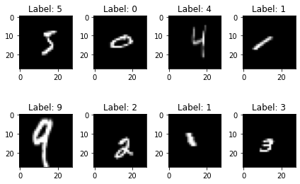
Figure 1: Augmented MNIST data, where each image is randomly shifted, shrunken/stretched and darkened/lightened

A $d\times d$ image is written as bivariate function $f:\mathbb{R}^{2}\rightarrow[0,\infty)$ such that the pixel-wise grayscale values are $f(j/d,\ell/d),$ with $j,\ell=1,\ldots,d.$ Here smaller function values correspond to darker pixels. Alternatively, one could also model the pixel values by the mean intensity over a small square. Since we are interested in larger values for $d,$ there is hardly any difference between both approaches regarding the statistical analysis.

We briefly describe how simple transformations of the image change the function $f.$ Higher function values lighten the grayscale image. Thus, multiplying all pixel values by some factor $\eta>1$ results in a lighter version of the image. Similarly, multiplication of the pixel values with $\eta<1$ leads to a darker version. Moving the object to the right/left or up/down in the image corresponds to a shift of the object on the image by a vector $(\tau,\tau^{\prime}).$ This changes the function $f$ to $(x,y)\mapsto f(x-\tau,y-\tau^{\prime}).$ If the object is stretched out or shrunken in $x$- or $y$-direction, the recorded pixel values will be of the form $f(\xi j/d,\xi^{\prime}\ell/d),j,\ell=\{1,\ldots,d\}$, where $|\xi|<1$ increases the length and $|\xi^{\prime}|<1$ increases the height of the object on the image. Factors $|\xi|,|\xi^{\prime}|>1$ shrink the size of the object. A negative $\xi$ or $\xi^{\prime}$ flips the object in $x$- or $y$-direction. Including lightening/darkening, shifts and scaling, the function $f$ becomes $(x,y)\mapsto\eta f(\xi x-\tau,\xi^{\prime}y-\tau^{\prime}).$

The basic underlying idea of the data generating model is to assume that the two classes correspond to two unknown template functions $f_{0}$ and $f_{1}$ and that every observed image in the dataset is a random transformation of the two classes, where the parameters $(\eta,\tau,\tau^{\prime},\xi,\xi^{\prime})$ are randomly generated from some distribution.

This means that we observe $n$ independently generated pairs of a $d\times d$ image with corresponding class label. The pairs are denoted by $(\mathbf{X}_{i},k_{i})\in[0,\infty)^{d\times d}\times\{0,1\}.$ Each image is represented by a $d\times d$ matrix $\mathbf{X}_{i}=(X^{(i)}_{j,\ell})_{j,\ell=1,\ldots,d}$ with entries

$$X^{(i)}_{j,\ell}=\eta_{i}f_{k_{i}}\Big{(}\xi_{i}\frac{j}{d}-\tau_{i},\xi^{\prime}_{i}\frac{\ell}{d}-\tau^{\prime}_{i}\Big{)},$$ (1)

where $f_{0},f_{1}$ are two unknown functions and $\eta_{i},\xi_{i},\xi_{i}^{\prime},\tau_{i},\tau_{i}^{\prime}$ are unobserved independent random variables. The lightening/darkening factor $\eta_{i}$ is moreover assumed to be positive. Notice that the number of pixels in each image is $d^{2}.$ Throughout the article, we assume that the template functions $f_{0},f_{1}$ are non-negative. Since also $\eta_{i}>0,$ this means that also all pixel values $X^{(i)}_{j,\ell}$ are non-negative.

The support of a function $g$ is the set of all arguments for which the function value is non-zero. For the template functions $f_{0},f_{1},$ we call the function restricted to its support the object. The complement of the support (arguments with function value zero) is called background.

In summary, model (1) generates images of the two objects with template functions $f_{0},f_{1}$ where the shifts $\tau$, $\tau^{\prime}$, scaling $\xi$, $\xi^{\prime}$ and brightness $\eta$ are random.

3 Classification via image alignment

To remove the dependence on the random shift and the random scaling in a given image, one possibility is to rescale it such that the displayed object is on $[0,1]^{2}.$ This approach is similar to curve registration in functional data analysis, see for instance [20]. For a generic image $\mathbf{X}=(X_{j,\ell})_{j,\ell=1,\ldots,d}$ with

$$X_{j,\ell}=\eta f\Big{(}\xi\frac{j}{d}-\tau,\xi^{\prime}\frac{\ell}{d}-\tau^{\prime}\Big{)},$$ (2)

we now describe a transformation $T$ that is nearly invariant under changes of the parameters $\eta,\xi,\xi^{\prime},\tau,\tau^{\prime}.$ This transformation is later applied to the images in the dataset.

We work under the assumption that the object is always completely visible on the image. In mathematical notation, this means that $(x_{1},x_{2})\mapsto f(\xi x_{1}-\tau,\xi^{\prime}x_{2}-\tau^{\prime})$ has support contained in $[0,1]^{2}.$ To achieve this we impose the following constraints.

Assumption 1.

Suppose that $f$ has support contained in $[1/4,3/4]^{2}$, that $\xi,\xi^{\prime}\geq 1/2,$ $3/4-\xi\leq\tau\leq 1/4,$ $3/4-\xi^{\prime}\leq\tau^{\prime}\leq 1/4$ and that $f$ is Lipschitz continuous in the sense that

$$|f(x,y)-f(x^{\prime},y^{\prime})|\leq C_{L}\|f\|_{1}\big{(}|x-x^{\prime}|+|y-y^{\prime}|\big{)}$$ (3)

for some constant $C_{L}$. If $u\in[0,1],$ the assumption implies $\xi u+\tau\in[\tau,\xi+\tau]\subseteq[1/4,3/4]$ and therefore the function $(u,v)\mapsto f(\xi u+\tau,\xi^{\prime}v+\tau^{\prime})$ has support on $[0,1]^{2}.$

For instance if $\xi=\xi^{\prime}=2,$ then $\tau,\tau^{\prime}\in[-5/4,1/4].$ The range of possible shifts $\tau,\tau^{\prime}$ increases as $\xi,\xi^{\prime}$ gets larger. This is reasonable, as larger $\xi,\xi^{\prime}$ mean that the object is shrinked and thus becomes smaller, so that larger shifts, i.e., larger $\tau,\tau^{\prime}$ are possible without pushing the object out of the image.

In a first step, we try to access from the image $\mathbf{X}$ the support of the underlying function $f,$ by finding the smallest axes-aligned rectangle containing all non-zero pixel values. For convenience, we call this the rectangular support. To determine the rectangular support, we denote the smallest and largest occurring indices over all non-zero pixels in the image by

$$j_{-}:=\operatorname*{arg\,min}\big{\{}j:X_{j,\ell}>0\big{\}},\quad j_{+}:=\operatorname*{arg\,max}\big{\{}j:X_{j,\ell}>0\big{\}}$$ (4)

and

$$\ell_{-}:=\operatorname*{arg\,min}\big{\{}\ell:X_{j,\ell}>0\big{\}},\quad\ell_{+}:=\operatorname*{arg\,max}\big{\{}\ell:X_{j,\ell}>0\big{\}}.$$ (5)

Figure 2: Measuring the rectangular support.

The rectangular support of the image is then given by the rectangle $[j_{-}/d,j_{+}/d]\times[\ell_{-}/d,\ell_{+}/d].$ Similarly, we define the rectangular support of a function as the smallest rectangle containing the support. If $f$ has true rectangular support $[\alpha_{-},\alpha_{+}]\times[\beta_{-},\beta_{+}],$ the rectangular support of the rescaled function $(x,y)\mapsto\eta f(\xi x-\tau,\xi^{\prime}y-\tau^{\prime})$ is $R:=[(\alpha_{-}+\tau)/\xi,(\alpha_{+}+\tau)/\xi]\times[(\beta_{-}+\tau^{\prime})/{\xi^{\prime}},(\beta_{+}+\tau^{\prime})/{\xi^{\prime}}].$ From the definition of the model it is now clear that the rectangular support of the image $[j_{-}/d,j_{+}/d]\times[\ell_{-}/d,\ell_{+}/d]$ should be close to $R$ and that these two rectangles are in general not the same, see Figure 2 for an illustration.

The line $[0,1]\ni t\mapsto j_{-}+t(j_{+}-j_{-})$ starts at $j_{-}$ and ends for $t=1$ at $j_{+}.$ Define

$$Z(t,t^{\prime})=X_{\lfloor j_{-}+t(j_{+}-j_{-})\rfloor,\lfloor\ell_{-}+t^{\prime}(\ell_{+}-\ell_{-})\rfloor},$$ (6)

where $\lfloor\cdot\rfloor$ denotes the floor function. The function $(t,t^{\prime})\mapsto Z(t,t^{\prime})$ runs therefore through the pixel values on the rectangular support, rescaled to the unit square $[0,1]^{2}.$ Thus, up to smaller order effects, $Z(t,t^{\prime})$ should not depend anymore on the influence of the random scaling and random shifts in the image.

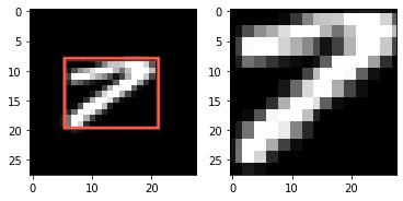
Figure 3: $\mathbf{X}$ vs. $T_{\mathbf{X}}$

To find a quantity that is also nearly independent of the lightening/darkening factor $\eta,$ we apply normalization and consider $Z/\|Z\|_{2}.$ We now define the image alignment transformation

$$T_{\mathbf{X}}=\frac{Z}{|Z|_{2}}.$$ (7)

In the notation $T_{\mathbf{X}}$ we highlight the dependence on $\mathbf{X}$ as this allows us to define the classifier in a concise way. Figure 3 shows the image before and after the transformation $T_{\mathbf{X}}$ is applied. It becomes clear, that the transformation nearly eliminates the influence of random stretching/shrinking and random dilation in the image.

We study the classifier $\widehat{k}$ that uses the label of the $T_{\mathbf{X}_{i}}$ in the dataset closest to $T_{\mathbf{X}}$, that is,

$$\widehat{k}:=k_{\hat{i}},\quad\text{with}\ \ \widehat{i}\in\operatorname*{arg\,min}_{i=1,\dots,n}\,\big{\|}T_{\mathbf{X}}-T_{\mathbf{X}_{i}}\big{\|}_{2}.$$ (8)

Interestingly, this is an interpolating classifier, in the sense that if the new $\mathbf{X}$ coincides with one of the images in the database $\mathbf{X}_{i},$ then, $T_{\mathbf{X}}=T_{\mathbf{X}_{i}}$, $\widehat{i}=i$ and $\widehat{k}=k_{i}.$

If the support of the function $f$ in (2) is a highly unstructured set, it might well happen that the rectangular support of the data as displayed in Figure 2 and the rectangular support of the underlying function $f$ are far apart. This means that the transformation $T$ can still heavily depend on the rescaling variables of the image resulting in possible misclassification of the image. To cope with this, we now introduce a notion of regularity on sets and will later assume that the support of the template functions $f_{k}$ satisfies this condition. Recall that $|\cdot|_{2}$ denotes the Euclidean norm.

Definition 3.1.

Let $\mathcal{C}\subset[0,1]^{2}$ be a closed and connected set with boundary described by a parametrized curve $\phi:[0,1]\rightarrow\mathbb{R}^{2}$ with $\phi(0)=\phi(1)$. For $\Gamma\geq 1$, we say that $\mathcal{C}$ is a $\Gamma$-set if for all $0\leq u\leq v\leq w\leq 1$ and all $t\in[0,u]\cup[w,1],$

$$\Big{(}\big{|}\phi(u)-\phi(v)\big{|}_{2}+\big{|}\phi(v)-\phi(w)\big{|}_{2}\Big{)}\wedge\Big{(}\big{|}\phi(u)-\phi(t)\big{|}_{2}+\big{|}\phi(t)-\phi(w)\big{|}_{2}\Big{)}\leq\Gamma\big{|}\phi(w)-\phi(u)\big{|}_{2}.$$ (9)

The condition can be viewed as a reverted triangle inequality. To understand the inequality in more detail, observe that the two boundary points $\phi(w),\phi(u)$ are connected by the two arcs $\mathcal{A}_{1}=\{\phi(t):t\in[0,u]\cup[w,1]\}$ and $\mathcal{A}_{2}=\{\phi(v):v\in[u,w]\}.$ The condition says that one of these two arcs has the property that for any of the points on it, the sum of the distances to $\phi(u)$ and $\phi(w)$ is at most $\Gamma$ times the distance between $\phi(u)$ and $\phi(w).$ Differently speaking, it means that if we start at $\phi(u)$ and instead of going directly to $\phi(w),$ we first visit a point on the selected arc, the overall distance due to the detour is not more than $\Gamma$ times the direct distance between $\phi(u)$ and $\phi(w)$.

The selected arc is typically the smaller arc. Suppose that $\mathcal{C}$ is a disc and thus, the boundary is a circle. If $u$ and $w$ are taken closer and closer, the right hand side of the inequality in Definition 3.1 will decrease to zero and the condition can only hold for the arc $\mathcal{A}_{2}.$

As regularity condition on $f,$ we will assume that the support of $f$ is a $\Gamma$-set. The next result shows how the deformation of the function $f$ changes the constant $\Gamma.$ In particular, if both directions are stretched or shortened by the same factor, that is, $\xi=\xi^{\prime},$ the support is still a $\Gamma$-set. If we stretch the $x$- and $y$-axis by a different factor, the support can become more deformed resulting in a larger constant in (9).

Lemma 3.2.

If the support of $f$ is a $\Gamma$-set and Assumption 1 holds, then the support of $(x,y)\mapsto\eta f(\xi x-\tau,\xi^{\prime}y-\tau^{\prime})$ is a $(\xi\vee\xi^{\prime})\Gamma/(\xi\wedge\xi^{\prime})$-set.

Example 3.3.

Every disk $\mathcal{C}$ is a $\sqrt{2}$-set.

A proof is provided in Appendix A. Unless the set has a singular point in the sense that $\phi(u)=\phi(w)$ for $u\neq w,$ all ’reasonable’ sets are $\Gamma$-sets, but the constant $\Gamma$ might be large. This is important later, since this will require a larger dimension $d$ to achieve perfect separation of the classes.

Lemma A.1 in the Appendix shows that if the support of $f$ is a $\Gamma$-set, the distance between the two rectangles in Figure 2 is order $\Gamma/d.$

We now state the main result of this section. For that, we first introduce the separation quantity

$$D:=D(f_{0},f_{1})\vee D(f_{1},f_{0}),\quad\text{with}\quad D(f,g):=\frac{\inf_{a,b,b^{\prime},c,c^{\prime}\in\mathbb{R}}\|af(b\cdot+c,b^{\prime}\cdot+c^{\prime})-g\|_{2}}{\|g\|_{2}}.$$ (10)

The result requires the minimal separation condition $D>4K(C_{L}^{2}\vee C_{L})\Xi_{n}^{4}\Gamma^{2}/d.$ This means the template functions $f_{0}$ and $f_{1}$ are separated by $\gtrsim 1/d$ in $L^{2}$-norm uniformly over all possible image deformations.

Theorem 3.4.

Let $(\mathbf{X},k),(\mathbf{X}_{1},k_{1}),\dots,(\mathbf{X}_{n},k_{n})$ be defined as in (1). Suppose that the labels $0$ and $1$ occur at least once in the training data, that is, $\{i:k_{i}=0\}\neq\varnothing$ and $\{i:k_{i}=1\}\neq\varnothing$. Assume moreover that the supports of $f_{0},f_{1}$ are $\Gamma$-sets for some $\Gamma\geq 1$ and that $f_{0}$ and $f_{1}$ satisfy Assumption 1 with Lipschitz constant in (3) bounded by $C_{L}.$ Set $\Xi_{n}:=\max\{\xi,\xi^{\prime},\xi_{1},\xi^{\prime}_{1},\ldots,\xi_{n},\xi^{\prime}_{n}\}$ and let $[\alpha_{-,k},\alpha_{+,k}]\times[\beta_{-,k},\beta_{+,k}]$ be the rectangular support of the function $f_{k}$ in (1) satisfying $(\alpha_{+,k}-\alpha_{-,k})\wedge(\beta_{+,k}-\beta_{-,k})>2\Xi_{n}^{2}(\Gamma+2)/d.$ If $K$ is the universal constant in Lemma A.2, and $D>4K(C_{L}^{2}\vee C_{L})\Xi_{n}^{4}\Gamma^{2}/d$ with $D$ as in (10), then, the classifier $\widehat{k}$ as defined in (8) will recover the correct label, that is,

$$\widehat{k}=k.$$

We also prove a corresponding lower bound. It says that under suitable assumptions, we can find two functions $f_{0}$ and $f_{1},$ separated in the sense that $\|\eta f_{0}\big{(}\xi\cdot+\tau,\xi^{\prime}\cdot+\tau^{\prime}\big{)}-f_{1}\|_{L^{2}(\mathbb{R}^{2})}\gtrsim 1/d,$ and generating the same data. This means that it is impossible to decide from which class the data come from, proving that a $1/d$-separation in $L^{2}$ is necessary to discriminate between the classes.

Theorem 3.5.

Let $d$ be an integer multiple of $4.$ For any $(\eta,\xi,\xi^{\prime},\tau,\tau^{\prime})$ satisfying $\eta>0,\xi,\xi^{\prime}>1/2,\tau<1/4<\tau+\xi/2<3/4<\tau+\xi,\tau^{\prime}<1/4<\tau^{\prime}+\xi^{\prime}/2<3/4<\tau^{\prime}+\xi^{\prime},$ there exist non-negative Lipschitz continuous functions $f_{0},f_{1}$ with $C_{L}=C_{L}(\eta,\xi,\xi^{\prime},\tau,\tau^{\prime}),$ support in $[1/4,3/4]^{2},$ and

$$\big{\|}\eta f_{0}\big{(}\xi\cdot+\tau,\xi^{\prime}\cdot+\tau^{\prime}\big{)}-f_{1}\big{\|}_{L^{2}(\mathbb{R}^{2})}\geq\frac{1}{8d},$$

such that the data generating model (2) can be written as

$$X_{j,\ell}=f_{1}\Big{(}\frac{j}{d},\frac{\ell}{d}\Big{)}=\eta f_{0}\Big{(}\xi\frac{j}{d}+\tau,\xi^{\prime}\frac{\ell}{d}+\tau^{\prime}\Big{)}.$$

Consequently, for different choices of the random deformation parameters, the same data are generated under both classes.

The assumption that $d$ is divisible by $4$ is imposed for technical reasons. Also in practice, $d$ is often a power of $2.$ The proof of the lower bound shows that the rate $1/d$ is due to the Lipschitz continuity of $f_{0},f_{1}.$ Imposing instead Hölder regularity with index $\beta\leq 1,$ it is expected that the lower bound would then be of the order $O(d^{-\beta}),$ which we also conjecture to be the optimal separation rate in this case.

Below we discuss several extensions of the considered framework. To allow objects to be flipped in $x$- and/or $y$-direction, that is, negative $\xi,\xi^{\prime}$ in model (1), a natural generalization of the image alignment classifier is to look for the best fit among all four possibilities for flip/no flip of the $x$- and $y$-axis. This means that if $Z$ is as in (6) and $Z_{1}:=Z,$ $Z_{2}(t,t^{\prime}):=Z(1-t,t^{\prime}),$ $Z_{3}(t,t^{\prime}):=Z(t,1-t^{\prime}),$ $Z_{4}(t,t^{\prime}):=Z(1-t,1-t^{\prime})$, and $T_{\mathbf{X}}^{(r)}:=Z_{r}/\|Z\|_{2},$ for $r=1,2,3,4,$ the modified image alignment classifier $\widehat{k}$ is taken to be

$$\widehat{k}:=k_{\hat{i}},\quad\text{with}\quad\widehat{i}\in\operatorname*{arg\,min}_{i=1,\dots,n}\,\min_{r=1,2,3,4}\big{\|}T_{\mathbf{X}}^{(r)}-T_{\mathbf{X}_{i}}\big{\|}_{2}.$$ (11)

In the presence of background noise, finding the rectangular support of the object is hard and a natural alternative would be to rely on level sets instead. For a function $g$, the $t$-level set is defined by $\{\mathbb{x}:g(\mathbb{x})>t\}$. We then say that the rectangular $t$-level set is the smallest rectangular containing the $t$-level set. For non-negative $g$, the (rectangular) $0$-level set is the (rectangular) support. We can now follow a similar strategy by determining in a first step the $t$-rectangular support of all images in the dataset. Since for $t>0$ the outcomes will depend on the lightening/darkening parameter $\eta$ in model (1), we first need to normalize the pixel values $\mathbb{\overline{X}}_{i}=(\overline{X}_{j,\ell}^{(i)})_{j,\ell=1,\dots,d}$ with $\overline{X}_{j,\ell}^{(i)}:=X_{j,\ell}^{(i)}/|\mathbb{\overline{X}}_{i}|_{2}$ and work with $\mathbb{\overline{X}}_{i}$ instead of $\mathbb{{X}}_{i}.$ The classifier is robust to the background noise, if $t$ exceeds the noise level. Picking a very large $t$ is, however, undesirable as it leads to a small rectangular $t$-level set causing larger constants in the separation condition between the two classes.

If multiple non-overlapping objects are displayed in one image, we suggest to use in a first step an image segmentation method (see, e.g., [11, 21]) and then apply the image alignment classifier to each of the segments.

The image alignment step in the construction of the classifier leads to a representation of the image that is (up to discretization effects) independent of the rescaling and the shift of the object. While image alignment occurs naturally and is mathematically tractable, one could, in principle, also use other methods for this step. For instance, the modulus of the Fourier transform is independent of shifts.

4 Classification with convolutional neural networks

Convolutional neural networks (CNNs) have achieved remarkable practical success in recent years, especially in the context of image recognition [18, 17, 27, 26]. In this section we sketch how one can solve the image classification task with CNNs. Recall that the image alignment classifier introduced in the previous section is up to remainder terms invariant under different scales $\xi,\xi^{\prime}$, translations $\tau,\tau^{\prime}$ and brightness factor $\eta$ of the image. Except for translations, it is not obvious how well these invariances can be learned by a CNN. To address this problem, we first introduce suitable mathematical notation to describe the structure of a CNN. For a general introduction to CNNs see [33, 26].

4.1 Convolutional neural networks

In this work we study CNNs with rectifier linear unit (ReLU) activation function and softmax output layer. Roughly speaking, a CNN consists of three components: Convolutional, pooling and fully connected layers. The input of a CNN is a $d\times d$ matrix containing the pixel values of an image. The convolutional layer uses so-called filters that perform convolution operations on a window of values of the previous layer. Equivalently, a filter can be represented as weight matrix of a pre-defined size that moves across the image. Finally an element-wise nonlinear activation function $\sigma:\mathbb{R}\rightarrow\mathbb{R}$ is applied on the outcome of the convolutions. All values obtained in this way form a so-called feature map.

In this work, we consider CNNs with one convolutional layer followed by one pooling layer. For mathematical simplicity, we introduce a compact notation tailored to this specific setting and refer to [14, 15] for a general mathematical definition. Recall that the input of the network is given by an input image represented by a $d\times d$ matrix $\mathbf{X}$. For a $d\times d$ matrix $\mathbb{W}$, we define its quadratic support $[\mathbb{W}]$ as the smallest quadratic sub-matrix $\mathbb{W}$ such that all entries are zero that are in $\mathbb{W}$ but not in $[\mathbb{W}]$. For example,

$$[\mathbb{W}]=\begin{pmatrix}1&1\\ 0&0\end{pmatrix}.$$

is the quadratic support of the matrix

$$\mathbb{W}=\begin{pmatrix}0&1&1\\ 0&0&0\\ 0&0&0\end{pmatrix}.$$

In our setting $[\mathbb{W}]$ denotes the network filter. To describe the action of the filter on the image $[\mathbb{W}]\star\mathbf{X}$, assume that $[\mathbb{W}]$ is a filter of size $\ell\in\{1,\dots,d\}$. Writing $0_{j\times k}$ for the $j\times k$ zero matrix, we enlarge the matrix $\mathbf{X}$ by appending zero matrices on each side considering

$$\mathbf{X}^{\prime}:=\begin{bmatrix}0_{\ell\times\ell}&0_{\ell\times d}&0_{\ell\times\ell}\\ 0_{d\times\ell}&\mathbf{X}&0_{d\times\ell}\\ 0_{\ell\times\ell}&0_{\ell\times d}&0_{\ell\times\ell}\end{bmatrix}.$$

Let $\mathbf{X}^{\prime}_{i,j}$ be a $\ell\times\ell$ block matrix of $\mathbf{X}^{\prime}$ with entries $(X^{\prime}_{i+a,j+b})_{a,b=0,\dots,\ell-1}.$ In machine learning parlance, this is a patch. Further denote by $([\mathbb{W}]\star\mathbf{X})_{i,j}$ the entrywise sum of the Hadamard product of $[\mathbb{W}]$ and $\mathbf{X}^{\prime}_{i,j}$. The matrix $[\mathbb{W}]\star\mathbf{X}$ contains then all entrywise sums of the Hadamard product of $[\mathbb{W}]$ for all possible choices of $\ell\times\ell$ matrices of $\mathbf{X}^{\prime}$. Finally the ReLU activation function $\sigma(x)=\max\{x,0\}$ is applied elementwise. A feature map can then be described by

$$\sigma([\mathbb{W}]\star\mathbf{X}).$$

The extension of the matrix $\mathbf{X}$ to $\mathbf{X}^{\prime}$ is a form of zero padding and ensures the same in-plane dimension after performing convolution [12]. The pooling layer is typically applied to the feature map. Special kinds of pooling are max- or average pooling. While max-pooling extracts the maximum value from all patches of the feature map, average-pooling takes the average over each patch of the feature map. In this work we consider CNNs with global max-pooling in the sense that the max-pooling extracts from every feature map $\sigma([\mathbb{W}]\star\mathbf{X})$ the largest absolute value. Since each convolutional layer is usually followed by a pooling layer, we say that the CNN has one hidden layer, if one convolutional and one pooling layer are applied consecutively. The feature map after global max-pooling is then given by the value

$$\mathbb{O}=|\sigma([\mathbb{W}]\star\mathbf{X})|_{\infty}.$$

For $k$ filters described by the matrices $\mathbb{W}_{1},\ldots,\mathbb{W}_{k},$ we obtain then the $k$ values

$$\mathbb{O}_{s}=|\sigma([\mathbb{W}_{s}]\star\mathbf{X})|_{\infty},\quad s=1,\ldots,k.$$ (12)

We denote by $\mathcal{F}^{C}(1,k)$ the class of CNNs with one hidden layer and $k$ feature maps of the form (12). The output of these networks is typically flattend, i.e., transformed into a vector, before several fully connected layers are applied. The ReLU activation function is again the common choice for these layers. For any vector $\mathbb{v}=(v_{1},\dots,v_{r})^{T}$, $\mathbb{y}=(y_{1},\dots,y_{r})^{T}\in\mathbb{R}^{r}$, we define $\sigma_{\mathbb{v}}\mathbb{y}=(\sigma(y_{1}-v_{1}),\dots,\sigma(y_{r}-v_{r}))^{T}$. As we consider a binary classification task, the last layer of the network should extract a two-dimensional probability vector. To do this, it is standard to apply the softmax function

$$\Phi_{\beta}(x_{1},x_{2})=\left(\frac{e^{\beta x_{1}}}{e^{\beta x_{1}}+e^{\beta x_{2}}},\frac{e^{\beta x_{2}}}{e^{\beta x_{1}}+e^{\beta x_{2}}}\right).$$ (13)

Here $\beta>0$ is a pre-chosen parameter. A network with $L\in\mathbb{N}$ fully connected hidden layers and width vector $\mathbb{m}=(m_{0},\dots,m_{L+1})\in\mathbb{N}^{L+2}$, where $m_{i}$ denotes the number of hidden neurons in the $i$-th hidden layer, can then be described by a function $f:\mathbb{R}^{m_{0}}\rightarrow\mathbb{R}^{m_{L+1}}$ with

$$\mathbb{x}\mapsto f(\mathbb{x})=\psi\mathbb{W}_{L}\sigma_{\mathbb{v}_{L}}\mathbb{W}_{L-1}\sigma_{\mathbb{v}_{L-1}}\cdots\mathbb{W}_{1}\sigma_{\mathbb{v}_{1}}\mathbb{W}_{0}\mathbb{x},$$

where $\mathbb{W}_{j}$ is a $m_{j}\times m_{j+1}$ weight matrix, $\mathbb{v}_{j}$ is the $j$-th shift vector and $\psi$ is either the identity function $\psi=id$ or the softmax function $\psi=\Phi_{\beta}.$ We denote this network class of fully connected neural networks by $\mathcal{F}_{\psi}(L,\mathbb{m})$.

For the CNN we work with a specific architecture by considering the class

$$\begin{split}\mathcal{G}_{\psi}(m)=\Big{\{}f\circ g:&f\in\mathcal{F}_{\psi}\big{(}1+2\lceil\log_{2}m\rceil,(2m,4m,\ldots,4m,2)\big{)},g\in\mathcal{F}^{C}(1,2m)\Big{\}}\end{split}$$ (14)

for a positive integer $m.$ As we consider only one convolutional/pooling layer, the number of feature maps equals the input dimension of the fully connected subnetwork.

By construction, CNNs can capture invariance under shifts in the input. This means that up to boundary and discretization effects, the CNN classifier does not depend on the values of the dilation parameters $\tau$ and $\tau^{\prime}$ in (2). The underlying reason is that the filters are applied to all patches. A shift of the image pixels causes therefore a permutation of the values in the feature map. For example, if a cat on an image is shifted from the upper left corner to the lower right corner, the convolutional filter will generate, up to discretization effects, the same feature values at possibly different locations in the feature map. Since the global max-pooling layer is invariant to permutations, the CNN output is thus invariant under translations.

More challenging for CNNs are different object sizes. In our image deformation model they are represented through different scale factors $\xi,\xi^{\prime}.$ An interesting question is whether it is desirable to construct a scale-invariant CNN at all. [32, 25, 7] emphasize the importance of scale-variance for the performance of a CNN. The reason is that different scales often come with different resolutions of the image. For instance, low resolution images consist of fewer pixels, meaning that small objects with fine scale cannot be detected on them. But even if a small object is still recognisable, it remains hard to detect it. [7] highlights that forcing a filter to be scale-invariant means that we miss image structure, which is relevant for the task. According to this reasoning, object recognition even benefits from scale-variant information. Motivated by these findings, the main result presents a CNN architecture, which is able to classify objects of different sizes by using for each possible scale factor a suitable convolutional filter.

4.2 A misclassification bound for CNNs

We first provide an extension of Assumption 1 that also allows flipping of the image, that is, negative value for $\xi,\xi^{\prime}.$

Assumption 1’.

Suppose that $f$ has support contained in $[1/4,3/4]^{2}$, that $|\xi|,|\xi^{\prime}|\geq 1/2,$ $3/4-(\xi)_{+}\leq\tau\leq 1/4+(-\xi)_{+},$ $3/4-(\xi^{\prime})_{+}\leq\tau^{\prime}\leq 1/4+(-\xi^{\prime})_{+}$ and that $f$ is Lipschitz continuous in the sense that

$$|f(x,y)-f(x^{\prime},y^{\prime})|\leq C_{L}\|f\|_{1}\big{(}|x-x^{\prime}|+|y-y^{\prime}|\big{)}$$ (15)

for some constant $C_{L}$.

Similarly as in Assumption 1, it can be checked that the function $(u,v)\mapsto f(\xi u+\tau,\xi^{\prime}v+\tau^{\prime})$ has support on $[0,1]^{2}.$

We suppose that the training data consist of $n$ i.i.d. data, generated as follows. For $\pi\in[0,1]$ and each $i,$ we draw a label $k_{i}\in\{0,1\}$ from the Bernoulli distribution with success probability $\pi.$ Let $Q$ be a distribution on the parameters $\eta,\xi,\xi^{\prime},\tau,\tau^{\prime}$ that is supported on parameter values satisfying Assumption 1’. The $i$-th sample is then $(\mathbf{X}_{i},k_{i}),$ where $\mathbf{X}_{i}$ is an independent draw from model (1) with template function $f_{k_{i}}$, parameters $(\eta_{i},\xi_{i},\xi_{i}^{\prime},\tau_{i},\tau_{i}^{\prime})$ generated from $Q$ and corresponding label $k_{i}.$ The full dataset is then

$$\mathcal{D}_{n}=\big{(}(\mathbf{X}_{1},k_{1}),\dots,(\mathbf{X}_{n},k_{n})\big{)}.$$ (16)

In expectation it consists of $n(1-\pi)$ samples from class $0$ and $n\pi$ samples from class $1.$

We now describe how the CNN parameters are fitted given the data. As a pre-processing step, the pixel values are normalized

$$\overline{\mathbb{X}}_{i}=(\overline{X}_{j,\ell}^{(i)})_{j,\ell=1,\dots,d},\quad\ \text{with}\ \ \overline{X}_{j,\ell}^{(i)}:=\frac{X_{j,\ell}^{(i)}}{\sqrt{\sum_{j,k=1}^{d}(X_{j,\ell}^{(i)})^{2}}}.$$

The normalized images are invariant under different values of $\eta$ and all pixel values lie between $0$ and $1$.

For binary classification, the neural network has two outputs and the corresponding output vector $\mathbf{Y}_{i}=(1-k_{i},k_{i})$ decodes the class label as one of the two-dimensional standard basis vectors. It is $\mathbf{Y}_{i}=(1,0)$ if $k_{i}=0$ and $\mathbf{Y}_{i}=(0,1)$ for $k_{i}=1.$

Fitting a neural network with softmax output to the dataset results in estimators for the conditional class probabilities (or aposteriori probabilities).

In this article we consider fitting a CNN of the form (14) via least squares

$$\widehat{\mathbb{p}}\in\ \operatorname*{arg\,min}_{\mathbb{p}\in\mathcal{G}_{\Phi_{\beta}}(m)}\frac{1}{2n}\sum_{i=1}^{n}\big{|}\mathbf{Y}_{i}-\mathbb{p}(\overline{\mathbf{X}}_{i})\big{|}_{2}^{2}=\operatorname*{arg\,min}_{\mathbb{p}=(p_{1},p_{2})\in\mathcal{G}_{\Phi_{\beta}}(m)}\frac{1}{n}\sum_{i=1}^{n}\big{(}k_{i}-p_{2}(\overline{\mathbb{X}}_{i})\big{)}^{2}.$$ (17)

To see the equality, observe that $(p_{1},p_{2})$ denote the two outputs of the CNN. Since $\mathbf{Y}_{i}=(1-k_{i},k_{i}),$ we have $|\mathbf{Y}_{i}-\mathbb{p}(\mathbf{X}_{i})|_{2}^{2}=2(k_{i}-p_{2}(\mathbb{X}_{i}))^{2}.$

We choose the least squares functional here as we can rely on existing oracle inequalities. From an applied point of view, the cross-entropy would be more appealing, see, e.g., [8, 16, 30, 2]. As common in the statistical theory for deep learning, we choose the global risk minimizer and do not investigate any specific gradient descent method. Recall that the learned network $\widehat{\mathbb{p}}$ outputs estimands for the two conditional class probabilities $\mathbb{P}(k=0|\mathbf{X})$ and $\mathbb{P}(k=1|\mathbf{X}).$ The standard way to obtain a classifier for the label from this is to take the class with the higher probability, i.e., the classifier $\widehat{k}=1$ if the estimated conditional class probability $\mathbb{P}(k=1|\mathbf{X})$ is larger than zero and $\widehat{k}=0,$ otherwise.

We now state the main result bounding the misclassification error for CNNs. In contrast to the theoretical analysis of the image alignment classifier, we do not need to assume that the support of the functions $f_{0},f_{1}$ is a $\Gamma$-set. Moreover, no network sparsity has to be imposed.

Theorem 4.1.

Consider the classification model (16) with $n>4$. Suppose $f_{0}$ and $f_{1}$ satisfy Assumption 1’ and that $\Xi$ is a positive integer. Let $\widehat{\mathbb{p}}$ be the estimator in (17) for a CNN class $\mathcal{G}_{\Phi_{\beta}}((2\Xi d+1)^{2})$ with $\beta\geq d.$ Suppose a new datapoint $(\mathbf{X},k)$ is independently generated from the same distribution as $(\mathbf{X}_{1},k_{1}).$ If $\widehat{k}$ is the classifier based on $\widehat{\mathbb{p}}$ and the separation constant in (10) satisfies $D^{2}\geq(4\kappa\Xi^{4}+2)/d$, then, there exists a universal constant $\widetilde{C}$ such that

$$\mathbb{P}\big{(}\,\widehat{k}(\mathbf{X})\neq k\,\big{)}\leq\frac{\widetilde{C}\sqrt{\log n}(\Xi d)^{2}\log^{3/2}(3\Xi d)}{\sqrt{n}}\vee e^{-\beta\kappa\Xi^{4}/d}.$$ (18)

Taking for instance $\beta=d^{2}$, $\Xi$ fixed and $n\gtrsim d^{4+q}\log^{4}d$ for some $q>0$, the misclassification error is

$$\mathbb{P}\big{(}\,\widehat{k}(\mathbf{X})\neq k\,\big{)}\lesssim d^{-q}.$$

It can be checked that the number of network parameters in the CNN is of the order $d^{4}\log d.$ Up to logarithmic factors, this means that we obtain a consistent classifier if the sample size is of a larger order than the number of network parameters.

We conjecture that data augmentation can reduce the sample complexity. By assuming that the separation quantity in (10) is positive, our classification model ensures that rescaling of the object size, object shifts and scaling of the pixel intensity do not change the image label. Hence by applying these transformations to the training data, we can generate new labelled images. Potentially this leads also to images with objects outside of the image domain. By determining the rectangular support, we can filter those ones out. The main challenge from a theoretical perspective is that this schemes generates dependency among the training samples. As the learning theory heavily relies on the independence assumption, a completely new theoretical framework is required to derive risk bounds in this setup.

The result implies that the CNN misclassification error can become arbitrary small and this is in line with the nearly perfect classification results of deep learning for a number of image classification tasks. Interestingly most of the previous statistical analysis for neural networks considers settings with non-vanishing prediction error. Those are statistical models where every new image contains randomness that is independent of the training data and can therefore not be predicted by the classifier. To illustrate this, consider the nonparametric regression model $Y_{i}=f(\mathbf{X}_{i})+\sigma\varepsilon_{i},$ $i=1,\ldots,n$ with fixed noise variance $\sigma^{2}$. The squared prediction error of the predictor $\widehat{Y}=\widehat{f}_{n}(\mathbf{X})$ for $Y$ is $E(\widehat{Y}-Y)^{2}=\sigma^{2}+E\big{[}(\widehat{f}_{n}(\mathbf{X})-f(\mathbf{X}))^{2}\big{]}.$ This means that even if we can learn the function $f$ perfectly from the data, the prediction error is still at least $\sigma^{2}.$ Taking a highly suboptimal, but consistent estimator $\widehat{f}_{n}$ for $f$ has prediction error $\sigma^{2}+o(1)$ and thus achieves the lower bound $\sigma^{2}$ up to a vanishing term. This shows that optimal estimation of $f$ only changes the rate of the second order for the prediction error. Because the prediction error cannot vanish and the quality of the estimator $\widehat{f}_{n}$ is of secondary importance, such models are less suitable to explain the success of deep learning. Classification and regression are closely related and the same phenomenon occurs also in classification, whenever the conditional class probabilities lie strictly between $0$ and $1$. Similarly as the argument above, [5] shows that the one nearest neighbor classifier that does not do any smoothing and leads to suboptimal rates for the conditional class probabilities, is optimal for the misclassification error up to a factor $2.$ The only possibility to achieve small misclassification error requires that the conditional class probabilities are always either near zero or one, which is the same as saying that the covariates $X$ carry almost all the information about the label $Y,$ [2]. Our image deformation model has this property, see Lemma 4.3 below.

To prove the theorem, we bound the $L_{2}$ error of the estimator $\widehat{\mathbb{p}}=(\widehat{p}_{1},\widehat{p}_{2})$. By (22), combined with Theorem 1.1 in [10],

$$\mathbf{P}\big{(}\widehat{k}(\mathbf{X})\neq k|\mathcal{D}_{n}\big{)}\leq 2\sqrt{\int_{\mathbb{R}^{d^{2}}}\big{(}\widehat{p}_{2}(\mathbf{x})-p(\mathbf{x})\big{)}^{2}\mathbf{P}_{\mathbf{X}}(d\mathbf{x})}.$$ (19)

with $p(\mathbf{x})=P(k=1|\mathbf{X}=\mathbf{x})$ the conditional class probability. For the right hand side, we can rely on existing oracle inequalities (Lemma B.6) decomposing the $L^{2}$-error into an approximation error and a sample complexity term. The approximation error is controlled using the following bound.

Theorem 4.2.

Suppose $f_{k}$ satisfies Assumption 1’ and that $\Xi$ is a positive integer. There exists a CNN $\widehat{\mathbb{p}}\in\mathcal{G}_{\Phi_{\beta}}((2\Xi d+1)^{2})$ and a constant $\kappa$ only depending on the Lipschitz constants $C_{L_{f_{0}}}$ and $C_{L_{f_{1}}}$ such that if $(\mathbf{X},k)$ is generated in the same way as the data in (16) and $\mathbf{Y}=(1-k,k),$ then

$$|\widehat{\mathbb{p}}(\mathbf{X})-\mathbb{Y}|_{\infty}\leq e^{\beta\big{(}\frac{\kappa\Xi^{4}}{d}-\frac{D^{2}}{2}\big{)}},\ \text{almost surely.}$$

Moreover, if the separation quantity $D$ in (10) satisfies $D>2\Xi^{2}\sqrt{\kappa/d},$ then $|\widehat{\mathbb{p}}(\mathbf{X})-\mathbb{Y}|_{\infty}\leq e^{-\beta(\kappa\Xi^{4})/d},$ almost surely.

If $\beta\gg d,$ the previous result shows then that the approximation error converges to zero if

$$D\gtrsim\frac{1}{\sqrt{d}}.$$ (20)

The key step in the approximation theory is to show that for an input image generated by $f_{k}(\xi\cdot-\tau,\xi^{\prime}\cdot-\tau^{\prime})$ and for any Lipschitz continuous and $L^{2}$-normalized $\phi,$ we can find a filter such that the output of the feature map after applying the global max-pooling layer is

$$\max_{s,t}\frac{\int\phi(u-s,v-t)f_{k}(\xi u-\tau,\xi^{\prime}v-\tau^{\prime})\,dudv}{\|f_{k}(\xi\cdot-\tau,\xi^{\prime}\cdot-\tau^{\prime})\|_{2}}+O\Big{(}\frac{1}{d}\Big{)},$$ (21)

By Cauchy-Schwarz, the largest possible value for the main term is one and it is attained if $\phi(x,y)=f_{k}(\xi x,\xi^{\prime}y)/\|f_{k}(\xi\cdot,\xi^{\prime}\cdot)\|_{2}.$ This motivates to choose as filters all functions of this form. After the global max-pooling layer, we should see then one value of size $1+O(1/d).$ The fully connected layers that are applied afterwards can detect whether this value came from a filter with $k=0$ or $k=1$ and output correspondingly a value that is close to $(1,0)$ if $k$ was $0$ and $(0,1)$ if $k$ was $1.$ There are still a number of complications. The first one is that $\xi$ and $\xi^{\prime}$ are continuous parameters. As it is desirable to have a small number of filters, we only include filters for a discrete grid of $\xi,\xi^{\prime}$ values. This leads to the $O(d^{2})$ many filters and creates additional approximation errors that have to be controlled. Another complication is the $O(1/d)$ remainder term in (21). Due to this term it could happen that if $f_{0}$ and $f_{1}$ are close, the maximum value after the pooling layer is generated from the wrong class which then leads to misclassification. To avoid this, we need in Theorem 4.1 that the separation constant $D$ in (20) satisfies $\gtrsim 1/\sqrt{d},$ where everything except for $d$ is treated here as a constant. This is a stronger requirement than for the object alignment classifier, which only requires $D\gtrsim 1/d,$ see Theorem 3.4. We argue that the $1/d$ lower bound would also work for CNNs but at the cost of a much more involved construction and $O(d^{4})$ filters instead of $O(d^{2})$ filters. To sketch the construction, assume for the moment that the image was generated by $f_{k}\in\{f_{0},f_{1}\}$ with $\eta=\xi=\xi^{\prime}=1$, $\tau=\tau^{\prime}=0,$ and $\|f_{0}\|_{2}=\|f_{1}\|_{2}=1.$ Taking in (21) $\phi(u,v)=(f_{1}(u,v)-f_{0}(u,v))/\|f_{1}-f_{0}\|_{2}$ and ignoring the maximum over $s,t$ by just considering at the moment $s=t=0,$ we find

$$\frac{\int\phi(u,v)f_{k}(u,v)\,dudv}{\|f_{k}\|_{2}}+O\Big{(}\frac{1}{d}\Big{)}=\frac{\int(f_{1}(u,v)-f_{0}(u,v))f_{k}(u,v)\,dudv}{\|f_{1}-f_{0}\|_{2}}+O\Big{(}\frac{1}{d}\Big{)}=\frac{(-1)^{k+1}}{2}\|f_{1}-f_{0}\|_{2}+O\Big{(}\frac{1}{d}\Big{)},$$

indicating that one can discriminate between the two classes if $\|f_{1}-f_{0}\|_{2}\gtrsim 1/d.$ The larger number of filters $O(d^{4})$ in this case is due to the fact that we need to take all filters such that $\phi_{\xi_{0},\xi_{0}^{\prime},\xi_{1},\xi_{1}^{\prime}}(u,v)=(f_{1}(\xi_{1}u,\xi_{1}^{\prime}v)-f_{0}(\xi_{0}u,\xi_{0}^{\prime}v))/\|f_{1}(\xi_{1}\cdot,\xi_{1}^{\prime}\cdot)-f_{0}(\xi_{0}\cdot,\xi_{0}^{\prime}\cdot)\|_{2},$ over a discretized set of values $\xi_{0},\xi_{0}^{\prime},\xi_{1},\xi_{1}^{\prime}.$ The main reason why we have not followed this approach is the envisioned extension to the multiclass case, where images are generated by $K$ template functions $f_{0},\ldots,f_{K}$. While in the proof of Theorem 4.2, the filters depend on one class, the extension described above requires to scan with the filters for all differences $f_{k}-f_{\ell},$ $k\neq\ell,$ which scales of course quadratically in the number of classes $K$.

A consequence of the approximation bound is that under the separation condition in Theorem 4.2, the label can be retrieved from the image.

Lemma 4.3.

Work under the conditions of Theorem 4.2 with $\beta\geq d,$ $D^{2}>(2\kappa\Xi^{4}+2)/d$ and $\kappa$ as in Theorem 4.2. If $(\mathbf{X},k)$ is generated in the same way as the data in (16), then, $k$ can be written as a deterministic function evaluated at $\mathbf{X}$ and we have

$$p(\mathbf{X})=k(\mathbf{X}),$$

with $p(\mathbf{x})=P(k=1|\mathbf{X}=\mathbf{x})$ the conditional class probability.

A consequence is that under the imposed conditions

$$\min_{q:[0,1]^{2}\rightarrow\{0,1\}}\mathbb{P}(q(\mathbf{X})\neq k(\mathbf{X}))=0.$$ (22)

5 Numerical results

This section provides a comparison of the image alignment classifier (8) (abbrv. IAC) and the CNNs on data examples. While the image alignment classifier is implemented following the construction for (8), the CNN architecture for the neural network is slightly modified. In particular, we analyze three different architectures. CNN1 has one convolutional layer with $28$ filters of size $3$, one pooling layer with patch size $2$ and one fully connected layer with $128$ neurons, before applying the softmax layer. CNN2 follows the same architecture as CNN1, but here we apply three convolutional layer with $28$, $64$ and $128$ filters, respectively. CNN3 equals the architecture of CNN2, but consists additionally of three fully connected layers with $128$ neurons, respectively. All CNNs are fitted using the Adam optimizer in Keras (Tensorflow backend) with default learning rate $0.01$. In [29] different settings of CNNs, i.e., with different numbers of convolutional layers, different sizes of filters and different sizes of patches are compared on the MNIST datasets. It is shown that all settings achieve a comparable high validation accuracy. It is therefore sufficient to limit ourselves to the above mentioned three settings.

We generate data based on MNIST [6]. MNIST consists of $60.000$ examples of $28\times 28$ handwritten digits from $0$ to $9.$ In our setting, this means that $d=28.$ As we consider binary classification in this article, we pick two of these classes. Inspired by the random deformation model (1), from each class we choose one or multiple images of handwritten digits and randomly deform them in different ways by applying Keras ImageDataGenerator. The transformed images are randomly shifted (corresponding to $\tau,\tau^{\prime}$ in (1)), randomly shrinked or scaled (corresponding to $\xi,\xi^{\prime}$ in (1)) and randomly lightened or darkened (corresponding to $\eta$ in (1)). Examples of randomly transformed images are shown in Figure 4.

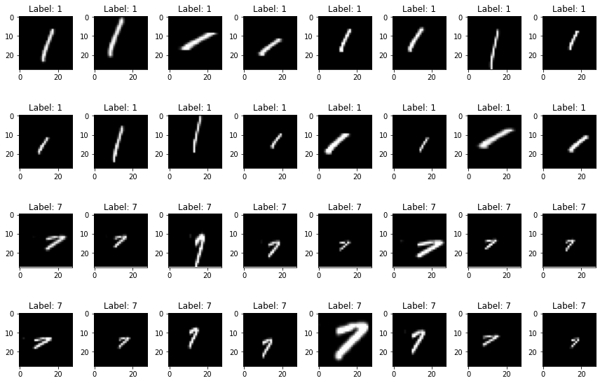
Figure 4: Augmented versions of number 1 (first two rows) and number 7 (last two rows) of the MNIST data set

We consider three different classification task. In the first two tasks we select one sample of each class from MNIST and generate the full dataset by random deformations as described above. In Task 1 we classify the digits $0$ and $4.$ Since these two classes are easy to separate, this task is easy. As a second task, we consider the same setting with the digits $1$ and $7.$ Discrimination between the two classes is slightly harder due to the similarity of the two digits.

For Task 3, we consider a generalization of the image deformation model. In continental Europe the digit $7$ is written 7   with an additional middle line. To incorporate different basic types of the same class, a natural extension of the image deformation model (1) is to assume that every class is describe by random deformation of more than one template functions. In the binary classification case, the template functions are $f_{0,1},\ldots,f_{0,m_{0}}$ for class $0$ and $f_{1,1},\ldots,f_{1,m_{1}}$ for class $1.$ Extending (1), each image is then a $d\times d$ matrix $\mathbf{X}_{i}=(X^{(i)}_{j,\ell})_{j,\ell=1,\ldots,d}$ with entries

$$X^{(i)}_{j,\ell}=\eta_{i}f_{k_{i},r_{i}}\Big{(}\xi_{i}\frac{j}{d}-\tau_{i},\xi^{\prime}_{i}\frac{\ell}{d}-\tau^{\prime}_{i}\Big{)},$$ (23)

for $r_{i}\in\{0,\ldots,m_{k_{i}}\}.$

In Task 3 we sample from this model with $m_{0}=m_{1}=10.$ To this end, we draw ten different images of digits $0$ and ten different images of digits $4$ from MNIST and randomly deform them again by applying Keras ImageDataGenerator. Even in this more general framework, one expects that all classifiers should be able to classify these images properly.

For each of the three tasks all classifiers are trained with $n$ labelled sample images and balanced design, that is, we observe $n/2$ many images from each of the two classes. Our theory suggests that small sample sizes will lead already to negligible (or even vanishing) classification error. We therefore study all methods for sample sizes $n=\{2,4,8,16,32,64\}.$ The quality of each classifier $\widehat{k}$ is measured by the empirical misclassification risk (test error)

$$R_{N}=\frac{1}{N}\sum_{i=1}^{N}\mathbb{1}\big{(}\,\widehat{k}(\mathbb{X}_{n+i})\neq k_{n+i}\big{)},$$

based on the test data $(\mathbf{X}_{n+1},k_{n+1}),\ldots,(\mathbf{X}_{N},k_{N}),$ which are independently generated from the same distribution as the training data. We choose $N=100$ and report the median of the test error over $30$ repetitions for each setting.

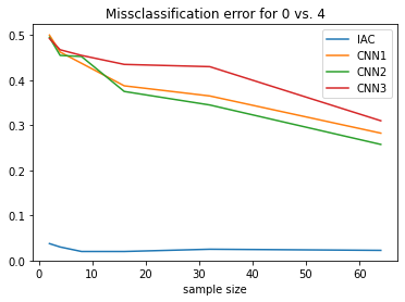
(a) Task 1

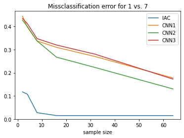
(b) Task 2

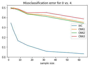
(c) Task 3

Figure 5: Comparison of trained CNN (orange) and image alignment classifier (8) (blue). Reported is the median of the test error over $30$ repetitions for varying size of training sample and the three tasks described in the main text.

In accordance with the theory, the image alignment classifier (8) clearly outperforms the CNN classifiers for all three tasks. Even if we have only $2$ training samples in Task 1, the test error of this classifier is already close to zero. In the second, slightly more difficult, task the test error is $0.12$ for $n=2$ and is close to zero for sample sizes exceeding $16$. The performance of the CNN classifiers improves with increasing training sample, but the misclassification error remains still large. This is of course expected since the CNN needs to learn the invariances due to the random deformations. For Task 3, all classifiers have large misclassification error for small training samples. Recall that in this case the training data are generated based on random deformations from ten different template images of the digits $0$ and $4$. The image alignment classifier will be more likely to misclassify a test image if it is a random deformation of a template image that did not occur in the training set causing the large misclassification error for few training data. Once the image alignment classifier has seen a randomly deformed sample from each of the ten different template images, it is able to classify the test data perfectly. Interestingly, the performance of the CNN classifiers in Task $3$ deteriorates only slightly compared to the previous two tasks. This is due to the fact that image alignment classifier heavily exploits the specific structure of the image deformation model (1), while CNNs are extremely flexible and can adapt to various structures in the data. This flexibility has as a price that large sample sizes are necessary. One should also mention that the image alignment classifier is much simpler to compute. The choice of the CNN architecture has only a minor influence on the performance. While CNN2 is the best classifier for all three tasks, the other two are only slightly worse.

In summary, the empirical results are consistent with the derived theory. The image alignment classifier, that is adapted to the specific structure of the image deformation model (1) has, as expected, much smaller test error if compared to the CNN classifier. In accordance with Theorem 3.4, even for rather small sample sizes, this classifier can classify perfectly. An interesting open question is to combine both methods.

6 General image deformation models

The considered simple image deformation model (1) is based on the assumption that different images of the same object can be generated by simply varying a standard (or template) object in its scale, intensity and position. The view that different images of the same object are created by deforming a template image is consistent with Grenander’s and Mumford’s seminal work on pattern recognition that distinguishes between pure images and deformed images that are generated from pure images by some deformations, see, e.g., [9, 22].

Extensions to background noise and multiple objects have briefly been discussed in Section 3. Another highly relevant extension is the case of partially visible objects. In this scenario it seems unreasonable to base methods on global characteristics of the object such as the support. But it might still be possible to construct classifiers and obtain similar theoretical guarantees by focusing on local properties such that for a correct classification it is sufficient that only some of these local characteristics are completely visible in the image.

In a series of article [19, 3, 4], Mallat and co-authors propose to replace the shifts $\tau$ and $\tau^{\prime}$ by functions. This means that the pixel value at $(x,y)$ in the template image is moved to $(x-\tau(x,y),y-\tau^{\prime}(x,y)).$ These transformations generate a rich class of local deformations. Without any constraints on the functions $\tau,\tau^{\prime},$ however, similar classes are merged, such as the classes corresponding to the digits $1$ and $7$ in handwritten digit classification. To avoid this, [4] imposes a Lipschitz condition on the shifts controlling the amount of local variability. It is moreover shown that a hierarchical wavelet transformation named scattering convolution network is stable to such deformations. In this method, dilated and rotated wavelets are applied in the convolutional layers. All filters are chosen independently of the data and no learning is required. As the focus of the past analysis is on local shifts, it remains unclear to which extend scattering convolution networks can adapt to rescaling of objects.

In [23] and Section 5 in [24], Mumford and Desolneux discuss different deformation classes, including noise and blurr, multi-scale superposition, domain warping and interruptions. To improve our understanding of image classification, one wants to follow a similar program as outlined in this work: Starting with formalizing such deformation classes in a statistical model, then designing optimal methods and analyzing how widely applied procedures such as deep learning perform.

Various sophisticated image deformation models have been proposed in medical image registration. Given a target image $T$ and a source image $S$, image registration aims to find the transformation from $T$ to $S$ that optimizes (in a suitable sense) the alignment between $T$ and $S$. To study and compare image registration methods, it is essential to construct realistic image deformation models describing the generation of the deformed image $T$ from the template $S.$ The survey article [31] classifies these deformation models into several categories, such as ODE/PDE based models, interpolation-based models and knowledge-based models. A simple ODE based random image deformation model is the following: If $\mathbf{X}$ denotes the template/source image, generate a random vector field $u.$ This can be done for instance by taking a basis and generating independent random coefficients according to a fixed distribution. Given $u,$ generate a continuous image deformation $\mathbf{X}(t)$ solving the differential equation $\partial_{t}\mathbf{X}(t)=u(\mathbf{X}(t))$ with $\mathbf{X}(0)=\mathbf{X}.$ The randomly deformed image is then $\mathbf{X}(1)$. DARTEL [1] is a popular image registration method for this deformation model.

The image alignment classifier in Section 3 can be viewed as a combination of image registration and nearest neighbor classifier. Extending this construction to an arbitrary registration method results in the following procedure: Given a new image compute an image alignment with respect to all images in the dataset. As second step, classify the new image by the label of the image in the dataset with the smallest cost for image alignment. Challenges for future research are to provide computationally efficient algorithms and theoretical guarantees.

Another possible generalization of the image deformation model (1) is to think of the two classes as two low-dimensional manifolds $\mathcal{M}_{0},\mathcal{M}_{1}$ in the space of all $d\times d$ grayscale images $[0,\infty)^{d^{2}}.$ This means that an image from class $k\in\{0,1\}$ is a sample from the manifold $\mathcal{M}_{k}.$ In particular, model (1) can be written in this form, where the manifold dimensions are the same as the number of parameters in the model (five).

To summarize, we want to emphasize that for an improved understanding of image classification methods such as CNNs, it is crucial to extend the statistical analysis in this work to more general image deformation models. Various image deformation models have been proposed in the literature. Analyzing them theoretically will help us to build better image classification algorithms. This interplay between data models and algorithms is in line with Grenander’s claim that the analysis of the patterns in a signal and the synthesis of these signals are inseparable problems ([9, 24]).

Appendix A Proofs for Section 3

Proof of Lemma 3.2.

Assumption 1 guarantees that the support of $(x,y)\mapsto\eta f(\xi x-\tau,\xi^{\prime}y-\tau^{\prime})$ is contained in $[0,1]^{2}.$ By assumption, $f$ is a $\Gamma$-set. Let $\phi=(\phi_{1},\phi_{2})^{\top}:[0,1]\rightarrow\mathbb{R}^{2}$ be the parametrized curve describing the boundary of the support of $f.$ The boundary of the support of the function $(x,y)\mapsto\eta f(\xi x-\tau,\xi^{\prime}y-\tau^{\prime})$ can then be described by the parametrized curve

$$s\mapsto\widetilde{\phi}(s):=\Big{(}\frac{\phi_{1}(s)+\tau}{\xi},\frac{\phi_{2}(s)+\tau^{\prime}}{\xi^{\prime}}\Big{)}^{\top}.$$

For any two values $r,s\in[0,1],$ we have $|\phi(r)-\phi(s)|_{2}/(\xi\vee\xi^{\prime})\leq|\widetilde{\phi}(r)-\widetilde{\phi}(s)|_{2}\leq|\phi(r)-\phi(s)|_{2}/(\xi\wedge\xi^{\prime}).$ Using the fact that $\phi$ satisfies (9), we conclude that $\widetilde{\phi}$ satisfies (9) with $\Gamma$ replaced by $(\xi\vee\xi^{\prime})\Gamma/(\xi\wedge\xi^{\prime}).$ This completes the proof. ∎

Proof of Example 3.3. In the following we denote by $\Delta_{ABC}$ the triangle with vertices $A,B$ and $C$ and by $S(\mathbf{x},r)$ the circle with center $\mathbf{x}$ and radius $r$.

Figure 6: Sketch for proof.

Let $\phi(u),\phi(w)$ be two arbitrary points on the boundaries of the disk $\mathcal{C}$ fulfilling $0\leq u\leq w\leq 1$ (see Figure 6). The line $L:=\{\phi(u)+t(\phi(w)-\phi(u)):t\in\mathbb{R}\}$ separates the disk in two parts, such that the circle is splitted in two arcs $\mathcal{A}_{1}=\{\phi(t):t\in[0,u]\cup[w,1]\}$ and $\mathcal{A}_{2}=\{\phi(v):v\in[u,w]\}$. Without loss of generality, we assume in the following that $\mathcal{A}_{1}$ is the smaller arc. We now draw a circle $\mathcal{C}^{\prime}:=S\left(\frac{\phi(u)+\phi(w)}{2},\frac{|\phi(u)-\phi(w)|_{2}}{2}\right)$. For every point $\phi(v)\in\mathcal{A}_{1}$ we then find a point $x^{\prime}\in\mathcal{C}^{\prime}$ by drawing a perpendicular line to the line $L$ which goes through $\phi(v)$ and intersects the circle $\mathcal{C}^{\prime}$ in $x^{\prime}$ and the line $L$ in $y^{\prime}$. By construction the triangles $\Delta_{\phi(u),\phi(w),x^{\prime}}$, $\Delta_{\phi(u),x^{\prime},y^{\prime}}$, $\Delta_{\phi(u),\phi(v),y^{\prime}}$, $\Delta_{\phi(w),x^{\prime},y^{\prime}}$ and $\Delta_{\phi(w),\phi(v),y^{\prime}}$ are rectangular. Then it follows by Pythagorean theorem that

$$|\phi(u)-x^{\prime}|_{2}^{2}+|x^{\prime}-\phi(w)|_{2}=|\phi(w)-\phi(u)|_{2}^{2}.$$

As $|y^{\prime}-x^{\prime}|_{2}\geq|\phi(v)-x^{\prime}|_{2}$, using Pythagorean theorem again yields

$$|\phi(u)-x^{\prime}|_{2}^{2}=|\phi(u)-y^{\prime}|_{2}^{2}+|y^{\prime}-x^{\prime}|_{2}^{2}\geq|\phi(u)-y^{\prime}|_{2}^{2}+|y^{\prime}-\phi(v)|_{2}^{2}=|\phi(u)-\phi(v)|_{2}^{2}$$

and with the same argumentation $|\phi(w)-x^{\prime}|_{2}^{2}\geq|\phi(w)-\phi(v)|_{2}^{2}$. Together with the elementary inequality $2a^{2}+2b^{2}\geq(a+b)^{2}$ this finally leads to

$$|\phi(w)-\phi(u)|_{2} \geq\sqrt{|\phi(u)-\phi(v)|_{2}^{2}+|\phi(v)-\phi(w)|_{2}^{2}}$$

$$=\frac{1}{\sqrt{2}}\sqrt{2\cdot|\phi(u)-\phi(v)|_{2}^{2}+2\cdot|\phi(v)-\phi(w)|_{2}^{2}}$$

$$\geq\frac{1}{\sqrt{2}}\sqrt{(|\phi(u)-\phi(v)|_{2}+|\phi(v)-\phi(w)|_{2})^{2}}$$

$$=\frac{1}{\sqrt{2}}\big{(}|\phi(u)-\phi(v)|_{2}+|\phi(v)-\phi(w)|_{2}\big{)},$$

proving the assertion. ∎

Lemma A.1.

Consider an image generated as in (2) and suppose Assumption 1 holds. Let $j_{\pm},\ell_{\pm}$ be as defined in (4) and (5). Suppose the support of $f$ is a $\Gamma$-set for some $\Gamma\geq 1.$ If the rectangular support of the function $f$ in (2) is denoted by $[\alpha_{-},\alpha_{+}]\times[\beta_{-},\beta_{+}]$ and satisfies $(\alpha_{+}-\alpha_{-})\wedge(\beta_{+}-\beta_{-})>2(\xi\vee\xi^{\prime})^{2}\frac{\Gamma+1}{d}$, then

$$\frac{j_{-}}{d}\leq\frac{\alpha_{-}+\tau}{\xi}+\frac{(\xi\vee\xi^{\prime})\Gamma+1}{d},\quad\frac{j_{+}}{d}\geq\frac{\alpha_{+}+\tau}{\xi}-\frac{(\xi\vee\xi^{\prime})\Gamma+1}{d}$$

and

$$\frac{\ell_{-}}{d}\leq\frac{\beta_{-}+\tau^{\prime}}{\xi^{\prime}}+\frac{(\xi\vee\xi^{\prime})\Gamma+1}{d},\quad\frac{\ell_{+}}{d}\geq\frac{\beta_{+}+\tau^{\prime}}{\xi^{\prime}}-\frac{(\xi\vee\xi^{\prime})\Gamma+1}{d}.$$

Proof.

We only prove the first inequality. By symmetry, all of the remaining inequalities will follow by the same arguments. Denote the support of $(x,y)\mapsto\eta f(\xi x-\tau,\xi^{\prime}y-\tau^{\prime})$ by $\mathcal{C}.$ By Lemma 3.2 and since $\xi,\xi^{\prime}\geq 1/2$, the support $\mathcal{C}$ is a $2(\xi\vee\xi^{\prime})\Gamma$-set.

Let $\widetilde{\alpha}_{-}:=(\alpha_{-}+\tau)/\xi,$ $\widetilde{\alpha}_{+}:=(\alpha_{+}+\tau)/\xi,$ $\widetilde{\beta}_{-}:=(\beta_{-}+\tau^{\prime})/\xi^{\prime}$ and $\widetilde{\beta}_{+}:=(\beta_{+}+\tau^{\prime})/\xi^{\prime}.$ We prove the inequality by contradiction, that is, we assume that

$$\frac{j_{-}}{d}>\widetilde{\alpha}_{-}+\frac{(\xi\vee\xi^{\prime})\Gamma+1}{d}$$ (24)

holds. Based on this assumption we prove that $(x,y)\mapsto\eta f(\xi x-\tau,\xi^{\prime}y-\tau^{\prime})$ is not a $2(\xi\vee\xi^{\prime})\Gamma$-set, which is a contradiction.

Recall that $\widetilde{\alpha}_{-}$ is the $x$-value of the left boundary of the support of $(x,y)\mapsto\eta f(\xi x-\tau,\xi^{\prime}y-\tau^{\prime})$ and $j_{-}/d$ is the $x$-value of the support of the image. Thus, by assumption, these two values are at least $((\xi\vee\xi^{\prime})\Gamma+1)/d$ apart from each other.

Denote by $\lfloor x\rceil$ the integer closest to $x.$ Set

$$A:=\frac{(j_{-}-1)\wedge\lfloor\alpha^{*}d\rceil}{d}\quad\text{with}\quad\alpha^{*}:=\frac{\widetilde{\alpha}_{-}+\widetilde{\alpha}_{+}}{2}.$$

We now show that (24) implies that we can find two distinct points $u,w,$ such that $\phi(u),\phi(w)\in(A,\mathbb{R})$ and

$$\big{|}\phi(u)-\phi(w)\big{|}_{2}\leq\frac{1}{d}.$$ (25)

To see this, observe that since $\widetilde{\alpha}_{-}<A\leq\alpha^{*}<\widetilde{\alpha}_{+},$ there are at least two points $u,w$ with $\phi(u),\phi(w)\in(A,\mathbb{R}).$ If (25) would not hold, then, any pair $\phi(u),\phi(w)\in(A,\mathbb{R})$ has distance $|\phi(u)-\phi(w)|_{2}>1/d$ and contains therefore at least one grid point $(A,\ell/d)$ with $\ell\in\{1,\ldots,d\}.$ Moreover, there must be at least one pair $\phi(u),\phi(w)\in(A,\mathbb{R})$ such that the whole line connecting $\phi(u)$ and $\phi(w)$ lies in $\mathcal{C}.$ Since this line contains a grid point, this means that there exists at least one pixel $X_{Ad,\ell}$ with positive value. But this implies that $Ad\geq j_{-}$ contradicting the fact that by construction $Ad\leq j_{-}-1.$ Thus (25) holds.

Let the points $u,w$ be as above. Since $[\widetilde{\alpha}_{-},\widetilde{\alpha}_{+}]\times[\widetilde{\beta}_{-},\widetilde{\beta}_{+}]$ is the smallest rectangle containing the support of $(x,y)\mapsto\eta f(\xi x-\tau,\xi^{\prime}y-\tau^{\prime}),$ there exists $v,t$ such that $\phi(v)=(\widetilde{\alpha}_{-},y)$ and $\phi(t)=(\widetilde{\alpha}_{+},y^{\prime})$, $y,y^{\prime}\in\mathbb{R}$. Recall that the boundary of $\mathcal{C}$ can be split into two arcs connecting $\phi(u)$ and $\phi(w).$ By construction, the points $v$ and $t$ cannot lie on the same arc. To prove a contradiction, it is therefore enough to show that for these choices of $u,v,w,t$

$$\Big{(}\big{|}\phi(u)-\phi(v)\big{|}_{2}+\big{|}\phi(v)-\phi(w)\big{|}_{2}\Big{)}\wedge\Big{(}\big{|}\phi(u)-\phi(t)\big{|}_{2}+\big{|}\phi(t)-\phi(w)\big{|}_{2}\Big{)}>2(\xi\vee\xi^{\prime})\Gamma\big{|}\phi(w)-\phi(u)\big{|}_{2}.$$ (26)

To prove this, observe that the Euclidean distance between two vectors can be lower bounded by the distance between the first components and therefore

$$\big{|}\phi(u)-\phi(t)\big{|}_{2}+\big{|}\phi(t)-\phi(w)\big{|}_{2} \geq\left|A-\widetilde{\alpha}_{+}\right|+\left|\widetilde{\alpha}_{+}-A\right|=2(\widetilde{\alpha}_{+}-A)$$ (27)

as well as

$$\big{|}\phi(u)-\phi(v)\big{|}_{2}+\big{|}\phi(v)-\phi(w)\big{|}_{2}\geq\left|A-\widetilde{\alpha}_{-}\right|+\left|\widetilde{\alpha}_{-}-A\right|=2(A-\widetilde{\alpha}_{-}).$$ (28)

By assumption, $\alpha_{+}-\alpha_{-}>2(\xi\vee\xi^{\prime})^{2}\frac{\Gamma+1}{d}.$ Moreover, Assumption 1 guarantees that $\xi,\xi^{\prime}\geq 1/2.$ Together, this implies that

$$\widetilde{\alpha}_{+}-\widetilde{\alpha}_{-}>2(\xi\vee\xi^{\prime})\frac{\Gamma+1}{d}\geq\frac{2(\xi\vee\xi^{\prime})\Gamma+1}{d}.$$ (29)

Using moreover $\alpha^{*}=(\widetilde{\alpha}_{-}+\widetilde{\alpha}_{+})/2$ and (25), the inequality in (27) can be further lower bounded by

$$2(\widetilde{\alpha}_{+}-A) \geq 2\Big{(}\widetilde{\alpha}_{+}-\frac{\lfloor\widetilde{\alpha}^{*}d\rceil}{d}\Big{)}$$

$$\geq 2\Big{(}\widetilde{\alpha}_{+}-\widetilde{\alpha}^{*}-\frac{1}{2d}\Big{)}$$

$$=\widetilde{\alpha}_{+}-\widetilde{\alpha}_{-}-\frac{1}{d}$$

$$>\frac{2(\xi\vee\xi^{\prime})\Gamma}{d}$$

$$\geq 2(\xi\vee\xi^{\prime})\Gamma\big{|}\phi(u)-\phi(w)\big{|}_{2}.$$

For (28) we consider two cases. If $j_{-}-1\leq\lfloor\alpha^{*}d\rceil$, we have $A=(j_{-}-1)/d.$ Together with (24) and (25) we can then bound (28) by

$$2(A-\widetilde{\alpha}_{-})=2\left(\frac{j_{-}-1}{d}-\widetilde{\alpha}_{-}\right)>2\left(\widetilde{\alpha}_{-}+\frac{(\xi\vee\xi^{\prime})\Gamma}{d}-\widetilde{\alpha}_{-}\right)=\frac{2(\xi\vee\xi^{\prime})\Gamma}{d}\geq 2(\xi\vee\xi^{\prime})\Gamma\big{|}\phi(u)-\phi(w)\big{|}_{2}.$$ (30)

On the contrary, if $j_{-}-1>\lfloor\alpha^{*}d\rceil,$ we have $A=\lfloor\alpha^{*}d\rceil/d.$ Using $\alpha^{*}=(\widetilde{\alpha}_{-}+\widetilde{\alpha}_{+})/2$, (29) and (25), this leads to

$$2(A-\widetilde{\alpha}_{-}) =2\left(\frac{\lfloor\alpha^{*}d\rceil}{d}-\widetilde{\alpha}_{-}\right)$$

$$>2\left(\alpha^{*}-\frac{1}{2d}-\widetilde{\alpha}_{-}\right)$$

$$\geq 2\left(\frac{\widetilde{\alpha}_{-}+\widetilde{\alpha}_{+}}{2}-\frac{1}{2d}-\widetilde{\alpha}_{-}\right)$$

$$=(\widetilde{\alpha}_{+}-\widetilde{\alpha}_{-})-\frac{1}{d}$$

$$>\frac{2(\xi\vee\xi^{\prime})\Gamma}{d}$$

$$\geq 2(\xi\vee\xi^{\prime})\Gamma\big{|}\phi(u)-\phi(w)\big{|}_{2}.$$

Combining the different cases proves (26). But this is a contradiction to the fact that $\mathcal{C}$ is a $2(\xi\vee\xi^{\prime})\Gamma$-set. The assertion follows. ∎

Lemma A.2.

Consider a generic image of the form (2) and suppose Assumption 1 holds. Assume moreover that the support of $f$ is a $\Gamma$-set for some $\Gamma\geq 1$ and that the rectangular support $[\alpha_{-},\alpha_{+}]\times[\beta_{-},\beta_{+}]$ of $f$ satisfies

$$\Delta:=\alpha_{+}-\alpha_{-}>2(\xi\vee\xi^{\prime})^{2}\frac{\Gamma+1}{d}\ \text{and}\ \Delta^{\prime}:=\beta_{+}-\beta_{-}>2(\xi\vee\xi^{\prime})^{2}\frac{\Gamma+1}{d}.$$

Set $h(t,t^{\prime}):=f(\Delta t+\alpha_{-},\Delta^{\prime}t^{\prime}+\beta_{-})$ for $t,t^{\prime}\in[0,1]$ and let $T_{\mathbf{X}}$ be as defined in (7). Then there exists a universal constant $K>0$, such that

$$\left\|T_{\mathbf{X}}-\frac{\sqrt{\Delta\Delta^{\prime}}\cdot h}{\|f\|_{2}}\right\|_{2}\leq K(C_{L}^{2}\vee C_{L})(\xi\vee\xi^{\prime}\vee 1)^{4}\frac{\Gamma^{2}}{d},$$

with $C_{L}$ as in (3).

Note that $\sqrt{\Delta\Delta^{\prime}}h/\|f\|_{2}$ is deterministic and does therefore not depend on the random variables $\eta,\xi,\xi^{\prime},\tau,\tau^{\prime}$ anymore.

Proof.

In a first step of the proof, we show that

$$\Big{|}Z(t,t^{\prime})-\eta h(t,t^{\prime})\Big{|}\leq 8|\eta|\widetilde{C}_{L}\|f\|_{1}(\xi\vee\xi^{\prime}\vee 1)^{2}\frac{\Gamma+1}{d},\quad\text{for all}\ t,t^{\prime}\in[0,1],$$ (31)

where $Z(t,t^{\prime})$ is as defined in (6). Denote the support of $(x,y)\rightarrow\eta f(\xi x-\tau,\xi^{\prime}y-\tau^{\prime})$ by $\mathcal{C}$. Since $[\alpha_{-},\alpha_{+}]\times[\beta_{-},\beta_{+}]$ is assumed to be the rectangular support of $f$, $[\widetilde{\alpha}_{-},\widetilde{\alpha}_{+}]\times[\widetilde{\beta}_{-},\widetilde{\beta}_{+}]$ with $\widetilde{\alpha}_{-}:=(\alpha_{-}+\tau)/\xi,$ $\widetilde{\alpha}_{+}:=(\alpha_{+}+\tau)/\xi,$ $\widetilde{\beta}_{-}:=(\beta_{-}+\tau^{\prime})/\xi^{\prime}$ and $\widetilde{\beta}_{+}:=(\beta_{+}+\tau^{\prime})/\xi^{\prime}$ is the rectangular support of $\mathcal{C}$. According to the definition of $j_{\pm}$ and $\ell_{\pm}$ in (4) and (5) and with Lemma A.1 we further know that

$$\widetilde{\alpha}_{-}\leq\frac{j_{-}}{d}\leq\widetilde{\alpha}_{-}+\frac{(\xi\vee\xi^{\prime})\Gamma+1}{d},\quad\widetilde{\alpha}_{+}\geq\frac{j_{+}}{d}\geq\widetilde{\alpha}_{+}-\frac{(\xi\vee\xi^{\prime})\Gamma+1}{d}$$

and

$$\widetilde{\beta}_{-}\leq\frac{\ell_{-}}{d}\leq\widetilde{\beta}_{-}+\frac{(\xi\vee\xi^{\prime})\Gamma+1}{d},\quad\widetilde{\beta}_{+}\geq\frac{\ell_{+}}{d}\geq\tilde{\beta}_{+}-\frac{(\xi\vee\xi^{\prime})\Gamma+1}{d},$$

leading to

$$\alpha_{-}\leq\xi\frac{j_{-}}{d}-\tau<\alpha_{-}+\xi\frac{(\xi\vee\xi^{\prime})\Gamma+1}{d},\quad\alpha_{+}-\xi\frac{(\xi\vee\xi^{\prime})\Gamma+1}{d}<\xi\frac{j_{+}}{d}-\tau\leq\alpha_{+},$$

and

$$\beta_{-}\leq\xi^{\prime}\frac{\ell_{-}}{d}-\tau^{\prime}<\beta_{+}+\xi^{\prime}\frac{(\xi\vee\xi^{\prime})\Gamma+1}{d},\quad\beta_{+}-\xi^{\prime}\frac{(\xi\vee\xi^{\prime})\Gamma+1}{d}<\xi^{\prime}\frac{\ell_{+}}{d}-\tau^{\prime}\leq\beta_{+}.$$

Thus,

$$\left|\xi\frac{j_{-}}{d}-\tau-\alpha_{-}\right|\vee\left|\xi\frac{j_{+}}{d}-\tau-\alpha_{+}\right|\vee\left|\xi^{\prime}\frac{\ell_{-}}{d}-\tau-\beta_{-}\right|\vee\left|\xi^{\prime}\frac{\ell_{+}}{d}-\tau-\beta_{+}\right|\leq(\xi\vee\xi^{\prime}\vee 1)^{2}\frac{\Gamma+1}{d}.$$

Recalling that $\Delta=\alpha_{+}-\alpha_{-}$ and $\Delta^{\prime}=\beta_{+}-\beta_{-},$ we obtain for any $t,t^{\prime}\in[0,1]$,

$$\left|\xi\frac{(j_{+}-j_{-})}{d}t-\Delta t\right|\vee\left|\xi^{\prime}\frac{(\ell_{+}-\ell_{-})}{d}t^{\prime}-\Delta^{\prime}t^{\prime}\right|\leq 2(\xi\vee\xi^{\prime}\vee 1)^{2}\frac{\Gamma+1}{d}.$$

Together with the definition of $Z$ and the Lipschitz assumption (3) imposed on $f$ we get

$$\left|Z(t,t^{\prime})-\eta h(t,t^{\prime})\right|\leq\left|X_{(\lfloor j_{-}+t(j_{+}-j_{-})\rfloor,\lfloor\ell_{-}+t^{\prime}(\ell_{+}-\ell_{-})\rfloor)}-\eta h(t,t^{\prime})\right|$$

$$\leq\left|\eta f\left(\xi\frac{\lfloor j_{-}+t(j_{+}-j_{-})\rfloor}{d}-\tau,\xi^{\prime}\frac{\lfloor\ell_{-}+t^{\prime}(\ell_{+}-\ell_{-})\rfloor}{d}-\tau^{\prime}\right)-\eta f(\Delta t+\alpha_{-},\Delta^{\prime}t^{\prime}+\beta_{-})\right|$$

$$\leq|\eta|C_{L}\|f\|_{1}\left(\left|\xi\frac{\lfloor j_{-}+t(j_{+}-j_{-})\rfloor}{d}-\tau-\Delta t-\alpha_{-}\right|+\left|\xi^{\prime}\frac{\lfloor\ell_{-}+t^{\prime}(\ell_{+}-\ell_{-})\rfloor}{d}-\tau^{\prime}-\Delta^{\prime}t^{\prime}-\beta_{-}\right|\right)$$

$$\leq|\eta|C_{L}\|f\|_{1}\left(\left|\xi\frac{j_{-}}{d}-\tau-\alpha_{-}\right|+\frac{\xi}{d}+2(\xi\vee\xi^{\prime}\vee 1)^{2}\frac{\Gamma+1}{d}\right.$$

$$\quad\quad\quad\quad\quad\quad\quad\left.+\left|\xi^{\prime}\frac{\ell_{-}}{d}-\tau^{\prime}-\beta_{-}\right|+\frac{\xi^{\prime}}{d}+(\xi\vee\xi^{\prime}\vee 1)^{2}\frac{\Gamma+1}{d}\right)$$

$$\leq 8|\eta|C_{L}\|f\|_{1}(\xi\vee\xi^{\prime}\vee 1)^{2}\frac{\Gamma+1}{d},$$

proving (31).

In the next step we show that for some universal constant $C^{\prime}>0,$

$$\left|\|Z\|_{2}-\frac{\|f\|_{2}\eta}{\sqrt{\Delta\Delta^{\prime}}}\right|\leq C^{\prime}|\eta|\max\{C_{L}^{2},C_{L}\}(\xi\vee\xi^{\prime}\vee 1)^{4}\Gamma^{2}\frac{\|f\|_{1}}{\sqrt{\Delta\Delta^{\prime}}}\frac{1}{d}.$$ (32)

Using that for real $a,b,$ $a-b=(a^{2}-b^{2})/(a+b),$ we can rewrite

$$\left|\|Z\|_{2}-\frac{\|f\|_{2}\eta}{\sqrt{\Delta\Delta^{\prime}}}\right|=\left|\|Z\|_{2}^{2}-\frac{\|f\|_{2}^{2}\eta^{2}}{\Delta\Delta^{\prime}}\right|\frac{1}{\|Z\|_{2}+\frac{\|f\|_{2}\eta}{\sqrt{\Delta\Delta^{\prime}}}}\leq\left|\|Z\|_{2}^{2}-\frac{\|f\|_{2}^{2}\eta^{2}}{\Delta\Delta^{\prime}}\right|\frac{\sqrt{\Delta\Delta^{\prime}}}{\|f\|_{2}\eta}.$$ (33)

Since $h(t,t^{\prime}):=f(\Delta t+\alpha_{-},\Delta^{\prime}t^{\prime}+\beta_{-})$ and Assumption 1 guarantees that the support of $h$ is contained in $[0,1],$ we have for all $p\geq 1,$ $\|h\|_{p}^{p}=\|f\|_{p}^{p}/(\Delta\Delta^{\prime}).$ Together with (31) we can bound the first term by

$$\left|\|Z\|_{2}^{2}-\frac{\|f\|_{2}^{2}\eta^{2}}{\Delta\Delta^{\prime}}\right|=\left|\int_{0}^{1}\int_{0}^{1}\left(Z(t,t^{\prime})-\eta h(t,t^{\prime})+\eta h(t,t^{\prime})\right)^{2}dtdt^{\prime}-\frac{\|f\|_{2}^{2}\eta^{2}}{\Delta\Delta^{\prime}}\right|$$

$$=\left|\int_{0}^{1}\int_{0}^{1}\left(Z(t,t^{\prime})-\eta h(t,t^{\prime})\right)^{2}dtdt^{\prime}\right.+2\int_{0}^{1}\int_{0}^{1}\left(Z(t,t^{\prime})-\eta h(t,t^{\prime})\right)\eta h(t,t^{\prime})dtdt^{\prime}$$

$$\left.\quad+\int_{0}^{1}\int_{0}^{1}\eta^{2}h^{2}(t,t^{\prime})dtdt^{\prime}-\frac{\|f\|_{2}^{2}\eta^{2}}{\Delta\Delta^{\prime}}\right|$$

$$\leq\int_{0}^{1}\int_{0}^{1}\left|Z(t,t^{\prime})-\eta h(t,t^{\prime})\right|^{2}dtdt^{\prime}+2\int_{0}^{1}\int_{0}^{1}\left|Z(t,t^{\prime})-\eta h(t,t^{\prime})\right|\left|\eta\right|\left|h(t,t^{\prime})\right|dtdt^{\prime}$$

$$\leq\int_{0}^{1}\int_{0}^{1}64\eta^{2}C_{L}^{2}\|f\|_{1}^{2}(\xi\vee\xi^{\prime}\vee 1)^{4}\frac{(\Gamma+1)^{2}}{d^{2}}dtdt^{\prime}+2\int_{0}^{1}\int_{0}^{1}8\eta^{2}C_{L}\|f\|_{1}(\xi\vee\xi^{\prime}\vee 1)^{2}\frac{\Gamma+1}{d}\left|h(t,t^{\prime})\right|dtdt^{\prime}$$

$$=64\eta^{2}C_{L}^{2}\|f\|_{1}^{2}(\xi\vee\xi^{\prime}\vee 1)^{4}\frac{(\Gamma+1)^{2}}{d^{2}}+16\eta^{2}C_{L}\frac{\|f\|_{1}^{2}}{\Delta\Delta^{\prime}}(\xi\vee\xi^{\prime}\vee 1)^{2}\frac{\Gamma+1}{d}$$

$$\leq C^{\prime}\eta^{2}\max\{C_{L}^{2},C_{L}\}(\xi\vee\xi^{\prime}\vee 1)^{4}\Gamma^{2}\frac{\|f\|_{1}^{2}}{\Delta\Delta^{\prime}}\frac{1}{d},$$

where $C^{\prime}>0$ is a sufficiently large universal constant. Observe that by Cauchy-Schwarz, $\|f\|_{1}\leq\|f\|_{2}.$ Summarizing we can bound (33) by

$$\left|\|Z\|_{2}-\frac{\|f\|_{2}\eta}{\sqrt{\Delta\Delta^{\prime}}}\right| \leq C^{\prime}\eta^{2}\max\{C_{L}^{2},C_{L}\}(\xi\vee\xi^{\prime}\vee 1)^{4}\Gamma^{2}\frac{\|f\|_{1}^{2}}{\Delta\Delta^{\prime}}\frac{1}{d}\frac{\sqrt{\Delta\Delta^{\prime}}}{\|f\|_{2}\eta}$$

$$\leq C^{\prime}|\eta|\max\{C_{L}^{2},C_{L}\}(\xi\vee\xi^{\prime}\vee 1)^{4}\Gamma^{2}\frac{\|f\|_{1}}{\sqrt{\Delta\Delta^{\prime}}}\frac{1}{d}.$$

This shows (32).

We now finish the proof. Using $T_{\mathbf{X}}=Z/\|Z\|_{2}$ and $(a+b)^{2}\leq 2a^{2}+2b^{2}$ for arbitrary real numbers $a,b$, we can bound

$$\left\|T_{\mathbf{X}}-\frac{\sqrt{\Delta\Delta^{\prime}}h}{\|f\|_{2}}\right\|_{2}^{2}\leq 2\left\|T_{\mathbf{X}}-\frac{\sqrt{\Delta\Delta^{\prime}}Z}{\|f\|_{2}\eta}\right\|_{2}^{2}+2\left\|\frac{\sqrt{\Delta\Delta^{\prime}}Z}{\|f\|_{2}\eta}-\frac{\sqrt{\Delta\Delta^{\prime}}\eta h}{\|f\|_{2}\eta}\right\|_{2}^{2}$$

$$\leq 2\|Z\|_{2}^{2}\frac{\Delta\Delta^{\prime}}{\|Z\|_{2}^{2}\|f\|_{2}^{2}\eta^{2}}\left\|\frac{\|f\|_{2}\eta}{\sqrt{\Delta\Delta^{\prime}}}-\|Z\|_{2}\right\|_{2}^{2}+\frac{2\Delta\Delta^{\prime}}{\|f\|_{2}^{2}\eta^{2}}\left\|Z-\eta h\right\|_{2}^{2}.$$

Applying (32) to the first and (31) to the second term and using again $\|f\|_{1}\leq\|f\|_{2}$ as well as $\Delta,\Delta^{\prime}\leq 1,$ it follows

$$\left\|T_{\mathbf{X}}-\frac{\sqrt{\Delta\Delta^{\prime}}h}{\|f\|_{2}}\right\|_{2}^{2} \leq\frac{2\Delta\Delta^{\prime}}{\|f\|_{2}^{2}\eta^{2}}(C^{\prime})^{2}\eta^{2}(C_{L}^{4}\vee C_{L}^{2})(\xi\vee\xi^{\prime}\vee 1)^{8}\Gamma^{4}\frac{\|f\|_{1}^{2}}{\Delta\Delta^{\prime}}\frac{1}{d^{2}}$$

$$\quad+\frac{2\Delta\Delta^{\prime}}{\|f\|_{2}^{2}\eta^{2}}64\eta^{2}C_{L}^{2}\|f\|_{1}^{2}(\xi\vee\xi^{\prime}\vee 1)^{4}\frac{(\Gamma+1)^{2}}{d^{2}}$$

$$\leq K^{2}(C_{L}^{4}\vee C_{L}^{2})(\xi\vee\xi^{\prime}\vee 1)^{8}\Gamma^{4}\frac{1}{d^{2}},$$

for a universal constant $K.$ ∎

Lemma A.3.

For two functions $h,g:\mathbb{R}^{2}\rightarrow[0,\infty)$,

$$\inf_{\eta,\tilde{\eta},\xi,\xi^{\prime},\tilde{\xi},\tilde{\xi}^{\prime},t,t^{\prime},\tilde{t},\tilde{t}^{\prime}\in\mathbb{R}}\frac{\sqrt{|\tilde{\xi}\tilde{\xi}^{\prime}|}}{|\tilde{\eta}|}\Big{\|}\eta g\big{(}\xi\cdot+t,\xi^{\prime}\cdot+t^{\prime}\big{)}-\tilde{\eta}h\big{(}\tilde{\xi}\cdot+\tilde{t},\tilde{\xi}^{\prime}\cdot+\tilde{t^{\prime}}\big{)}\Big{\|}_{L^{2}(\mathbb{R}^{2})}$$

$$\geq\inf_{a,b,c,b^{\prime},c^{\prime}\in\mathbb{R}}\Big{\|}ag\big{(}b\cdot+c,b^{\prime}\cdot+c^{\prime}\big{)}-h\Big{\|}_{L^{2}(\mathbb{R}^{2})}.$$

Proof.

For arbitrary $\eta,\tilde{\eta},\xi,\xi^{\prime},\tilde{\xi},\tilde{\xi}^{\prime},t,t^{\prime},\tilde{t},\tilde{t}^{\prime}\in\mathbb{R}$, substitution gives

$$\int_{\mathbb{R}^{2}}\Big{(}\eta g\big{(}\xi u+t,\xi^{\prime}v+t^{\prime}\big{)}-\tilde{\eta}h\big{(}\tilde{\xi}u+\tilde{t},\tilde{\xi}^{\prime}v+\tilde{t}^{\prime}\big{)}\Big{)}^{2}\,dudv$$

$$=\int_{\mathbb{R}^{2}}\left(\eta g\left(\frac{\xi}{\tilde{\xi}}(x-\tilde{t})+t,\frac{\xi^{\prime}}{\tilde{\xi}^{\prime}}(y-\tilde{t}^{\prime})+t^{\prime}\right)-\tilde{\eta}h(x,y)\right)^{2}\frac{1}{|\tilde{\xi}\tilde{\xi}^{\prime}|}\,dxdy$$

$$\geq\tilde{\eta}^{2}\int_{\mathbb{R}^{2}}\left(\frac{\eta}{\tilde{\eta}}g\left(\frac{\xi}{\tilde{\xi}}(x-\tilde{t})+t,\frac{\xi^{\prime}}{\tilde{\xi}^{\prime}}(y-\tilde{t}^{\prime})+t^{\prime}\right)-h(x,y)\right)^{2}\frac{1}{|\tilde{\xi}\tilde{\xi}^{\prime}|}\,dxdy$$

$$\geq\frac{\tilde{\eta}^{2}}{|\tilde{\xi}\tilde{\xi}^{\prime}|}\inf_{a,b,c,b^{\prime},c^{\prime}\in\mathbb{R}}\Big{\|}ag\big{(}b\cdot+c,b^{\prime}\cdot+c^{\prime}\big{)}-h\Big{\|}_{L^{2}(\mathbb{R}^{2})}^{2}.$$

∎

Proof of Theorem 3.4.

Set $\Delta_{k}:=\alpha_{+,k}-\alpha_{-,k},$ $\Delta_{k}^{\prime}:=\beta_{+,k}-\beta_{-,k},$ and

$$h_{k}:=f_{k}\big{(}\Delta_{k}\cdot+\alpha_{-,k},\Delta^{\prime}_{k}\cdot+\beta_{-,k}\big{)}.$$

We first treat the case $k=0.$ Thus, the entries of $\mathbf{X}$ and $Z$ are described by the function $f_{0}:\mathbb{R}^{2}\rightarrow\mathbb{R}$. Recall that for an arbitrary $Z_{i}$, $i\in\{1,\dots,n\}$ the corresponding template function is $f_{k_{i}}:\mathbb{R}^{2}\rightarrow\mathbb{R}$. If $k_{i}=0$ it follows by Lemma A.2 and the triangle inequality that

$$\begin{split}\left\|T_{\mathbf{X}_{i}}-T_{\mathbf{X}}\right\|_{2}&=\left\|T_{\mathbf{X}_{i}}-\frac{\sqrt{\Delta_{0}\Delta_{0}^{\prime}}}{\|f_{0}\|_{2}}h_{0}+\frac{\sqrt{\Delta_{0}\Delta_{0}^{\prime}}}{\|f_{0}\|_{2}}h_{0}-T_{\mathbf{X}}\right\|_{2}\\ &\leq\left\|T_{\mathbf{X}_{i}}-\frac{\sqrt{\Delta_{0}\Delta_{0}^{\prime}}}{\|f_{0}\|_{2}}h_{0}\right\|_{2}+\left\|\frac{\sqrt{\Delta_{0}\Delta_{0}^{\prime}}}{\|f_{0}\|_{2}}h_{0}-T_{\mathbf{X}}\right\|_{2}\\ &\leq K(C_{L}^{2}\vee C_{L})\Xi_{n}^{4}\Gamma^{2}\frac{1}{d}+K(C_{L}^{2}\vee C_{L})\Xi_{n}^{4}\Gamma^{2}\frac{1}{d}\\ &=2K(C_{L}^{2}\vee C_{L})\Xi_{n}^{4}\Gamma^{2}\frac{1}{d}.\end{split}$$ (34)

The support of the function $h_{k}$ is contained in $[\alpha_{-,k},\alpha_{+,k}]\times[\beta_{-,k},\beta_{+,k}]\subseteq[0,1]^{2}.$ Recall the definition of the separation constant $D$ in (10). Applying Lemma A.3 twice by assigning to $(h,\tilde{\eta},\tilde{\xi},\tilde{\xi}^{\prime})$ the values $(h_{0},\sqrt{\Delta_{0}\Delta_{0}^{\prime}}/\|f_{0}\|_{2},\Delta_{0},\Delta_{0}^{\prime})$ and $(h_{1},\sqrt{\Delta_{1}\Delta_{1}^{\prime}}/\|f_{1}\|_{2},\Delta_{1},\Delta_{1}^{\prime})$ gives

$$\begin{split}&\left\|\frac{\sqrt{\Delta_{1}\Delta_{1}^{\prime}}}{\|f_{1}\|_{2}}h_{1}-\frac{\sqrt{\Delta_{0}\Delta_{0}^{\prime}}}{\|f_{0}\|_{2}}h_{0}\right\|_{2}\\ &=\left\|\frac{\sqrt{\Delta_{1}\Delta_{1}^{\prime}}}{\|f_{1}\|_{2}}h_{1}-\frac{\sqrt{\Delta_{0}\Delta_{0}^{\prime}}}{\|f_{0}\|_{2}}h_{0}\right\|_{L^{2}(\mathbb{R}^{2})}\\ &\geq\frac{\inf_{a,b,b^{\prime},c,c^{\prime}\in\mathbb{R}}\|af_{1}(b\cdot+c,b^{\prime}\cdot+c^{\prime})-f_{0}\|_{L^{2}(\mathbb{R}^{2})}}{\|f_{0}\|_{2}}\vee\frac{\inf_{a,b,b^{\prime},c,c^{\prime}\in\mathbb{R}}\|af_{0}(b\cdot+c,b^{\prime}\cdot+c^{\prime})-f_{1}\|_{L^{2}(\mathbb{R}^{2})}}{\|f_{1}\|_{2}}\\ &\geq\frac{4K(C_{L}^{2}\vee C_{L})\Xi_{n}^{4}\Gamma^{2}}{d},\end{split}$$ (35)

where we used the assumption $D>4K(C_{L}^{2}\vee C_{L})\Xi_{n}^{4}\Gamma^{2}/d$ for the last step. For an $i$ with $k_{i}=1,$ we use the reverse triangle inequality

$$|a^{\prime}-b^{\prime}|\geq|a-b|-|a^{\prime}-a|-|b^{\prime}-b|,\quad\text{for all}\ a,b,a^{\prime},b^{\prime}\in\mathbb{R},$$

(35) and Lemma A.2 to bound

$$\left\|T_{\mathbf{X}_{i}}-T_{\mathbf{X}}\right\|_{2} =\left\|T_{\mathbf{X}_{i}}-\frac{\sqrt{\Delta_{1}\Delta_{1}^{\prime}}}{\|f_{1}\|_{2}}h_{1}+\frac{\sqrt{\Delta_{1}\Delta_{1}^{\prime}}}{\|f_{1}\|_{2}}h_{1}-\frac{\sqrt{\Delta_{0}\Delta_{0}^{\prime}}}{\|f_{0}\|_{2}}h_{0}+\frac{\sqrt{\Delta_{0}\Delta_{0}^{\prime}}}{\|f_{0}\|_{2}}h_{0}-T_{\mathbf{X}}\right\|$$

$$\geq\left\|\frac{\sqrt{\Delta_{1}\Delta_{1}^{\prime}}}{\|f_{1}\|_{2}}h_{1}-\frac{\sqrt{\Delta_{0}\Delta_{0}^{\prime}}}{\|f_{0}\|_{2}}h_{0}\right\|_{2}-\left\|T_{\mathbf{X}_{i}}-\frac{\sqrt{\Delta_{1}\Delta_{1}^{\prime}}}{\|f_{1}\|_{2}}h_{1}\right\|_{2}-\left\|T_{\mathbf{X}}-\frac{\sqrt{\Delta_{0}\Delta_{0}^{\prime}}}{\|f_{0}\|_{2}}h_{0}\right\|_{2}$$

$$>\frac{4K(C_{L}^{2}\vee C_{L})\Xi_{n}^{4}\Gamma^{2}}{d}-\frac{K(C_{L}^{2}\vee C_{L})\Xi_{n}^{4}\Gamma^{2}}{d}-\frac{4K(C_{L}^{2}\vee C_{L})\Xi_{n}^{4}\Gamma^{2}}{d}$$

$$\geq\frac{4K(C_{L}^{2}\vee C_{L})\Xi_{n}^{4}\Gamma^{2}}{d}.$$

Combining this with (34), we conclude that

$$\widehat{i}\in\operatorname*{arg\,min}_{i=1,\dots,n}\left\|T_{\mathbf{X}_{i}}-T_{\mathbf{X}}\right\|_{2}$$

holds for some $i$ with $k_{i}=0$ implying $\widehat{k}=0.$ Since $k=0$, this shows the assertion $\widehat{k}=k$.

For the case $k=1,$ the same reasoning applies since the lower bound (35) is symmetric in $f_{0}$ and $f_{1}.$ ∎

Proof of Theorem 3.5.

Take $f_{0}(x,y)=(\delta-|1/2-x|-|1/2-y|)_{+}$ for

$$\delta=\min\Big{(}\frac{1}{2}-\frac{1/4-\tau}{\xi},\frac{3/4-\tau}{\xi}-\frac{1}{2},\frac{1}{2}-\frac{1/4-\tau^{\prime}}{\xi^{\prime}},\frac{3/4-\tau^{\prime}}{\xi^{\prime}}-\frac{1}{2}\Big{)}.$$

From the inequalities $\eta>0,\xi,\xi^{\prime}>1/2,\tau<1/4<\tau+\xi/2<3/4<\tau+\xi,\tau^{\prime}<1/4<\tau^{\prime}+\xi^{\prime}/2<3/4<\tau^{\prime}+\xi^{\prime},$ it follows that $0<\delta<1/2.$

In a next step we prove that the function $f_{0}(\xi\cdot+\tau,\xi^{\prime}\cdot+\tau^{\prime})$ has support on $[1/4,3/4]^{2}.$ To see this, observe that $f_{0}$ has support on $[1/2-\delta,1/2+\delta]^{2}.$ If $1/2-\delta\leq u\leq 1/2+\delta,$ then, $\xi(1/2-\delta)+\tau\leq\xi u+\tau\leq\xi(1/2+\delta)+\tau.$ Using that by definition, $\delta<1/2-(1/4-\tau)/\xi$ and $\delta<(3/4-\tau)/\xi-1/2,$ we conclude that $1/4\leq\xi u+\tau\leq 3/4.$ Similarly, one can show that $1/2-\delta\leq v\leq 1/2+\delta$ implies $1/4\leq\xi^{\prime}v+\tau^{\prime}\leq 3/4.$ Thus, $f_{0}(\xi\cdot+\tau,\xi^{\prime}\cdot+\tau^{\prime})$ has support on $[1/4,3/4]^{2}$ as claimed.

We now show that $f_{0}$ satisfies the Lipschitz condition (3) for $C_{L}=8/\delta^{3}.$ To verify this, observe that $|f_{0}(x,y)-f_{0}(x^{\prime},y^{\prime})|\leq(|x-x^{\prime}|+|y-y^{\prime}|).$ Thus, (3) holds for any $C_{L}\geq 1/\|f_{0}\|_{1}.$ Using the definition of $f_{0},$

$$\|f_{0}\|_{1}=\int_{[0,1]^{2}}f_{0}(x,y)\,dxdy\geq\int_{|x-1/2|,|y-1/2|\leq\delta/4}\frac{\delta}{2}\,dxdy=\frac{\delta^{3}}{8}$$ (36)

and thus the Lipschitz condition is satisfied for $C_{L}=8/\delta^{3}.$

As a next step, we now construct a local perturbation function $g.$ For $i=1,\ldots,d/2,$ let $a_{i}:=1/4+(i-1/2)/d$ and define

$$g(x,y):=\sum_{i,j=1}^{d/2}S_{ij}(x,y)\quad\text{with}\ \ S_{ij}(x,y):=\Big{(}\frac{1}{2d}-|x_{i}-a_{i}|-|y_{j}-a_{j}|\Big{)}_{+}.$$

Observe that for any integers $k,\ell,$ we have $g(k/d,\ell/d)=0.$ Moreover, the support of the function $S_{ij}$ is contained in $[1/4+(i-1)/d,1/4+i/d]\times[1/4+(j-1)/d,1/4+j/d].$ Thus, for $(i,j)\neq(i^{\prime},j^{\prime}),$ $S_{i,j}$ and $S_{i^{\prime}j^{\prime}}$ have disjoint support. Since moreover

$$\int_{\mathbb{R}^{2}}S_{ij}(x,y)^{2}\,dxdy \geq\int_{|x_{i}-a_{i}|,|y_{j}-a_{j}|\leq 1/(4d)}\frac{1}{4d^{2}}\,dxdy=\frac{1}{16d^{4}},$$

we obtain $\|g\|_{L^{2}(\mathbb{R}^{2})}^{2}\geq(d/2)^{2}/(16d^{4})=1/(64d^{2}),$ that is,

$$\|g\|_{L^{2}(\mathbb{R}^{2})}\geq\frac{1}{8d}.$$ (37)

Define now the function

$$f_{1}(x,y)=\eta f_{0}(\xi x+\tau,\xi^{\prime}y+\tau^{\prime})+g(x,y).$$

This function satisfies

$$\big{|}f_{1}(x,y)-f_{1}(x^{\prime},y^{\prime})\big{|} \leq\eta\big{|}f_{0}(\xi x+\tau,\xi^{\prime}y+\tau^{\prime})-f_{0}(\xi x^{\prime}+\tau,\xi^{\prime}y^{\prime}+\tau^{\prime})\big{|}+\big{|}g(x,y)-g(x^{\prime},y^{\prime})\big{|}$$

$$\leq\eta(\xi\vee\xi^{\prime})\big{(}|x-x^{\prime}|+|y-y^{\prime}|\big{)}+\big{(}|x-x^{\prime}|+|y-y^{\prime}|\big{)}$$

$$=\Big{(}\eta(\xi\vee\xi^{\prime})+1\Big{)}\big{(}|x-x^{\prime}|+|y-y^{\prime}|\big{)}.$$

Since $f_{1}(x,y)\geq\eta f_{0}(\xi x+\tau,\xi^{\prime}y+\tau^{\prime})\geq 0$ and the support of $f_{0}$ and $f_{0}(\xi\cdot+\tau,\xi^{\prime}\cdot+\tau^{\prime})$ is contained in $[0,1],$ we have with (36)

$$\|f_{1}\|_{1}\geq\int_{[0,1]^{2}}\eta f_{0}(\xi x+\tau,\xi^{\prime}y+\tau^{\prime})\,dxdy\geq\frac{\eta}{\xi\xi^{\prime}}\int_{\mathbb{R}^{2}}f_{0}(x,y)\,dxdy\geq\frac{\eta\delta^{3}}{8\xi\xi^{\prime}}.$$

This means that the Lipschitz constraint (3) holds for $C_{L}=(\eta(\xi\vee\xi^{\prime})+1)8\xi\xi^{\prime}/(\eta\delta^{3}).$ Since $\delta$ is positive and only depends on $(\eta,\xi,\xi^{\prime},\tau,\tau^{\prime}),$ both $f_{0}$ and $f_{1}$ satisfy the Lipschitz constraint (3) for a constant $C_{L}=C_{L}(\eta,\xi,\xi^{\prime},\tau,\tau^{\prime}).$

By definition of $f_{1}$ and (37), it follows that

$$\big{\|}\eta f_{0}\big{(}\xi\cdot+\tau,\xi^{\prime}\cdot+\tau^{\prime}\big{)}-f_{1}\big{\|}_{L^{2}(\mathbb{R}^{2})}=\|g\|_{L^{2}(\mathbb{R}^{2})}\geq\frac{1}{8d}.$$

As observed earlier, for any integers $j,\ell,$ we have $g(j/d,\ell/d)=0.$ Hence, the data in model (2) are $X_{j,\ell}=f_{1}(j/d,\ell/d)=\eta f_{0}(\xi j/d+\tau,\xi^{\prime}\ell/d+\tau^{\prime}).$ ∎

Appendix B Proofs for Section 4

Lemma B.1.

If $\mathbb{W}=(W_{i,j})_{i,j=1,\ldots,d}$ and $\mathbb{X}=(X_{i,j})_{i,j=1,\ldots,d}$ are matrices with non-negative entries, then,

$$|\sigma([\mathbb{W}]\star\mathbf{X})|_{\infty}=\max_{r,s\in\mathbb{Z}}\sum_{i,j=1}^{d}W_{i+r,j+s}X_{i,j},$$

where $W_{k,\ell}:=0$ whenever $k\wedge\ell\leq 0$ or $k\vee\ell>d.$

Proof.

Due to the fact that all entries of $\mathbb{W}$ and $\mathbb{X}$ are non-negative, it follows $\sigma([\mathbb{W}]\star\mathbb{X})=[\mathbb{W}]\star\mathbb{X}.$ Assume that $[\mathbb{W}]$ is of size $\ell$. As $|\cdot|_{\infty}$ extracts the largest value of $[\mathbb{W}]\star\mathbb{X}$ and each entry is the entrywise sum of the Hadamard product of $[\mathbb{W}]$ and a $\ell\times\ell$ sub-matrix of $\mathbb{X}^{\prime}$, we can rewrite

$$|[\mathbb{W}]\star\mathbb{X}|_{\infty}=\max_{u,v\in\mathbb{Z}}\,\sum_{i,j=1}^{\ell}[W]_{i,j}\cdot X^{\prime}_{i+u,j+v},$$

where $X^{\prime}_{k,\ell}=X_{k,\ell}$ for $k,\ell\in\{1,\dots,d\}$ and $X^{\prime}_{k,\ell}:=0$ whenever $k\wedge\ell\leq 0$ or $k\vee\ell>d$. By definition of the quadratic support, there exist $R,S\in\{1,\dots,d\}$ such that $[W]_{a,b}=W_{a+R,b+S},$ for all $a,b\in\{1,\dots,\ell\}$. Using that $[W]_{i,j}:=0$ whenever $i\wedge j\leq 0$ or $i\vee j>\ell$, we can rewrite

$$\max_{r,s\in\mathbb{Z}}\sum_{i,j=1}^{d}W_{i+r,j+s}X_{i,j} =\max_{r,s\in\mathbb{Z}}\sum_{i,j\in\mathbb{Z}}[W]_{i+r-R,j+s-S}X_{i,j}^{\prime}$$

$$=\max_{r,s\in\mathbb{Z}}\sum_{i^{\prime},j^{\prime}\in\mathbb{Z}}[W]_{i^{\prime},j^{\prime}}X^{\prime}_{i^{\prime}-r+R,j^{\prime}-s+S}$$

$$=\max_{u,v\in\mathbb{Z}}\sum_{i,j\in\mathbb{Z}}[W]_{i,j}X^{\prime}_{i+u,j+v}$$

$$=\max_{u,v\in\mathbb{Z}}\sum_{i,j=1}^{\ell}[W]_{i,j}X^{\prime}_{i+u,j+v}$$

$$=|\sigma([\mathbb{W}]\star\mathbf{X})|_{\infty},$$

proving the assertion. ∎

To proof Theorem 4.2 we need the following auxiliary results. To formulate these results, it is convenient to first define the discrete $L^{2}$-inner product for functions $g,h:[0,1]\rightarrow\mathbb{R}$ by

$$\langle h,g\rangle_{2,d}:=\frac{1}{d^{2}}\sum_{j,j^{\prime}=1}^{d}h\left(\frac{j}{d},\frac{j^{\prime}}{d}\right)g\left(\frac{j}{d},\frac{j^{\prime}}{d}\right).$$ (38)

The corresponding norm is then

$$\|g\|_{2,d}:=\sqrt{\langle g,g\rangle_{2,d}}.$$ (39)

The next lemma provides a bound for the approximation error of Riemann sums.

Lemma B.2.

For $h,g:\mathbb{R}^{2}\rightarrow[0,\infty)$ Lipschitz continuous functions with corresponding constant $L_{h},L_{g}$, we have

• $$\left|\langle h,g\rangle_{2,d}-\int_{0}^{1}\int_{0}^{1}h(u,v)g(u,v)dudv\right|\leq\frac{2}{d}\|g\|_{1}\|h\|_{1}\left(L_{g}+L_{h}+L_{g}L_{h}\frac{2}{d}\right),$$

• $$\left|\frac{1}{\|h\|_{2,d}}-\frac{1}{\|h\|_{2}}\right|\leq\frac{4L_{h}+4L_{h}^{2}/d}{d\|h\|_{2,d}},$$

• $$\left|\frac{1}{\|h\|_{2,d}\cdot\|g\|_{2,d}}-\frac{1}{\|h\|_{2}\cdot\|g\|_{2}}\right|\leq 8\cdot\frac{L_{h}\vee L_{g}}{d}\cdot\frac{(1+(L_{h}\vee L_{g})/d)^{3}}{\|h\|_{2,d}\|g\|_{2,d}},$$

• if $\operatorname{supp}h\subseteq[0,1]^{2},$ then, for any integers $r,s,$

  $$\left|\frac{\langle h(\cdot-r/d,\cdot-s/d),g\rangle_{2,d}}{\|h\|_{2,d}\cdot\|g\|_{2,d}}-\frac{\int_{0}^{1}\int_{0}^{1}h(u-r/d,v-s/d)g(u,v)\,dudv}{\|h\|_{2}\cdot\|g\|_{2}}\right| \leq 12\cdot\frac{L_{h}\vee L_{g}}{d}\cdot\Big{(}1+\frac{L_{h}\vee L_{g}}{d}\Big{)}^{3}.$$

Proof.

(i): The Lipschitz continuity of $f$ and $g$ implies that for $u,v\in[\frac{j-1}{d},\frac{j}{d}]\times[\frac{j^{\prime}-1}{d},\frac{j^{\prime}}{d}]=:I_{j,j^{\prime}}$

$$\left|h\left(\frac{j}{d},\frac{j^{\prime}}{d}\right)-h(u,v)\right|\leq L_{h}\cdot\|h\|_{1}\cdot\left(\left|u-\frac{j}{d}\right|+\left|v-\frac{j^{\prime}}{d}\right|\right)\leq L_{h}\cdot\|h\|_{1}\cdot\frac{2}{d}$$

and analogously

$$\left|g\left(\frac{j}{d},\frac{j^{\prime}}{d}\right)-g(u,v)\right|\leq L_{g}\cdot\|g\|_{1}\cdot\frac{2}{d}.$$

Using this repeatedly, triangle inequality gives

$$\left|h\left(\frac{j}{d},\frac{j^{\prime}}{d}\right)g\left(\frac{j}{d},\frac{j^{\prime}}{d}\right)-h(u,v)g(u,v)\right|$$

$$\leq\left|h\left(\frac{j}{d},\frac{j^{\prime}}{d}\right)g\left(\frac{j}{d},\frac{j^{\prime}}{d}\right)-h\left(\frac{j}{d},\frac{j^{\prime}}{d}\right)g(u,v)\right|+\left|h\left(\frac{j}{d},\frac{j^{\prime}}{d}\right)g(u,v)-h(u,v)g(u,v)\right|$$

$$\leq\left|h\left(\frac{j}{d},\frac{j^{\prime}}{d}\right)\right|\cdot L_{g}\cdot\|g\|_{1}\cdot\frac{2}{d}+|g(u,v)|\cdot L_{h}\cdot\|h\|_{1}\cdot\frac{2}{d}$$

$$\leq|h(u,v)|\cdot L_{g}\cdot\|g\|_{1}\cdot\frac{2}{d}+L_{g}\cdot\|g\|_{1}\cdot\frac{2}{d}\cdot L_{h}\cdot\|h\|_{1}\cdot\frac{2}{d}+|g(u,v)|\cdot L_{h}\cdot\|h\|_{1}\cdot\frac{2}{d},$$

which yields

$$\int_{I_{j,j^{\prime}}}\left|h\left(\frac{j}{d},\frac{j^{\prime}}{d}\right)g\left(\frac{j}{d},\frac{j^{\prime}}{d}\right)-h(u,v)g(u,v)\right|dudv$$

$$\leq L_{g}\cdot\|g\|_{1}\cdot\frac{2}{d}\int_{I_{j,j^{\prime}}}h(u,v)\,dudv+\frac{4}{d^{4}}\cdot L_{g}\cdot L_{h}\cdot\|g\|_{1}\cdot\|h\|_{1}+L_{h}\cdot\|h\|_{1}\cdot\frac{2}{d}\int_{I_{j,j^{\prime}}}g(u,v)\,dudv.$$

Rewriting

$$\frac{1}{d^{2}}\sum_{j,j^{\prime}}h\left(\frac{j}{d},\frac{j^{\prime}}{d}\right)g\left(\frac{j}{d},\frac{j^{\prime}}{d}\right)=\sum_{j,j^{\prime}}\int_{I_{j,j^{\prime}}}h\left(\frac{j}{d},\frac{j^{\prime}}{d}\right)g\left(\frac{j}{d},\frac{j^{\prime}}{d}\right)dudv$$

implies

$$\left|\frac{1}{d^{2}}\sum_{j,j^{\prime}}h\left(\frac{j}{d},\frac{j^{\prime}}{d}\right)g\left(\frac{j}{d},\frac{j^{\prime}}{d}\right)-\int_{[0,1]^{2}}h(u,v)g(u,v)dudv\right|$$

$$\leq L_{g}\cdot\|g\|_{1}\cdot\frac{2}{d}\cdot\sum_{j,j^{\prime}}\int_{I_{j,j^{\prime}}}h(u,v)dudv+\frac{4}{d^{2}}\cdot L_{g}\cdot L_{h}\cdot\|g\|_{1}\cdot\|h\|_{1}+L_{h}\cdot\|h\|_{1}\cdot\frac{2}{d}\sum_{j,j^{\prime}}\int_{I_{j,j^{\prime}}}g(u,v)dudv$$

$$=L_{g}\cdot\|g\|_{1}\cdot\frac{2}{d}\cdot\|h\|_{1}+\frac{4}{d^{2}}\cdot L_{g}\cdot L_{h}\cdot\|g\|_{1}\cdot\|h\|_{1}+L_{h}\cdot\|h\|_{1}\cdot\frac{2}{d}\cdot\|g\|_{1}.$$

(ii): For positive numbers $a,b,$ we have

$$\Big{|}\frac{1}{a}-\frac{1}{b}\Big{|}=\frac{|b-a|}{ab}=\frac{|a^{2}-b^{2}|}{(a+b)ab}\leq\frac{|a^{2}-b^{2}|}{ab^{2}}.$$

Now, set $a=\|h\|_{2,d}$ and $b=\|h\|_{2}.$ Applying (i) with $h=g$ leads to

$$|a^{2}-b^{2}|=|\|h\|_{2}^{2}-\|h\|^{2}_{2,d}|\leq\frac{2}{d}\cdot\|h\|_{1}^{2}\cdot\left(2L_{h}+L_{h}^{2}\frac{2}{d}\right).$$

Since $\|h\|_{1}\leq\|h\|_{2},$ the result follows.

(iii): Applying the triangle inequality repeatedly,

$$\Big{|}\frac{1}{ac}-\frac{1}{bd}\Big{|} \leq\frac{1}{a}\Big{|}\frac{1}{c}-\frac{1}{d}\Big{|}+\frac{1}{d}\Big{|}\frac{1}{a}-\frac{1}{b}\Big{|}\leq\frac{1}{a}\Big{|}\frac{1}{c}-\frac{1}{d}\Big{|}+\frac{1}{c}\Big{|}\frac{1}{a}-\frac{1}{b}\Big{|}+\Big{|}\frac{1}{d}-\frac{1}{c}\Big{|}\cdot\Big{|}\frac{1}{a}-\frac{1}{b}\Big{|}.$$

With $a=\|h\|_{2,d},b=\|h\|_{2},c=\|g\|_{2,d},d=\|g\|_{2},$ and using (ii),

$$\left|\frac{1}{\|h\|_{2,d}\cdot\|g\|_{2,d}}-\frac{1}{\|h\|_{2}\cdot\|g\|_{2}}\right| \leq 4\frac{L_{h}+L_{h}^{2}/d+L_{g}+L_{g}^{2}/d+\tfrac{4}{d}(L_{h}+L_{h}^{2}/d)(L_{g}+L_{g}^{2}/d)}{d\|h\|_{2,d}\|g\|_{2,d}}$$

$$\leq 8\cdot\frac{L_{h}\vee L_{g}}{d}\cdot\frac{(1+(L_{h}\vee L_{g})/d)^{3}}{\|h\|_{2,d}\|g\|_{2,d}},$$

where the last inequality can be checked by expanding $(1+(L_{h}\vee L_{g})/d)^{3}$ into powers of $(L_{h}\vee L_{g})/d.$

(iv): Recall that $r,s,$ are integers. Cauchy-Schwarz inequality and $\operatorname{supp}h\subseteq[0,1]^{2}$ give $\langle h(\cdot-r/d,\cdot-s/d),g\rangle_{2,d}\leq\|h\|_{2,d}\cdot\|g\|_{2,d}.$ Combining triangle inequality with (i), (iii) and $\|g\|_{1}\leq\|g\|_{2}$ yields

$$\left|\frac{\langle h(\cdot-r/d,\cdot-s/d),g\rangle_{2,d}}{\|h\|_{2,d}\cdot\|g\|_{2,d}}-\frac{\int h(u-r/d,v-s/d)g(u,v)\,dudv}{\|h\|_{2}\cdot\|g\|_{2}}\right|$$

$$\leq\big{|}\langle h(\cdot-r/d,\cdot-s/d),g\rangle_{2,d}\big{|}\cdot\left|\frac{1}{\|h\|_{2,d}\cdot\|g\|_{2,d}}-\frac{1}{\|h\|_{2}\cdot\|g\|_{2}}\right|$$

$$\quad+\frac{1}{\|h\|_{2}\cdot\|g\|_{2}}\left|\langle h(\cdot-r/d,\cdot-s/d),g\rangle_{2,d}-\int h(u-r/d,v-s/d)g(u,v)\,dudv\right|$$

$$\leq\big{|}\langle h(\cdot-r/d,\cdot-s/d),g\rangle_{2,d}\big{|}\cdot 8\cdot\frac{L_{h}\vee L_{g}}{d}\cdot\frac{(1+(L_{h}\vee L_{g})/d)^{3}}{\|h\|_{2,d}\|g\|_{2,d}}+\frac{2}{d}(L_{g}+L_{h}+L_{g}L_{h}\frac{2}{d})$$

$$\leq 8\cdot\frac{L_{h}\vee L_{g}}{d}\cdot\Big{(}1+\frac{L_{h}\vee L_{g}}{d}\Big{)}^{3}+\frac{2}{d}\Big{(}L_{g}+L_{h}+L_{g}L_{h}\frac{2}{d}\Big{)}$$

$$\leq 12\cdot\frac{L_{h}\vee L_{g}}{d}\cdot\Big{(}1+\frac{L_{h}\vee L_{g}}{d}\Big{)}^{3}.$$

∎

Proposition B.3.

Assume that $g,\xi,\xi^{\prime},\tau,\tau^{\prime}$ satisfy Assumption 1’ and let $\mathbb{X}_{g}=(X_{g,j,j^{\prime}})_{j,j^{\prime}=1,\dots,d}$ with

$$X_{g,j,j^{\prime}}=\frac{g(\xi\frac{j}{d}-\tau,\xi^{\prime}\frac{j^{\prime}}{d}-\tau^{\prime})}{\sqrt{\sum_{k,\ell}g^{2}(\xi\frac{k}{d}-\tau,\xi^{\prime}\frac{\ell}{d}-\tau^{\prime})}}$$

and $\mathbb{w}_{f,\tilde{\xi},\tilde{\xi^{\prime}}}=(w_{f,\tilde{\xi},\tilde{\xi^{\prime}},j,j^{\prime}})_{j,j^{\prime}=1,\dots,d}$ with

$$w_{f,\tilde{\xi},\tilde{\xi^{\prime}},j,j^{\prime}}:=\frac{f(\tilde{\xi}\frac{j}{d},\tilde{\xi^{\prime}}\frac{j^{\prime}}{d})}{\sqrt{\sum_{k,\ell}f^{2}(\tilde{\xi}\frac{k}{d},\tilde{\xi^{\prime}}\frac{\ell}{d})}}$$

for some arbitrary Lipschitz function $f$ with Lipschitz constant $L_{f}$. If $f(\tilde{\xi}\cdot,\tilde{\xi}^{\prime}\cdot)$ and $f$ have support contained in $[0,1]^{2},$ then, there are constants $C(L_{g})$ and $C(L_{f},L_{g}),$ such that

• $$\max_{\tilde{\xi},\tilde{\xi}^{\prime}\in[-\Xi,\Xi]\cap\{\mathbb{Z}/d\}}\big{|}\sigma([\mathbb{w}_{g,\tilde{\xi},\tilde{\xi^{\prime}}}]\star\mathbb{X}_{g})\big{|}_{\infty}\geq 1-\frac{C(L_{g})\Xi^{4}}{d},$$ (40)

• and with $D(f,g)$ as defined in (10),

  $$\max_{\tilde{\xi},\tilde{\xi}^{\prime}\in[-\Xi,\Xi]\cap\{\mathbb{Z}/d\}}\,\big{|}\sigma([\mathbb{w}_{f,\tilde{\xi},\tilde{\xi^{\prime}}}]\star\mathbb{X}_{g})\big{|}_{\infty}\leq 1-\frac{D(f,g)^{2}\vee D(g,f)^{2}}{2}+\frac{C(L_{g},L_{f})\Xi^{4}}{d}.$$ (41)

Proof.

With Lemma B.1 we can rewrite

$$|\mathbb{w}_{f,\tilde{\xi},\tilde{\xi^{\prime}}}\star\mathbb{X}_{g}|_{\infty} =\max_{r,s\in\{-d,\dots,d\}}\frac{\sum_{j,j^{\prime}}f\left(\tilde{\xi}\frac{j-r}{d},\tilde{\xi^{\prime}}\frac{j^{\prime}-s}{d}\right)g\left(\xi\cdot\frac{j}{d}-\tau,\xi^{\prime}\cdot\frac{j^{\prime}}{d}-\tau^{\prime}\right)}{\sqrt{\sum_{k,\ell}f^{2}\left(\frac{\tilde{\xi}\cdot k}{d},\frac{\tilde{\xi^{\prime}}\cdot\ell}{d}\right)\cdot\sum_{p,q}g^{2}\left(\frac{\xi\cdot p}{d}-\tau,\frac{\xi^{\prime}\cdot q}{d}-\tau^{\prime}\right)}}$$

$$=\max_{r,s\in\{-d,\dots,d\}}\frac{\langle f(\tilde{\xi}\big{(}\cdot-\frac{r}{d}\big{)},\tilde{\xi}^{\prime}\big{(}\cdot-\frac{s}{d}\big{)}),g(\xi\cdot-\tau,\xi^{\prime}\cdot-\tau^{\prime})\rangle_{2,d}}{\|f(\tilde{\xi}\cdot,\tilde{\xi}^{\prime}\cdot)\|_{2,d}\|g(\xi\cdot-\tau,\xi^{\prime}\cdot-\tau^{\prime})\|_{2,d}}.$$

We frequently use that if $f(\xi\cdot-t,\xi^{\prime}\cdot-t^{\prime})$ and $f$ have support contained in $[0,1]^{2},$ then,

$$\int_{[0,1]^{2}}f^{2}(\xi u-t,\xi^{\prime}v-t^{\prime})\,dudv=\int_{\mathbb{R}^{2}}f^{2}(\xi u-t,\xi^{\prime}v-t^{\prime})\,dudv=\frac{1}{|\xi\xi^{\prime}|}\int_{\mathbb{R}^{2}}f^{2}(u,v)\,dudv=\frac{\|f\|_{2}^{2}}{|\xi\xi^{\prime}|},$$ (42)

where the absolute value appears by treating the case of positive and negative $\xi,\xi^{\prime}$ separately. Similarly, one obtains under the same conditions

$$\int_{[0,1]^{2}}f(\xi u-t,\xi^{\prime}v-t^{\prime})\,dudv=\frac{\|f\|_{1}}{|\xi\xi^{\prime}|}.$$

Moreover, if $L_{f}>0$ is the Lipschitz constant of $f$, $\Xi L_{f}$ is an upper bound for the Lipschitz constant of $f(\tilde{\xi}\cdot-t,\tilde{\xi}^{\prime}\cdot-t^{\prime})$.

Proof of (i): As we prove a lower bound, it is enough to show that there are $\tilde{\xi},\tilde{\xi}^{\prime}\in[-\Xi,\Xi]\cap\{\mathbb{Z}/d\}$ such that $|\sigma([\mathbb{w}_{g,\tilde{\xi},\tilde{\xi^{\prime}}}]\star\mathbb{X}_{g})|_{\infty}\geq 1-C(L_{g})\Xi^{4}/d.$ Lemma B.2 (iv) allows us to bound

$$\begin{split}&\max_{r,s\in\{-d,\dots,d\}}\frac{\langle g(\tilde{\xi}(\cdot-\frac{r}{d}),\tilde{\xi}^{\prime}(\cdot-\frac{s}{d})),g(\xi\cdot-\tau,\xi^{\prime}\cdot-\tau^{\prime})\rangle_{2,d}}{\|g(\tilde{\xi}\cdot,\tilde{\xi}^{\prime}\cdot)\|_{2,d}\|g(\xi\cdot-\tau,\xi^{\prime}\cdot-\tau^{\prime})\|_{2,d}}\\ &\geq\max_{r,s\in\{-d,\dots,d\}}\frac{\int_{[0,1]^{2}}g(\tilde{\xi}(u-\frac{r}{d}),\tilde{\xi^{\prime}}(v-\frac{s}{d}))g(\xi u-\tau,\xi^{\prime}v-\tau)\,dudv}{\frac{\|g\|_{2}}{\sqrt{|\tilde{\xi}\tilde{\xi^{\prime}}|}}\cdot\frac{\|g\|_{2}}{\sqrt{|\xi\xi^{\prime}|}}}-12\frac{L_{g}\Xi}{d}\cdot\left(1+\frac{L_{g}\Xi}{d}\right)^{3}.\end{split}$$ (43)

To bound the numerator, consider two functions $a,b:\mathbb{R}^{2}\rightarrow[0,\infty).$ Suppose the function $a$ is Lipschitz with Lipschitz constant $L_{a}$ and the functions $b$ and $b(\xi\cdot-t,\xi^{\prime}\cdot-t^{\prime})$ have support contained in $[0,1]^{2}.$ If moreover $|\tilde{\xi}-\xi|\vee|\tilde{\xi}^{\prime}-\xi^{\prime}|\vee|\tilde{t}-t|\vee|\tilde{t}^{\prime}-t^{\prime}|\leq(\Xi+1)/d$, then,

$$\left|\int_{[0,1]^{2}}a(\tilde{\xi}u-\tilde{t},\tilde{\xi}^{\prime}v-\tilde{t}^{\prime})b(\xi u-t,\xi^{\prime}v-t^{\prime})\,dudv-\frac{1}{|\xi\xi^{\prime}|}\int_{[0,1]^{2}}a(u,v)b(u,v)\,dudv\right|\leq\frac{4(\Xi+1)L_{a}\|a\|_{1}\|b\|_{1}}{|\xi\xi^{\prime}|d}.$$ (44)

To see this, observe that the Lipschitz continuity implies for $0\leq u,v\leq 1,$

$$\big{|}a(\tilde{\xi}u-\tilde{t},\tilde{\xi}^{\prime}v-\tilde{t}^{\prime})-a(\xi u-t,\xi^{\prime}v-t^{\prime})\big{|} \leq L_{a}\|a\|_{1}\big{(}|\tilde{\xi}-\xi|+|\tilde{t}-t|+|\tilde{\xi}^{\prime}-\xi^{\prime}|+|\tilde{t}^{\prime}-t^{\prime}|\big{)}\leq\frac{4(\Xi+1)L_{a}\|a\|_{1}}{d}.$$

Because the functions $b$ and $b(\xi\cdot-t,\xi^{\prime}\cdot-t^{\prime})$ have support contained in $[0,1]^{2},$ we can use substitution to obtain

$$\frac{1}{|\xi\xi^{\prime}|}\int_{[0,1]^{2}}a(u,v)b(u,v)\,dudv =\frac{1}{|\xi\xi^{\prime}|}\int_{\mathbb{R}^{2}}a(u,v)b(u,v)\,dudv$$

$$=\int_{\mathbb{R}^{2}}a(\xi u-t,\xi^{\prime}v-t^{\prime})b(\xi u-t,\xi^{\prime}v-t^{\prime})\,dudv$$

$$=\int_{[0,1]^{2}}a(\xi u-t,\xi^{\prime}v-t^{\prime})b(\xi u-t,\xi^{\prime}v-t^{\prime})\,dudv.$$

Adding and subtracting $a(\xi u-t,\xi^{\prime}v-t^{\prime})$ yields

$$\left|\int_{[0,1]^{2}}a(\tilde{\xi}u-\tilde{t},\tilde{\xi}^{\prime}v-\tilde{t}^{\prime})b(\xi u-t,\xi^{\prime}v-t^{\prime})\,dudv-\frac{1}{|\xi\xi^{\prime}|}\int_{[0,1]^{2}}a(u,v)b(u,v)\,dudv\right|$$

$$\leq\int_{[0,1]^{2}}\frac{4\Xi L_{a}\|a\|_{1}}{d}\big{|}b(\xi u-t,\xi^{\prime}v-t^{\prime})\big{|}\,dudv$$

$$=\frac{4(\Xi+1)L_{a}\|a\|_{1}\|b\|_{1}}{|\xi\xi^{\prime}|d}$$

proving (44).

For every $\xi,\xi^{\prime}\in[-\Xi,\Xi],$ there exist $\tilde{\xi},\tilde{\xi^{\prime}}\in[-\Xi,\Xi]\cap\{\mathbb{Z}/d\}$ with $|\xi-\tilde{\xi}|\leq 1/d$ and $|\xi^{\prime}-\tilde{\xi^{\prime}}|\leq 1/d.$ Moreover, for every $\tau$ satisfying $3/4-(\xi)_{+}\leq\tau\leq 1/4+(-\xi)_{+},$ we have $|\tau|\leq|\Xi|$ and thus there exist $r,s\in\{-d,\dots,d\}$, such that $|\tau-\tilde{\xi}\tfrac{r}{d}|\leq|\tau-\xi\tfrac{r}{d}|+1/d\leq(\Xi+1)/d.$ Similarly, we can find an $s\in\{-d,\dots,d\},$ such that $|\tau^{\prime}-\tilde{\xi}^{\prime}\tfrac{s}{d}|\leq(\Xi+1)/d.$

By Assumption 1’, $g$ and $g(\xi\cdot-\tau,\xi^{\prime}\cdot-\tau^{\prime})$ have both support in $[0,1]^{2}.$ We can now apply (44) on the first summand of (43), where we choose $a=b=g$ and

$$\tilde{t}=\tilde{\xi}\frac{r}{d},\ \tilde{t}^{\prime}=\tilde{\xi}^{\prime}\frac{s}{d},\ t=\tau\ \text{and}\ t^{\prime}=\tau^{\prime}.$$

Together with the fact that for real numbers $a\geq 0,b>7/8$ with $|a-b|\leq 1/d,$ we have

$$\Big{|}\sqrt{\frac{a}{b}}-1\Big{|}=\frac{|\sqrt{a}-\sqrt{b}|}{\sqrt{b}}\leq\frac{|a-b|}{b}\leq\frac{2}{d}$$

and $\|g\|_{1}\leq\|g\|_{2},$ this yields

$$\max_{r,s\in\{-d,\dots,d\}}\frac{\int g(\tilde{\xi}u-\tilde{\xi}\frac{r}{d},\tilde{\xi^{\prime}}v-\tilde{\xi^{\prime}}\frac{s}{d})g(\xi u-\tau,\xi^{\prime}v-\tau)\,dudv}{\frac{\|g\|_{2}}{\sqrt{|\tilde{\xi}\tilde{\xi^{\prime}}|}}\cdot\frac{\|g\|_{2}}{\sqrt{|\xi\xi^{\prime}|}}} \geq\frac{\sqrt{|\tilde{\xi}\tilde{\xi}^{\prime}\xi\xi^{\prime}|}}{|\xi\xi^{\prime}|\|g\|_{2}^{2}}\bigg{(}\int_{[0,1]^{2}}g^{2}(u,v)\,dudv-\frac{4(\Xi+1)L_{g}}{d}\|g\|_{1}^{2}\bigg{)}$$

$$\geq\sqrt{\frac{|\tilde{\xi}\tilde{\xi}^{\prime}|}{|\xi\xi^{\prime}|}}\left(1-\frac{4(\Xi+1)L_{g}}{d}\right)$$

$$\geq\Big{(}1-\frac{2}{d}\Big{)}^{2}\left(1-\frac{4(\Xi+1)L_{g}}{d}\right).$$

Combined with (43), this finally shows that

$$\max_{r,s\in\{-d,\dots,d\}}\frac{\langle g(\tilde{\xi}(\cdot-\frac{r}{d}),\tilde{\xi}^{\prime}(\cdot-\frac{s}{d})),g(\xi\cdot-\tau,\xi^{\prime}\cdot-\tau^{\prime})\rangle_{2,d}}{\|g(\tilde{\xi}\cdot,\tilde{\xi}^{\prime}\cdot)\|_{2,d}\|g(\xi\cdot-\tau,\xi^{\prime}\cdot-\tau^{\prime})\|_{2,d}} \geq\Big{(}1-\frac{2}{d}\Big{)}^{2}\left(1-\frac{4(\Xi+1)L_{g}}{d}\right)-12\frac{L_{g}\Xi}{d}\cdot\left(1+\frac{L_{g}\Xi}{d}\right)^{3}$$

$$\geq 1-\frac{C(L_{g})\Xi^{4}}{d},$$

where $C(L_{g})>1$ is a constant only depending on $L_{g}$.

Proof of (ii): Lemma B.2 (iv) allows us to bound

$$\begin{split}&\max_{r,s\in\{-d,\dots,d\}}\frac{\langle f(\tilde{\xi}\big{(}\cdot-\frac{r}{d}\big{)},\tilde{\xi}^{\prime}\big{(}\cdot-\frac{s}{d}\big{)}),g(\xi\cdot-\tau,\xi^{\prime}\cdot-\tau^{\prime})\rangle_{2,d}}{\|f(\tilde{\xi}\cdot,\tilde{\xi}^{\prime}\cdot)\|_{2,d}\|g(\xi\cdot-\tau,\xi^{\prime}\cdot-\tau^{\prime})\|_{2,d}}\\ &\leq\max_{r,s\in\{-d,\dots,d\}}\frac{\langle f(\tilde{\xi}(\cdot-\frac{r}{d}),\tilde{\xi}^{\prime}(\cdot-\frac{s}{d})),g(\xi\cdot-\tau,\xi^{\prime}\cdot-\tau^{\prime})\rangle_{2}}{\frac{\|f\|_{2}}{\sqrt{|\tilde{\xi}\tilde{\xi^{\prime}}|}}\cdot\frac{\|g\|_{2}}{\sqrt{|\xi\xi^{\prime}|}}}+12\Xi\frac{L_{f}\vee L_{g}}{d}\left(1+\Xi\frac{L_{f}\vee L_{g}}{d}\right)^{3}.\end{split}$$ (45)

Choosing $\eta=\frac{\sqrt{|\xi\xi^{\prime}|}}{\|g\|_{2}}$ and $\tilde{\eta}=\frac{\sqrt{|\tilde{\xi}\tilde{\xi}^{\prime}|}}{\|f\|_{2}}$ in Lemma A.3, we find

$$\begin{split}&\frac{\inf_{a,b,c,b^{\prime},c^{\prime}\in\mathbb{R}}\|a\cdot g(b\cdot+c,b^{\prime}\cdot+c^{\prime})-f\|_{L^{2}(\mathbb{R}^{2})}^{2}}{\|f\|_{2}^{2}}\\ &\leq\left\|\eta\cdot g(\xi\cdot-\tau,\xi^{\prime}\cdot+\tau^{\prime})-\tilde{\eta}\cdot f\left(\tilde{\xi}\cdot-\tilde{\xi}\frac{r}{d},\tilde{\xi}^{\prime}\cdot-\tilde{\xi}^{\prime}\frac{s}{d}\Big{)}\right)\right\|^{2}_{L^{2}(\mathbb{R})}\\ &=\int_{\mathbb{R}^{2}}\frac{|\xi\xi^{\prime}|}{\|g\|_{2}^{2}}g^{2}(\xi u-\tau,\xi^{\prime}v-\tau^{\prime})-2\frac{\sqrt{|\xi\xi^{\prime}\tilde{\xi}\tilde{\xi}^{\prime}|}}{\|g\|_{2}\|f\|_{2}}g(\xi u-\tau,\xi^{\prime}v-\tau^{\prime})f\left(\tilde{\xi}u-\tilde{\xi}\frac{r}{d},\tilde{\xi}^{\prime}v-\tilde{\xi}^{\prime}\frac{s}{d}\right)\\ &\quad\quad\quad+\frac{|\tilde{\xi}\tilde{\xi^{\prime}}|}{\|f\|_{2}^{2}}f^{2}\left(\tilde{\xi}u-\tilde{\xi}\frac{r}{d},\tilde{\xi}^{\prime}v-\tilde{\xi}^{\prime}\frac{s}{d}\right)\,dudv\\ &=\frac{|\xi\xi^{\prime}|}{\|g\|^{2}_{2}}\cdot\frac{\|g\|^{2}_{2}}{|\xi\xi^{\prime}|}-2\frac{\sqrt{|\xi\xi^{\prime}\tilde{\xi}\tilde{\xi}^{\prime}|}}{\|g\|_{2}\|f\|_{2}}\int_{\mathbb{R}^{2}}g(\xi u-\tau,\xi^{\prime}v-\tau^{\prime})f\left(\tilde{\xi}u-\tilde{\xi}^{\prime}\frac{r}{d},\tilde{\xi}^{\prime}v-\tilde{\xi}^{\prime}\frac{s}{d}\right)\,dudv+\frac{|\tilde{\xi}\tilde{\xi}^{\prime}|}{\|f\|^{2}_{2}}\cdot\frac{\|f\|^{2}_{2}}{|\tilde{\xi}\tilde{\xi}^{\prime}|}\\ &=2-2\frac{\sqrt{|\xi\xi^{\prime}\tilde{\xi}\tilde{\xi}^{\prime}}|}{\|g\|_{2}\|f\|_{2}}\int_{[0,1]^{2}}g(\xi u-\tau,\xi^{\prime}v-\tau^{\prime})f\left(\tilde{\xi}u-\tilde{\xi}\frac{r}{d},\tilde{\xi}^{\prime}v-\tilde{\xi}^{\prime}\frac{s}{d}\right)\,dudv.\end{split}$$ (46)

The integral in the last step can be restricted to $[0,1]^{2}$ because by our assumptions, the function $g(\xi\cdot-\tau,\xi^{\prime}\cdot-\tau^{\prime})$ has support contained in $[0,1]^{2}.$ Rewriting the previous inequality gives

$$\frac{\sqrt{|\xi\xi^{\prime}\tilde{\xi}\tilde{\xi}^{\prime}|}}{\|g\|_{2}\|f\|_{2}}\int g(\xi u-\tau,\xi^{\prime}v-\tau^{\prime})f\left(\tilde{\xi}u-\tilde{\xi}\frac{r}{d},\tilde{\xi}^{\prime}v-\tilde{\xi}^{\prime}\frac{s}{d}\right)\,dudv \leq 1-\frac{\inf_{a,b,c,b^{\prime},c^{\prime}\in\mathbb{R}}\|ag(b\cdot+c,b^{\prime}\cdot+c^{\prime})-f\|_{L^{2}(\mathbb{R}^{2})}^{2}}{2\|f\|_{2}^{2}}$$

$$=1-\frac{D(g,f)^{2}}{2},$$

with $D(g,f)$ as in (10). By interchanging the role of $g$ and $f$ in (46), we can also get the upper bound $1-(D(f,g)^{2}\vee D(g,f)^{2})/2$ in the previous inequality. Together with (45), the asserted inequality in (ii) follows. ∎

Our next lemma shows how one can compute the maximum of a $r$-dimensional vector with a fully connected neural network.

Lemma B.4.

There exists a network $\mathsf{Max}^{r}\in\mathcal{F}_{\mathsf{id}}(1+2\lceil\log_{2}r\rceil,(r,2r,\dots,2r,1)),$ such that $\mathsf{Max}^{r}\in[0,1],$

$$\mathsf{Max}^{r}(\mathbb{x})=\max\{x_{1},\dots,x_{r}\}\quad\text{for all}\ \mathbb{x}=(x_{1},\dots,x_{r})\in[0,1]^{r},$$

and all network parameters are bounded in absolute value by $1.$

Proof.

Due to the identity $\max\{y,z\}=((y-z)_{+}+z)_{+}$ that holds for all $y,z\in[0,1],$ one can compute $\max\{y,z\}$ by a network $\mathsf{Max}(y,z)$ with two hidden layers and width vector $(2,2,1,1)$. This network construction involves five non-zero weights.

In a second step we now describe the construction of the $\mathsf{Max}^{r}$ network. Let $q=\lceil\log_{2}r\rceil$. In the first hidden layer the network computes

$$(x_{1},\dots,x_{r})\rightarrow(x_{1},\dots,x_{r},\underbrace{0,\dots,0}_{2^{q}-r}).$$ (47)

This requires $r$ network parameters. Next we apply the network $\mathsf{Max}(y,z)$ from above to the pairs $(x_{1},x_{2}),$ $(x_{3},x_{4}),\dots,(0,0)$ in order to compute

$$\big{(}\mathsf{Max}(x_{1},x_{2}),\mathsf{Max}(x_{3},x_{4}),\dots,\mathsf{Max}(0,0)\big{)}\in[0,1]^{2^{q}-1}.$$

This reduces the length of the vector by a factor two. By consecutively pairing neighboring entries and applying $\mathsf{Max},$ the procedure is continued until there is only one entry left. Together with the layer (47), the resulting network $\mathsf{Max}^{r}$ has $2q+1$ hidden layers. It can be realized by taking width vector $(r,2r,2r,\dots,2r,1)$.

We have $\mathsf{Max}(y,z)=\max\{y,z\}$ and thus also $\mathsf{Max}^{r}(x_{1},\ldots,x_{r})=\max\{x_{1},\dots,x_{r}\},$ proving the assertion. ∎

Proof of Theorem 4.2.

In the first step of the proof, we explain the construction of the CNN. By assumption, $\Xi$ is a positive integer and we can define for every tuple $(\xi,\xi^{\prime})$ with

$$\xi,\xi^{\prime}\in I_{\Xi,d}:=\Big{\{}-\Xi,-\Xi+\frac{1}{d},\dots,0,\dots,\Xi-\frac{1}{d},\Xi\Big{\}}$$

and for any of the classes $k\in\{0,1\}$ a matrix $\mathbb{w}_{f_{k},\xi,\xi^{\prime}}=(w_{f_{k},\xi,\xi^{\prime},j,j^{\prime}})_{j,j^{\prime}}$ with entries

$$w_{f_{k},\xi,\xi^{\prime},j,j^{\prime}}=\frac{f_{k}\left(\xi\frac{j}{d},\xi^{\prime}\frac{j^{\prime}}{d}\right)}{\sqrt{\sum_{q,p}f_{k}\left(\xi\frac{q}{d},\xi^{\prime}\frac{p}{d}\right)^{2}}},\quad\quad j,j^{\prime}=1,\dots,d.$$

The corresponding filter is then defined as the quadratic support $[\mathbb{w}_{f_{k},\xi,\xi^{\prime}}]$ of the matrix $\mathbb{w}_{f_{k},\xi,\xi^{\prime}}$. As we have $2\Xi d+1$ possible choices for each of the discretized scaling factors $\xi$ and $\xi^{\prime}$ and two different template functions $f_{0}$ and $f_{1}$, this results in $2(2\Xi d+1)^{2}$ different filters. Since each filter corresponds to a feature map $\sigma([\mathbb{w}_{f_{k},\xi,\xi^{\prime}}]\star\mathbb{X}),$ we also have $2(2\Xi d+1)^{2}$ feature maps. Among those, half of them correspond to class zero and the other half to class one.

Now, a max-pooling layer is applied to the output of each filter map. As explained before, in our framework the max-pooling layer extracts the signal with the largest absolute value. Application of the max-pooling layer thus yields a network with outputs

$$\mathbb{O}_{\xi,\xi^{\prime},k}=\big{|}\sigma([\mathbb{w}_{f_{k},\xi,\xi^{\prime}}]\star\mathbb{X})\big{|}_{\infty}.$$

In the last step of the network construction, we take several fully connected layers, that extract on the one hand the largest value of $\mathbb{O}_{\xi,\xi^{\prime},0}$ and on the other hand the largest value of $\mathbb{O}_{\xi,\xi^{\prime},1}$. Applying two networks $\mathsf{Max}^{r}$ from Lemma B.4 and with $r=(2\Xi d+1)^{2}$ in parallel leads to a network with two outputs

$$\Big{(}\max\Big{\{}\mathbb{O}_{\xi,\xi^{\prime},0}:(\xi,\xi^{\prime})\in I_{\Xi,d}\Big{\}},\max\Big{\{}\mathbb{O}_{\xi,\xi^{\prime},1}:(\xi,\xi^{\prime})\in I_{\Xi,d}\Big{\}}\Big{)}.$$ (48)

By Lemma B.4, the two parallelized $\mathsf{Max}^{r}$ networks are in the network class $\mathcal{F}_{\mathsf{id}}(1+2\lceil\log_{2}r\rceil,(2r,4r,\dots,4r,2))$ with $r=(2\Xi d+1)^{2}.$

In the last step the softmax function with parameter $\beta$, $\Phi_{\beta}(x_{1},x_{2})=(e^{\beta x_{1}}/(e^{\beta x_{1}}+e^{\beta x_{2}}),e^{\beta x_{2}}/(e^{\beta x_{1}}+e^{\beta x_{2}}))$ is applied. This guarantees that the output of the network is a probability vector over the two classes $0$ and $1.$ Increasing the parameter $\beta$ pushes the output of the softmax function closer to zero and one. The whole network construction is contained in the CNN class $\mathcal{G}_{\Phi_{\beta}}(r)$ as introduced in (14).

For this CNN, we now derive a bound for the approximation error. Denote by $\xi_{\star},\xi^{\prime}_{\star}$ the scale factors of the image $\mathbf{X}.$ As a first case, assume that $\mathbb{Y}=(1,0)$ and thus, $f_{0}$ is the corresponding template function. By Proposition B.3 (i) we know, that there exist $\xi,\xi^{\prime}\in I_{\Xi,d}$ and a corresponding filter $\mathbb{w}_{f_{k_{\star}},\xi,\xi^{\prime}}$ such that

$$\big{|}\sigma\left([\mathbb{w}_{f_{0},\xi,\xi^{\prime}}]\star\mathbf{X}\right)\big{|}_{\infty}\geq 1-\frac{C(L_{f_{0}})\Xi^{4}}{d}.$$

Proposition B.3 (ii) further shows that all feature maps based on the template function $f_{1}$ are bounded by

$$\max_{\xi,\xi^{\prime}\in I_{\Xi,d}}\big{|}\sigma([\mathbb{w}_{f_{1},\xi,\xi^{\prime}}]\star\mathbf{X})\big{|}_{\infty} \leq 1-\frac{D^{2}}{2}+\frac{C(L_{f_{0}},L_{f_{1}})\Xi^{4}}{d},$$

with $D$ the separation constant defined in (10). This, in turn, means that the two outputs $(z_{0},z_{1})$ of the network (48) can be bounded by

$$z_{0}\geq 1-\frac{C(L_{f_{0}})\Xi^{4}}{d}\quad\text{and}\quad z_{1}\leq 1-\frac{D^{2}}{2}+\frac{C(L_{f_{0}},L_{f_{1}})\Xi^{4}}{d}.$$

As the softmax function $\Phi_{\beta}$ is applied to the network output, we have $\widehat{\mathbb{p}}=\Phi_{\beta}(z_{1},z_{2})$ and therefore

$$\big{|}\widehat{\mathbb{p}}(\mathbf{X})-\mathbb{Y}\big{|}_{\infty} =\left|1-\frac{e^{\beta z_{0}}}{e^{\beta z_{0}}+e^{\beta z_{1}}}\right|=\left|0-\frac{e^{\beta z_{1}}}{e^{\beta z_{0}}+e^{\beta z_{1}}}\right|=\frac{e^{\beta z_{1}}}{e^{\beta z_{0}}+e^{\beta z_{1}}}\leq e^{\beta(z_{1}-z_{0})}\leq e^{\beta\big{(}\frac{\kappa\Xi^{4}}{d}-\frac{D^{2}}{2}\big{)}}$$

for $\kappa:=C(L_{f_{0}})+C(L_{f_{0}},L_{f_{1}})$. This shows the bound for $\mathbf{Y}=(1,0).$

If $\mathbf{Y}=(0,1),$ the argumentation is completely analogous. The constant $\kappa$ is in this case $C(L_{f_{1}})+C(L_{f_{0}},L_{f_{1}}).$ ∎

Proof of Lemma 4.3.

For such values of $D$, Theorem 4.2 shows that there exists a CNN $\mathbb{p}=(p_{1},p_{2})$ such that $|\mathbb{p}(\mathbf{X})-\mathbf{Y}|_{\infty}\leq e^{-1}<1/2.$ Since $\mathbf{Y}=(1-k,k)$ with $k$ the label, it follows that $k(\mathbf{X})=\mathbf{1}(p_{2}(\mathbf{X})>1/2).$ This shows that $k$ can be written as a deterministic function evaluated at $\mathbf{X}.$ To see that $k(\mathbf{X})$ equals the conditional class probability $p(\mathbf{X}),$ observe that

$$p(\mathbf{X})=\mathbb{P}(k=1|\mathbb{X})=\mathbb{E}\big{[}\mathbf{1}(k(\mathbf{X})=1)\big{|}\mathbb{X}\big{]}=\mathbf{1}(k(\mathbf{X})=1)\mathbb{E}[1\big{|}\mathbb{X}]=\mathbf{1}(k(\mathbf{X})=1)=k(\mathbf{X}).$$

∎

The following oracle inequality decomposes the expected squared error of the least squares regression estimator in two terms, namely a term measuring the complexity of the function class and a term measuring the approximation power. The complexity is measured via the VC-dimension (Vapnik-Chervonenkis-Dimension), which is defined as follows.

Definition B.5.

Let $\mathcal{A}$ be a class of subsets of $\mathbb{R}^{d}$ with $\mathcal{A}\neq\emptyset$. Then the VC dimension (Vapnik-Chervonenkis-Dimension) $V_{\mathcal{A}}$ of $\mathcal{A}$ is defined as

$$V_{\mathcal{A}}:=\sup\{m\in\mathbb{N}:S(\mathcal{A},m)=2^{m}\},$$

where $S(\mathcal{A},m):=\max_{\{\mathbf{x}_{1},\dots,\mathbf{x}_{m}\}\subset\mathbb{R}^{d}}|\{A\cap\{\mathbf{x}_{1},\dots,\mathbf{x}_{m}\}:A\in\mathcal{A}\}|$ denotes the $m$-th shatter coefficient.

Lemma B.6 (Theorem 11.5 in [10]).

Assume that $(\mathbf{X}_{1},Y_{1}),\ldots,(\mathbf{X}_{n},Y_{n})$ are i.i.d. copies of a random vector $(\mathbf{X},Y)\in\mathbb{R}^{d}\times[0,1].$ Define $g_{0}(\mathbf{x})=E[Y|\mathbf{X}=\mathbf{x}]$ and let $\widehat{g}_{n}$ be a least squares estimator

$$\widehat{g}_{n}\in\operatorname*{arg\,min}_{g\in\mathcal{F}_{n}}\frac{1}{n}\sum_{i=1}^{n}\big{(}Y_{i}-g(\mathbb{X}_{i})\big{)}^{2}$$

based on some function space $\mathcal{F}_{n}$ consisting of functions $g:[0,1]^{d}\rightarrow[0,1]$. Then, there exists a constant $C$ such that for any $n\in\mathbb{N}$,

$$\mathbf{E}\int|\widehat{g}_{n}(\mathbf{x})-g_{0}(\mathbf{x})|^{2}\,\mathbf{P}_{\mathbf{X}}(d\mathbf{x})\leq \,\frac{C(\log n)V_{\mathcal{F}_{n}^{+}}}{n}+2\,\inf_{f\in\mathcal{F}_{n}}\int|f(\mathbf{x})-g_{0}(\mathbf{x})|^{2}\,\mathbf{P}_{\mathbf{X}}(d\mathbf{x}).$$

Define

$$\mathcal{H}_{\rho_{\beta}}(m)=\left\{\rho_{\beta}\circ(f_{1}-f_{2}):(f_{1},f_{2})\in\mathcal{G}_{\mathrm{id}}(m)\right\}$$ (49)

with

$$\rho_{\beta}(z)=\frac{1}{1+e^{\beta z}}.$$

For the proof it is important to note that

$$\operatorname*{arg\,min}_{\mathbb{p}=(p_{1},p_{2})\in\mathcal{G}_{\Phi_{\beta}}(m)}\frac{1}{n}\sum_{i=1}^{n}\big{(}k_{i}-p_{2}(\mathbb{X}_{i})\big{)}^{2}=\operatorname*{arg\,min}_{p_{2}\in\mathcal{H}_{\rho_{\beta}}(m)}\frac{1}{n}\sum_{i=1}^{n}\big{(}k_{i}-p_{2}(\mathbb{X}_{i})\big{)}^{2}.$$ (50)

This is easy to see as in the minimization problem only the second entry of the vector $(p_{1},p_{2})$ is considered. By definition, $p_{2}$ is of the form

$$\frac{e^{z_{2}}}{e^{z_{1}}+e^{z_{2}}}=\frac{1}{1+e^{z_{1}-z_{2}}}=\rho_{\beta}(z_{2}-z_{1}),$$

with $(z_{1},z_{2})\in\mathcal{G}_{\mathrm{id}}(m)$. Hence $(p_{1},p_{2})\in\mathcal{G}_{\Phi_{\beta}}(m)$ iff $p_{2}\in\mathcal{H}_{\rho_{\beta}}(m).$ With (50) it is enough to analyze the VC dimension of the function class $\mathcal{H}_{\rho_{\beta}}(m)$. To do this, we use the following auxiliary result.

Lemma B.7.

Let $\mathcal{F}$ be a family of real functions on $\mathbb{R}^{m}$, and let $g:\mathbb{R}\rightarrow\mathbb{R}$ be a fixed non-decreasing function. Define the class $\mathcal{G}=\{g\circ f:f\in\mathcal{F}\}$. Then

$$V_{\mathcal{G}^{+}}\leq V_{\mathcal{F}^{+}}.$$

Proof.

See Lemma 16.3 in [10]. ∎

Lemma B.8.

Let $m\geq d^{2}\geq 4.$ There exists a universal constant $\overline{C}$ such that

$$V_{\mathcal{H}^{+}_{\rho_{\beta}}}\leq\overline{C}m^{2}\log^{3}m.$$

Proof.

Define

$$\mathcal{H}^{\prime}_{\rho_{\beta}}(m)=\left\{\rho_{\beta}\circ(f\circ\mathbb{g}):f\in\mathcal{F}_{\mathrm{id}}(1,(2,2,1)),\mathbb{g}\in\mathcal{G}_{\mathrm{id}}(m)\right\}.$$

The identity $z_{1}-z_{2}=\sigma(z_{1}-z_{2})-\sigma(z_{2}-z_{1})\in\mathcal{F}_{\mathrm{id}}(1,(2,2,1))$ shows that the class $\mathcal{H}_{\rho_{\beta}}(m)$ defined in (49) is a subset, that is,

$$\mathcal{H}_{\rho_{\beta}}(m)\subseteq\mathcal{H}^{\prime}_{\rho_{\beta}}(m).$$ (51)

It follows that $V_{\mathcal{H}^{+}_{\rho_{\beta}}(m)}\leq V_{\mathcal{H}^{\prime+}_{\rho_{\beta}}(m)}.$ It is thus enough to derive a VC dimension bound for the larger function class. For fixed $\beta>0$, $\rho_{\beta}$ is a fixed non-decreasing function. Applying Lemma B.7 yields

$$V_{\mathcal{H}^{\prime}_{\rho_{\beta}}(m)}\leq V_{(\mathcal{F}_{\mathrm{id}}(1,(2,2,1))\circ\mathcal{G}_{\mathrm{id}}(m))^{+}}.$$ (52)

Now one can rewrite

$$\mathcal{F}_{\mathrm{id}}\big{(}1,(2,2,1)\big{)}\circ\mathcal{G}_{\mathrm{id}}(m) =\left\{f\circ g:f\in\mathcal{F}_{\mathrm{id}}\big{(}3+2\lceil\log_{2}m\rceil,(2m,4m,\dots,4m,2,2,1)\big{)},g\in\mathcal{F}^{C}(1,2m)\right\}$$

$$=:\mathcal{G}^{\prime}_{\mathrm{id}}(m).$$ (53)

In the following we omit the dependence on $m$ in the function class $\mathcal{G}^{\prime}_{\mathrm{id}}:=\mathcal{G}^{\prime}_{\mathrm{id}}(m)$. To bound $V_{\mathcal{G}^{\prime+}_{\mathrm{id}}}$, we apply Lemma 11 in [14]. In their notation they prove on p.44 in [14] the bound

$$2(L_{1}+L_{2}+1)W4\log_{2}\big{(}2et(L_{1}+L_{2}+1)k_{\max}d_{1}d_{2}\big{)}.$$

In our notation and for the specific architecture that we consider, this becomes

$$V_{\mathcal{G^{\prime}_{\mathrm{id}}}^{+}}\leq 8(L+3)W\log_{2}\big{(}2e(2m)(L+3)(4m)d^{2}\big{)}$$ (54)

with $W$ the total number of network parameters in the CNN and $L=3+\lceil\log_{2}m\rceil$ the number of hidden layers.

As each filter has at most $d^{2}$ weights, the convolutional layer has at most $md^{2}$ many weights. Recall that there are $3+\lceil\log_{2}m\rceil$ hidden layers in the fully connected part and that the width vector is $(2m,4m,\ldots,4m,2,2,1).$ The $3+\lceil\log_{2}m\rceil$ weight matrices have all at most $16m^{2}$ parameters. Moreover there are $\lceil\log_{2}m\rceil 4m+4$ biases. This means that the overall number of network parameters $W$ for a CNN $g\in\mathcal{G^{\prime}_{\mathrm{id}}}^{+}$ can be bounded by

$$W\leq md^{2}+\big{(}4+\log_{2}m\big{)}20m^{2}\leq 61m^{2}\log_{2}m,$$

using $m\geq d^{2}\geq 4$ for the last step. Since also $L+3\leq 7+\log_{2}m\leq 5\log_{2}m,$ (54) can then be bounded as follows $V_{\mathcal{G^{\prime}_{\mathrm{id}}}^{+}}\leq 40\cdot 61m^{2}\log_{2}^{2}m\log_{2}\big{(}80emd^{2}\log_{2}m\big{)}\leq C^{\prime}m^{2}\log^{3}m$ for a universal constant $C^{\prime}>0$. Together with (52) and (53), the result follows.

∎

Proof of Theorem 4.1.

Let $m:=(2\Xi d+1)^{2}.$ Since by Jensen’s inequality we have that $E[\sqrt{U}]\leq\sqrt{E[U]}$ for all non-negative random variables $U,$ (19) shows that it is enough to prove

$$\mathbb{E}\Big{[}\int\big{(}\widehat{p}_{2}(\mathbf{x})-p(\mathbf{x})\big{)}^{2}\mathbf{P}_{\mathbf{X}}(d\mathbf{x})\Big{]}\leq\frac{\widetilde{C}^{2}\log n(\Xi d)^{4}\log^{3}(3\Xi d)}{n}\vee e^{-2\beta\kappa\Xi^{4}/d}$$ (55)

for a universal constant $\widetilde{C}.$ By Lemma B.6 applied to the least squares estimator (17) (and using the equality (50)), we know

$$\mathbb{E}\Big{[}\int\big{(}\widehat{p}_{2}(\mathbf{x})-p(\mathbf{x})\big{)}^{2}\mathbf{P}_{\mathbf{X}}(d\mathbf{x})\Big{]}\leq \frac{C\log nV_{\mathcal{H}_{\rho_{\beta}}^{+}}}{n}+2\cdot\inf_{\mathbb{q}=(q_{1},q_{2})\in\mathcal{G}_{\Phi_{\beta}}(m)}\int|q_{2}(\mathbf{x})-p(\mathbf{x})|^{2}\mathbf{P}_{\mathbf{X}}(d\mathbf{x}).$$

Recall that $\Xi\geq 1.$ Lemma B.8 applied to $m:=(2\Xi d+1)^{2}\leq(3\Xi d)^{2}$ yields

$$V_{\mathcal{H}_{\rho_{\beta}}^{+}}\leq\overline{C}(3\Xi d)^{4}2\log^{3}(3\Xi d).$$ (56)

Next we derive a bound for the approximation error $\inf_{\mathbb{q}=(q_{1},q_{2})\in\mathcal{G}_{\Phi_{\beta}}(m)}\int(q_{2}(\mathbf{x})-p(\mathbf{x}))^{2}\mathbf{P}_{\mathbf{X}}(d\mathbf{x}).$ As the assumptions of Lemma 4.3 hold, we have $p(\mathbf{x})=k(\mathbf{x}).$ Observe moreover that for every $\mathbf{X}=\mathbf{x}$ the output vector $\mathbf{Y}(\mathbf{x})$ is $\mathbf{Y}(\mathbf{x})=(1-k(\mathbf{x}),k(\mathbf{x})).$ Thus $q_{1}(\mathbf{x})+q_{2}(\mathbf{x})=1$ and $(q_{2}(\mathbf{x})-p(\mathbf{x}))^{2}=|\mathbb{q}(\mathbf{x})-\mathbf{Y}(\mathbf{x})|_{2}^{2}/2.$ By assumption $\beta\geq d$ and $D^{2}>(4\kappa\Xi^{4}+2)/d.$ This, in turn, means that one can bound the approximation error using Theorem 4.2 by

$$\inf_{\mathbb{q}=(q_{1},q_{2})\in\mathcal{G}_{\Phi_{\beta}}(m)}\int(q_{2}(\mathbf{x})-p(\mathbf{x}))^{2}\mathbf{P}_{\mathbf{X}}(d\mathbf{x})\leq e^{-\beta\kappa\Xi^{4}/d}.$$

Together with (56), this proves (55) and the assertion follows with $\widetilde{C}^{2}=3^{4}2C\overline{C}$. ∎

References

• [1] J. Ashburner, A fast diffeomorphic image registration algorithm, NeuroImage, 38 (2007), pp. 95–113.
• [2] T. Bos and J. Schmidt-Hieber, Convergence rates of deep ReLU networks for multiclass classification, Electron. J. Stat., 16 (2022), pp. 2724–2773.
• [3] J. Bruna and S. Mallat, Classification with scattering operators, in CVPR 2011, 2011, pp. 1561–1566.
• [4] J. Bruna and S. Mallat, Invariant scattering convolution networks, IEEE Trans. Pattern Anal. Mach. Intell., 35 (2013), pp. 1872–1886.
• [5] T. Cover and P. Hart, Nearest neighbor pattern classification, IEEE Trans. Inf. Theory, 13 (1967), pp. 21–27.
• [6] L. Deng, The mnist database of handwritten digit images for machine learning research, IEEE Signal Process Mag., 29 (2012), pp. 141–142.
• [7] J. Gluckman, Scale variant image pyramids, in Computer Vision and Pattern Recognition, 2006.
• [8] I. Goodfellow, Y. Bengio, and A. Courville, Deep Learning, MIT Press, 2016. http://www.deeplearningbook.org.
• [9] U. Grenander, Lectures in Pattern Theory I, II and III: Pattern Analysis, Pattern Synthesis and Regular Structures, Springer-Verlag, Heidelberg-New York, 1976-1981.
• [10] L. Györfi, M. Kohler, A. Krzyżak, and H. Walk, A Distribution-Free Theory of Nonparametric Regression., Springer Series in Statistics, Springer, 2002.
• [11] R. M. Haralick and L. G. Shapiro, Image segmentation techniques, Computer Vision, Graphics, and Image Processing, 29 (1985), pp. 100–132.
• [12] M. Hashemi, Enlarging smaller images before inputting into convolutional neural network: zero-padding vs. interpolation, J. Big Data, 6 (2019).
• [13] M. Kohler and A. Krzyżak, Over-parametrized deep neural networks minimizing the empirical risk do not generalize well, Bernoulli, 27 (2021), pp. 2564–2597.
• [14] M. Kohler, A. Krzyżak, and B. Walter, On the rate of convergence of image classifiers based on convolutional neural networks, Ann. Inst. Stat. Math., (2022).
• [15] M. Kohler and S. Langer, Statistical theory of image classification using deep convolutional neural networks with cross-entropy loss, Arxiv preprint, arxiv: 2011.13602 (2020).
• [16] A. Krizhevsky, I. Sutskever, and G. E. Hinton, Imagenet classification with deep convolutional neural networks, in NeurIPS, 2012, pp. 1097–1105.
• [17] A. Krizhevsky, I. Sutskever, and G. E. Hinton, Imagenet classification with deep convolutional neural networks, Commun. ACM, 60 (2017), pp. 84–90.
• [18] Y. LeCun, Y. Bengio, and G. Hinton, Deep learning, Nature, 521 (2015), pp. 436–444.
• [19] S. Mallat, Group invariant scattering, Comm. Pure Appl. Math., 65 (2012), pp. 1331–1398.
• [20] J. S. Marron, J. O. Ramsay, L. M. Sangalli, and A. Srivastava, Functional data analysis of amplitude and phase variation, Statist. Sci., 30 (2015), pp. 468–484.
• [21] S. Minaee, Y. Y. Boykov, F. Porikli, A. J. Plaza, N. Kehtarnavaz, and D. Terzopoulos, Image segmentation using deep learning: A survey, IEEE Trans. Pattern Anal. Mach. Intell., (2021), pp. 1–1.
• [22] D. Mumford, Perception as Bayesian Inference, Cambridge University Press, 1996, ch. Pattern theory: A unifying perspective, pp. 25–62.
• [23] D. Mumford, The statistical description of visual signals. unpublished manuscript, 2000.
• [24] D. Mumford and A. Desolneux, Pattern theory, Applying Mathematics, A K Peters, Ltd., Natick, MA, 2010. The stochastic analysis of real-world signals.
• [25] D. Park, D. Ramanan, and C. C. Fowlkes, Multiresolution models for object detection, in ECCV, 2010.
• [26] W. Rawat and Z. Wang, Deep convolutional neural networks for image classification: A comprehensive review, Neural Comput., 29 (2017), pp. 2352–2449.
• [27] J. Schmidhuber, Deep learning in neural networks: An overview, Neural Netw., 61 (2015), pp. 85–117.
• [28] J. Schmidt-Hieber, Rejoinder: “Nonparametric regression using deep neural networks with ReLU activation function”, Ann. Statist., 48 (2020), pp. 1916–1921.
• [29] X. Shi, V. De-Silva, Y. Aslan, E. Ekmekcioglu, and A. Kondoz, Evaluating the learning procedure of cnns through a sequence of prognostic tests utilising information theoretical measures, Entropy (Basel), 24 (2021), p. 67.
• [30] K. Simonyan and A. Zisserman, Very deep convolutional networks for large-scale image recognition, in ICLR, 2015.
• [31] A. Sotiras, C. Davatzikos, and N. Paragios, Deformable medical image registration: A survey, IEEE Trans Med Imaging, 32 (2013), pp. 1153–1190.
• [32] N. van Noord and E. Postma, Learning scale-variant and scale-invariant features for deep image classification, Pattern Recognit., 61 (2017), pp. 583 – 592.
• [33] R. Yamashita, M. Nishio, R. K. G. Do, and K. Togashi, Convolutional neural networks: an overview and application in radiology, Insights into Imaging, 9 (2018), pp. 611–629.