A Survey on Deep Learning based Channel Estimation in Doubly Dispersive Environments

Abstract

Wireless communications systems are impacted by multi-path fading and Doppler shift in dynamic environments, where the channel becomes doubly-dispersive and its estimation becomes an arduous task. Only a few pilots are used for channel estimation in conventional approaches to preserve high data rate transmission. Consequently, such estimators experience a significant performance degradation in high mobility scenarios. Recently, deep learning has been employed for doubly-dispersive channel estimation due to its low-complexity, robustness, and good generalization ability. Against this backdrop, the current paper presents a comprehensive survey on channel estimation techniques based on deep learning by deeply investigating different methods. The study also provides extensive experimental simulations followed by a computational complexity analysis. After considering different parameters such as modulation order, mobility, frame length, and deep learning architecture, the performance of the studied estimators is evaluated in several mobility scenarios. In addition, the source codes are made available online in order to make the results reproducible.

I Introduction

With the commercialization of fifth generation networks globally, research into sixth generation (6G) networks has been initiated to address the demands for high data rates and low latency mobile applications, including unmanned aerial vehicles [1], high-speed railway [2], and vehicular communications [3]. Mobile wireless communications systems offer the freedom to move around without being disconnected from the network. However, the mobility feature is ridden with several challenges that have a severely adverse impact on the communication reliability, such as fast and frequent handovers [4], carrier frequency offset [5], inter-carrier interference [6], high penetration loss [7], and fast time-varying wireless channel [8].

In wireless environment, transmitted signals are known to propagate via a multitude of paths, each entailing a different attenuation and delay in addition to the Doppler shift effect stemming from the motion of network nodes along with the surrounding environment. As a result, the wireless channel becomes frequency-selective and time-varying. Given that a precisely estimated channel response influences the follow-up equalization, demodulation, and decoding operations at the receiver, the accuracy of the channel estimation influences the system performance. Therefore, ensuring communication reliability via accurate channel estimation in such environments is highly important.

In the extant literature, a vast body of work has been carried out to address the problem of doubly-dispersive channels. While some works have focused on investigating the waveform design [9, 10, 11, 12], we are interested in this paper in the channel estimation task. In general, channel estimators can be classified into two main categories: (i) symbol-by-symbol (SBS) channel estimators: the channel is estimated for each received symbol separately using only the previous and current received pilots [13, 14, 15] (ii) frame-by-frame (FBF) channel estimators: the previous, existing, as well as future pilots are employed in the channel estimation for each received symbol [16]. It is possible to achieve a higher channel estimation accuracy by utilizing FBF estimators, since the channel estimation of each symbol benefits from the combined knowledge of all allocated pilots within the frame. However, the conventional estimators’ performance mainly relies on the allocated reference training pilots within the transmitted frames. The majority of standards allocate a few pilots to maintain a good transmission data rate. Therefore, these pilots are insufficient for accurately tracking the doubly-dispersive channel, because they are not spaced closely enough to capture the variation of the channel in the frequency domain. Consequently, conventional estimators are primarily based on the demapped data subcarriers, besides pilot subcarriers to update the channel estimate for each received symbol. This procedure called data-pilot aided (DPA) channel estimation is regarded as unreliable because the demapping error gets enlarged from one symbol to another, which leads to another additional error in the estimation process, especially in highly dynamic time-varying channels. Moreover, other conventional estimators like the linear minimum mean square error (LMMSE) [17] estimator rely on many assumptions that limit their performance in highly dynamic time-varying channels. Moreover, linear conventional estimators are impractical solutions in real case scenarios as they rely on statistical models and require high implementation complexity, in addition, they lack robustness in highly dynamic environments. Therefore, investigating estimators with a good trade-off complexity vs. performance is a crucial need for improving the channel estimation accuracy while preserving good data rate as well as maintaining affordable computational complexity.

As a prevailing approach to AI, deep learning (DL) is an efficient method to analyze data by identifying patterns and learning underlying structures, denoting an effective approach to problems faced in various scientific fields. DL algorithms have been integrated into the physical layer of wireless communications systems  [18, 19, 20], including channel estimation [21, 22, 23, 24, 25, 26]. In turn, this is attributable to the great success in enhancing the overall system performance, particularly when used in addition to conventional estimators, where coarse channel estimation is derived from conventional estimators, following which DL is employed to achieve a fine estimation. Therefore, DL-based channel estimators are capable of significantly enhancing the performance while preserving low computational complexity. In addition, the GPU-based distributed processing allows the DL employment in real-time applications, as a result of which DL can overcome the limitations of traditional channel estimation through robust, low-complexity, and generalized solutions that improve the performance of wireless systems.

Motivated by these advantages, DL algorithms have been integrated in frequency-selective [24, 25, 26] and doubly-dispersive channel estimation. In this survey, we examine the recently proposed DL-based channel estimation schemes in doubly-dispersive environments, where DL algorithms are utilized in two different manners: (i) feed-forward neural networks with different architectures and configurations are employed on top of the conventional SBS channel estimators [27, 28, 29]. (ii) convolutional neural networks processing is employed where the estimated channel for the entire frame is modeled as a 2D low-resolution noisy image, whereas CNN-based processing is implemented as super resolution and denoising techniques [30, 31, 32].

The majority of surveys conducted in the literature  [33, 34] lack intensive simulations in the performance evaluation and complexity analysis of the studied channel estimators. Moreover, they do not cover both SBS and FBF based estimators. In addition, [33] compares the performance of different DL architectures used after the least squares (LS) and the LMMSE estimators without considering several conventional channel estimation schemes, whereas [34] provides a general overview of several channel estimators without any performance evaluation. Given this context, to the best of our knowledge, this is the first survey that presents a comprehensive study on the recently proposed DL-based SBS and FBF estimators in doubly-dispersive environments, while presenting intensive simulations evaluating the system performance in different scenarios, providing a detailed complexity analysis, as well as the source codes to reproduce all the presented results. We believe that this survey is a very relevant reference to initiate researches pertaining to the domain of deep learning based channel estimation in doubly dispersive channels. The contributions of this paper can be summarized in the following manner

• Comprehensive study on the recently proposed DL-based channel estimation techniques for doubly-dispersive channels.

• Overview of the DL networks, especially those used in the studied channel estimators, such as FNN, long short-term memory (LSTM), super resolution CNN (SR-CNN), and denoising CNN (DN-CNN).

• Performance analysis of different channel estimation schemes and a fair comparison between them in terms of normalized mean-squared error (NMSE) and bit error rate (BER) for different mobility scenarios and frame length, and modulation order.

• Detailed computational complexity analysis for the studied channel estimators concerning the overall required real-valued operations.

• Simulation source code for various channel estimation schemes to reproduce all the comparison results presented in this paper [35].

The remainder of this paper is organized as follows: Section II elucidates the system model, illustrating signal transmission over a doubly-dispersive channel. Section III provides a brief overview of the main DL networks employed in this survey. The recently proposed DL-based SBS and FBF channel estimation schemes are thoroughly investigated and discussed in Sections IV and V, respectively. In Section VI, different modulation orders are used to present simulation results, wherein the performance of the studied estimators is examined in terms of BER, and NMSE. Detailed computational complexity analysis is provided in Section VII. Finally, Section VIII concludes this study.

Notations: Throughout the paper, vectors are defined with lowercase bold symbols $\bm{x}$ whose $k$-th element is $\bm{x}[k]$. Time and frequency domain vectors are represented by $\bm{x}$ and $\tilde{\bm{x}}$ respectively. Matrices are written as uppercase bold symbols $\bm{X}$. $\mathrm{E}\left[.\right]$ denotes the expectation operator. The trace of a square matrix $\bm{X}$ is $\mathrm{trace}\left\{\bm{X}\right\}$. The notation $\odot$ and $\oslash$ refer to the element-wise multiplication and division operations, respectively. Finally. the pseudo inverse and conjugate matrices of $\bm{X}$ are signified by $\bm{X}^{\dagger}$ and $\bm{X}^{\text{H}}$, respectively.

II System Model

Consider a frame comprising $I$ orthogonal frequency division multiplexing (OFDM) symbols. The $i$-th transmitted frequency-domain OFDM symbol $\tilde{\bm{x}}_{i}[k]$, is denoted by

$$\tilde{\bm{x}}_{i}[k]=\left\{\begin{array}[]{ll}\tilde{\bm{x}}_{\text{d}_{i}}[k],&\quad k\in{\mathcal{K}}_{\text{d}}.\\ \tilde{\bm{x}}_{\text{p}_{i}}[k],&\quad k\in{\mathcal{K}}_{\text{p}}.\\ \end{array}\right.$$ (1)

where $0\leq k\leq K-1$. $\tilde{\bm{x}}_{\text{d}_{i}}[k]$ and $\tilde{\bm{x}}_{\text{p}_{i}}[k]$ represent the modulated data symbols and the predefined pilot symbols allocated at a set of subcarriers denoted ${\mathcal{K}}_{\text{d}}$ and ${\mathcal{K}}_{\text{p}}$, respectively. $\bm{x}_{i}[k]$ is converted to the time domain by applying the inverse discrete Fourier transform (IDFT), such that

$$\bm{x}_{i}[n]=\frac{1}{\sqrt{{{K}}}}\sum_{k=0}^{{K}-1}\tilde{\bm{x}}_{i}[k]e^{j2\pi\frac{nk}{{K}}}.$$ (2)

A cyclic prefix (CP) of length larger than the delay spread is added. Therefore, after passing via the doubly-dispersive channel and removing the CP, the received OFDM symbol $\bm{y}_{i}[n]$ can be expressed as follows

$$\begin{split}\bm{y}_{i}[n]&=\sum_{l=0}^{L-1}{\bm{h}_{i}[l,n]}\bm{x}_{i}[n-l]+{\bm{v}}_{i}[n]\\ &=\frac{1}{\sqrt{{K}}}\sum_{k=0}^{{K}-1}{\tilde{\bm{h}}_{i}[k,n]}\tilde{\bm{x}}_{i}[k]e^{j2\pi\frac{nk}{{K}}}+{\bm{v}}_{i}[n].\end{split}$$ (3)

$\bm{h}_{i}[l,n]$ denotes the delay-time response of the discrete linear time-variant (LTV) channel of $L$ taps at the $i$-th OFDM symbol, whereas $\tilde{\bm{h}}_{i}[k,n]=\sum_{l=0}^{L-1}{{\bm{h}}_{i}[l,n]}e^{-j2\pi\frac{lk}{{K}}}$ refers to the frequency-time response. Moreover, ${\bm{v}}_{i}$ signifies the additive white Gaussian noise (AWGN) of variance $\sigma^{2}$. The $i$-th received frequency-domain OFDM symbol is derived from (3) via discrete Fourier transform (DFT), and thus

$$\begin{split}\tilde{\bm{y}}_{i}[k]&=\frac{1}{{{K}}}\sum_{q=0}^{{K}-1}\tilde{\bm{x}}_{i}[q]\sum_{n=0}^{{K}-1}\tilde{\bm{h}}_{i}[q,n]e^{-j2\pi\frac{n(k-q)}{{K}}}+\tilde{\bm{v}}_{i}[k].\end{split}$$ (4)

It is noteworthy that index $k$ is used in (3) to express the channel delay-time response in terms of the channel frequency-time response. While the change of index into $q$ in (4) is used to express the $i$-th received symbol in frequency domain. This, in turn, better illustrates the DFT transform. Moreover, $\tilde{\bm{h}}_{i}[q,n]$ refers to time-variant at the scale of the OFDM symbol duration (the index $i$) and within the symbol itself (the index $n$). Accordingly,

$$\begin{split}\tilde{\bm{h}}_{i}[q,n]&=\sum_{l=0}^{L-1}e^{-j2\pi\frac{lq}{K}}\int_{\nu=-\nu_{d}}^{\nu=\nu_{d}}\bar{h}(l,\nu)e^{j2\pi\nu n_{i}}e^{j2\pi\nu n}d\nu,\end{split}$$ (5)

where $\bar{h}(l,\nu)=\sum\limits_{n}{h}[l,n]e^{-j2\pi n\nu}$ signifies the channel delay-Doppler response, $\nu$ refers to the normalized Doppler frequency, $n_{i}=i(K+K_{\text{cp}})+K_{\text{cp}}$. And $\nu_{d}=\frac{f_{d}}{F_{s}}$ represents the maximum Doppler frequency. Let

$$\begin{split}\bar{\bm{h}}_{i}[l,v]&=\frac{1}{K}\sum_{q=0}^{{K}-1}\sum_{n=0}^{{K}-1}\tilde{\bm{h}}_{i}[q,n]e^{-j2\pi\frac{nv}{K}}e^{j2\pi\frac{ql}{K}}\\ &=\int_{\nu=-\nu_{d}}^{\nu=\nu_{d}}\bar{h}(l,\nu)e^{j2\pi\nu n_{i}}\sum_{n=0}^{{K}-1}e^{-j2\pi(\nu-\frac{v}{K})n}d\nu,\end{split}$$ (6)

be the discrete delay-Doppler response at the $i$-th OFDM symbol. For the sake of simplicity, $\bar{h}(l,\nu)$ is assumed to be uncorrelated in both domains [36], such that $\mathrm{E}\left[\bar{h}(l,\nu)\bar{h}^{*}(l^{\prime},\nu^{\prime})\right]=S_{h}(l,\nu)\delta(l-l^{\prime})\delta(\nu-\nu^{\prime})$, where $S_{h}(l,\nu)$ is the delay-Doppler spectrum [37], and $\delta(x)$ denotes the Dirac delta function. Using (6), we have

$$\begin{split}\mathrm{E}\left[\bar{\bm{h}}_{i}[l,v]\bar{\bm{h}}_{i}^{*}[l,v^{\prime}]\right]=&\\ \int_{\nu=-\nu_{d}}^{\nu=\nu_{d}}S_{h}(l,\nu)\sum_{n=0}^{{K}-1}&\sum_{n^{\prime}=0}^{{K}-1}e^{-j2\pi\nu(n-n^{\prime})}e^{-j2\pi\frac{n^{\prime}v^{\prime}-nv}{K}}d\nu.\end{split}$$ (7)

This correlation that is independent of the index $i$ can be approximated as follows

$$\begin{split}\mathrm{E}\left[\bar{\bm{h}}_{i}[l,v]\bar{\bm{h}}_{i}^{*}[l,v^{\prime}]\right]&\approx K^{2}\rho[l,v]\delta[v-v^{\prime}],\\ \mbox{where }&\rho[l,v]=S_{h}(l,\frac{v}{N}).\end{split}$$ (8)

The time selectivity of the channel depends on the mobility. In very low mobility, where $f_{\text{d}}\approx 0$, $\tilde{\bm{h}}_{i}[q,n]=\tilde{\bm{h}}[q]$ is constant during the whole frame. For moderate to high mobility, the channel variation within the duration of one OFDM symbol is negligible, and therefore, $\tilde{\bm{h}}_{i}[q,n]=\tilde{\bm{h}}_{i}[q]$. At very high mobility, the channel becomes variant within a single OFDM symbol. In this instance, $\tilde{\bm{h}}_{i}[q,n]=\tilde{\bm{h}}_{i}[q]+\tilde{\bm{\epsilon}}_{i}[q,n]$, where

$$\tilde{\bm{h}}_{i}[q]=\frac{1}{K}\sum_{n=0}^{K-1}\tilde{\bm{h}}_{i}[q,n],\leavevmode\nobreak\ \mbox{and }\tilde{\bm{\epsilon}}_{i}[q,n]=\tilde{\bm{h}}_{i}[q,n]-\tilde{\bm{h}}_{i}[q].$$ (9)

Replacing this in (4), we get

$$\begin{split}\tilde{\bm{y}}_{{i}}[k]&=\tilde{\bm{h}}_{i}[k]\tilde{\bm{x}}_{i}[k]+\tilde{\bm{e}}_{i,\text{d}}[k]+\tilde{\bm{v}}_{i}[k],\leavevmode\nobreak\ k\in{\mathcal{K}}_{\text{on}}.\end{split}$$ (10)

The term $\tilde{\bm{e}}_{i,\text{d}}[k]$ denotes the Doppler interference given by

$$\begin{split}\tilde{\bm{e}}_{i,\text{d}}[k]&=\frac{1}{{{K}}}\sum_{\begin{subarray}{c}q=0\\ q\neq k\end{subarray}}^{{K}-1}\sum_{n=0}^{{K}-1}\tilde{\bm{h}}_{i}[q,n]e^{-j2\pi\frac{n(k-q)}{{K}}}\tilde{\bm{x}}_{i}[q]\\ &=\frac{1}{K}\sum_{\begin{subarray}{c}q\in{\mathcal{K}}_{\text{on}}\\ q\neq k\end{subarray}}\sum_{l=0}^{L-1}\bar{\bm{h}}_{i}[l,k-q]e^{-j2\pi\frac{lq}{K}}\tilde{\bm{x}}_{i}[q].\end{split}$$ (11)

The Doppler interference destroys the orthogonality of the subcarriers within the received OFDM symbol, leading to a significant degradation in the overall system performance [38]. Assuming that the subcarriers are uncorrelated with power $E_{q}$, i.e. $\mathrm{E}\left[\tilde{\bm{x}}_{i}[q]\tilde{\bm{x}}^{*}_{i}[q^{\prime}]\right]=E_{q}\delta[q-q^{\prime}]$ and using (8) then

$$\begin{split}\mathrm{E}\left[\tilde{\bm{e}}_{i,\text{d}}[k]\tilde{\bm{e}}^{*}_{i,\text{d}}[k^{\prime}]\right]&=\sum_{l=0}^{L-1}\sum_{\begin{subarray}{c}q\in{\mathcal{K}}_{\text{on}}\\ q\neq k\end{subarray}}E_{q}\rho[l,k-q]\delta[k-k^{\prime}]\\ &=\sigma^{2}_{d}[k]\delta[k-k^{\prime}].\end{split}$$ (12)

Thus, it is assumed that the Doppler interference is uncorrelated. However, the variance $\sigma^{2}_{d}[k]=\mathrm{E}\left[|\tilde{\bm{e}}_{i,\text{d}}[k]|^{2}\right]$ depends on the subcarrier index. Noting that

$$\tilde{\bm{h}}_{i}[k]=\frac{1}{K}\sum_{l=0}^{L-1}\bar{\bm{h}}_{i}[l,0]e^{-j2\pi\frac{kl}{K}},$$ (13)

the channel gain and Doppler interference are uncorrelated, i.e. $\mathrm{E}\left[\tilde{\bm{h}}_{i}[k]\tilde{\bm{e}}_{i,\text{d}}^{*}[k]\right]=0$. Moreover, it is possible to estimate the $\tilde{\bm{h}}_{i}[k]$ from $L$ uncorrelated taps defined by $\bar{\bm{h}}_{i}[l,0]$.

III DL Techniques Overview

This section discusses the DL networks employed in the studied DL-based channel estimation schemes, providing the mathematical representation of each network.

III-A FNN

Neural networks are one of the most popular machine learning algorithms [39]. Initially, neural networks are inspired by the neural architecture of a human brain, For this reason, the basic building block is called a neuron as is the case with a human brain. Its functionality is similar to that of a human neuron, i.e. it takes in some inputs and then fires an output. In purely mathematical terms, a neuron denotes a placeholder for a mathematical function whose job is to yield an output by applying the function on the given inputs. Neurons are stacked together to form a layer. The neural network comprises at least one layer; in case multiple layers are employed, the neural network is referred to as deep FNN.

Consider a FNN architecture shown in Figure 1. Here $\mathcal{L}$ represents the number of layers, including one input layer, $\mathcal{L}-2$ hidden layers, as well as one output layer . The $l$-th hidden layer of the network consists of $J_{l}$ neurons where $2\leq l\leq L-1$. Moreover, each neuron in the $l$-th hidden layer is denoted by $j$ where $j$ $1\leq j\leq J_{l}$. The FNN inputs $\bm{i}$ and outputs $\bm{o}$ are expressed as $\bm{i}=[i_{1},i_{2},...,i_{\mathcal{N}}]^{T}\in\mathbb{R}^{\mathcal{N}\times 1}$ and $\bm{o}=[o_{1},o_{2},...,o_{\mathcal{M}}]^{T}\in\mathbb{R}^{\mathcal{M}\times 1}$, where $\mathcal{N}$ and $\mathcal{M}$ refer to the number of FNN inputs and outputs, respectively. $\bm{W}_{l}\in\mathbb{R}^{J_{l}\times J_{l-1}}$, and $\bm{b}_{l}\in\mathbb{R}^{J_{l}\times 1}$ are used to express the weight matrix and the bias vector of the $l$-th hidden layer, respectively.

Each neuron $n_{(l,j)}$ performs a nonlinear transform of a weighted summation of the preceding layer’s output values. This nonlinear transformation is represented by the activation function ${f}_{(l,j)}$ on the neuron input vector $\bm{i}_{(l)}\in\mathbb{R}^{J_{l-1}\times 1}$ using its weight vector $\bm{\omega}_{(l,j)}\in\mathbb{R}^{J_{l-1}\times 1}$, and bias ${b}_{(l,j)}$, respectively. The neuron’s output ${o}_{(l,j)}$ is

$${o}_{(l,j)}={f}_{(l,j)}\Big{(}b_{(l,j)}+{\bm{\omega}^{T}_{(l,j)}}\bm{i}_{(l)}\Big{)}.$$ (14)

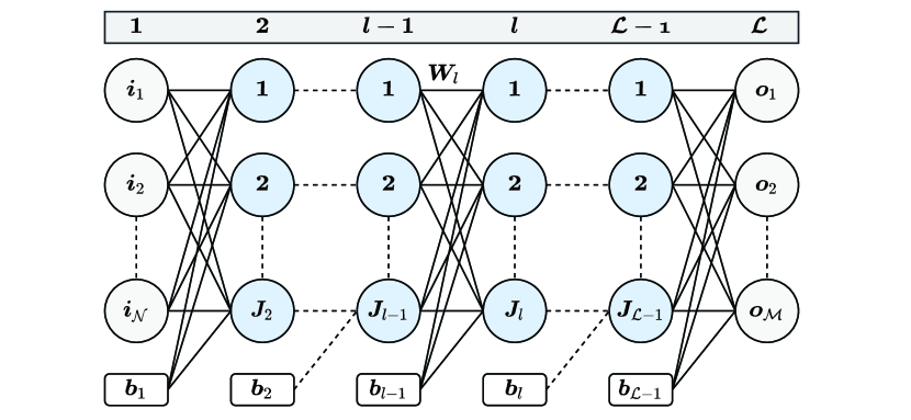
Figure 1: FNN architecture showing the input, output, and hidden layers.

The deep neural network (DNN) overall output of the $l$-th hidden layer is signified by the vector form

$$\bm{o}_{(l)}=\bm{f}_{(l)}\Big{(}\bm{b}_{(l)}+{\bm{W}_{(l)}}\bm{i}_{(l)}\Big{)},\leavevmode\nobreak\ \bm{i}_{(l+1)}=\bm{o}_{(l)},$$ (15)

where $\bm{f}_{(l)}$ is a vector resulting from the stacking of the $n_{l}$ activation functions.

After the selection of the FNN architecture, the parameter ${\theta}=(\bm{W},\bm{B})$ representing the total FNN weights and biases must be estimated via the learning procedure applied during the FNN training phase. As well known, ${\theta}$ estimation is obtained by minimizing a loss function $\text{Loss}({\theta})$. The loss function measures how far apart the predicted FNN outputs ($\bm{o}_{(\mathcal{L})}^{\text{(P)}}$) are from the true outputs ($\bm{o}_{(\mathcal{L})}^{\text{(T)}}$). Therefore, the FNN training phase carried over $N_{\text{train}}$ training samples can be explained in two steps: (i) calculate the loss, and (ii) update ${\theta}$. This process is repeated until convergence, so that the loss becomes very small. Accordingly, various optimization algorithms can be used for minimizing $\text{Loss}({\theta})$ by iteratively updating the parameter ${\theta}$, i.e., stochastic gradient descent [39], root mean square prop [40], and adaptive moment estimation (ADAM) [41].

The final step after FNN training is to test the trained FNN on new data in order to evaluate its performance. An elaborate comprehensive analysis of FNN different principles is presented in [42].

III-B LSTM

Another well-known DL tool is available in the form of LSTM networks that essentially deal with sequential data where the order of the data matters and a correlation exists between the previous and the future data. In this context, LSTM networks are defined with a special architecture capable of learning the data correlation over time, which enables the LSTM network to predict the future data based on prior observations.

The LSTM unit, as shown in Figure 2, contains computational blocks referred to as gates, which are responsible for controlling and tracking the information flow over time. The LSTM network mechanism can be explicated in four major steps:

Forget the irrelevant information

In general, the LSTM unit classifies the input data into relevant and irrelevant information. The first processing step entails eliminating the irrelevant information that is not important for predicting the future. This can be undertaken through the forget gate that decides which information the LSTM unit should retain, and which information can be deleted. The forget gate processing is defined as follows

$${\bm{f}}_{t}=\sigma(\bm{W}_{f,t}\bar{\bm{x}}_{t}+\bm{W}^{\prime}_{f,t}\bar{\bm{z}}_{t-1}+\bar{\bm{b}}_{f,t}),$$ (16)

where $\bar{\sigma}$ denotes the sigmoid function, $\bm{W}_{f,t}\in\mathbb{R}^{P\times K_{in}}$, $\bm{W}^{\prime}_{f,t}\in\mathbb{R}^{P\times P}$ and $\bar{\bm{b}}_{f,t}\in\mathbb{R}^{P\times 1}$ are the forget gate weights and biases at time $t$, $\bar{\bm{x}}_{t}\in\mathbb{R}^{K_{in}\times 1}$ and $\bar{\bm{z}}_{t-1}$ represents the LSTM unit input vector of size $K_{in}$, and the previous hidden state of size $P$, respectively.

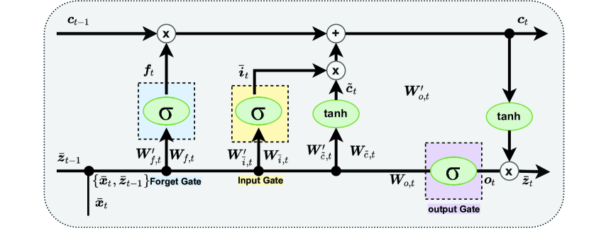
Figure 2: LSTM unit architecture [43].

Store the relevant new information

After classifying the relevant information, the LSTM unit applies some computations on the selected information via the input gate

$${\bar{\bm{i}}_{t}}=\sigma(\bm{W}_{\bar{\bm{i}},t}\bar{\bm{x}}_{t}+\bm{W}^{\prime}_{\bar{\bm{i}},t}\bar{\bm{z}}_{t-1}+\bar{\bm{b}}_{\bar{\bm{i}},t}),$$ (17)

$${\tilde{{\bm{c}}}}_{t}=\text{tanh}(\bm{W}_{{\tilde{{\bm{c}}}},t}\bar{\bm{x}}_{t}+\bm{W}^{\prime}_{{\tilde{{\bm{c}}}},t}\bar{\bm{z}}_{t-1}+\bar{\bm{b}}_{{\tilde{{\bm{c}}}},t}).$$ (18)

Update the new cell state

Next the LSTM unit is supposed to update the current cell state ${{{\bm{c}}}}_{t}$ based on the two previously-mentioned steps such that

$${{{\bm{c}}}}_{t}={\bm{f}}_{t}\odot{\bm{c}}_{t-1}+\bar{\bm{i}}_{t}\odot{\tilde{{\bm{c}}}}_{t}.$$ (19)

where $\odot$ denotes the Hadamard product.

Generate the LSTM unit output

Updating the hidden state and generating the output by the output gate is the final processing step. The output is considered to be a cell state filtered version and can be computed such that

$${\bm{o}}_{t}=\sigma(\bm{W}_{o,t}\bar{\bm{x}}_{t}+\bm{W}^{\prime}_{o,t}\bar{\bm{z}}_{t-1}+\bar{\bm{b}}_{o,t}),$$ (20)

$${\bar{{\bm{z}}}}_{t}={\bm{o}}_{t}\odot\text{tanh}({\bm{c}}_{t}).$$ (21)

In literature, there exists several LSTM architecture variants, where the interactions between the LSTM unit gates are modified. The authors in [44] provide a detailed comparison of popular LSTM architecture variants.

III-C CNN

Another type of deep learning is CNN model. This is commonly used for processing data with grid patterns, such as images [45]. Thus, CNN has generally become the state of the art for several visual applications such as image classification, due to its demonstrated ability to extract patterns from the input image. CNN can be seen as a set of several layers stacked together to accomplish the requisite task. These layers include

• Input layer: It represents the 2D or 3D input image. For the sake of simplicity, let us consider a 2D image input to the $l$ -th CNN layer denoted by $\bm{X}_{l}\in\mathbb{R}^{h_{l}\times w_{l}}$, where $h_{l}$ and $w_{l}$ denote the height and the width of the $\bm{X}_{l}$ input image.

• Convolutional layer: refers to a specialized type of linear operation used for feature extraction, where predefined filters referred to as kernels scan the input matrix to fill the output matrix denoted as feature map, which is shown in Figure 3. We note that different kernels can be considered as different feature extractors.

  Two key hyper parameters define the CNN convolutional layer, namely, the size and number of kernels denoted by $f_{l}$ and $n_{l}$, respectively. The typical kernel size is $3\times 3$, but sometimes $5\times 5$ or $7\times 7$. The number of kernels is arbitrary and determines the depth of output feature maps. It is possible to tune these parameters according to the application type. Furthermore, the process of training a CNN model regarding the convolution layer involves identifying the kernels values that work optimally for a particular task based on a given training dataset. In the convolution layer, the kernels are the only automatically learned parameters during the training process. Mathematically speaking, for a given input image $\bm{X}_{l}$ and kernel $\bm{K_{l}}\in\mathbb{R}^{f_{l}\times f_{l}\times 1}$, we consider one kernel for simplicity, the generated feature map $\bm{Y}_{l}\in\mathbb{R}^{(h_{l}-f+1)\times(w_{l}-f+1)}$ can be expressed as follows

  $$\bm{Y}_{l}[x,y]=\sum^{h_{l}}_{i=1}\sum^{w_{l}}_{j=1}\bm{K}_{l}[i,j]\bm{X}_{l}[x+i-1,y+j-1].$$ (22)

  

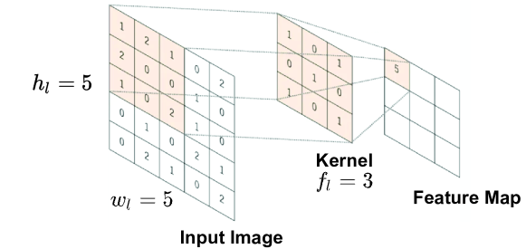
  Figure 3: CNN convolutional layer example [46].

• Activation layer: The outputs of a linear operation such as convolution pass through a nonlinear activation function. This activation function introduces non-linear processing to the CNN architecture given that the input-output CNN pairs relation could be non-linear. While several non-linear activation functions exist such as sigmoid or hyperbolic tangent (tanh) function, the most common presently used function is the rectified linear unit (ReLU).

• Pooling layer: This layer is employed to decrease the number of parameters when the images are too large. Pooling operation is also referred to as sub-sampling or down-sampling. This reduces the dimensionality of all feature maps but does manage to retain significant information. Notably, none of the pooling layers contains any learnable parameter. The most popular form of pooling operation is max pooling, which extracts patches from the input feature maps, outputs the maximum value in each patch, and then discards all the other values. However, there are other pooling operations such as global average pooling [47].

  

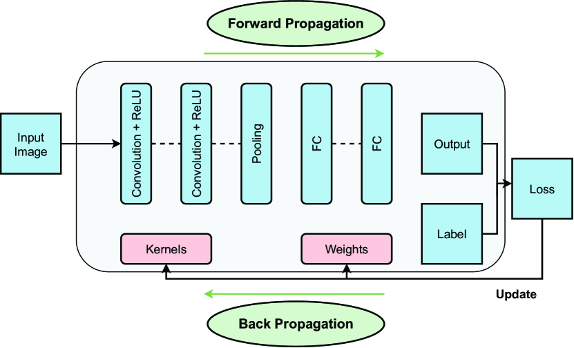
  Figure 4: CNN classical architecture [46].

• Fully connected layer: This layer forms the last block of the CNN architecture and is mainly employed in the classification problems. It is a simple feed-forward neural network layer that comprises at least one hidden layer; its role is to transform the 2D CNN layer output into a 1D vector. In classification problems, the final outputs of the CNN network represent the probabilities for each class, where the final fully-connected layer typically has the same number of output nodes as the number of classes.

• Batch normalization: It is used to increase the CNN stability of the output by normalizing each layer’s output. Moreover, batch normalization layer reduces overfitting and accelerates the CNN training.

• Output layer: This layer is configured in accordance with the studied problem. For instance, in classification problems the CNN output layer is a fully connected layer with softmax activation function. On the other hand, in regression problems, the CNN output does not use any activation function.

Figure 4 illustrates the classical CNN architecture. As seen in this figure, the only trainable parameters within the CNN network are the kernels and the fully connected layer weights. Similar to all other DL techniques, CNN network updates its trainable parameters by minimizing the CNN loss function that measures how far the inputs are from the outputs. Thereafter, the CNN kernels and weights are updated in the back propagation operation [48]. Finally, the performance of the trained CNN model is examined in the testing phase where new unobserved images are fed to the trained CNN model.

It is noteworthy that there are special CNN architectures such as SR-CNN [49], DN-CNN [50], and super resolution convolutional long short-term memory (SR-ConvLSTM) [51] that are mainly used for regression problems. SR-CNN is used for enhancing the quality of the input image, where it takes the low-resolution image as the input and outputs the high-resolution one. DN-CNN uses another methodology to improve the image quality by separating the noise from the input noisy image employing residual learning [52]. The input noisy image is then subtracted from the extracted noise, resulting in the denoised image. Furthermore, SR-ConvLSTM combines both LSTM and CNN networks together where time correlation across the whole input image is learned, thus leading to a better estimation accuracy.

IV DL-Based SBS Channel Estimation

In DL-based SBS channel estimation, FNN and LSTM networks are primarily integrated with conventional estimation schemes in the following two manners: (i) FNN is implemented as a post-processing module after conventional DPA, spectral temporal averaging (STA), and time domain reliable test frequency domain interpolation (TRFI) estimators. (ii) LSTM network gets implemented as a pre-processing unit before conventional DPA estimation to minimize the DPA demapping error iteratively. Both implementations are helpful in improving the channel estimation’s accuracy, particularly in high mobility scenarios. However, the LSTM-based estimation illustrates a considerable superiority over the FNN-based estimation as demonstrated in Section VI. Hereafter, the steps applied in each DL-based SBS estimator are presented.

IV-A DPA-FNN

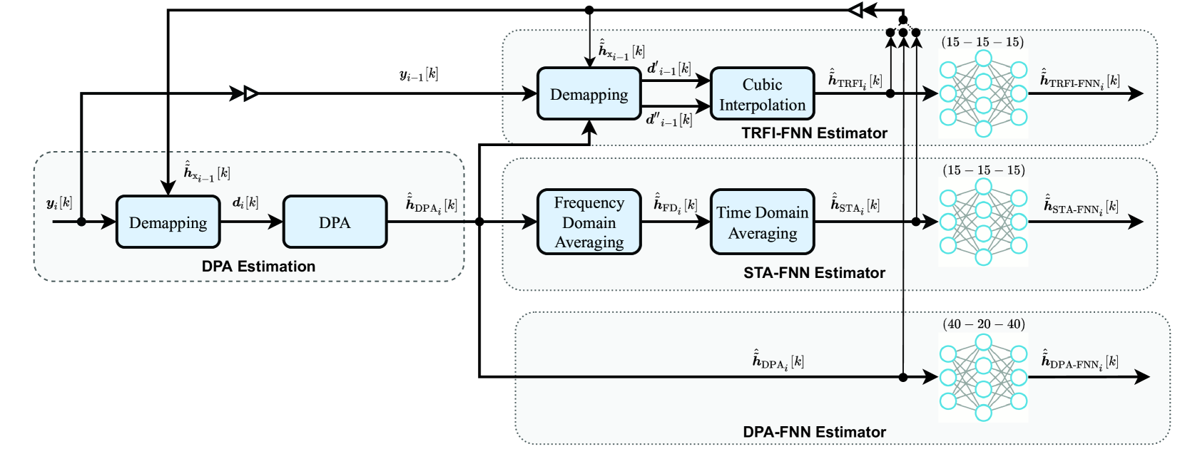
Figure 5: The block diagram of the studied DNN-based SBS estimators.

The DPA estimation [13] utilizes the demapped data subcarriers of the previously received OFDM symbol for estimating the channel for the existing OFDM symbol such that

$$\tilde{\bm{d}}_{i}[k]=\mathfrak{D}\big{(}\frac{\tilde{\bm{y}}_{i}[k]}{\hat{\tilde{\bm{h}}}_{\text{DPA}_{i-1}}[k]}\big{)},\leavevmode\nobreak\ \hat{\tilde{\bm{h}}}_{\text{DPA}_{0}}[k]=\hat{\tilde{\bm{h}}}_{\text{LS}}[k],$$ (23)

where $\mathfrak{D}(.)$ refers to the demapping operation to the nearest constellation point in accordance with the employed modulation order. $\hat{\tilde{\bm{h}}}_{\text{LS}}$ signifies the LS estimated channel at the received preambles, such that

$$\hat{\tilde{\bm{h}}}_{\text{LS}}[k]=\frac{\sum\limits_{u=1}^{P}\tilde{\bm{y}}^{(p)}_{u}[k]}{P\tilde{\bm{\Lambda}}[k]},\leavevmode\nobreak\ k\in{\mathcal{K}}_{\text{on}},$$ (24)

where $\tilde{\bm{\Lambda}}$ denotes the frequency domain predefined preamble sequence. Thereafter, the final DPA channel estimates are updated in the following manner

$$\hat{\tilde{\bm{h}}}_{\text{DPA}_{i}}[k]=\frac{\tilde{\bm{y}}_{i}[k]}{\tilde{\bm{d}}_{i}[k]}.$$ (25)

DPA estimation suffers from two main limitations. First, it is based on the basic $\hat{\tilde{\bm{h}}}_{\text{LS}}$ estimation suffering from noise enhancement. Second, the demapping step in DPA leads to a significant demapping error primarily in low signal-to-noise ratio (SNR) region stemming from the noise imperfections and doubly-dispersive channel variations. This demapping error is enlarged in high mobility scenarios employing high modulation orders. In addition, since the DPA estimated channels are updated iteratively over the received frame, the demapping error propagates via the frame that results in a significant degradation in performance. In order to address these limitations, the DPA-FNN scheme [27] has been proposed to compensate the DPA estimation error, where $\hat{\tilde{\bm{h}}}_{\text{DPA}_{i}}[k]$ is fed to a three-hidden-layers FNN with $40-20-40$ neurons, as shown in Figure 5. Using the FNN in addition to the DPA scheme yields good performance but it is not sufficient, because it ignores the time and frequency correlation between successive received OFDM symbols. Also, the employed FNN architecture can be optimized to reduce the computational complexity of channel estimation.

IV-B STA-FNN

To improve the conventional DPA estimation, the STA estimator [13] has been proposed where frequency and time-domain averaging are applied on top of the DPA estimated channel as follows

$$\hat{\tilde{\bm{h}}}_{\text{FD}_{i}}[k]=\sum_{\lambda=-\beta}^{\lambda=\beta}\omega_{\lambda}\hat{\tilde{\bm{h}}}_{\text{DPA}_{i}}[k+\lambda],\leavevmode\nobreak\ \omega_{\lambda}=\frac{1}{2\beta+1}.$$ (26)

$$\hat{\tilde{\bm{h}}}_{\text{STA}_{i}}[k]=(1-\frac{1}{\alpha})\hat{\tilde{\bm{h}}}_{\text{STA}_{i-1}}[k]+\frac{1}{\alpha}\hat{\tilde{\bm{h}}}_{\text{FD}_{i}}[k].$$ (27)

STA estimator performs well in the low SNR region. However, it suffers from a considerable error floor in high SNR regions due to the large DPA demapping error. Importantly, in [13], the values of the frequency and time averaging coefficients are fixed to $\alpha=\beta=2$. Thus, the final STA estimated channel is a linear combination between the previously estimated channel (27) and the frequency averaged channel estimates (26). However, this linear combination leads to a significant performance degradation in real case scenarios due to the doubly-dispersive channel non-linear imperfections. Here, FNN is utilized as a post non-linear processing unit after the conventional STA scheme [28]. STA-FNN captures more the time-frequency correlations of the channel samples, apart from correcting the conventional STA estimation error. Furthermore, the optimized STA-FNN architecture performs better than the DPA-FNN with a significant computational complexity decrease, as elucidated in Section VII.

IV-C TRFI-FNN

TRFI estimation scheme [15] is another methodology used for improving the DPA estimation in (25). Assuming that the time correlation of the channel response between two adjacent OFDM symbols is high, TRFI define two sets of subcarriers such that: (i) ${\mathcal{RS}}_{i}$ set: that includes the reliable subcarriers indices, and (ii) ${\mathcal{URS}}_{i}$ set: which contains the unreliable subcarriers indices. The estimated channels for the ${\mathcal{URS}}_{i}$ are then interpolated using the ${\mathcal{RS}}_{i}$ channel estimates by means of the frequency-domain cubic interpolation. This procedure can be expressed in the following manner

• Equalize the previously received OFDM symbol by ${\hat{\tilde{\bm{h}}}_{\text{TRFI}_{i-1}}[k]}$ and ${\hat{\tilde{\bm{h}}}_{\text{DPA}_{i}}[k]}$, such that

  $$\begin{split}{\tilde{\bm{d}}^{\prime}}_{i-1}[k]=\mathfrak{D}\big{(}\frac{\tilde{\bm{y}}_{i-1}[k]}{\hat{\tilde{\bm{h}}}_{\text{DPA}_{i}}[k]}\big{)},\leavevmode\nobreak\ {\tilde{\bm{d}}^{\prime\prime}}_{i-1}[k]=\mathfrak{D}\big{(}\frac{\tilde{\bm{y}}_{i-1}[k]}{\hat{\tilde{\bm{h}}}_{\text{TRFI}_{i-1}}[k]}\big{)}.\end{split}$$ (28)

• According to the demapping results, the subcarriers are grouped as follows

  $$\left\{\begin{array}[]{ll}{\mathcal{RS}}_{i}\leftarrow{\mathcal{RS}}_{i}+{k},&\quad\tilde{\bm{d^{\prime}}}_{i-1}[k]=\tilde{\bm{d}}^{\prime\prime}_{i-1}[k]\\ {\mathcal{URS}}_{i}\leftarrow{\mathcal{URS}}_{i}+{k},&\quad\tilde{\bm{d^{\prime}}}_{i-1}[k]\neq\tilde{\bm{d}}^{\prime\prime}_{i-1}[k]\end{array}\right..$$ (29)

• Finally, frequency-domain cubic interpolation is employed to estimate the channels at the ${\mathcal{URS}}_{i}$ as follows

  $$\hat{\tilde{\bm{h}}}_{\text{TRFI}_{i}}[k]=\left\{\begin{array}[]{ll}\hat{\tilde{\bm{h}}}_{\text{DPA}_{i}}[k],&\quad k\in{\mathcal{RS}}_{i}\\ \text{Cubic Interpolation},&\quad k\in{\mathcal{URS}}_{i}\end{array}\right..$$ (30)

Performing frequency-domain interpolation in addition to the DPA estimation enhances the performance. However, TRFI still suffers from the demapping and interpolation errors as the number of reliable subcarriers (RS) subcarriers is inversely proportional to the channel variations. Additionally, the condition where ${\tilde{\bm{d}}^{\prime}}_{i-1}[k]\neq{\tilde{\bm{d}}^{\prime\prime}}_{i-1}[k]$ is more dominant in high mobility scenarios. It is for this reason that only a few RS subcarriers will be selected and the employed cubic interpolation performance will be degraded.

Inspired by the work undertaken in STA-FNN, the authors in [29] used the same optimized FNN architecture as in [28], albeit with $\hat{\tilde{\bm{h}}}_{\text{TRFI}_{i}}[k]$ as an input instead of $\hat{\tilde{\bm{h}}}_{\text{STA}_{i}}[k]$. TRFI-FNN corrects the cubic interpolation error and also learns the channel frequency domain correlation, thus leading to an improved performance in high SNR regions.

IV-D LSTM-FNN-DPA

Unlike the FNN-based estimators, where the DL processing is employed following the conventional estimators, the work carried out in [53] shows that employing the DL processing prior to the conventional estimator, specifically the DPA estimation, could lead to a significant improvement in the overall performance. In this context, the authors have proposed to use two cascaded LSTM and FNN networks for both channel estimation as well as noise compensation, as shown in Figure 6.

The LSTM-FNN-DPA estimator employs the previous and current pilot subcarriers besides the LSTM-FNN estimated channel employed in the DPA estimation, such that

$$\tilde{\bm{d}}_{\text{LSTM-FNN}_{i,d}}[k]=\mathfrak{D}\big{(}\frac{\tilde{\bm{y}}_{i,d}[k]}{\hat{\tilde{\bm{h}}}_{\text{LSTM-FNN}_{i-1,d}}[k]}\big{)},\leavevmode\nobreak\ \hat{\tilde{\bm{h}}}_{\text{LSTM}_{0}}[k]=\hat{\tilde{\bm{h}}}_{\text{LS}}[k],$$ (31)

$$\hat{\tilde{\bm{h}}}_{\text{DL}_{i,d}}[k]=\frac{\tilde{\bm{y}}_{i,d}[k]}{\bm{d}_{\text{LSTM}_{i,d}}[k]}.$$ (32)

While this estimator can outperform the FNN-based estimators, it experiences a considerable computational complexity arising from the employment of two DL networks.

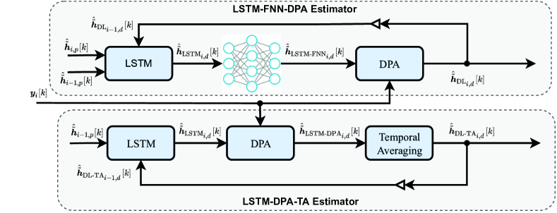
Figure 6: The block diagram of the studied LSTM-based SBS estimators.

IV-E LSTM-DPA-TA

The authors in [43] propose to use only LSTM network instead of two as implemented in the LSTM-FNN-DPA estimator. In addition, noise compensation is made possible by applying time averaging (TA) processing as shown in Figure 6. This methodology only requires the previous pilots besides the LSTM estimated channel as an input. Then, the LSTM estimated channel is employed in the DPA estimation as follows

$$\tilde{\bm{d}}_{\text{LSTM}_{i}}[k]=\mathfrak{D}\big{(}\frac{\tilde{\bm{y}}_{i}[k]}{\hat{\tilde{\bm{h}}}_{\text{LSTM}_{i-1}}[k]}\big{)},\leavevmode\nobreak\ \hat{\tilde{\bm{h}}}_{\text{LSTM}_{0}}[k]=\hat{\tilde{\bm{h}}}_{\text{LS}}[k],$$ (33)

$$\hat{\tilde{\bm{h}}}_{\text{LSTM-DPA}_{i}}[k]=\frac{\tilde{\bm{y}}_{i}[k]}{\tilde{\bm{d}}_{\text{LSTM}_{i}}[k]}.$$ (34)

Finally, to alleviate the impact of the AWGN noise, TA processing is applied to the $\hat{\tilde{\bm{h}}}_{\text{LSTM-DPA}_{i}}[k]$ estimated channel, such that

$$\hat{\bar{\bm{h}}}_{\text{DL-TA}_{i,d}}=(1-\frac{1}{\alpha})\hat{\bar{\bm{h}}}_{\text{DL-TA}_{i-1,d}}+\frac{1}{\alpha}\hat{\bar{\bm{h}}}_{\text{LSTM-DPA}_{i,d}}.$$ (35)

Here, $\alpha$ denotes the utilized weighting coefficient. In [43], the authors use a fixed $\alpha=2$ for simplicity. Therefore, the TA applied in (35) reduces the AWGN noise power $\sigma^{2}$ iteratively within the received OFDM frame according to the ratio

$$\begin{split}{R}_{\text{DL-TA}_{q}}&=\left(\frac{1}{4}\right)^{(q-1)}+\sum_{j=2}^{q}\left(\frac{1}{4}\right)^{(q-j+1)}=\frac{4^{q-1}+2}{3\times 4^{q-1}}.\end{split}$$ (36)

This corresponds to the AWGN noise power ratio of the estimated channel at the $q$-th estimated channel, where ${1<q<I+1}$ and ${{R}_{\text{DL-TA}_{1}}=1}$ denotes the AWGN noise power ratio at $\hat{\tilde{\bm{h}}}_{\text{LS}}[k]$. From the derivation of ${R}_{\text{DL-TA}_{q}}$, it can be seen that the noise power decreases over the received OFDM frame, i.e., the SNR increases, resulting in an overall improved performance. Moreover, the input dimension reduction, coupled with the simple TA processing, significantly lowers the overall computational complexity.

Table I: Parameters of the studied DL-based SBS channel estimators.

DPA-FNN (Hidden layers; Neurons per layer)	(3;40-20-40)
STA-FNN (Hidden layers; Neurons per layer)	(3;15-15-15)
TRFI-FNN (Hidden layers; Neurons per layer)	(3;15-15-15)
LSTM (Hidden layers; Neurons per layer)	(1;128)
Activation function	ReLU
Number of epochs	500
Training samples	800000
Testing samples	200000
Batch size	128
Optimizer	ADAM
Loss function	MSE
Learning rate	0.001
Training SNR	40 dB

Intensive experiments reveal that the performance of DL networks is strongly related to the SNR considered in the training [54]. The training undertaken at the highest SNR value provides the best performance. In fact, the DL network is able to learn better the channel when the training is performed at a high SNR value because the impact of the channel is higher than the impact of the noise in this SNR range. Owing to the robust generalization properties of DL, trained networks can still estimate the channel even if the noise increases, i.e., at low SNR values. Therefore, FNN and LSTM based estimators training is performed using SNR = $40$ dB to attain the best performance. Moreover, intensive experiments are performed using the grid search algorithm [55] to select the most suitable FNN and LSTM hyper parameters in terms of performance as well as complexity. Figures 5 and 6 illustrate the block diagram of the FNN and LSTM based estimators. Furthermore, Table I presents their parameters.

V DL-Based FBF Channel Estimation Schemes

This section presents the DL-based FBF estimators introduced to improve the channel estimation accuracy, particularly in very high mobility scenarios, where the channel variation is found to be severe. Similar to the DL-based SBS estimators, the DL-based FBF estimators apply first conventional estimation followed by means of CNN processing.

Table II: Main characteristics and features of the studied DL-based channel estimators.

Estimator type	Estimator reference	Conventional estimation	DL-based Method	Complexity	BER Performance	Robustness	Pros and Cons
SBS	[27]	DPA	FNN	++	++	++	+ Significant performance superiority over conventional estimators. - Ignore the time and frequency correlation between successive received OFDM symbols. - Complex FNN architecture to compensate the conventional DPA demapping error.
	[28]	STA		+	+++	++	+ STA averaging ameliorate the impact of the AWGN noise in low SNR regions. + Optimized FNN architecture. - Fixed averaging coefficients. - Performance degradation in high mobility scenarios.
	[29]	TRFI		+	++++	+++	+ Cubic Interpolation enhances the performance in the entire SNR region. + Optimized FNN architecture. - Assume high correlation between successive OFDM symbols. - Lack of robustness in very high mobiliy scenarios.
	[53]	DPA	LSTM and FNN	+++	++++	++++	+ Outperform FNN-based estimators. + Improved estimation since LSTM is implemented before DPA estimation - Employ LSTM and FNN in the same architecture.
	[43]	DPA and TA	LSTM	+++	++++	++++	+ TA processing results in a considerable decline in the AWGN noise. + Employ only one optimized LSTM unit. + Reduced input dimension.
FBF	[30]	2D RBF	SR-CNN and DN-CNN	+++++	++	++	- 2D RBF interpolation high computational complexity. - The 2D RBF function and scale factor should be optimized in accordance with the channel variations. - Employ two high-complexity CNN architectures.
	[31]	ADD-TT	SR-ConvLSTM	+++++	+++	+++	+ Outperform ChannelNet estimator [29]. - Fixed ADD-TT Averaging coefficients. - High computational complexity owing to the integration of both LSTM and CNN architectures.
	[32]	WI	SR-CNN or DN-CNN	+++	++++	++++	+ Adaptive frame structure according to the mobility condition. + Reduced buffering time at the receiver. + Transmission data rate gain. + Optimized CNN architectures.

V-A ChannelNet

In [30], the authors use forward a CNN-based channel estimator denoted as channel network (ChannelNet) scheme, where 2D radial basis function (RBF) interpolation is implemented as an initial channel estimation. The underlying motivation of the 2D RBF interpolation is to approximate multidimensional scattered unknown data from their surrounding neighbors known data by employing the radial basis function. In order to achieve the purpose, the distance function is calculated between every data point to be interpolated and its neighbours, where closer neighbors are assigned higher weights. Thereby, the RBF interpolated frame is considered a low resolution image, where SR-CNN is utilized to obtain an improved estimation. Finally, to ameliorate the effect of noise within the high resolution estimated frame, DN-CNN is implemented leading to a high resolution and noise alleviated estimated channels. The ChannelNet estimator considers sparsely allocated pilots within the IEEE 802.11p frame and initially applies the LS estimation to the pilot subcarriers within the received OFDM frame. Subsequently, the 2D RBF interpolation is derived by the weighted summation of the distance between each data subcarrier to be interpolated as well as all the pilot subcarriers in the received OFDM frame, such that

$$\hat{\tilde{\bm{H}}}_{\text{RBF}}[k,i]=\sum_{j=1}^{{K_{{p}}}I}\omega_{j}\Phi(|k-{\mathcal{K}}_{f}[j]|,|i-{\mathcal{K}}_{t}[j]|).$$ (37)

${\mathcal{K}}_{f}=[{{\mathcal{K}}}_{\text{p}_{1}},\dots,{{\mathcal{K}}}_{\text{p}_{I}}]\in\mathbb{R}^{1\times K_{p}I}$ and ${\mathcal{K}}_{t}=[(1)_{\times K_{p}},\dots,(I)_{\times K_{p}}]\in\mathbb{R}^{1\times K_{p}I}$ represent the frequency and time indices vectors of the allocated pilot subcarriers within the received OFDM frame, respectively. $\omega_{j}$ is the RBF weight multiplied by the RBF interpolation function $\Phi(.)$ between the $(k,i)$ data subcarrier and the $({\mathcal{K}}_{f}[j],{\mathcal{K}}_{t}[j])$ pilot subcarrier. In [30], the RBF gaussian function is applied, such that

$$\Phi(x,y)=e^{-\frac{(x+y)^{2}}{r_{0}}}.$$ (38)

$r_{0}$ refers to the 2D RBF scale factor that varies based on the used RBF function. Notably, altering the value of $r_{0}$ alters the shape of the interpolation function. Moreover, the RBF weights $\bm{w}_{\text{RBF}}=[\omega_{1},\dots,\omega_{K_{p}I}]\in\mathbb{R}^{K_{p}I\times 1}$ are calculated using the following relation:

$$\bm{A}_{\text{RBF}}\bm{w}_{\text{RBF}}=\bar{{\bm{h}}}_{\text{LS}}.$$ (39)

Here, $\bm{A}_{\text{RBF}}\in\mathbb{R}^{{K_{{p}}}I\times{K_{{p}}}I}$ is the RBF interpolation matrix of the pilots subcarriers, with entries $a_{i,j}=\Phi({\mathcal{K}}_{f}[i],{\mathcal{K}}_{t}[j])$ where $i,j=1,\dots,K_{p}I$. It is observed that, $\bar{{\bm{h}}}_{\text{LS}}=\mathrm{vec}\left\{\hat{\tilde{\bm{H}}}_{\text{LS}}\right\}\in\mathbb{C}^{K_{p}I\times 1}$ is a vector that contains the LS estimated channels at all the pilot subcarriers within the received OFDM frame. This is expressed as

$$\hat{\tilde{\bm{H}}}_{\text{LS}}[k,i]=\frac{\tilde{\bm{Y}}[k,i]}{\tilde{\bm{P}}[k,i]},\leavevmode\nobreak\ k\in{{\mathcal{K}}}_{\text{p}},\leavevmode\nobreak\ 1\leq i\leq I,$$ (40)

with $\tilde{\bm{P}}[k,i]$ is the frequency-domain pre-defined pilot subcarriers, and ${{\mathcal{K}}}_{\text{p}}$ refers to the allocated sparse pilots indices within the received OFDM symbol. After computing $\bm{W}_{\text{RBF}}$, it is possible to calculate the RBF estimated channel for every data subcarriers within the received OFDM frame, as shown in (37). Finally, the RBF interpolation estimated frame $\hat{\tilde{\bm{H}}}_{\text{RBF}}$ is fed as an input to SR-CNN and DN-CNN to improve the channel estimation accuracy and reduce the noise impact.

The ChannelNet estimator limitations lie in: (i) 2D RBF interpolation high computational complexity arising from the computation of (39) for the channel estimation of all data subcarriers. (ii) The 2D RBF function and scale factor needs to be optimized in accordance with the channel variations. (iii) The integrated SR-CNN and DN-CNN architectures have significant computational complexity. Notably, the ChannelNet estimator uses a fixed RBF function and scale factor, thus experiencing a considerable degradation in performance, particularly in low SNR regions, where the noise impact remains dominant, as well as high mobility vehicular scenarios, where the channel varies swiftly within the OFDM frame.

Table III: Parameters of the studied DL-based FBF channel estimators.

Parameter	Values
Input/Output dimensions	$2K_{\text{on}}\times I\times 1$
SR-CNN (Hidden layers - $n_{l},f_{l}$)	(3 - 9,64; 1,32;  5,1)
DN-CNN (Hidden layers - $n_{l},f_{l}$)	(18 - 64, 3)
Optimized SR-CNN (Hidden layers - $n_{l},f_{l}$)	(3 - 9,32; 1,16;  5,1)
Optimized DN-CNN (Hidden layers - $n_{l},f_{l}$)	(7 - 16, 3)
SR-ConvLSTM (Hidden layers - $n_{l},f_{l}$)	(3 - 9,64; 1,32;  5,1)
Activation function	ReLU
Number of epochs	250
Training samples	8000
Testing samples	2000
Batch size	128
Optimizer	ADAM
Loss function	MSE
Learning rate	0.001
Training SNR	40 dB

V-B TS-ChannelNet

Temporal spectral ChannelNet (TS-ChannelNet) [31] is based on applying average decision-directed with time truncation (ADD-TT) interpolation to the received OFDM frame. Thereafter, accurate estimation is achieved by implementing SR-ConvLSTM network to track doubly-dispersive channel variations by learning the vehicular channel’s time and frequency correlations. It is observed that the ADD-TT interpolation is an SBS estimator, where DPA estimation is initially applied as explained in (23) and (25). Thereafter, the enlarged DPA demapping error is reduced by applying time domain truncation in the following manner

$$\hat{{\bm{h}}}_{\text{DPA}_{i}}={\bm{F}}_{\text{K}}^{\text{H}}\hat{\tilde{\bm{h}}}_{\text{DPA}_{i}},$$ (41)

where ${\bm{F}}_{K}\in\mathbb{C}^{K\times K}$ denotes the $K$-DFT matrix, and $\hat{{\bm{h}}}_{\text{DPA}_{i}}$ represents the time-domain DPA estimated channel. Thereafter, $\hat{{\bm{h}}}_{\text{DPA}_{i}}$ truncation is applied to the significant $L$ channel taps, such that

$$\hat{{\bm{h}}}_{\text{DPA}_{i,L}}=\hat{{\bm{h}}}_{\text{DPA}_{i}}(1\mathrel{\mathop{\mathchar 58\relax}}L).$$ (42)

Next, $\hat{{\bm{h}}}_{\text{DPA}_{i,L}}$ is converted back to the frequency domain such that

$$\hat{\tilde{\bm{h}}}_{\text{TT}_{i}}={\bm{F}}_{\text{K}}\hat{{\bm{h}}}_{\text{DPA}_{i,L}},$$ (43)

Implementing the average time truncation operation to $\hat{\tilde{\bm{h}}}_{\text{DPA}_{i}}[k]$ lowers the effect of noise and enlarged demapping error. Moreover, $\hat{\tilde{\bm{h}}}_{\text{TT}_{i}}[k]$ estimated channel is further enhanced by applying frequency and time-domain averaging consecutively as follows

$$\hat{\tilde{\bm{h}}}_{\text{FTT}_{i}}[k]=\sum_{\lambda=-\beta}^{\lambda=\beta}\omega_{\lambda}\hat{\tilde{\bm{h}}}_{\text{TT}_{i}}[k+\lambda],\leavevmode\nobreak\ \omega_{\lambda}=\frac{1}{2\beta+1}.$$ (44)

The final ADD-TT channel estimates are updated using time averaging between the previously ADD-TT estimated channel and the frequency averaged channel in (44), such that

$$\hat{\tilde{\bm{h}}}_{\text{ADD-TT}_{i}}[k]=(1-{\alpha})\hat{\tilde{\bm{h}}}_{\text{ADD-TT}_{i-1}}[k]+{\alpha}\hat{\tilde{\bm{h}}}_{\text{FTT}_{i}}[k].$$ (45)

The doubly-dispersive channel can be modeled as a time-series forecasting problem. Here, historical data can be utilized to forecast future observations [56]. Motiviated by this possibility, the authors in [31] apply SR-ConvLSTM network in addition to the ADD-TT interpolation, where convolutional layers get added to the LSTM network to capture more doubly-dispersive channel features. Consequently, this improves the estimation performance. Accordingly, the ADD-TT estimated channel for the entire received frame is modeled as a low resolution image. Next, the SR-ConvLSTM network is used after the ADD-TT interpolation. Unlike ChannelNet estimator where two CNNs are employed, TS-ChannelNet estimator uses only one SR-ConvLSTM network, which relatively reduces the overall computational complexity. However, TS-ChannelNet continues to be ridden with high computational complexity due to the integration of LSTM and CNN in a single network.

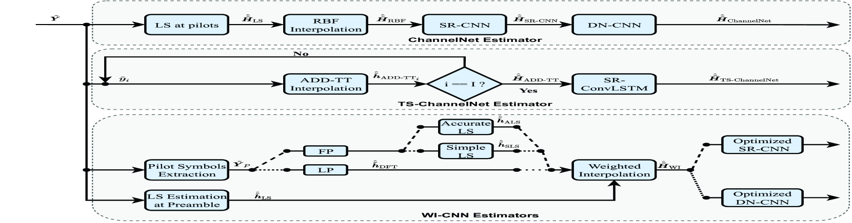
Figure 7: The block diagram of the studied CNN-based FBF channel estimators.

V-C WI-CNN

To overcome the limitations of the ChannelNet and TS-ChannelNet estimators, weighted interpolation (WI)-CNN estimator has been proposed in [32]. In this method, the frame structure is adapted in accordance with the mobility condition employing varied pilot allocation schemes. Particularly, only $P$ pilot OFDM symbols are required in the transmitted frame, such that $\tilde{\bm{Y}}_{P}=[\tilde{\bm{y}}^{(p)}_{1},\dots,\tilde{\bm{y}}^{(p)}_{q},\dots,\tilde{\bm{y}}^{(p)}_{P}]\in\mathbb{C}^{K_{\text{on}}\times P}$. The index $1\leq q\leq P$ refers to the location of the OFDM pilot symbol in the frame. The other $I_{d}=I-P$ OFDM data symbols are employed for data transmission purposes. As per the employed pilots allocation scheme, the channel is estimated at the inserted pilot symbols, after which WI is applied to estimate the channel at the OFDM data symbols. The estimated frame is then modeled as a 2D noisy image where optimized SR-CNN and DN-CNN are utilized for noise elimination. Against this backdrop, the WI-CNN proceeds as follows

• Channel estimation at the pilot symbols: Two pilot allocation schemes are defined. The full pilot allocation (FP) where $K$ pilots are inserted within all pilot symbols and LS estimation is applied to estimate the channel for each inserted pilot symbol, such that

  $$\hat{\tilde{\bm{h}}}_{{\text{SLS}}_{q}}[k]=\frac{\tilde{\bm{y}}^{(p)}_{q}[k]}{\tilde{\bm{p}}[k]}.$$ (46)

  $\hat{\tilde{\bm{h}}}_{{\text{SLS}}_{q}}[k]$ represents the simple LS (SLS) estimation at the $q$-th inserted pilot symbol. In addition, the accurate LS (ALS) that can be obtained by implementing the DFT interpolation of estimated channel impulse response at the $q$-th received pilot symbol $\hat{\bm{h}}_{q,L}$, such that

  $$\hat{\tilde{\bm{h}}}_{{\text{ALS}}_{q}}=\bm{F}_{\text{K}}\hat{\bm{h}}_{q,L},\leavevmode\nobreak\ \leavevmode\nobreak\ \hat{\bm{h}}_{q,L}=\bm{F}_{\text{K}}^{\dagger}\hat{\tilde{\bm{h}}}_{{\text{LS}}_{q}}.$$ (47)

  ALS relies on the fact that $\tilde{\bm{h}}_{{q}}=\bm{F}_{\text{K}}{\bm{h}}_{q,L}$, where ${\bm{h}}_{q,L}\in\mathbb{C}^{L\times 1}$ signifies the channel impulse response at the $q$-th received pilot symbol that can be estimated by employing the pseudo inverse matrix of $\bm{F}_{\text{K}}$, namely, $\bm{F}_{\text{K}}^{\dagger}=[(\bm{F}_{\text{K}}^{\text{H}}\bm{F}_{\text{K}})^{-1}\bm{F}_{\text{K}}^{\text{H}}]$ . However, if the number of doubly dispersive-channel taps $L$ remains known, only $K_{p}=L$ pilot subcarriers are sufficient in each inserted pilot symbol. Accordingly, (47) can be rewritten as

  $$\hat{\tilde{\bm{h}}}_{{\text{DFT}}_{q}}=\bm{F}_{\text{K}}\hat{\bm{h}}_{q,L},\leavevmode\nobreak\ \leavevmode\nobreak\ \hat{\bm{h}}_{q,L}=\bm{F}_{p}^{\dagger}\hat{\tilde{\bm{h}}}_{{\text{LS}}_{q}}.$$ (48)

  $\bm{F}_{p}^{\dagger}=[(\bm{F}_{p}^{\text{H}}\bm{F}_{p})^{-1}\bm{F}_{p}^{\text{H}}]$ denotes the pseudo inverse matrix of $\bm{F}_{p}\in\mathbb{C}^{K_{\text{p}}\times L}$ referring to the truncated DFT matrix obtained by selecting ${\mathcal{K}}_{\text{p}}$ rows, and $L$ columns from the $K$-DFT matrix.

• Channel estimation at data symbols: The estimated channels of the $P$ pilot symbols are first grouped into $P$ matrices to estimate the channel for each received OFDM data symbol, such that

  $$\hat{\tilde{\bm{H}}}_{q}=[\hat{\tilde{\bm{h}}}_{q-1},\hat{\tilde{\bm{h}}}_{q}],\leavevmode\nobreak\ q=1,\cdots P.$$ (49)

  $\hat{\tilde{\bm{h}}}_{0}=\hat{\tilde{\bm{h}}}_{\text{LS}}$ refers to the LS estimated channel at the beginning of the received frame (24). Thus, the received frame can be divided into $P$ sub-frames, where $f$ refers to the sub-frame index, such that $1\leq f\leq P$. Therefore, the estimated channel for the $i$-th received OFDM symbol within each $f$-th sub-frame can be expressed as follows

  $$\hat{\tilde{\bm{H}}}_{{\text{WI}}_{f}}=\hat{\tilde{\bm{H}}}_{{f}}\bm{C}_{f}.$$ (50)

  $\hat{\tilde{\bm{H}}}_{f}\in\mathbb{C}^{K\times 2}$ denotes the LS estimated channels at the pilot symbols within the $f$-th sub-frame, and $\bm{C}_{f}\in\mathbb{R}^{2\times I_{f}}$ the interpolation weights of the $I_{f}$ OFDM data symbols within the $f$-th sub-frame. The interpolation weights $\bm{C}_{f}$ are calculated by minimizing the mean squared error (MSE) between the ideal channel $\tilde{\bm{H}}_{{f}}$, and the LS estimated channel at the OFDM pilot symbols $\hat{\tilde{\bm{H}}}_{{f}}$ as obtained in [57] and expressed in (51). There, $J_{0}(.)$ is the zeroth order Bessel function of the first kind, $T_{\text{s}}$ signifies the received OFDM data symbol duration, whereas $E_{{{q}}}$ denotes the overall noise of the estimated channel at the $q$-th pilot symbol.

  $$\begin{split}\bm{C}_{{f}}&=\mathrm{E}\left[\tilde{\bm{H}}_{{f}}\hat{\tilde{\bm{H}}}^{H}_{{f}}\right]\left[\mathrm{E}\left[\hat{\tilde{\bm{H}}}_{{f}}\hat{\tilde{\bm{H}}}^{H}_{{f}}\right]\right]^{-1}=\begin{bmatrix}\mathrm{E}\left[\tilde{\bm{H}}_{{f}}\hat{\tilde{\bm{h}}}^{H}_{{q}}\right]&\mathrm{E}\left[\tilde{\bm{H}}_{{i}}\hat{\tilde{\bm{h}}}^{H}_{{q+1}}\right]\end{bmatrix}\begin{bmatrix}\mathrm{E}\left[\mathinner{\!\left\lVert{\tilde{\bm{h}}}_{{q}}\right\rVert}^{2}\right]+E_{{{q}}}&\mathrm{E}\left[{\tilde{\bm{h}}}_{{q}}{\tilde{\bm{h}}}^{H}_{{q+1}}\right]\\ \mathrm{E}\left[{\tilde{\bm{h}}}_{{q+1}}{\tilde{\bm{h}}}^{H}_{{q}}\right]&\mathrm{E}\left[\mathinner{\!\left\lVert{\tilde{\bm{h}}}_{{q+1}}\right\rVert}^{2}\right]+E_{{{q+1}}}\end{bmatrix}^{-1}\\ &=\begin{bmatrix}J_{0}(2\pi f_{\text{d}}(f-1)T_{\text{s}})&J_{0}(2\pi f_{\text{d}}(I_{f}+1-f)T_{\text{s}})\end{bmatrix}\begin{bmatrix}1+E_{{{\Phi}_{q}}}&J_{0}(2\pi f_{\text{d}}I_{f}T_{\text{s}})\\ J_{0}(2\pi f_{\text{d}}I_{f}T_{\text{s}})&1+E_{{{q+1}}}\end{bmatrix}^{-1}.\end{split}$$ (51)

• CNN-based Processing: The final step in the WI-CNN estimators is to apply CNN processing to further improve the WI estimated channels. Optimized SR-CNN and DN-CNN are employed in this context. The investigations conducted in [32] reveal that both SR-CNN and DN-CNN networks have similar performance in low mobility scenarios, whereas DN-CNN outperforms SR-CNN in high mobility scenarios. Figure 7 and Table III illustrate the block diagram as well as configured parameters of the studied CNN-based channel estimators, respectively. Furthermore, the salient features of the studied DL-based channel estimators are summarized in Table II. Notably, robustness feature alludes to the ability of the studied estimation to maintain good performance as the variation of the doubly-dispersive channel increases.

Table IV: The characteristics of the employed vehicular channel models following Jake’s Doppler spectrum.

Channel model	Channel taps	Vehicle velocity [kmph]	Doppler shift [Hz]	Average path gains [dB]	Path delays [ns]
VTV-UC	12	45	250	[0, 0, -10, -10, -10, -17.8, -17.8, -17.8, -21.1, -21.1, -26.3, -26.3]	[0, 1, 100, 101, 102, 200, 201, 202, 300, 301, 400, 401]
VTV-SDWW	12	100-200	500-1000	[0, 0, -11.2, -11.2, -19, -21.9, -25.3, -25.3, -24.4, -28, -26.1, -26.1]	[0, 1, 100, 101, 200, 300, 400, 401, 500, 600, 700, 701]

VI Simulation Results

This section illustrates the performance evaluation of the studied DL-based SBS and FBF estimators in relation to BER, NMSE employing varied metrics and mobility scenarios.

VI-A Configuration Setup

To simulate doubly-dispersive channels, vehicular communications is considered a simulation case study, where three tapped delay line (TDL) channel models [58] are defined as follows

• Low mobility: where VTV Urban Canyon (VTV-UC) vehicular channel model is considered. This channel model is measured between two vehicles moving in a dense urban traffic environment at ${V}=45$ Kmph equivalent to ${f}_{d}=250$ Hz.

• High and very high mobility: These scenarios measure the communication channel between two vehicles moving on a highway having center wall between its lanes at ${V}=100$ Kmph and $200$ Kmph equivalent to ${f}_{d}=500$ Hz and ${f}_{d}=1000$ Hz, respectively. This vehicular channel model is referred to as VTV Expressway Same Direction with Wall (VTV-SDWW).

The employed channel models are generated after the wide-sense stationary uncorrelated scattering (WSSUS) model [59]. Thus, we have

• Each path $h_{l}(t)$ is a zero mean Gaussian complex process, $E\{h_{l}(t)\}=0,\forall t$, and the mean of each path is independent of the time variations. Moreover, the time correlation function $r_{h_{l}}(t_{1},t_{2})=E\{h_{l}(t_{1})h^{*}_{l}(t_{2})\}$ can only be written with the difference $\Delta(t)=(t_{1}-t_{2})$, such that

  $$r_{h_{l}}(t_{1},t_{2})=r_{h_{l}}(\Delta_{t}).$$ (52)

  Then, each path $h_{l}(t)$ is the wide sense stationary (WSS).

• Uncorrelated scattering (US) implies that the paths are uncorrelated, so for $l_{1}\neq l_{2}$ we have

  $$\small E[h_{l_{1}}(t)h^{*}_{l_{2}}(t)]=0.$$ (53)

Table IV illustrates the main characteristics of the defined TDL channel models.

The OFDM simulation parameters are based on the IEEE 802.11p standard as illustrated in Table V. These simulations are implemented using QPSK and 16QAM modulation orders, the SNR range is $[0,5,\dots,40]$ dB. In addition, the performance evaluation is made according to: (i) modulation order, (ii) mobility, (iii) frame length, and (iv) DL architecture.

Finally, it is observed that the conventional 2D LMMSE estimator [17] is included in the performance evaluation of the DL-based FBF estimators as a lower bound performance limit. The 2D LMMSE estimator almost achieves a similar performance as the ideal channel, but is ridden with high computational complexity. This renders it impractical in terms of real-time applications.

Table V: Simulation parameters of the IEEE 802.11p physical layer.

Parameter	IEEE 802.11p
Bandwidth	10 MHz
Guard interval duration	1.6 $\mu\mbox{s}$
Symbol duration	8 $\mu\mbox{s}$
Short training symbol duration	1.6 $\mu\mbox{s}$
Long training symbol duration	6.4 $\mu\mbox{s}$
Total subcarriers	64
Pilot subcarriers	4
Data subcarriers	48
Subcarrier spacing	156.25 KHz

VI-B DL-Based SBS Estimation Schemes

VI-B1 Modulation Order

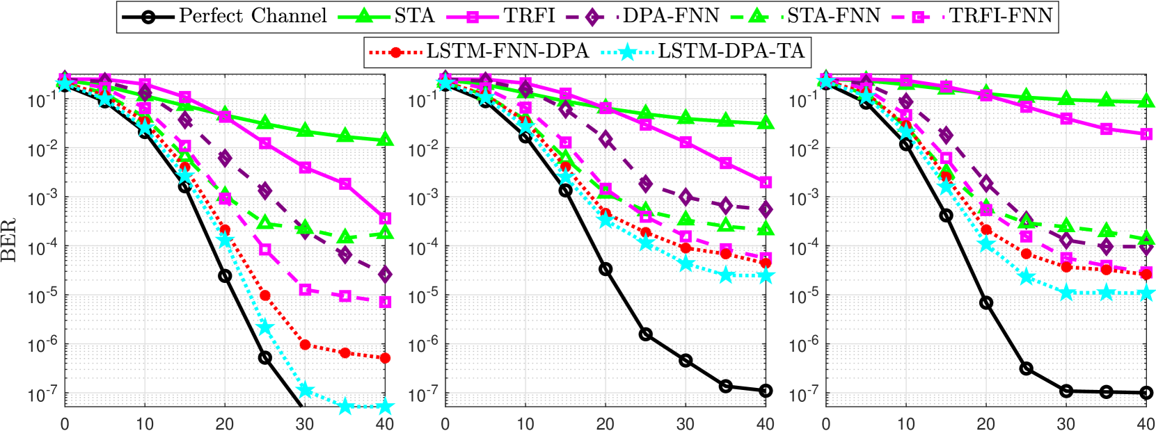
(a)

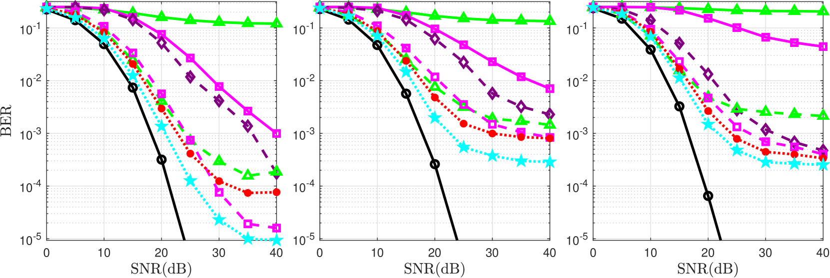
(b)

Figure 8: BER for $I=100$, mobility from left to right: low ($v=45\leavevmode\nobreak\ \text{Kmph},f_{d}=250$ Hz), high ($v=100\leavevmode\nobreak\ \text{Kmph},f_{d}=500$ Hz), very high ($v=200\leavevmode\nobreak\ \text{Kmph},f_{d}=1000$ Hz).

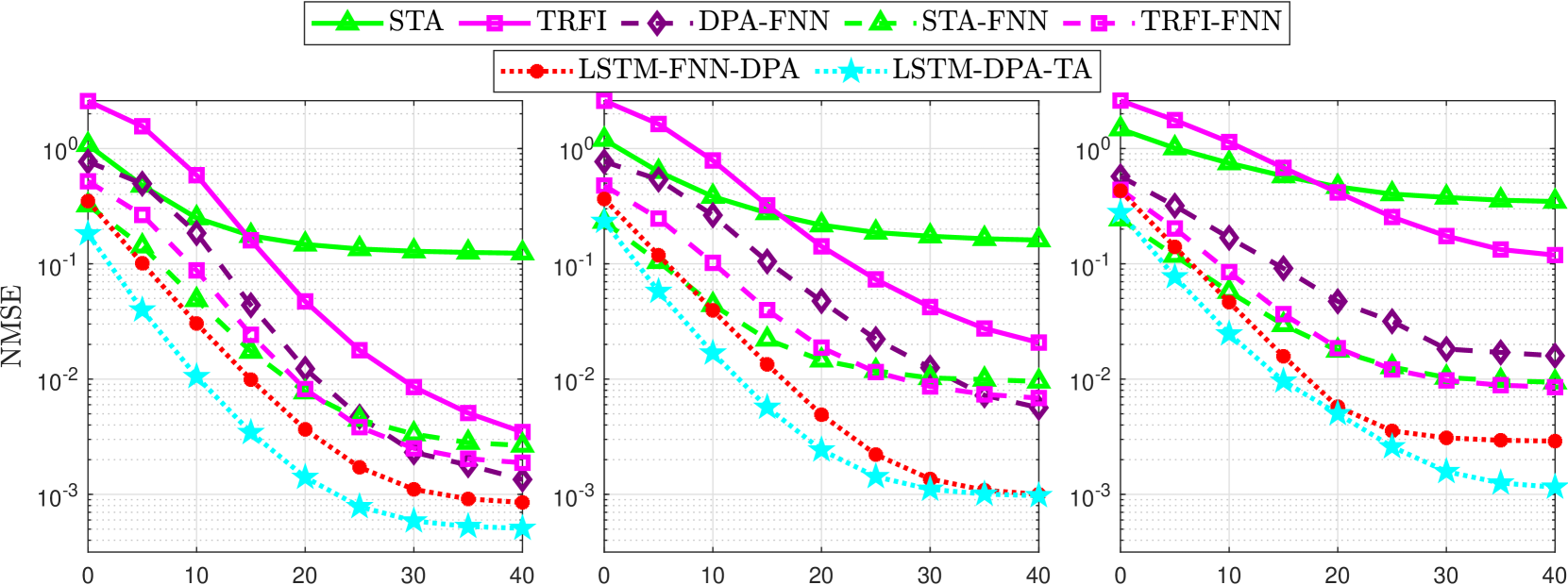
Figure 9: NMSE for $I=100$, mobility from left to right: low ($v=45\leavevmode\nobreak\ \text{Kmph},f_{d}=250$ Hz), high ($v=100\leavevmode\nobreak\ \text{Kmph},f_{d}=500$ Hz), very high ($v=200\leavevmode\nobreak\ \text{Kmph},f_{d}=1000$ Hz).

For QPSK modulation order, we can notice from Figure 8, and Figure 9 that conventional SBS estimators witness a considerable performance degradation in different mobility scenarios primarily due to the enlarged DPA demapping error, particularly under very high mobility. Nevertheless, employing DL techniques in the channel estimation process results in a significant improvement in overall performance. To begin with, the FNN-based estimators, where FNN is employed as a post-processing unit after conventional estimators, are discussed. As observed, FNN can implicitly learn the channel correlations apart from preventing a high demapping error arising from conventional DPA-based estimation, while STA-FNN and TRFI-FNN outperform conventional STA and TRFI estimators by at least $15$ dB gain in terms of SNR for BER $=10^{-3}$. Meanwhile, STA-FNN estimator outperforms DPA-FNN estimator by around $5$ dB gain in terms of SNR for BER $=10^{-3}$. However, STA-FNN suffers from error floor beginning from SNR $=20$ dB, particularly in very high mobility scenarios. This is attributed to the fact that conventional STA estimation outperforms DPA in low SNR region due to the frequency and time averaging operations that can alleviate the impact of noise and demapping error in low SNR regions. On the other hand, the averaging operations are not useful in high SNR regions since the impact of noise is low, and the STA averaging coefficients are fixed. Therefore, TRFI-FNN is used to improve the performance at high SNRs to compensate for the STA-FNN performance degradation in high SNR region. Importantly, STA-FNN and TRFI-FNN can be employed in an adaptive manner where STA-FNN and TRFI-FNN are used in low and high SNR regions, respectively.

For the LSTM-based estimators, employing LSTM as a prepossessing unit rather than a simple FNN in the channel estimation has shown to bring about a significant improvement in the overall performance. This is because LSTM is capable of efficiently learning the time correlations of the channel by taking the advantage of the previous output apart from the current input in order to estimate the current output. LSTM-FNN-DPA estimator [53] outperforms STA-FNN and TRFI-FNN estimators by approximately $4$ dB gain in terms of SNR for BER $=10^{-3}$. However, this estimator is not impervious to high computational complexity, as discussed in the next section, due to the utilization of two DL networks, i.e, LSTM followed by FNN. On the other hand, the LSTM-DPA-TA estimators performance gain in various scenarios can be explained by employing the TA processing, which significantly alleviates the noise impact aside from the strong ability of the LSTM in learning the channel time correlations compared with a simple FNN architecture. The LSTM-DPA-TA estimator outperforms the LSTM-FNN-DPA estimator by around $4$ dB gain in terms of SNR for BER $=10^{-4}$. When adopting high modulation order (16QAM), the LSTM-DPA-TA estimator outperforms the other estimators by at least $7$ dB and $3$ dB gains in terms of SNR for BER $=10^{-3}$ in high as well as very high mobility scenarios, respectively, as illustrated in Figure LABEL:BER_16QAM_DL_SBS.

VI-B2 Mobility

The degraded performance with the increased mobility of all the studied schemes can be observed from Figure 8. However, the time diversity gain increases when there is an increase in the Doppler spread, as evidenced by comparing the case of the DL-based estimators in high mobility $(f_{d}=500)$ and very high mobility ($f_{d}=1000$). This behavior can be explained by the ability of DL networks to reduce the estimation error stemming from the AWGN noise and the DPA demapping error. By contrast, the net gain from the time diversity is influenced by the AWGN noise and DPA demapping error, as is the case in conventional SBS estimators. The performance degradation is attributed as the mobility increases since the impact of the AWGN noise and DPA demapping error is much more dominant than the time diversity gain. This observation is also valid for high modulation orders such as 16QAM, as evidenced in Figure LABEL:BER_16QAM_DL_SBS.

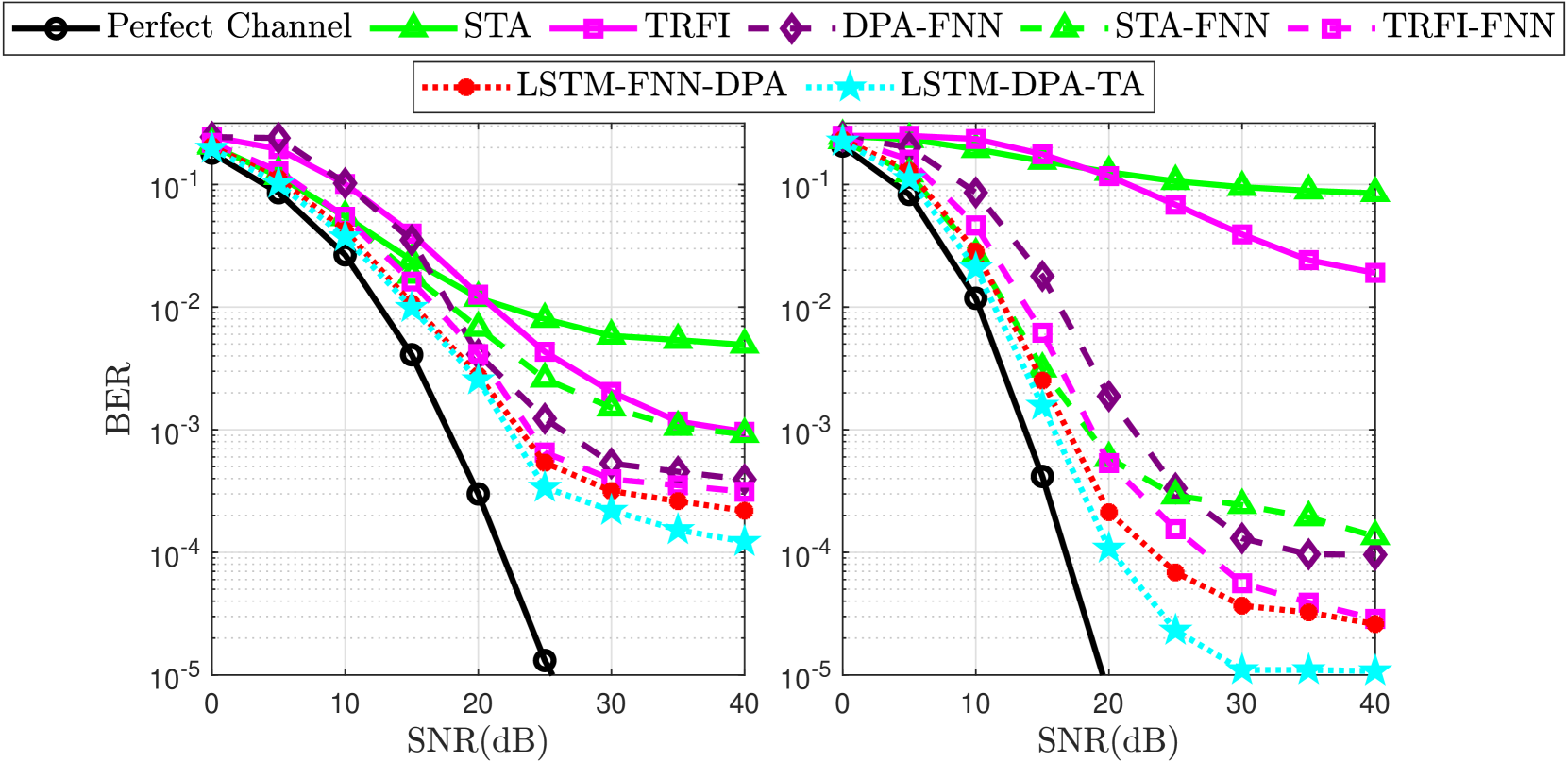
Figure 10: BER for QPSK, very high mobility ($v=200\leavevmode\nobreak\ \text{Kmph},f_{d}=1000$ Hz) from left to right: $I=10$, $I=100$.

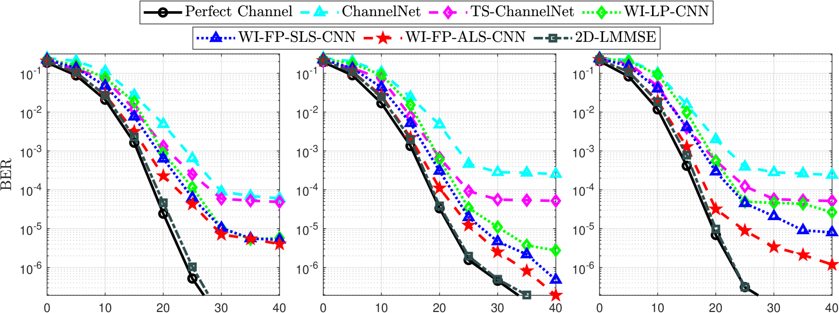
(a)

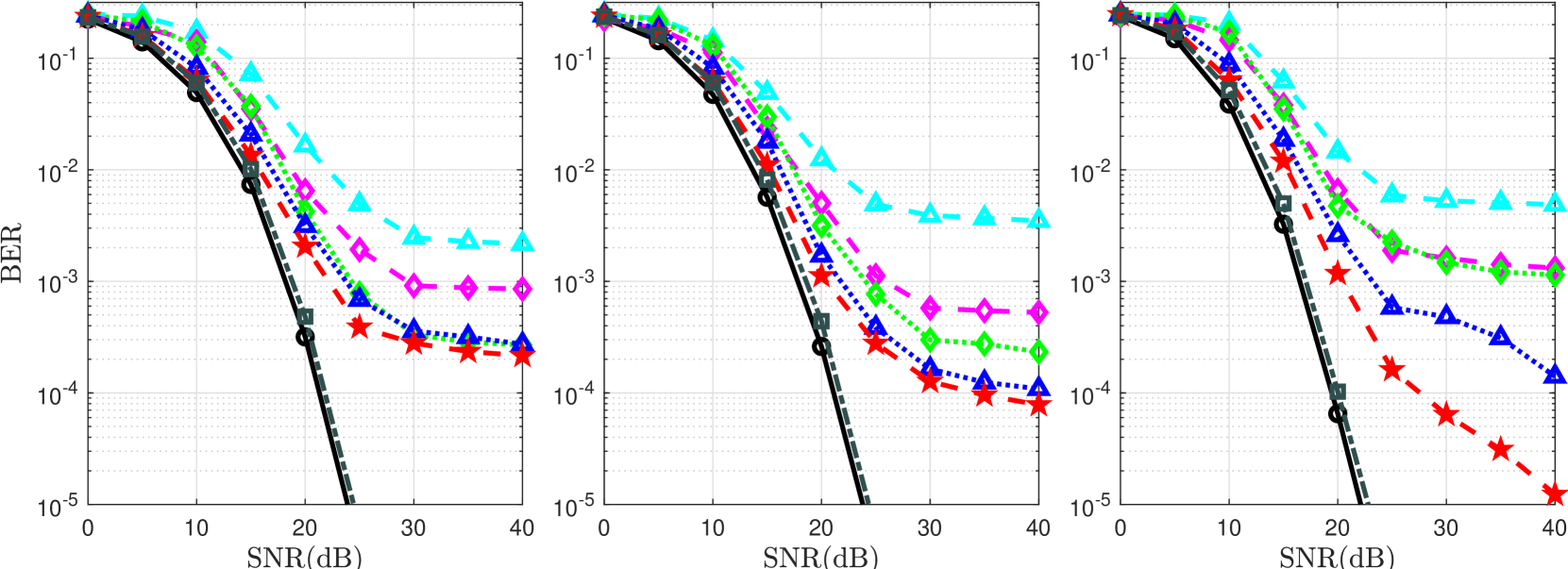
(b)

Figure 11: BER for $I=100$, mobility from left to right: low ($v=45\leavevmode\nobreak\ \text{Kmph},f_{d}=250$ Hz), high ($v=100\leavevmode\nobreak\ \text{Kmph},f_{d}=500$ Hz), very high ($v=200\leavevmode\nobreak\ \text{Kmph},f_{d}=1000$ Hz). The CNN refers to SR-CNN and DN-CNN in low and high/very high) mobility scenarios, respectively.

VI-B3 Frame Length

The impact of frame length is illustrated in Figure 10. As can be seen, the performance of the conventional estimators strongly depends on the frame length, given that employing short frame $I=10$ results in a negligible accumulated DPA demapping error. By contrast, the DL-based estimators are found to be more robust against the changes in the employed frame length. However, in the case of a long frame ($I=100$), the performance gain of the DL-based estimators is significantly remarkable. This behavior is mainly attributed to the time diversity negligible gain when short frame is employed and vice versa.

To conclude, it can be surmised that increasing the frame length increases the time diversity gain. Additionally, the codeword becomes longer with a longer frame. Therefore, the time diversity is capable of compensating for Doppler error, particularly in very high mobility scenario as illustrated in Figure 10

VI-B4 DL Architecture

The DPA-FNN estimator integrates three hidden layer FNN in additon to the conventional DPA estimation with $40-20-40$ neurons. However, as can be observed in Figure 8, correcting the estimation error of the DPA estimation is insufficient even after the inclusion of more neurons in the FNN hidden layers, because it merely corrects the demapping error, neglecting the received symbols’requency and time correlation. Meanwhile, the STA-FNN and TRFI-FNN estimators have better optimized three hidden layers FNN architecture where $15-15-15$ neurons are used. Consequently, the overall computational complexity is considerably lowered when compared to the DPA-FNN, while attaining performance superiority. This is due to the fact that STA considers frequency as well a time correlation between the received OFDM symbols, while the conventional TRFI estimator employs frequency-domain cubic interpolation to make further improvements in the DPA estimation.

Therefore, it can be concluded that the pre-estimation should be good enough in order for the FNN processing to be more useful. Put differently, with an increased accuracy of the pre-estimation, low-complexity FNN architecture can be taken advantage of while recording a significant performance gain. On the contrary, if the pre-estimation is poor, employing FNN processing with high-complexity architecture results in a limited performance gain while increasing the overall computational complexity. As is the case with LSTM-based estimators, employing the TA processing in the LSTM-DPA-TA estimator to ameliorate the AWGN noise impact results in a less complex architecture in comparison to the LSTM-FNN-DPA estimator, where two DL networks are employed.

VI-C DL-Based FBF estimation Scheme

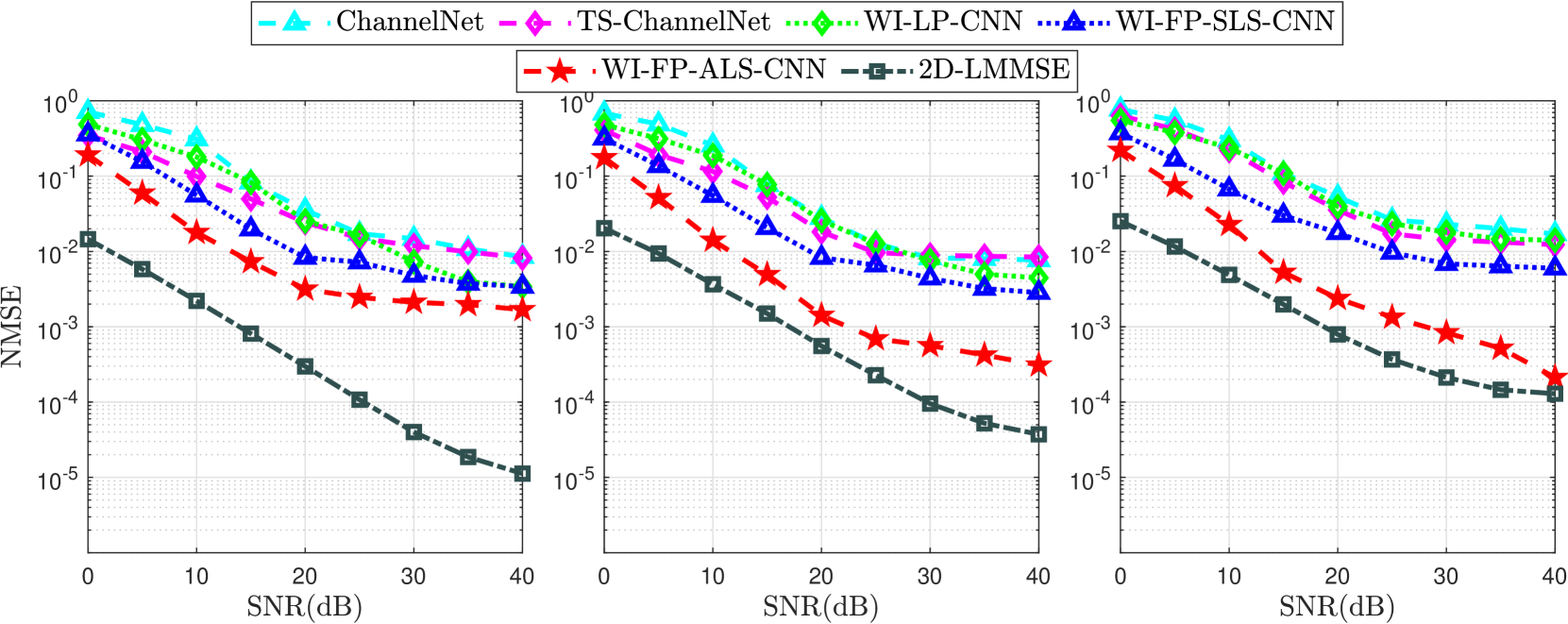
Figure 12: NMSE for $I=100$, mobility from left to right: low ($v=45\leavevmode\nobreak\ \text{Kmph},f_{d}=250$ Hz), high ($v=100\leavevmode\nobreak\ \text{Kmph},f_{d}=500$ Hz), very high ($v=200\leavevmode\nobreak\ \text{Kmph},f_{d}=1000$ Hz).The CNN refers to SR-CNN and DN-CNN in low and high/very high) mobility scenarios, respectively.

VI-C1 Modulation Order

Figure 11 illustrates the BER performance of the studied DL-Based FBF estimators employing QPSK and 16QAM modulation orders. The 2D LMMSE uses the channel and noise statistics in the estimation, thus leading to comparable performance in terms of the ideal case. However, the 2D-LMMSE is ridden with high computational complexity. Moreover, the significant BER performance superiority of the WI-CNN estimators can be observed where FP-ALS-CNN outperforms the ChannelNet as well as TS-ChannelNet estimators by at least $6$ dB and $3$ dB gain in terms of SNR for a BER = $10^{-3}$. Importantly, ChannelNet and TS-ChannelNet estimators suffer from a considerable performance degradation that is dominant in very high mobility scenarios. This is because their performance accounts for the predefined fixed parameters in the applied interpolation scheme, where it is important to update the RBF interpolation function and the ADD-TT frequency and time averaging parameters in real-time. Furthermore, the ADD-TT interpolation employs only the previous and the current pilot subcarriers for the channel estimation at each received OFDM symbol. By contrast, there are no fixed parameters in the WI-CNN estimators. The time correlation between the previous and the future pilot symbols is considered in the WI interpolation matrix (51), whereas the estimated channel is considered in the overall estimation at all channel taps. These aspects lead to the superior performance of WI-CNN estimators performance, where a significant robustness is shown against high mobility with varied performance gain according to the employed pilot allocation scheme, i.e FP or LP. In addition, WI-CNN estimators employ optimized SR-CNN and DN-CNN in accordance with the mobility condition, wherein SR-CNN is utilized in low mobility scenarios, whereas, DN-CNN is employed in high and very high mobility scenarios.

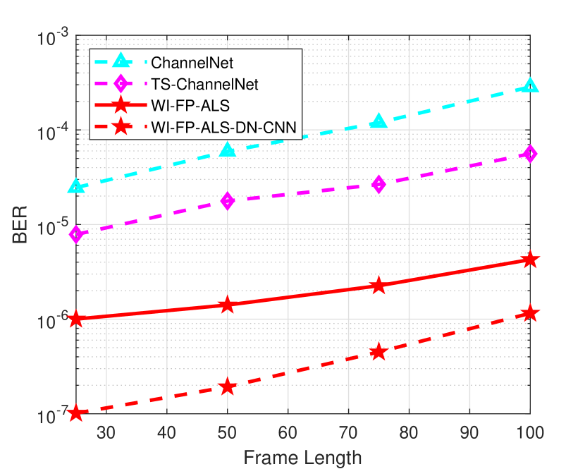
Figure 13: BER performance of VTV-SDWW high mobility vehicular channel model employing QPSK modulation and different frame lengths.

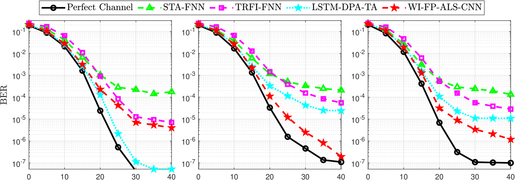
(a)

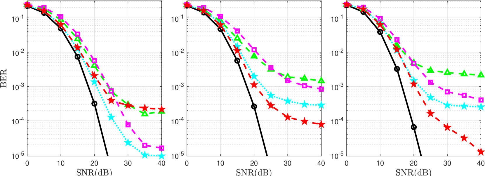
(b)

Figure 14: BER performance employing three scenarios: (i) first column - low mobility ($v=45\leavevmode\nobreak\ \text{Kmph},f_{d}=250$ Hz) (ii) second column - high mobility ($v=100\leavevmode\nobreak\ \text{Kmph},f_{d}=500$ Hz) (iii) third column - very high mobility ($v=200\leavevmode\nobreak\ \text{Kmph},f_{d}=1000$ Hz). The CNN refers to SR-CNN and DN-CNN in low and high/very high) mobility scenarios, respectively.

VI-C2 Mobility

A degradation is observed in the overall performance of ChannelNet and TS-ChannelNet estimators as the mobility increases, while the WI-CNN estimators reveal a robustness against high mobility, as illustrated in Figure 11. This is primarily attributed to the accuracy of the WI interpolation, coupled with optimized SR-CNN and DN-CNN. Although CNN processing is implemented in the ChannelNet and TS-ChannelNet, this post CNN processing is unable to perform well due to the high estimation error of the 2D RBF and ADD-TT interpolation techniques in the initial estimation. Therefore, it can be concluded that employing robust initial estimation as the WI interpolation schemes allows the CNN to better learn the channel correlation with lower complexity, thereby enhancing the channel estimation.

VI-C3 Frame Length

Figure 13 illustrates the BER performance of high mobility vehicular scenario employing QPSK modulation and different frame lengths. As can be clearly observed, the WI-FP-ALS estimator outperforms ChannelNet and TS-ChannelNet for different frame lengths without any post CNN processing. This is because of the long codeword that shows the robustness of the WI-FP-ALS estimator, unlike the 2D RBF and ADD-TT interpolation techniques that suffer from a significant estimation error even when considering a short frame. Moreover, employing the optimized DN-CNN after the WI-FP-ALS estimator significantly enhances the BER performance.

However, although CNN processing is applied in the ChannelNet and TS-ChannelNet, this post CNN processing is unable to perform well. This is attributed to the high estimation error of the 2D RBF and ADD-TT interpolation techniques in the initial estimation. Thus, we can conclude that employing robust initial estimation as the WI interpolation schemes enable the CNN to better learn the channel correlation with lower complexity, thereby enhancing the channel estimation, as shown in Figure 12.

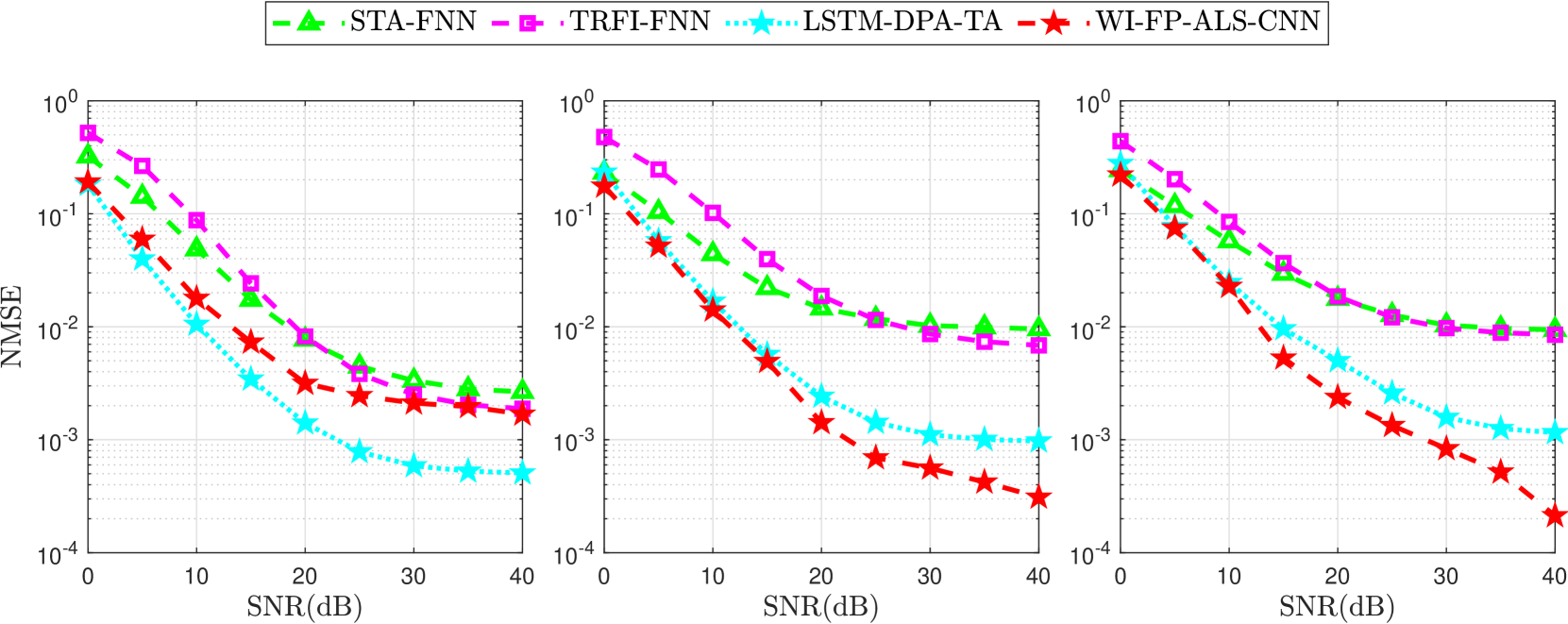
Figure 15: NMSE performance employing three scenarios: (i) first column - low mobility ($v=45\leavevmode\nobreak\ \text{Kmph},f_{d}=250$ Hz) (ii) second column - high mobility ($v=100\leavevmode\nobreak\ \text{Kmph},f_{d}=500$ Hz) (iii) third column - very high mobility ($v=200\leavevmode\nobreak\ \text{Kmph},f_{d}=1000$ Hz). The CNN refers to SR-CNN and DN-CNN in low and high/very high) mobility scenarios, respectively.

VI-D CNN Architecture

The ChannelNet estimator employs SR-CNN and DN-CNN following the 2D RBF interpolation. The employed SR-CNN comprises three convolutional layers with $(v_{1}=9;f_{1}=64),(v_{2}=1,f_{2}=32)$ and $(v_{3}=5,f_{3}=1)$, respectively. Moreover, the DN-CNN depth is $D=18$ with $3\times 3\times 32$ kernels in each layer. Meanwhile, SR-ConvLSTM network comprises three ConvLSTM layers of $(v_{1}=9;f_{1}=64),(v_{2}=1,f_{2}=32)$ and $(v_{3}=5,f_{3}=1)$, respectively, and is integrated after the ADD-TT interpolation in the TS-ChannelNet estimator. The SR-ConvLSTM network combines both the CNN and the LSTM networks [51], thus increasing the overall computational complexity, as shall be discussed later. By contrast, the employed optimized SR-CNN and DN-CNN significantly reduces the complexity due to the WI estimators’ accuracy. Put succinctly, the complexity of the employed CNN decreases as the accuracy of the pre-estimation increases, because low-complexity architectures can be utilized and vice versa.

VI-E DL-Based SBS vs. DL-Based FBF estimation Scheme

This section further examines the performance assessment of the studied estimators, where only the best DL-based SBS and FBF estimators are compared. Figures 14 and 15 illustrate the BER and NMSE performance of the investigated DL-based estimators in low, high, and very high mobility scenarios, employing QPSK and 16QAM modulation orders.

In low-mobility scenario, the LSTM-DPA-TA SBS estimator outperforms the WI-FP-ALS-SR-CNN FBF estimator. This can be explained by the ability of LSTM to better learn the channel time correlation than the SR-CNN, since Doppler error is somehow negligible in low mobility scenario. However, in high and very high mobility scenarios, WI-FP-ALS-DN-CNN shows a significantly improved performance, outperforming the LSTM-DPA-TA SBS estimator by $3$ dB gain in terms of SNR for a BER = $10^{-4}$. In high mobility scenarios, where the Doppler error impact is high, LSTM suffers from some performance degradation as learning the time correlation between successive samples is not achievable in the low mobility scenario case. Meanwhile, DN-CNN network can significantly alleviate the impact of noise and Doppler error, where it records at least $5$ dB gain in terms of SNR for a BER = $10^{-4}$. To conclude, it can be inferred that employing LSTM network rather than FNN and DN-CNN networks leads to improved performance in low-mobility scenarios. In By contrast, DN-CNN is more useful in high as well as very high mobility scenarios because DN-CNN uses the entire pilot subcarriers within the received frame. To summarize, the time correlation between successive received OFDM symbols decreases as the mobility increases. Therefore, the performance of LSTM suffers from performance degradation when compared with CNN. On the other hand, the CNN-based estimators become more useful than the LSTM-based estimators in high mobility scenarios.

Finally, it is observes that DL-based FBF estimators suffer from high buffering time at the receiver, because it is necessary to receive the full frame before the channel estimation begins leading to high latency. However, this buffering time is lowered in the WI-CNN estimators after dividing the received frame into sub frames so that the channel estimation process commences prior to the full frame reception. Moreover, the WI-CNN estimators also help increase the transmission data rate as fewer pilots are inserted into the transmitted frame.

VII Complexity Analysis

This section provides a detailed computational complexity analysis of the studied DL-based SBS and FBF estimators. The computational complexity analysis is performed in accordance with the number of real-valued arithmetic operations, multiplication/division and summation/subtraction necessary to estimate the channel for one received OFDM frame. Each complex-valued division requires $6$ real-valued multiplications, $2$ divisions, $2$ summations, and $1$ subtraction. In addition, each complex-valued multiplication is performed by $4$ real-valued multiplications and $3$ summations.

Figure 16: Computational complexity comparison of the studied DL-based SBS estimators.

Table VI: Detailed computation complexity of the studied DL-based SBS estimators.

Estimator Mul./Div. Sum./Sub. FNN($J_{2}$-$J_{3}$-$J_{4}$) $2K_{\text{on}}J_{2}$ + $J_{2}J_{3}$ + $J_{3}J_{4}$ + $2K_{\text{on}}J_{4}$ $2K_{\text{on}}J_{2}$ + $J_{2}J_{3}$ + $J_{3}J_{4}$ +$2K_{\text{on}}J_{4}$ LSTM ($P$) $P^{2}+3P+PK_{in}$ $4P+K_{in}-2$ Overall channel estimation STA-FNN $82K_{\text{on}}+2K_{d}+450$ $70K_{\text{on}}+10K_{d}+450$ TRFI-FNN $94K_{\text{on}}+26K_{\text{int}}+450$ $74K_{\text{on}}+30K_{\text{int}}+450$ DPA-FNN $178K_{\text{on}}+1600$ $168K_{\text{on}}+1600$ LSTM-FNN-DPA $512K_{\text{in}}+98K_{d}+71040$ $4K_{\text{in}}+88K_{d}+6776$ LSTM-DPA-TA($64$) $514K_{on}+18K_{d}+16576$ $10K_{on}+8K_{d}+824$ LSTM-DPA-TA($128$) $1026K_{on}+18K_{d}+65920$ $10K_{on}+8K_{d}+1656$

VII-A DL-Based SBS Estimators

The DPA estimation implemented in the DL-based SBS estimators as an initial step needs two equalization steps (23), and (25). Each equalization step comprises $K_{\text{on}}$ complex-valued divisions. Moreover, it needs the LS estimated channel at the preamble computed by $2K_{\text{on}}$ summation and $2K_{\text{on}}$ divisions. Hence, the overall computational complexity of the DPA estimation is $16K_{\text{on}}$ multiplications/divisions and $6K_{\text{on}}$ summations/subtractions.

The STA estimator applies frequency as well as time-domain averaging in addition to DPA. The frequency-domain averaging (26) coefficient is fixed ($\beta=2$). Thus, each subcarrier requires $5$ complex-valued summations multiplied by a real-valued weight, which, in turn, are equivalent to $10$ real-valued summations, and $2$ real-valued multiplications. Consequently, the STA frequency-domain averaging step requires $10K_{d}$ real-valued summations, and $2K_{d}$ real-valued multiplications. The STA time-domain averaging step (27) requires $4K_{\text{on}}$ real-valued divisions, and $2K_{\text{on}}$ real-valued summations. For this reason, the accumulated overall computational complexity of STA estimator is $22K_{\text{on}}+2K_{\text{d}}$ multiplications/divisions and $10K_{\text{on}}+10K_{\text{d}}$ summations/subtractions.

The TRFI estimator implements another two equalization steps after the DPA estimation (28). Thereafter, it applies cubic interpolation as the last step. Based on the analysis performed in [28], the computational complexity of TRFI is $34K_{\text{on}}+26K_{\text{int}}$ multiplications/divisions and $14K_{\text{on}}+30K_{\text{int}}$ summations/subtractions, where $K_{\text{int}}$ represents the number of unreliable subcarriers in each received OFDM symbol.

VII-A1 FNN-based Estimators

For the FNN-based estimators, the DPA-FNN architecture [27] consists of three hidden layers with $J_{1}=J_{5}=2K_{\text{on}}$, $J_{2}=J_{4}=40$, and $J_{3}=20$ neurons, respectively. Therefore, the DPA-FNN requires $4K_{\text{on}}J_{2}+2J_{2}J_{3}$ multiplications, and $2K_{\text{on}}+2J_{2}+J_{3}$ summations. The computational complexity of LS and the DPA estimation are accumulated for DPA-FNN computational complexity resulting in total of $178K_{\text{on}}+1600$ multiplications and $168K_{\text{on}}+1600$ summations/subtractions.

$$CC_{\text{FNN}}=2\sum_{l=0}^{L+1}{N}_{l-1}{N}_{l},\leavevmode\nobreak\ \mbox{where }{N}_{0}={N}_{L+1}=2K_{\text{on}}.$$ (54)

The STA-FNN and TRFI-FNN estimators employ a three-hidden layer FNN architecture consisting of $15$ neurons each. This FNN architecture requires $4K_{\text{on}}J_{2}+2J_{2}^{2}$, and $2K_{\text{on}}+3J_{2}$ summations. This architecture is less complex when compared with the DPA-FNN one. Thus, the STA-FNN overall computational complexity is $82K_{\text{on}}+2K_{d}+450$ multiplications, and $70K_{\text{on}}+10K_{d}+450$ summations/subtractions. Furthermore, the TRFI-FNN needs $94K_{\text{on}}+26K_{\text{int}}+450$ multiplications, and $74K_{\text{on}}+30K_{\text{int}}+450$ summations/subtractions. The TRFI-FNN estimator reduces the number of multiplications as well as summations by $48\%$ and $56\%$, respectively, when compared with DPA-FNN, while its computational complexity is similar to that of STA-FNN.

VII-A2 LSTM-Based Estimators

The computational complexity of the LSTM unit can be calculated with respect to the number of operations performed by its four gates. Each gate applies $P^{2}+PK_{in}$ real-valued multiplications and $3P+K_{in}-2$ summations apart from $3P$ multiplications, and $P$ summations required by (19), and (21). As a result, the overall computational complexity for the LSTM becomes

$$CC_{\text{LSTM}}=4(P^{2}+PK_{\text{in}}+3P+K_{\text{in}}-2)+4P.$$ (55)

Notably, FNN-based estimators need less computation than LSTM, thus achieving lower complexity.

Figure 17: Computational complexity comparison of the studied DL-based FBF estimators.

The LSTM-FNN-DPA estimator employs one LSTM unit with $P=128$ and $K_{in}=112$, followed by one hidden layer FNN network with $N_{1}=40$ neurons. In addition, the LSTM-FNN-DPA estimator implements the DPA estimation that requires $18K_{d}$ real-valued multiplication/division and $8K_{d}$ summation/subtraction. Thus, the overall computational complexity of the LSTM-FNN-DPA estimator is $512K_{\text{in}}+98K_{d}+71040$ multiplication/division and $4K_{\text{in}}+88K_{d}+6776$ summation/subtraction.

The LSTM-DPA-TA utilizes one LSTM unit with $P=128$ as LSTM-FNN-DPA estimator. It also uses $K_{in}=2K_{on}$, and applies TA as a noise alleviation technique to the $\hat{\bar{\bm{h}}}_{\text{LSTM-DPA}_{i,d}}$ estimated channel, that requires only $2K_{on}$ real-valued multiplication/division and $2K_{on}$ summation/subtraction. Hence, the LSTM-DPA-TA estimator requires $4P^{2}+P(8K_{on}+3)+18K_{d}+2K_{on}$ real-valued multiplication/division and $13P+10K_{on}+8K_{d}-8$ summation/subtraction. As per this analysis, the LSTM-DPA-TA estimator achieves less computational complexity in comparison to the LSTM-FNN-DPA estimator. It records $9.73\%$ and $77.63\%$ computational complexity decline in the required real-valued multiplication/division and summation/subtraction, respectively. Importantly, replacing the FNN network by the TA to achieve noise alleviation is the primary factor in reducing the overall computational complexity. Moreover, the LSTM-DPA-TA estimator outperforms the LSTM-FNN-DPA estimator while recording lower computational complexity. As a matter of fact, employing the LSTM-DPA-TA LSTM-based estimators as opposed to the FNN-based estimators results in $89.10\%$ and $62.18\%$ increase in the necessary multiplication/division and summation/subtraction, respectively. Nevertheless, it is possible to achieve a significant performance gain. Table VI and Figure 16 reveal a detailed summary of the computational complexities for the various examined DL-based SBS estimators.

VII-B DL-Based FBF Estimators

VII-B1 ChannelNet estimator

The ChannelNet estimator utilizes the RBF interpolation followed by SR-CNN and DN-CNN networks. Therefore, the overall computational complexity of the ChannelNet estimator can be expressed as follows

$$\text{CC}_{{\text{ChannelNet}}}=\text{CC}_{{\text{RBF}}}+\text{CC}_{\text{SR-CNN}}+\text{CC}_{\text{DN-CNN}}.$$ (56)

The calculation of $\hat{\tilde{\bm{H}}}_{\text{LS}}$ requires $2K_{p}I$ divisions. The computation of $\bm{w}_{\text{RBF}}$ requires $4K^{2}_{p}I^{2}$ multiplications/divisions and $5K^{2}_{p}I^{2}-2K_{p}I$ summations/subtractions. Meanwhile, $\hat{\tilde{\bm{H}}}_{\text{RBF}}$ requires $K_{d}I(K^{2}_{p}I^{2}+3K_{p}I)$ multiplications/divisions and $5K_{d}K_{p}I^{2}$ subtractions/summations. Thus, the total computational complexity of the RBF interpolation can be expressed by $K^{2}_{p}I^{2}(4+K_{d}I)+K_{p}I(2+3K_{d}I)$ multiplications/divisions and $K_{p}I(5K_{p}I+5K_{d}I-2)$ summations/subtractions. Subsequently, the ChannelNet estimator applies SR-CNN followed by DN-CNN in addition to the RBF interpolation. $\text{CC}_{\text{SR-CNN}}$ and $\text{CC}_{\text{DN-CNN}}$ can be computed as follows

$$\begin{split}\text{CC}_{\text{SR-CNN}}&=\sum_{l=1}^{\mathcal{L}}h_{l}w_{l}d_{l}v_{l}^{2}f_{l}+h_{l}w_{l}d_{l}f_{l}\\ &=\sum_{l=1}^{\mathcal{L}}h_{l}w_{l}d_{l}f_{l}(v_{l}^{2}+1).\end{split}$$ (57)

$$\text{CC}_{\text{DN-CNN}}=\sum_{l=1}^{\mathcal{L}}h_{l}w_{l}d_{l}f_{l}(v_{l}^{2}+1)+\sum_{j=1}^{D}4h_{j}w_{j}d_{j}.$$ (58)

$\mathcal{L}$ signifies the number of employed CNN layers. It can be noted that the second term in $\text{CC}_{\text{DN-CNN}}$ signifies the number of operations required by the batch normalization employed in the DN-CNN network. Thus, the SR-CNN employed in the ChannelNet estimator needs $16064K_{\text{on}}I$ multiplications/divisions as well as $4288K_{\text{on}}I$ summations/subtractions, while the ChannelNet DN-CNN computations require $334080K_{\text{on}}I$ multiplications/divisions and $38144K_{\text{on}}I$ summations/subtractions.

Table VII: Detailed computation complexity of the studied CNN-based FBF estimators.

Scheme Interpolation CNN Mul./Div. Sum./Sub. Mul./Div. Sum./Sub. ChannelNet $K^{2}_{p}I^{2}(4+K_{d}I)$ + $K_{p}I(2+3K_{d}I)$ $K_{p}I(5K_{p}I$ + $5K_{d}I-2)$ $350144K_{\text{on}}I$ $42432K_{\text{on}}I$ TS-ChannelNet $24K_{\text{on}}I+4LK_{\text{on}}I$ $18K_{\text{on}}I$ + $5K_{\text{on}}IL$ $226880K_{\text{on}}I$ $81472K_{\text{on}}I$ FP-SLS-SR-CNN $2K_{\text{on}}P+2K_{\text{on}}$ + $4K_{\text{on}}I_{d}$ $2K_{\text{on}}$ + $2K_{\text{on}}I_{d}$ $7008K_{\text{on}}I_{d}$ $1120K_{\text{on}}I_{d}$ FP-ALS-SR-CNN $4K^{2}_{\text{on}}P+2K_{\text{on}}P$ + $2K_{\text{on}}+4K_{\text{on}}I_{d}$ $5K^{2}_{\text{on}}P$ + $2K_{\text{on}}I_{d}$ LP-SR-CNN $2LP+4K_{\text{on}}LP$ + $2K_{\text{on}}+4K_{\text{on}}I_{d}$ $5K_{\text{on}}LP$ + $2K_{\text{on}}I_{d}$ FP-SLS-DN-CNN $2K_{\text{on}}P+2K_{\text{on}}$ + $4K_{\text{on}}I_{d}$ $2K_{\text{on}}$ + $2K_{\text{on}}I_{d}$ $84096K_{\text{on}}I_{d}$ $9856K_{\text{on}}I_{d}$ FP-ALS-DN-CNN $4K^{2}_{\text{on}}P+2K_{\text{on}}P$ + $2K_{\text{on}}+4K_{\text{on}}I_{d}$ $5K^{2}_{\text{on}}P$ + $2K_{\text{on}}I_{d}$ LP-DN-CNN $2LP+4K_{\text{on}}LP+2K_{\text{on}}$ + $4K_{\text{on}}I_{d}$ $5K_{\text{on}}LP$ + $2K_{\text{on}}I_{d}$

VII-B2 TS-ChannelNet estimator

The TS-ChannelNet estimator applies the ADD-TT interpolation followed by the SR-ConvLSTM network. Hence, the overall computational complexity of the TS-ChannelNet estimator can be expressed in the following manner:

$$\text{CC}_{{\text{TS-ChannelNet}}}=\text{CC}_{{\text{ADD-TT}}}+\text{CC}_{\text{SR-ConvLSTM}}.$$ (59)

The ADD-TT interpolation first applies the DPA estimation requiring $18K_{\text{on}}$ multiplications/divisions and $8K_{\text{on}}$ summations/subtractions. The time-domain truncation operation applied in (43) requires $4LK_{\text{on}}$ multiplications as well as $5K_{\text{on}}L-2K_{\text{on}}$ summations. In the ADD-TT interpolation, the frequency-domain averaging (44) requires $10K_{\text{on}}$ summations and $2K_{\text{on}}$ multiplications. Furthermore, the time-domain averaging step (45) requires $4K_{\text{on}}$ real valued divisions, and $2K_{\text{on}}$ real valued summations. Thus, the overall computational complexity of the ADD-TT interpolation for the whole received OFDM frame requires $24K_{\text{on}}I+4LK_{\text{on}}I$ real-valued multiplications/divisions, and $18K_{\text{on}}I+5K_{\text{on}}IL$ summations/subtractions. The total computational complexity is expressed with respect to the overall operations implemented in the input, forget, and output gates of the SR-ConvLSTM network, such that

$$\text{CC}_{\text{ConvLSTM}}=\sum_{l=1}^{\mathcal{L}}h_{l}w_{l}d_{l}f_{l}(8v_{l}^{2}+30).$$ (60)

Based on (60), the SR-ConvLSTM network employed in the TS-ChannelNet estimator requires $226880K_{\text{on}}I$ multiplications/divisions as well as $81472K_{\text{on}}I$ summations/subtractions. TS-ChannelNet estimator is less complicated than the ChannelNet estimator, because it employs only one CNN in addition to the ADD-TT interpolation, unlike the ChannelNet estimator where both SR-CNN and DN-CNN are employed.

VII-B3 WI-CNN estimators

The WI-CNN estimators computational complexity primarily depends on the selected frame structure, the pilot allocation scheme, as well as the selected optimized CNN. Thus, the overall computational complexity of the WI-CNN estimators can be expressed as follows

$$\text{CC}_{{\text{WI}}}=\text{CC}_{\hat{\tilde{\bm{H}}}_{\text{WI}}}+\text{CC}_{\text{O-CNN}}.$$ (61)

When full pilot symbols are inserted, two options are taken into consideration. The first option is the SLS estimator, which is performed using $2K_{\text{on}}P+2K_{\text{on}}$ divisions, and $2K_{\text{on}}$ summations. The second option entails employing the ALS estimator with $2K_{\text{on}}P+2K_{\text{on}}$ divisions. This is followed by $4K^{2}_{\text{on}}P$ multiplications, and $5K^{2}_{\text{on}}P$ summations. In the instance where $K_{\text{p}}=L$ pilots are inserted with each pilot symbol, the LS estimation requires $2LP+2K_{\text{on}}$ divisions, $4K_{\text{on}}LP$ multiplications, and $5K_{\text{on}}LP$ summations. In a similar manner, for employing only $K_{p}=4$ pilot subcarriers, the WI-CP estimator needs $8P+2K_{\text{on}}$ divisions, $16K_{\text{on}}P$ multiplications, as well as $20K_{\text{on}}P$ summations. Following the selection of the required frame structure and pilot allocation scheme, the WI-CNN estimators apply the weighted interpolation as demonstrated in (50).The channel estimation for each received OFDM frame needs $4K_{\text{on}}I_{d}$ divisions and $2K_{\text{on}}I_{d}$ summations. Finally, the optimized SR-CNN is utilized in low-mobility scenario and needs $7008K_{\text{on}}I_{d}$ multiplications/divisions and $1120K_{\text{on}}I_{d}$ summations/subtractions. For high-mobility scenarios, the optimized DN-CNN is employed, requiring $84096K_{\text{on}}I_{d}$ multiplications/divisions and $9856K_{\text{on}}I_{d}$ summations/subtractions. The WI-FP-ALS records the higher computational complexity among the other WI estimators in all mobility scenarios, due to $\bm{W}_{\text{ALS}}$ calculation in (47), whereas, the WI-FP-SLS estimator refers to the simplest one.

Table VII shows the studied estimators’ overall computational complexity with respect to real valued operations. It is noteworthy that the WI estimators achieve significant computational complexity decrease in comparison to ChannelNet and TS-ChannelNet estimators. Figure 17 depicts the computational complexity of the studied DL-based FBF estimators. The ChannelNet and TS-ChannelNet estimators are $70$ and $39$ times more complex than the FP-ALS-SR-CNN, respectively. In addition, the WI-CNN estimators achieve a minimum of $7027.35$ times less complexity than the 2D LMMSE estimator, with an acceptable BER performance, which makes them a feasible alternative to the 2D LMMSE. It is also observed that FP-ALS-DN-CNN is $12$ times more complex than FP-ALS-SR-CNN since the optimized DN-CNN architecture complexity employed in high and very high scenarios is higher than the optimized SR-CNN architecture, which, in turn, is employed in low mobility scenarios.

VIII Conclusion

This survey sheds light on the recently proposed DL-based SBS and FBF channel estimators in doubly-dispersive environments. First, we have defined the problem of signal propagation in doubly-dispersive channels. Subsequently, a review of different DL architectures employed in the doubly-dispersive channel estimation has been undertaken, followed by a detailed presentation of the studied DL-based estimators. Finally, the studied estimators have been evaluated with respect to NMSE, BER, and computational complexity, clearly demonstrating a significant improvement of employing DL in the channel estimation across different mobility conditions. We have shown that, while the LSTM and CNN based estimators do outperform the FNN based estimator, more computational complexity is necessary where the LSTM-based SBS estimator is $23.6$ times more complex than the FNN-based SBS estimators. Nevertheless, the complexity of the CNN-based FBF estimator exceeds the complexity of LSTM-based SBS estimator by approximately $3450$ times because of the significant difference in terms of required operations between the CNN and LSTM networks. Finally, we have observed that the choice of the channel estimator is primarily related to the applications requirements as well as affordable computational complexity. SBS estimators are more useful when the application is sensitive to latency, whereas FBF estimators can be employed if some latency can be accepted. To summarize, a trade-off between the required performance, computational complexity, and the accepted latency must first be defined to select what is the most suitable channel estimator to be employed.

References

- [1] H. Chang, C.-X. Wang, Y. Liu, J. Huang, J. Sun, W. Zhang, and X. Gao, “A Novel Nonstationary 6G UAV-to-Ground Wireless Channel Model With 3-D Arbitrary Trajectory Changes,” IEEE Internet of Things Journal, vol. 8, no. 12, pp. 9865–9877, 2021.
- [2] L. Wang, B. Ai, K. Guan, D. He, Z. Zhong, L. Tian, and J. Dou, “Stochastic Channel Modeling for High-Speed Railway Viaduct Scenario at 93.2 GHz,” in 12th European Conference on Antennas and Propagation (EuCAP 2018), 2018, pp. 1–4.
- [3] B. Turan and S. Coleri, “Machine Learning Based Channel Modeling for Vehicular Visible Light Communication,” IEEE Transactions on Vehicular Technology, vol. 70, no. 10, pp. 9659–9672, 2021.
- [4] R. Chen, W. Yang, F. Wu, and M. Sun, “Fast Handover for High-Speed Railway via NDN,” in 2018 1st IEEE International Conference on Hot Information-Centric Networking (HotICN), 2018, pp. 167–172.
- [5] S. Wang and Q. Zhang, “A Joint Time-Frequency Domain Frequency Offset Estimation Algorithm for Busrt Communication,” in 2020 IEEE 3rd International Conference on Electronics Technology (ICET), 2020, pp. 1–5.
- [6] T. Ma, X. Jiang, Y. Wang, and F. Li, “A Novel Inter-Carrier Interference Cancellation Scheme in Highly Mobile Environments,” China Communications, vol. 17, no. 12, pp. 194–205, 2020.
- [7] K. Saito, Q. Fan, N. Keerativoranan, and J.-i. Takada, “4.9 GHz Band Outdoor to Indoor Propagation Loss Analysis in High Building Environment Using Unmanned Aerial Vehicle,” in 2019 13th European Conference on Antennas and Propagation (EuCAP), 2019, pp. 1–4.
- [8] R. Bomfin, M. Chafii, A. Nimr, and G. Fettweis, “A Robust Baseband Transceiver Design for Doubly-Dispersive Channels,” IEEE Transactions on Wireless Communications, 2021.
- [9] ——, “A Robust Baseband Transceiver Design for Doubly-Dispersive Channels,” IEEE Transactions on Wireless Communications, vol. 20, no. 8, pp. 4781–4796, 2021.
- [10] R. Bomfin, A. Nimr, M. Chafii, and G. Fettweis, “A Robust and Low-Complexity Walsh-Hadamard Modulation for Doubly-Dispersive Channels,” IEEE Communications Letters, vol. 25, no. 3, pp. 897–901, 2021.
- [11] A. Nimr, M. Chafii, M. Matthe, and G. Fettweis, “Extended GFDM Framework: OTFS and GFDM Comparison,” in 2018 IEEE Global Communications Conference (GLOBECOM), 2018, pp. 1–6.
- [12] M. Chafii, J. Palicot, R. Gribonval, and F. Bader, “Adaptive Wavelet Packet Modulation,” IEEE Transactions on Communications, vol. 66, no. 7, pp. 2947–2957, 2018.
- [13] J. A. Fernandez, K. Borries, L. Cheng, B. V. K. Vijaya Kumar, D. D. Stancil, and F. Bai, “Performance of the 802.11p Physical Layer in Vehicle-to-Vehicle Environments,” IEEE Transactions on Vehicular Technology, vol. 61, no. 1, pp. 3–14, 2012.
- [14] Z. Zhao, X. Cheng, M. Wen, B. Jiao, and C. Wang, “Channel Estimation Schemes for IEEE 802.11p Standard,” IEEE Intelligent Transportation Systems Magazine, vol. 5, no. 4, pp. 38–49, 2013.
- [15] Yoon-Kyeong Kim, Jang-Mi Oh, Yoo-Ho Shin, and Cheol Mun, “Time and Frequency Domain Channel Estimation Scheme for IEEE 802.11p,” in 17th International IEEE Conference on Intelligent Transportation Systems (ITSC), 2014, pp. 1085–1090.
- [16] S. Ehsanfar, M. Chafii, and G. P. Fettweis, “On UW-based Transmission for MIMO Multi-carriers with Spatial Multiplexing,” IEEE Transactions on Wireless Communications, vol. 19, no. 9, pp. 5875–5890, 2020.
- [17] Y. Choi, J. H. Bae, and J. Lee, “Low-Complexity 2D LMMSE Channel Estimation for OFDM Systems,” in 2015 IEEE 82nd Vehicular Technology Conference (VTC2015-Fall), 2015, pp. 1–5.
- [18] T. Wang, C.-K. Wen, H. Wang, F. Gao, T. Jiang, and S. Jin, “Deep Learning for Wireless Physical Layer: Opportunities and Challenges,” 2017.
- [19] T. O’Shea and J. Hoydis, “An Introduction to Deep Learning for the Physical Layer,” IEEE Transactions on Cognitive Communications and Networking, vol. 3, no. 4, pp. 563–575, 2017.
- [20] M. Chafii, F. Bader, and J. Palicot, “Enhancing Coverage in Narrow Band-IoT Using Machine Learning,” in 2018 IEEE Wireless Communications and Networking Conference (WCNC). IEEE, 2018, pp. 1–6.
- [21] Y. Yang, F. Gao, X. Ma, and S. Zhang, “Deep Learning-Based Channel Estimation for Doubly Selective Fading Channels,” IEEE Access, vol. 7, pp. 36 579–36 589, 2019.
- [22] X. Ma, H. Ye, and Y. Li, “Learning Assisted Estimation for Time- Varying Channels,” in 2018 15th International Symposium on Wireless Communication Systems (ISWCS), 2018, pp. 1–5.
- [23] H. Ye, G. Y. Li, and B. Juang, “Power of Deep Learning for Channel Estimation and Signal Detection in OFDM Systems,” IEEE Wireless Communications Letters, vol. 7, no. 1, pp. 114–117, 2018.
- [24] J. Yuan, H. Q. Ngo, and M. Matthaiou, “Machine Learning-Based Channel Prediction in Massive MIMO With Channel Aging,” IEEE Transactions on Wireless Communications, vol. 19, no. 5, pp. 2960–2973, 2020.
- [25] H. Kim, S. Kim, H. Lee, C. Jang, Y. Choi, and J. Choi, “Massive MIMO Channel Prediction: Kalman Filtering Vs. Machine Learning,” IEEE Transactions on Communications, vol. 69, no. 1, pp. 518–528, 2021.
- [26] C. Wu, X. Yi, Y. Zhu, W. Wang, L. You, and X. Gao, “Channel Prediction in High-Mobility Massive MIMO: From Spatio-Temporal Autoregression to Deep Learning,” IEEE Journal on Selected Areas in Communications, vol. 39, no. 7, pp. 1915–1930, 2021.
- [27] S. Han, Y. Oh, and C. Song, “A Deep Learning Based Channel Estimation Scheme for IEEE 802.11p Systems,” in ICC 2019 - 2019 IEEE International Conference on Communications (ICC), 2019, pp. 1–6.
- [28] A. K. Gizzini, M. Chafii, A. Nimr, and G. Fettweis, “Deep Learning Based Channel Estimation Schemes for IEEE 802.11p Standard,” IEEE Access, vol. 8, pp. 113 751–113 765, 2020.
- [29] ——, “Joint TRFI and Deep Learning for Vehicular Channel Estimation,” in 2020 IEEE Globecom Workshops (GC Wkshps, 2020, pp. 1–6.
- [30] M. Soltani, V. Pourahmadi, A. Mirzaei, and H. Sheikhzadeh, “Deep Learning-Based Channel Estimation,” IEEE Communications Letters, vol. 23, no. 4, pp. 652–655, 2019.
- [31] X. Zhu, Z. Sheng, Y. Fang, and D. Guo, “A Deep Learning-Aided Temporal Spectral ChannelNet for IEEE 802.11p-Based Channel Estimation in Vehicular Communications,” EURASIP Journal on Wireless Communications and Networking, vol. 1, no. 94, 2020.
- [32] A. Karim Gizzini, M. Chafii, A. Nimr, R. M. Shubair, and G. Fettweis, “CNN Aided Weighted Interpolation for Channel Estimation in Vehicular Communications,” IEEE Transactions on Vehicular Technology, vol. 70, no. 12, pp. 12 796–12 811, 2021.
- [33] H. A. Le, T. Van Chien, T. H. Nguyen, H. Choo, and V. D. Nguyen, “Machine Learning-Based 5G-and-Beyond Channel Estimation for MIMO-OFDM Communication Systems,” Sensors, vol. 21, no. 14, 2021. [Online]. Available: https://www.mdpi.com/1424-8220/21/14/4861
- [34] F. Tang, B. Mao, N. Kato, and G. Gui, “Comprehensive survey on machine learning in vehicular network: Technology, applications and challenges,” IEEE Communications Surveys Tutorials, vol. 23, no. 3, pp. 2027–2057, 2021.
- [35] A. K. Gizzini, “Dl-based channel estimation in doubly dispersive environments,” in DL-based Channel Estimation in Doubly Dispersive Environments, 2022. [Online]. Available: https://github.com/abdulkarimgizzini/DL-based-Channel-Estimation-in-Doubly-Dispersive-Environments-/
- [36] G. Matz and F. Hlawatsch, “Chapter 1 - fundamentals of time-varying communication channels,” in Wireless Communications Over Rapidly Time-Varying Channels, F. Hlawatsch and G. Matz, Eds. Oxford: Academic Press, 2011, pp. 1–63. [Online]. Available: https://www.sciencedirect.com/science/article/pii/B9780123744838000017
- [37] ——, “Chapter 1 - Fundamentals of Time-Varying Communication Channels,” in Wireless Communications Over Rapidly Time-Varying Channels, 2011, pp. 1–63.
- [38] N. D. Ricklin, “Time Varying Channels : Characterization, Estimation, and Detection,” Ph.D. dissertation, University of California, San Diego, 2010.
- [39] J. Schmidhuber, “Deep Learning in Neural Networks: An Overview,” Neural Networks, vol. 61, p. 85–117, Jan 2015. [Online]. Available: http://dx.doi.org/10.1016/j.neunet.2014.09.003
- [40] S. ichi Amari, “Backpropagation and Stochastic Gradient Descent Method,” Neurocomputing, vol. 5, no. 4, pp. 185 – 196, 1993.
- [41] S. De, A. Mukherjee, and E. Ullah, “Convergence Guarantees for RMSProp and ADAM in Non-Convex Optimization and An Empirical Comparison to Nesterov Acceleration,” 2018.
- [42] S. Ruder, “An Overview of Multi-Task Learning in Deep Neural Networks,” 2017.
- [43] A. K. Gizzini, M. Chafii, S. Ehsanfar, and R. M. Shubair, “Temporal Averaging LSTM-based Channel Estimation Scheme for IEEE 802.11p Standard,” in IEEE Global Communications Conference, Madrid, Spain, Dec. 2021. [Online]. Available: https://hal.archives-ouvertes.fr/hal-03365697
- [44] K. Greff, R. K. Srivastava, J. Koutník, B. R. Steunebrink, and J. Schmidhuber, “LSTM: A Search Space Odyssey,” IEEE Transactions on Neural Networks and Learning Systems, vol. 28, no. 10, pp. 2222–2232, 2017.
- [45] S. Albawi, T. A. Mohammed, and S. Al-Zawi, “Understanding of a Convolutional Neural Network,” in 2017 International Conference on Engineering and Technology (ICET), 2017, pp. 1–6.
- [46] A. K. Gizzini, “Advanced Linear and Deep Learning Based Channel Estimation Techniques in Doubly Dispersive Environments,” Theses, Cergy Paris CY Université, Dec. 2021. [Online]. Available: https://hal.archives-ouvertes.fr/tel-03482053
- [47] M. Sun, Z. Song, X. Jiang, J. Pan, and Y. Pang, “Learning Pooling for Convolutional Neural Network,” Neurocomputing, vol. 224, pp. 96–104, 2017.
- [48] H. Qi, “Derivation of Backpropagation in Convolutional Neural Network (CNN),” in Derivation of Backpropagation in Convolutional Neural Network ( CNN ), 2016.
- [49] C. Dong, C. C. Loy, K. He, and X. Tang, “Image Super-Resolution Using Deep Convolutional Networks,” IEEE Transactions on Pattern Analysis and Machine Intelligence, vol. 38, no. 2, pp. 295–307, 2016.
- [50] K. Zhang, W. Zuo, Y. Chen, D. Meng, and L. Zhang, “Beyond a Gaussian Denoiser: Residual Learning of Deep CNN for Image Denoising,” IEEE Transactions on Image Processing, vol. 26, no. 7, pp. 3142–3155, 2017.
- [51] X. Shi, Z. Chen, H. Wang, D.-Y. Yeung, W. kin Wong, and W. chun Woo, “Convolutional LSTM Network: A Machine Learning Approach for Precipitation Nowcasting,” 2015.
- [52] K. He, X. Zhang, S. Ren, and J. Sun, “Deep Residual Learning for Image Recognition,” in Proceedings of the IEEE Conference on Computer Vision and Pattern Recognition (CVPR), June 2016.
- [53] J. Pan, H. Shan, R. Li, Y. Wu, W. Wua, and T. Q. S. Quek, “Channel Estimation Based on Deep Learning in Vehicle-to-everything Environments,” IEEE Communications Letters, pp. 1–1, 2021.
- [54] A. K. Gizzini, M. Chafii, A. Nimr, and G. Fettweis, “Enhancing Least Square Channel Estimation Using Deep Learning,” in 2020 IEEE 91st Vehicular Technology Conference (VTC2020-Spring), 2020, pp. 1–5.
- [55] F. Pontes, G. Amorim, P. Balestrassi, A. Paiva, and J. Ferreira, “Design of Experiments and Focused Grid Search for Neural Network Parameter Optimization,” Neurocomputing, vol. 186, pp. 22 – 34, 2016.
- [56] C. Chatfield, Time-Series Forecasting. Chapman and Hall/CRC, 2000.
- [57] Y. R. Zheng and C. Xiao, “Channel Estimation for Frequency-Domain Equalization of Single-Carrier Broadband Wireless Communications,” IEEE Transactions on Vehicular Technology, vol. 58, no. 2, pp. 815–823, 2009.
- [58] G. Acosta-Marum and M. A. Ingram, “Six Time and Frequency Selective Empirical Channel Models for Vehicular Wireless LANs,” IEEE Vehicular Technology Magazine, vol. 2, no. 4, pp. 4–11, 2007.
- [59] G. Acosta-Marum, “Measurement, Modeling, and OFDM Synchronization for the Wideband Mobile-to-Mobile Channel,” Ph.D. dissertation, Georgia Inst. Technol., Atlanta, GA, 2007.