Robust space-time finite element error estimates
for parabolic distributed optimal control problems
with energy regularization

Abstract

We consider space-time tracking optimal control problems for linear parabolic initial boundary value problems that are given in the space-time cylinder $Q=\Omega\times(0,T)$, and that are controlled by the right-hand side $z_{\varrho}$ from the Bochner space $L^{2}(0,T;H^{-1}(\Omega))$. So it is natural to replace the usual $L^{2}(Q)$ norm regularization by the energy regularization in the $L^{2}(0,T;H^{-1}(\Omega))$ norm. We derive a priori estimates for the error $\|\widetilde{u}_{\varrho h}-\overline{u}\|_{L^{2}(Q)}$ between the computed state $\widetilde{u}_{\varrho h}$ and the desired state $\overline{u}$ in terms of the regularization parameter $\varrho$ and the space-time finite element mesh-size $h$, and depending on the regularity of the desired state $\overline{u}$. These estimates lead to the optimal choice $\varrho=h^{2}$. The approximate state $\widetilde{u}_{\varrho h}$ is computed by means of a space-time finite element method using piecewise linear and continuous basis functions on completely unstructured simplicial meshes for $Q$. The theoretical results are quantitatively illustrated by a series of numerical examples in two and three space dimensions.

Keywords: Parabolic optimal control problems, energy regularization,
space-time finite element methods, error estimates.

2010 MSC: 49J20, 49M05, 35K20, 65M60, 65M15

1 Introduction

As in [8], we consider the minimization of the space-time tracking cost functional

$${\mathcal{J}}(u_{\varrho},z_{\varrho})=\frac{1}{2}\int_{0}^{T}\int_{\Omega}[u_{\varrho}(x,t)-\overline{u}(x,t)]^{2}\,dx\,dt+\frac{1}{2}\,\varrho\,\|z_{\varrho}\|^{2}_{L^{2}(0,T;H^{-1}(\Omega))}$$ (1.1)

with respect to the state $u_{\varrho}$ and the control $z_{\varrho}$ subject to the model parabolic initial boundary value problem

$$\left.\begin{array}[]{rclcl}\partial_{t}u_{\varrho}(x,t)-\Delta_{x}u_{\varrho}(x,t)&=&z_{\varrho}(x,t)&&\mbox{for}\;(x,t)\in Q:=\Omega\times(0,T),\\[2.84526pt] u_{\varrho}(x,t)&=&0&&\mbox{for}\;(x,t)\in\Sigma:=\partial\Omega\times(0,T),\\[2.84526pt] u_{\varrho}(x,0)&=&0&&\mbox{for}\;x\in\overline{\Sigma}_{0}:=\overline{\Omega}\times\{0\},\end{array}\right\}$$ (1.2)

where $\overline{u}\in L^{2}(Q)$ is the given desired state (target), $\partial_{t}$ denotes the partial time derivative, $\Delta_{x}$ is the spatial Laplace operator, $\Omega\subset{\mathbb{R}}^{n}$, $n=1,2,3$, is the spatial domain that is assumed to be bounded and Lipschitz, $T>0$ is a given time horizon, and $\varrho>0$ is a suitably chosen regularization parameter. The standard setting of such kind of optimal control problems uses the regularization in $L^{2}(Q)$ instead of $L^{2}(0,T;H^{-1}(\Omega))$; see, e.g., the books [2, 6, 17], and the references given therein. The energy regularization, as the regularization in $L^{2}(0,T;H^{-1}(\Omega))$ is also called, permits controls $z_{\varrho}$ from the space $L^{2}(0,T;H^{-1}(\Omega))$ that is larger than $L^{2}(Q)$, and admits more concentrated controls. Such kind of controls that are concentrated around hypersurfaces play an important role in electromagnetics in form of thinly wound coils and magnets. Moreover, the space $L^{2}(0,T;H^{-1}(\Omega))$ is the natural space for the source term in the variational formulation of the initial boundary value problem (1.2), at least, in the Hilbert space setting; see, e.g., [10] or [18] for solvability results. In the literature, there are other regularization techniques aiming at specific properties of the control such as sparsity and directional sparsity. We refer the reader to the recent survey article [4] where a comprehensive overview of the literature on this topic is given.

Since the state equation (1.2) in its variational form has a unique solution $u_{\varrho}\in X:=\{u\in Y:=L^{2}(0,T;H^{1}_{0}(\Omega)):\partial_{t}u\in Y^{*},\;u=0\;\text{on}\;\Sigma_{0}\}$, for every given right-hand side $z_{\varrho}\in Y^{*}:=L^{2}(0,T;H^{-1}(\Omega))$, the corresponding optimal control problem (1.1)-(1.2) also has a unique solution $(u_{\varrho},z_{\varrho})\in X\times Y^{*}$ that can be computed by solving the first-order optimality system or the reduced first-order optimality system where the control is eliminated by the gradient equation. The unique solvability of the state equation can also be shown by the Banach–Nec̆as–Babus̆ka theorem as it was done in [14]. This theorem can also be used to show well-posedness of the reduced first-order optimality system as it was done in [8]. Now the optimal control problem (1.1)-(1.2) can be approximately solved by discretizing the reduced optimality system. Following [8], we discretize the reduced optimality system by means of a real space-time finite element method working on fully unstructured, but shape regular simplicial space-time meshes into which the space-time cylinder $Q$ is decomposed. In [8], the authors showed a discrete inf-sup condition for the bilinear form arising from the variational formulation of the reduced optimality system. Once a discrete inf-sup condition is proven, one can easily derive the corresponding estimates for the finite element discretization error $u_{\varrho}-\widetilde{u}_{\varrho h}$ and $p_{\varrho}-\widetilde{p}_{\varrho h}$ in the corresponding norms, where $\widetilde{u}_{\varrho h}$ and $\widetilde{p}_{\varrho h}$ are the finite element solutions to the reduced first-order optimality system approximating the state $u_{\varrho}$ and the co-state (adjoint) $p_{\varrho}$, respectively.

In this paper, we are investigating the error between the computed finite element solution $\widetilde{u}_{\varrho h}$ and the desired state $\overline{u}$, where we use continuous, piecewise linear finite element basis functions. This error is obviously of primary interest since one wants to know how well $\widetilde{u}_{\varrho h}$ approximates $\overline{u}$ in advance. More precisely, we derive estimates for the $L^{2}(Q)$ norm of this error in terms of $\varrho$ and $h$, and depending on the smoothness of the target $\overline{u}$ that is assumed to belong to $H^{s}(Q)$ for some $s\in(0,2]$. In particular, we admit discontinuous targets that are important in many practical applications. These estimates lead to the optimal choice $\varrho=h^{2}$ in all cases. For elliptic optimal control problems with energy regularization, i.e., in $H^{-1}(\Omega)$, error estimates for $\|\overline{u}-{u}_{\varrho}\|_{L^{2}(Q)}$ and $\|\overline{u}-\widetilde{u}_{\varrho h}\|_{L^{2}(Q)}$ were recently derived in [11] and [9], respectively. It is interesting that, in the elliptic case, ${u}_{\varrho}$ solves the singularly perturbed reaction-diffusion equation $-\varrho\Delta u_{\varrho}+u_{\varrho}=\overline{u}$ in $\Omega$ with homogeneous Dirichlet conditions on the boundary $\partial\Omega$, also known as differential filter in fluid mechanics [7], whereas, in the parabolic case, ${u}_{\varrho}$ solves a similar singularly perturbed problem, but with a more complicated space-time operator of the form $B^{*}A^{-1}B$ replacing $-\Delta$, where $B:X\to Y^{*}$ is nothing but the state (parabolic) operator, and $A:Y\to Y^{*}$ represents the spatial Laplacian $-\Delta_{x}$; see Sections 2 and 3 for a more detailed discussion.

The reminder of this paper is organized as follows: Section 2 deals with the formulation of an abstract optimal control problem, and the corresponding error estimates between the desired state and the discrete state based on the exact state Schur complement equation. In Section 3, we consider a model parabolic distributed optimal control problem with energy regularization, and derive estimates for the $L^{2}(Q)$ error between the desired state $\overline{u}$ and the finally computed state $\widetilde{u}_{\varrho h}$ from the perturbed state Schur complement equation for the coupled optimality system. Several numerical tests in two and three space dimensions are discussed in Section 4. Finally, some conclusions are drawn in Section 5, and we also discuss some future research topics.

2 Abstract optimal control problems

Let $X\subset H\subset X^{*}$ and $Y\subset H\subset Y^{*}$ be Gelfand triples of Hilbert spaces, where $X^{*},Y^{*}$ are the duals of $X,Y$ with respect to $H$. Let $A:Y\to Y^{*}$ and $B:X\to Y^{*}$ be bounded linear operators, i.e.,

$$\|Av\|_{Y^{*}}\leq c_{2}^{A}\,\|v\|_{Y}\quad\forall v\in Y,\quad\|Bu\|_{Y^{*}}\leq c_{2}^{B}\,\|u\|_{X}\quad\forall u\in X.$$ (2.1)

We assume that $A$ is self-adjoint and elliptic in $Y$, and that $B$ satisfies an inf-sup condition, i.e., there exist positive constants $c_{1}^{A}$ and $c_{1}^{B}$ such that

$$\langle Av,v\rangle_{H}\geq c_{1}^{A}\,\|v\|_{Y}^{2}\quad\forall v\in Y,\quad\sup\limits_{0\neq v\in Y}\frac{\langle Bu,v\rangle_{H}}{\|v\|_{Y}}\geq c_{1}^{B}\,\|u\|_{X}\quad\forall u\in X.$$ (2.2)

In addition, we assume that the dual to $B$ operator $B^{*}:Y\to X^{*}$ is injective. Then, due to Lax–Milgram’s and Banach–Nečas–Babuška’s theorems (see, e.g.,[5]), $A:Y\to Y^{*}$ and $B:X\to Y^{*}$ are isomorphisms. Therefore,

$$\|z\|_{Y^{*}}=\sqrt{\langle A^{-1}z,z\rangle_{H}}\quad\mbox{for}\;z\in Y^{*}$$ (2.3)

defines a norm in $Y^{*}$ that is equivalent to the standard supremum norm.

We now consider the abstract minimization problem to find the minimizer $(u_{\varrho},z_{\varrho})\in X\times Y^{*}$ of the functional

$${\mathcal{J}}(u_{\varrho},z_{\varrho})=\frac{1}{2}\,\|u_{\varrho}-\overline{u}\|_{H}^{2}+\frac{1}{2}\,\varrho\,\|z_{\varrho}\|^{2}_{Y^{*}}\quad\mbox{subject to}\;Bu_{\varrho}=z_{\varrho},$$ (2.4)

when $\overline{u}\in H$ is given, and $\varrho\in{\mathbb{R}}_{+}$ is some regularization parameter. For the time being, our particular interest is focused on the behavior of $\|u_{\varrho}-\overline{u}\|_{H}$ as $\varrho\to 0$. The minimizer $(u_{\varrho},z_{\varrho})$ of (2.4) is determined as the unique solution of the optimality system, see, e.g., [8],

$$Bu_{\varrho}=z_{\varrho},\qquad B^{*}p_{\varrho}=u_{\varrho}-\overline{u},\qquad p_{\varrho}+\varrho A^{-1}z_{\varrho}=0.$$ (2.5)

Eliminating the control $z_{\varrho}\in Y^{*}$ and the adjoint variable $p_{\varrho}\in Y$ results in the operator equation to find $u_{\varrho}\in X$ such that

$$\varrho B^{*}A^{-1}Bu_{\varrho}+u_{\varrho}=\overline{u}\quad\mbox{in}\;X^{*}.$$ (2.6)

Let us introduce the operator $S:=B^{*}A^{-1}B:X\to X^{*}$, for which we have the following result:

Lemma 1.

There hold the inequalities

$$\langle Su,u\rangle_{H}\geq c_{1}^{S}\,\|u\|_{X}^{2}\quad\mbox{and}\quad\|Su\|_{X^{*}}\leq c_{2}^{S}\,\|u\|_{X}\quad\mbox{for all}\;u\in X$$

with constants

$$c_{1}^{S}=c_{1}^{A}\left(\frac{c_{1}^{B}}{c_{2}^{A}}\right)^{2}\quad\mbox{and}\quad c_{2}^{S}=\frac{[c_{2}^{B}]^{2}}{c_{1}^{A}}\,.$$

Proof.

For arbitrary, but fixed $u\in X$, we define $\overline{p}=A^{-1}Bu$ to obtain

$$\langle Su,u\rangle_{H}=\langle A^{-1}Bu,Bu\rangle_{H}=\langle A\overline{p},\overline{p}\rangle_{H}\geq c_{1}^{A}\,\|\overline{p}\|_{Y}^{2}\,.$$

From the inf-sup condition (2.2) we further conclude

$$c_{1}^{B}\,\|u\|_{X}\leq\sup\limits_{0\neq v\in Y}\frac{\langle Bu,v\rangle_{H}}{\|v\|_{Y}}=\sup\limits_{0\neq v\in Y}\frac{\langle A\overline{p},v\rangle_{H}}{\|v\|_{Y}}\leq\|A\overline{p}\|_{Y^{*}}\leq c_{2}^{A}\,\|\overline{p}\|_{Y}.$$

This gives

$$\langle Su,u\rangle_{H}\geq c_{1}^{A}\,\|\overline{p}\|^{2}_{Y}\geq c_{1}^{A}\left(\frac{c_{1}^{B}}{c_{2}^{A}}\right)^{2}\|u\|_{X}^{2}=c_{1}^{S}\,\|u\|_{X}^{2}.$$

To prove the second estimate, we consider

$$c_{1}^{A}\,\|\overline{p}\|_{Y}^{2}\leq\langle A\overline{p},\overline{p}\rangle_{H}=\langle Bu,\overline{p}\rangle_{H}\leq\|Bu\|_{Y^{*}}\|\overline{p}\|_{Y}\leq c_{2}^{B}\,\|u\|_{X}\|\overline{p}\|_{Y},$$

i.e.,

$$\|\overline{p}\|_{Y}\leq\frac{c_{2}^{B}}{c_{1}^{A}}\,\|u\|_{X}\,.$$

With this we finally obtain

$$\|Su\|_{X^{*}} = \sup\limits_{0\neq v\in X}\frac{\langle Su,v\rangle_{H}}{\|v\|_{X}}=\sup\limits_{0\neq v\in X}\frac{\langle A^{-1}Bu,Bv\rangle_{H}}{\|v\|_{X}}$$

$$= \sup\limits_{0\neq v\in X}\frac{\langle\overline{p},Bv\rangle_{H}}{\|v\|_{X}}\leq\sup\limits_{0\neq v\in X}\frac{\|\overline{p}\|_{Y}\|Bv\|_{Y^{*}}}{\|v\|_{X}}$$

$$\leq c_{2}^{B}\,\|\overline{p}\|_{Y}\leq\frac{[c_{2}^{B}]^{2}}{c_{1}^{A}}\,\|u\|_{X}=c_{2}^{S}\,\|u\|_{X}\,.$$

∎

As a consequence of Lemma 1 we also have

$$\langle Su,u\rangle_{H}\leq\|Su\|_{X^{*}}\|u\|_{X}\leq c_{2}^{S}\,\|u\|_{X}^{2},$$

i.e.,

$$\|u\|_{S}^{2}:=\langle Su,u\rangle_{H}=\langle A^{-1}Bu,Bu\rangle_{H}$$

defines an equivalent norm in $X$ satisfying the norm equivalence inequalities

$$c_{1}^{S}\,\|u\|_{X}^{2}\leq\|u\|_{S}^{2}\leq c_{2}^{S}\,\|u\|_{X}^{2}\quad\mbox{for all}\;u\in X.$$ (2.7)

Now we consider the abstract operator equation to find $u_{\varrho}\in X$ such that

$$\varrho Su_{\varrho}+u_{\varrho}=\overline{u}\quad\mbox{in}\;X^{*},$$ (2.8)

and its equivalent variational formulation

$$\varrho\,\langle Su_{\varrho},v\rangle_{H}+\langle u_{\varrho},v\rangle_{H}=\langle\overline{u},v\rangle_{H}\quad\mbox{for all}\;v\in X.$$ (2.9)

Since $S$ induces an equivalent norm in $X$, unique solvability of (2.9) follows.

Lemma 2.

For the unique solution $u_{\varrho}\in X$ of the variational formulation (2.9), there hold the estimates

$$\|u_{\varrho}\|_{H}\leq\|\overline{u}\|_{H}\quad\mbox{and}\quad\varrho\,\|u_{\varrho}\|^{2}_{S}\leq\|\overline{u}\|^{2}_{H}.$$ (2.10)

Proof.

For the particular choice $v=u_{\varrho}$ within the variational formulation (2.9), we obtain

$$\varrho\,\|u_{\varrho}\|_{S}^{2}+\|u_{\varrho}\|^{2}_{H}=\varrho\,\langle Su_{\varrho},u_{\varrho}\rangle_{H}+\langle u_{\varrho},u_{\varrho}\rangle_{H}=\langle\overline{u},u_{\varrho}\rangle_{H}\leq\|\overline{u}\|_{H}\|u_{\varrho}\|_{H},$$

from which we conclude

$$\|u_{\varrho}\|_{H}\leq\|\overline{u}\|_{H}$$

as well as

$$\varrho\,\|u_{\varrho}\|^{2}_{S}\leq\|\overline{u}\|_{H}\|u_{\varrho}\|_{H}\leq\|\overline{u}\|^{2}_{H}.$$

∎

Analogously to [11, Theorem 3.2] we can state the following estimates, which depend on the regularity of the given target $\overline{u}\in H$.

Lemma 3.

Let $u_{\varrho}\in X$ be the unique solution of the variational formulation (2.9). For $\overline{u}\in H$ there holds

$$\|u_{\varrho}-\overline{u}\|_{H}\leq\|\overline{u}\|_{H},$$ (2.11)

while for $\overline{u}\in X$ the following estimates hold true:

$$\|u_{\varrho}-\overline{u}\|_{H}\leq\varrho^{1/2}\,\|\overline{u}\|_{S},$$ (2.12)

$$\|u_{\varrho}-\overline{u}\|_{S}\leq\|\overline{u}\|_{S}.$$ (2.13)

If in addition $S\overline{u}\in H$ is satisfied for $\overline{u}\in X$,

$$\|u_{\varrho}-\overline{u}\|_{H}\leq\varrho\,\|S\overline{u}\|_{H}$$ (2.14)

as well as

$$\|u_{\varrho}-\overline{u}\|_{S}\leq\varrho^{1/2}\,\|S\overline{u}\|_{H}$$ (2.15)

follow.

Proof.

From the variational formulation (2.9) and for the particular test function $v=u_{\varrho}$, we obtain

$$\varrho\,\|u_{\varrho}\|_{S}^{2}=\varrho\,\langle Su_{\varrho},u_{\varrho}\rangle_{H}=\langle\overline{u}-u_{\varrho},u_{\varrho}\rangle_{H}=\langle\overline{u}-u_{\varrho},\overline{u}\rangle_{H}-\langle\overline{u}-u_{\varrho},\overline{u}-u_{\varrho}\rangle_{H},$$

which gives

$$\varrho\,\|u_{\varrho}\|_{S}^{2}+\|u_{\varrho}-\overline{u}\|_{H}^{2}=\langle\overline{u}-u_{\varrho},\overline{u}\rangle_{H}\leq\|\overline{u}-u_{\varrho}\|_{H}\|\overline{u}\|_{H},$$

i.e., (2.11) follows.

When assuming $\overline{u}\in X$, we can choose $v=\overline{u}-u_{\varrho}\in X$ as test function in (2.9) to conclude

$$\|\overline{u}-u_{\varrho}\|_{H}^{2} = \langle\overline{u}-u_{\varrho},\overline{u}-u_{\varrho}\rangle_{H}$$

$$= \varrho\,\langle Su_{\varrho},\overline{u}-u_{\varrho}\rangle_{H}$$

$$= \varrho\,\langle S\overline{u},\overline{u}-u_{\varrho}\rangle_{H}-\varrho\,\langle S(\overline{u}-u_{\varrho}),\overline{u}-u_{\varrho}\rangle_{H},$$

i.e.,

$$\varrho\,\|\overline{u}-u_{\varrho}\|_{S}^{2}+\|\overline{u}-u_{\varrho}\|^{2}_{H}=\varrho\,\langle S\overline{u},\overline{u}-u_{\varrho}\rangle_{H}\leq\varrho\,\|\overline{u}\|_{S}\|\overline{u}-u_{\varrho}\|_{S}\,.$$

In a first step this gives (2.13),

$$\|u_{\varrho}-\overline{u}\|_{S}\leq\|\overline{u}\|_{S}.$$

With this we further obtain

$$\|u_{\varrho}-\overline{u}\|^{2}_{H}\leq\varrho\,\|\overline{u}\|_{S}\|\overline{u}-u_{\varrho}\|_{S}\leq\varrho\,\|\overline{u}\|_{S}^{2},$$

i.e., (2.12) follows.

If, for $\overline{u}\in X$, we have in addition $S\overline{u}\in H$, from the estimate (2), we also conclude

$$\varrho\,\|\overline{u}-u_{\varrho}\|_{S}^{2}+\|\overline{u}-u_{\varrho}\|^{2}_{H}=\varrho\,\langle S\overline{u},\overline{u}-u_{\varrho}\rangle_{H}\leq\varrho\,\|S\overline{u}\|_{H}\|u_{\varrho}-\overline{u}\|_{H},$$

from which (2.14) follows. Finally, the estimates

$$\varrho\,\|\overline{u}-u_{\varrho}\|_{S}^{2}\leq\varrho\,\|S\overline{u}\|_{H}\|u_{\varrho}-\overline{u}\|_{H}\leq\varrho^{2}\,\|S\overline{u}\|_{H}^{2}$$

imply (2.15). ∎

Based on the estimates as given in Lemma 3 and in the case of the particular application we have in mind, we can derive more general estimates which are based on interpolation arguments in a scale of Sobolev spaces. This will be discussed later in more detail.

For some conforming approximation space $X_{h}\subset X$, we now consider the Galerkin variational formulation of (2.9), i.e., find $u_{\varrho h}\in X_{h}$ such that

$$\varrho\,\langle Su_{\varrho h},v_{h}\rangle_{H}+\langle u_{\varrho h},v_{h}\rangle_{H}=\langle\overline{u},v_{h}\rangle_{H}\quad\forall\,v_{h}\in X_{h}.$$ (2.17)

Using again standard arguments, we conclude unique solvability of (2.17), and the following Cea type a priori error estimate,

$$\|u_{\varrho}-u_{\varrho h}\|_{H}\leq\inf\limits_{v_{h}\in X_{h}}\sqrt{\varrho\,\|u_{\varrho}-v_{h}\|^{2}_{S}+\|u_{\varrho}-v_{h}\|^{2}_{H}}.$$ (2.18)

As a particular application of (2.18) we obtain, when choosing $v_{h}=0$, and using (2.10),

$$\|u_{\varrho}-u_{\varrho h}\|_{H}^{2}\leq\varrho\,\|u_{\varrho}\|^{2}_{S}+\|u_{\varrho}\|^{2}_{H}\,\leq\,2\,\|\overline{u}\|_{H}^{2}.$$

Now, using (2.11), we conclude the abstract error estimate

$$\|u_{\varrho h}-\overline{u}\|_{H}\leq\|u_{\varrho}-\overline{u}\|_{H}+\|u_{\varrho}-u_{\varrho h}\|_{H}\leq(1+\sqrt{2})\,\|\overline{u}\|_{H}.$$ (2.19)

when assuming $\overline{u}\in H$ only.

3 Parabolic distributed optimal control problem

The parabolic optimal control problem (1.1)-(1.2) as given in the introduction is obviously a special case of the abstract optimal control problem (2.4). Indeed, in view of the abstract setting, we have $H:=L^{2}(Q)$, $Y:=L^{2}(0,T;H^{1}_{0}(\Omega))$, and

$$X:=\{u\in W(0,T):u=0\;\mbox{on}\;\Sigma_{0}\},$$

with $W(0,T):=\{u\in Y:\partial_{t}u\in Y^{*}=L^{2}(0,T;H^{-1}(\Omega))\}$. The related norms in $Y$, $X$, and $Y^{*}$ are given by

$$\|v\|_{Y}:=\|\nabla_{x}v\|_{L^{2}(Q)},\;\|u\|_{X}:=\sqrt{\|u\|^{2}_{Y}+\|\partial_{t}u\|^{2}_{Y^{*}}},\;\text{and}\;\|\partial_{t}u\|_{Y^{*}}=\|\nabla_{x}w_{u}\|_{L^{2}(Q)},$$

respectively, where $w_{u}\in Y$ is the unique solution of the variational problem

$$\langle\nabla_{x}w_{u},\nabla_{x}v\rangle_{L^{2}(Q)}=\langle\partial_{t}u,v\rangle_{Q}\quad\forall\,v\in Y.$$

For later use, we will prove the following embedding:

Lemma 4.

For $u\in X\cap H^{1}(Q)$ there holds

$$\|u\|_{X}\leq\max\{\sqrt{c_{F}},1\}\,\|u\|_{H^{1}(Q)}$$ (3.1)

with the constant $c_{F}>0$ from the spatial Friedrichs inequality in $H^{1}_{0}(\Omega)$,

$$\int_{\Omega}[v(x)]^{2}\,dx\,\leq\ c_{F}\int_{\Omega}|\nabla_{x}v(x)|^{2}\,dx\quad\forall\,v\in H^{1}_{0}(\Omega).$$ (3.2)

Proof.

Recall that we can write

$$\|u\|^{2}_{X}=\|\partial_{t}u\|_{Y^{*}}^{2}+\|\nabla_{x}u\|^{2}_{L^{2}(Q)},$$

and since $\partial_{t}u\in L^{2}(Q)$ for $u\in H^{1}(Q)$, we can bound $\|\partial_{t}u\|_{Y^{*}}$ as follows:

$$\|\partial_{t}u\|_{Y^{*}}=\sup\limits_{0\neq v\in Y}\frac{\langle\partial_{t}u,v\rangle_{Q}}{\|v\|_{Y}}\leq\sup\limits_{0\neq v\in Y}\frac{\|\partial_{t}u\|_{L^{2}(Q)}\|v\|_{L^{2}(Q)}}{\|\nabla_{x}v\|_{L^{2}(Q)}}\leq\sqrt{c_{F}}\,\|\partial_{t}u\|_{L^{2}(Q)}.$$

Here we have used the Friedrichs inequality

$$\|v\|_{L^{2}(Q)}^{2}=\int_{0}^{T}\|v(t)\|^{2}_{L^{2}(\Omega)}\,dt\leq c_{F}\int_{0}^{T}\|\nabla_{x}v(t)\|^{2}_{L^{2}(\Omega)}\,dt=c_{F}\,\|\nabla_{x}v\|^{2}_{L^{2}(Q)}$$

that holds for all $v\in Y=L^{2}(0,T;H_{0}^{1}(\Omega))$ due to (3.2). Hence, the estimates

$$\|u\|_{X}^{2}\leq c_{F}\,\|\partial_{t}u\|^{2}_{L^{2}(Q)}+\|\nabla_{x}u\|^{2}_{L^{2}(Q)}\leq\max\{c_{F},1\}\,\|u\|^{2}_{H^{1}(Q)}$$

follow. ∎

The variational formulation of the state equation (1.2) can now be written in the form: Find $u_{\varrho}\in X$ such that

$$\int_{0}^{T}\int_{\Omega}\Big{[}\partial_{t}u_{\varrho}(x,t)\,v(x,t)+\nabla_{x}u_{\varrho}(x,t)\cdot\nabla_{x}v(x,t)\Big{]}\,dx\,dt=\int_{0}^{T}\int_{\Omega}z_{\varrho}(x,t)\,v(x,t)\,dx\,dt$$

for all $v\in Y$, where the first term in the bilinear form and the right-hand side must be understood as duality pairing between $Y^{*}$ and $Y$. This variational formulation can be rewritten as operator equation $Bu_{\varrho}=z_{\varrho}$ in $Y^{*}=L^{2}(0,T;H^{-1}(\Omega))$. The operator $B:X\to Y^{*}$ is therefore defined by the variational identity

$$\langle Bu,v\rangle_{Q}=\int_{0}^{T}\int_{\Omega}\Big{[}\partial_{t}u(x,t)\,v(x,t)+\nabla_{x}u(x,t)\cdot\nabla_{x}v(x,t)\Big{]}\,dx\,dt$$ (3.3)

for all $u\in X$ and $v\in Y$, while $A:Y\to Y^{*}$ is given as

$$\langle Aw,v\rangle_{Q}=\int_{0}^{T}\int_{\Omega}\nabla_{x}w(x,t)\cdot\nabla_{x}v(x,t)\,dx\,dt,\quad\forall\,w,v\in Y.$$ (3.4)

We obviously have $c_{1}^{A}=c_{2}^{A}=1$. Following [14, 15], the operator $B:X\to Y^{*}$ is bounded,

$$\langle Bu,v\rangle_{Q}\leq\sqrt{2}\,\|u\|_{X}\|v\|_{Y}\quad\forall\,u\in X,\;v\in Y,$$

and satisfies the inf-sup condition

$$\frac{1}{\sqrt{2}}\,\|u\|_{X}\leq\sup\limits_{0\neq v\in Y}\frac{\langle Bu,v\rangle_{Q}}{\|v\|_{Y}}\quad\forall\,u\in X,$$

i.e., $c_{1}^{B}=1/\sqrt{2}$ and $c_{2}^{B}=\sqrt{2}$. Hence we obtain the statements of Lemma 1 with $c_{1}^{S}=1/2$ and $c_{2}^{S}=2$. With these definitions, the reduced first-order optimality system can be written in the following operator form: Find $(u_{\varrho},p_{\varrho})\in X\times Y$ such that

$$\begin{pmatrix}\varrho^{-1}A&B\\ B^{*}&-I\end{pmatrix}\begin{pmatrix}p_{\varrho}\\ u_{\varrho}\end{pmatrix}=\begin{pmatrix}0\\ -\overline{u}\end{pmatrix}\quad\text{in}\quad Y^{*}\times X^{*},$$ (3.5)

from which the control $z_{\varrho}=-\varrho^{-1}Ap_{\varrho}$ can be computed; cf. also (2.5) and (2.6).

For the Galerkin formulation (2.17), we introduce a conforming finite element space $X_{h}=S_{h}^{1}(Q)\cap X\subset X$ of piecewise linear and continuous basis functions which are defined with respect to some admissible decomposition of the space-time domain $Q$ into shape regular simplicial finite elements of mesh width $h$; see, e.g., [3]. Then the finite element approximation of (2.9) reads to find $u_{\varrho h}\in X_{h}$ such that

$$\varrho\,\langle B^{*}A^{-1}Bu_{\varrho h},v_{h}\rangle_{Q}+\langle u_{\varrho h},v_{h}\rangle_{L^{2}(Q)}=\langle\overline{u},v_{h}\rangle_{L^{2}(Q)}$$ (3.6)

is satisfied for all $v_{h}\in X_{h}$.

Theorem 1.

Assume $\overline{u}\in[L^{2}(Q),X]_{s}\cap H^{s}(Q)$ for $s\in[0,1)$ or $\overline{u}\in X\cap H^{s}(Q)$ for $s\in[1,2]$. For the unique solution $u_{\varrho h}\in X_{h}$ of (3.6), the finite element error estimate

$$\|u_{\varrho h}-\overline{u}\|_{L^{2}(Q)}\,\leq\,c\,h^{s}\,\|\overline{u}\|_{H^{s}(Q)}$$ (3.7)

holds provided that $\varrho=h^{2}$.

Proof.

For $\overline{u}\in L^{2}(Q)$, we can write the error estimate (2.19) as

$$\|u_{\varrho h}-\overline{u}\|_{L^{2}(Q)}\leq(1+\sqrt{2})\,\|\overline{u}\|_{L^{2}(Q)}.$$

Due to $X\subset H^{1}(Q)$, we now assume $\overline{u}\in X\cap H^{1}(Q)$ for which we can write the error estimate (2.18) as

$$\|u_{\varrho}-u_{\varrho h}\|_{L^{2}(Q)}^{2} \leq \inf\limits_{v_{h}\in X_{h}}\Big{[}\varrho\,\|u_{\varrho}-v_{h}\|_{S}^{2}+\|u_{\varrho}-v_{h}\|_{L^{2}(Q)}^{2}\Big{]}$$

$$\leq\,2\left[\varrho\,\|u_{\varrho}-\overline{u}\|_{S}^{2}+\|u_{\varrho}-\overline{u}\|^{2}_{L^{2}(Q)}+\inf\limits_{v_{h}\in X_{h}}\Big{[}\varrho\,\|\overline{u}-v_{h}\|^{2}_{S}+\|\overline{u}-v_{h}\|^{2}_{L^{2}(Q)}\Big{]}\right]$$

$$\leq\,4\,\varrho\,\|\overline{u}\|_{S}^{2}+2\inf\limits_{v_{h}\in X_{h}}\Big{[}\varrho\,\|\overline{u}-v_{h}\|^{2}_{S}+\|\overline{u}-v_{h}\|^{2}_{L^{2}(Q)}\Big{]}$$

$$\leq\,8\,\varrho\,\|\overline{u}\|_{X}^{2}+2\inf\limits_{v_{h}\in X_{h}}\Big{[}2\,\varrho\,\|\overline{u}-v_{h}\|^{2}_{X}+\|\overline{u}-v_{h}\|^{2}_{L^{2}(Q)}\Big{]}$$

$$\leq\,8\,\max\{c_{F},1\}\,\varrho\,\|\overline{u}\|_{H^{1}(Q)}^{2}$$

$$+2\inf\limits_{v_{h}\in X_{h}}\Big{[}2\,\max\{c_{F},1\}\,\varrho\,\|\overline{u}-v_{h}\|^{2}_{H^{1}(Q)}+\|\overline{u}-v_{h}\|^{2}_{L^{2}(Q)}\Big{]}$$

when using (2.13) and (2.12), the upper norm equivalence inequality in (2.7) with $c_{2}^{S}=2$, and $\|\overline{u}\|_{H^{1}(Q)}$ as upper bound of $\|\overline{u}\|_{X}$, see (3.1). Now inserting a suitable $H^{1}$-stable quasi-interpolation $v_{h}=P_{h}\overline{u}\in X_{h}$ of the desired state $\overline{u}\in H^{1}(Q)$, e.g., Scott–Zhang’s interpolation [3], we immediately obtain the estimate

$$\|u_{\varrho}-u_{\varrho h}\|_{L^{2}(Q)}^{2}\leq c\,[\varrho+h^{2}]\,\|\overline{u}\|^{2}_{H^{1}(Q)}.$$

Combining this estimate with (2.12) and chosing $\varrho=h^{2}$ finally gives

$$\|u_{\varrho h}-\overline{u}\|_{L^{2}(Q)}\leq c\,h\,\|\overline{u}\|_{H^{1}(Q)}.$$

Next we consider $\overline{u}\in X\cap H^{2}(Q)$ which guarantees $S\overline{u}\in L^{2}(Q)$. Similar as above, but now using (2.14) and (2.15), we then obtain the estimates

$$\|u_{\varrho h}-\overline{u}\|_{L^{2}(Q)}^{2} \leq 2\,\|u_{\varrho h}-u_{\varrho}\|_{L^{2}(Q)}^{2}+2\,\|u_{\varrho}-\overline{u}\|_{L^{2}(Q)}^{2}$$

$$\leq 10\,\varrho^{2}\,\|S\overline{u}\|^{2}_{L^{2}(Q)}+4\inf\limits_{v_{h}\in X_{h}}\Big{[}\varrho\,\|\overline{u}-v_{h}\|^{2}_{S}+\|\overline{u}-v_{h}\|^{2}_{L^{2}(Q)}\Big{]}$$

$$\leq c\,[\varrho^{2}+\varrho h^{2}+h^{4}]\,\|\overline{u}\|_{H^{2}(Q)}\,.$$

Here we have used the estimate

$$\|S\overline{u}\|_{L^{2}(Q)}\leq c\,\|\overline{u}\|_{H^{2}(Q)}$$

that can be shown by Fourier analysis; cf. [15]. Chosing $\varrho=h^{2}$ yields

$$\|u_{\varrho h}-\overline{u}\|_{L^{2}(Q)}\leq c\,h^{2}\,\|\overline{u}\|_{H^{2}(Q)}\,.$$

The general estimate for $s\in[0,1)$ and $s\in[1,2]$ now follows from a space interpolation argument; see, e.g., [16]. ∎

Corollary 1.

Let us assume that $\overline{u}\in X\cap H^{s}(Q)$ for some $s\in[1,2]$. Then there holds the error estimate

$$\|u_{\varrho h}-\overline{u}\|_{X}\leq c\,h^{s-1}\|\overline{u}\|_{H^{s}(Q)}.$$ (3.8)

Proof.

Let $P_{h}\overline{u}\in X_{h}$ be again Scott–Zhang’s interpolation of $\overline{u}\in H^{1}(Q)$. Using an inverse inequality and standard arguments we obtain

$$\|u_{\varrho h}-\overline{u}\|_{X} \leq \|u_{\varrho h}-\overline{u}\|_{H^{1}(Q)}$$

$$\leq \|u_{\varrho h}-P_{h}\overline{u}\|_{H^{1}(Q)}+\|P_{h}\overline{u}-\overline{u}\|_{H^{1}(Q)}$$

$$\leq c\,h^{-1}\,\|u_{\varrho h}-P_{h}\overline{u}\|_{L^{2}(Q)}+c\,h^{s-1}\,\|\overline{u}\|_{H^{s}(Q)}$$

$$\leq c\,h^{-1}\,\Big{[}\|u_{\varrho h}-\overline{u}\|_{L^{2}(Q)}+\|\overline{u}-P_{h}\overline{u}\|_{L^{2}(Q)}\Big{]}+c\,h^{s-1}\,\|\overline{u}\|_{H^{s}(Q)}$$

$$\leq c\,h^{s-1}\,\|\overline{u}\|_{H^{s}(Q)}\,.$$

∎

Since (3.6) requires, for any given $w\in X$, the evaluation of $Sw=B^{*}A^{-1}Bw$, we have to define a suitable computable approximation $\widetilde{S}w$. This can be done as follows. For given $w\in X$, we introduce $p_{w}=A^{-1}Bw\in Y$ as the unique solution of the variational formulation

$$\langle Ap_{w},q\rangle_{Q}=\langle Bw,q\rangle_{Q}\quad\forall\,q\in Y.$$

Let $p_{wh}\in Y_{h}\subset Y$ be the continuous, piecewise linear space-time finite element approximation to $p_{w}\in Y$, satisfying

$$\langle Ap_{wh},q_{h}\rangle_{Q}=\langle Bw,q_{h}\rangle_{Q}\quad\forall\,q_{h}\in Y_{h}.$$ (3.9)

With this we define the approximate operator $\widetilde{S}w:=B^{*}p_{wh}$ of $Sw=B^{*}p_{w}$. The boundedness of $B:X\to Y^{*}$ implies

$$\|\widetilde{S}w\|_{X^{*}}=\|B^{*}p_{wh}\|_{X^{*}}\leq c_{2}^{B}\,\|p_{wh}\|_{X},$$

while the ellipticity of $A:Y\to Y^{*}$ gives

$$c_{1}^{A}\,\|p_{wh}\|^{2}_{Y}\leq\langle Ap_{wh},p_{wh}\rangle_{Q}=\langle Bw,p_{wh}\rangle_{Q}\leq c_{2}^{B}\,\|w\|_{X}\|p_{wh}\|_{Y},$$

i.e.,

$$\|p_{wh}\|_{Y}\leq\frac{c_{2}^{B}}{c_{1}^{A}}\,\|w\|_{X}\,.$$

Hence, we conclude the boundedness of the approximate operator $\widetilde{S}:X\to X^{*}$,

$$\|\widetilde{S}w\|_{X^{*}}\leq c_{2}^{\widetilde{S}}\,\|w\|_{X}\quad\forall\,w\in X,\quad c_{2}^{\widetilde{S}}=\frac{[c_{2}^{B}]^{2}}{c_{1}^{A}}=2.$$ (3.10)

Instead of (3.6), we now consider the perturbed variational formulation to find $\widetilde{u}_{\varrho h}\in X_{h}$ such that

$$\varrho\,\langle\widetilde{S}\widetilde{u}_{\varrho h},v_{h}\rangle_{Q}+\langle\widetilde{u}_{\varrho h},v_{h}\rangle_{L^{2}(Q)}=\langle\overline{u},v_{h}\rangle_{L^{2}(Q)}$$ (3.11)

is satisfied for all $v_{h}\in X_{h}$. Unique solvability of (3.11) follows since the stiffness matrix of $\widetilde{S}$ is positive semi-definite, while the mass matrix, which is related to the inner product in $L^{2}(Q)$, is positive definite.

Lemma 5.

Let $u_{\varrho h}\in X_{h}$ and $\widetilde{u}_{\varrho h}\in X_{h}$ be the unique solutions of the variational formulations (3.6) and (3.11), respectively. Assume $\overline{u}\in X\cap H^{1}(Q)$. Then, there holds the error estimate

$$\|u_{\varrho h}-\widetilde{u}_{\varrho h}\|_{L^{2}(Q)}\leq c\,h\,\|\overline{u}\|_{H^{1}(Q)}.$$

Proof.

The difference of the variational formulations (3.6) and (3.11) first gives the Galerkin orthogonality

$$\varrho\,\langle Su_{\varrho h}-\widetilde{S}\widetilde{u}_{\varrho h},v_{h}\rangle_{Q}+\langle u_{\varrho h}-\widetilde{u}_{\varrho h},v_{h}\rangle_{L^{2}(Q)}=0\quad\forall\,v_{h}\in X_{h},$$

which can be written as

$$\varrho\,\langle\widetilde{S}(\widetilde{u}_{\varrho h}-u_{\varrho h}),v_{h}\rangle_{Q}+\langle\widetilde{u}_{\varrho h}-u_{\varrho h},v_{h}\rangle_{L^{2}(Q)}=\varrho\,\langle(S-\widetilde{S})u_{\varrho h},v_{h}\rangle_{Q}\quad\forall\,v_{h}\in X_{h}.$$

In particular, chosing $v_{h}=\widetilde{u}_{\varrho h}-u_{\varrho h}\in X_{h}$, using $\langle\widetilde{S}w,w\rangle_{Q}\geq 0$ for all $w\in X$, applying an inverse inequality in $X_{h}$, i.e., using the dual norm for $\|\partial_{t}v_{h}\|_{Y^{*}}$ and Friedrich’s inequality (3.2), we arrive at the estimates

$$\|\widetilde{u}_{\varrho h}-u_{\varrho h}\|^{2}_{L^{2}(Q)} \leq \varrho\,\langle(S-\widetilde{S})u_{\varrho h},\widetilde{u}_{\varrho h}-u_{\varrho h}\rangle_{Q}$$

$$\leq \varrho\,\|(S-\widetilde{S})u_{\varrho h}\|_{X^{*}}\|\widetilde{u}_{\varrho h}-u_{\varrho h}\|_{X}$$

$$\leq c\,\varrho\,h^{-1}\,\|(S-\widetilde{S})u_{\varrho h}\|_{X^{*}}\|\widetilde{u}_{\varrho h}-u_{\varrho h}\|_{L^{2}(Q)},$$

i.e.,

$$\|\widetilde{u}_{\varrho h}-u_{\varrho h}\|_{L^{2}(Q)}\leq c\,\varrho\,h^{-1}\,\|(S-\widetilde{S})u_{\varrho h}\|_{X^{*}}.$$

Since $\overline{u}\in X$, we can further estimate

$$\|\widetilde{u}_{\varrho h}-u_{\varrho h}\|_{L^{2}(Q)} \leq c\,\varrho\,h^{-1}\,\Big{[}\|(S-\widetilde{S})(u_{\varrho h}-\overline{u})\|_{X^{*}}+\|(S-\widetilde{S})\overline{u}\|_{X^{*}}\Big{]}$$

$$\leq c\,\varrho\,h^{-1}\,\Big{[}4\,\|u_{\varrho h}-\overline{u}\|_{X}+\sqrt{2}\,\|p_{\overline{u}}-p_{\overline{u}h}\|_{Y}\Big{]}\,,$$

where we used the boundedness of $S$ and $\widetilde{S}$. We note that $p_{\overline{u}}=A^{-1}B\overline{u}$, and $p_{\overline{u}h}\in Y_{h}$ solves (3.9) with $w=\overline{u}$. For $\overline{u}\in H^{1}(Q)$, we can use standard arguments as well as (3.1) to bound

$$\|p_{\overline{u}}-p_{\overline{u}h}\|_{Y}\leq\|p_{\overline{u}}\|_{Y}=\|A^{-1}B\overline{u}\|_{Y}\leq\frac{c_{2}^{B}}{c_{1}^{A}}\,\|\overline{u}\|_{X}\leq\sqrt{2}\,\max\{\sqrt{c_{F}},1\}\,\|\overline{u}\|_{H^{1}(Q)},$$

and using (3.8) for $s=1$ we finally obtain, using $\varrho=h^{2}$,

$$\|\widetilde{u}_{\varrho h}-u_{\varrho h}\|_{L^{2}(Q)}\,\leq\,c\,h\,\|\overline{u}\|_{H^{1}(Q)}.$$

∎

Theorem 2.

Assume $\overline{u}\in[L^{2}(Q),X]_{s}\cap H^{s}(Q)$ for $s\in[0,1]$, and $\varrho=h^{2}$. Then,

$$\|\widetilde{u}_{\varrho h}-\overline{u}\|_{L^{2}(Q)}\leq c\,h^{s}\,\|\overline{u}\|_{H^{s}(Q)}.$$ (3.12)

Proof.

For $s=1$ the assertion is an immediate consequence of Theorem 1 and Lemma 5. Now we consider (3.11) for $v_{h}=\widetilde{u}_{\varrho h}$,

$$\varrho\,\langle\widetilde{S}\widetilde{u}_{\varrho h},\widetilde{u}_{\varrho h}\rangle_{Q}+\langle\widetilde{u}_{\varrho h}-\overline{u},\widetilde{u}_{\varrho h}-\overline{u}\rangle_{L^{2}(Q)}=\langle\overline{u}-\widetilde{u}_{\varrho h},\overline{u}\rangle_{L^{2}(Q)},$$

from which we immediately conclude

$$\|\widetilde{u}_{\varrho h}-\overline{u}\|_{L^{2}(Q)}\leq\|\overline{u}\|_{L^{2}(Q)}.$$

The assertion then again follows by a space interpolation argument. ∎

The error estimate as given in (3.12) covers in particular the case when the target is either discontinuous, or does not satisfy the required boundary or initial conditions. It remains to consider the case when the target $\overline{u}$ is smooth. As in the proof of Lemma 5, and using (3.8) for $s=2$, we now have, recall $\varrho=h^{2}$,

$$\|\widetilde{u}_{\varrho h}-u_{\varrho h}\|_{L^{2}(Q)} \leq c\,\varrho\,h^{-1}\,\Big{[}4\,\|u_{\varrho h}-\overline{u}\|_{X}+\sqrt{2}\,\|p_{\overline{u}}-p_{\overline{u}h}\|_{Y}\Big{]}$$

$$\leq c_{1}\,h^{2}\,\|\overline{u}\|_{H^{2}(Q)}+c_{2}\,h\,\|p_{\overline{u}}-p_{\overline{u}h}\|_{Y}\,.$$

When using the approximation result as given in [14, Theorem 3.3] we have

$$\|p_{\overline{u}}-p_{\overline{u}h}\|_{Y}\leq c\,h\,\|p_{\overline{u}}\|_{H^{2}(Q)},$$ (3.13)

i.e., we obtain

$$\|\widetilde{u}_{\varrho h}-u_{\varrho h}\|_{L^{2}(Q)}\leq c\,h^{2}\,\Big{[}\|\overline{u}\|_{H^{2}(Q)}+\|p_{\overline{u}}\|_{H^{2}(Q)}\Big{]}.$$ (3.14)

While the error estimate (3.13) holds for any admissible decomposition of the space-time domain $Q$ into simplicial finite elements, in addition to $\overline{u}\in X\cap H^{2}(Q)$, we have to assume $p_{\overline{u}}=A^{-1}B\overline{u}\in H^{2}(Q)$, i.e., $\overline{u}\in H^{2,3}(Q)$. This additional regularity requirement in time is due to the finite element error estimate (3.13) which does not reflect the anisotropic behavior in space and time of the norm in $Y=L^{2}(0,T;H^{1}_{0}(\Omega))$. However, and as already discussed in [14, Corollary 4.2], we can improve the error estimate (3.13) under additional assumptions on the underlying space-time finite element mesh. In fact, when considering as in [14, Section 4] right-angled space-time finite elements, or space-time tensor product meshes, instead of (3.13) we obtain the error estimate

$$\|p_{\overline{u}}-p_{\overline{u}h}\|_{Y}\leq c\,h\,|\nabla_{x}p_{\overline{u}}|_{H^{1}(Q)},$$ (3.15)

when assuming $\nabla_{x}p_{\overline{u}}\in H^{1}(Q)$ for $p_{\overline{u}}=A^{-1}B\overline{u}$,, i.e., there are no second order time derivatives yet. This is the reason to further conclude the bound

$$\|p_{\overline{u}}-p_{\overline{u}h}\|_{Y}\leq c\,h\,\|\overline{u}\|_{H^{2}(Q)},$$

and hence,

$$\|\widetilde{u}_{\varrho h}-u_{\varrho h}\|_{L^{2}(Q)}\leq c\,h^{2}\,\|\overline{u}\|_{H^{2}(Q)}$$ (3.16)

follows, when assuming $\overline{u}\in X\cap H^{2}(Q)$. Now, interpolating (3.12) for $s=1$ and (3.16), we conclude

$$\|\widetilde{u}_{\varrho h}-u_{\varrho h}\|_{L^{2}(Q)}\leq c\,h^{s}\,\|\overline{u}\|_{H^{s}(Q)}\quad\mbox{for}\;\overline{u}\in X\cap H^{s}(Q),\;s\in[1,2]$$ (3.17)

that together with estimate (3.7) from Theorem 1 finally gives

$$\|\widetilde{u}_{\varrho h}-\overline{u}\|_{L^{2}(Q)}\leq c\,h^{s}\,\|\overline{u}\|_{H^{s}(Q)}.$$ (3.18)

While we can prove this result for some structured space-time finite element meshes only, numerical experiments indicate that (3.18) remains true for any admissible decomposition of the space-time domain into simplicial finite elements.

4 Numerical results

In the numerical experiments, we choose the spatial domain $\Omega=(0,1)^{n}$ with $n=2$ (Subsection 4.1) and $n=3$ (Subsection 4.2), and final time $T=1$, resulting in the $n+1$-dimensional space-time cylinder $Q=(0,1)^{n+1}$. We follow the space-time finite element method on fully unstructured simplicial meshes as considered in [8] for the coupled optimality system of the parabolic distributed control problem (1.1). This finally leads to the solution of a saddle-point system that is nothing but the discrete version of (3.5): Find the nodal parameter vectors $\underline{p}\in\mathbb{R}^{M_{Y}}$ ($M_{Y}=\text{dim}(Y_{h})$) and $\underline{u}\in\mathbb{R}^{M_{X}}$ ($M_{X}=\text{dim}(X_{h})$) such that

$$\begin{pmatrix}\varrho^{-1}A_{h}&B_{h}\\ B_{h}^{\top}&-M_{h}\end{pmatrix}\begin{pmatrix}\underline{p}\\ \underline{u}\end{pmatrix}=\begin{pmatrix}\underline{0}\\ -\underline{f}\end{pmatrix},$$ (4.1)

where the finite element matrices $A_{h}$, $B_{h}$, and $M_{h}$ correspond to the bilinear forms (3.4) and (3.3), and to the $L_{2}(Q)$ inner product, respectively. The matrices $A_{h}\in{\mathbb{R}}^{M_{Y}\times M_{Y}}$ and $M_{h}\in{\mathbb{R}}^{M_{X}\times M_{X}}$ are symmetric and positive definite, while the matrix $B_{h}\in{\mathbb{R}}^{M_{Y}\times M_{X}}$ is in general rectangular. The load vector $\underline{f}\in{\mathbb{R}}^{N_{X}}$ is computed from the given target $\overline{u}$ as usual. We mention that the symmetric, but indefinite system (4.1) is equivalent to solving the related Schur complement system

$$\left(\varrho B_{h}^{\top}A_{h}^{-1}B_{h}+M_{h}\right)\underline{u}=\underline{f}$$

that corresponds to (3.11). Here, the symmetric but indefinite system (4.1) is simply solved by the ILU(0) preconditioned GMRES method; see [8]. We stop the GMRES iteration when the relative residual error of the preconditioned system is reduced by a factor $10^{8}$.

4.1 Two space dimensions

In the first example (Example 4.1.1), we consider the smooth target

$$\overline{u}(x,t)=\sin(\pi x_{1})\sin(\pi x_{2})\sin(\pi t)$$ (4.2)

where we can apply the error estimate (3.14). As predicted, we observe a second order convergence with respect to the mesh size $h$ when choosing $\varrho=h^{2}$; see Table 1.

$h$	$\varrho\,(=h^{2})$	$\|\widetilde{u}_{\varrho h}-\overline{u}\|_{L^{2}(Q)}$	eoc
$2^{-2}$	$2^{-4}$	$2.2380$e$-1$
$2^{-3}$	$2^{-6}$	$9.0449$e$-2$	$1.31$
$2^{-4}$	$2^{-8}$	$2.6491$e$-2$	$1.77$
$2^{-5}$	$2^{-10}$	$6.9335$e$-3$	$1.93$
$2^{-6}$	$2^{-12}$	$1.7613$e$-3$	$1.98$
$2^{-7}$	$2^{-14}$	$4.4352$e$-4$	$1.99$
$2^{-8}$	$2^{-16}$	$1.0600$e$-4$	$2.06$
$2^{-9}$	$2^{-18}$	$2.6836$e$-5$	$1.98$

Table 1: Error $\|\widetilde{u}_{\varrho h}-\overline{u}\|_{L^{2}(Q)}$ in the case of a smooth target $\overline{u}$ given by (4.2) (Example 4.1.1).

As a second example (Example 4.1.2), we consider a piecewise linear continuous function $\overline{u}$ being one at the mid point $(1/2,1/2,1/2)$, and zero in all corner points of $Q=(0,1)^{3}$. In this case, we have $\overline{u}\in X\cap H^{3/2-\varepsilon}(Q)$, $\varepsilon>0$, and we observe $1.5$ as the order of convergence, see Table 2, which corresponds to the error estimate (3.17).

$h$	$\varrho\,(=h^{2})$	$\|\widetilde{u}_{\varrho h}-\overline{u}\|_{L^{2}(Q)}$	eoc
$2^{-2}$	$2^{-4}$	$2.0231$e$-1$
$2^{-3}$	$2^{-6}$	$9.1319$e$-2$	$1.15$
$2^{-4}$	$2^{-8}$	$3.4303$e$-2$	$1.41$
$2^{-5}$	$2^{-10}$	$1.2428$e$-2$	$1.46$
$2^{-6}$	$2^{-12}$	$4.4443$e$-3$	$1.48$
$2^{-7}$	$2^{-14}$	$1.5797$e$-3$	$1.49$
$2^{-8}$	$2^{-16}$	$5.5868$e$-4$	$1.50$
$2^{-9}$	$2^{-18}$	$1.9786$e$-4$	$1.50$

Table 2: Error $\|\widetilde{u}_{\varrho h}-\overline{u}\|_{L^{2}(Q)}$ in the case of a piecewise linear continuous target $\overline{u}\in X\cap H^{3/2-\varepsilon}(Q)$, $\varepsilon>0$ (Example 4.1.2).

As a third example (Example 4.1.3), we take a piecewise constant discontinuous target $\overline{u}$ which is one in the inscribed cube $(\frac{1}{4},\frac{3}{4})^{3}$, and zero elsewhere. In this case, we have $\overline{u}\in H^{1/2-\varepsilon}(Q)$, $\varepsilon>0$. From the numerical results given in Table 3, we observe $0.5$ for the order of convergence, as expected from the error estimate (3.12). In this example, since the target $\overline{u}$ is discontinuous, we may apply an adaptive refinement based on the residual type error indicator as used in [8]. We compare the errors and number of degrees of freedom using both uniform and adaptive refinements in Table 4, with respect to the regularization parameter $\varrho$. We clearly see that for each regularization parameter $\varrho$, the adaptive refinement requires less degrees of freedom to reach a similar accuracy as for uniform refinements. In Figure 1, we plot the state $u$, the adjoint state $p$, and the control $z$ at time $t=0.5$, and the adaptive meshes in space-time. For comparison of the results with different regularization terms, we refer to the numerical results in [8].

$h$	$\varrho\,(=h^{2})$	$\|\widetilde{u}_{\varrho h}-\overline{u}\|_{L^{2}(Q)}$	eoc
$2^{-2}$	$2^{-4}$	$2.8840$e$-1$
$2^{-3}$	$2^{-6}$	$2.0871$e$-1$	$0.47$
$2^{-4}$	$2^{-8}$	$1.4793$e$-1$	$0.50$
$2^{-5}$	$2^{-10}$	$1.0473$e$-1$	$0.50$
$2^{-6}$	$2^{-12}$	$7.4108$e$-2$	$0.50$
$2^{-7}$	$2^{-14}$	$5.2425$e$-2$	$0.50$
$2^{-8}$	$2^{-16}$	$3.7079$e$-2$	$0.50$
$2^{-9}$	$2^{-18}$	$2.6219$e$-2$	$0.50$

Table 3: Error $\|\widetilde{u}_{\varrho h}-\overline{u}\|_{L^{2}(Q)}$ in the case of a discontinuous target $\overline{u}\in H^{1/2-\varepsilon}(Q)$, $\varepsilon>0$ (EXample 4.1.3).

	uniform refinement			adaptive refinement
$\varrho$	$h=\varrho^{1/2}$	#DOFs	$\|\widetilde{u}_{\varrho h}-\overline{u}\|_{L^{2}(Q)}$	#DOFs	$\|\widetilde{u}_{\varrho h}-\overline{u}\|_{L^{2}(Q)}$
$2^{-4}$	$2^{-2}$	$250$	$2.8840$e$-1$	$250$	$2.8840$e$-1$
$2^{-6}$	$2^{-3}$	$1,458$	$2.0871$e$-1$	$1,230$	$2.0873$e$-1$
$2^{-8}$	$2^{-4}$	$9,826$	$1.4793$e$-1$	$9,948$	$1.3999$e$-1$
$2^{-10}$	$2^{-5}$	$71,874$	$1.0473$e$-1$	$34,998$	$1.0153$e$-1$
$2^{-12}$	$2^{-6}$	$549,250$	$7.4108$e$-2$	$230,154$	$7.2804$e$-2$
$2^{-14}$	$2^{-7}$	$4,293,378$	$5.2425$e$-2$	$1,526,400$	$5.1838$e$-2$
$2^{-16}$	$2^{-8}$	$33,949,186$	$3.7079$e$-2$	$6,196,200$	$3.6609$e$-2$
$2^{-18}$	$2^{-9}$	$270,011,394$	$2.6219$e$-2$	$31,419,720$	$2.5824$e$-2$

Table 4: Comparison of the error $\|\widetilde{u}_{\varrho h}-\overline{u}\|_{L^{2}(Q)}$ and the number of degrees of freedoms in the case of a discontinuous target $\overline{u}\in H^{1/2-\varepsilon}(Q)$, $\varepsilon>0$, when using both uniform and adaptive refinements (Example 4.1.3).

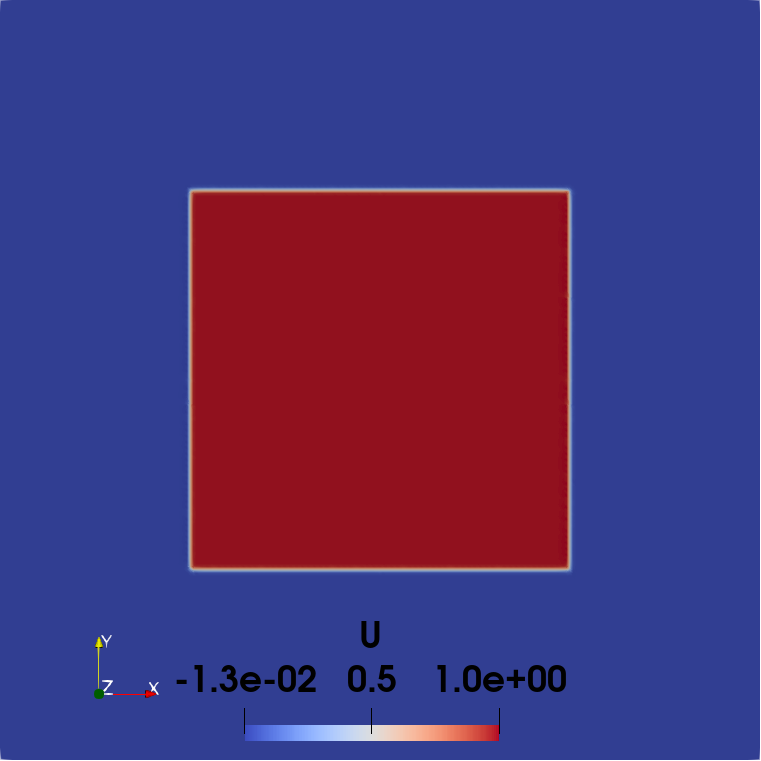
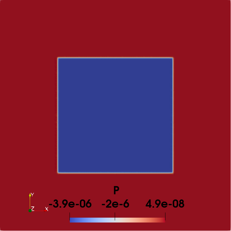
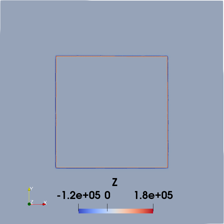
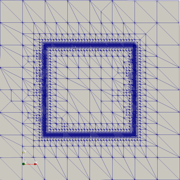
Figure 1: Visualization of the state $u_{\varrho}$, the adjoint state $p_{\varrho}$, the control $z_{\varrho}$, and the adaptive mesh on the cutting plane at time $t=0.5$, where the total #DOFs in space-time is $3,328,617$ at the $58$th adaptive level from $67$ levels (last line in Table 4) corresponding to the regularization parameter $\varrho=2^{-18}$ (Example 4.1.3).

In the last example (Example 4.1.4) of this subsection, we consider the discontinuous target

$$\overline{u}^{\delta}=\overline{u}+2\sqrt{2}\delta\sin(10\pi x_{1})\sin(10\pi x_{2})\sin(10\pi t),$$ (4.3)

that contains some noise in space and time. Here, $\overline{u}$ is one in the inscribed cube $(1/4,3/4)^{3}\subset(0,1)^{3}$ and zero else, and $\delta>0$ is the noise level. For this polluted target, we easily see that $\|\overline{u}^{\delta}-\overline{u}\|_{L^{2}(Q)}=\delta$. To balance the two error contributions we take $h=16\,\delta^{2}$. This ensures an almost optimal convergence with respect to the mesh size $h$, see Table 5.

$\delta$	$h\,\left(=16\cdot\delta^{2}\right)$	$\varrho\,\left(=h^{2}\right)$	$\|\widetilde{u}_{\varrho h}^{\delta}-\overline{u}\|_{L^{2}(Q)}$	eoc
$2^{-3}$	$2^{-2}$	$2^{-4}$	$2.8841$e$-1$
$2^{-3.5}$	$2^{-3}$	$2^{-6}$	$2.0871$e$-1$	$0.47$
$2^{-4}$	$2^{-4}$	$2^{-8}$	$1.4796$e$-1$	$0.50$
$2^{-4.5}$	$2^{-5}$	$2^{-10}$	$1.0535$e$-1$	$0.49$
$2^{-5}$	$2^{-6}$	$2^{-12}$	$7.6837$e$-2$	$0.46$
$2^{-5.5}$	$2^{-7}$	$2^{-14}$	$5.5990$e$-2$	$0.46$

Table 5: Error $\|\widetilde{u}_{\varrho h}^{\delta}-\overline{u}\|_{L^{2}(Q)}$ in the case of a discontinuous target $\overline{u}\in H^{1/2-\varepsilon}(Q)$ containing some noise level $\delta$ (Example 4.1.4).

4.2 Three space dimensions

Now we present some numerical results for the three-dimensional spatial domain $\Omega=(0,1)^{3}$, i.e., $Q=(0,1)^{4}$.

In the first example (Example 4.2.1), we look at the smooth target

$$\overline{u}(x,t)=\sin(\pi x_{1})\sin(\pi x_{2})\sin(\pi x_{3})\sin(\pi t).$$ (4.4)

As predicted by the error estimate (3.14), we observe a second order convergence with respect to the mesh size $h$ when choosing $\varrho=h^{2}$; see Table 6 and Figure 2.

N(#DOFs)	$h=(N/2)^{-1/4}$	$\varrho\,(=h^{2})$	$\|\widetilde{u}_{\varrho h}-\overline{u}\|_{L^{2}(Q)}$
$356$	$2.7378$e$-1$	$7.4953$e$-2$	$2.0985$e$-1$
$630$	$2.3737$e$-1$	$5.6344$e$-2$	$1.7263$e$-1$
$2,986$	$1.6087$e$-1$	$2.5880$e$-2$	$1.2166$e$-1$
$6,930$	$1.3034$e$-1$	$1.6988$e$-2$	$9.3733$e$-2$
$38,114$	$8.5111$e$-2$	$7.2439$e$-3$	$4.7198$e$-2$
$94,146$	$6.7890$e$-2$	$4.6091$e$-3$	$3.2098$e$-2$
$546,562$	$4.3737$e$-2$	$1.9129$e$-3$	$1.4088$e$-2$
$1,400,322$	$3.4570$e$-2$	$1.1951$e$-3$	$8.8652$e$-3$
$8,289,026$	$2.2163$e$-2$	$4.9121$e$-4$	$3.7164$e$-3$
$21,657,090$	$1.7432$e$-2$	$3.0389$e$-4$	$2.2967$e$-3$
$129,165,826$	$1.1155$e$-2$	$1.2444$e$-4$	$9.5061$e$-4$

Table 6: Error $\|\widetilde{u}_{\varrho h}-\overline{u}\|_{L^{2}(Q)}$ in the case of the smooth target $\overline{u}$ given by (4.4) (Example 4.2.1).

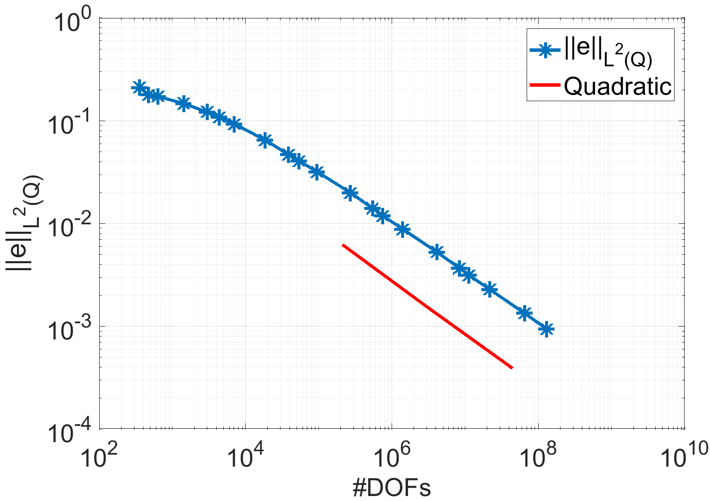
Figure 2: Error $\|e\|_{L^{2}(Q)}=\|\widetilde{u}_{\varrho h}-\overline{u}\|_{L^{2}(Q)}$ in the case of a smooth desired state $\overline{u}\in H_{0}^{1}(Q)\cap H^{2}(Q)$ in three space dimensions (Example 4.2.1).

In the second example (Example 4.2.2), we take a piecewise linear continuous target function $\overline{u}$ being one in the mid point $(1/2,1/2,1/2,1/2)$ and zero in all corner points of $Q=(0,1)^{4}$. In this case we have $\overline{u}\in X\cap H^{3/2-\varepsilon}$, $\varepsilon>0$, and we observe $1.5$ as order of convergence which corresponds to the error estimate (3.17), see Table 7 and Figure 3.

N(#DOFs)	$h=(N/2)^{-1/4}$	$\varrho\,(=h^{2})$	$\|\widetilde{u}_{\varrho h}-\overline{u}\|_{L^{2}(Q)}$
$356$	$2.7378$e$-1$	$7.4953$e$-2$	$2.1510$e$-1$
$630$	$2.3737$e$-1$	$5.6344$e$-2$	$1.7972$e$-1$
$2,986$	$1.6087$e$-1$	$2.5880$e$-2$	$1.3082$e$-1$
$6,930$	$1.3034$e$-1$	$1.6988$e$-2$	$1.0510$e$-1$
$38,114$	$8.5111$e$-2$	$7.2439$e$-3$	$6.1638$e$-2$
$94,146$	$6.7890$e$-2$	$4.6091$e$-3$	$4.5864$e$-2$
$546,562$	$4.3737$e$-2$	$1.9129$e$-3$	$2.4759$e$-2$
$1,400,322$	$3.4570$e$-2$	$1.1951$e$-3$	$1.7766$e$-2$
$8,289,026$	$2.2163$e$-2$	$4.9121$e$-4$	$9.2755$e$-3$
$21,657,090$	$1.7432$e$-2$	$3.0389$e$-4$	$6.5280$e$-3$
$129,165,826$	$1.1155$e$-2$	$1.2444$e$-4$	$3.3636$e$-3$

Table 7: Error $\|\widetilde{u}_{\varrho h}-\overline{u}\|_{L^{2}(Q)}$ in the case of a piecewise linear continuous target $\overline{u}\in X\cap H^{3/2-\varepsilon}(Q)$, $\varepsilon>0$ (Example 4.2.2).

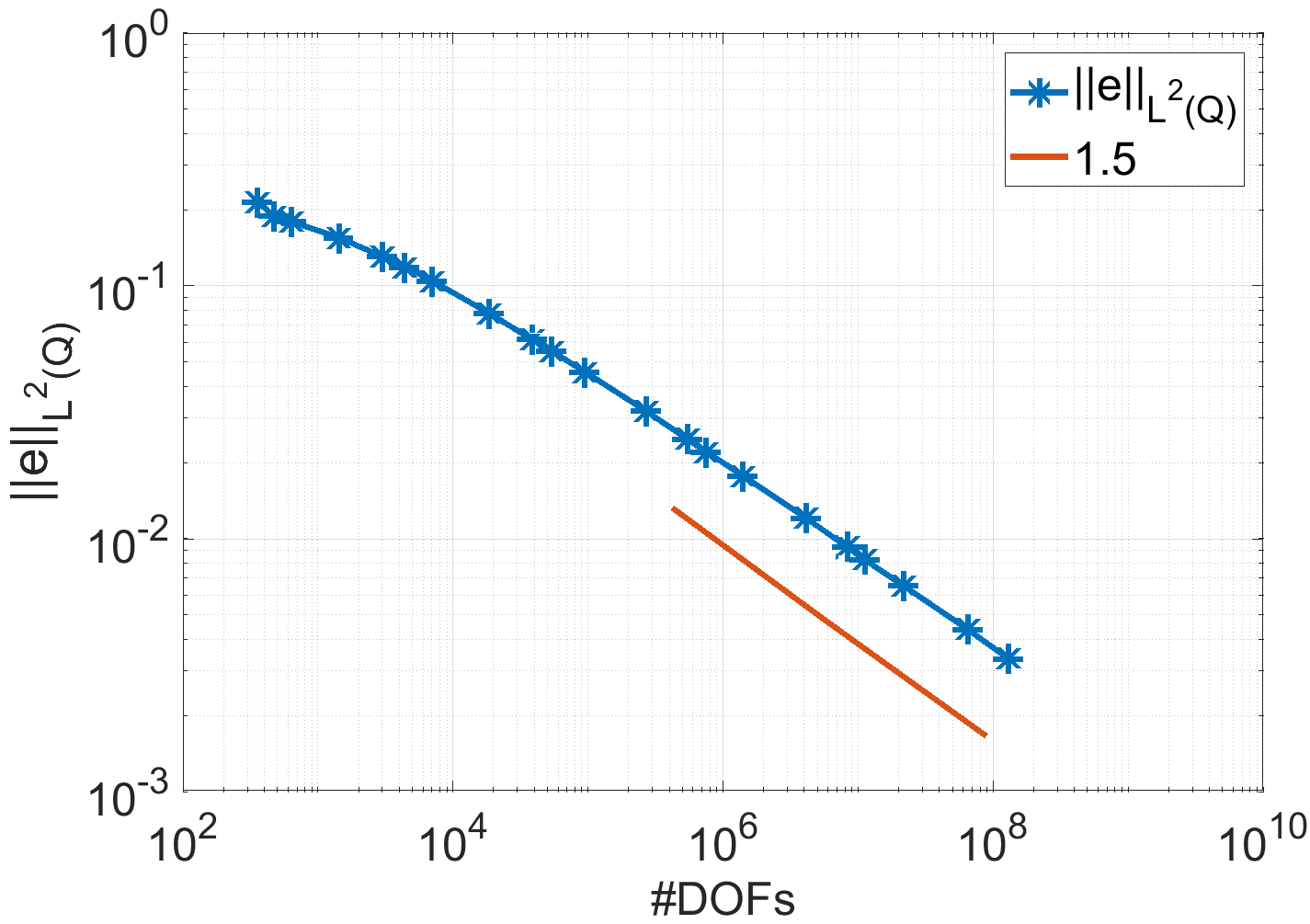
Figure 3: Error $\|e\|_{L^{2}(Q)}=\|\widetilde{u}_{\varrho h}-\overline{u}\|_{L^{2}(Q)}$ in the case of a piecewise linear continuous target $\overline{u}\in X\cap H^{3/2-\varepsilon}(Q)$, $\varepsilon>0$ (Example 4.2.2).

In the third example (Example 4.2.3), we consider a piecewise constant discontinuous target $\overline{u}$ which is one in the inscribed cube $(\frac{1}{4},\frac{3}{4})^{4}$, and zero else. In this case we have $\overline{u}\in H^{1/2-\varepsilon}(Q)$, $\varepsilon>0$. From the numerical results as given in Table 8 we observe $0.5$ for the order of convergence, as expected from the error estimate (3.12), see also Figure 4.

N(#DOFs)	$h=(N/2)^{-1/4}$	$\varrho\,(=h^{2})$	$\|\widetilde{u}_{\varrho h}-\overline{u}\|_{L^{2}(Q)}$
$356$	$2.7378$e$-1$	$7.4953$e$-2$	$2.5099$e$-1$
$630$	$2.3737$e$-1$	$5.6344$e$-2$	$1.9143$e$-1$
$2,986$	$1.6087$e$-1$	$2.5880$e$-2$	$1.8823$e$-1$
$6,930$	$1.3034$e$-1$	$1.6988$e$-2$	$1.7500$e$-1$
$38,114$	$8.5111$e$-2$	$7.2439$e$-3$	$1.4710$e$-1$
$94,146$	$6.7890$e$-2$	$4.6091$e$-3$	$1.3313$e$-1$
$546,562$	$4.3737$e$-2$	$1.9129$e$-3$	$1.0558$e$-1$
$1,400,322$	$3.4570$e$-2$	$1.1951$e$-3$	$9.6592$e$-2$
$8,289,026$	$2.2163$e$-2$	$4.9121$e$-4$	$7.7744$e$-2$
$21,657,090$	$1.7432$e$-2$	$3.0389$e$-4$	$6.8891$e$-2$
$129,165,826$	$1.1155$e$-2$	$1.2444$e$-4$	$5.5284$e$-2$

Table 8: Error $\|\widetilde{u}_{\varrho h}-\overline{u}\|_{L^{2}(Q)}$ in the case of a piecewise constant and discontinuous target $\overline{u}\in H^{1/2-\varepsilon}(Q)$, $\varepsilon>0$ (Example 4.2.3).

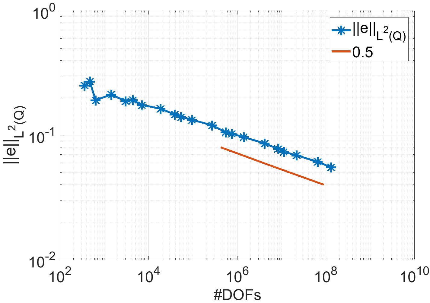
Figure 4: Error $\|e\|_{L^{2}(Q)}=\|\widetilde{u}_{\varrho h}-\overline{u}\|_{L^{2}(Q)}$ in the case of a piecewise constant and discontinuous target $\overline{u}\in H^{1/2-\varepsilon}(Q)$, $\varepsilon>0$ (Example 4.2.3).

5 Conclusions and outlook

We have derived robust space-time finite element error estimates for distributed parabolic optimal control problems with energy regularization. More precisely, we have estimated the $L^{2}(Q)$ norm of the error between the desired state $\overline{u}$ and the computed state $\widetilde{u}_{\varrho h}$ depending on the regularity of the desired state $\overline{u}$. It has been shown that the optimal convergence rate is achieved by the proper scaling $\varrho=h^{2}$ between the regularization parameter $\varrho$ and the mesh size $h$. The theoretical findings are confirmed by several numerical examples in both two and three space dimensions.

The theoretical results are valid for uniform mesh refinement. However, for discontinuous targets $\overline{u}$ and targets that don’t fulfil the boundary or initial conditions, we can expect layers with steep gradients in the solutions as in Example 4.2.3. In this example, we have observed that, for a fixed $\varrho=h^{2}$, the adaptive version needs considerably less unknowns to achieve the same accuracy as the corresponding uniformly refined grid with the finest mesh-size $h$. Since, for adaptively refined grids, the local mesh-sizes are very different, one can also think about a localization of the regularization parameter $\varrho$. Another future research topic is the construction of fast and $\varrho$ robust solvers for the symmetric and indefinite system (4.1) that is equivalent to (3.11); see, e.g., [1, 12, 13, 19]. Finally, the consideration of constraints imposed on the control $z_{\varrho}$ is of practical interest; see, e.g., [17].