Quasi-Bayesian Nonparametric Density Estimation via Autoregressive Predictive Updates

Abstract

Bayesian methods are a popular choice for statistical inference in small-data regimes due to the regularization effect induced by the prior. In the context of density estimation, the standard nonparametric Bayesian approach is to target the posterior predictive of the Dirichlet process mixture model. In general, direct estimation of the posterior predictive is intractable and so methods typically resort to approximating the posterior distribution as an intermediate step. The recent development of quasi-Bayesian predictive copula updates, however, has made it possible to perform tractable predictive density estimation without the need for posterior approximation. Although these estimators are computationally appealing, they struggle on non-smooth data distributions. This is due to the comparatively restrictive form of the likelihood models from which the proposed copula updates were derived. To address this shortcoming, we consider a Bayesian nonparametric model with an autoregressive likelihood decomposition and a Gaussian process prior. While the predictive update of such a model is typically intractable, we derive a quasi-Bayesian update that achieves state-of-the-art results in small-data regimes.

1 Introduction

Modelling the joint distribution of multivariate random variables with density estimators is a central topic in modern unsupervised machine learning research (durkan2019neural; papamakarios2017masked). As well as providing insight into the statistical properties of the data, density estimates are used in a number of downstream applications, including image restoration (zoran2011learning), density-based clustering (scaldelai2022multiclusterkde), and simulation-based inference (lueckmann2021benchmarking). In small-data regimes, Bayesian methods are a popular choice for a wide range of machine learning tasks, including density estimation, thanks to their attractive generalization capacities. For density estimation, the typical Bayesian approach is to target the Bayesian predictive density, $p_{n}(x)=\int f(x|\theta)\pi_{n}(\theta)d\theta,$ where $\pi_{n}$ denotes the posterior density of the model parameters $\theta$ after observing $x_{1},\ldots,x_{n}$, and $f$ denotes the likelihood function.

De Finetti’s representation theorem (de1937prevision; hewitt1955symmetric) states that an exchangeable joint density fully characterises a Bayesian model, which then implies a sequence of predictive densities. Further, fong2021martingale recently showed that a sequence of predictive densities can be sufficient for full Bayesian posterior inference. This provides theoretical motivation for an iterative approach to Bayesian predictive density estimation by updating the predictive $p_{i-1}(x)$ to $p_{i}(x)$ given observation $x_{i}$ for $i=1,\ldots,n$. The idea of recursive Bayesian updates goes back to at least hill1968posterior, but was only recently made more widely applicable through the relaxation of the assumption of exchangeability in favour of conditionally identically distributed (berti2004limit) sequences.

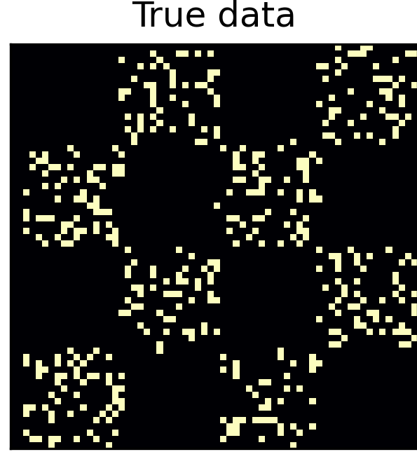
(a)

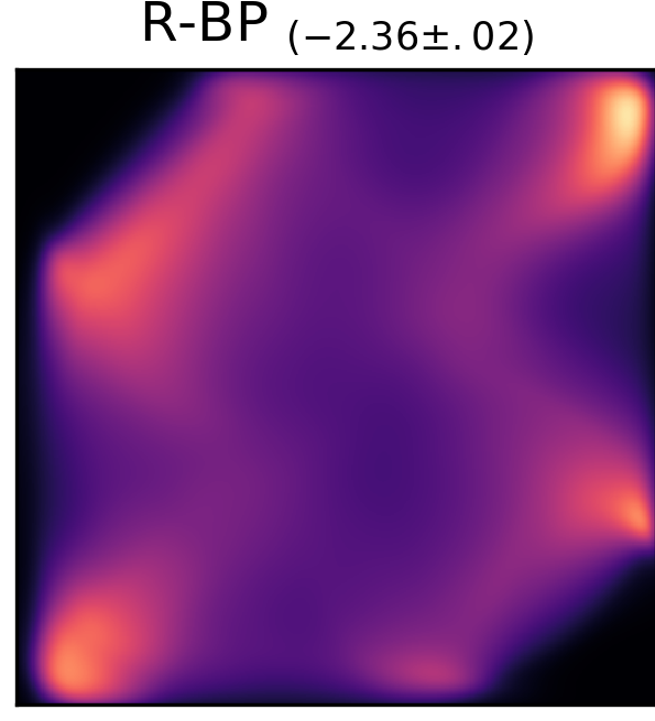
(b)

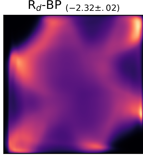
(c)

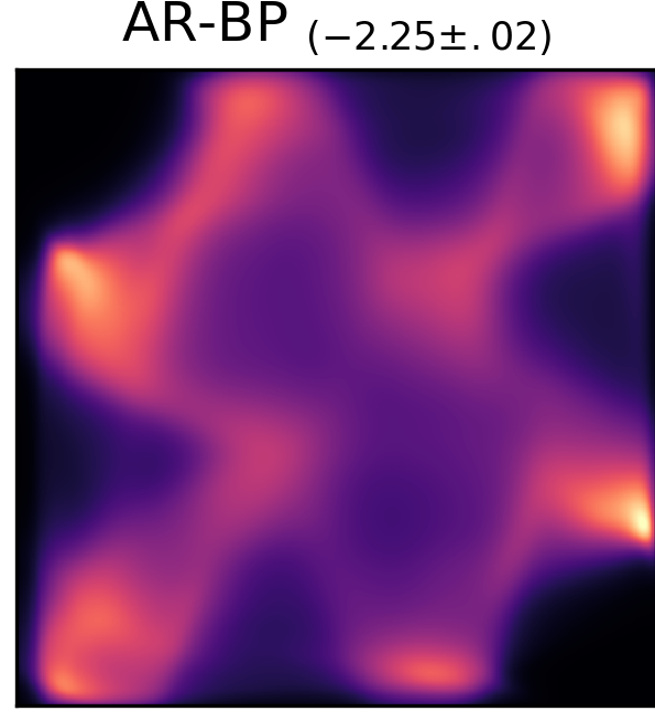
(d)

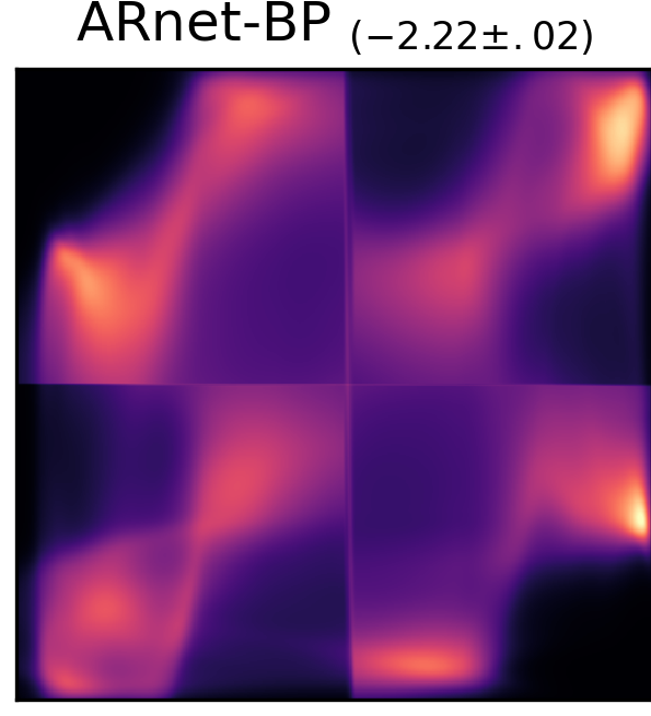
(e)

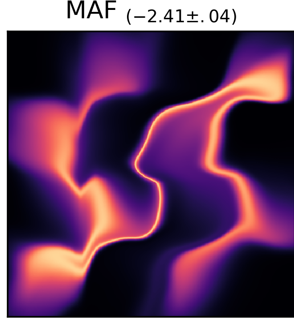
(f)

(g)

Figure 1: Density estimates of 600 observations from a chessboard distribution, reported with mean and standard deviation of test log likelihoods. For larger training sizes, see Supplement 4. Our methods, AR-BP and ARnet-BP, outperform R-BP and AR neural networks.

Here, we focus on a particular class of one-step-ahead predictive updates $p_{i-1}(x)\rightarrow p_{i}(x)$ based on bivariate copulas, which were first introduced by hahn2018recursive for univariate data, and extended by fong2021martingale to the multivariate setting and to regression analyses. This class of updates is inspired by Bayesian models and thus retains many desirable Bayesian properties, such as coherence and regularization. However, we emphasize that the copula updates do not correspond exactly, nor approximately, to a traditional Bayesian likelihood-prior model, and we thus refer to them as quasi-Bayesian (fortini2020quasi). The most related Bayesian density estimator proposed to date, henceforth referred to as the Recursive Bayesian Predictive (R_d-BP), lacks flexibility to model highly complex data distributions (see Figure 1). This is because the existing copula updates rely on a Gaussian copula with a single scalar bandwidth parameter, corresponding to a Bayesian model with a likelihood that factorizes over dimensions. In contrast, popular neural network based approaches, such as masked autoregressive flows (MAFs) (papamakarios2017masked), and rational-quadratic neural spline flows (RQ-NSFs) (durkan2019neural) can struggle in small-data regimes (see Figure 1).

Contributions

This motivates our main contribution, namely the formulation of a more flexible auto-regressive (AR) copula update based on which we propose a new Dirichlet Process Mixture Model (DPMM) inspired density estimator. In particular:

• By considering a DPMM with an AR likelihood and a Gaussian process (GP) prior, we formulate a tractable copula update with a novel data-dependent bandwidth based on the Euclidean metric in data space. Our method, Autoregressive Recursive Bayesian Predictives (AR-BP), outperforms traditional density estimators on tabular data with up to 63 features, and 10,000 samples.

• We observe in practice that the Euclidean metric used in AR-BP can be inadequate for highly non-smooth data distributions. For such cases, we propose using an AR neural network (bengio1999modeling; frey1998graphical; germain2015made; larochelle2011neural) that maps the observations into a latent space before bandwidth estimation. This introduces additional non-linearity through the dependence of the bandwidth on the data, leading to a density estimator, ARnet-BP, that is more accurate on non-smooth densities.

2 Background

We briefly recap predictive density estimation via bivariate copula updates, before describing a particular such update inspired by DPMMs.

2.1 Univariate Predictive Density Updates

To compute predictive densities quickly, hahn2018recursive propose an iterative approach. For $x\in\mathbb{R}$, any sequence of Bayesian posterior predictive densities $p_{i}(x)$ with likelihood $f$ and posterior $\pi_{i}$, conditional on $x_{1:i}$, can be expressed as

$${p_{i}(x)}=\int f(x|\theta)\pi_{i}(\theta)d\theta={p_{i-1}(x)}h_{i}(x,x_{i}),$$ (1)

for some bivariate function $h_{i}(x,x_{i})$ (hahn2018recursive). Rearranging for $h_{i}$, we have

$$h_{i}(x,x_{i}){=}\!\frac{p_{i}(x)}{p_{i-1}(x)}\!\!\overset{(a)}{=}\!\!\frac{p_{i-1}(x|x_{i})}{p_{i-1}(x)}\!\!\overset{(b)}{=}\!\!\frac{p_{i-1}(x,x_{i})}{p_{i-1}(x)p_{i-1}(x_{i})}$$ (2)

where (a) holds by definition, and (b) $p_{i-1}(x,x_{i})=p_{i-1}(x|x_{i})p_{i-1}(x_{i})=p_{i}(x)p_{i-1}(x_{i})$ holds by Bayes’ law. hahn2018recursive show that $h_{i}(x,x_{i})$ is the transformation of a bivariate copula density. A bivariate copula is a bivariate cumulative distribution function (CDF) $C:[0,1]^{2}\rightarrow[0,1]$ with uniform marginal distributions that is used to characterise the dependence between two random variables independent of their marginals:

Theorem 1 (Sklar’s theorem (sklar1959fonctions)).

For any bivariate density $f(y_{1},y_{2})$ with continuous marginal CDFs, $F_{1}(y_{1})$ and $F_{2}(y_{2})$, and marginal densities $f_{1}(y_{1})$ and $f_{2}(y_{2})$, there exists a unique bivariate copula $C$ with density $c$ such that

$$f(y_{1},y_{2})=c\left\{F_{1}(y_{1}),F_{2}(y_{2})\right\}f_{1}(y_{1})f_{2}(y_{2}).$$

Applying the copula factorization from Sklar’s theorem to (2) yields that there exists some bivariate copula density $c_{i}$ such that $p_{i-1}(x,x_{i})=c_{i}\{P_{i-1}(x),P_{i-1}(x_{i})\}p_{i-1}(x)p_{i-1}(x_{i}),$ and thus $h_{i}(x,x_{i})=c_{i}\{P_{i-1}(x),P_{i-1}(x_{i})\},$ where $P_{i-1}$ is the CDF corresponding to the predictive density $p_{i-1}$. Given prior $\pi$ and likelihood $f$, Equation 2 suggests that the update function can be written as

$$h_{i}(x,x_{i})=\frac{\int f(x|\theta)f(x_{i}|\theta)\pi_{i-1}(\theta)d\theta}{\int f(x|\theta)\pi_{i-1}(\theta)d\theta\int f(x_{i}|\theta)\pi_{i-1}(\theta)d\theta}\cdot$$

For each Bayesian model, there is thus a unique sequence of symmetric copula densities $c_{i}(u,v)=c_{i}(v,u)$. This sequence has the property that $c_{n}(\cdot,\cdot)\rightarrow 1$ converges to a constant function as $n\rightarrow\infty$, ensuring that the predictive density converges asymptotically with sample size $n$.

In general, the above equation is intractable due to the posterior so it is not possible to compute the iterative update in (1) for fully Bayesian models. Alternatively, we will consider sequences of $h_{i}$ that match the Bayesian model for $i=1$, but not for $i>1$. As mentioned above, this copula update no longer corresponds to a Bayesian model, nor are the resulting predictive density estimates approximations to a Bayesian model. Nevertheless, if the copula updates are conditionally identically distributed, they still exhibit desirable Bayesian characteristics such as coherence and regularization, and are hence referred to as quasi-Bayes. Please refer to berti2004limit for details.

2.2 Multivariate Predictive Density Updates

The above arguments cannot directly be extended to multivariate $x\in\mathbb{R}^{d}$ since $h_{i}$ cannot necessarily be written as $c_{i}\{P_{i-1}(x),P_{i-1}(x_{i})\}$ for $d>1$. However, (2) still holds, and recursive predictive updates with bivariate copulas as building blocks can be derived explicitly given a pre-defined likelihood model and a prior, which we now exhibit.

hahn2018recursive and fong2021martingale propose to use DPMMs as a general-use nonparametric model. The DPMM (escobar1988estimating; escobar1995bayesian) can be written as

$$f(x|G)=\int_{\Theta}K(x|\theta)\,dG(\theta),\text{ with }G\sim\text{DP}(c,G_{0})$$ (3)

where $\theta\in\Theta=\mathbb{R}^{d}$ are parameter vectors, the prior assigned to $G$ is a Dirichlet process (DP) prior with base measure $G_{0}$ and concentration parameter $c>0$ (ferguson1973bayesian), and $K(x|\theta)$ is a user-specified kernel (not to be confused with the covariance function of a GP). In particular, fong2021martingale consider the base measure $G_{0}=\mathcal{N}(0,\tau^{-1}I_{d})$ for some precision parameter $\tau\in\mathbb{R}_{>0}$, and the factorized kernel $K(x|\theta)=\mathcal{N}(x|\theta,I_{d})$ where $I_{d}$ is the $d$-dimensional identity matrix. The likelihood is then

$$f(x|G)=\int\prod_{j=1}^{d}\mathcal{N}\left(x^{j}\mid\theta^{j},1\right)dG({\theta}),$$ (4)

where the dimensions of $x$ are conditionally independent given $\theta$. Following hahn2018recursive, we denote the dimension $j$ of a vector $y$ with $y^{j}$. We note that the strong assumption of a factorised kernel form drastically impacts the performance of the regular DPMM and also influences the form and modelling capacity of the corresponding copula update.

This model inspires the following recursive predictive density update $p_{i}(x)=h_{i}(x,x_{i})p_{i-1}(x)$ for which the first $d^{\prime}\in\{1,\ldots,d\}$ marginals take on the form

$$\frac{p_{i}({x}^{1:d^{\prime}})}{p_{i-1}\left(x^{1:d^{\prime}}\right)}\!= 1\!-\!\alpha_{i}\!+\!\alpha_{i}\!\prod_{j=1}^{d^{\prime}}\!c\left(u_{i-1}^{j}(x^{j}),v_{i-1}^{j};\rho_{0}\right),$$ (5)

$$u_{i-1}^{j}(x^{j}):= P_{i-1}\left(x^{j}\mid x^{1:j-1}\right),$$

$$v_{i-1}^{j}:= P_{i-1}\left(x_{i}^{j}\mid x_{i}^{1:j-1}\right),$$

where $c(u,v;\rho_{0})$ is the bivariate Gaussian copula density with correlation $\rho_{0}=1/(1+\tau)$, $p_{0}$ can be any chosen prior density, and $\alpha_{i}=\left(2-\frac{1}{i}\right)\frac{1}{i+1}$ (see Supplement A and fong2021martingale). Note that the above update requires a specific ordering of the feature dimensions, and the Gaussian copula follows from the Gaussian distribution in the kernel and $G_{0}$ for the DPMM. Unlike the DPMM, there are now no underlying parameters (beyond $\rho_{0}$) in the copula update as we have integrated out $\theta$, so we do not carry out clustering directly. While $\rho_{0}$ is a scalar here, fong2021martingale also consider the setting with a distinct bandwidth parameter for each dimension. We refer to these recursive Bayesian predictives as R_d-BP, or simply R-BP if the dimensions share a single bandwidth.

3 AR-BP: Autoregressive Bayesian Predictives

For smooth data distributions, the recursive update defined in (5) generates density estimates that are highly competitive against other popular density estimation procedures such as kernel density estimation (KDE) and DPMM (fong2021martingale). Moreover, the iterative updates provide a fast estimation alternative to fitting the full DPMM through Markov chain Monte Carlo (MCMC). When considering more structured data, however, performance suffers due to the choices of the factorized kernel $K(\cdot|\theta)=\mathcal{N}(\cdot|\theta,I_{d})$ and simple base measure $G_{0}=\mathcal{N}(0,\tau^{-1}I_{d})$ in the DPMM. These choices induce a priori independence between the data dimensions, and are thus insufficiently flexible to capture more complex dependencies.

3.1 Bayesian Model Formulation

We therefore propose employing more general kernels and base measures in the DPMM and show that these inspire a more general tractable recursive predictive update. In particular, we allow the kernel to take on an autoregressive structure

$$K(x|\theta)=\prod_{j=1}^{d}\mathcal{N}\left(x^{j}\mid\theta^{j}\left(x^{1:j-1}\right),1\right),$$ (6)

where $\theta^{j}:\mathbb{R}^{j-1}\rightarrow\mathbb{R}$ is now an unknown mean function, and not scalar, for dimension $x^{j}$, which we allow to depend on the previous $j-1$ dimensions of $x$. Thus, specifying our DPMM requires a base measure supported on the function space in which $(\theta^{1},\dots,\theta^{d})$ is valued. We specify this base measure as a product of independent GP priors on the functional parameters

$$\theta^{j}\sim\text{GP}(0,\tau^{-1}k^{j})\text{ for }j=1,...,d$$ (7)

where $k^{j}:\mathbb{R}^{j-1}\times\mathbb{R}^{j-1}\rightarrow\mathbb{R}$ and $k^{j}$ can be any given covariance function that takes as input a pair of ${x}^{1:j-1}$ values. In practice, we use the same functional form of $k$ for each $j$, so we will drop the superscript $j$. For later convenience, we have also written the scaling term $\tau^{-1}$ explicitly. We highlight that for $j=1$, $\theta^{1}\sim\mathcal{N}(0,\tau^{-1})$. Under this choice, the mean of the normal kernels in the DPMM for each dimension $j$ is thus a flexible function of the first $j-1$ dimensions $x^{1:j-1}$, on which we elicit independent GP priors. The conjugacy of the GP with the Gaussian DPMM kernel in (6) is crucial for deriving a tractable density update.

Remark.

The proposed DPMM kernel in (6) is in fact more flexible than a general multivariate kernel, $K(x\mid\theta)=\mathcal{N}(x\mid\theta,\Sigma)$. This is because the multivariate kernel also implies an AR form like (6) but where the parameters $\theta^{j}$ are restricted to be linear in $x^{1:j-1}$; see wade2014predictive for details.

3.2 Iterative Predictive Density Updates

Computing the Bayesian posterior predictive density induced by the DPMM with kernel given by (6) and base measure given by (7) through posterior estimation is intractable and requires MCMC. However, as before, we can utilize the model to derive tractable iterative copula updates. In Supplement LABEL:app:ar-deriv, we derive the corresponding recursive predictive density update $p_{i}(x)=h_{i}(x,x_{i})p_{i-1}(x)$ for the first $d^{\prime}$ marginals and show that it takes on the form

$$\frac{p_{i}({x}^{1:d^{\prime}})}{p_{i-1}(x^{1:d^{\prime}})}= 1-\alpha_{i}+\alpha_{i}\cdot$$ (8)

$$\prod_{j=1}^{d^{\prime}}c\left(u_{i-1}^{j}(x^{j}),v_{i-1}^{j};\rho^{j}(x^{1:j-1},x_{i}^{1:j-1})\right),$$

with $u_{i-1}^{j}(x^{j}),v_{i-1}^{j}$ defined as in (5), $\alpha_{i}=\left(2-\frac{1}{i}\right)\frac{1}{i+1}$, and the bandwidth given by

$$\rho^{j}(x^{1:j-1},x_{i}^{1:j-1})=\rho_{0}k\left(x^{1:j-1},x_{i}^{1:j-1}\right),$$ (9)

for $\rho_{0}=1/(1+\tau)$, and $\rho_{i}^{1}=\rho_{0}$. Where appropriate, we henceforth drop the argument $x$ for brevity. The conditional CDF s $u_{i-1}^{j}$ can also be computed through an iterative closed form expression similarly to (8) (Supplement B.3). Please see Figure 2 for a simplified overview of the density estimation pipeline.

Figure 2: Simplified summary of AR-BP. We repeat the training update for each train datum $x_{i}$ to estimate $v_{i}^{j}=P_{i-1}(x^{1:j}_{i})$. These are needed at test time to update from $p_{i-1}(z)\rightarrow p_{i}(z)$. All steps are averaged over different feature and sample permutations. The main step that induces autoregression in the observations is highlighted pink. Please see Supplement B.3 for detailed algorithms.

Note that the estimation is identical to the update given in (5) induced by the factorized DPMM kernel, except for the main difference that the bandwidth $\rho$ is no longer a constant, but is now data-dependent. More precisely, the bandwidth for dimension $j$ is a transformation of the GP covariance function $k$ on the first $j-1$ dimensions. The additional flexibility afforded by the inclusion of $k$ enables us to capture more complex dependency structures, as we do not enforce a-priori independence between the dimensions of the parameter $\theta$. Similarly to the extension of R-BP to R_d-BP, we can also define AR_d-BP by introducing dimension dependence in $\rho_{0}$. Finally, we highlight that extending R-BP to mixed data is possible as given in Appendix E.1.3 of fong2021martingale, which also extends naturally to AR-BP.

Remark.

The data-dependent bandwidth also appears when starting from other Bayesian nonparametric models, such as dependent DP s and GPs (see Supplement LABEL:app:gp for the derivation).

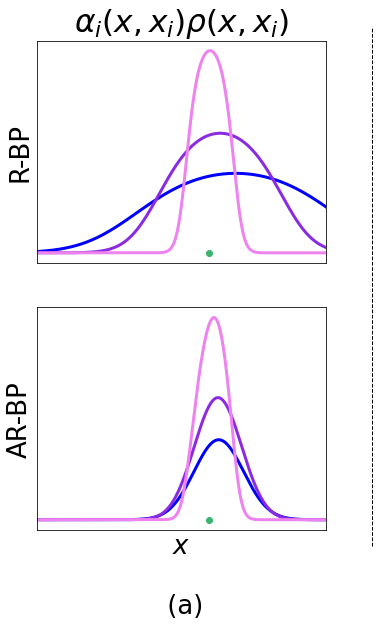
(a)

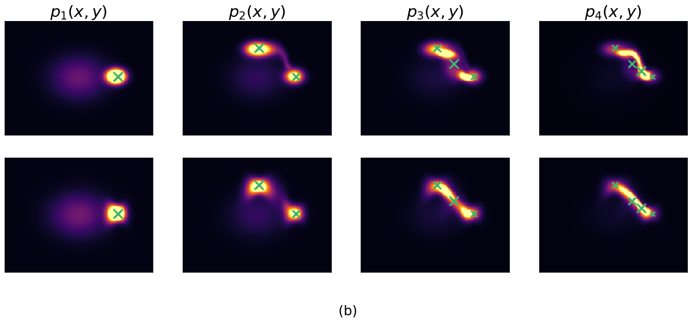
(b)

Figure 3: (a) Plots of $\alpha_{i}(x,x_{i})\rho(x,x_{i})$ for R-BP and AR-BP for $\rho_{0}\in\{0.5,0.7,0.95\}$ ( , , ) with new observation $x_{i}$ ( ). Note that $\rho(x,x_{i})=\rho_{0}$ for R-BP, and $\ell=1$ for AR-BP. (b) Density plots for R-BP and AR-BP trained on 4 sequential data points ( ). Both figures show that the update of R-BP, unlike AR-BP, is not centred around the new datum.

Our approach can be viewed as a Bayesian version of an online KDE procedure. To see this, note that a KDE trained on $i-1$ observations – yielding the density estimate $q_{i-1}(x)$ – can be updated after observing the $i^{th}$ observation $x_{i}$ via $q_{i}(x)=(1-\alpha_{i})q_{i-1}(x)+\alpha_{i}d\left(x,x_{i}\right)$, where $\alpha_{i}=1/i$ and $d(\cdot,\cdot)$ denotes the kernel of the KDE. Rather than adding a weighted kernel term directly, AR-BP instead adds an adaptive kernel that depends on a notion of distance between $x$ and $x_{i}$ based on the predictive CDF s conditional on $x_{1:i-1}$.

To better understand the importance of the data-dependent bandwidth, we compare the conditional predictive mean of R-BP and AR-BP in the bivariate setting $X\times Y$. Under the simplifying assumption of Gaussian predictive densities, we show in Supplement LABEL:app:cond_mean that the conditional mean of $Y\mid X$ is given by

$$\mu_{i}(x) =\mu_{i-1}(x)+\alpha_{i}(x,x_{i})\rho(x,x_{i})(y_{i}-\mu_{i-1}(x_{i})),$$

$$\alpha_{i}(x,x_{i}) =\frac{\alpha_{i}c(P_{i-1}(x),P_{i-1}(x_{i});\rho)}{1-\alpha_{i}+\alpha_{i}c(P_{i-1}(x),P_{i-1}(x_{i});\rho)}.$$

Note that $\rho(x,x_{i})=\rho_{0}$ for R-BP. Intuitively, the updated mean is the previous mean plus a residual term at $y_{i}$ scaled by some notion of distance between $x$ and $x_{i}$. For R-BP, this distance between $x$ and $x_{i}$ depends only on their predictive CDF values through $\alpha_{i}(x,x_{i})$. This can result in undesirable behaviour as shown in the upper plot in Figure 3(a), where the peak of $\alpha_{i}(x,x_{i})$, as a function of $x$, is not centred at $x_{i}$. Counterintuitively, there is thus an $x>x_{i}$ where $\mu_{i}(x)$ is updated more than at the actual observed $x=x_{i}$. This follows from the lack of focus on conditional density estimates for R-BP, which is alleviated by AR-BP. In the AR case, $\rho(x,x_{i})$ takes into account the Euclidean distance between $x$ and $x_{i}$ in the data space. We see in the lower plot in Figure 3(a) that the peak is closer to $x_{i}$. Figure 3(b) further demonstrates this difference on another toy example - we see that R-BP struggles to fit a linear conditional mean function for $n=4$, focussing density in data sparse regions, while AR-BP succeeds to assign significant density only to points on the data manifold.

Training the update parameters

In order to compute the predictive density $p_{n}(x^{*})$, we require the vector of conditional CDF s $[v_{1}^{j},\ldots,v_{n-1}^{j}]$ where $v_{i}^{j}=P_{i}(x_{i+1}^{j}\mid x_{i+1}^{1:j-1})$. Given a bandwidth parameterization, obtaining this vector thus amounts to model-fitting, and each $v_{i}^{j}$ requires $i-1$ iterations (Supplement B.3), for $i\in\{1,\ldots,n\}$. We note that the order of samples and dimensions influences the prediction performance in AR density estimators (vinyals2015order). In practice, averaging over different permutations of these improves performance (Supplement B.3). Full implementation details can be found in Supplement LABEL:app:algs.

Computational complexity

The above procedure results in a computational complexity of $\mathcal{O}(Mdn^{2})$ at the training stage where $M$ is the number of permutations. At test time, we have already obtained the necessary conditional prequential CDFs $v_{n}^{j}$ in computing the prequential log-likelihood above. As a result, we have a computational complexity $\mathcal{O}(Mdn)$ for each test observation. Note that the introduction of a data-dependent bandwidth does not increase the computational complexity at train or test time relative to R-BP and only adds a negligible factor to the computational time for the calculation of the bandwidth.

3.3 Bandwidth Parameterisation

The choice of covariance function in (7) provides substantial modelling flexibility in our AR-BP framework. Moreover, the additional parameters associated with the covariance function allow us to tune the implied covariance structure according to the observed data. This formulation enables us to draw upon the rich literature on the choice of covariance functions for Gaussian processes (williams2006gaussian). For simplicity we only consider the most popular such choice here, but study the more flexible rational-quadratic covariance in Supplement LABEL:app:exp-add. The radial basis function (RBF) covariance function is defined as $k_{\ell}(x^{1:j-1},x^{{}^{\prime}1:j-1})=\exp[-\sum_{\kappa=1}^{j-1}\{({x^{\kappa}-x^{{}^{\prime}\kappa}})/{\ell^{\kappa}}\}^{2}],$ where $\ell\in\mathbb{R}^{d-1}_{>0}$ is the length scale.

Neural parameterisation

As we saw in the motivating example of the density estimation of a chessboard distribution in Figure 1, the RBF kernel can restrict the capacity of the predictive density update to capture intricate nonlinearities if the training data size is not sufficient. While the parameterization of the bandwidth in (9) was initially derived via the first predictive update for a DPMM, all we require is that the bandwidth function $\rho^{j}:\mathbb{R}^{j-1}\times\mathbb{R}^{j-1}\to\mathbb{R}$ lies in (0,1). We would also like $\rho^{j}(x^{1:j-1},x^{{}^{\prime}1:j-1})$ to take larger values when $x^{1:j-1}$ and $x^{{}^{\prime}1:j-1}$ are ‘close’ in some sense. Motivated by this observation, we now consider more expressive bandwidth functions that can lead to increased predictive performance. In particular, we formulate an AR neural network ${f}_{w}:\mathbb{R}^{d}\rightarrow\mathbb{R}^{d\times d^{\prime}}$ for $d^{\prime}\in\mathbb{N}$ with the property that the $j^{th}$ row of the output depends only on the first $j-1$ dimensions of the input. Let $Z={f}_{w}\left(x\right)$ and denoting ${z}^{j}$ to be the $j^{th}$ row of the matrix $Z$, the covariance function is then computed as $\rho^{j}(x^{1:j-1},x^{{}^{\prime}1:j-1})=\rho_{0}\exp(-\sum_{\kappa=1}^{j-1}\lvert\lvert{{z}}^{\kappa}-{z}^{{}^{\prime}\kappa}\rvert\rvert^{2}_{2}).$

Numerous AR neural network models have been extensively used for density estimation (dinh2014nice; huang2018neural; kingma2016improved). In our experiments, we use a relatively simple model with parameter sharing inspired by NADE, an AR neural network designed for density estimation (larochelle2011neural). More advanced properties like the permutation invariance of MADE (papamakarios2017masked) create an additional overhead that cannot be used in the copula formulation as the predictive update is not permutation-invariant. We refer to Bayesian predictive densities estimated using AR neural networks as ARnet Bayesian predictives (ARnet-BP).

Tuning the bandwidth function

Recall that the bandwidths $\rho_{i}(\cdot,\cdot)$ are parameterised by $\rho_{0}$ and the parameters of the chosen covariance functions or neural embedders. For AR-BP, these are the length scales $\ell$ of the RBF covariance function, while for ARnet-BP, these are the parameters $w$ of the AR neural network. We fit these tunable parameters in a data-driven approach by maximising the prequential (dawid1997prequential) log-likelihood $\sum_{i=1}^{n}\log p_{i-1}(x_{i})$ which is analogous to the Bayesian marginal likelihood – the tractable predictive density allows us to compute this exactly, and this approach is analogous to empirical Bayes. Specifically, we use gradient descent optimisation with Adam, sampling a different random permutation of the training data at each optimisation step (Supplement B.3).

4 Related Work

Our work falls into the broad area of multivariate density estimation (scott2015multivariate). While AR networks have been previously used directly for the task of density estimation (bengio1999modeling; germain2015made; larochelle2011neural), we use them to elicit a data-dependent bandwidth in the predictive update to mitigate the smoothing effect observed in AR-BP. Neural network based approaches, however, often underperform in small-data regimes. Deep learning approaches that do target few-shot density estimation require complex meta-learning and pre-training pipelines (gu2020ensemble; reed2017few).

Our work directly extends the contributions of hahn2018recursive and fong2021martingale through an alternative specification of the nonparametric Bayesian model in the recursive predictive update scheme. R-BP has recently been used for nonparametric solvency risk prediction (hong2019real), and survival analysis (fong2022predictive). berti2021bayesian; berti2021class; berti2004limit also focus on univariate predictive updates in the Bayesian nonparametric paradigm, specifically exploring the use of the conditionally identically distributed condition as a relaxation of the standard exchangeability assumption. Other studies have investigated quasi-Bayesian updates in the special case of the mixing distribution in nonparametric mixture models (dixit2022prticle; fortini2020quasi; martin2018nonparametric; tokdar2009consistency), though these typically focus on univariate or low-dimensional spaces. See also martin2021survey for a survey.

Finally, copulas are a well-studied tool for modelling the correlations in multivariate data (see e.g. kauermann2013flexible; ling2020deep; nelsen2007introduction). Copula density estimation aims to construct density estimates whose univariate marginals are uniform (gijbels1990estimating), and often focus on modelling strong tail dependencies (wiese2019copula). In contrast, we employ bivariate copulas for generic multivariate density estimation as a tool to model the correlations between subsequent subjective predictive densities, rather than across the data dimensions directly.

Table 1: Average NLL with standard error over five runs on data sets analysed by fong2021martingale.

	WINE	BREAST	PARKIN	IONO	BOSTON
n/d	89/12	97/14	97/16	175/30	506/13
KDE	${13.69_{\pm 0.00}}$	${10.45_{\pm 0.24}}$	${12.83_{\pm 0.27}}$	${32.06_{\pm 0.00}}$	${8.34_{\pm 0.00}}$
DPMM (Diag)	${17.46_{\pm 0.6}}$	${16.26_{\pm 0.71}}$	${22.28_{\pm 0.66}}$	${35.30_{\pm 1.28}}$	${7.64_{\pm 0.09}}$
DPMM (Full)	${32.88_{\pm 0.82}}$	${26.67_{\pm 1.32}}$	${39.95_{\pm 1.56}}$	${86.18_{\pm 10.22}}$	${9.45_{\pm 0.43}}$
MAF	${39.60_{\pm 1.41}}$	${10.13_{\pm 0.40}}$	${11.76_{\pm 0.45}}$	${140.09_{\pm 4.03}}$	${56.01_{\pm 27.74}}$
RQ-NSF	${38.34_{\pm 0.63}}$	${26.41_{\pm 0.57}}$	${31.26_{\pm 0.31}}$	${54.49_{\pm 0.65}}$	${-2.20_{\pm 0.11}}$
R-BP	${13.57_{\pm 0.04}}$	${7.45_{\pm 0.02}}$	${9.15_{\pm 0.04}}$	${21.15_{\pm 0.04}}$	${4.56_{\pm 0.04}}$
Rd-BP	${13.32_{\pm 0.01}}$	${6.12_{\pm 0.05}}$	${7.52_{\pm 0.05}}$	${19.82_{\pm 0.08}}$	${-13.50_{\pm 0.59}}$
AR-BP	${13.45_{\pm 0.05}}$	${6.18_{\pm 0.05}}$	${8.29_{\pm 0.11}}$	${17.16_{\pm 0.25}}$	${-0.45_{\pm 0.77}}$
ARd-BP	$\bm{13.22_{\pm 0.04}}$	$\bm{6.11_{\pm 0.04}}$	$\bm{7.21_{\pm 0.12}}$	${16.48_{\pm 0.26}}$	$\bm{-14.75_{\pm 0.89}}$
ARnet-BP	${14.41_{\pm 0.11}}$	${6.87_{\pm 0.23}}$	${8.29_{\pm 0.17}}$	$\bm{15.32_{\pm 0.35}}$	${-5.71_{\pm 0.62}}$

Figure 4: Average NLL and standard errors over 10 runs for training sets of different size. Our models outperform neural methods for data sets up to 10,000 samples.

5 Experiments

We demonstrate the benefits of AR-BP, AR_d-BP and ARnet-BP for density estimation and prediction tasks in an experimental study with five baseline approaches and 13 different data sets. The code and data used is provided in the Supplementary Material. See Supplement C for additional experimental details and results, including a sensitivity study, an ablation study, further illustrative examples, a preliminary investigation into image examples, and an empirical study of the computational complexity of the proposed methods.

5.1 Density Estimation

We compared our models against KDEs (parzen1962estimation), DPMMs (rasmussen1999infinite), MAFs (papamakarios2017masked) and RQ-NSFs (durkan2019neural). The hyperparameters of the baselines were tuned with cross-validation. Unless otherwise specified, we use respectively 10 permutations over samples and features to average the quasi-Bayesian estimates. We did not see substantial improvements with more permutations. We use the same few hyperparameters (initialisation of $rho,l_{1},\ldots,l_{d}$, number of permutations, neural network architecture, and learning rate) on all data sets as our method is robust to their choice. See Supplement C.1 for further information.

Data sets analysed by fong2021martingale

See Table 4 for the negative log-likelihood (NLL) estimated on five UCI data sets (asuncion2007uci) of small size with up to 506 samples, as investigated by fong2021martingale. Our proposed methods display highly competitive performance: AR_d-BP achieved the best test NLL on four of the data sets, while ARnet-BP prevailed on ionosphere.

Table 2: Average NLL over five runs reported with standard error for supervised tasks

(b)

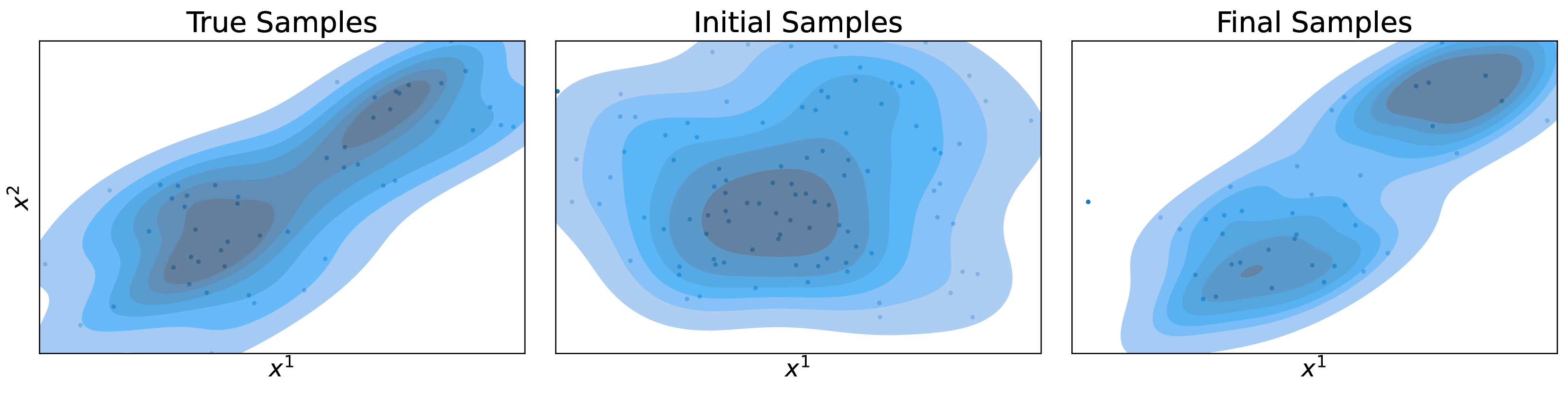
(c)

Figure 5: 100 samples generated from AR_d-BP trained on 50 samples from a GMM with 4 components. All three sampling approaches manage to preserve the multi-modal data distribution.

B.2 Supervised Learning

We briefly recap how joint density estimation can be extended to conditional supervised learning (regression and classification), as outlined by fong2021martingale. Please see Supplement LABEL:app:deriv_suplearn for the derivation. Given fixed design points ${x}_{1:n}$ and random response $y_{1:n}$, the problem at hand is to infer a family of conditional densities $\{f_{x}(y):{{x}\in\mathbb{R}^{d}}\}$.

B.2.1 Regression

For the regression case, fong2021martingale posit a Bayesian model with the nonparametric likelihood being a covariate-dependent stick-breaking DPMM:

$$f_{G_{x}}({y})=\int\mathcal{N}(y\mid\theta,1)\,dG_{{x}}({\theta}),\quad G_{x}=\sum_{k=1}^{\infty}w_{k}({x})\,\delta_{\theta_{k}^{*}},$$ (16)

where $w_{k}(\mathbf{x})$ follows an ${x}$-dependent stick-breaking process. Our contribution is to assume an autoregressive factorisation of the kernel and independent GP priors on $\theta_{k}^{*}$. See Supplement LABEL:app:deriv_copula_regression for the derivation of the predictive density update that is now given by

$$p_{i}(y\mid x)=\left[1-\beta_{i}(x,x_{i})+\beta_{i}(x,x_{i})\,c\left\{P_{i-1}(y\mid x),P_{i-1}(y_{i}\mid x_{i});\rho_{i}(x)\right\}\right]\,p_{i-1}(y\mid x),$$ (17)

where $\rho_{i}(x)=\rho^{d+1}_{i}(x)$ and $\beta$ as in (LABEL:eq:condit_alpha).

B.2.2 Classification

For $y_{i}\in\{0,1\}$, fong2021martingale assume a beta-Bernoulli mixture. As explained in Supplement LABEL:app:deriv_copula_classification and fong2021martingale, this gives the same update as in the regression setting with the difference that the copula $c$ in (17) is replaced with

$$b\{q_{i-1},r_{i-1};\rho_{i}(x)\} =\begin{dcases}1-\rho_{i}(x)+\rho_{i}(x)\,\frac{q_{i-1}\wedge r_{i-1}}{q_{i-1}\,r_{i-1}}&\quad\text{if }y=y_{i}\vspace{2mm}\\ 1-\rho_{i}(x)+\rho_{i}(x)\,\frac{q_{i-1}-\{q_{i-1}\wedge(1-r_{i-1})\}}{q_{i-1}\,r_{i-1}}&\quad\text{if }y\neq y_{i},\end{dcases}$$

where $\rho_{i}(x)=\rho^{d+1}_{i}(x),q_{i-1}=p_{i-1}(y\mid\mathbf{x}),r_{i-1}=p_{i-1}(y_{i}\mid\mathbf{x}_{i})$ and $\rho_{y}\in(0,1)$.

B.3 Implementation Details

Please see Algorithm 1 for the full estimation procedure, Algorithm B.3 for the optimisation of the bandwidth parameters, Algorithm B.3 for the fitting procedure of the predictive density updates, and eventually Algorithm B.3 for the steps during test-time inference. All algorithms are written for one specific permutation of the dimensions, and are repeated for different permutations.

Note that at both training time and test time, we need to consider the updates on the scale of the CDF s, that is for the terms such as $u_{i}^{j}(x^{j})$, which appear in the update step (8). Given

$$u_{i}^{j}(x^{j})=P_{i}(x^{j}|x^{1:j-1})=\int_{-\infty}^{x^{j}}{p_{i}(x^{1:j-1},x^{{}^{\prime}j})}/{p_{i}(x^{1:j-1})}dx^{{}^{\prime}j},$$

and (8), the CDF s $u_{i}^{j}(x^{j})$ take on the tractable update

$$\displaystyle{u_{i}^{j}=\left\{(1-\alpha_{i})u_{i-1}^{j}+\alpha_{i}H\left(u_{i-1}^{j},v_{i-1}^{j};\rho_{i}^{j}\right)\prod_{r=1}^{k-1}c\left(u_{i-1}^{r},v_{i-1}^{r};\rho_{i}^{r}\right)\right\}\frac{p_{i-1}\left(x^{1:k-1}\right)}{p_{i}\left(x^{1:k-1}\right)}},$$ (18)

and set $v_{i-1}^{j}=u_{i-1}^{j}(x_{i})$ which holds by definition, where we dropped the argument $x$ for simplicity from $\rho_{i}^{j}$ and $u_{i}^{j}$, and $H(u,v;\rho)$ denotes the conditional Gaussian copula distribution with correlation $\rho$, that is

$$H(u,v;\rho)=\int_{0}^{u}c(u^{\prime},v;\rho)du^{\prime}=\Phi\left\{\frac{\Phi^{-1}(u)-\rho\Phi^{-1}(v)}{\sqrt{1-\rho^{2}}}\right\}\cdot$$

The Gaussian copula density $c(u,v;\rho)$ is given by

$$c(u,v;\rho)=\frac{\mathcal{N}_{2}\left\{\Phi^{-1}(u),\Phi^{-1}(v)\mid 0,1,\rho\right\}}{\mathcal{N}\{\Phi^{-1}(u)\mid 0,1\}\mathcal{N}\{\Phi^{-1}(v)\mid 0,1\}},$$

where $\Phi$ is the normal CDF, and $\mathcal{N}_{2}$ is the standard bivariate density with correlation $\rho\in(0,1)$.

Ordering

Note that the predictive density update depends on the ordering of both the training data and the dimensions. This permutation dependence is not an additional assumption on the data generative process, and the only implication is that the subset of ordered marginal distributions continue to satisfy (5) (main paper). In the absence of a natural ordering of the training samples or the dimensions, we take multiple random permutations, observing in practice that the resulting averaged density estimate performs better. More precisely, for a given permutation of the dimensions, we first tune the bandwidth parameters, and then calculate density estimates based on multiple random permutations of the training data. We then average over each of the resulting estimates to obtain a single density estimate for each dimension permutation, and subsequently take the average across these estimates to obtain the final density estimate. Importantly, our method is parallelizable over permutations and thus able to exploit modern multi-core computing architectures.

Algorithm 1 Full density estimation pipeline

Input:
      $x_{1:n}$: training observations;
      $x_{n+1:n+n^{\prime}}$: test observations;
      $M$: number of permutations over samples and features to average over;
      $n_{\rho}$: number of train observations used for the optimisation of bandwidth parameters; Output:
      $p_{n}(x_{n+1}),\ldots p_{n}(x_{n+n^{\prime}})$: density of test points

1:procedure full_density_estimation

2:    Compute optimal bandwidth parameters $\triangleright$ $\mathcal{O}(Mn_{\rho}^{2}d\cdot\#\text{gradient steps})$

3:    Compute $v_{i}^{j,(m)}$ for $i\in\{1,\ldots,n\},j\in\{1,\ldots,d\},m\in\{1,\ldots,M\}$ $\triangleright$ $\mathcal{O}(Mn^{2}d)$

4:    Evaluate density at test observations $x_{n+1:n+n^{\prime}}$$\triangleright$ $\mathcal{O}(Mnn^{\prime}d)$

5:end procedure

Algorithm 2 Estimate optimal bandwidth parameters

$M$: number of permutations over samples and features to average over;       $n_{\rho}$: number of train observations used for the optimisation of bandwidth parameters;       maxiter: number of iterations;       $\mathcal{R}^{(0)}$: initialisation of bandwidth parameters:       -$\mathcal{R}^{(0)}=\{\rho^{(0)}_{0},l^{(0)}_{1},\ldots,l^{(0)}_{d-1}\}$ (by default, $\rho^{(0)}_{0}\leftarrow 0.9,l^{(0)}_{1}\leftarrow 1,\ldots,l^{(0)}_{d-1}\leftarrow 1$) for AR-BP,       -$\mathcal{R}^{(0)}=\{\rho^{(0)}_{0},w\}$ (by default, $\rho^{(0)}_{0}\leftarrow 0.9$, and $w$ initialised as implemented in Haiku by default) for ARnet-BP Output:       $\mathcal{R}^{(\text{{maxiter}})}$: optimal bandwidth parameters

1:procedure optimal_bandwidth_and_lengthscales

2:    Subsample $\{x^{\prime}_{1},\ldots,x^{\prime}_{n_{\rho}}\}$ from $x_{1:n}$

3:    for $s\leftarrow 1$ to maxiter do

4:       _, $\{p_{i-1}^{(m)}\left(x^{\prime}_{i}\right)\}_{i,m}\leftarrow$ fit_conditional_predictive_cdf(

5:                  $\mathcal{R}^{(s-1)},\{x^{\prime}_{1},\ldots,x^{\prime}_{n_{\rho}}\},M$, fit_density=True)

6:       Compute $L(x^{\prime}_{1},\ldots,x^{\prime}_{n_{\rho}})=-\sum_{m=1}^{M}\sum_{i=1}^{n_{\rho}}\log p^{(m)}_{i-1}(x^{\prime}_{i})$

7:        $\mathcal{R}^{(s)}\leftarrow$ adam_step($\mathcal{R}^{(s-1)}$, $L$)

8:    end for

9:      return $\mathcal{R}^{(s)}$

10:end procedure

Algorithm 3 Single copula update

$x_{i}$: observation to update with;       $i$: sample index;       $j$: feature index;       $u_{i-1}^{j}(z)$: predictive CDF for $z$;       $v_{i-1}^{j,(m)}$: prequential CDF;       $\rho^{j}_{i}(z^{1:j-1})$=None: bandwidth;       $\mathcal{R}$=None: bandwidth parameters; Output:       $u_{i}(z)$

1:procedure CDF_Update

2:     Compute $$\rho^{j}_{i}(z^{1:j-1})\leftarrow\rho_{0}k_{\mathcal{R}}\left(z^{1:j-1},x^{1:j-1}_{i}\right)$$ where $k_{\mathcal{R}}$ denotes the user-defined kernel if $\rho=$None

3:     Compute the bivariate Gaussian copula density $$c\{u_{i-1}^{j}(z),v_{i-1}^{j,(m)};\rho_{j}\}\leftarrow\frac{\mathcal{N}_{2}\left\{\Phi^{-1}(u_{i-1}^{j}(z)),\Phi^{-1}(v_{i-1}^{j,(m)})\mid 0,1,\rho^{j}_{i}(z^{1:j-1})\right\}}{\mathcal{N}\{\Phi^{-1}(u_{i-1}^{j}(z))\mid 0,1\}\,\mathcal{N}\{\Phi^{-1}(v_{i-1}^{j,(m)})\mid 0,1\}}$$

4:     Compute the conditional Gaussian copula CDF $$H\left\{u_{i-1}^{j}(z),v_{i-1}^{j,(m)};{\rho^{j}_{i}(z^{1:j-1})}\right\}\leftarrow\Phi\left\{\frac{\Phi^{-1}(u_{i-1}^{j}(z))-\rho^{j}_{i}(z^{1:j-1})\Phi^{-1}(v_{i-1}^{j,(m)})}{\sqrt{1-\rho^{j}_{i}(z^{1:j-1})^{2}}}\right\}$$

5:    Compute $\alpha_{i}=(2-\frac{1}{i})\frac{1}{i+1}$

6:     Compute $u_{i}^{j}(z)=P_{i}^{j}(z|z^{1:j-1})$ by $$\displaystyle u_{i}^{j}(z)\leftarrow\Bigg{\{}(1-\alpha_{i})u_{i-1}^{j}(z)+\displaystyle\alpha_{i}H\Bigg{(}u_{i-1}^{j}(z),v_{i-1}^{j,(m)};{\rho^{j}_{i}(z)}\Bigg{)}\prod_{l=1}^{j-1}c\Bigg{(}u_{i-1}^{l}(z),v_{i-1}^{l,(m)};{\rho^{j}_{i}(z)}\Bigg{)}\Bigg{\}}\\ \;\;\cdot 1\Bigg{/}\Bigg{\{}1-\alpha_{i}+\alpha_{i}\prod_{j=1}^{d}{c\Bigg{(}u_{i-1}^{j}(z),v_{i-1}^{j,(m)};{\rho^{j}_{i}(z)}\Bigg{)}}\Bigg{\}}$$

7:      return $u_{i}(z)$

8:end procedure

Algorithm 4 Estimate prequential CDFs at train observations

$x_{1:n}$: training observations;       $M$: number of permutations over features to average over;       compute_density (by default, False); Output:       $\{v_{i-1}^{j,(m)}\}_{i,j,m},\{p_{i-1}^{(m)}\left(x_{i}\right)\}_{i,m}$ if compute_density, else $\{v_{i-1}^{j,(m)}\}_{i,j,m}$

1:procedure fit_conditional_predictive_cdf

2:    for $m\leftarrow 1$ to $M$ do

3:        Sample permutation $\pi_{1}\in\Pi(n),\pi_{2}\in\Pi(d)$

4:        Change the ordering of the training observations $\{x^{(m)}_{1},\ldots,x^{(m)}_{n}\}\leftarrow\{\pi_{1}(x_{1}),\ldots,\pi_{1}(x_{n})\}$ and the features $x\leftarrow[\pi_{2}(x^{1}),\ldots,\pi_{2}(x^{d})]$ $\triangleright$ For simplicity we will drop the superscript in the following

5:       for $j\leftarrow 1$ to $d$ do

6:          for $k\leftarrow 1$ to $n$ do

7:              Initialise ${u_{0}^{j}(x_{k})}\leftarrow\Phi(x_{k}^{j})$ $\triangleright$ $u$ also depends on the permutation $m$, but since we do not reuse $u$ after $m$ is updated, we drop the index for simplicity

8:          end for

9:       end for

10:       for $i\leftarrow 1$ to ${n}$ do

11:          Set $v_{i-1}^{j,(m)}\leftarrow u_{i-1}^{j}(x_{i})$ for $j\leftarrow 1\textnormal{ {to} }d$

12:          for $k\leftarrow 1$ to $i$ do

13:             for $j\leftarrow 1$ to $d$ do

14:                $u_{i}^{j}(x_{k})$=cdf_update($x_{k}$, $x_{i}$, $i$, $j$, $u_{i-1}^{j}(x_{k})$, $v_{i-1}^{j,(m)}$, $\mathcal{R}$)

15:             end for

16:             if compute_density then

17:                 $$p_{i}^{(m)}{\left(x_{k}\right)}\leftarrow\left\{1-\alpha_{i}+\alpha_{i}\prod_{j=1}^{d}{c\left(u_{i-1}^{j}(x_{k}),v_{i-1}^{j,(m)};\rho^{j}_{i}(x_{k})\right)}\right\}p_{i-1}^{(m)}\left(x_{k}\right)$$

18:             end if

19:          end for

20:       end for

21:    end for

22:      return $\{v_{i-1}^{j,(m)}\}_{i,j,m},\{p_{i-1}^{(m)}\left(x_{i}\right)\}_{i,m}$ if compute_density else $\{v_{i-1}^{j,(m)}\}_{i,j,m}$

23:end procedure

Algorithm 5 Evaluate density at test observations

$x_{n+1:n+n^{\prime}}$: test observations;       $\{\{x^{(1)}_{1},...,x^{(1)}_{n}\},\ldots,\{x^{(M)}_{1},...,x^{(M)}_{n}\}\}$: sets of permuted train observations;       $\{v^{j,(m)}_{i}\}_{i,j,m}$: prequential conditional CDFs at train observations;       $M$: number of observations over features to average over; Output:       $\{p_{n}(x_{n+1}),\ldots,p_{n}(x_{n+n^{\prime}})\}$

procedure eval_density

    for $m\leftarrow 1$ to $M$ do

       for $j\leftarrow 1$ to $d$ do

          for $k\leftarrow 1$ to $n^{\prime}$ do

              Initialise ${u_{0}^{j}(x_{n+k})}\leftarrow\Phi(x_{n+k}^{j})$

          end for

       end for

       for $i\leftarrow 1$ to ${n}$ do

          for $k\leftarrow 1$ to ${n^{\prime}}$ do

             for $j\leftarrow 1$ to $d$ do

                $u_{i}^{j}(x_{k})$=cdf_update($x_{n+k}$, $x_{i}$, $i$, $j$, $u_{i-1}^{j}(x_{n+k})$, $v_{i-1}^{j,(m)}$, $\mathcal{R}$)

             end for

              Compute density $$p_{i}^{(m)}{\left(x_{n+k}\right)}\leftarrow\\ \left\{1-\alpha_{i}+\alpha_{i}\prod_{j=1}^{d}{c\left(u_{i-1}^{j}(x_{n+k}),v_{i-1}^{j,(m)};\rho^{j}_{i}(x_{n+k})\right)}\right\}p_{i-1}^{(m)}\left(x_{n+k}\right)$$

          end for

       end for

    end for

    $\triangleright$ Average density over permutations

    for $i\leftarrow n+1$ to $n+n^{\prime}$ do

       $p_{n}(x_{i})\leftarrow\frac{1}{M}\sum_{m=1}^{M}p^{(m)}_{n}(x_{i})$

    end for

      return $\{p_{n}(x_{n+1}),\ldots,p_{n}(x_{n+n^{\prime}})\}$

end procedure

Algorithm 6 Sample new observations

$\{z^{[0]}_{1},\ldots,z^{[0]}_{B}\}$: initial samples from proposal distribution;       $\{q(z^{[0]}_{1}),\ldots,q(z^{[0]}_{B})\}$: proposal density evaluated at initial samples;       $\{\{x^{(1)}_{1},...,x^{(1)}_{n}\},\ldots,\{x^{(M)}_{1},...,x^{(M)}_{n}\}\}$: sets of permuted train observations;       $\{v^{j,(m)}_{i}\}_{i,j,m}$: prequential conditional CDFs at train observations; Output:       $\{z^{[{n}]}_{1},\ldots,z^{[{n}]}_{B}\}$ and $\{p_{n}(z^{[{n}]}_{1}),\ldots,p_{n}(z^{[{n}]}_{B})\}$

1:procedure sample

2:    for $m\leftarrow 1$ to $M$ do

3:       for $k\leftarrow 1$ to $B$ do

4:          for $j\leftarrow 1$ to $d$ do

5:             Initialise ${u_{0}^{j}(z^{[0]}_{k})}\leftarrow\Phi(z^{[0]}_{k})$

6:          end for

7:          Initialise ${w^{[0]}_{k}}\leftarrow p_{0}(z^{[0]}_{k})/q(z^{[0]}_{k})$

8:       end for

9:    end for

10:    for $i\leftarrow 1$ to ${n}$ do

11:       for $k\leftarrow 1$ to ${B}$ do

12:          for $m\leftarrow 1$ to $M$ do

13:             for $j\leftarrow 1$ to $d$ do

14:                $u_{i}^{j}(x_{k})$=cdf_update($z^{[i-1]}_{k}$, $x_{i}$, $i$, $j$, $u_{i-1}^{j}(z^{[i-1]}_{k})$, $v_{i-1}^{j,(m)}$, $\mathcal{R}$)

15:             end for

16:              Compute density $$p_{i}^{(m)}{\left(z^{[i-1]}_{k}\right)}\leftarrow\left\{1-\alpha_{i}+\alpha_{i}\prod_{j=1}^{d}{c\left(u_{i-1}^{j}(x_{n+k}),v_{i-1}^{j,(m)};{\rho^{j}_{i}(z^{[i-1]}_{k})}\right)}\right\}p_{i-1}^{(m)}\left(z^{[i-1]}_{k}\right)$$

17:          end for

18:          $p_{i}(z^{[i-1]}_{k})\leftarrow\frac{1}{M}\sum_{m=1}^{M}p^{(m)}_{i}(z^{[i-1]}_{k})$

19:          $w^{[i]}_{k}\leftarrow w^{[i-1]}_{k}\cdot p_{i}{\left(z^{[i-1]}_{k}\right)}/p_{i-1}{\left(z^{[i-1]}_{k}\right)}$

20:       end for

21:       ess $\leftarrow\left(\sum_{k}w^{[i]}_{k}\right)^{2}/\left(\sum_{k}w^{[i]^{2}}_{k}\right)$

22:       if ess $<0.5\cdot B$ then

23:          $\{z^{[i]}_{k}\}_{k}\leftarrow$resample_with_replacement$\left(\{z^{[i-1]}_{k}\}_{k},\{w^{[i]}_{k}\}_{k}\right)$

24:          $w^{[i]}_{k}\leftarrow 1$ for $k=1,\ldots,B$

25:       else

26:          $z^{[i]}_{k}\leftarrow z^{[i-1]}_{k}$ for $k=1,\ldots,B$

27:       end if

28:    end for

29:      return $\{z^{[i]}_{k}\}_{k}$

30:end procedure

Appendix C Experiments

C.1 Experimental Details

The UCI data sets [asuncion2007uci] we used are: wine, breast, parkinson (PARKIN), ionosphere (IONO), boston housing (BOSTON), concrete (CONCR), diabetes (DIAB), and digits.

Code

We downloaded the code for MAF and NSF from https://github.com/bayesiains/nsf, and the code for R-BP from https://github.com/edfong/MP/tree/main/pr_copula, and implemented EarlyStopping with patience 50, and 200 minimal, and 2000 maximal iterations. Note that we chose the autoregressive version of RQ-NSF over the coupling variant as the former seemed to generally outperform the latter in durkan2019neural. The neural network in ARnet-BP was implemented with Haiku [haiku2020github]. The remaining methods are implemented in sklearn. For the DPMM with VI (mean-field approximation), we use both the diagonal and full covariance function, with default hyperparameters for the priors. The code used to generate these results is available as an additional supplementary directory.

Initialisation

We initialise the predictive densities with a standard normal, the bandwidth parameter with $\rho_{0}=0.9$, the length scales with $l_{2}=1,...,l_{d-1}=1$, and the neural network weights inside ARnet-BP by sampling from a truncated normal with variance proportional to the number of input nodes of the layer.

Data pre-processing

For each dataset, we standardized each of the attributes by mean-centering and rescaling to have a sample standard deviation of one. Following papamakarios2017masked, we eliminated discrete-valued attributes. To avoid issues arising from collinearity, we also eliminated one attribute from each pair of attributes with a Pearson correlation coefficient greater than 0.98.

Hyperparameter tuning

We average over $M=10$ permutations over samples and features. The bandwidth of the KDEs was found by five-fold cross validation over a grid of 80 log-scale-equidistant values from $\rho=0.1$ to 100. For the DPMM, we considered versions with a diagonal (Diag) and full (Full) covariance matrix for each mixture component. We optimized over the weight concentration prior of the DPMM by five-fold cross validation with values ranging from $10^{-40}$ to $1$. The model was trained with variational inference using sklearn. The hyperparameters of MAFs and RQ-NSFs were found with a Bayesian optimisation search. For MAF and RQ-NSF, we applied a Bayesian optimisation search over the learning rate $\{3\cdot 10^{-4},4\cdot 10^{-4},5\cdot 10^{-4}\}$, the batch size $\{512,1024\}$, the flow steps $\{10,20\}$, the hidden features $\{256,512\}$, the number of bins $\{4,8\}$, the number of transform blocks $\{1,2\}$ and the dropout probability $\{0,0.1,0.2\}$. On each data set, the hyperparameter search ran for more than 5 days. Please see Table LABEL:tab:sweep for the optimal parameters found. For the benchmark UCI data sets, we did not tune the hyperparameters for neither MAF nor RQ-NSF but instead used the standard parameters given by durkan2019neural. The kernel parameters of the GP are optimised during training, the $\alpha$ resp. $\lambda$ intialization parameter of the linear model over the range from 1 to 2 resp. 0.01 to 0.1, and the hidden layer sizes of the MLP over the values $\{64,128,256\}$.

Table 3: Hyperparameters for MAF and RQ-NSF

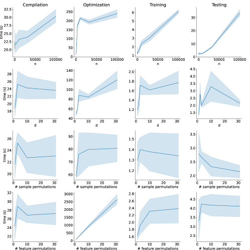
(b)

Figure 6: Computational study: computational time measured in elapsed seconds for a simple GMM example. Note that R-BP has the same computational complexity and only saves an indiscernible constant time factor.

Sensitivity analysis

For the sensitivity study, we consider the same simulated GMM data as in the computational study, and plot the results in Figure 7. As expected, we observe that the test NLL decreases in $n$, and in the number of permutations. It also decreases in the number of mixture components. One possible explanation for this is that, as noted by hahn2018recursive, R-BP can be interpreted as a mixture of $n$ normal distributions. The NLL decreases in $d$, as the mixture components are easier to distinguish in higher dimensional covariate spaces.

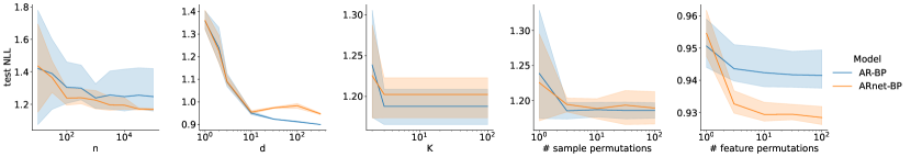
Figure 7: Sensitivity analyis: Average test NLL over 5 runs reported with standard error for a simple GMM example over a range of simulation and parameter settings.

Ablation study

Figure 7 shows the test NLL of ARnet-BP and AR-BP for the above GMM example, as a function of the number of sample permutations, and number of feature permutations. We see that averaging over multiple permutations is crucial to the performance of AR-BP. In Table LABEL:tab:smalluci_ablation, we also show results on the small UCI datasets for:

• a different choice of covariance function, namely a rational quadratic covariance function, defined by $k(x,x_{i})=\left(1+\frac{||x-x_{i}||^{2}_{2}}{2\gamma\ell^{2}}\right)^{-\gamma}$, where $\ell,\gamma>0$ and

• a different choice of initial distribution, namely a uniform distribution (unif).

Table 4: Average NLL with standard error over five runs on five UCI data sets of small-to-moderate size

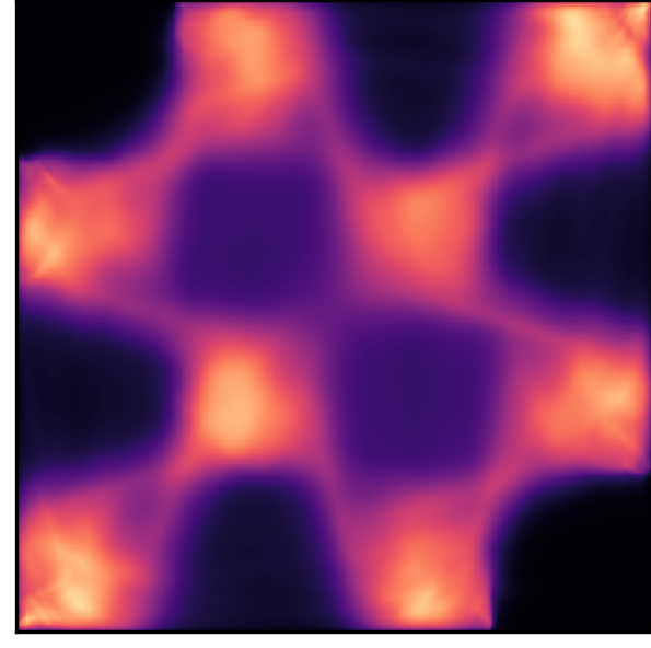
(e)

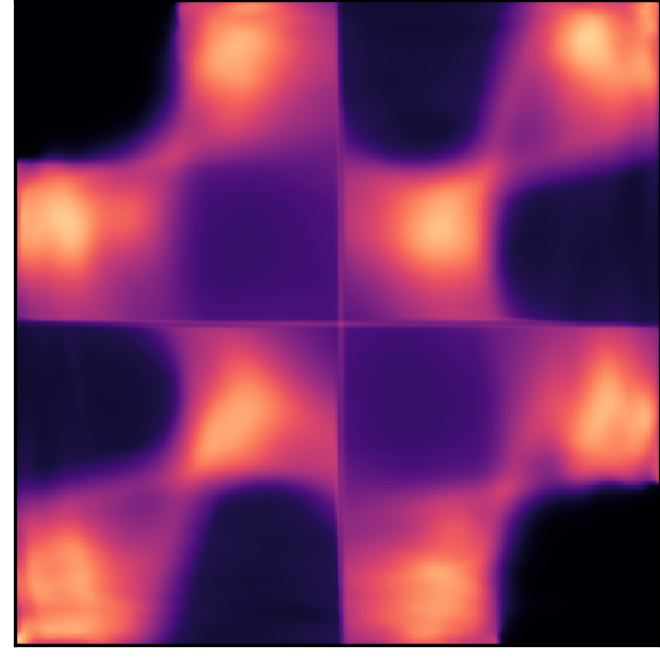
(f)

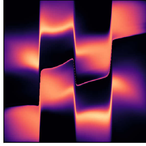
(g)

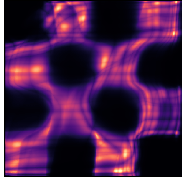
(h)

Figure 8: Scatter plot and density estimates of 60,000 observations sampled from a chessboard data distribution. Test log likelihoods are R-BP: $2.25_{\pm 0.0}$, R_d-BP : $2.19_{\pm 0.0}$, AR-BP: $2.21_{\pm 0.0}$, AR_d-BP: $2.10_{\pm 0.0}$, ARnet BP : $2.19_{\pm 0.0}$, MAF : $2.09_{\pm 0.0}$, RQ-NSF : $2.05_{\pm 0.0}$.

Table 6: Image datasets: average test NLL over five runs displayed with standard error

	DIGITS	MNIST
MAF	$\bm{-8.76_{\pm 0.10}}$	${-7.14_{\pm 0.48}}$
RQ-NSF	${-6.17_{\pm 0.13}}$	${-8.49_{\pm 0.03}}$
R-BP	${-8.80_{\pm 0.00}}$	${-9.04_{\pm 0.07}}$
Rd-BP	${-7.46_{\pm 0.12}}$	${-7.73_{\pm 0.07}}$
AR-BP	${-8.66_{\pm 0.03}}$	$-{7.31_{\pm 42.54}}$
ARd-BP	${-7.46_{\pm 0.18}}$	$-{8.32_{\pm 61.92}}$
ARnet-BP	${-7.72_{\pm 0.28}}$	$\bm{-9.20_{\pm 0.10}}$

Toy examples

Figure 4 shows density estimates for the introductory example of the checkerboard distribution in a large data regime. We observe that neural-network-based methods outperform the AR-BP alternatives. Nevertheless, AR-BP performs better than the baseline R-BP. An illustration of this behaviour on another toy example is also given in Figure 9. Figure 4 shows density estimates from AR-BP on a number of complex distributions.

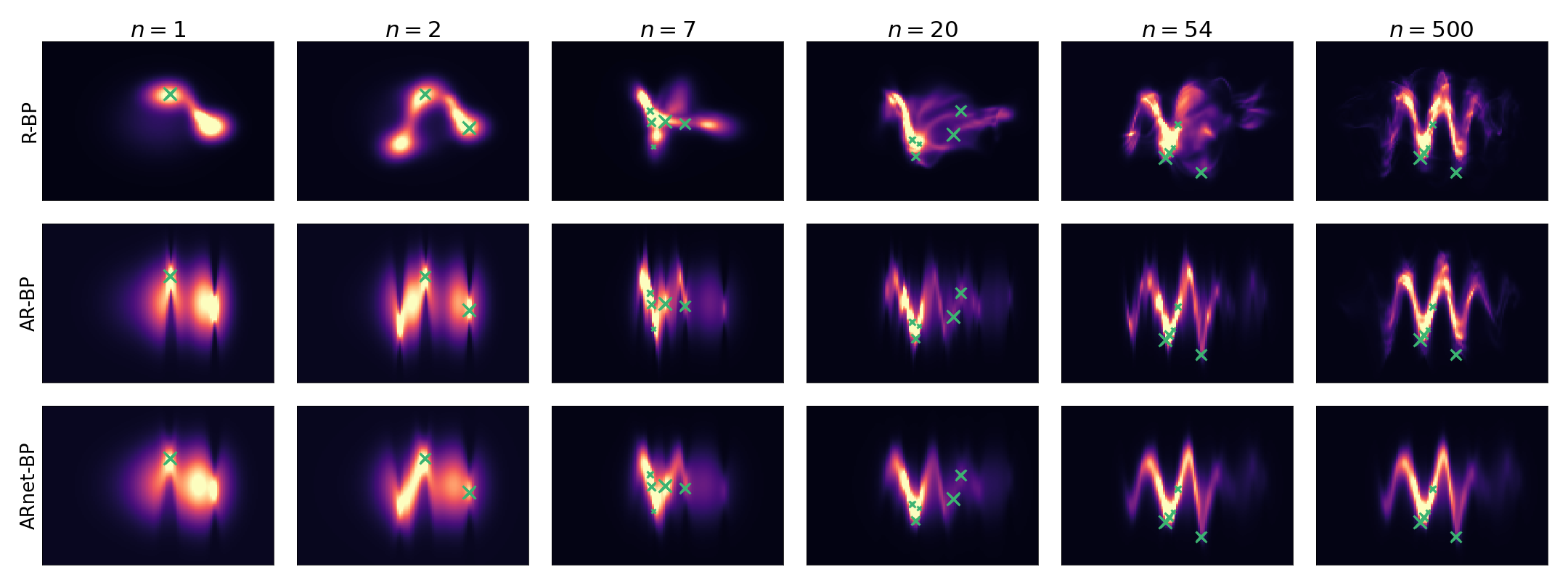
Figure 9: Illustration of the importance of an autoregressive kernel. We trained the models on 500 data points sampled according to a sine wave distribution (given in Figure 4). We visualise the predictive density after observing a different number, $n$, of observations, highlighting the last five points with . We observe that for highly non-linear relationships between $x^{1}$ and $x^{2}$, the optimal bandwidth of R-BP is quite high ($\rho=0.93$) which results in strong overfitting. Even when we choose $\rho_{0}=0.93$ for AR-BP and ARnet-BP, we observe that these models learn the true data distribution with fewer samples than R-BP does.

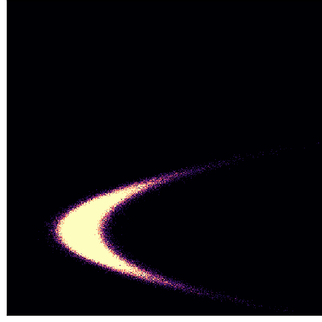
(a)

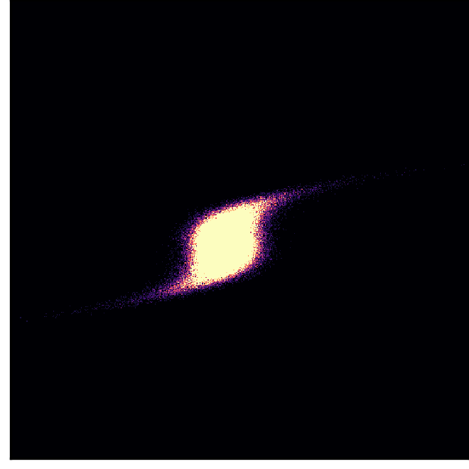
(b)

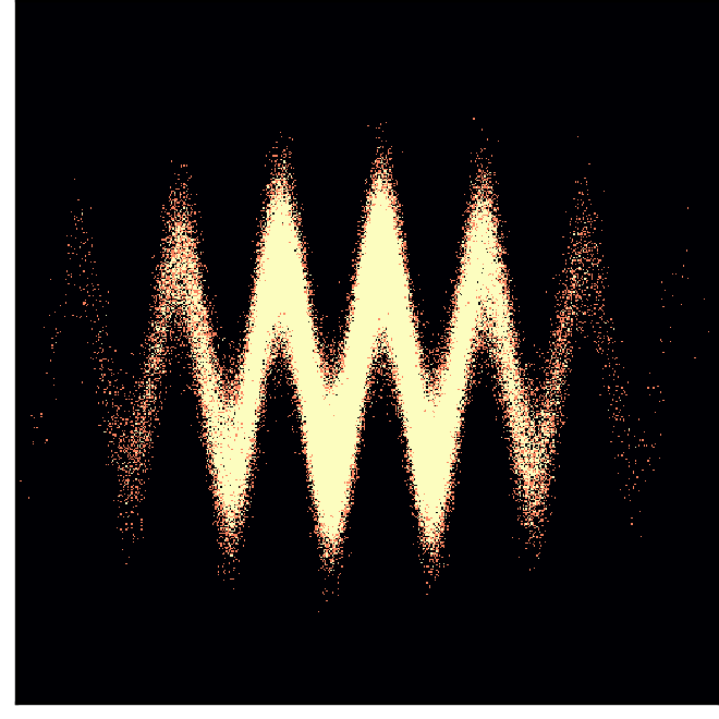
(c)

(d)

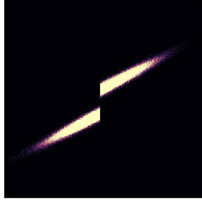
(e)

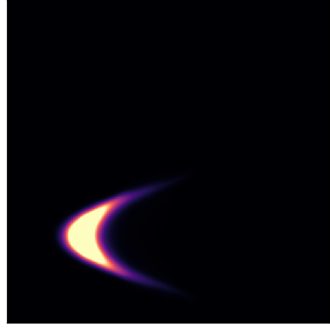
(f)

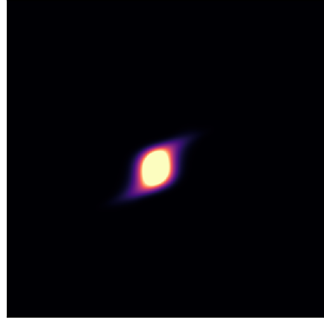
(g)

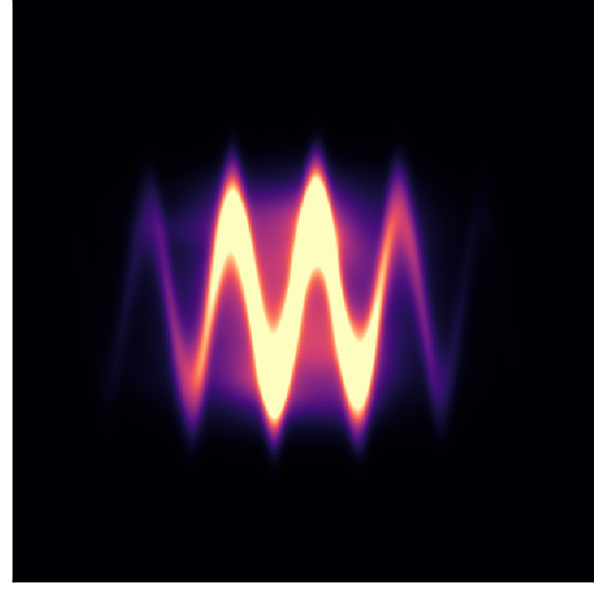
(h)

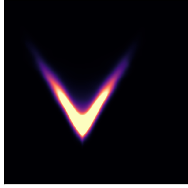
(i)

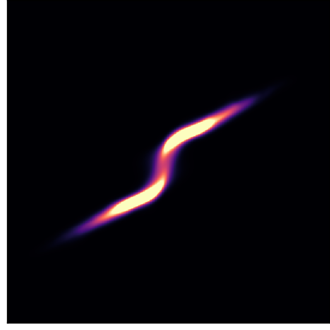
(j)

Figure 10: Scatter plots of 60,000 samples from different data distributions in the first row, and corresponding autoregressive predictive density estimates in the second row.