Supernova Dust Evolution Probed by Deep-sea ${}^{60}{\rm Fe}$ Time History

Abstract

There is a wealth of data on live, undecayed ${}^{60}{\rm Fe}$ ($t_{1/2}=2.6\ \rm Myr$) in deep-sea deposits, the lunar regolith, cosmic rays, and Antarctic snow, which is interpreted as originating from the recent explosions of at least two near-Earth supernovae. We use the ${}^{60}{\rm Fe}$ profiles in deep-sea sediments to estimate the timescale of supernova debris deposition beginning $\sim 3$ Myr ago. The available data admits a variety of different profile functions, but in all cases the best-fit ${}^{60}{\rm Fe}$ pulse durations are $>1.6$ Myr when all the data is combined. This timescale far exceeds the $\lesssim 0.1$ Myr pulse that would be expected if ${}^{60}{\rm Fe}$ was entrained in the supernova blast wave plasma. We interpret the long signal duration as evidence that ${}^{60}{\rm Fe}$ arrives in the form of supernova dust, whose dynamics are separate from but coupled to the evolution of the blast plasma. In this framework, the $>1.6$ Myr is that for dust stopping due to drag forces. This scenario is consistent with the simulations in Fry et al. (2020), where the dust is magnetically trapped in supernova remnants and thereby confined around regions of the remnant dominated by supernova ejects, where magnetic fields are low. This picture fits naturally with models of cosmic-ray injection of refractory elements as sputtered supernova dust grains and implies that the recent ${}^{60}{\rm Fe}$ detections in cosmic rays complement the fragments of grains that survived to arrive on the Earth and Moon. Finally, we present possible tests for this scenario.
  
KCL-PH-TH/2022-27, CERN-TH-2022-084

1 Introduction

Ellis et al. (1996) suggested that deposits of live radioactive isotopes including ${}^{60}{\rm Fe}$ could be a telltale sign for a recent near-Earth supernova explosion. Around the same time, Korschinek et al. (1996) proposed that the high sensitivity of accelerator mass spectrometry (AMS) could reach the levels needed to see a supernova signal. AMS has subsequently enabled widespread detections of live, i.e., undecayed, radioactive ${}^{60}{\rm Fe}$ in deep-sea samples from around the world  (Knie et al., 1999, 2004; Fitoussi et al., 2008; Ludwig et al., 2016; Wallner et al., 2016, 2021), which provide compelling evidence that radioisotopes from an astrophysical event reached Earth $\sim 3$ Myr ago (Mya). In addition, ${}^{60}{\rm Fe}$ has also been found in lunar samples (Fimiani et al., 2016), in cosmic rays (Binns et al., 2016), in Antarctic snow (Koll et al., 2019), and in a deep-sea ferromanganese (FeMn) crust from 6 to 7 Mya (Wallner et al., 2021). These signals far exceed known terrestrial and meteoritic backgrounds. The half-life of ${}^{60}{\rm Fe}$ $t_{1/2}=2.60\pm 0.05\ \rm Myr$ (Rugel et al., 2009; Wallner et al., 2015; Ostdiek et al., 2017) is much less than the age of the Earth, which implies that the astrophysical sources of these radioisotope deposits were relatively recent.

The explosion of at least one near-Earth supernova has been the general interpretation of the ${}^{60}{\rm Fe}$ data ever since the pioneering detections of Knie et al. (1999), with a distance estimated to be in the range of tens of parsecs (Fields & Ellis, 1999; Fields et al., 2008). Fry et al. (2015) expanded this analysis to consider all known or proposed astrophysical ${}^{60}{\rm Fe}$ sources, concluding that the ${}^{60}{\rm Fe}$ abundance and its implied distance rule out all but core-collapse supernovae and asymptotic giant branch (AGB) stars, as further discussed below.

The blast from a supernova at such a distance does not itself penetrate the heliosphere as far as the Earth’s orbit at 1 au (Fields et al., 2008; Miller & Fields, 2022), but supernova ejecta in the form of dust grains (Benítez et al., 2002) can reach the Earth and Moon (Athanassiadou & Fields, 2011; Fry et al., 2016). Iron is one of the most refractory elements, i.e., it has a high condensation temperature and readily forms dust, and ${}^{60}{\rm Fe}$ would be delivered in whatever iron-bearing dust particles survive the journey to the solar system. Fry et al. (2016) used the ${}^{60}{\rm Fe}$ flux to infer the distance to the supernova, finding $D_{\rm SN}\sim 30-150\ \rm pc$. The uncertainty is large, but encouragingly, this is precisely the plausible astrophysical range, neither so close as to cause a mass extinction, nor so far that the supernova material cannot reach us. Fry et al. (2016) also showed that the flux from the supernova blast, i.e., the gas, declines from an initial peak, corresponding to the passage of the dense supernova shell. At the distances implied by the strength of the ${}^{60}{\rm Fe}$ signal, the duration of the blast flux peak was found to be at most $\sim 0.1\ \rm Myr$.

Deep-sea sediments offer unprecedented time resolution of the ${}^{60}{\rm Fe}$ signal at the level of a few kiloyears (kyr), opening a new window on the possible nearby supernova(e). Fitoussi et al. (2008) pioneered this approach, searching for ${}^{60}{\rm Fe}$ in a sediment using AMS with lower sensitivity than is now available. They found no evidence for the short $\sim$ few kyr signal they expected, but showed that a potential signal emerged with time bins stretching to $\sim 1\ \rm Myr$. As we show below, subsequent high-sensitivity data from multiple sites and groups confirm that the width of the ${}^{60}{\rm Fe}$ deposition pulse arriving $\sim 3$ Myr ago exceeds $1\ \rm Myr$. This timescale is much longer than that of a blast from a single explosion (Fry et al., 2015), and understanding this long timescale for ${}^{60}{\rm Fe}$ deposition is the goal of this paper.

In this paper, we present an analysis of the ${}^{60}{\rm Fe}$ flux history for the four well-measured deep-sea sediment cores, two from Ludwig et al. (2016) and two from Wallner et al. (2016). We develop a statistical methodology appropriate for the ${}^{60}{\rm Fe}$ data, which are dominated by counting statistics, and use this to fit the ${}^{60}{\rm Fe}$ flux for the different cores individually and in a global fit with a focus on the signal timescale. We compare a variety of simple fitting functions, and all show that the timescale must exceed 1 Myr. We also test the ability of the data to discriminate among different time histories, finding that this is not possible with current data.

We interpret the long ${}^{60}{\rm Fe}$ deposition timescale based on the assumption that the supernova dust is decoupled from the gas, with different dynamics, so that the dust particle density profile is different from the blast profile. Such decoupling was found by Fry et al. (2020) in a study of dust propagation in a supernova remnant. Here we extract the key physics of this process and present a model for the dust flux versus time, which we compare with the available data. We then discuss a number of consequences and tests of our model.

Our work builds on the insights and analysis of Ellison et al. (1997), who noted that supernova grains are charged, and that they decouple from the gas. These authors further proposed that grains are accelerated by the same diffusive shock acceleration processes that lead to cosmic-ray acceleration. Indeed, they proposed that the sputtered atoms of the accelerated dust are injected as cosmic rays, and that this population is responsible for the observed enhancement of refractory elements in cosmic rays (Meyer et al., 1997). Giacalone & Jokipii (2009) have performed simulations of dust in the presence of supernova shocks, and found that grains initially at rest were accelerated to more than 10 times the shock speed. Our model elaborates this picture: as described below in §4, we propose that the ${}^{60}{\rm Fe}$ deposits on the Earth and Moon arise from the portions of iron-bearing supernova dust that have survived propagation to the Earth, while the ${}^{60}{\rm Fe}$ detected in cosmic rays (Binns et al., 2016) represents the portion that was sputtered along the way.

This paper is structured as follows. We discuss the time-resolved ${}^{60}{\rm Fe}$ sediment data in §2. We perform fits to the data in §3, deriving constraints in the ${}^{60}{\rm Fe}$ deposition timescale and finding it to be $>1\ \rm Myr$. We show in §4 that this long timescale is consistent with a picture of charged supernova dust propagation in a magnetized interstellar medium (ISM). We propose tests of this model in §5. We summarize our conclusions in §6.

2 Time-resolved Measurements of ${}^{60}{\rm Fe}$ Deposition on Earth

The evidence for ${}^{60}{\rm Fe}$ deposition on Earth comes mainly from deep-sea deposits, namely ferromanganese (FeMn) crusts and nodules, as well as sediment cores. The FeMn crusts and nodules exhibit relatively slow growth, $\sim$ few mm Myr^-1, which implies less dilution of the small extraterrestrial signal and facilitated the first detections (Knie et al., 1999). However, the slow growth rate makes it more difficult to obtain good time resolution. On the other hand, the growth (i.e., sedimentation) rates of deep-sea sediments are typically about a factor of 1000 faster, namely $\sim$ few mm kyr^-1. This means that a larger sample and more processing are needed to find the signal, but it is also easier to obtain good time resolution.

The importance of the ${}^{60}{\rm Fe}$ signal width as an observable goes back at least to Feige (2014). She illustrated possible pulse shapes assuming a Gaussian form, emphasizing the trade-off between ability to resolve the width and dilution of the signal at its peak. When Fitoussi et al. (2008) performed the first sediment measurements with relatively low ${}^{60}{\rm Fe}$ sensitivity, their results were hampered by this trade-off, which led to small ${}^{60}{\rm Fe}$ counts spread over $\sim 1\ \rm Myr$. In addition, they adopted time bins of about 10 kyr, anticipating a short signal consistent with a Sedov-Taylor blast; this further diluted the signal. By attaining improved sensitivity and adopting larger time bins, Ludwig et al. (2016) and Wallner et al. (2016) later unambiguously resolved the signal; Feige et al. (2018) performed an initial Gaussian fit to the binned Wallner et al. (2016) sediment data. The time is ripe for a detailed joint analysis of these results, as presented in this paper.

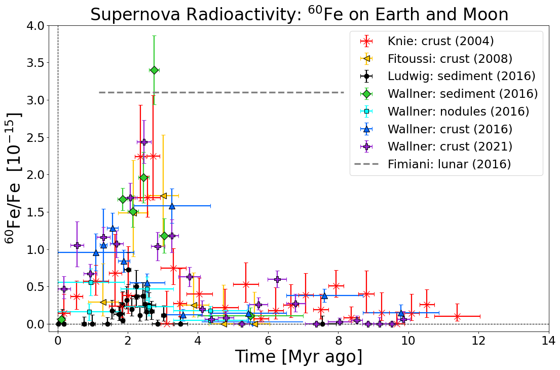
Figure 1: Terrestrial and lunar detections of ⁶⁰Fe. The ⁶⁰Fe/Fe fractions found in deep-sea sediments, FeMn crusts, and Apollo lunar samples; the data are not decay corrected for ${}^{60}{\rm Fe}$; however the Knie et al. (2004) and Fitoussi et al. (2008) times have been updated to take account of the latest ${}^{10}{\rm Be}$ half-life ($t_{1/2}=1.387\pm 0.012$ Myr; (Korschinek et al., 2010)). None of the data are background corrected. All of the data with time resolution show a signal around $\sim 2-3$ Mya. The amplitude differences may reflect variations in iron uptake, latitude variations in iron deposition, and/or differences in sampling technique. Note the appearance of a second distinct peak around $\sim 6-7$ Mya in the Wallner et al. (2021) data.

2.1 Measurements of Pulses around 3 and 7 Myr Ago

The presence of deep-sea pulses of live ${}^{60}{\rm Fe}$ is now compelling, providing strong evidence for recent nearby supernovae. Figure 1 compiles the published ${}^{60}{\rm Fe}$ data. The figure shows the detected ${}^{60}{\rm Fe}$/Fe isotope fraction versus time, categorized by both sample type and research group; none of the data have been background corrected. The data show two distinct peaks, with all groups agreeing on a ${}^{60}{\rm Fe}$ peak around $2-3$ Mya and the Wallner et al. (2016, 2021) data indicating another peak around $6-7$ Mya. Note that this peak at 7 Mya only appears clearly in the Wallner et al. (2021) data, whose ${}^{60}{\rm Fe}$ machine background has finally been lowered enough to show a distinct peak; the background in earlier efforts obscured the signal. Not included in this figure are the recent ${}^{60}{\rm Fe}$ flux measurements by Koll et al. (2019) and Wallner et al. (2020), as they cover collectively only the last 30 kyr and would not be visibly distinguishable from the origin (see §2.2). The Fimiani et al. (2016) lunar data are included for completeness only: due to micrometeorite gardening effects on the lunar regolith, the data cannot be time resolved to better than $\sim 8\ \rm Myr$. Because of this time range, the lunar data include the signals due to all supernovae in the last 10 Myr; however, due to the half-life of ${}^{60}{\rm Fe}$, the contribution of ${}^{60}{\rm Fe}$ from the pulse at 7 Mya is only around 10%.

When comparing the ${}^{60}{\rm Fe}$/Fe measurements, one should bear in mind that the geographical distribution of ${}^{60}{\rm Fe}$ may not be uniform, and that the uptake, $U$, of ${}^{60}{\rm Fe}$ varies in different materials. Specifically, it was shown in Fry et al. (2016) that the transport of ${}^{60}{\rm Fe}$ through the atmosphere should not be isotropic, but rather would favor middle latitudes $\sim 60^{\circ}$, with minima at the equator and poles (see also Dhomse et al., 2013), yielding a factor of $\sim 3$ in the global difference. This may explain some of the large difference between the flux values reported by Wallner et al. (2016) taken at $\sim 38^{\circ}\rm S$ versus the those in the data of Ludwig et al. (2016) taken at $3^{\circ}\rm S$. In addition, ocean currents may cause variations with longitude in the deposition of ${}^{60}{\rm Fe}$ in FeMn crusts and deep-sea sediments at similar latitudes. Differences in analytical technique and sample processing can also affect the final result. We note finally that the uptake is expected to be 100% for sediments and snow, whereas the uptake in FeMn crusts is subject to considerable uncertainty and debate, and may vary depending on location and local conditions (Bishop & Egli, 2011).

In this paper, we focus on the sediment data when estimating the timescale of astrophysical ${}^{60}{\rm Fe}$ deposition, in view of the availability of multiple samples with time resolution from deep-sea sediments (Ludwig et al., 2016; Wallner et al., 2016). We note that the Wallner et al. (2021) ${}^{60}{\rm Fe}$ data from the FeMn crust also has excellent time resolution compared to earlier studies. However, analysis of the deposition timescale requires strict accounting for geophysical processes that might disturb the signal, and this is more straightforward when the data are from the same sample type. By focusing on the unbinned sediment data, we can control most of the variables between the two data sets and therefore make fair comparisons. It should be noted that this approach by necessity deals with very small-count statistics; we address the issue in §3.1. We look forward to additional measurements of the 7 Myr peak, ideally in sediments, to allow for a similar analysis of that event.

2.2 Recent ${}^{60}{\rm Fe}$ infall

Koll et al. (2019) and Wallner et al. (2020) have shown independently that there is recent and ongoing infall of extrasolar ${}^{60}{\rm Fe}$ onto Earth. Koll et al. (2019) detected an ${}^{60}{\rm Fe}$ signal in Antarctic snow deposited over the last 20 yr and use isotopic ratios to show it is not from meteoritic material and must therefore be extrasolar. They suggest that the signal is due to the solar system passing through the Local Interstellar Cloud (a nearby higher-density region of the Local Bubble). Wallner et al. (2020) also detected a fairly steady ${}^{60}{\rm Fe}$ signal in deep-sea sediments over the last 33 kyr, in line with the Koll et al. (2019) detection. However, they do not see the sharp increase in the ${}^{60}{\rm Fe}$ signal that would be expected from the solar system entering the Local Interstellar Cloud. There are other possibilities for the persistent ${}^{60}{\rm Fe}$ flux, including continued delivery of dust following the most recent pulse $\sim 3$ Mya, or flux from the Earth’s motion through the local ISM. Further analysis of ${}^{60}{\rm Fe}$ in FeMn crusts and deep-sea sediments focused on the age range from 40 Kya to 1 Mya could add significant insight into the origin of the observed recent infall.

That said, the main purpose of this paper is to characterize the peaks that are clearly evident in the data, and we do not attempt to fit the low-level ${}^{60}{\rm Fe}$ flux outside the peaks.

3 Supernova Dust Deposition Timescale from ${}^{60}{\rm Fe}$ in Deep-sea Sediments

Ocean sediments are the most suitable tracers for timescale analysis due to their rapid growth rate $\sim$ few mm kyr^-1, which is a factor $\sim 10^{3}$ faster than that of the ferromanganese crusts. This rapid growth allows the sediment column to be sampled more finely, leading to much better time resolution, but at the cost of a lower ${}^{60}{\rm Fe}$ concentration. We study the sediment data of Wallner et al. (2016) and Ludwig et al. (2016), which were taken from different ocean drilling program cores and analyzed independently. Wallner et al. (2016) made measurements in four cores, of which two probe a very limited time range, leaving two cores (4521 and 4953) with sufficient data for our analysis. The two cores (848 and 851) studied by Ludwig et al. (2016) are both sufficiently well sampled for our purposes. Unfortunately, the pioneering Fitoussi et al. (2008) data did not have sufficient sensitivity for a well-resolved time series; they still provide useful consistency checks, but we do not use them for our full timescale study.

Both Wallner et al. (2016) and Ludwig et al. (2016) used AMS measurements of ${}^{60}{\rm Fe}$ atoms in the samples, from which ${}^{60}{\rm Fe}$/Fe isotope fractions are derived, as well as the ${}^{60}{\rm Fe}$ flux and its time-integrated fluence. Additionally, both groups studied blank samples to infer that their background is negligible, and therefore all of the ${}^{60}{\rm Fe}$ counts are significant.

Table 1: Summary of Timescales of Nonzero Counts in Deep-sea Drill Cores

Core	$t_{\rm last}$	$t_{\rm first}$	$\delta t=t_{\rm first}-t_{\rm last}$
Name	(Mya)	(Mya)	(Myr)
Ludwig 848	1.528	2.604	1.076
Ludwig 851	1.735	3.045	1.310
Wallner 4521	1.78	2.57	0.79
Wallner 4953	1.71	3.18	1.47
All Cores	1.528	3.18	1.65

Before performing our fits, it is useful to note that the raw data give useful information about the signal width. For each core, there is a distribution of nonzero ${}^{60}{\rm Fe}$ counts. The interval $\delta t=t_{\rm first}-t_{\rm last}$ between the time $t_{\rm first}$ of the first nonzero count and the time $t_{\rm last}$ of the last nonzero count thus gives a minimum time span for each core. This assumes that background effects are negligible. These results are summarized in Table 1, where we see that the signal durations in the individual cores span $\delta t=0.79$ to 1.47 Myr. It is important to note that the Ludwig cores have multiple measurements with zero counts before and after the ranges of their nonzero measured counts; this is not the case for the Wallner data. Thus the Ludwig results in Table 1 represent an estimate of their signal duration; though Poisson fluctuations or flux beneath their sensitivity could lead to a longer signal. For the Wallner data, there are no leading and trailing zero counts, and so the results in Table 1 are certainly a lower limit to the duration in the cores they measured.

If we further assume there are no systematic differences in absolute timing, then all of the cores together probe the range of the signal. Then the global minimum time span is the interval between overall first and last nonzero counts among all the cores. Globally, the ${}^{60}{\rm Fe}$ detections in sediments span 1.65 Myr. We already see that the signals are quite long compared to the Sedov timescale $\lesssim 0.1$ Myr. As we now turn to fits, we will find that these characteristic timescales set lower limits to our results.

3.1 Analysis of the ${}^{60}{\rm Fe}$ timescale

The purpose of this work is to determine the deposition or “raindown” time onto Earth of ${}^{60}{\rm Fe}$ during the recent pulse $\sim 3$ Mya, and to interpret what this timescale implies about the propagation of supernova-produced material inside the remnant. In order to perform this analysis, we fit the observed ${}^{60}{\rm Fe}$ signal with a number of 3-parameter pulse shapes to see which one best described the data, while assuming the errors are dominated by Poisson counting statistics. These shapes included a Gaussian, sawtooth, reverse sawtooth (for comparison, despite our doubt that this is a physically plausible profile), and a symmetric triangle; expressions appear in Appendix A. We also performed one 4-parameter fit with an asymmetric triangle to see if there is a preferred slant to the data.

The general shape of the ${}^{60}{\rm Fe}$ data is of particular interest, because the sharpness and slant of the shape can provide insight into the astrophysics of the deposition of the ${}^{60}{\rm Fe}$ and its path within the supernova remnant. Predictions in the literature to date have assumed the ${}^{60}{\rm Fe}$ traces the gas phase of the blast. Under this assumption, Fry et al. (2015) showed that if the ${}^{60}{\rm Fe}$ is well mixed in a Sedov blast, the signal appears discontinuously with the arrival of the forward shock, and decreases thereafter from this maximum. Chaikin et al. (2022) included the effects of incomplete mixing of ${}^{60}{\rm Fe}$ in the remnant gas, and also allowed for effects of the Earth’s motion. They too found that the ${}^{60}{\rm Fe}$ pulse begins abruptly and is concentrated in a pulse, but found that the signal can linger thereafter. Thus, these models would favor the discontinuous profiles we have considered — the sawtooth form, or a cut exponential. As we will see, there are other possibilities if the ${}^{60}{\rm Fe}$ is in dust that is decoupled from the gas, so we have chosen a suite of different fitting functions to allow for a range of possible ${}^{60}{\rm Fe}$ flux histories.

In the published versions of their work, both Wallner et al. (2016) and Ludwig et al. (2016) bin their data, which serves to demonstrate the strength and overall peak of the signal. For the purposes of this analysis, we use the original, unbinned data, as it removes extraneous smoothing, and we are specifically interested in fitting the unbinned shape. The unbinned ${}^{60}{\rm Fe}$ data can be found in Table S.4 of Wallner et al. (2016) and in Tables A.1 and A.2 of Ludwig (2015). Both Wallner et al. (2016) and Ludwig et al. (2016) assume zero background for their analyses. As mentioned above, recent works by Wallner et al. (2020) and Koll et al. (2019) have found a nonzero ${}^{60}{\rm Fe}$ background today. This minor discrepancy is discussed in more detail in §2.2. For this work, we use the zero background estimate assumed by the original analyses.

In each sediment, AMS measures individual ${}^{60}{\rm Fe}$ atoms in each sediment segment corresponding to a time bin. The numbers of counts measured is small: in all of their sediments, Ludwig et al. (2016) detected a total of 89 atoms of ${}^{60}{\rm Fe}$, while Wallner et al. (2016) measured a total of 288 atoms. The $n_{i}$ number of ${}^{60}{\rm Fe}$ counts in each time bin $i$ is therefore also small, with $n_{i}\leq 23$ and often $n_{i}<10$. As a result, the Poisson errors in the counts dominate the uncertainties in the resulting ${}^{60}{\rm Fe}$ flux. We therefore tailor our analysis to identify the dependence on count numbers $n_{i}$ and to treat these Poisson errors appropriately.

The observed ${}^{60}{\rm Fe}$ flux values $\Phi_{60}$ (the deposition into the material) are computed by combining the measured ${}^{60}{\rm Fe}$ counts with properties of the sediment, as follows. For each time $t_{i}$, a number $n_{i}$ of ${}^{60}{\rm Fe}$ atoms are measured. From this, the observed ${}^{60}{\rm Fe}$/Fe ratio is determined:

$$\left(\frac{\mbox{${}^{60}{\rm Fe}$}}{{\rm Fe}}\right)_{i}=s_{i}\ n_{i}\,,$$ (1)

where the scaling $s_{i}$ is due to variations in efficiency and other factors, and unique for each measurement. We infer the scalings from the reported $n_{i}$ and $(\mbox{${}^{60}{\rm Fe}$}/\mathrm{Fe})_{i}$. In the cases of null measurements, we follow the same procedure as both experimental groups, using the Feldman & Cousins (1998) prescription for calculating 69.29% CL limits based on $n_{i}=0$ counts, and a background $b=0$. This gives an effective limit $n_{i}^{\rm eff}<1.29$, which we use to infer the scaling $s_{i}$ for these measurements.

We use the following equations to correct the data for decays:

$$\left(\frac{\mbox{${}^{60}{\rm Fe}$}}{\rm Fe}\right)_{\rm c} =\left(\frac{\mbox{${}^{60}{\rm Fe}$}}{\rm Fe}\right)\,\exp{\left[\frac{t_{i}}{\tau}\right]}\,,$$ (2)

$$\sigma_{60_{\rm c}} =\sqrt{\exp{\left[\frac{2\,t_{i}}{\tau}\right]}\sigma_{60}^{2}+\left(\dfrac{\mbox{${}^{60}{\rm Fe}$}}{\mathrm{Fe}}\ \dfrac{1}{\tau}\right)^{2}\exp{\left[\frac{2\,t_{i}}{\tau}\right]}\sigma_{i}^{2}}\,.$$ (3)

Here and throughout, the subscript “${\rm c}$” indicates that the quantity is decay corrected, $t_{i}$ is the observed time with uncertainty $\sigma_{i}$, $\tau$ is the mean lifetime of ${}^{60}{\rm Fe}$, and $\sigma_{60_{\rm c}}$ is the uncertainty in the decay-corrected ${}^{60}{\rm Fe}$/Fe ratio. To calculate the ${}^{60}{\rm Fe}$ flux, we use

$$\Phi_{\rm 60c} =n_{\rm 60c}\dot{h}=\left(\frac{\mbox{${}^{60}{\rm Fe}$}}{\rm Fe}\right)_{\rm c}n_{\rm Fe}\,\dot{h}=\frac{X_{\rm Fe}}{A_{\rm Fe}m_{\rm u}}\left(\frac{\mbox{${}^{60}{\rm Fe}$}}{\rm Fe}\right)_{\rm c}\,\rho\,\dot{h}$$ (4)

$$=c_{\mathrm{Fe}}\,\left(\frac{\mbox{${}^{60}{\rm Fe}$}}{\rm Fe}\right)_{\rm c}\,\rho\,\dot{h}\,,$$ (5)

$$\sigma_{\Phi} =c_{\mathrm{Fe}}\,\sigma_{60c}\,\rho\,\dot{h}\,.$$ (6)

In eq. (4), $\Phi$ is the flux of ${}^{60}{\rm Fe}$, and $n_{60}$ is the ${}^{60}{\rm Fe}$ number density. The sediment mass density is $\rho$, $\dot{h}$ is the sedimentation rate, and $X_{\rm Fe}=\rho_{\rm Fe}/\rho$ is the mass fraction of iron in the sediment. The factor $c_{\mathrm{Fe}}=X_{\rm Fe}/A_{\rm Fe}m_{\rm u}$ measures the concentration of iron in the sediment in atoms per unit mass, with $A_{\rm Fe}$ as the mean molecular weight of iron and $m_{\rm u}$ as the atomic mass unit.

Due to the format of the data provided in the relevant papers, the conversion of the ${}^{60}{\rm Fe}$/Fe ratio into a flux was by necessity different for the two groups. Wallner et al. (2016) calculated the flux in their Table S.4, following the formula in Eq. (4), and we use those numbers directly. However, Ludwig et al. (2016) used a protocol in their chemical sample treatment (citrate-bicarbonate-dithionite, hereafter CBD) that effectively separates larger iron-bearing grains from smaller grains, which they argue should arise from fossilized magnetotatic bacteria. Their AMS measurements thus give a $(\mbox{${}^{60}{\rm Fe}$}/{\rm Fe})_{\rm CBD}$ ratio for this material, and thus their scaling $c_{\rm Fe}$ of iron per mass in the bulk unprocessed sediment includes a factor $Y_{\rm CBD}$ for the fraction of iron selected by the CBD process. This implicitly assumes that the Fe-bearing material excluded from the CBD protocol does not contain ${}^{60}{\rm Fe}$. For the flux calculation in Eq. (4), the unbinned ${}^{60}{\rm Fe}$/Fe ratio and extracted iron are from Tables A.1 and A.2 in Ludwig (2015) (the binned versions of which appear in Ludwig et al. (2016)), the sediment density is taken from Table 6.3 in Ludwig (2015), and the sedimentation rate is from Figure 1 in Ludwig et al. (2016).

Combining eqs. (1) and (4), we arrive at the relationship between the flux and ${}^{60}{\rm Fe}$ counts. For time $t_{i}$, we have

$$\Phi_{60,c}(t_{i})=\frac{X_{\rm Fe}}{A_{i}m_{\rm u}}\rho\dot{h}\ e^{t_{i}/\tau}\ s_{i}\ n_{i}\ \equiv\ \varphi_{i}\ n_{i}\,.$$ (7)

Given the counts $n_{i}$ and the other observables, eq. (7) allows us to determine the flux scalings $\varphi_{i}$. As we now see, these allow us to compare the observed fluxes to model predictions.

Our goal is to fit the observed flux data with several simple models that capture different qualitative trends one might expect in the ${}^{60}{\rm Fe}$ flux versus time, $\Phi_{\rm model}$. The flux profile versus time is described by a set of parameters $\vec{\theta}$, so that we have $\Phi(t;\vec{\theta})$. In designing our fitting procedure, we are guided by the fact that the uncertainties in the ${}^{60}{\rm Fe}$ flux are dominated by the Poisson errors in the ${}^{60}{\rm Fe}$ counts, which is the case for both the Wallner et al. (2016) and Ludwig et al. (2016) data sets. We have designed our fitting procedure to accommodate this situation, closely following the approach laid out by Cash (1979), originally for determining X-ray fluxes from photon count measurements dominated by Poisson uncertainties.

Our analysis requires that at each time $t_{i}$ we specify the expected number $\mu_{i}$ of events, based on the model flux. To do this, we evaluate $\Phi_{\rm model}(t_{i};\vec{\theta})$ and then infer $\mu_{i}(\vec{\theta})=\Phi_{\rm model}(t_{i};\vec{\theta})/\varphi_{i}$, using the the scaling $\varphi_{i}$ found in eq. (7). For each measured number of counts $n_{i}$ the fit function with parameters $\vec{\theta}$ gives an expected value $\mu_{i}(\vec{\theta})$.

We now construct a Poisson-based likelihood for the fit given the data. For time $t_{i}$, the likelihood for the fit given the data is just the Poisson probability ${\cal L}_{i}(n_{i}|\vec{\theta})=P(n_{i}|\mu_{i})$, where $P(n|\mu)=\mu^{n}e^{\mu}/n!$ is the Poisson probability of $n$ counts given a mean $\mu$. The total probability for the fit given all of the data is just the product of the likelihoods at each time:

$$\mathcal{L}(\mbox{data}|\vec{\theta})=\prod_{i}{\cal L}_{i}(n_{i}|\mu_{i})=\prod_{i}\frac{\mu_{i}^{n_{i}}}{n_{i}!}e^{-\mu_{i}}$$ (8)

where the fit parameter dependence is through $\mu_{i}(\vec{\theta})$. The negative of the logarithm of the total likelihood in eq. (8) is

$$C(\vec{\theta})=-\ln\mathcal{L}(\mbox{data}|\vec{\theta})=-\sum_{i}\left(\mu_{i}-n_{i}\ln\mu_{i}\right)+\mbox{const}\,.$$ (9)

Here the constant sums terms with $\ln n_{i}$ dependencies that do not depend on the fit parameters $\vec{\theta}$, which means that it does not affect the relative likelihoods of different parameter choices, so we follow the usual practice and neglect it. The function $C$ thus depends on the data and the fit parameters, and determines the goodness of fit in a way closely analogous to the role of a $\chi^{2}$ for data that is continuous rather than discrete.

For a given dataset and fitting function $\Phi_{\rm model}(t;\vec{\theta})$, eq. (9) will give different values to $C$ for different choices of the parameters $\vec{\theta}$. The likelihood is maximized at the minimum value for $C$, which we call $C_{\rm min}$, and which we will use to assess goodness of fit. The parameters $\vec{\theta}$ giving $C_{\rm{min}}$ are the best-fit values. We use Monte Carlo methods to explore the parameter space, find the best-fit parameters, and characterize their uncertainties.

We note that the physical picture of supernova radioisotope deposition could include an abrupt onset to the flux. This could occur if ${}^{60}{\rm Fe}$ is entrained in a blast wave, so that the onset of the ${}^{60}{\rm Fe}$ coincides with the forward shock’s arrival at the solar system. To allow for this, we consider some fitting functions where the flux has an abrupt onset and/or halt. In these cases, there are times before or after the blast passage, for which there is no signal: $\mu_{i}=0$, which means that the expected number of counts must be zero. If the measured number of counts is nonzero for these times, then the Poisson probability is zero ($C\rightarrow-\infty$) and this set of fit parameters is completely ruled out. In other words, our method automatically rejects the models (regions of parameter space) that predict no counts where some are observed. On the other hand, the converse is not true: if the fit has $\mu_{i}>0$, Poisson statistics allow for cases where $n_{i}=0$, albeit with a penalty.

Each of the four sediment cores was fitted separately, as each core is a separate time column, and in many cases, data points from different cores lie on the same time slice, which creates difficulties with Poisson statistics. We were also interested in examining any differences we could find in the pulse arrival time and the peak pulse time, to see if there were differences in the timing calibration between the different sediments. In order to ensure a universal resolution for all the pulse shapes, we enforced the same initial parameters across all of the 3-parameter fits (similar values were used for the 4-parameter fit, although it is not statistically comparable).

To test our methodology, we generated simulated data points, drawn from a predetermined flux history $\Phi_{\rm true}(t)$. We randomly chose sample times $t_{i}$, and drew counts $n_{i}$ from a Poisson distribution appropriate for our flux history. We found that our method generally performed well: the best-fit parameters were close to the parameters of the known input $\Phi_{\rm true}$. However, we did find that the accuracy and precision of the width and thus timescale parameter depends on the functional form and the time distributions of measurements. In particular, we found that a crucial factor is the number of measured points with zero counts before and after the bulk of the signal. The more leading and trailing null points, the better the width was determined. On the other hand, if there were only one or two null points on either side of the signal, the width was less well constrained, with the true width being at the low end of the range allowed by the fit. This is a manifestation of the physical effect that in noisy data with small mean numbers of counts, one or two bins with zero counts do not strongly constrain the fit; rather, many are needed to exclude the models that span wide timescales. We will see this behavior manifested in the fits below.

3.2 Results of Fits

To allow for a variety of possible ${}^{60}{\rm Fe}$ time histories, we fit the flux data with six possible 3-parameter shapes, chosen for mathematical simplicity and resemblance to physically motivated trends suggested in the literature. Their mathematical expressions are given in in Appendix A. Three of these give a signal that has a finite duration: (1) a symmetric triangle with equal duration linear rise and fall around a peak, (2) a sawtooth that begins abruptly at a peak and falls linearly to zero, (3) and a reverse sawtooth that rises linearly from zero to a peak, then drops to zero. We explored three additional profiles that allow comparison to traditional fits and explore a more gradual rise and fall that formally never goes to zero: (1) a Gaussian, (2) a Lorentzian, and (3) a cut exponential that starts at a peak and then drops exponentially.

The data for each sediment core were fit with each specific fit model. The results are summarized in Tables 2 and 3, but for brevity we plot results only for select cases. Figures 2–5 show results for all cores using the sawtooth fit, while Fig. 6 shows the results for the Ludwig 848 core using a Gaussian fit. Each fit figure shows the flux versus time data for a single core. The middle part of the figure plots the ${}^{60}{\rm Fe}$ flux (in $10^{4}\,\rm atoms\ cm^{-2}\ kyr^{-1}$) versus time (in Mya), including both detections and nondetections. Overlaid on top of these points is the best-fit curve, with the $C_{\rm{min}}$ statistic and the fit’s peak time ($t_{\rm{peak}}$), peak flux ($\Phi_{\rm{peak}}$), and width ($\sigma_{t}$) given in the upper left corner. The top three plots in each figure display two-dimensional projections of the three parameters of each fit model, exhibiting the contour confidence levels of $\Delta C$ = $C-C_{\rm min}$ corresponding to 1$\sigma$, 2$\sigma$, and 3$\sigma$ for a three-dimensional Gaussian; the bottom three plots show the marginalized likelihood for each parameter normalized so that the peak is at 1.

Figure 2: Sawtooth fits to the terrestrial ⁶⁰Fe flux of Ludwig et al. (2016) core 848. The flux is in units of $[10^{4}\ \rm atoms\ cm^{-2}\ kyr^{-1}]$ throughout. Upper plots: the confidence intervals as contours for the three fit parameters (peak time, signal width, and peak flux). Middle plot: the ${}^{60}{\rm Fe}$ flux vs. time, with the sawtooth best fit overlaid in red. The dark blue points show the calculated flux for the detected ${}^{60}{\rm Fe}$ counts, while the light blue points show the flux upper limits for the nondetections. Error bars in both flux and time are included, although the time errors can be smaller than the data point itself. In the upper left corner are listed the best-fit peak time, width, and peak flux values for the sawtooth fit, as well as the $C_{\mathrm{min}}$ parameter for the fit. Lower plots: the marginalized likelihood for each of the three parameters, with the best-fit value indicated by a red line.

Figure 3: Sawtooth fits to the terrestrial ⁶⁰Fe flux of Ludwig et al. (2016) core 851, as in Fig. 2.

Figure 4: Sawtooth fits to the terrestrial ⁶⁰Fe flux of Wallner et al. (2016) core 4521, as in Fig. 2.

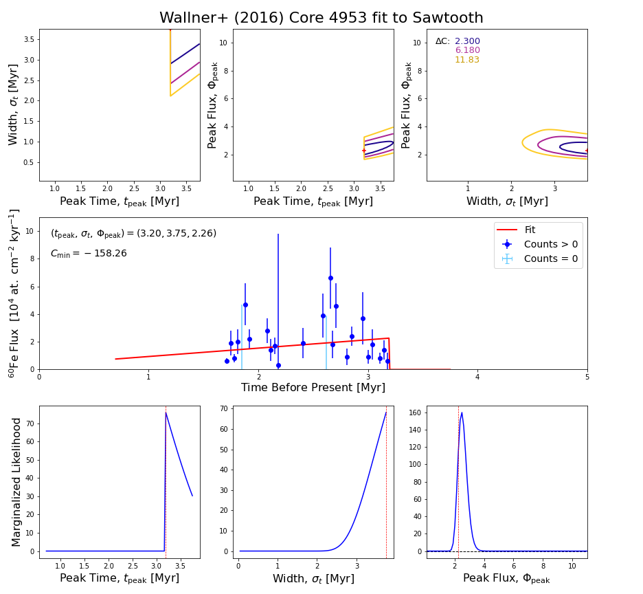
Figure 5: Sawtooth fits to the terrestrial ⁶⁰Fe flux of Wallner et al. (2016) core 4953, as in Fig. 2.

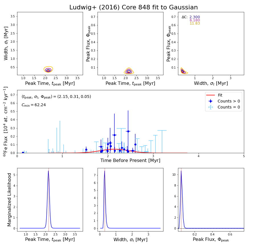
Figure 6: Gaussian fits to the terrestrial ⁶⁰Fe flux, Ludwig et al. (2016) core 848, as in Fig. 2. Shown here as an example of an alternative fit.

Figure 7: Best-fit curves for each 3-parameter fit for each core. The Ludwig fluxes have been multiplied by 10 for ease of comparison. Curves are plotted over the time domain for which there is data from at least one measurement.

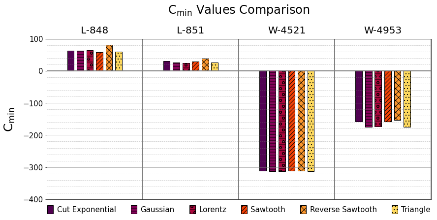
Figure 8: Assessing goodness of fit: 3-parameter fit $C_{\rm{min}}$ comparisons for each of the 6 fits per core. The lower (more negative) the $C_{\rm{min}}$ value, the better the fit. Note that, while the fits can be compared with each other for each individual core, the fits should not be compared between cores. We see that the best-fit shape varies between cores, with no clear global preference.

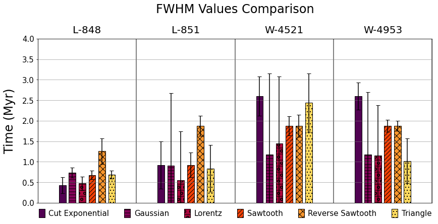
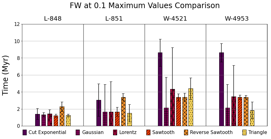
Figure 9: 3-parameter fit time width comparisons. Top: FWHM calculated for each of the 6 fits per core. Bottom: FW at 0.1 maximum height, which is closer to the true overall timescale. The errors shown are the uncertainties in the parameters: they do not reflect the goodness of the fits. A small error on a best-fit value does not indicate that this particular shape is the preferred pulse. Instead, the goodness of fit is determined by the Poisson $C_{\rm{min}}$ value (Cash, 1979).

Figure 2 shows the results for a sawtooth fit to the Ludwig core 848, and serves as an exemplar for similar plots of other cores and fits. In the top panels, we see two-dimensional slices of the $\vec{\theta}=(t_{\rm peak},\sigma_{t},\Phi_{\rm peak})$ parameter space. The red dot gives the location of the best fit, where $C(\vec{\theta})=C_{\rm min}$. The surrounding contours correspond to the 68%, 95%, and 99% confidence-level values. We see that the best-fit regions are relatively compact, meaning that the best fit is well determined. The peak flux and peak time values are the best determined, with quite small uncertainties. The width parameter shows a broader distribution and hence larger uncertainty. These trends are reflected in the bottom panel of Fig. 2, where we give the one-dimensional marginalized likelihood distributions such as

$${\cal L}(t_{\rm peak})\propto\int{\cal L}(t_{\rm peak},\sigma_{t},\Phi_{\rm peak})\ d\sigma_{t}\ d\Phi_{\rm peak}\ \ .$$ (10)

We see that unlike the well-determined peak time and flux, the sawtooth width distribution shows a rapid rise and a long tail toward long durations.

The middle panel of Fig. 2 shows the data for this core, overlaid with the curve for the best-fit parameters. We see that this optimal sawtooth function “turns on” essentially at the earliest nonzero measurement (largest time before present), denoted $t_{\rm first}$ in Table 1. The sawtooth onset is the peak time $t_{\rm peak}$, and so for the best fit, this essentially is set by the first nonzero measurement. The best-fit curve goes to zero soon after the last nonzero point (smallest time before present). This means that the width parameter $\sigma_{t}$ is in this case essentially set by the time interval between the first and last nonzero measurements shown in Table 1. We see that the height of the sawtooth at onset is a compromise among the data points so that, unsurprisingly, the measurements with the smallest errors determine the peak height $\Phi_{\rm peak}$ and also influence the slope and hence the width.

We can understand the broad width $\sigma_{t}$ distribution for this and other sawtooth fits by considering the interplay between the data and the best-fit curve in the middle panel of Fig. 2. The nonzero measurements exact a “cost” in goodness of fit $C$ for models that miss them, with the most extreme case being outright rejection ($C\rightarrow\infty$) of models that predict zero flux where counts are nonzero. Conversely, the points with zero counts impose a cost in $C$ for fits that are nonzero, but this penalty is less severe, corresponding to allowing for Poisson fluctuations. This means that sawtooth fits will be highly suppressed if they are narrower than the nonzero count data, but will have some freedom to extend beyond the width of the data, until the available zero-count points suppress fits that are much wider than the data. This is the trend we see in the width distribution.

These insights from Fig. 2 elucidate also the trends in sawtooth fits to the other sediment cores. Fig. 3 shows sawtooth fits for Ludwig core 851. Here again we see that the peak time and peak flux values are fairly well determined; though the top and bottom panels show that the peak time has a sharp lower limit, but its distribution extends for about 0.4 Myr beyond this. We can understand this feature from the middle panel: there is a lack of data between the earliest measured nonzero point and prior zero-points. This gap is about 0.3 Myr, and the lack of data here means that there is no penalty for fits that have an onset $t_{\rm peak}$ anywhere in this range. This leads to the width in $t_{\rm peak}$.

Even more striking is the width parameter in Fig. 3: we see in the bottom panel that the width distribution comes to a peak at 1.84 Myr, but the distribution is highly skewed. The $\sigma_{t}$ likelihood cuts off rapidly below the peak, but shows a long tail beyond the peak that extends out to the longest values that were allowed. Again, the data in the middle panel show the reason: after the last nonzero point (earliest time before present), there is only a single point with zero counts. Thus there is little penalty for fits with a width extending far beyond the interval between the nonzero points. Furthermore, the scatter of the nonzero points allows for a wide range of slopes, which also permits large widths. The lesson here is clear and reasonable: to get a strong constraint on the width is it essential to measure multiple points with zero ${}^{60}{\rm Fe}$ counts before and after the points with nonzero counts. For Ludwig core 848, this is the case, and the width is better constrained than that of Ludwig core 851.

This lesson is underscored when we consider Figs. 4 and 5, which show sawtooth fits to Wallner cores 4521 and 4953 respectively. For both cores, we see that effectively we can only set a lower limit to the width parameter. That is, the width likelihood in the bottom center panel begins to rise after some minimum $\sigma_{t}$, and continues to increase up to the highest allowed value. Looking at the data, we see that both cores have no points with zero counts before or after the nonzero counts. Thus, the nonzero count duration sets a lower limit to the width, corresponding to the onset of the likelihood rise, about $(1.6,2.5)$ Myr for cores (4521, 4593). However, the available data essentially set no upper limit to the width for these cores. We also see that the peak time is poorly constrained, again due to the lack of zero-count data at times earlier than the first nonzero point.

We have produced plots in the style of Figs. 2–5 for the other fitting functions. For brevity we show here only the Gaussian fit to Ludwig core 848, which appears in Fig. 6. The main trends are similar to those we saw for the sawtooth fit to this core in Fig. 2, and the peak width and peak flux are quite well determined. For the Gaussian case, we also find that the width is well determined, better than the sawtooth case. For the cores not shown, it is illuminating to compare the trends in the Gaussian fit to those found in the sawtooth fits shown in Figs. 3–5. For the Ludwig core 851, the peak time and width are broader than those in core 848, but are still well determined. On the other hand, for Wallner core 4521, the Gaussian fits also give only a lower limit to the width, and the peak time likelihood does have a clear maximum but broad tails on either side. Interestingly, the Wallner core 4953 fits are better determined, with the width and other likelihoods showing clear peaks and wings that go to zero on both sides. We believe this is due to the effect of a few nonzero points with high-precision fluxes, which anchor the Gaussian fit and prevent large excursions away from the best-fit region.

Among the other fits we tried, the reverse sawtooth case also deserves mention. Here the fit has a linear rise at early times, ending with an abrupt cutoff at late times; this was chosen to contrast with the more physically motivated sawtooth case. For these fits, we find that the width parameter likelihoods set only lower limits for all cases. This includes the Ludwig cores for which it had been possible to determine the width in the ordinary sawtooth case.

Figure 7 summarizes the best-fit curves for the six different fitting functions. Several trends emerge. Regarding the pulse widths, we see that, for the symmetric functions (Gaussian, Lorentzian, triangle), the best-fit curves all span at least 1 Myr, with Wallner cores spanning $>2\rm\ Myr$. For the asymmetric functions (sawtooth, reverse sawtooth, cut exponential), the best-fit curves are generally even wider. The initial signal arrival is sharply defined in the sawtooth and cut exponential cases, where it exceeds 3 Mya for at least one Wallner and one Ludwig core. In the other cases, the onset is gradual but also begins no later than 3 Mya.

Turning to the signal amplitude, we see that in all cases the Wallner peak fluxes are higher than those of Ludwig. These differences were discussed in §2, and may point to geophysical differences in ${}^{60}{\rm Fe}$ fallout, and could also reflect differences in ${}^{60}{\rm Fe}$ extraction techniques. We note that the ${}^{60}{\rm Fe}$/Fe ratios in the two Ludwig sediments are similar, as are the isotope ratios in the two Wallner sediments. The differences between the fluxes in the two Ludwig (and two Wallner) cores are thus largely due to the differences in sedimentation rates. For example, the sedimentation rate for L-848 is a factor $\sim 3$ lower than that of L-851. These differences propagate to our fits summarized in Fig. 7, with the Gaussian and Lorenzian profiles showing similar ratios. But the fit shape has an influence, as the triangle fits give lower ratios of peak flux, particularly for the Wallner cores, while the cut exponential and sawtooth fits give larger ratios. 

To provide a basis for comparing quantitatively the different fits for each core, we compiled all of the best-fit $C_{\rm{min}}$ values for the six fits shown in Fig. 8 and Table 2; for each data set, $C$ measures the negative of the log of the likelihood, in a close analogy to a $\chi^{2}$ for continuous data. The minimum value $C_{\rm{min}}$ thus identifies the point of maximum likelihood, playing the role of the minimum $\chi^{2}$. We note that, for a given core, $C_{\rm{min}}$ quantifies goodness of fit, in that the more negative the $C_{\rm{min}}$ value, the better the fit. As with $\chi^{2}$, variations of $C-C_{\rm min}\lesssim 1$ around the minimum are not statistically significant, while larger variations indicate a preference for the model with lower $C_{\rm{min}}$ . We also note that, while the $C_{\rm{min}}$ can be compared between fits for the same core, it is not appropriate to compare the relative $C_{\rm{min}}$ values for fits between different cores (for example, the fact that the $C_{\rm{min}}$ values for the Ludwig cores are above zero and the $C_{\rm{min}}$ values for the Wallner cores are below zero says nothing about the relative goodness of fits to the Wallner and Ludwig cores). In Table 2, the most negative value for each core has been shown in boldface. We show in italics $C_{\rm{min}}$ values that are nearly identical for the respective core have been shown in italics, indicating that the respective fit functions for the bold and italic values are all of similar quality.

We find that, for Wallner Core 4521, the triangle, Gaussian, and Lorentz fits are all equally good. As seen in Fig. 4, the data for Core 4521 are quite irregular, which could account for the multiple favorite fit shapes. Wallner Core 4953 also has a preference for the triangle and Gaussian fits. Meanwhile, the Ludwig Cores 848 and 851, which are more heavily sampled than the Wallner cores, have a clear preference for the sawtooth and Lorentz fits, respectively. The main takeaway from these results is that the ${}^{60}{\rm Fe}$ pulse does not have a preferred shape, even across the same core. Although we frequently describe the widths of the six fitting functions as the width timescales, it should be noted that these are not actually good measures for comparing different fit shapes. For example, $\sigma_{t}$ for the sawtooth fit is the full width (FW) of the fitting function and therefore is the actual timescale for that curve shape. However, $\sigma_{t}$ for the Gaussian is not given directly by the actual start and stop times of the function, since the Gaussian never reaches zero flux. Therefore, in order to compare the timescales for each function (and find a preferred time width for the supernova pulse), we have examined the traditional FW at half maximum time for each fit for each core. Since our primary interest is the maximum width of the function, we have also plotted the FW at 0.1 the maximum (which is closer to the true timescale). Table 3 and Fig. 9 show differences in the width determination between the Wallner and Ludwig samples. The values corresponding to the best-fit $C_{\rm{min}}$ values from Table 2 are also given in boldface and italics where relevant. As we have noted, these reflect differences in sampling rather than a true discrepancy; hence the robust conclusion is the lower limit this places on the signal duration.

Thus the presently available sediment data carry enough uncertainty (particularly in sampling) to prevent an unambiguous measurement of the preferred shape or timescale for all cores. As future measurements are made, these questions will become all the more important, because a demonstrated consistency among the measurements will allow us to probe the underlying astrophysics.

Our key result is that the FW at 0.1 maximum height, for all functions and cores, shows that the width of the deposition timescale is at least 1 Myr. This is significantly longer than the prediction of the traditional Sedov model.

Table 2: Goodness of Fit: $C_{\rm{min}}$ Values for 3-parameter fits.

	$C_{\rm{min}}$ Values
	Wallner et al. (2016)		Ludwig et al. (2016)
Model	Core 4521	Core 4953	Core 848	Core 851
Cut Exponential	-311.17	-158.58	63.33	30.32
Gaussian	-312.56	-174.25	62.24	26.55
Lorentz	-312.45	-173.15	65.04	24.62
Sawtooth	-311.02	-158.26	57.73	29.00
Reverse Saw	-311.72	-153.66	80.61	39.01
Triangle	-312.59	-174.34	59.85	25.56

The most negative $C_{\rm{min}}$ value for each core gives the best fit, which is shown in boldface. Fits that have nearly identical $C_{\rm{min}}$ (for the respective core) are in italics. Best-fit values should be compared between models for the same core (vertical columns), and not between cores (horizontal rows).

Table 3: Best-fit Timescale Width Values for 3-parameter fits.

	FWHM (Myr)
	Wallner et al. (2016)		Ludwig et al. (2016)
Model	Core 4521	Core 4953	Core 848	Core 851
Cut Exponential	2.60 $\pm$ 0.48	2.60 $\pm$ 0.33	0.42 $\pm$ 0.20	0.92 $\pm$ 0.58
Gaussian	1.17 $\pm$ 1.97	1.17 $\pm$ 1.52	0.73 $\pm$ 0.13	0.91 $\pm$ 1.76
Lorentz	1.45 $\pm$ 1.63	1.15 $\pm$ 1.24	0.47 $\pm$ 0.17	0.55 $\pm$ 1.20
Sawtooth	1.88 $\pm$ 0.24	1.88 $\pm$ 0.14	0.68 $\pm$ 0.10	0.92 $\pm$ 0.30
Reverse Saw	1.88 $\pm$ 0.27	1.88 $\pm$ 0.12	1.26 $\pm$ 0.31	1.88 $\pm$ 0.24
Triangle	2.44 $\pm$ 0.71	1.02 $\pm$ 0.55	0.69 $\pm$ 0.09	0.83 $\pm$ 0.57
	FW at 0.1 Maximum (Myr)
Cut Exponential	8.63 $\pm$ 1.59	8.63 $\pm$ 1.09	1.41 $\pm$ 0.65	3.04 $\pm$ 1.91
Gaussian	2.14 $\pm$ 3.59	2.14 $\pm$ 2.77	1.34 $\pm$ 0.23	1.66 $\pm$ 3.21
Lorentz	4.34 $\pm$ 4.90	3.44 $\pm$ 3.71	1.42 $\pm$ 0.50	1.65 $\pm$ 3.59
Sawtooth	3.38 $\pm$ 0.43	3.38 $\pm$ 0.26	1.22 $\pm$ 0.19	1.66 $\pm$ 0.54
Reverse Saw	3.38 $\pm$ 0.49	3.38 $\pm$ 0.22	2.27 $\pm$ 0.56	3.38 $\pm$ 0.44
Triangle	4.40 $\pm$ 1.28	1.84 $\pm$ 0.99	1.23 $\pm$ 0.17	1.50 $\pm$ 1.03

Values in boldface match the best-fit $C_{\rm{min}}$ in Table 2; similarly, values in italics are nearly identical best fits for that core. The errors are 1$\sigma$.

3.3 Terrestrial and Geophysical Effects—Is the Signal Width of an Astronomical Origin?

We now discuss how terrestrial and geophysical effects might smear the timescale of the ${}^{60}{\rm Fe}$ pulse.

The atmosphere. When the dust, which is traveling at up to 100 km s^-1, hits the Earth’s atmosphere, it is vaporized. The iron atoms then combine in the upper atmosphere with molecules such as ozone and hydroxyl radicals, and are eventually deposited on land and in the ocean. Fry et al. (2016) provides excellent approximations for the residence times of the iron in the atmosphere and demonstrates that the iron settles out of the atmosphere in less than 10 yr.

Deposition on land. There is no currently known way to detect the ${}^{60}{\rm Fe}$ signal on land, unless it is deposited on an ice sheet, e.g., in Antarctica, where ongoing deposition has recently been measured (Koll et al., 2019).

Deposition in the ocean. The residence, i.e., removal, time of iron in the ocean is relatively short, on the order of $\sim$ 500 years at most (Bruland et al., 1994; Boyle, 1997; Resing et al., 2015). When the dust settles on the ocean floor, it may be taken up by FeMn crusts or deposited as sediment.

FeMn Crusts. Once iron is absorbed by a FeMn crust, it remains “locked-in” and unchanged until analysis, and the time signal is accurately preserved. However, due to the slow growth rate, it is very difficult to time resolve FeMn crusts on the order of kyr, and only the recent work of Wallner et al. (2021) has done so. There is also the possibility of crust porosity, which would enable the iron to attach below the surface, thus smearing the signal.

Sediments. It is possible to resolve the time structure of deposits in sediments on the order of kiloyears, but there are a number of effects that can smear the time signature. The two most important are bioturbation (the churning of the upper few layers of sediment by macroscopic organisms) and chemical reducing environments (created by bacteria and leading to the movement of iron within the sediment column). However, all the sediment samples we consider are from the deep sea where bioturbation effects are negligible, and were carefully selected to ensure that a reducing environment did not occur (Fitoussi et al., 2008; Ludwig et al., 2016).

In summary, there are a number of geochemical, geophysical, oceanic, and biological effects that can in principle distort the ${}^{60}{\rm Fe}$ timescale. However, the combination of these effects is less than $\Delta t\sim 10^{3}$ yr, which is far shorter than the $\Delta t\sim 10^{6}$ yr timescale found in the data. We conclude, therefore, that the measured timescale must be astrophysical in origin. Accordingly, we need a model for the origin and transport to Earth of the dust that can accommodate the signal width and might also be able to predict the line shape, which could be constrained by future data with higher precision.

3.4 Multiple supernovae?

There is significant interest in analyzing the possibility of multiple supernovae to account for the signal $\sim 3$ Myr ago, e.g., Breitschwerdt et al. (2016) and Schulreich et al. (2018) propose that some 16 to 19 supernovae have exploded in the Local Bubble, and have contributed to the extended ${}^{60}{\rm Fe}$ signal. Unfortunately, the data are too noisy to cleanly distinguish multiple superposed supernovae peaks. We have seen that the sediment measurements cannot unambiguously distinguish the relatively simple pulse shapes we have tried, which have shapes as different as possible for a singly peaked structure. Thus, the data in hand cannot exclude a more complex pulse shape that would superpose multiple supernova pulses.

Despite these limitations, the ${}^{60}{\rm Fe}$ data carries substantial information bearing on the question of multiple supernovae creating the observed 3 Myr pulse. In particular (a) singly peaked pulse shapes provide adequate descriptions of the measurements, and (b) none of the data show clear groupings of points within the time range of detected points. The available data are thus consistent with a single peak, and do not require multiple events.

Furthermore, an accounting for the ${}^{60}{\rm Fe}$ data must explain not only the long signal width seen in the samples but also the discovery of distinct pulses at 3 and 7 Myr, with no apparent signal in between. If there are multiple events in the 3 Myr peak, then there would likely need to be a similar set of events for the 7 Myr peak, but then the gap between the two would need explanation. These considerations will inform models for multiple supernovae, but do not rule them out.

We do not consider it a productive exercise to fit for multiple supernovae given the limitations of the available data, so we restrict our analysis to a single supernova. We discuss models for the pulse width below in §4.

Additional time-resolved measurements of the 3 Myr ago signal (such as could be provided by more dense sampling) could help enormously, but would require significant extra efforts beyond those already made to gather the current data set. Another possibility would be to measure the fluxes of additional isotopes across the ${}^{60}{\rm Fe}$ signal region. If there were significant variations in the isotope ratios, these could constitute evidence for multiple supernovae with different combinations of nucleosynthesis mechanisms.

3.5 Four-parameter Fit

In order to examine the ambiguity of the preferred fit shape for the data, we include a 4-parameter “sharktooth” fit in our analysis. The purpose of this fit is to analyze whether the data is better described by an asymmetric shape, and at what level of preference. We chose to work with a 2-width triangle shape, of which the sawtooth, reverse sawtooth, and symmetric triangle are the three-parameter extremes. The function is defined below in Appendix A. The shape was given the full range from almost full sawtooth to almost full reverse sawtooth, with only a minor initial minimum of 0.05 Myr to prevent either width from being zero. As with the 3-parameter fits, we also enforced a maximum total width of 3.5 Myr, which is clearly seen to be relevant for Wallner Core 4521 in Fig. 11. This width cap is to prevent the fit from stretching all the way to $t=0$ Myr for the noisier data, and was picked as the minimum width needed before the triangle shapes stopped changing dramatically.

Results for the Ludwig 851 core appear in Fig. 10. We see in the bottom panels that the two widths have well-defined peak likelihoods, but broad distributions. In the upper left panel, we see that the two widths have some anticorrelation, as one might expect if they have to at least sum to the spread in the nonzero data points.

Examining the best-fit shapes for the four cores in Fig. 11, we can see that most of the data are best fit with a sharktooth shape that is intermediate between being fully symmetric or asymmetric. Only Ludwig Core 848 prefers a perfect sharp sawtooth shape, with the fit function capped by the minimum width initial parameter. The two Wallner cores prefer a slightly sawtooth shape, while Ludwig Core 851 actually has a slight preference toward a reverse sawtooth.

It should be noted once again that the sharktooth fits are not statistically comparable to the 3-parameter fits in §3.2. However, in view of the lack of strong preference for a specific 3-parameter fit, it is an interesting possibility to explore further. Given the variations in the current data, we cannot meaningfully pick a preferred shape for the ${}^{60}{\rm Fe}$ pulse, so the pulse shape does not provide significant information on the underlying astrophysics. However, the different pulse widths extracted using the different preferred fit shapes can be used to make some inferences on the astrophysical processes inside the supernova remnant.

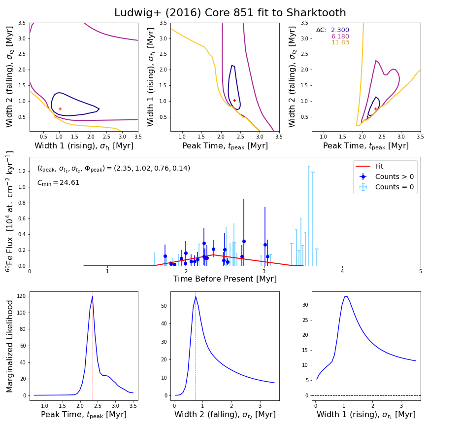
Figure 10: 4-parameter sharktooth fits to the terrestrial ⁶⁰Fe flux of Ludwig et al. (2016). The figure is formatted similarly to the 3-parameter fits, with the two width parameters and the peak time analyzed. Width 1 ($\sigma_{t_{1}}$) is the rising width for the sharktooth, i.e., the time elapsed between the start of the infall and the peak, and Width 2 ($\sigma_{t_{2}}$) is the time elapsed from the peak until the end of the infall.

Figure 11: 4-parameter sharktooth fits to the terrestrial ⁶⁰Fe flux.

3.6 Global Fits

Figure 12: Global fit to all well-sampled sediments, using a sawtooth profile for the flux. The width is fixed, but the peak flux and peak time are both allowed to vary, allowing for nonuniform global dust fallout and systematic errors in absolute timing, respectively.

Having examined the cores individually, we now turn to global fits that use all the cores to analyze jointly the ${}^{60}{\rm Fe}$ deposition history. To do this, we first note that the ${}^{60}{\rm Fe}$ flux time profile (i.e., its shape) should be common to all of the sediments regardless of their location on the Earth. We therefore fit all of the samples using a single pulse shape and thus the same width parameter $\sigma_{t}$.

Table 4: Global Fit Parameters

		Fit Type
Parameter		Gaussian	Sawtooth	Triangle
Width parameter $\sigma_{t}$	[Myr]	$0.47\pm 0.05$	$3.18\pm 0.26$	$0.99\pm 0.10$
Full width at 0.1 max $\Delta t$	[Myr]	$2.00\pm 0.21$	$2.86\pm 0.23$	$1.8\pm 0.2$
$\Delta t$ 95% CL lower limit	[Myr]	$1.7$	$2.7$	$1.6$
Peak time $t_{\rm peak}$ [Myr]	L-848	$2.16\pm 0.10$	$2.7\pm 0.05$	$2.1\pm 0.09$
	L-851	$2.44\pm 0.11$	$3.2\pm 0.2$	$2.4\pm 0.9$
	W-4521	$2.12\pm 0.11$	$3.3\pm 0.5$	$2.2\pm 0.9$
	W-4953	$2.44\pm 0.05$	$3.5\pm 0.2$	$2.5\pm 0.4$
Peak flux $\Phi_{\rm peak}$ [atoms cm-2 kyr-1]	L-848	$0.037\pm 0.006$	$0.039\pm 0.021$	$0.042\pm 0.007$
	L-851	$0.116\pm 0.019$	$0.13\pm 0.04$	$0.12\pm 0.02$
	W-4521	$3.89\pm 0.41$	$6.0\pm 1.9$	$4.5\pm 0.5$
	W-4953	$3.19\pm 0.42$	$2.7\pm 0.5$	$3.6\pm 0.5$
Fluence ${\cal F}_{60}$ [$\rm 10^{7}\ atomscm^{-2}$]	L-848	$0.043\pm 0.07$	$0.060\pm 0.023$	$0.041\pm 0.007$
	L-851	$0.14\pm 0.03$	$0.19\pm 0.05$	$0.12\pm 0.02$
	W-4521	$4.4\pm 0.6$	$9.5\pm 3.2$	$4.4\pm 0.6$
	W-4953	$3.7\pm 0.4$	$4.4\pm 0.8$	$3.6\pm 0.3$
Goodness of fit	$C_{\rm{min}}$	-195.5	-185.6	-196.8

Fits with a single width parameter but varying peak times and peak flux values for different cores. L denotes Ludwig et al. (2016), W denotes Wallner et al. (2016). We list below the best-fit values and 1$\sigma$ uncertainties. The peak flux is given in units of $10^{4}$ atoms cm^-2 kyr^-1, and the fluence in units of $10^{7}$ atoms cm^-2. For the goodness of fit $C_{\rm{min}}$ , bold indicates the highest likelihood, and italics the close second.

We account for potential systematic differences between the samples by allowing the other fit parameters to vary independently for each core. To include possible systematic offsets in the absolute dating of the different samples, we fit different peak times for each core; this would correspond to shifts in the inferred time history between the samples. Small differences in the peak times of individual fits would suggest that differences in the dating are small, but large differences would point to the presences of unaccounted systematics, or the use of a bad fitting function. We also allow for differences in the peak heights, which could arise due to different infall and uptake at different locations. To perform these fits, we use a Markov Chain Monte Carlo approach, which enables us to search efficiently the 9-dimensional parameter space using the emcee package (Foreman-Mackey et al., 2013).

Fig. 12 shows our results for the case of a sawtooth time profile; the best-fit parameters and other statistics are given in Table 4. Turning first to the width, we see that the likelihood is zero until about 2 Myr, then rises until the highest allowed value. Thus, as we have seen with the individual fits in Figs. 2–5, the global sawtooth form only sets a lower limit to the signal width. We find that the 95% confidence lower limit to the FW at 0.1 maximum is 2.7 Myr. This limit is significantly larger than the time span of nonzero data points shown in Table 1, showing that the requirement of a sawtooth form leads to wider deposition time.

The shapes of the peak times are similar to those in the individual core fits in Figs. 2–5, and show the same asymmetries. We find that the most probable peak times differ significantly among the samples. This reflects the fact that, for a sawtooth, the peak is also the point with the earliest nonzero ${}^{60}{\rm Fe}$ counts, itself an artifact of the sampling. These differences between the peak times (upper right panel of Fig. 12) are also similar to those in the individual fits.

The peak ${}^{60}{\rm Fe}$ flux values (lower left panel) and the ${}^{60}{\rm Fe}$ fluences (lower right panel) measured in the two Wallner samples are similar, and also those of the two Ludwig samples. However, we do see significant differences in the peak ${}^{60}{\rm Fe}$ flux values (lower left panel) and the ${}^{60}{\rm Fe}$ fluences (lower right panel) between the Wallner and Ludwig measurements. As noted above, this may be due to differences in the analysis techniques, and also perhaps due to differences in the deposition rates caused by varying infall or uptake factors. We note that the global sawtooth fits for the Wallner cores give values that are slightly higher than in the individual fits, but well within errors.

We have also performed global fits for the Gaussian and triangle fit functions. The results are summarized in Table 4, and the Gaussian fit is shown as Fig. 14. For the Gaussian case, we see that the FW at 0.1 maximum of $2.00\pm 0.21\ \rm Myr$ (upper left panel) is a compromise between the values of the Gaussian widths found in individual sample fits as seen in Table 3. On the other hand, the triangle case gave a well-determined width, similar to the global Gaussian fit and the individual triangle fits. We find that, for the Gaussian fit, the 95% confidence-level lower limit to the FW at 0.1 maximum is 1.7 Myr, while for the triangle fit the same limit is 1.6 Myr. The upshot is that, for these other functional forms, the global fits once again give a long timescale for the ${}^{60}{\rm Fe}$ deposition. Thus, using all of the data, we find that the pulse timescale is at least

$$\Delta t>1.6\ \rm Myr\,,$$ (11)

which is also close to the interval between the earliest and latest nonzero ${}^{60}{\rm Fe}$ counts across all crusts shown in Table 1. Any model for ${}^{60}{\rm Fe}$ delivery must account for this timescale.

For the Gaussian and triangle global fits, we also find that the peak time and peak flux values for each sediment are similar to those for the corresponding single-sediment fits seen in Figs. 2 to 6. The differences among the peak times are relatively small, with significant overlaps between the different fits. This suggests that the absolute dating of the various samples does not suffer from significant unknown systematic uncertainties. This also supports our conclusion that the differences in peak times in the sawtooth case (Fig. 12) are due to the abrupt onset of that fitting form, and the sampling.

Turning to the fluence, Table 4 shows that the Gaussian and triangle results are very similar, indicating that the integral nature of the fluence is not very sensitive to the differences between these fitting functions. On the other hand, the sawtooth case gives substantially higher fluences for all sediments. Since the sawtooth fluence is given by $\Phi_{\rm peak}\,\sigma_{t}/2$, and the peak flux values are consistent across different fitting function, it is clear that the timescale $\sigma_{t}$ is the source of the discrepancy. Indeed, we have seen that the sawtooth timescale is poorly determined by individual fits in Figs. 2–5. For this reason, we see that determinations of the fluence are model-dependent given the current data.

In sum, we see that when all of the sediment data are combined; the global fits find that the ${}^{60}{\rm Fe}$ fallout time is long, $\approx 2\ \rm Myr$. We recall that, as discussed in §3.3, this duration is not a geophysical artifact, but reflects the underlying astrophysical fallout time. We now turn to the interpretation of this result.

4 Implications: Supernova Dust Formation and Propagation

The timescale for ${}^{60}{\rm Fe}$ deposition encodes information about the delivery of supernova ejecta from the explosion to its final arrival at Earth. Moreover, we recall that for supernova material to reach Earth it must take the form of dust grains (Athanassiadou & Fields, 2011). This means the ${}^{60}{\rm Fe}$ fallout timescale is a probe of the propagation of supernova dust over space and time.

We consider in this section two scenarios for supernova dust formation and evolution. (1) The first scenario adopts the conventional assumption, often implicit, that supernova dust is entrained in the gas and thus is comoving with the blast (e.g., Fry et al., 2015; Breitschwerdt et al., 2016, make this assumption). (2) The other scenario is the model of Fry et al. (2020) in which the dust decouples from the gas, and the trajectories of the charged grains are determined by the magnetic structure of the remnant. We develop predictions for the time history of the dust flux in these two models, which can then be compared with the measured ${}^{60}{\rm Fe}$ time profiles.

4.1 Dust Entrainment Model

In this picture, the dust grains move with the gas, so that the grain velocity is the same in magnitude and direction as the plasma bulk velocity $v_{\rm gr}=v_{\rm gas}$, i.e., the motion is radial, overlaid with perturbations due to turbulence. In addition, we assume the mass density $\rho_{\rm dust}$ of dust grains is always proportional to the gas density $\rho_{\rm gas}\approx m_{p}n_{\rm gas}$. This model thus posits a direct proportionality between the mass fluxes of the grain particles and the gas: $J_{\rm gr}=\rho_{\rm dust}v_{\rm gr}\propto\rho_{\rm gas}v_{\rm gas}$. Thus, the time history of the grain flux is determined by that of the gas flux.

This model is the one adopted by Fry et al. (2015), whose key results we summarize here. The model focuses on the Sedov phase of the remnant, in which the blast radius evolves as follows as a function of time $t$: $r_{\rm blast}=\beta(Et^{2}/\rho)^{1/5}$, where $E$ is the kinetic energy of the ejecta into a uniform-density medium with $\rho=\bar{m}n$, and $\beta=1.1517$ for monatomic gas, with adiabatic index $\gamma=5/3$. Inverting this relation, we derive the following estimate of the blast arrival time at radius $r$:

$$t_{\rm blast}=\beta^{5/2}\sqrt{\frac{\rho r^{5}}{E}}=0.036\ {\rm Myr}\ \left(\frac{\bar{m}}{m_{p}}\right)^{1/2}\ \left(\frac{n}{0.01\ \rm cm^{-3}}\right)^{1/2}\ \left(\frac{10^{51}\ \rm erg}{E}\right)^{1/2}\ \left(\frac{r}{50\ \rm pc}\right)^{5/2}\,,$$ (12)

where we scale using benchmark estimates of the Local Bubble density and total blast energy (see, e.g., Fry et al., 2020). The corresponding speed of expansion is

$$v_{\rm blast}=\frac{2}{5}\frac{r}{t}=\frac{2}{5}\sqrt{\beta\frac{E}{\rho r^{3}}}=550\ {\rm km/s}\ \left(\frac{m_{p}}{\bar{m}}\right)^{1/2}\ \left(\frac{0.01\ \rm cm^{-3}}{n}\right)^{1/2}\ \left(\frac{E}{10^{51}\ \rm erg}\right)^{1/2}\ \left(\frac{50\ \rm pc}{r}\right)^{3/2}\,.$$ (13)

Just behind the shock, the gas density is always the same constant multiple of the ISM density, namely $\rho_{\rm gas}=4\rho_{\rm ism}$ for $\gamma=5/3$. However, because the mass of the supernova ejecta is fixed initially, the ejecta density must drop as the blast volume grows. To fix numbers, we assume that the ejecta are entrained with the gas, and approximate the blast as a thin uniform-density shell of fractional width $x=\Delta r_{\rm shell}/r_{\rm blast}\ll 1$, in which case mass conservation implies $x\approx 1/12$.

The duration of the flux is the timescale for the blast shell to pass by. At a fixed distance $r$, and using self-similarity, the shell crossing time is

$$\Delta t_{\rm shell} \approx \frac{xr}{v(r)}=\frac{5x}{2}t\approx\frac{5}{24}t$$ (14)

$$= 0.03\ {\rm Myr}\ \left(\frac{m_{p}\times 0.01\ \rm cm^{-3}}{\rho}\right)^{1/2}\ \left(\frac{E}{10^{51}\ \rm erg}\right)^{1/2}\ \left(\frac{100\ \rm pc}{r}\right)^{5/2}\,.$$ (15)

This is nearly two orders of magnitude smaller than the observed ${}^{60}{\rm Fe}$ pulse width.

The ISM density would have to be $\gtrsim 100\ \rm cm^{-3}$ in order to overcome this discrepancy. Such a density is characteristic of a giant molecular cloud complex, which could have been a plausible density if our ${}^{60}{\rm Fe}$-depositing supernova were the first to explode in a nearby star-forming region. However, modeling of the Local Bubble indicates that it has hosted multiple supernovae over timescales of 3 Myr or longer (Smith & Cox, 2001; Breitschwerdt et al., 2016), and there is now clear evidence for ${}^{60}{\rm Fe}$ deposition by an explosion $\sim 7$ Mya (Wallner et al., 2021). After the first explosion, the local interstellar region would have a much smaller density, so we are driven to consider other explanations for the long ${}^{60}{\rm Fe}$ timescale.

It is also worth highlighting that terrestrial (anthropogenic) explosions do not exhibit efficient mixing of ejecta with the larger blast wave. Although both move outward rapidly, the ejecta (i.e., the material responsible for the explosion) remains confined relatively near the center of the explosion while the forward shock travels much greater distances and without carrying ejecta material with it. For example, in the case of the Chelyabinsk bolide, the larger meteorite fragments were found in a 32-km long, 10 km wide region along the original trajectory of the meteor (Popova et al., 2013). Meanwhile, the smaller aerosols and dust particles formed a cloud that rose vertically 11 km over 80 s then stabilized at that altitude for the next 120 s (Gorkavyi et al., 2013). In contrast, the shock wave produced by the bolide propagated radially outward traveling 23 km in 76 s and 52 km in 173 s (Popova et al., 2013) showing a definitive decoupling between the shock wave and ejected material. Such observations of decoupling further constrain the entrainment model’s validity.

Several possible explanations of the long ${}^{60}{\rm Fe}$ deposition timescale have been discussed elsewhere. (1) The prolongation of the signal over time could reflect multiple supernovae, each with a narrow pulse width (Breitschwerdt et al., 2016). As we have noted, the data does not demand this, but also cannot exclude multiple supernovae in the 3 Myr peak. However, because we observe a broad ${}^{60}{\rm Fe}$ pulse $\sim 3$ Mya, preceded by a gap and and another pulse $\sim 7$ Mya that also seems broader than suggested by the entrainment model (12), this scenario would require two bursts of supernovae in rapid sequence, with a well-defined lull in between. (2) The ${}^{60}{\rm Fe}$ flux could reflect the motion of the Sun through the supernova material (Chaikin et al., 2022), with a complex time history needed to accommodate the two broad pulses. (3) Another possibility is that some ${}^{60}{\rm Fe}$-bearing dust was trapped by the Local Interstellar Cloud, an $\sim 5$ pc feature that envelops the solar system (Koll et al., 2019; Linsky et al., 2019). One can quantify this by considering the stopping power of the cloud. For dust grains the size $a_{\rm gr}\gtrsim 0.3\,\rm\mu m$ needed to overcome solar radiation pressure, the stopping distance due to drag is $60\ \rm pc$ for $n_{\rm LIC}=0.2\ {\rm cm}^{-3}$. Thus we do not expect drag to efficiently stop the grains unless they are much smaller. (4) Opher & Loeb (2022) model the effects of a neutral cloud (seeded with ${}^{60}{\rm Fe}$) passing through the solar system, and show that, if the cloud density is very high, it can compress the heliosphere within 1 au. If the cloud is also large enough, the passage can last for the required time.

We consider these scenarios to be worthy of further investigation, but also not without their challenges. Here we propose another solution motivated by our recent work (Fry et al., 2020), assess its merits and drawbacks, and offer observational tests.

4.2 Charged Dust Model

We propose that the ${}^{60}{\rm Fe}$ arrives at the Earth (and Moon) as part of charged dust grains that were created in the supernova, whose propagation was largely determined by the magnetic structure of the remnant impact into the surrounding medium. Fry et al. (2020) performed detailed calculations of the propagation of charged dust in a supernova remnant, motivated by the ${}^{60}{\rm Fe}$ data. Here we summarize the rich physics influencing dust grain evolution and propagation.

Dust formation in supernova remnants is a subject of intense ongoing research, but it is clear that a substantial amount of dust is formed very soon after the explosion, e.g., SN 1987A shows infrared emission consistent with all of the supernova-produced iron being locked into grains within tens of years after the explosion (Matsuura et al., 2011, 2017, 2019), while recently Niculescu-Duvaz et al. (2022) examine a large sample of supernovae finding that, after $\sim 30$ yr, on average $0.24^{+0.09}_{-0.05}\,M_{\odot}$ of material is condensed into dust. We therefore follow Fry et al. (2020) in assuming that dust is present, likely with a range of grain sizes, and initially entrained with the gas from which it formed. Thus a range of dust compositions, sizes, and velocities is present.

After the dust is created, it suffers collisions with gas particles that lead to drag, sputtering, and charging. However, these effects are minimal because the dust is comoving with the gas. But as the supernova remnant evolves, a reverse shock propagates inward. This shocks and slows the gas, thereby decoupling the dust from the gas. Grains suffer some damage at the shock, but those large enough to survive crossing the reverse shocks will then be subjected to increased drag, sputtering, and charging.

Given the negligible magnetic field in the inner portion of the supernova remnant, the dust still travels radially. However, when the dust grains subsequently encounter the magnetized ISM, it acts as a mirror and reflects the dust. The dust grains then pass back through the remnant until they encounter the ISM material once more, and are again reflected by its magnetic field (at each ISM encounter, there is also some probability that the grains become trapped). The resulting dynamics is that the dust is confined to the ejecta region, with repeated bouncing motion, “pinball” style, in the ejecta interior. As they propagate, the dust particles are slowed by drag and are sputtered, becoming smaller and losing mass.

An order of magnitude calculation illustrates the key features of dust evolution found in the Fry et al. (2020) simulations. We model a dust grain as a sphere of radius $a$, density $\rho_{\rm dust}$, and mean atomic mass $m_{\rm gr}$. As the dust particle moves through the gas, it suffers collisions at a rate

$$\Gamma_{\rm coll}=n_{\rm gas}\sigma v_{\rm rel}\approx\pi a^{2}n_{\rm gas}v_{\rm dust}\,,$$ (16)

where in the second expression we approximate the collision cross section with the geometric cross section, and assume that the dust is moving much faster than the gas, so that the relative speed $v_{\rm rel}\approx v_{\rm dust}\gg v_{\rm gas}\sim\sqrt{kT/m_{p}}$; moreover, we assume that the gas is dominated by hydrogen.

Drag has collisional and Coulomb components. In the assumed limit of fast dust particles with $m_{\rm p}v_{\rm gr}^{2}\gg kT$ the collisional term is

$$F_{\rm coll}\simeq\Gamma_{\rm coll}m_{p}v_{\rm rel}\simeq\Gamma_{\rm coll}m_{p}v_{\rm gr}\,,$$ (17)

where $\vec{v}_{\rm rel}=\vec{v}_{\rm gr}-\vec{v}_{\rm gas}$ is the grain speed relative to the local gas speed. This gives a collisional stopping time of order

$$\tau_{\rm coll} = \left|\frac{M_{\rm gr}v_{\rm gr}}{F_{\rm coll}}\right|\simeq\frac{4\rho_{\rm gr}a}{3m_{\rm p}n_{\rm gas}v_{\rm gr}}$$ (18)

$$= 3.9\ {\rm Myr}\ \left(\frac{a}{0.3\ \mu\rm m}\right)\ \left(\frac{10^{-2}\ \rm cm^{-3}}{n_{\rm gas}}\right)\ \left(\frac{300\ \rm km/s}{v_{\rm gr}}\right)\,,$$ (19)

where $M_{\rm gr}$ is the grain mass. The Coulomb drag force for high speeds larger than the plasma thermal speeds $v^{2}\gg kT/m_{p}$ is independent of grain size: $F_{\rm Coul}\approx 4\pi z_{\rm gr}^{2}\,e^{2}\,n_{\rm gas}\,\ln[\Lambda]/m_{p}v^{2}$, in contrast to the collisional drag; here $\ln[\Lambda]\sim 20$ is the so-called Coulomb logarithm. The Coulomb stopping time therefore exhibits a different and stronger dependence on grain size:

$$\tau_{\rm Coul} = \left|\frac{M_{\rm gr}v_{\rm gr}}{F_{\rm Coul}}\right|\simeq\frac{\rho_{\rm gr}a^{3}v_{\rm gr}^{3}}{3z_{\rm gr}^{2}e^{2}n_{\rm gas}}$$ (20)

$$= 2.5\ {\rm Myr}\ \left(\frac{a}{0.3\ \mu\rm m}\right)^{3}\ \left(\frac{10^{-2}\ \rm cm^{-3}}{n_{\rm gas}}\right)\ \left(\frac{300\ \rm km/s}{v_{\rm gr}}\right)\ \left(\frac{175\ \rm V}{U_{\rm gr}}\right)\,.$$ (21)

If the grain is indeed moving much faster than the gas, then sputtering decreases the grain radius at a rate

$$\frac{da}{dt}\simeq-\frac{m_{\rm gr}Y}{4\pi\rho_{\rm gr}a^{2}}\Gamma_{\rm coll}=-\frac{m_{\rm gr}n_{\rm gas}}{4\rho_{\rm gr}}Yv_{\rm dust}\,,$$ (22)

where $Y$ is the energy- or velocity-averaged yield of atoms liberated per collision, and $m_{\rm gr}$ is the mean mass of a grain atom. The resulting timescale for grain erosion due to sputtering is

$$\tau_{\rm sput}=\left|\frac{a}{\dot{a}}\right|\simeq\frac{3}{Y}\frac{m_{\rm p}}{m_{\rm gr}}\ \tau_{\rm drag}=2\left(\frac{50}{m_{\rm gr}/m_{\rm p}}\right)\frac{0.03}{Y}\ \tau_{\rm drag}\,.$$ (23)

We see that, in the high-velocity regime, the sputtering and drag timescales are related by a factor that depends only on the grain atomic mass and yields. Estimating these values for iron-bearing grains shows the timescales to be comparable, with drag somewhat faster. We thus expect significant drag and sputtering both to occur, and that the grain lifetime is similar to the drag timescale.

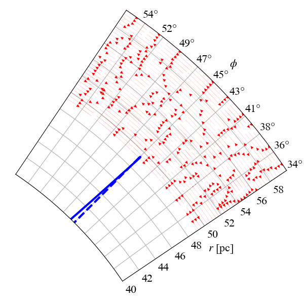
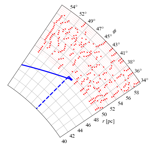
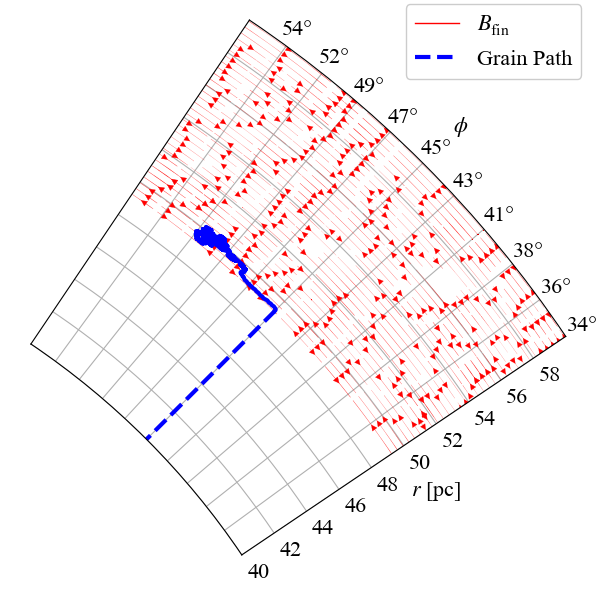
Figure 13: Three sample azimuthal trajectories from our 0.1 $\mu$m metallic Fe dust grain simulations. The left panel shows a grain being bounced (reflected off) the magnetic field in the ISM, and the center panel shows a grain becoming temporarily trapped by the ISM magnetic field before eventually escaping. Finally, the right panel shows a grain becoming trapped by the ISM magnetic field for the duration of the simulation. The grain path is shown as a dashed blue line until reflection, and a solid blue line afterwards. The red lines are the magnetic field lines at the moment of reflection ($t\approx 130$ kyr, $r\approx 50$ pc after the supernova).

Figure 13 shows sample simulations of the trajectories of 0.1 $\mu$m dust grains (blue) encountering the magnetic field in the ISM (red). The left panel shows an example where the dust grain bounces (is reflected) straight back from the ISM, and the central panel shows an example where the dust grain is trapped temporarily by the ISM magnetic field, but eventually escapes. These exemplify the “pinball” feature discussed in Fry et al. (2020), whereby the directions of the dust grains’ trajectories can be changed, losing memory of the location of their progenitor. Finally, the third panel shows an example where the dust grain is trapped for the duration of the simulation. All three panels illustrate how the timescale for the deposition of live radioisotopes can be extended due to interactions with the ISM.

Determining quantitatively the conditions when a grain will be reflected versus trapped (and for how long) is a subject requiring further examination. A grain’s charge depends on its composition, speed, and the surrounding environment; the dynamics of the magnetic field is determined by the supernova remnant’s plasma dynamics. While the grain’s possible motions are understood (i.e., curvature drift, gradient drift, reflections, etc.), when those occur is not fully characterized. The time the grain first encounters the magnetic field, the pitch angle of the grain’s velocity with the local magnetic field, the dynamical timescale of the magnetic field, and the size of any turbulent eddies and density perturbations can influence the confinement of the dust grains. Fry et al. (2020) provided an initial statistical result for metallic iron grains, but a more detailed examination is beyond the scope of this work.

To summarize, our model builds upon the results of Fry et al. (2020) to predict the following supernova dust grain history and dynamics as the supernova remnant evolves.

• Free expansion phase: coupled. Dust grains are nucleated in dense ejecta knots, comoving with gas (Fry et al., 2020).

• Start of Sedov phase: decoupling. As the ejecta (composed of ejected gas and dust grains) experiences the reverse shock and decelerates, the surviving dust grains are dynamically decoupled from the gas. Their subsequent propagation is dominated by the Lorentz force and drag. In weakly or nonmagnetized supernova material, their motion is radial until they encounter the magnetized ISM (Fry et al., 2020).

• Sedov and snowplow phases: reflection and trapping. In encounters with the magnetized ISM, grains may be either reflected or trapped. The reflected grains traverse the inner supernova remnant until their next encounter with the ISM. Grain size plays a crucial role here: the smallest grains ($a\sim 0.005\ \mu\rm m$) are trapped at the first encounter, sputtered, and lost, whereas the largest grains ($a\sim 1\ \mu\rm m$) travel past the supernova-ISM boundary and then are trapped. Intermediate-sized grains ($a\sim 0.05-0.1\ \mu\rm m$) have non-negligible probabilities both to be trapped and to escape. Thus over time the grain number density in the supernova material will drop, in favor of a buildup of trapped grains at the supernova-ISM boundaries. The trapped dust motion depends on the grain size and potential (i.e., the charge-to-mass ratio).

• Fadeaway phase: shell buildup and release to ISM. Trapped grain motion in turbulent field lines will be approximately diffusive, leading to a buildup in a shell at the supernova-ISM boundary. Spatial and time changes in the magnetic fields can lead to grain deceleration and acceleration, in addition to the action of drag. The grains are stopped over the drag timescale. The larger grains survive and remain as the forward shock slows to a sound wave, and the supernova remnant fades.

In this picture, the spatial distribution of dust grain changes over time. While the dust grains are predominantly reflected, the grains should roughly uniformly populate the inner supernova remnant. As they become trapped in the surrounding magnetized ISM, the grains should move diffusively in a shell of increasing thickness around the inner remnant. Thus, when the grain-bearing material arrives at the solar system, we expect the particle density to be a mix of a uniform and shell profile, with the shell profile more favored at late times and large distances. Detailed modeling of this distribution, and the resulting ${}^{60}{\rm Fe}$ time profile at Earth, is beyond the scope of this paper, but is a problem we intend to revisit in future work.

5 Consequences and Tests

The sequence of events in the pinball model for supernova grain evolution has significant implications for different dust species and radioisotope signatures, as we now discuss.

Supernova distance. Rough estimates have suggested that the origin of the spike in ${}^{60}{\rm Fe}$ $\sim 3$ Mya might have been a supernova that exploded within about 100 pc of Earth. Several stellar clusters are known to have passed within 200 pc of Earth within the past 35 Myr. Two of these have attracted particular attention: the Tuc-Hor group (Mamajek, 2015; Hyde & Pecaut, 2018), which was within $\sim 60$ pc of Earth at the time of the event that produced the 3 Mya signal, and the Sco-Cen OB association (Benítez et al., 2002), which was $\sim 130$ pc away at that time — the possibility of a runaway star has also been considered. No conclusive evidence in favor of any hypothesis has been found.

Our analysis of the propagation of magnetic dust indicates that it could not progress far into the ISM. See, in particular, Fig. 4 of Fry et al. (2020), where simulations of metallic Fe grains of varying initial sizes indicate that they would reach a maximum distance of about 50 pc. This limited range favors a Tuc-Hor origin over the Sco-Cen hypothesis, while being consistent with the runaway star hypothesis.

Gamma-ray line spectroscopy of nuclear lines. There have been multiple observations of gamma rays from decays of ${}^{60}{\rm Fe}$ and ${}^{26}{\rm Al}$ in the ISM. In our model, the dust bearing ${}^{60}{\rm Fe}$ and ${}^{26}{\rm Al}$ dust moves at high speeds within the supernova remnant for much of the radioactive lifetime of the species. Therefore we would expect the ${}^{60}{\rm Fe}$ and ${}^{26}{\rm Al}$ nuclear lines to exhibit Doppler broadening. Indeed, International Gamma-Ray Astrophysics Laboratory (INTEGRAL) data indicate that the line width of ${}^{26}{\rm Al}$ decay is broadened (Kretschmer et al., 2013). If the dust drag time reflects the ${}^{60}{\rm Fe}$ width, then our work shows that the stopping timescale $\gtrsim 1\ \rm Myr$. This is longer than the 0.717 Myr half-life of ${}^{26}{\rm Al}$, which means that most of the ${}^{26}{\rm Al}$ in supernova dust will decay while moving at high speed, consistent with the INTEGRAL result.

Supernova remnants. If supernova dust grains are only created at early times, then the dust mass in the ejecta itself should drop with time as grains are destroyed. In the simplest picture, we thus expect that the abundances of refractory abundances in the gas-phase supernova material itself should increase with time, and hence be higher in older remnants. On the other hand, the abundances of volatile elements should not increase as dramatically, so the refractory-to-volatile element ratios observed in the gas phase in the supernova ejecta should be relatively low at early times, rising at late times. Thus we expect that such an effect should be visible in the Fe/O ratio.

This simple picture is complicated by the sweeping up of interstellar dust that survived the supernova radiation. Also, it is possible that, in some supernova remnants, dust can form at later times, e.g., between the forward and reverse shocks as suggested recently by models of Sarangi & Slavin (2022), and by observations of SN 1987A that may suggest the dust mass has increased after the collision with the circumstellar ring (Matsuura et al., 2019). Observation of supernova remnant gas-phase composition versus age would shed light on these processes, and could give insight into dust processing by supernovae.

Spinning dust emits polarized radiation. A nonzero net polarization in a supernova remnant would reflect an underlying ordered component to the magnetic field in the regions where the dust resides. This is likely difficult to observe but potentially offers a probe of supernova remnant magnetism.

Deposits in crusts and sediments. If and when deposits of other supernova-generated radioisotopes are found, the timescales of their pulses should also be determined by dust sputtering, but should in general be longer than the short timescale expected for entrained dust. However, the timescales may vary between different radioisotopes and may not match that of the ${}^{60}{\rm Fe}$ deposits, due to variety in dust properties (e.g., the grain size, density, composition, initial velocity, and sputtering probability) as well as the unique geophysical cycles for different elements. The comparisons of these timescales with that for the ${}^{60}{\rm Fe}$ pulse would probe these variations. For this reason, more data on the ${}^{244}{\rm Pu}$ observed (Wallner et al., 2021) in time ranges spanning the ${}^{60}{\rm Fe}$ pulses $\sim 2.5$ and 7 Mya with better time resolution would be particularly interesting. If the ${}^{244}{\rm Pu}$ signal shows two pulses each largely overlapping with the ${}^{60}{\rm Fe}$, that would suggest a common origin, while substantial ${}^{244}{\rm Pu}$ flux outside of the ${}^{60}{\rm Fe}$ pulses would indicate the the ${}^{244}{\rm Pu}$ is from another source.

Lunar ${}^{60}{\rm Fe}$. If the magnetic field in the ISM were negligible, the dust propagation would be ballistic and essentially radial. Thus the dust bombardment of the solar system should be as a plane wave, and the dust trajectories would not be deflected significantly by either solar or terrestrial magnetic fields (Fry et al., 2016), so the lunar distribution should reflect the direction of the progenitor in a clear dependence of ${}^{60}{\rm Fe}$ with latitude (Fry et al., 2016). However, the interstellar magnetic effects discussed above would lead to grain reflection and diffusion, leading to a wider distribution of solar system arrival directions. In this case, the lunar distribution should be more homogeneous. Clearly, further theoretical study is warranted. A new generation of lunar sample return missions has been inaugurated by Chang’e 5, and we strongly urge that measurements of ${}^{60}{\rm Fe}$ and other radioactive isotopes be prioritized in this and future lunar return missions such as Artemis. The pioneering Apollo samples were from sites relatively close to the lunar equator, so the measurements at different lunar latitudes will be particularly interesting. We note in this connection that the Chang’e 5 site was at a latitude $>40^{\circ}$ N, and that the planned Artemis site is close to the lunar south pole. We also urge additional measurements of ${}^{60}{\rm Fe}$ and other radioisotopes in Apollo lunar samples, so as to provide a standard for comparison with the new measurements.

Presolar grains. Meteorites contain $\sim$ micron-sized inclusions called presolar grains, which manifest very different isotopic ratios from the rest of the object (Zinner et al., 2006; Hynes & Gyngard, 2009). They are understood to be interstellar dust grains that were incorporated intact in the protosolar nebula, and their diverse elemental and isotopic compositions point to a range of stellar sources. The so-called X grains are predominantly silicon carbide, but also contain iron-peak elements and have isotopic ratios consistent with core-collapse supernovae (Amari et al., 1992; Kodolányi et al., 2018). Some X grains indicate that live ${}^{44}{\rm Ti}$ ($t_{1/2}=60\ \rm yr$) was present at their formation (Nittler et al., 1996), confirming that dust forms rapidly in supernova ejecta, and demonstrating that at least some supernova dust survives the remnant. This supports our expectation that some ${}^{60}{\rm Fe}$-bearing grains would survive and be successfully delivered to Earth.

Cosmic rays. Ellison et al. (1997) proposed that the origin of cosmic rays is by diffusive shock acceleration in supernovae, and that the cosmic-ray “seed” ions arise from sputtered interstellar dust grains accelerated in the remnant. Since ${}^{60}{\rm Fe}$ has been measured in cosmic rays (see, e.g., Kachelrieß et al., 2015, 2018; Savchenko et al., 2015; Binns et al., 2016), a detailed examination of acceleration and sputtering of ${}^{60}{\rm Fe}$-bearing grains within the inner supernova remnant could show a similar mechanism. The results in Figure 5 of Fry et al. (2020) show some acceleration of dust grains. This cosmic-ray component of ${}^{60}{\rm Fe}$ would be complementary to the refractory component, as it measures the sputtered component of supernova ejecta, as opposed to the surviving dust grains. Additionally, we expect that cosmic rays should be enhanced in other radioactive supernova radioisotopes of interest, e.g., ${}^{26}{\rm Al}$.

Implications for High-Redshift Galaxies. The production, destruction, and survival of supernova-produced dust in galaxies are major issues in astrophysics (Nozawa et al., 2007; Bocchio et al., 2016; Micelotta et al., 2016; Slavin, 2020); the terrestrial ${}^{60}{\rm Fe}$ signal from 2.5 Mya offers unique insight into these processes. The ${}^{60}{\rm Fe}$ signal is detected in deep-sea deposits after entering Earth’s atmosphere in the form of dust grains, actively sampling the dust within the remnant at a specific distance from the progenitor during multiple phases of remnant evolution. The $\gtrsim$ 1 Myr breadth of the ${}^{60}{\rm Fe}$ signal confirms that a significant amount of supernova-produced dust survives the reverse shock and for upward of 1 Myr afterwards, in order for enough of it to penetrate the solar system and fall out on the Earth and be detected by the highly sensitive AMS measurements.

The large dust content of high-redshift galaxies, now measured out to $z>6$ (Leśniewska & Michałowski, 2019), connects our work to galaxy formation and evolution. Given the young age of these systems, it would seem that supernovae are required to produce the dust and that it survives in large quantities (Todini & Ferrara, 2001; Dwek et al., 2007; Nozawa et al., 2007). Indeed, dust may play a role in the galaxy outflows that are also ubiquitous at early times. Squire et al. (2021) recently argued that charged dust is tightly coupled to cosmic rays not collisionally, but with interactions mediated by magnetic fields. This argument is supported by our analysis of the time span of the ${}^{60}{\rm Fe}$ signal, which is explained by these interactions of dust particles with magnetic fields. These interactions could couple dust to cosmic rays, whose pressure drives outflows, and link dust to cosmic-ray confinement and escape in starburst galaxies.

6 Conclusions

The deposition history of live radioisotopes on Earth has provided an opportunity to study the propagation through the ISM of dust particles from astrophysical explosions and contribute to resolving the issues discussed in §5. Specifically, the increasing maturity of measurements of deep-sea deposits of ${}^{60}{\rm Fe}$ already enables some conclusions to be drawn, while leaving some questions open for future studies.

• To date, six papers have reported detections of ${}^{60}{\rm Fe}$ signals in deep-sea deposits that are dated to $2-4$ Mya (Knie et al., 2004; Fitoussi et al., 2008; Fimiani et al., 2016; Ludwig et al., 2016; Wallner et al., 2016, 2021). These papers document 13 independent samples, demonstrating that the ${}^{60}{\rm Fe}$ signal is well established and global, having been observed in all the major oceanic basins.

• The relatively rapid growth of sediment columns, compared to FeMn crusts, permits finer sampling and better time resolution. In this paper, we have focused on time series analyses of the sediment data from Ludwig et al. (2016) and Wallner et al. (2016). For all cores, we found that the ${}^{60}{\rm Fe}$ deposition timescale is long: combining all of the data, our fits give 95% confidence lower limit to the FW at 0.1 maximum of $\Delta t>1.6\ \rm Myr$. This is significantly longer than the timescale for the passage of a Sedov-like supernova blast ($\sim 0.1\ \rm Myr$ or less).

• Detailed fitting of the shape of the ${}^{60}{\rm Fe}$ signal in the sediment cores is inconclusive, as the current data do not have a well-defined onset or falloff pattern.

• The current evidence does not permit any conclusion whether the observed ${}^{60}{\rm Fe}$ signal was produced by one or more supernovae. However, if more than two supernovae could have produced the observed signals, one must account for the fact that the data of Wallner et al. (2021) show clearly a second ${}^{60}{\rm Fe}$ signal of similar width from $\sim 7$  Mya, with no ${}^{60}{\rm Fe}$ signals at intermediate times.

• One model that could have extended the dust raindown time is the “pinball” model first described in Fry et al. (2020), in which ISM magnetic fields at the supernova ejecta-ISM interface confine the dust within the remnant. In combination with the observer motion effect from the solar system’s motion relative to the supernova (see, e.g., Chaikin et al., 2022), these processes can account for extended delivery time.

The issues raised by our results suggest several directions for future work:

• Analyses of data from sediment cores in samples with finer time and depth resolution will help to pin down the indeterminate shape of the ${}^{60}{\rm Fe}$ signal, with data from the probable regions of onset and falloff at $\sim 3-4$ Mya and $\sim 1-2$ Mya, respectively, being particularly useful in this respect.

• Sampling and analysis that connects the ${}^{60}{\rm Fe}$ signal observed today with the ${}^{60}{\rm Fe}$ signal from the 3 Mya pulse will contribute to our understanding on the underlying supernova dust transport mechanisms. Specifically, the nature of the ${}^{60}{\rm Fe}$ signal from 10 kya to 1 Mya will allow us to track the solar system penetration of the dust as it is slowed and sputtered over time. The FeMn crust measured by Wallner et al. (2021) hints at this intricacy.

• If a distinctive shape can be found in the signal, it could provide valuable information on the astrophysics behind the dust transport mechanisms in the supernova remnant, and/or resolve the controversy whether the ${}^{60}{\rm Fe}$ signal from $\sim 3$ Mya is due to one or more supernovae.

• If similarly finely sliced data on other live isotopes become available, it will be interesting to compare their time structures with that of ${}^{60}{\rm Fe}$: large differences could indicate contributions from more than one supernova.

• In this connection, we note that the deposition of live ${}^{244}{\rm Pu}$ over a period $\lesssim 4.5$ Mya has been detected, but fine sampling of its time structure is not available. A comparison between the time structures of the ${}^{60}{\rm Fe}$ and ${}^{244}{\rm Pu}$ signals would be particularly interesting, as ${}^{244}{\rm Pu}$ is produced by the $r$-process, which is not thought to be important in most supernovae.

• We note also that a second ${}^{60}{\rm Fe}$ signal has been observed by Wallner et al. (2021) and dated to $\sim 7$ Mya. When more data are available, it would be very interesting to repeat our analysis on this second signal. However, it seems prima facie also to have a width $\gtrsim 1$ Myr. A ${}^{244}{\rm Pu}$ signal from $\sim 4.5-9$ Mya has also been reported, but without sufficient statistics for fine time sampling.

Studies of live radioisotopes from astrophysical sources are of growing importance in several other scientific areas beyond probing the possible impacts on Earth of nearby supernova explosions. As discussed at length in this paper, the evidence of a relatively long ($\gtrsim 1$ Myr) timescale for the deposition of ${}^{60}{\rm Fe}$ $\sim 3$ Mya is relevant for models of dust propagation, magnetic fields in the ISM, and cosmic-ray physics. Measurements of this pulse, together with those of the recently discovered earlier ${}^{60}{\rm Fe}$ pulse from $\sim 7$ Mya, can cast light on the formation and evolution of the Local Bubble. The discovery of ${}^{244}{\rm Pu}$ deposited during time periods including these ${}^{60}{\rm Fe}$ pulses may be evidence for occurrences of the $r$-process for astrophysical nucleosynthesis in unusual supernovae and/or an earlier kilonova (Wang et al., 2021a, b). Measurements of ${}^{244}{\rm Pu}$ deposition with finer time resolution will help distinguish between the single- or multiple-supernova interpretations of the ${}^{60}{\rm Fe}$ pulse from $\sim 3$ Mya. Finally, if a combination of a recent nearby supernova with a not-so-nearby, not-so-recent kilonova is implicated in the interpretation of this pulse, it will be interesting to continue explorations of the terrestrial impacts of earlier, closer kilonova explosions, including their possible roles in mass extinctions (Fields et al., 2020).

Appendix A Fitting Functions

We adopt simple fitting functions for the ${}^{60}{\rm Fe}$ flux over time. For each function, we infer a measure of the total signal time span, which we define as the FW at 0.1 of the maximum, which we denote by FW0.1M. All fitting functions are for a single pulse with a unique peak.

A.1 Three-parameter Fits

The three parameters for all fits are $\vec{\theta}=(t_{\rm peak},\sigma_{t},\Phi_{\rm peak})$: these are the time of the peak, a measure of the width, and peak flux, respectively:

$$\mbox{Sawtooth:}\ \Phi_{\rm saw}(t) = \Phi_{\rm peak}\ \times\ \left\{\begin{array}[]{cl}\displaystyle\frac{t-t_{\rm peak}}{\sigma_{t}}+1&,t_{\rm peak}-\sigma_{t}\leq t<t_{\rm peak}\\[12.0pt] 0&,\mbox{otherwise}\end{array}\right.$$ (A3)

$$\mbox{Gaussian:}\ \Phi_{\rm Gau}(t) = \Phi_{\rm peak}\ \times\ \exp{\left[-\frac{(t-t_{\rm peak})^{2}}{2\sigma_{t}^{2}}\right]}$$ (A4)

$$\mbox{Triangle:}\ \Phi_{\rm tri}(t) = \Phi_{\rm peak}\ \times\ \left\{\begin{array}[]{cl}\displaystyle\frac{t-t_{\rm peak}}{\sigma_{t}}+1&,t_{\rm peak}-\sigma_{t}\leq t<t_{\rm peak}\\[12.0pt] \displaystyle 1-\frac{t-t_{\rm peak}}{\sigma_{t}}&,t_{\rm peak}\leq t<t_{\rm peak}+\sigma_{t}\\[12.0pt] 0&,\mbox{otherwise}\end{array}\right.$$ (A8)

The FW0.1M measures, $\Delta t$, of the FW are given by

$$\mbox{Sawtooth:}\ \Delta t = (1-\varepsilon)\sigma_{t}=0.9\ \sigma_{t}$$ (A9)

$$\mbox{Gaussian:}\ \Delta t = 2\sqrt{2\ln{\left[\frac{1}{\varepsilon}\right]}}\ \ \sigma_{t}=4.29\ \sigma_{t}$$ (A10)

$$\mbox{Triangle:}\ \Delta t = 2(1-\varepsilon)\sigma_{t}=1.8\ \sigma_{t}$$ (A11)

where $\varepsilon=0.1$ is a somewhat arbitrary choice but corresponds roughly to the level of the background to the measurements.

Finally, for each functional form, we calculate the corresponding fluence, ${\cal F}=\int\Phi(t)\ dt$:

$$\mbox{Sawtooth:}\ {\cal F}_{\rm saw} = \frac{1}{2}\Phi_{\rm peak}\,\sigma_{t}$$ (A12)

$$\mbox{Gaussian:}\ {\cal F}_{\rm Gau} = \sqrt{2\pi}\ \Phi_{\rm peak}\,\sigma_{t}$$ (A13)

$$\mbox{Triangle:}\ {\cal F}_{\rm tri} = \Phi_{\rm peak}\,\sigma_{t}$$ (A14)

A.2 Four-parameter Fit

We also use an asymmetric triangle or sharktooth shape, with separate width parameters $\sigma_{t_{1}}$ and $\sigma_{t_{2}}$ before and after the peak, respectively. This function allows us to probe the degree of asymmetry or “lean” in the signal:

$$\Phi_{\rm shark}(t)=\Phi_{\rm max}\ \times\ \left\{\begin{array}[]{cl}\displaystyle\frac{t-t_{\rm peak}}{\sigma_{t_{1}}}+1&,t_{\rm peak}-\sigma_{t_{1}}\leq t<t_{\rm peak}\\[12.0pt] \displaystyle 1-\frac{t-t_{\rm peak}}{\sigma_{t_{2}}}&,t_{\rm peak}\leq t<t_{\rm peak}+\sigma_{t_{2}}\\[12.0pt] 0&,\mbox{otherwise}\end{array}\right.$$ (A15)

This encompasses both our sawtooth fit ($\sigma_{t_{2}}=0$) as well as the triangle fit $(\sigma_{t_{1}}=\sigma_{t_{2}})$, as well as a reverse sawtooth shape. The FW0.1M, $\Delta t$, and the fluence, $\cal F$, are defined by analogy with those for the 3-parameter triangle.

Appendix B Gaussian Global Fit

Figure 14 shows the results for a global fit as in Fig. 12, but for a Gaussian pulse shape. Results are discussed in §3.6.

Figure 14: Global fit to all well-sampled sediments, using a Gaussian profile for the flux. The width is fixed, but the peak flux and peak time are both allowed to vary, allowing for nonuniform global dust fallout and systematic errors in absolute timing, respectively. We denote the width parameter as $\sigma_{t}$, and the full width at 0.1 maximum as $\Delta t$.

References

- Amari et al. (1992) Amari, S., Hoppe, P., Zinner, E., & Lewis, R. S. 1992, The Astrophysical Journal, 394, L43
- Athanassiadou & Fields (2011) Athanassiadou, T., & Fields, B. D. 2011, New Astronomy, 16, 229
- Benítez et al. (2002) Benítez, N., Maíz-Apellániz, J., & Canelles, M. 2002, Physical Review Letters, 88, 81101/1
- Binns et al. (2016) Binns, W. R., Israel, M. H., Christian, E. R., et al. 2016, Science, 352, 677
- Bishop & Egli (2011) Bishop, S., & Egli, R. 2011, Icarus, 212, 960
- Bocchio et al. (2016) Bocchio, M., Marassi, S., Schneider, R., et al. 2016, Astronomy & Astrophysics, 587, A157
- Boyle (1997) Boyle, E. 1997, Mar. Chem., 57, 163
- Breitschwerdt et al. (2016) Breitschwerdt, D., Feige, J., Schulreich, M. M., et al. 2016, Nature, 532, 73
- Bruland et al. (1994) Bruland, K. W., Orians, K. J., & Cowen, J. P. 1994, Geochimica Et Cosmochimica Acta, 58, 3171
- Cash (1979) Cash, W. 1979, The Astrophysical Journal, 228, 939
- Chaikin et al. (2022) Chaikin, E., Kaurov, A. A., Fields, B. D., & Correa, C. A. 2022, Monthly Notices of the Royal Astronomical Society, 512, 712
- Dhomse et al. (2013) Dhomse, S. S., Saunders, R. W., Tian, W., Chipperfield, M. P., & Plane, J. M. C. 2013, Geophysical Research Letters, 40, 4454
- Dwek et al. (2007) Dwek, E., Galliano, F., & Jones, A. P. 2007, The Astrophysical Journal, 662, 927
- Ellis et al. (1996) Ellis, J., Fields, B. D., & Schramm, D. N. 1996, The Astrophysical Journal, 470, 1227
- Ellison et al. (1997) Ellison, D. C., Drury, L. O., & Meyer, J.-P. 1997, The Astrophysical Journal, 487, 197
- Feige (2014) Feige, J. 2014, PhD thesis, University of Vienna
- Feige et al. (2018) Feige, J., Wallner, A., Altmeyer, R., et al. 2018, Physical Review Letters, 121, 221103
- Feldman & Cousins (1998) Feldman, G. J., & Cousins, R. D. 1998, Physical Review D, 57, 3873
- Fields et al. (2008) Fields, B. D., Athanassiadou, T., & Johnson, S. R. 2008, The Astrophysical Journal, 678, 549
- Fields & Ellis (1999) Fields, B. D., & Ellis, J. 1999, New Astronomy, 4, 419
- Fields et al. (2020) Fields, B. D., Melott, A. L., Ellis, J., et al. 2020, Proceedings of the National Academy of Sciences, 117, 21008
- Fimiani et al. (2016) Fimiani, L., Cook, D. L., Faestermann, T., et al. 2016, Physical Review Letters, 116, 151104
- Fitoussi et al. (2008) Fitoussi, C., Raisbeck, G. M., Knie, K., et al. 2008, Physical Review Letters, 101, 121101
- Foreman-Mackey et al. (2013) Foreman-Mackey, D., Hogg, D. W., Lang, D., & Goodman, J. 2013, Publications of the Astronomical Society of the Pacific, 125, 306
- Fry et al. (2015) Fry, B. J., Fields, B. D., & Ellis, J. R. 2015, The Astrophysical Journal, 800, 71
- Fry et al. (2016) —. 2016, The Astrophysical Journal, 827, 48
- Fry et al. (2020) —. 2020, The Astrophysical Journal, 894, 109
- Giacalone & Jokipii (2009) Giacalone, J., & Jokipii, J. R. 2009, The Astrophysical Journal, 701, 1865
- Gorkavyi et al. (2013) Gorkavyi, N. N., Taidakova, T. A., Provornikova, E. A., Gorkavyi, I. N., & Akhmetvaleev, M. M. 2013, Solar System Research, 47, 275
- Gry & Jenkins (2017) Gry, C., & Jenkins, E. B. 2017, Astronomy & Astrophysics, 598, A31
- Hayakawa (1972) Hayakawa, S. 1972, Astrophysics and Space Science, Volume 16, Issue 2, pp.238-240, 16, 238
- Hoang et al. (2015) Hoang, T., Lazarian, A., & Schlickeiser, R. 2015, The Astrophysical Journal, 806, 255
- Hyde & Pecaut (2018) Hyde, M., & Pecaut, M. J. 2018, Astronomische Nachrichten, 339, 78
- Hynes & Gyngard (2009) Hynes, K. M., & Gyngard, F. 2009, in 40th Lunar and Planetary Science Conference, The Woodlands, Texas, 1198
- Kachelrieß et al. (2015) Kachelrieß, M., Neronov, A., & Semikoz, D. V. 2015, Physical Review Letters, 115, 181103
- Kachelrieß et al. (2018) —. 2018, Physical Review D, 97, 063011
- Knie et al. (2004) Knie, K., Korschinek, G., Faestermann, T., et al. 2004, Physical Review Letters, 93
- Knie et al. (1999) —. 1999, Physical Review Letters, 83, 18
- Kodolányi et al. (2018) Kodolányi, J., Stephan, T., Trappitsch, R., et al. 2018, Geochimica et Cosmochimica Acta, 221, 127
- Koll et al. (2019) Koll, D., Korschinek, G., Faestermann, T., et al. 2019, Physical Review Letters, 123, 072701
- Korschinek et al. (1996) Korschinek, G., Faestermann, T., Knie, K., & Schmidt, C. 1996, in Radiocarbon, Vol. 38 (Tucson, Arizona: Department of Geosciences, University of Arizona), 68–69
- Korschinek et al. (2010) Korschinek, G., Bergmaier, A., Faestermann, T., et al. 2010, Nuclear Instruments and Methods in Physics Research Section B: Beam Interactions with Materials and Atoms, 268, 187
- Kretschmer et al. (2013) Kretschmer, K., Diehl, R., Krause, M., et al. 2013, Astronomy & Astrophysics, 559, A99
- Leśniewska & Michałowski (2019) Leśniewska, A., & Michałowski, M. J. 2019, Astronomy & Astrophysics, 624, L13
- Linsky et al. (2019) Linsky, J. L., Redfield, S., & Tilipman, D. 2019, The Astrophysical Journal, 886, 41
- Ludwig (2015) Ludwig, P. 2015, PhD thesis, Technische Universität München
- Ludwig et al. (2016) Ludwig, P., Bishop, S., Egli, R., et al. 2016, Proceedings of the National Academy of Sciences, 113, 9232
- Mamajek (2015) Mamajek, E. E. 2015, Proceedings of the International Astronomical Union, 10, 21
- Matsuura et al. (2011) Matsuura, M., Dwek, E., Meixner, M., et al. 2011, Science, 333, 1258
- Matsuura et al. (2017) Matsuura, M., Indebetouw, R., Woosley, S., et al. 2017, Monthly Notices of the Royal Astronomical Society, 469, 3347
- Matsuura et al. (2019) Matsuura, M., De Buizer, J. M., Arendt, R. G., et al. 2019, Monthly Notices of the Royal Astronomical Society, 482, 1715
- Meyer et al. (1997) Meyer, J.-P., Drury, L. O., & Ellison, D. C. 1997, The Astrophysical Journal, 487, 182
- Micelotta et al. (2016) Micelotta, E. R., Dwek, E., & Slavin, J. D. 2016, Astronomy & Astrophysics, 590, A65
- Miller & Fields (2022) Miller, J. A., & Fields, B. D. 2022, arXiv:2205.01746 [astro-ph, physics:physics]. https://arxiv.org/abs/2205.01746
- Niculescu-Duvaz et al. (2022) Niculescu-Duvaz, M., Barlow, M. J., Bevan, A., et al. 2022, Dust Masses for a Large Sample of Core-Collapse Supernovae from Optical Emission Line Asymmetries: Dust Formation on 30-Year Timescales
- Nittler et al. (1996) Nittler, L. R., Amari, S., Zinner, E., Woosley, S. E., & Lewis, R. S. 1996, The Astrophysical Journal, 462, L31
- Nozawa et al. (2007) Nozawa, T., Kozasa, T., Habe, A., et al. 2007, The Astrophysical Journal, 666, 955
- Opher & Loeb (2022) Opher, M., & Loeb, A. 2022, arXiv:2202.01813 [astro-ph.EP]. https://arxiv.org/abs/2202.01813
- Ostdiek et al. (2017) Ostdiek, K. M., Anderson, T. S., Bauder, W. K., et al. 2017, Physical Review C, 95, 055809
- Peek et al. (2011) Peek, J. E. G., Heiles, C., Peek, K. M. G., Meyer, D. M., & Lauroesch, J. T. 2011, The Astrophysical Journal, 735, 129
- Popova et al. (2013) Popova, O. P., Jenniskens, P., Emel’yanenko, V., et al. 2013, Science, 342, 1069
- Resing et al. (2015) Resing, J. A., Sedwick, P. N., German, C. R., et al. 2015, Nature, 523, 200
- Rugel et al. (2009) Rugel, G., Faestermann, T., Knie, K., et al. 2009, Physical Review Letters, 103, 072502
- Sarangi & Slavin (2022) Sarangi, A., & Slavin, J. 2022, arXiv:2205.08352 [astro-ph.SR]. https://arxiv.org/abs/2205.08352
- Savchenko et al. (2015) Savchenko, V., Kachelrieß, M., & Semikoz, D. V. 2015, The Astrophysical Journal, 809, L23
- Schulreich et al. (2018) Schulreich, M. M., Breitschwerdt, D., Feige, J., & Dettbarn, C. 2018, Galaxies, 6, 26
- Slavin (2020) Slavin, J. D. 2020, arXiv:2007.07113 [astro-ph]. https://arxiv.org/abs/2007.07113
- Smith & Cox (2001) Smith, R. K., & Cox, D. P. 2001, Astron. Astrophys. Suppl. Ser., 134, 283
- Spitzer (1949) Spitzer, L. 1949, Physical Review, 76, 583
- Squire et al. (2021) Squire, J., Hopkins, P. F., Quataert, E., & Kempski, P. 2021, Monthly Notices of the Royal Astronomical Society, 502, 2630
- Todini & Ferrara (2001) Todini, P., & Ferrara, A. 2001, Monthly Notices of the Royal Astronomical Society, 325, 726
- Wallner et al. (2015) Wallner, A., Bichler, M., Buczak, K., et al. 2015, Physical Review Letters, 114, 041101
- Wallner et al. (2016) Wallner, A., Feige, J., Kinoshita, N., et al. 2016, Nature, 532, 69
- Wallner et al. (2020) Wallner, A., Feige, J., Fifield, L. K., et al. 2020, Proceedings of the National Academy of Sciences, 117, 21873
- Wallner et al. (2021) Wallner, A., Froehlich, M. B., Hotchkis, M. A. C., et al. 2021, Science, 372, 742
- Wang et al. (2021a) Wang, X., Clark, A. M., Ellis, J., et al. 2021a, The Astrophysical Journal, 923, 219
- Wang et al. (2021b) —. 2021b, arXiv:2112.09607 [astro-ph.HE]. https://arxiv.org/abs/2112.09607
- Wickramasinghe (1974) Wickramasinghe, N. C. 1974, Nature, 252, 462
- Wolfe et al. (1950) Wolfe, B., Routly, P. M. R., Wightman, A. S., & Spitzer, L. 1950, Physical Review, 79, 1020
- Zinner et al. (2006) Zinner, E., Nittler, L. R., Alexander, C. M. O. D., & Gallino, R. 2006, New Astronomy Reviews, 50, 574