On the Computational Complexity of Metropolis-Adjusted Langevin Algorithms for Bayesian Posterior Sampling

Abstract

In this paper, we study the computational complexity of sampling from a Bayesian posterior (or pseudo-posterior) using the Metropolis-adjusted Langevin algorithm (MALA). MALA first applies a discrete-time Langevin SDE to propose a new state, and then adjusts the proposed state using Metropolis-Hastings rejection. Most existing theoretical analysis of MALA relies on the smoothness and strongly log-concavity properties of the target distribution, which unfortunately is often unsatisfied in practical Bayesian problems. Our analysis relies on the statistical large sample theory, which restricts the deviation of the Bayesian posterior from being smooth and log-concave in a very specific manner. Specifically, we establish the optimal parameter dimension dependence of $d^{1/3}$ in the non-asymptotic mixing time upper bound for MALA after the burn-in period without assuming the smoothness and log-concavity of the target posterior density, where MALA is slightly modified by replacing the gradient with any subgradient if non-differentiable. In comparison, the well-known scaling limit for the classical Metropolis random walk (MRW) suggests a linear $d$ dimension dependence in its mixing time. Thus, our results formally verify the conventional wisdom that MALA, as a first-order method using gradient information, is more efficient than MRW as a zeroth-order method only using function value information in the context of Bayesian computation.

Keywords— Bayesian inference, Gibbs posterior, Large sample theory, Log-isoperimetric inequality, Metropolis-adjusted Langevin algorithms, Mixing time.

1 Introduction

Bayesian inference gains significant popularity during the last two decades due to the advance in modern computing power. As a method of statistical analysis based on probabilistic modelling, Bayesian inference allows natural uncertainty quantification on the unknown parameters via a posterior distribution. In the classical Bayesian framework, the data $X^{(n)}=\{X_{1},\ldots,X_{n}\}$ is assumed to consist of i.i.d. samples generated from a probability distribution $p(X\,|\,\theta)$ depending on an unknown parameter $\theta$ in parameter space $\Theta\subset\mathbb{R}^{d}$. Domain knowledge and prior beliefs can be characterized by a probability distribution $\pi(\theta)$ over $\Theta$ called prior (distribution), which is then updated into a posterior (distribution) $p(\theta\,|\,X^{(n)})$ by multiplying with the likelihood function

$$\mathcal{L}_{n}(\theta;\,X^{(n)}):\,=\prod_{i=1}^{n}p(X_{i}\,|\,\theta)$$

evaluated on the observed data $X^{(n)}$ using the Bayes theorem. The classical Bayesian framework relies on the likelihood formulation, which hinders its use in problems where the data generating model is hard to fully specify or is not our primary interest. The pseudo-posterior (Alquier et al., 2016; Ghosh et al., 2020) idea provides a more general probabilistic inference framework to alleviate this restriction by replacing the negative log-likelihood function in the Bayesian posterior with a criterion function. For example, when applied to risk minimization problems, the so-called Gibbs posteriors (Bhattacharya and Martin, 2020; Syring and Martin, 2020) use the (scaled) empirical risk function as the criterion function, thus avoiding imposing restrictive assumptions on the statistical model through a fully specified likelihood function.

Despite the conceptual appeal of Bayesian inference, its practical implementation is a notoriously difficult computational problem. For example, the posterior $p(\theta\,|\,X^{(n)})$ involves a normalisation constant that can be expressed as a multidimensional integral

$$\int_{\Theta}\mathcal{L}_{n}(\theta;\,X^{(n)})\,\pi(\theta)\,{\rm d}\theta.$$

This integral is usually analytically intractable and hard to numerically approximate, especially when the parameter dimension $d$ is high. Different from those numerical methods for directly computing the normalisation constant, the Markov chain Monte Carlo (MCMC) algorithm (Hastings, 1970; Geman and Geman, 1984; Robert et al., 2004) constructs a Markov chain, whose simulation only requires evaluations of the likelihood ratio under a pair of parameters, such that its stationary distribution matches the target posterior distribution. Thus, MCMC provides an appealing alternative for Bayesian computation by turning the integration problem into a sampling problem that does not require computing the normalisation constant. Despite its popularity, the theoretical analysis of the computational efficiency of MCMC algorithms is mostly carried out for smooth and log-concave target distributions, and is comparatively rare in the Bayesian literature where a (pseudo-)posterior can be non-smooth and non-log-concave. In addition, precise characterizations of the computational complexity (or mixing time) and its dependence on the parameter dimension $d$ for commonly used MCMC algorithms are important for guiding their practical designs and use.

One of the most popular MCMC algorithms is the Metropolis random walk (MRW), a zeroth-order method that queries the value of the target density ratio under two points per iteration. Dwivedi et al. (2019) shows that for a log-concave and smooth target density, the $\varepsilon$-mixing time in total variation distance (the number of iterations required to converge to an $\varepsilon$-neighborhood of stationary distribution in the total variation distance) for MRW is at most $\mathcal{O}\big{(}d\log({1}/{\varepsilon})\big{)}$. On the other hand, the $\mathcal{O}(d)$ scaling limit of Gelman et al. (1997) suggests that their linear dependence on dimension $d$ is optimal. For a class of Bayesian pseudo-posteriors that can be non-smooth and non-log-concave, it has been shown in Belloni and Chernozhukov (2009) that as the sample size $n$ grows to infinity while the parameter dimension $d$ does not grow too quickly relative to $n$ so that the pseudo-posterior satisfies a Bernstein-von Mises (asymptotic normality) result, then MRW for sampling from the target pseudo-posterior constrained on an approximate compact set with a warm start has an asymptotic total variation $\varepsilon$-mixing time upper bound as $\mathcal{O}_{p}\big{(}d^{2}\log(1/{\varepsilon})\big{)}$.

Another popular class of MCMC algorithms, called Metropolis-adjusted Langevin algorithm (MALA) that makes use of additional gradient information about the target density, is shown to have a faster mixing time when compared to MRW. For example, Chewi et al. (2021) show that if the negative log-density (will be referred to as potential) of the target distribution is twice continuously differentiable and strongly convex, then the $\varepsilon$-mixing time in $\chi^{2}$ divergence for MALA with a warm start scales as $\Theta(d^{1/2})$ modulo polylogarithmic factors in $\varepsilon$. Moreover, Roberts and Rosenthal (1998) and Chewi et al. (2021) show that the optimal dimension dependence for MALA is $d^{1/3}$ for some product measures satisfying stringent conditions like the standard Gaussian. However, for Bayesian (pseudo-)posteriors, it is common that the smoothness and strong convexity properties of the log-density assumed in literature are not satisfied. For example, in Bayesian quantile regression based on the (possibly misspecified) asymmetric Laplace likelihood for mimicking the check loss function $\ell(x,q)=(q-x)\cdot\big{(}\tau-\mathbb{1}(q<x)\big{)}$ for a given quantile level $\tau\in(0,1)$ with $\mathbb{1}(\cdot)$ denoting the indicator function, the Bayesian posterior is neither differentiable nor strongly log-concave. For such non-differentiable densities, we slightly extend the MALA by using any subgradient to replace the gradient in its algorithm formulation. Thus it is natural to investigate:

What is the optimal dimension dependence when using MALA to sample from a possibly non-smooth and non-log-concave (pseudo-)posterior density, subject to the statistical large sample theory which restricts the deviation of the posterior from being smooth and log-concave in a very specific manner?

In particular, it is interesting to see whether MALA can achieve a better mixing time dependence on the parameter dimension compared with MRW in the context of Bayesian posterior sampling.

Our contributions. In this work, we show an upper bound on the $\varepsilon$-mixing time of MALA for sampling from a class of possibly non-smooth and non-log-concave distributions with non-product forms (c.f. Condition A for a precise definition) with an $M_{0}$-warm start (defined in Section 2.3) as $\mathcal{O}\big{(}\max\big{\{}d^{1/3}\log(\varepsilon^{-1}\log M_{0}),\,\log M_{0}\big{\}}\big{)}$, which matches (up to logarithmic terms in $(M_{0},\varepsilon)$) the lower bound result proved in Chewi et al. (2021) that the mixing time of MALA for the standard Gaussian is at least $\mathcal{O}(d^{1/3})$. Specially, our condition requires the target distribution (after proper rescaling by the sample size $n$) to be close to a multivariate Gaussian subject to small perturbations. We verify that a wide class of Gibbs posteriors (Bhattacharya and Martin, 2020; Syring and Martin, 2020), including conventional Bayesian posteriors defined through likelihood functions, meets our condition under a minimal set of assumptions. One of the assumptions explicitly states an upper bound on the growth of parameter dimension $d$ relative to sample size $n$ in a non-asymptotic manner.

It is worthwhile mentioning that the perturbations in our Condition A are not required to vanish as $n$ tends to infinity; while in the context of Bayesian posteriors, these perturbations indeed decay to zero under minimal assumptions on the statistical model. Therefore, our mixing time result is more generally applicable to problems beyond Bayesian posterior sampling, for example, to optimization of approximately convex functions via simulated annealing (Belloni et al., 2015), where the target distribution can deviate from being smooth and strongly log-concave by a finite amount. In such settings, the computational complexity of sampling algorithms scales as $\mathcal{O}(d^{1/3})$ with the variable dimension $d$ under reasonably good initialization while that of a wide class of gradient-based optimization algorithms may scale exponentially (Ma et al., 2019).

Our result on the $\mathcal{O}(d^{1/3})$ dimension dependence for the mixing time of MALA after the burn-in period for the perturbed Gaussian class strengthens our understanding of sampling from non-smooth and non-log-concave distributions. It also partly fills the gap between the optimal $d^{1/3}$ mixing time for a class of sufficiently regular product distributions derived from the scaling limit approach in Roberts and Rosenthal (1998) and the $d^{1/2}$ lower bound on the class of all log-smooth and strongly log-concave distributions obtained in Chewi et al. (2021), by identifying a much larger class of distributions of practical interest that attain the optimal $d^{1/3}$ dimension dependence. Moreover, we introduce a somewhat more general average conductance argument based on the $s$-conductance profile in Section 3 to improve the warming parameter dependence without deteriorating the dimension dependence. More specifically, our mixing time upper bound improves upon existing results (e.g. Chewi et al., 2021) in the dependence on the warming parameter $M_{0}$ from logarithmic to doubly logarithmic (the $\log\log(M_{0})$ term in Theorem 1) when $\log M_{0}\leq d^{\frac{1}{3}}$, by adapting the $s$-conductance profile and the log-isoperimetric inequality device (Chen et al., 2020), or more generally, the log-Sobolev inequality device (Lovász and Kannan, 1999; Kannan et al., 2006), to our target distribution class. In addition, we study a variant of MALA where the (sub-)gradient vector in the Langevin SDE is preconditioned by a matrix for capturing the local geometry, for example, the Fisher information matrix in the context of Bayesian posterior sampling. We illustrate both theoretically (c.f. Corollary 1 and Corollary 2) and empirically (c.f. Section 7) that MALA with suitable preconditioning may improve the convergence of the sampling algorithm even though the target density is non-differentiable.

Our analysis is motivated by the statistical large sample theory suggesting the Bayesian posterior to be close to a multivariate Gaussian. We develop mixing time bounds of MALA for sampling from general Gibbs posteriors (possibly with increasing parameter dimension and non-smooth criterion function) by establishing non-asymptotic Bernstein-von Mises results, applying techniques from empirical process theory, including chaining, peeling, and localization. Due to the delicate analysis in our mixing time upper bound proof that utilizes the explicit form of Gaussian distributions for bounding the acceptance probability in each step of MALA, we obtain a better dimension dependence of $d^{1/3}$ than the $d^{1/2}$ dependence derived for general smooth and log-concave densities. In addition, by utilizing our $s$-conductance profile technique, we can obtain a mixing time upper bound for sampling from the original Bayesian posterior instead of a truncated version considered in Belloni and Chernozhukov (2009).

Organization. The rest of the paper is organized as follows. In Section 2, we describe the background and formally formulate the theoretical problem of analyzing the computational complexity of MALA for Bayesian posterior sampling that is addressed in this work. In Section 3, we briefly review some common concepts and existing techniques for analyzing the computational complexity (in terms of mixing time) of a Markov chain, and introduce our improved technique based on $s$-conductance profile. In Section 4, we apply the generic technique developed in Section 3 to analyze MALA for Bayesian posterior sampling. In Section 5, we specialize the general mixing bound of MALA to the class of Gibbs posteriors, and apply it to both Gibbs posteriors with smooth and non-smooth loss functions. Section 6 sketches the main ideas in proving the MALA mixing time bound and discuss some main differences with existing proofs. Some numerical studies are provided in Section 7, where we empirically compare the convergence of MALA and MRW. All proofs and technical details are deferred to the appendices in the supplementary material.

Notation. For two real numbers, we use $a\wedge b$ and $a\vee b$ to denote the maximum and minimum between $a$ and $b$. For two distributions $p$ and $q$, we use $\|p-q\|_{\scriptsize\rm TV}=\frac{1}{2}\int|p(x)-q(x)|\,{\rm d}x$ to denote their the total variation distance and $\chi^{2}(p,\,q)$ to denote their $\chi^{2}$ divergence. We use $\|\cdot\|_{p}$ to denote the usual vector $\ell_{p}$ norm, and suppress the subscript when $p=2$. We use $\mathbb{0}_{d}$ to denote the $d$-dimensional all zero vector, and $B_{r}(x)$ to denote the closed ball centered at $x$ with radius $r$ (under the $\ell_{2}$ distance) in the Euclidean space; in particular, we use $B_{r}^{d}$ to denote $B_{r}(\mathbb{0}_{d})$ when no ambiguity may arise. We use $\mathbb{S}^{d}=\big{\{}x\in\mathbb{R}^{d+1}:\,\|x\|=1\big{\}}$ to denote the $d$-dimensional sphere. We use $N_{d}(\mu,\Sigma)$ to denote the $d$-dimensional multivariate Gaussian distribution with mean vector $\mu\in\mathbb{R}^{d}$ and covariance matrix $\Sigma\in\mathbb{R}^{d\times d}$. We use $\mathcal{P}(K)$ to denote the set of probability measures on a set $K$. For a function $f:\mathbb{R}^{d}\to\mathbb{R}$, we use $\nabla f(x)$ to denote the $d$-dimensional gradient vector of $f$ at $x$ and ${\rm Hess}(f(x))$ to denote the Hessian matrix of $f$ at $x$. For a matrix $J$, we use ${|\kern-0.96873pt|\kern-0.96873pt|J|\kern-0.96873pt|\kern-0.96873pt|}_{\scriptsize\rm op}$ and ${|\kern-0.96873pt|\kern-0.96873pt|J|\kern-0.96873pt|\kern-0.96873pt|}_{\scriptsize\rm F}$ to denote its operator norm and Frobenius norm respectively, and use $\lambda_{\max}(J)$ and $\lambda_{\min}(J)$ to denote the maximal and minimal eigenvalues of $J$. Throughout, $C$, $c$, $C_{0}$, $c_{0}$, $C_{1}$, $c_{1}$, …are generically used to denote positive constants independent of $n,d$ whose values might change from one line to another.

2 Background and Problem Setup

We first review the Bayesian (pseudo-)posterior framework and the Metropolis-adjusted Langevin algorithm (MALA). After that, we discuss an extension of MALA to handle the case where the target density is non-smooth by using the subgradient to replace the gradient and formulate the theoretical problem to be addressed in this work.

2.1 Bayesian pseudo-posterior

A standard Bayesian model consists of a prior distribution (density) $\pi(\theta)$ over parameter space $\Theta\subset\mathbb{R}^{d}$ as the marginal distribution of the parameter $\theta$ and a sampling distribution (density) $p(X\,|\,\theta)$ as the conditional distribution of the observation random variable $X$ given $\theta$. After obtaining a collection of $n$ observations $X^{(n)}=\{X_{1},X_{2},\cdots,X_{n}\}$ modelled as $n$ independent copies of $X$ given $\theta$, we update our beliefs about $\theta$ from the prior by calculating the posterior distribution (density)

$$p(\theta\,|\,X^{(n)})=\frac{\exp\big{\{}\log\pi(\theta)+\log\mathcal{L}_{n}(\theta;\,X^{(n)})\big{\}}}{\int_{\Theta}\exp\big{\{}\log\pi(\theta)+\log\mathcal{L}_{n}(\theta;\,X^{(n)})\big{\}}\,{\rm d}\theta},\quad\theta\in\Theta,$$ (1)

where recall that $\mathcal{L}_{n}(\theta;\,X^{(n)})=\prod_{i=1}^{n}p(X_{i}|\theta)$ is the likelihood function. Despite the Bayesian formulation, in our theoretical analysis, we will adopt the frequentist persepective by assuming the data $X^{(n)}$ to be i.i.d. samples from an unknown data generating distribution $\mathcal{P}^{\ast}:\,=p(X\,|\,\theta^{\ast})$, where $\theta^{\ast}$ will be referred to as the true parameter, or simply truth, throughout the rest of the paper.

In many real situations, practitioners may not be interested in learning the entire data generating distribution $\mathcal{P}^{\ast}$, but want to draw inference on some characteristic as a functional $\theta=\theta(\mathcal{P}^{\ast})$ of $\mathcal{P}^{\ast}$, which alone does not fully specify $\mathcal{P}^{\ast}$. An illustrative example is the quantile regression where the goal is to learn the conditional quantile of the response given the covariates; however, the conventional Bayesian framework requires a full specification of the condition distribution by imposing extra restrictive assumptions on the model, which may lead to model misspecification and sacrifice estimation robustness. A natural idea to alleviate the limitation of requiring a well-specified likelihood function is to replace the log-likelihood function $\log\mathcal{L}_{n}(\theta;\,X^{(n)})$ in the usual Bayesian posterior (1) by a criterion function $\mathcal{C}_{n}(\theta;\,X^{(n)})$. The resulting distribution,

$$\pi_{n}(\theta\,|\,X^{(n)})=\frac{\exp\big{\{}\log\pi(\theta)+\mathcal{C}_{n}(\theta;\,X^{(n)})\big{\}}}{\int_{\Theta}\exp\big{\{}\log\pi(\theta)+\mathcal{C}_{n}(\theta;\,X^{(n)})\big{\}}\,{\rm d}\theta},\quad\theta\in\Theta,$$ (2)

is called the Bayesian pseudo-posterior with criterion function $\mathcal{C}_{n}:\,\Theta\times\mathcal{X}^{n}\to\mathbb{R}$, and we may use the shorthand $\pi_{n}(\cdot)$ to denote the pseudo-posterior $\pi_{n}(\cdot|X^{(n)})$ when no ambiguity may arise. A popular choice of a criterion function is $\mathcal{C}_{n}(\theta;\,X^{(n)})=-\alpha\,n\,\mathcal{R}_{n}(\theta)$, where

$$\mathcal{R}_{n}(\theta):\,=n^{-1}\,\sum_{i=1}^{n}\ell(X_{i},\,\theta)$$

is the empirical risk function induced from a loss function $\ell:\,\mathcal{X}\times\Theta\to\mathbb{R}$, and $\alpha\in(0,\infty)$ is the learning rate parameter. The corresponding Bayesian pseudo-posterior is called the Gibbs posterior associated with loss function $\ell$ in the literature (e.g.​ Bhattacharya and Martin, 2020; Syring and Martin, 2020). In particular, the usual Bayesian posterior (1) is a special case when the loss function is $\ell(X,\theta)=-\log p(X\,|\,\theta)$ and $\alpha=1$. For Bayesian quantile regression, we may take the check loss function $\ell(x,q)=(q-x)\cdot\big{(}\tau-\mathbb{1}(q<x)\big{)}$ for a given quantile level $\tau\in(0,1)$, since the $\tau$-th quantile of any one-dimensional random variable $X$ corresponds to the population risk function minimizer $\operatorname*{arg\,min}_{q\in\mathbb{R}}\mathbb{E}[\ell(X,q)]$.

A direct computation of either the posterior $p(\theta\,|\,X^{(n)})$ or the pseudo-posterior (2) involves the normalisation constant (the denominator) as a $d$-dimensional integral, which is often analytically intractable unless the prior distributions form a conjugate family to the likelihood (criterion) function. In practice, Markov chain Monte Carlo (MCMC) algorithm (Hastings, 1970; Geman and Geman, 1984; Robert et al., 2004) is instead employed as an automatic machinery for sampling from the (pseudo-)posterior, whose implementation is free of the unknown normalisation constant. The aim of this paper is to provide a rigorous theoretical analysis on the computational complexity of a popular and widely used class of MCMC algorithms described below. In particular, we are interested in characterizing a sharp dependence of their mixing times on the parameter dimension in the context of Bayesian posterior sampling.

2.2 Metropolis-adjusted Langevin algorithm

Consider a generic (possibly unnormalized) density function $f(\theta)=\exp\{-U(\theta)\}$ defined on a set $\Theta\subset\mathbb{R}^{d}$, where $U:\,\Theta\to\mathbb{R}$ is called the potential (function) associated with $f$. For example, in the Bayesian setting with target posterior (2), we can take $U(\theta)=-\log\pi(\theta)-\mathcal{C}_{n}(\theta;\,X^{(n)})$. Suppose our goal is to sample from the probability distribution $\mu$ induced by $f$, where $\mu(A)=\frac{\int_{A}f(\theta)\,{\rm d}\theta}{\int_{\Theta}f(\theta)\,{\rm d}\theta}$ for any measurable set $A\subset\Theta$. Metropolis-adjusted Langevin algorithm (MALA), as an instance of MCMC with a special design of the proposal distribution, aims at producing a sequence of random points $\{\theta_{k}\}_{k\geq 0}$ in $\Theta$ such that the distribution of $\theta_{k}$ approaches $\mu$ as $k$ tends to infinity, so that for sufficiently large $k_{0}$, the $k_{0}$-th iterate $\theta_{k_{0}}$ can be viewed as a random variable approximately sampled from the target distribution $\mu$. In practice, every $k_{0}$ iterates from the chain can be collected (called thinning), which together form approximately independent draws from $\mu$.

Specifically, given step size $\widetilde{h}>0$ and initial distribution $\mu_{0}$ on $\Theta$, MALA produces $\{\theta_{k}\}_{k\geq 0}$ sequentially as follows: for $k=0,1,2,\ldots$,

1. (Initialization) If $k=0$, sample $\theta_{0}$ from $\mu_{0}$;

2. (Proposal) If $k\geq 1$, given previous state $\theta_{k-1}$, generate a candidate point $y_{k}$ from proposal distribution

   $$Q(\theta_{k-1},\,\cdot):\,=N_{d}\big{(}\theta_{k-1}-\widetilde{h}\nabla U(\theta_{k-1}),\,2\widetilde{h}\,I_{d}\big{)},$$

   or equivalently,

   $$y_{k}=\theta_{k-1}-\widetilde{h}\,\nabla U(\theta_{k-1})+\sqrt{2\widetilde{h}}\,z_{k},\quad\mbox{with }z_{k}\sim N_{d}(0,\,I_{d}).$$

3. (Metropolis-Hasting rejection/correction) Set acceptance probability $A(\theta_{k-1},\,y_{k}):\,=1\wedge\alpha(\theta_{k-1},\,y_{k})$ with acceptance ratio statistic

   $$\alpha(\theta_{k-1},y_{k}):\,=\frac{f(y_{k})\,\cdot\,Q(y_{k},\,\theta_{k-1})}{f(\theta_{k-1})\cdot Q(\theta_{k-1},\,y_{k})}.$$

   Flip a coin and accept $y_{k}$ with probability $A(\theta_{k-1},\,y_{k})$ and set $\theta_{k}=y_{k}$; otherwise, set $\theta_{k}=\theta_{k-1}$.

In step 3 of above algorithm description, we have ambiguously used $Q:\,\mathcal{X}\times\mathcal{X}\to\mathbb{R}$ to also denote the the transition density function as defined in step 2. It is straightforward to verify that MALA described above produces a Markov chain whose transition kernel is

$$T(\theta,\cdot)=\Big{(}\underbrace{1-\int_{\Theta}A(\theta,\,y)\,Q(\theta,\,y)\,{\rm d}y}_{\mbox{\small rejection probability}}\Big{)}\cdot\delta_{\theta}(\cdot)+A(\theta,\,\cdot)\,Q(\theta,\,\cdot),$$ (3)

where $\delta_{\theta}$ denotes the point mass measure at $\theta$. In practice, the target density $f$ can be non-smooth at certain point $\theta\in\Theta$, and we address this issue by replacing the gradient $\nabla U(\theta)$ with any of its subgradient $\widetilde{\nabla}U(\theta)$ in MALA. Furthermore, MALA can be generalized by introducing a symmetric positive-definite preconditioning matrix $\widetilde{I}\in\mathbb{R}^{d\times d}$, so that the proposal $Q$ in MALA is modified as

$$Q(\theta_{k-1},\cdot)=N_{d}(\theta_{k-1}-\widetilde{h}\widetilde{I}\,\widetilde{\nabla}U(\theta_{k-1}),2\widetilde{h}\,\widetilde{I}).$$ (4)

It has been shown that (Girolami and Calderhead, 2011; Vacar et al., 2011) for a suitable preconditioning matrix, the resulting preconditioned MALA can help to alleviate the issue caused by the anisotropicity of the target measure. We illustrate both empirically (c.f. Section 7) and theoretically (c.f. Corollary 1) that a suitable preconditioning matrix may improve the convergence of the sampling algorithm for Bayesian posteriors.

A closely related algorithm is the unadjusted Langevin algorithm (ULA, Durmus and Moulines, 2017; Cheng et al., 2018), which corresponds to discretization of the following Langevin stochastic differential equation (SDE),

$${\rm d}X_{t}=-\nabla U(X_{t})\,{\rm d}t+\sqrt{2}\,{\rm d}B_{t},\quad t>0,$$

and does not have the Metropolis-Hasting correction step 3. As a consequence, the stationary distribution of ULA is of order $\mathcal{O}(\sqrt{dh})$ away from $\mu$ under several commonly used metrics (Durmus et al., 2019). Due to this error, even in the strongly log-concave scenario, unlike MALA which requires at most poly-$\log(1/\varepsilon)$ iterations with a constant step size $h$ to get one sample distributed close from $\mu$ with accuracy $\varepsilon$, ULA requires poly-$(1/\varepsilon)$ iterations and an $\varepsilon$-dependent choice of $h$ (Durmus et al., 2019).

Another closely related algorithm is the classical Metropolis random walk (MRW), which instead uses $N_{d}\big{(}\theta_{k-1},\,2\widetilde{h}\,I_{d}\big{)}$ without the gradient term in the proposal distribution $Q$. As we will see, the extra gradient information improves the exploration efficiency as the dimension dependence of the complexity can be improved from $\mathcal{O}(d)$ (Gelman et al., 1997; Dwivedi et al., 2019) to $\mathcal{O}(d^{1/3})$ in sampling from Bayesian posteriors.

2.3 Problem setup

The goal of this paper is to characterize the computational complexity of MALA for sampling from the Bayesian pseudo-posterior $\pi_{n}$ defined in (2). Assume we have access to a warm start defined as follows.

Definition 1.

We say $\mu_{0}$ is an $M_{0}$-warm start with respect to the stationary distribution $\mu$, if $\mu_{0}(E)\leq M_{0}\,\mu(E)$ holds for all Borel set $E\subset\mathbb{R}^{d}$, and we call $M_{0}$ the warming parameter.

We state our problem as characterizing the $\varepsilon$-mixing time in $\chi^{2}$ divergence of the Markov chain produced by (preconditioned) MALA starting from an $M_{0}$-warm start $\mu_{0}$ for obtaining draws from $\pi_{n}(\theta)$, which is mathematically defined as the minimal number of steps required for the chain to be within $\varepsilon^{2}$-$\chi^{2}$ divergence from its stationary distribution, or

$$\tau_{\rm mix}(\varepsilon,\mu_{0})={\inf}\big{\{}k\in\mathbb{N}:\,\sqrt{\chi^{2}\big{(}\mu_{k},\,\pi_{n}(\theta)\big{)}}\leq\varepsilon\big{\}},$$

where $\mu_{k}$ denotes the probability distribution obtained after $k$ steps of the Markov chain. Note that a mixing time upper bound in $\chi^{2}$ divergence implies that in total variation distance since $\|p-q\|_{\rm TV}\leq\sqrt{\chi^{2}(p,\,q)}$.

3 Mixing Time Bounds via $s$-Conductance Profile

In this section, we introduce a general technique of using $s$-conductance profile to bound the mixing time of a Markov chain. We first review some common concepts and previous results in Markov chain convergence analysis, and then provide an improved analysis for obtaining a sharp mixing time upper bound of MALA in this work.

Ergodic Markov chains: Given a Markov transition kernel $T(\cdot,\,\cdot)$ with stationary distribution $\mu\in\mathcal{P}(\mathbb{R}^{d})$, the ergodic flow of a set $S$ is defined as

$$\phi(S)=\int_{S}\bigg{\{}\int_{S^{c}}T(\xi,\,y)\,{\rm d}y\bigg{\}}\,{\rm d}\mu(\xi).$$

It captures the average mass of points leaving $S$ in one step of the Markov chain under stationarity. A Markov chain is said to be ergodic if $\phi(S)>0$ for all measurable set $S\subset\mathbb{R}^{d}$ with $0<\mu(S)<1$. Let $\mu_{k}$ denote the probability distribution obtained after $k$ steps of a Markov chain. If the Markov chain is ergodic, then $\mu_{k}\to\mu$ as $k\to\infty$ in total variation distance (Lovász and Simonovits, 1993a) regardless of the initial distribution $\mu_{0}$.

Conductance of Markov chain and rapid mixing: The (global) conductance of an ergodic Markov chain characterizes the least relative ratio between $\phi(S)$ and the measure $\mu(S)$ of $S$, and is formally defined as

$$\Phi=\inf\bigg{\{}\frac{\phi(S)}{\mu(S)}:\,0<\mu(S)\leq\frac{1}{2}\bigg{\}}.$$

The conductance is related to the spectral gap of the Markov chain via Cheeger’s inequality (Cheeger, 2015), and thus can be used to characterize the convergence of the Markov chain. For example, Corollary 1.5 in Lovász and Simonovits (1993a) shows that if $\mu_{0}$ is an $M_{0}$-warm start with respect to the stationary distribution $\mu$, then

$$\|\mu_{k}-\mu\|_{\scriptsize\rm TV}\leq\sqrt{M_{0}}\,\Big{(}1-\frac{\Phi^{2}}{2}\Big{)}^{k},\quad k\geq 0.$$

In many situations, the more flexible notion of $s$-conductance, defined as

$$\Phi_{s}:=\inf\bigg{\{}\frac{\phi(S)}{\mu(S)-s}:\,s<\mu(S)\leq\frac{1}{2}\bigg{\}},\quad\mbox{for }s\in(0,1/2),$$

can be convenient to use due to technical reasons. Using the $s$-conductance, one can prove a similar bound implying the exponential convergence of the algorithm up to accuracy level $s$ as

$$\|\mu_{k}-\mu\|_{\scriptsize\rm TV}\leq M_{0}\,s+M_{0}\,\Big{(}1-\frac{\Phi_{s}^{2}}{2}\Big{)}^{k},\quad k\geq 0.$$

Consequently, the $\varepsilon$-mixing time with respect to the total variation distance of the Markov chain starting from an $M_{0}$-warm start can be upper bounded by $\frac{2}{\Phi_{s}^{2}}\log\frac{2M_{0}}{\varepsilon}$ if we choose $s=\frac{\varepsilon}{2M_{0}}$.

Conductance profile of Markov chain: Instead of controlling mixing times via a worst-case conductance bound, some recent works have introduced more refined methods based on the conductance profile. The conductance profile is defined as the following collection of conductance,

$$\Phi(v):=\inf\bigg{\{}\frac{\phi(S)}{\mu(S)}\,:\,0<\mu(S)\leq v\bigg{\}},\quad\mbox{indexed by }v\in\Big{(}0,\,\frac{1}{2}\,\Big{]}.$$

Note that the classic conductance constant $\Phi$ is a special case that can be expressed as $\Phi=\Phi(\frac{1}{2})$. Based on the conductance profile, Chen et al. (2020) consider the concept of $\Omega$-restricted conductance profile for a convex set $\Omega$, given by

$$\Phi_{\Omega}(v):=\inf\bigg{\{}\frac{\phi(S)}{\mu(S\cap\Omega)}\,:\,0<\mu(S\cap\Omega)\leq v\bigg{\}},\quad v\in\Big{(}0,\,\frac{\mu(\Omega)}{2}\,\Big{]}.$$

It has been shown in Chen et al. (2020) that given an $M_{0}$-warm start $\mu_{0}$, if

$$\mu(\Omega)\geq 1-\frac{\varepsilon^{2}}{3M_{0}^{2}}\quad\mbox{and}\quad\Phi_{\Omega}(v)\geq\sqrt{B\log\frac{1}{v}}\ \ \mbox{for all }\ v\in\Big{[}\,\frac{4}{M_{0}},\,\frac{1}{2}\,\Big{]},$$

then the $\varepsilon$-mixing time in $\chi^{2}$ divergence of the chain is bounded from above by $\mathcal{O}\big{(}\frac{1}{B}\log(\frac{\log M_{0}}{\varepsilon})\big{)}$. Therefore, compared with the (global) conductance, employing the technique of conductance profile may improve the warming parameter dependence in the mixing time bound from $\log M_{0}$ to $\log\log M_{0}$. This improvement from a logarithmic dependence to the double logarithmic dependence may dramatically sharpen the mixing time upper bound, since in a typical Bayesian setting $M_{0}$ may grow exponentially in the dimension $d$. However, one drawback of the conductance profile technique from Chen et al. (2020) is that the high probability set $\Omega$ should be constrained to be convex (Lemma 4 of Chen et al. (2020)) to bound the $\Omega$-restricted conductance profile $\Phi_{\Omega}(v)$. This convexity constraint may cause $\Phi_{\Omega}(v)$ to have a worse dimension dependence compared with the complexity analysis using the $s$-conductance $\Phi_{s}$.

In order to address the above issues of previous analysis, we introduce the following notion of $s$-conductance profile , which combines ideas from the $s$-conductance and conductance profile,

$$\Phi_{s}(v):=\inf\left\{\frac{\phi(S)}{\mu(S)-s}\,\bigg{|}\,s<\mu(S)\leq v\right\}\quad\mbox{indexed by }\ s\in\Big{(}0,\,\frac{1}{2}\,\Big{)}\ \ \mbox{and}\ \ v\in\Big{(}s,\,\frac{1}{2}\,\Big{]}.$$

The $s$-conductance profile evaluated at $v=\frac{1}{2}$ corresponds to the $s$-conductance that is commonly-used in previous study for analyzing the mixing time of Markov chain (Chewi et al., 2021; Dwivedi et al., 2019). We show in the following lemmas that a lower bound on the $s$-conductance profile can be translated into an upper bound on the mixing time in $\chi^{2}$-squared divergence.

Lemma 1 (Mixing time bound via $s$-conductance profile).

Consider a reversible, irreducible, $\zeta$-lazy and smooth Markov chain with stationary distribution $\mu$. For any error tolerance $\varepsilon\in(0,1)$, and an $M_{0}$-warm distribution $\mu_{0}$, the mixing time in $\chi^{2}$ divergence of the chain can be bounded as

$$\tau_{\rm mix}(\varepsilon,\mu_{0})\leq\frac{16}{\zeta}\,\int_{\frac{4}{M_{0}}}^{\frac{1}{2}}\frac{{\rm d}v}{v\,\Phi_{s}^{2}(v)}+\frac{64}{\zeta}\,\int_{\frac{1}{2}}^{\frac{4\sqrt{2}}{\varepsilon}}\frac{{\rm d}v}{v\,\Phi_{s}^{2}(\frac{1}{2})},$$

where $s=\frac{\varepsilon^{2}}{16M_{0}^{2}}$.

The next lemma shows that the $s$-conductance profile can be lower bounded given one can: 1. prove a log-isoperimetric inequality for $\mu$; 2. bound the total variation distance between $T(x,\cdot)$ and $T(z,\cdot)$ for any two sufficiently close points $x,z$ in a high probability set (not necessarily convex) of $\mu$, which will be referred to as the overlap argument.

Lemma 2 ($s$-conductance profile lower bound).

Consider a Markov chain with Markov transition kernel $T$ and stationary distribution $\mu$. Given a tolerance $\varepsilon\in(0,1)$ and warming parameter $M_{0}$, if there are two sets $K$, $E$, and positive numbers $\lambda$, $\psi$ so that

1. the probability measure of $\mu$ constrained on $K$, denoted as $\mu|_{K}(\cdot)=\frac{\mu(\cdot\,\cap K)}{\mu(K)}$, satisfies the following log-isoperimetric inequality:

   $$\mu|_{K}(S_{3})\geq\lambda\cdot t\cdot\min\big{\{}\mu|_{K}(S_{1}),\,\mu|_{K}(S_{2})\big{\}}\cdot\sqrt{\log\Big{(}1+\frac{1}{\min\big{\{}\mu|_{K}(S_{1}),\,\mu|_{K}(S_{2})\big{\}}}\Big{)}}\ ,$$

   for any partition $K=S_{1}\cup S_{2}\cup S_{3}$ satisfying $\inf_{x\in S_{1},y\in S_{2}}\|x-z\|\geq t$;

2. for any $x,z\in E$, if $\|x-z\|\leq\psi$, then $\|T(x,\cdot)-T(z,\cdot)\|_{\rm TV}\leq\frac{17}{18}$;

3. it holds that $\mu(E)\geq 1-(\lambda\psi\wedge 1)\,\frac{\varepsilon^{2}}{256M_{0}^{2}}$ and $\mu(K)\geq 1-(\lambda\psi\wedge 1)\,\frac{\varepsilon^{2}}{256M_{0}^{2}}$;

then the $s$-conductance profile $\Phi_{s}(v)$ with $s=\frac{\varepsilon^{2}}{16M_{0}^{2}}$ can be bounded from below by

$$\Phi_{s}(v)\geq\frac{1}{72}\,\min\bigg{\{}1,\,\frac{\lambda\,\psi}{9}\sqrt{\log\big{(}1+\frac{1}{v}\big{)}}\,\bigg{\}}.$$

By combining this lemma with Lemma 1, we obtain that if the assumptions in Lemma 2 hold, then the mixing time of the chain can be bounded as

$$\tau_{\rm mix}(\varepsilon,\mu_{0}) \leq\frac{C_{1}}{\zeta}\,\log M_{0}+\frac{C_{1}}{\zeta}\,\lambda^{-2}\psi^{-2}\log(\log M_{0})+\frac{C_{1}}{\zeta}\,\lambda^{-2}\psi^{-2}\log\frac{1}{\varepsilon},$$ (5)

for some universal constant $C_{1}$. Therefore, the problem of bounding the mixing time can be converted to verify the assumptions in Lemma 2.

Among previous works of mixing time analysis of MALA, Chen et al. (2020) study the problem of sampling from general smooth and strongly log-concave densities, using the technique of $\Omega$-restricted conductance profile. Their bound has a double logarithmic $\log\log M_{0}$ dependence on the warmth parameter $M_{0}$ under certain regime (of step size $h$), and a sub-optimal $\mathcal{O}(d)$-dependence on the dimension. The reason is that to bound the $\Omega$-restricted conductance profile $\Phi_{\Omega}(v)$, they require the set $E=\Omega$ to be convex in their version of lemma 2, which may lead to a smaller $\psi$ and deteriorate the dimension dependence in the mixing time. On the other hand, Chewi et al. (2021) study the same problem as Chen et al. (2020) and obtain a mixing time bound with an optimal $\mathcal{O}(d^{\frac{1}{2}})$-dependence, based on the $s$-conductance technique. However, the bound in Chewi et al. (2021) has a quadratic dependence on $\log M_{0}$. By utilizing our $s$-conductance profile argument, we can improve their bounds from $h^{-1}\log(\frac{M_{0}}{\epsilon})$ to $\max\{h^{-1}\log(\frac{\log M_{0}}{\epsilon}),\,\log M_{0}\}$, where $h$ is the step size used in Theorem 3 of Chewi et al. (2021).

4 Mixing Time of MALA

In this section, we describe our main result by providing an upper bound to the mixing time of (preconditioned) MALA for sampling from the Bayesian pseudo-posterior $\pi_{n}$. As a common practice (Chen et al., 2020; Lovász and Simonovits, 1993b) to simplify the analysis, we consider the $\zeta$-lazy version of MALA, where at each iteration, the chain is forced to remain unchanged with probability $\zeta$. Moreover, We assume that a warm start is accessible, which is another common assumption (e.g. Dwivedi et al., 2019; Mangoubi and Vishnoi, 2019). For example, Corollary 1 in Section 5.1 provides a construction of $M_{0}$-warm start for general Gibbs posterior with smooth criterion function, where $M_{0}$ is bounded above by an $(n,d)$-independent constant.

Note that the Bayesian pseudo-posterior with criterion function $\mathcal{C}_{n}$ can be rewritten as

$$\qquad\qquad\pi_{n}(\theta\,|\,X^{(n)})=\frac{\exp\big{\{}-V_{n}\big{(}\sqrt{n}(\theta-\widehat{\theta})\big{)}\big{\}}}{\int_{\Theta}\exp\big{\{}-V_{n}\big{(}\sqrt{n}(\theta-\widehat{\theta})\big{)}\big{\}}\,{\rm d}\theta}\quad\forall\theta\in\Theta,$$ (6)

$$\qquad\mbox{where}\quad\hat{\theta}=\underset{\theta\in\Theta}{\operatorname*{arg\,max}}\,\,\mathcal{C}_{n}(\theta)\quad\mbox{and}$$ (7)

$$V_{n}(\xi)=-\mathcal{C}_{n}\Big{(}\widehat{\theta}+\frac{\xi}{\sqrt{n}};X^{(n)}\Big{)}+\mathcal{C}_{n}\big{(}\widehat{\theta}\,;X^{(n)}\big{)}-\log\pi\Big{(}\widehat{\theta}+\frac{\xi}{\sqrt{n}}\Big{)}+\log\pi(\widehat{\theta}\,)$$

is the corresponding rescaled potential (function). In the expression of $V_{n}$, we deliberately added two terms independent of $\xi$ so that $V_{n}(0)=0$ for simplifying the analysis. Motivated by the classical Bernstein-von Mises theorem (van der Vaart, 2000) for Bayesian posteriors, we impose following conditions on $V_{n}$, stating that $V_{n}(\xi)$ is close to a quadratic form and the subgradient of $V_{n}(\xi)$ employed in MALA is close to a linear form, uniformly over a high probability set of the rescaled target measure $\pi_{\rm loc}=(\sqrt{n}(\cdot-\widehat{\theta}))_{\#}\pi_{n}$.

Condition A:

Given a tolerance $\varepsilon\in(0,1)$, preconditioning matrix $\widetilde{I}$, step size parameter $h$ (rescaled by $n$), warming parameter $M_{0}$ and numbers $R,\widetilde{\varepsilon}_{1}\geq 0$, $\rho_{1},\rho_{2}>0$. There exists a symmetric positive definite matrix $J\in\mathbb{R}^{d\times d}$ so that

1. for any $\xi\in K=\{x:\|\widetilde{I}^{-1/2}x\|\leq R\}$

   $$\big{|}V_{n}(\xi)-\frac{1}{2}{\xi^{T}J\xi}\big{|}\leq 0.04\quad\mbox{and}\quad\big{\|}\widetilde{\nabla}V_{n}(\xi)-J\xi\|\leq\widetilde{\varepsilon}_{1},$$

   where $\widetilde{\nabla}V_{n}(\xi)$ is a subgradient of $V_{n}(\xi)$;

2. $\rho_{1}I_{d}\preceq\widetilde{J}=\widetilde{I}^{1/2}J\widetilde{I}^{1/2}\preceq\rho_{2}I_{d}$;

3. $\pi_{n}\big{(}\sqrt{n}\,\|\widetilde{I}^{-1/2}(\theta-\widehat{\theta})\|\leq R/2\big{)}\geq 1-\frac{h\rho_{1}\varepsilon^{2}}{M_{0}^{2}}$ and $R\geq 8\sqrt{d/\lambda_{\min}(\widetilde{J})}\,$.

Condition A requires the localized (rescaled) posterior $\pi_{\rm loc}=(\sqrt{n}(\cdot-\widehat{\theta}))_{\#}\pi_{n}$ to be close to a Gaussian distribution $N_{d}(0,J^{-1})$, so that we can analyze the mixing time of MALA for sampling $\pi_{n}$ or $\pi_{\rm loc}$ (note that the complexity for sampling from $\pi_{n}$ with step size $\widetilde{h}=h/n$ is equivalent to that from $\pi_{\rm loc}$ with rescaled step size $h$) by comparing its transition kernel $T$ expressed in (3) with the transition kernel $T^{\Delta}$ induced from the MALA for sampling the Gaussian distribution. Interestingly, we find that as long as the deviance of $\pi_{\rm loc}$ to Gaussian is sufficiently small but not necessarily diminishing as $n,d\to\infty$, some key properties (more precisely, conductance lower bound) of $T^{\Delta}$ guarantee that the fast mixing of MALA will be inherited by $T$, so that the mixing time associated with $T$ can be controlled. Using this argument, we prove a mixing time upper bound without imposing the smoothness and strongly convexity assumptions on $V_{n}(\xi)$ that are restrictive and commonly assumed in the literature for analyzing the convergence of MALA (Chewi et al., 2021; Chen et al., 2020). As a concrete example, Theorem 2 in Section 5 shows that under mild assumptions, Condition A holds for the broad class of all Gibbs posteriors (Bhattacharya and Martin, 2020) mentioned in Section 2.1 where the criterion function $\mathcal{C}_{n}$ is proportional to the negative empirical risk function $\mathcal{R}_{n}$, as long as $d$ is relatively small compared to $n$. Now we are ready to state the following theorem.

Theorem 1 (MALA mixing time upper bound).

Consider a tolerance $\varepsilon\in(0,1)$, lazy parameter $\zeta\in(0,\frac{1}{2}]$, preconditioning matrix $\widetilde{I}$, warming parameter $M_{0}$, and the target distribution $\pi_{n}$ defined in (6). Consider the step size $\widetilde{h}=h/n$ with

$$h=c_{0}\cdot\bigg{[}\rho_{2}\Big{(}d^{\frac{1}{3}}+d^{\frac{1}{4}}\big{(}\log\frac{M_{0}d\kappa}{\varepsilon}\big{)}^{\frac{1}{4}}+\big{(}\log\frac{M_{0}d\kappa}{\varepsilon}\big{)}^{\frac{1}{2}}+{|\kern-0.96873pt|\kern-0.96873pt|\widetilde{I}|\kern-0.96873pt|\kern-0.96873pt|}_{\rm op}R^{2}\widetilde{\varepsilon}_{1}^{2}\Big{)}\bigg{]}^{-1},\text{ where }\kappa=\frac{\rho_{2}}{\rho_{1}}.$$

There exists some small enough absolute $(n,d)$-independent constants $c_{0}$ so that if Condition A holds for some $R$, $\widetilde{\varepsilon}_{1}\geq 0$ and $\rho_{2}\geq\rho_{1}>0$, then the $\zeta$-lazy version of MALA with an $M_{0}$-warm start $\mu_{0}$, proposal distribution given in (4) and step size $\widetilde{h}$ has $\varepsilon$-mixing time in $\chi^{2}$ divergence bounded as

$$\tau_{\rm mix}(\varepsilon,\mu_{0})\leq\frac{C_{1}}{\zeta}\cdot\bigg{\{}\bigg{[}\rho_{1}^{-1}\cdot h^{-1}\log\big{(}\frac{\log M_{0}}{\varepsilon}\big{)}\bigg{]}\vee\log M_{0}\bigg{\}},$$ (8)

where $C_{1}$ is an $(n,d)$-independent constant.

The mixing time bound (8) is proved using the technique of $s$-conductance profile introduced in Section 3. A similar mixing time bound can be obtained if when consider the sampling of $\pi_{\rm loc}$ constrained on the high probability set $K=\{x:\|\widetilde{I}^{-1/2}x\|\leq R\}$, which is adopted by Belloni and Chernozhukov (2009) for analyzing the mixing time of WRW; however, our result does not require such a constraining step. According to Theorem 1, for a fixed tolerance (accuracy level) $\varepsilon$, the $\varepsilon$-mixing time is determined by the parameter dimension $d$, warming parameter $M_{0}$, preconditioning matrix $\widetilde{I}$, approximation error $\widetilde{\varepsilon}_{1}$ of the gradient, radius $R$ of the high probability set of $\pi_{\rm loc}$ and the precision matrix $J$ of the Gaussian approximation to $\pi_{\rm loc}$. The forth term ${|\kern-0.96873pt|\kern-0.96873pt|\widetilde{I}|\kern-0.96873pt|\kern-0.96873pt|}_{\rm op}R^{2}\widetilde{\varepsilon}_{1}^{2}$ in the expression of $h$ will be dominated by others once $\widetilde{\varepsilon}_{1}$ is sufficiently small. For example, suppose $\widetilde{I}=I_{d}$, $\log\frac{M_{0}\kappa}{\varepsilon}=\mathcal{O}(d)$ and $\pi_{\rm loc}$ has a sub-Gaussian type tail behavior, or

$$\pi_{\rm loc}\big{(}\|\xi\|\geq c_{1}(\sqrt{d}+t)\big{)}\leq\exp(-c_{2}t^{2}),\quad t>0,$$

then we can choose the radius as $R=\mathcal{O}(\sqrt{d})$, and the term ${|\kern-0.96873pt|\kern-0.96873pt|\widetilde{I}|\kern-0.96873pt|\kern-0.96873pt|}_{\rm op}R^{2}\widetilde{\varepsilon}_{1}^{2}$ will be dominated by the $\mathcal{O}(d^{\frac{1}{3}})$ term once $\widetilde{\varepsilon}_{1}=\mathcal{O}(d^{-\frac{1}{3}})$. This suggests that a $d^{\frac{1}{3}}$-mixing time upper bound is achievable as long as the (sub)gradient used in MALA deviates from a linear form with approximation error at most $d^{-\frac{1}{3}}$, which is independent of the sample size. Therefore, when $d\ll n$, it is safe to fix a mini-batch dataset for computing the (sub)gradient in MALA instead of using the full batch. As another remark, our theorem also gives a sharp mixing time upper bound $\mathcal{O}(d)$ of WRW by taking $\widetilde{\varepsilon}_{1}=O(1)$, corresponding to the case where the gradient estimate is completely uninformative.

Our mixing time bound has a linear dependence (modulo logarithmic term) on the condition number $\kappa={\rho_{2}}/{\rho_{1}}$. While among previous studies, the best condition number dependence for MALA under strong convexity is ${\rho_{2}^{{4}/{3}}}/{\rho_{1}^{{3}/{2}}}$ (Chewi et al., 2021). Note that the gradient descent (without acceleration) for optimizing a strongly convex function also has a complexity linear in the conditional number, suggesting our result to be tight. Moreover, by introducing preconditioning matrix $\widetilde{I}$, a small condition number can be obtained once $\widetilde{I}$ acts as a reasonable estimator to $J^{-1}$, which will lead to a faster mixing time when $J$ is ill-conditioned. On the other hand, assume $\kappa$ is bounded above by an $(n,d)$-independent constant and

$$\big{(}{|\kern-0.96873pt|\kern-0.96873pt|\widetilde{I}|\kern-0.96873pt|\kern-0.96873pt|}_{\rm op}R^{2}\widetilde{\varepsilon}_{1}^{2}\big{)}\vee\log\Big{(}\frac{M_{0}}{\varepsilon}\Big{)}\leq d^{\frac{1}{3}},$$

we have $\tau_{\rm mix}(\varepsilon,\mu_{0})\leq C_{1}\,d^{\frac{1}{3}}\log(\frac{\log M_{0}}{\varepsilon})$. This upper bound matches the lower bound proved in Chewi et al. (2021) that the mixing time of MALA for sampling from the standard Gaussian target is at least $\mathcal{O}(d^{\frac{1}{3}})$, and it improves the warming parameter dependence from $\log M_{0}$ to $\log(\log M_{0})$ compared with the upper bound proved in Chewi et al. (2021). Therefore, in order to attain the best achievable mixing time $\mathcal{O}(d^{\frac{1}{3}})$, we need to find a initial distribution $\mu_{0}$ that is close to $\pi_{n}$, so that the warming parameter $M_{0}$ can be controlled. For $\pi_{n}$ that is close to a Gaussian, it is natural to use the Gaussian distribution $N_{d}(\widehat{\theta},n^{-1}\widetilde{I})$ constrained on a compact set as the initialization $\mu_{0}$. The following lemma provides an upper bound to the corresponding warming parameter $M_{0}$.

Lemma 3 (Warming parameter control).

For any compact set $K\subset\mathbb{R}^{d}$, the initial distribution as

$$\mu_{0}=N_{d}(\widehat{\theta},n^{-1}\widetilde{I})|_{\{\theta\,:\,\sqrt{n}(\theta-\widehat{\theta})\in K\}}$$

is $M_{0}$-warm with respect to $\pi_{n}$, where

$$\log M_{0}\leq-\log\pi_{n}\big{(}\{\theta\,:\,\sqrt{n}(\theta-\widehat{\theta})\in K\}\big{)}\,+\,\underset{\xi\in K}{\sup}{\big{|}\,\xi^{T}(\widetilde{I}^{-1}-J)\xi\big{|}}\,+\,2\cdot\underset{\xi\in K}{\sup}|V_{n}(\xi)-\frac{1}{2}x^{T}Jx|.$$

Our theoretical results suggest that under condition A we may control the warming parameter $M_{0}$ in MALA by choosing a reasonable estimator $\widetilde{I}$ to the asymptotic covariance matrix $J^{-1}$ of $\pi_{\rm loc}$. For example, for Bayesian Gibbs posterior sampling where the loss function $\ell$ is continuously twice differentiable, we may choose the plug-in estimator

$${\widetilde{I}}=\bigg{\{}\frac{1}{n}\sum_{i=1}^{n}{\rm Hess}_{\theta}(\ell(X_{i},\widehat{\theta}))\bigg{\}}^{-1}$$

for $J^{-1}$, where ${\rm Hess}_{\theta}(\ell(x,\theta))$ denotes the Hessian matrix of $\ell(x,\cdot)$ evaluated at $\theta$ (see Corollary 1 for more details).

According to Lemma 3 and Theorem 1, a reasonably good approximation to matrix $J$ in Condition A will improve both the mixing time of MALA after burn-in period and the initialization affecting the burn-in. However, in some complicated problems especially when $\log\pi_{\rm loc}$ is not differentiable, a good estimator for the matrix $J$ may not be easy to construct. One possible strategy is to use adaptive MALA (Atchadé, 2006), where the preconditioner $\widetilde{I}$ and step size $h$ are updated in each iteration by using the history draws. It has been empirically shown in Atchadé (2006) that adaptive MALA outperforms non-adaptive counterparts in many interesting applications. We leave a rigorous theoretical analysis of adaptive MALA as a future direction.

5 Sampling from Gibbs Posteriors

Recall from Section 2.1 that a Gibbs posterior is a Bayesian pseudo-posterior defined in (2) with the criterion function $\mathcal{C}_{n}(\theta;\,X^{(n)})=-\alpha\,n\,\mathcal{R}_{n}(\theta)$, where $\alpha$ is an $(n,d)$-independent positive learning rate and $\mathcal{R}_{n}(\theta):\,=n^{-1}\,\sum_{i=1}^{n}\ell(X_{i},\,\theta)$ is the empirical risk function induced from a loss function $\ell:\,\mathcal{X}\times\Theta\to\mathbb{R}$. In this section, we first provide generic conditions under which Condition A for Theorem 1 can be verified for the the Gibbs posterior so that the mixing time bound of the corresponding MALA can be applied. After that, we specialize the result to two representative cases: Gibbs posterior with a generic smooth loss function, and Gibbs posterior in Bayesian quantile regression where the check loss function is non-smooth.

Firstly, we make the following smoothness and local convexity conditions on the population level risk function $\mathcal{R}(\theta)=\mathbb{E}[\ell(X,\theta)]$. Recall that $\theta^{\ast}={\arg\min}_{\theta\in\Theta}\mathcal{R}(\theta)$ denotes the true parameter. The key idea is that although the sample level risk function (i.e. empirical risk function) $\mathcal{R}_{n}$ is allowed to be non-smooth, but as the sample size $n$ grows, it becomes closer and closer to the population level risk function $\mathcal{R}(\theta)$, which can be properly analyzed if smooth.

Condition B.1 (Risk function): For some $(n,d)$-independent constants $(C^{\prime},C,r)>0$ and $(\gamma_{0},\gamma_{1},\gamma_{2})\geq 0$:

1. $\mathcal{R}(\theta)$ is twice differentiable with mixed partial derivatives of order two being uniformly bounded by $C$ on $B_{r}(\theta^{\ast})$; for any $\theta\in\Theta$, $\mathcal{R}(\theta)-\mathcal{R}(\theta^{\ast})\geq C^{\prime}\,d^{-\gamma_{0}}\,(d^{-\gamma_{1}}\wedge\|\theta-\theta^{\ast}\|^{2})$.

2. Let $\mathcal{H}_{\theta}$ denote the Hessian of $\mathcal{R}$ at $\theta$. For any $\theta\in B_{r}(\theta^{\ast})$, ${|\kern-0.96873pt|\kern-0.96873pt|\mathcal{H}_{\theta}-\mathcal{H}_{\theta^{\ast}}|\kern-0.96873pt|\kern-0.96873pt|}_{\scriptsize\rm op}\leq C\,d^{\gamma_{2}}\|\theta-\theta^{\ast}\|$.

We then make the following Lipschitz continuity assumption on the loss function $\ell$.

Condition B.2 (Loss function): There exist $(n,d)$-independent constants $C>0$ and $\gamma\geq 0$ such that for any $x\in\mathcal{X}$ and $(\theta,\,\theta^{\prime})\in\Theta^{2}$, it holds that $|\ell(x,\theta)-\ell(x,\theta^{\prime})|\leq C\,d^{\gamma}\,\|\theta-\theta^{\prime}\|$.

Next, we assume a function $g:\mathcal{X}\times\Theta\to\mathbb{R}^{d}$ to satisfy the following conditions. For example, we may take $g(x,\cdot)$ as the gradient (any subgradient) of $\ell(x,\cdot)$ for $x\in\mathcal{X}$ when $\ell$ is (not) differentiable.

Condition B.3 (Subgradient of loss function): For some $(n,d)$-independent constants $(C,r,\beta_{1})$ and $(\gamma_{3},\gamma_{4})$:

1. For any $\theta\in B_{r}(\theta^{\ast})$, it holds $\mathbb{E}[g(X,\theta)]=\nabla\mathcal{R}(\theta)$ and $\sup_{x\in\mathcal{X}}\|g(x,\theta)\|\leq C\,d^{\gamma}$, where $\gamma$ is the same as that defined in Condition B.2.

2. Let $d_{n}^{g}(\theta,\theta^{\prime})=\sqrt{n^{-1}\sum_{i=1}^{n}\|g(X_{i},\theta)-g(X_{i},\theta^{\prime})\|^{2}}\,$ be a pseudo-metric. The logarithm of the $\varepsilon$-covering number of $B_{r}(\theta^{\ast})$ with respect to $d_{n}^{g}$ is upper bounded by $C\,d\log(\frac{nd}{\varepsilon})$.

3. For any $v\in\mathbb{S}^{d-1}$ and $\theta,\,\theta^{\prime}\in B_{r}(\theta^{\ast})$, it holds that $\mathbb{E}\big{[}\big{(}v^{T}g(X,\theta)-v^{T}g(X,\theta^{\prime})\big{)}^{2}\big{]}\leq C\,d^{\gamma_{3}}\,\|\theta-\theta^{\prime}\|^{2\beta_{1}}$ and $\mathbb{E}\big{[}\big{(}\ell(X,\theta)-\ell(X,\theta^{\prime})-g(X,\theta^{\prime})(\theta-\theta^{\prime})\big{)}^{2}\big{]}\leq Cd^{\gamma_{3}}\,\|\theta-\theta^{\prime}\|^{2+2\beta_{1}}$.

4. Let $\Delta_{\theta^{\ast}}=\mathbb{E}[\,g(X,\theta^{\ast})\,g(X,\theta^{\ast})^{T}]$ be the covariance matrix of the “score vector” $g(X,\theta^{\ast})$. It holds that $\mathcal{H}_{\theta^{\ast}}^{-1}\Delta_{\theta^{\ast}}\mathcal{H}_{\theta^{\ast}}^{-1}\preceq Cd^{\gamma_{4}}\,I_{d}$.

Note that Conditions B.1-B.3 do not require the loss function $\ell(x,\,\theta)$ to be differentiable with respect to $\theta$. In particular, in many statistical applications, the expectation in the population level risk function $\mathcal{R}(\theta)=\mathbb{E}[\ell(X,\theta)]$ has the smoothing effect of rendering $\mathcal{R}$ to be twice differentiable. Note that the Conditions B.1-B.3 can cover the usual smooth case where the loss function is continuously twice differentiable (c.f. Corollary 1); and also general cases with non-smooth loss, such as quantile regression (c.f. Corollary 2). In addition, we assume the following smoothness condition to the prior and compactness of the parameter space.

Condition B.4 (Prior and parameter space): There exist positive $(n,d)$-independent constants $(C,r)$ so that the parameter space $\Theta$ satisfies $B_{r}(\theta^{\ast})\subset\Theta\subset[-C,C]^{d}$, and for any $\theta\in\Theta$, $\|\nabla(\log\pi)(\theta)\|\leq C\sqrt{d}$.

Finally, we made the following conditions to the preconditioning matrix $\widetilde{I}$.

Condition C (Preconditioning matrix): There exist some $(n,d)$-independent constants $C$ so that the preconditioning matrix $\widetilde{I}$ satisfies that

$${|\kern-0.96873pt|\kern-0.96873pt|\widetilde{I}^{-1}|\kern-0.96873pt|\kern-0.96873pt|}_{\rm op}{|\kern-0.96873pt|\kern-0.96873pt|\widetilde{I}|\kern-0.96873pt|\kern-0.96873pt|}_{\rm op}\leq C{|\kern-0.96873pt|\kern-0.96873pt|\mathcal{H}_{\theta^{*}}|\kern-0.96873pt|\kern-0.96873pt|}_{\rm op}{|\kern-0.96873pt|\kern-0.96873pt|\mathcal{H}_{\theta^{*}}^{-1}|\kern-0.96873pt|\kern-0.96873pt|}_{\rm op}\quad\text{and}\quad{{|\kern-0.96873pt|\kern-0.96873pt|\widetilde{I}|\kern-0.96873pt|\kern-0.96873pt|}_{\rm op}{|\kern-0.96873pt|\kern-0.96873pt|(\widetilde{I}^{\frac{1}{2}}H_{\theta^{*}}\widetilde{I}^{\frac{1}{2}})^{-1}|\kern-0.96873pt|\kern-0.96873pt|}_{\rm op}}\leq C\,{|\kern-0.96873pt|\kern-0.96873pt|\mathcal{H}_{\theta^{*}}^{-1}|\kern-0.96873pt|\kern-0.96873pt|}_{\rm op}.$$

Remark 1.

The requirement for the preconditioning matrix $\widetilde{I}$ holds when $\widetilde{I}$ and its inverse has constant-order eigenvalues, such as the identity matrix that is conventionally used in MALA. On the other hand, it can also cover the case when $\widetilde{I}$ acts as a reasonable estimator to $\mathcal{H}_{\theta^{*}}^{-1}$ (i.e, $\widetilde{I}^{1/2}\mathcal{H}_{\theta^{*}}\widetilde{I}^{1/2}$ and its inverse has constant-order eigenvalues).

We now state the following theorem that provides a mixing time bound for sampling from a Gibbs posterior using MALA. Note that the (sub)gradient $g$ is used for constructing the proposal in each step MALA.

Theorem 2 (Complexity of MALA for Bayesian sampling).

Consider sampling from the Bayesian Gibbs posteriors where $\mathcal{C}_{n}(\theta;\,X^{(n)})=-n\,\alpha\,\mathcal{R}_{n}(\theta)$. Under Conditions B.1-B.4 and Condition C, consider positive numbers $\rho_{1},\rho_{2}$, warming parameter $M_{0}$ and tolerance $\varepsilon$ satisfying (1) $\rho_{1}I_{d}\preceq\widetilde{I}^{1/2}\mathcal{H}_{\theta^{*}}\widetilde{I}^{1/2}\preceq\rho_{2}I_{d}$; (2) $\log(\frac{M_{0}}{\varepsilon})\leq C_{1}\,(d^{\gamma_{5}}+\log n)$ for $(n,d)$-independent constants $C_{1}$ and $\gamma_{5}\geq 1$. Let

$$\kappa_{1}={\frac{1}{1+2\gamma+6\gamma_{0}+4\gamma_{2}+\gamma_{4}}}\wedge{\frac{\beta_{1}}{1+\gamma_{3}+[(2\gamma_{0})\vee((\gamma_{5}+\gamma_{0})(1+\beta_{1}))]}}\wedge\frac{1}{\gamma_{0}+\gamma_{1}+\gamma_{5}}$$

$$\wedge{\frac{1}{2\gamma+2\gamma_{0}+2\gamma_{1}+[2\vee(1+\gamma_{4})]}}\wedge{\frac{1}{3\gamma_{5}+\gamma_{0}+[(2\gamma)\vee(\gamma_{4}+2\gamma_{2}+\gamma_{0})\vee(2\gamma_{2}+2\gamma_{0})]}}.$$

If $d\leq c\frac{n^{\kappa_{1}}}{\log n}$ for a small enough constant $c$, then with probability at least $1-n^{-1}$, the mixing time bound (8) in Theorem 1 holds for

$$h=c_{0}\cdot\bigg{[}\rho_{2}\Big{(}d^{\frac{1}{3}}+d^{\frac{1}{4}}\big{(}\log\frac{M_{0}d\kappa}{\varepsilon}\big{)}^{\frac{1}{4}}+\big{(}\log\frac{M_{0}d\kappa}{\varepsilon}\big{)}^{\frac{1}{2}}\Big{)}\bigg{]}^{-1},\text{ where }\kappa=\frac{\rho_{2}}{\rho_{1}},$$

and $c_{0}$ is an $(n,d)$-independent constant.

Theorem 2 is proved by verifying Condition A for Bayesian Gibbs posteriors. The classical proof of the Gaussian approximation of Bayesian posteriors with smooth likelihoods is based on the Taylor expansion of the likelihood function around $\widehat{\theta}$ (e.g. see Ghosh and Ramamoorthi, 2003). For the general non-smooth cases, we instead apply the Taylor expansion to the population level risk function $\mathcal{R}$ and use chaining and localization techniques in the empirical process theory to relate it to the sample version. Moreover, we keep track of the parameter dimension dependence, making Theorem 2 adaptable to more general cases under increasing dimension.

5.1 Gibbs posterior with smooth loss function

One representative example of Gibbs posterior satisfying Conditions B.1-B.4 is the one equipped with a smooth loss function. More specifically, we need Condition B.1 for the local convexity of the risk function, Condition B.4 for the smoothness of the prior and the following smoothness condition to the loss function.

Condition B.3’ (Smoothness of loss function):. There exist some $(n,d)$-independent constants $C>0$ and $(\gamma,\gamma_{2},\gamma_{3},\gamma_{4})\geq 0$ so that (1) the loss function is twice differentiable so that for any $x\in\mathcal{X}$ and $\theta\in\Theta$, $\|\nabla_{\theta}\ell(x,\theta)\|\leq Cd^{\gamma}$; ${|\kern-0.96873pt|\kern-0.96873pt|{\rm Hess}_{\theta}(\ell(x,\theta))|\kern-0.96873pt|\kern-0.96873pt|}_{\rm op}^{2}\leq Cd^{\gamma_{3}}$; and for any $\theta,\theta^{\prime}\in\Theta$, $|\kern-0.96873pt|\kern-0.96873pt|{\rm Hess}_{\theta}(\ell(x,\theta))-{\rm Hess}_{\theta}(\ell(x,\theta^{\prime}))|\kern-0.96873pt|\kern-0.96873pt|_{\rm op}\leq C\,d^{\gamma_{2}}\|\theta-\theta^{\prime}\|$; (2) let $\Delta_{\theta^{*}}=\mathbb{E}[\nabla_{\theta}\ell(X,\theta^{*})\nabla_{\theta}\ell(X,\theta^{*})^{T}]$, then $\mathcal{H}_{\theta^{*}}^{-1}\Delta_{\theta^{*}}\mathcal{H}_{\theta^{*}}^{-1}\preceq C\,d^{\gamma_{4}}I_{d}$.

Corollary 1 (Sampling from smooth posteriors).

Consider the Bayesian Gibbs posterior with loss function $\ell$. Suppose (1) Conditions B.1, B.3’ and B.4 hold; (2) the warming parameter $M_{0}$ and tolerance $\varepsilon$ satisfying $\log(\frac{M_{0}}{\varepsilon})\leq C_{1}\,(d^{\gamma_{5}}+\log n)$ for $(n,d)$-independent constants $C_{1}$ and $\gamma_{5}\geq 1$; (3) $d\leq c\frac{n^{\kappa_{1}}}{\log n}$ for a small enough constant $c$, where $\kappa_{1}$ is defined in Theorem 2 with $\beta_{1}=1$. Then there exists an $(n,d)$-independent constant $c_{0}$ so that it holds with probability at least $1-n^{-1}$ that

1. consider the identity preconditioning matrix $\widetilde{I}=I_{d}$. the mixing time upper bound (8) holds for any $\rho_{1}\leq\rho_{2}$ so that $\rho_{1}I_{d}\preceq\mathcal{H}_{\theta^{*}}\preceq\rho_{2}I_{d}$, $\log(\frac{\rho_{1}}{\rho_{2}})\leq C_{1}d^{\gamma_{5}}$ and

   $$h=c_{0}\cdot\bigg{[}\rho_{2}\cdot\Big{(}d^{\frac{1}{3}}+d^{\frac{1}{4}}\big{(}\log\frac{M_{0}d}{\varepsilon}\big{)}^{\frac{1}{4}}+\big{(}\log\frac{M_{0}d}{\varepsilon}\big{)}^{\frac{1}{2}}\Big{)}\bigg{]}^{-1};$$

2. consider the inverse empirical Hessian matrix $\widetilde{I}=\big{(}n^{-1}\sum_{i=1}^{n}{\rm Hess}_{\theta}(\ell(X_{i},\widehat{\theta}))\big{)}^{-1}$, then the mixing time upper bound (8) holds with $\rho_{1}=\frac{1}{2}$ and

   $$h=c_{0}\cdot\bigg{[}\Big{(}d^{\frac{1}{3}}+d^{\frac{1}{4}}\big{(}\log\frac{M_{0}d}{\varepsilon}\big{)}^{\frac{1}{4}}+\big{(}\log\frac{M_{0}d}{\varepsilon}\big{)}^{\frac{1}{2}}\Big{)}\bigg{]}^{-1};$$

   moreover, let $\mu_{0}=N_{d}(\widehat{\theta},n^{-1}\widetilde{I})\big{|}_{\{\theta:\sqrt{n}\widetilde{I}^{-\frac{1}{2}}(\theta-\widehat{\theta})\|\leq 3c_{1}\sqrt{d}\}}$, where $c_{1}$ is a constant so that $c_{1}\geq 3\vee\underset{i\in[d],j\in[d]}{\sup}\frac{\partial^{2}\mathcal{R}(\theta^{*})}{\partial\theta_{i}\partial\theta_{j}}$, then $\mu_{0}$ is $M_{0}$-warm with respect to $\pi_{n}$ with $\log M_{0}\leq 2$.

When the Hessian matrix $\mathcal{H}_{\theta^{*}}$ is ill-conditioned, introducing the preconditioning matrix

$$\widetilde{I}=\big{(}n^{-1}\sum_{i=1}^{n}{\rm Hess}_{\theta}(\ell(X_{i},\widehat{\theta}))\big{)}^{-1}$$

may lead to a faster mixing. Furthermore, if the tolerance satisfying $\log(\frac{1}{\varepsilon})=\mathcal{O}(d^{\frac{1}{3}})$, then the second statement of Corollary 1 can lead to an optimal mixing time bound $\mathcal{O}\big{(}d^{\frac{1}{3}}\log(\frac{1}{\varepsilon})\big{)}$.

5.2 Bayesian quantile regression

We consider Bayesian quantile regression as a representative example where the loss function is non-smooth. Specifically, in quantile regression (Koenker and Bassett, 1978), for a fixed $\tau\in(0,1)$, the $\tau^{th}$ quantile $q_{\tau}(Y|\widetilde{X})$ of the response $Y\in\mathbb{R}$ given the covariates $\widetilde{X}\in\mathbb{R}^{d}$ is modelled as $q_{\tau}(Y|\widetilde{X})=\widetilde{X}^{T}\theta^{\ast}$. Here we consider the homogeneous case where the error $e=Y-\widetilde{X}^{T}\theta^{*}$ is independent of the covariates $\widetilde{X}$. Given a set of $n$ i.i.d. samples $X^{(n)}=\{X_{i}=(\widetilde{X}_{i},Y_{i})\}_{i\in[n]}$, the quantile regression solves the following convex optimization problem:

$$\widehat{\theta}={\arg\min}_{\theta\in\Theta}\sum_{i=1}^{n}\Big{[}(Y_{i}-\widetilde{X}_{i}^{T}\theta)\cdot\big{(}\tau-\mathbb{1}(Y_{i}<\widetilde{X}_{i}^{T}\theta)\big{)}\Big{]},$$

where the loss function $\ell_{q}\big{(}(\widetilde{X},Y),\theta\big{)}=(Y-\widetilde{X}^{T}\theta)\cdot\big{(}\tau-\mathbb{1}(Y<\widetilde{X}^{T}\theta)\big{)}$ is referred to as the check loss. The minimization of the check loss function is equivalent to the maximization of a likelihood function formed by combining independently distributed asymmetric Laplace densities (Yu and Moyeed, 2001). The posterior for Bayesian quantile regression can thus be formed by assuming a (possibly misspecified) asymmetric Laplace distribution (ALD) for the response, which is

$$\pi_{n}(\theta)\propto\exp\big{(}-n\,\mathcal{R}_{n}(\theta)\big{)}\,\pi(\theta),\quad\theta\in\mathbb{R}^{d},$$

with $\pi(\theta)$ being a prior on $\Theta$ and $\mathcal{R}_{n}(\theta)=n^{-1}\sum_{i=1}^{n}\ell_{q}(X_{i},\theta)$ being the empirical risk function. Furthermore, by adding a multiplier $\alpha>0$ to the likelihood, we can obtain the Gibbs (or tempered) posterior.

Since the loss function $\ell_{q}(X,\theta)$ for quantile regression is not differentiable when $Y=\widetilde{X}^{T}\theta$, in order to sampling from the Gibbs posterior associated with Bayesian quantile regression using the (preconditioned) MALA, we need to consider the subgradient of $\ell_{q}$ with respect to $\theta$, given by

$$g(X,\theta)=\big{(}\mathbb{1}(Y<\widetilde{X}^{T}\theta)-\tau\big{)}\,\widetilde{X},\quad X=(\widetilde{X},Y),\ \ \theta\in\mathbb{R}^{d}.$$

The following corollary quantifies the computational complexity for sampling from $\pi_{n}$ using MALA. We first state the required conditions.

Condition D.1: There exist $(n,d)$-independent constants $(C,C^{\prime})>0$ and $(\alpha_{0},\alpha_{1})\geq 0$ such that (1) the support $\mathcal{X}$ of the covariates $\widetilde{X}$ is included in $[-C,C]^{d}$; (2) for any $v\in\mathbb{S}^{d-1}$, $\mathbb{E}|\widetilde{X}^{T}v|^{2}\geq C^{\prime}d^{-\alpha_{0}}$ and $\mathbb{E}|\widetilde{X}^{T}v|^{3}\leq Cd^{\alpha_{1}}$.

Condition D.2: Let $f_{e}(\cdot)$ denote the probability density function of the homogeneous error $e=Y-\widetilde{X}^{T}\theta^{\ast}$, then there exist $(n,d)$-independent constants $(C,C^{\prime})>0$ such that (1) $\int_{-\infty}^{0}f_{e}(z)dz=\tau$; (2) $f_{e}(0)>C^{\prime}$ and $\sup_{e\in\mathbb{R}^{d}}f_{e}(e)\leq C$; (3) for any $e_{1},e_{2}\in\mathbb{R}$, $|f_{e}(e_{1})-f_{e}(e_{2})|\leq C|e_{1}-e_{2}|$.

Corollary 2 (Sampling from non-smooth posteriors).

Suppose Conditions D.1, D.2, and B.4 are satisfied, and the warming parameter $M_{0}$ and tolerance $\varepsilon$ satisfying $\log(\frac{M_{0}}{\varepsilon})\leq C_{1}\,(d^{\alpha_{2}}+\log n)$ for $(n,d)$-independent constants $C_{1}$ and $\alpha_{2}\geq 1$. Assume $d\leq c(\frac{n^{\widetilde{\alpha}}}{\log n})$ with $\widetilde{\alpha}=\frac{1}{2+4\alpha_{1}+7\alpha_{0}}\wedge\frac{1}{2+3\alpha_{0}+2\alpha_{1}+3\alpha_{2}}$ and a small enough constant $c$, and let the inverse empirical Gram matrix $\widetilde{I}=\big{(}n^{-1}\sum_{i=1}^{n}\widetilde{X}_{i}\widetilde{X}_{i}^{T}\big{)}^{-1}$ be the preconditioning matrix, then it holds with probability larger than $1-\frac{1}{n}$ that that the mixing time upper bound (8) is true with $\rho_{1}=\frac{1}{2}f_{e}(0)$ and

$$h=c_{0}\cdot\bigg{[}{f_{e}(0)}\cdot\Big{(}d^{\frac{1}{3}}+d^{\frac{1}{4}}\big{(}\log\frac{M_{0}d}{\varepsilon}\big{)}^{\frac{1}{4}}+\big{(}\log\frac{M_{0}d}{\varepsilon}\big{)}^{\frac{1}{2}}\Big{)}\bigg{]}^{-1}$$

with $c_{0}$ being an $(n,d)$-independent constant.

6 Proof Sketch of Theorem 1

In this section, we provide a sketched proof about how to utilize the general machinery of $s$-conductance profile developed in Section 3 to analyze the mixing time of MALA under Condition A. We consider the identity preconditioning matrix (i.e. $\widetilde{I}=I_{d}$) in this sketch for simplicity, and the case for general preconditioning matrix can be proved by considering the transformation $G(\theta)=\sqrt{n}\widetilde{I}^{-\frac{1}{2}}(\theta-\widehat{\theta})$, see Appendix A.1 for further details.

Let $T^{\zeta}_{x}(y)=T^{\zeta}(x,y)$ denote the Markov transition kernel of the $\zeta$-lazy version of MALA for sampling from $\pi_{\rm loc}$ as described in Section 4 with rescaled step size $h$. To apply Lemma 2, we first need to establish a log-isoperimetric inequality, which is a property of $\pi_{\rm loc}$ alone and is not specific to MALA. This step can be done by adapting existing proofs of a log-isoperimetric inequality for Gaussians (e.g. Lemma 16 of Chen et al. (2020)) to $\pi_{\rm loc}$ via a perturbation analysis (see Lemma A.2 and its proof in the appendix for details). Second, we need to apply an overlap argument for bounding the total variation distance between $T^{\zeta}_{x}(\cdot)$ and $T^{\zeta}_{z}(\cdot)$ for $x$ and $z$ satisfying $\|x-z\|\leq C\sqrt{h}$ and belonging to a high probability set $E$ under $\pi_{\rm loc}$. This step utilizes the structure and properties of MALA algorithm, and we briefly sketch its proof below (details can be found in Lemma A.3 in the appendix) and discuss its difference from existing proofs.

We construct the high probability set as $E=\{\xi\in B_{R/2}^{d}:\big{|}\xi^{T}\widetilde{J}^{3}\xi-{\rm tr}(\widetilde{J}^{2})\big{|}\leq r_{d}\}\cap\{\xi\in B_{R/2}^{d}:\big{|}\xi^{T}\widetilde{J}^{2}\xi-{\rm tr}(\widetilde{J})\big{|}\leq r_{d}/\rho_{2}\}$, where the value of $r_{d}$ makes $\pi_{\rm loc}(E)\geq 1-2\frac{h\rho_{1}\varepsilon^{2}}{M_{0}^{2}}$ based on the last property of Condition A (details can be found in Lemma B.2). We utilize the following identity:

$$2\,\|T^{\zeta}_{x}-T^{\zeta}_{z}\|_{\scriptsize\rm TV} =T^{\zeta}_{x}(\{x\})+T^{\zeta}_{z}(\{z\})+(1-\zeta)\int_{(B_{R}^{d})^{c}}\big{|}Q(x,y)A(x,y)-Q(z,y)A(z,y)\big{|}\,{\rm d}y$$ (9)

$$+(1-\zeta)\int_{B_{R}^{d}}\big{|}Q(x,y)A(x,y)-Q(z,y)A(z,y)\big{|}\,{\rm d}y,$$

where recall that $A(x,y)=1\wedge\frac{\pi_{\rm loc}(y)\,Q(y,x)}{\pi_{\rm loc}(x)\,Q(x,y)}$ is the acceptance probability. We will separately bound the four terms on the right hand side of (9) as follows. For the fourth term in (9), we have

$$\int_{B_{R}^{d}}\big{|}Q(x,y)A(x,y) -Q(z,y)A(z,y)\big{|}\,{\rm d}y\leq\int_{B_{R}^{d}}Q(x,y)\,\big{(}1-A(x,y)\big{)}\,{\rm d}y$$ (10)

$$+\int_{B_{R}^{d}}Q(z,y)\,\big{(}1-A(z,y)\big{)}\,{\rm d}y\ +\ 2\,\|Q_{x}-Q_{z}\|_{\scriptsize\rm TV}.$$

Now we use Condition A by comparing $Q_{x}(\cdot)=Q(x,\cdot)$ with the proposal distribution

$$Q^{\Delta}_{x}(\cdot)=Q^{\Delta}(x,\cdot)=N_{d}(x-hJx,\,2hI_{d})$$

of MALA for sampling from the Gaussian $\overline{\pi}:\,=N_{d}(0,J^{-1})$, leading to

$$\int_{B_{R}^{d}}Q(x,y)\,\big{(}1-A(x,y)\big{)}\,{\rm d}y \leq 2\,\|Q_{x}-Q^{\Delta}_{x}\|_{\scriptsize\rm TV}+{\int\Big{|}Q^{\Delta}(x,y)-\frac{\overline{\pi}(y)Q^{\Delta}(y,x)}{\overline{\pi}(x)}\Big{|}\,{\rm d}y}$$ (11)

$$+\int_{B_{R}^{d}}\Big{|}\frac{\overline{\pi}(y)Q^{\Delta}(y,x)}{\overline{\pi}(x)}-\frac{\pi_{\rm loc}(y)Q(y,x)}{\pi_{\rm loc}(x)}\Big{|}\,{\rm d}y.$$

By combining the two preceding displays, it can be proved using Condition A and Pinsker’s inequality after some careful calculations (see Lemmas B.3 and B.4 in the appendix) that

$$\int_{B_{R}^{d}}\big{|}Q(x,y)A(x,y)-Q(z,y)A(z,y)\big{|}\,{\rm d}y\leq 1/2.$$

Our proof of Lemma B.3 for bounding $\int\big{|}Q^{\Delta}(x,y)-{\overline{\pi}(y)Q^{\Delta}(y,x)}/{\overline{\pi}(x)}\big{|}\,{\rm d}y$ is technically similar to that of Proposition 38 in Chewi et al. (2021) for bounding the mixing time of MALA with a standard Gaussian target (i.e. $\overline{\pi}=N_{d}(0,I_{d})$). The non-trivial part in our analysis lies in keeping track of the dependence on the maximal and minimal eigenvalues of $J$. For the first three terms in (9), we use

$$T^{\zeta}_{x}(\{x\})+(1-\zeta)\cdot\int_{(B_{R}^{d})^{c}}Q(x,y)A(x,y)\,{\rm d}y$$

$$=\zeta+(1-\zeta)\cdot\int_{B_{R}^{d}}(1-A(x,y))Q(x,y)\,{\rm d}y+(1-\zeta)\cdot\int_{(B_{R}^{d})^{c}}Q(x,y)\,{\rm d}y$$

where term $\int_{(B_{R}^{d})^{c}}Q(x,y)\,{\rm d}y$ can be upper bounded by $\frac{1}{6}$ using the condition of $R$ in Condition A. Note that decompositions (9), (10), and (11) together can lead to the projection characterization of Metropolis-Hasting adjustment considered in Theorem 6 of Chewi et al. (2021) by choosing $R=\infty$, $\overline{\pi}=\pi_{\rm loc}$, and $Q^{\Delta}$ as any reversible kernel with respect to $\pi_{\rm loc}$; thus our decomposition can be seen as a generalization of that in Chewi et al. (2021). Finally, with the lower bound on $\pi_{\rm loc}(E)$ and the upper bound on $\|T^{\zeta}_{x}-T^{\zeta}_{z}\|_{\rm TV}$, we are then able to apply the $s$-conductance profile argument developed in Section 3 to control the mixing time. It is worth mentioning that the analysis in Chen et al. (2020) requires the high probability set, which is set $E$ in our case, to be convex. This requirement will deteriorate the $d$ dependence of the mixing time bound since $\|T^{\zeta}_{x}-T^{\zeta}_{z}\|_{\rm TV}$ for $x,z\in E$ can no longer be controlled under a large step size $h$ as ours. This motivates us to introduce the more flexible notion of $s$-conductance profile that extends the commonly used conductance profile (Goel et al., 2006; Chen et al., 2020) and $s$-conductance (Lovász and Simonovits, 1993b). Analysis based on the $s$-conductance profile leads to a better warming parameter dependence than that obtained in Chewi et al. (2021); Belloni and Chernozhukov (2009) without affecting our obtained dimension dependence (based on $s$-conductance). A complete proof of this theorem is included in Appendix A.1. Similar analysis can also be carried over for analyzing general smooth and strictly log-concave densities to improve the warming parameter dependence (e.g. Chewi et al., 2021; Belloni and Chernozhukov, 2009) from logarithmic to doubly logarithmic.

7 Numerical Study

In this section, we empirically compare the convergence performance of MALA and MRW, and investigate whether the use of a preconditioning matrix in MALA can help improve the sampling performance in the case of a non-smooth Bayesian posterior.

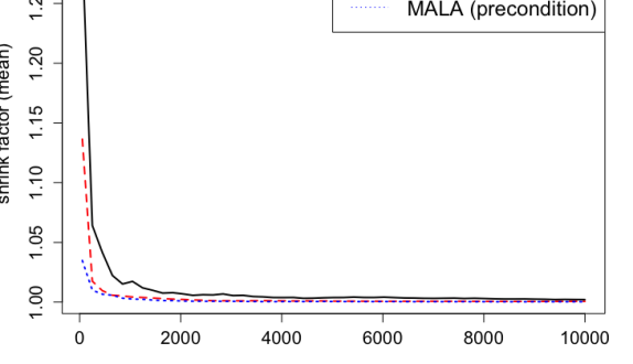
(a) $\theta_{1}$

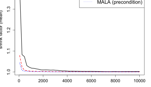
(b) $\theta_{2}$

(c) $\theta_{3}$

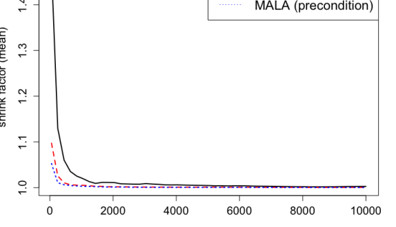
(d) $\theta_{4}$

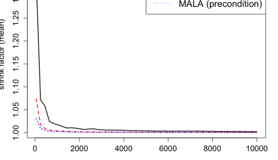
(e) $\theta_{5}$

Figure 1: Gelman–Rubin plots for each dimension of parameter vector $\theta$ in Bayesian quantile regression: mean.

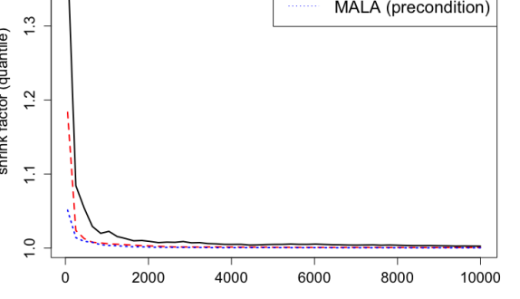
(a) $\theta_{1}$

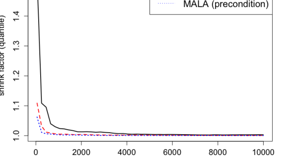
(b) $\theta_{2}$

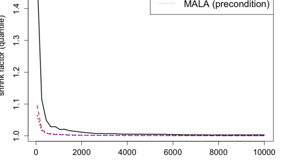
(c) $\theta_{3}$

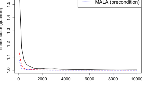
(d) $\theta_{4}$

(e) $\theta_{5}$

Figure 2: Gelman–Rubin plots for each dimension of parameter vector $\theta$ in Bayesian quantile regression: $97.5\%$ quantile.

7.1 Set up

We carry out experiment using the Bayesian quantile regression example, where the corresponding Bayesian posterior is given by

$$\pi_{n}(\theta\,|\,X^{(n)})\propto\exp\bigg{\{}-\sum_{i=1}^{n}(Y_{i}-\widetilde{X}_{i}^{T}\theta)\cdot\big{(}\tau-\mathbb{1}(Y_{i}<\widetilde{X}_{i}^{T}\theta)\big{)}\bigg{\}}\,\pi(\theta),\ \ \theta\in\mathbb{R}^{d}.$$

We choose the sample size $n=500$ and parameter dimension $d=5$. The covariates $\widetilde{X}$ is generated from a multivariate Gaussian distribution with zero mean and covariance matrix being chosen as a matrix whose diagonal elements are all $1$ and other elements are all $0.2$. We then generate a random error variable $e$ follows a Laplace distribution with location parameter being $0$ and scale parameter being $2$. The response variable $Y$ is then given by $Y=\widetilde{X}^{T}\theta^{\ast}+e$ with $\theta^{\ast}=(1,2,3,4,5)$. We consider the parameter space $\Theta=[-100,100]^{d}$ and the prior is chosen to be a uniform distribution over $\Theta$. We use three MCMC methods: MRW, MALA and MALA with a preconditioning matrix $n^{-1}\sum_{i=1}^{n}\widetilde{X}_{i}\widetilde{X}_{i}^{T}$ as suggested by Corollary 2.

7.2 Results

We use the Gelman–Rubin convergence diagnostic tool (Gelman and Rubin, 1992) to check the convergence of the Markov chains, and use their effective sample sizes to report the efficiency of the proposed MCMC algorithm. The Gelman–Rubin plots for each algorithm are given in Figure 1 and Figure 2, we can see MALA converges much faster than MRW and adding a preconditioning matrix to MALA can help to improve the convergence speed. More specifically, the number of iterations required for the MCMC procedure to have a shrink factor less than $1.01$ are $3434$ for MRW, $648$ for MALA and $449$ for preconditioned MALA. Moreover, for the effective sample size, the average required numbers of iterations for MRW to have a $300$ effective sample size for all dimensions is $6639$, while that is $1745$ for MALA and $1205$ for preconditioned MALA. In addition, the effective sample sizes of the Markov chain for each dimension of samples with a total number of $5000$ iterations are on average $(281,253,266,226,274)$ for MRW, $(1002,902,1447,887,1151)$ for MALA, and $(1561,1571,1244,1375,1690)$ for preconditioned MALA. We can see that MALA has much higher efficiency than MRW and adding a preconditioning matrix in MALA will further improve the sampling efficiency.

8 Conclusion and Discussion

In this paper, we studied the sampling complexity of Bayesian (pseudo-)posteriors using MALA under large sample size, covering cases where the posterior density is non-smooth and/or non-log-concave. A variant of MALA that includes a preconditioning matrix was also considered. While our analysis for the preconditioned MALA suggests an adaptive MALA with a data-driven preconditioning matrix may be preferable, its rigorous theoretical analysis may leave as our future work. When applying our main result to Bayesian inference, we mainly considered the Gibbs posterior, while similar analysis may carry over to other types of Bayesian pseudo-posterior, such as Bayesian empirical likelihood (Lazar, 2003), and we leave this for future research.

Appendix

We summarize some necessary notation and definitions in the appendix. We use $\mathbb{1}_{A}$ to denote the indicator function of a set $A$ so that $1_{A}(x)=1$ if $x\in A$ and zero otherwise. For two sequences $\{a_{n}\}$ and $\{b_{n}\}$, we use the notation $a_{n}\lesssim b_{n}$ and $a_{n}\gtrsim b_{n}$ to mean $a_{n}\leq Cb_{n}$ and $a_{n}\geq Cb_{n}$, respectively, for some constant $C>0$ independent of $n,d$. In addition, $a_{n}\asymp b_{n}$ means that both $a_{n}\lesssim b_{n}$ and $a_{n}\gtrsim b_{n}$ hold, and $a_{n}=\mathcal{O}(b_{n})$ if $a_{n}\lesssim b_{n}$; $a_{n}=\Theta(b_{n})$ if $a_{n}\asymp b_{n}$. When no ambiguity arises, for an absolutely continuous probability measure $\pi$, we also use $\pi$ to denote its density function (w.r.t. the Lebesgue measure). we use $\mathbb{N}(\mathcal{F},d_{n},\varepsilon)$ to denote the $\varepsilon$-covering number of $\mathcal{F}$ with respect to pseudo-metric $d_{n}$. Throughout, $C$, $c$, $C_{0}$, $c_{0}$, $C_{1}$, $c_{1}$, …are generically used to denote positive constants independent of $n,d$ whose values might change from one line to another.

Appendix A Proof of Main Results

A.1 Proof of Theorem 1

To prove Theorem 1, we introduce a notion of $s$-conductance profile, defined as

$$\Phi_{s}(v):=\inf\left\{\frac{\int_{S}T(x,S^{c})\mu(x)\,{\rm d}x}{\mu(S)-s}\,|\,S\subseteq\mathbb{R}^{d},s<\mu(S)\leq v\right\},$$

with $\mu$ and $T(\cdot,\cdot)$ being the stationary distribution and the Markov transition kernel of the considered Markov chain, respectively. Note that the $s$-conductance profile can be seen as an extension of the commonly used $s$-conductance considered in Lovász and Simonovits (1993b), which corresponds to $\Phi_{s}(\frac{1}{2})$. We will use the $s$-conductance profile to develop mixing time upper bound using Lemma 1 and Lemma 2.

Note that combined with Lemma 1, if the assumptions in Lemma 2 holds, we have

$$\tau_{\rm mix}(\varepsilon,\mu_{0}) \leq\frac{C}{\zeta}\,\int_{\frac{4}{M_{0}}}^{\frac{1}{2}}\frac{1}{v}\,{\rm d}v+\frac{C}{\zeta}\,\int_{\frac{4}{M_{0}}}^{\frac{1}{2}}\lambda^{-2}\psi^{-2}\frac{1}{v\log(1+\frac{1}{v})}\,{\rm d}v+\frac{C}{\zeta}\,\int_{\frac{1}{2}}^{\frac{4\sqrt{2}}{\varepsilon}}\lambda^{-2}\psi^{-2}\frac{1}{v}\,{\rm d}v$$ (12)

$$\leq\frac{C_{1}}{\zeta}\,\log M_{0}+\frac{C_{1}}{\zeta}\,\lambda^{-2}\psi^{-2}\log(\log M_{0})+\frac{C_{1}}{\zeta}\,\lambda^{-2}\psi^{-2}\log\frac{1}{\varepsilon},$$

where the last inequality follows equation (18) of Chen et al. (2020). Now it remains to verify the assumptions in Lemma 2. Fix a lazy parameter $\zeta\in(0,\frac{1}{2}]$. Consider a linear transformation $G:\mathbb{R}^{d}\to\mathbb{R}^{d}$ defined as $G(\theta)=\sqrt{n}\widetilde{I}^{-\frac{1}{2}}(\theta-\widehat{\theta})$, and let $\widetilde{\mu}_{k}=G_{\#}\mu_{k}$ denote the push forward measure of $G$ by $\mu_{k}$ for $k\in\mathbb{N}$ and $\widetilde{\pi}_{\rm loc}$ denote the push forward measure of $G$ by $\pi_{n}$. Then it holds that

$$M_{0}=\underset{A:\pi_{n}(A)>0}{\sup}\frac{\mu_{0}(A)}{\pi_{n}(A)}=\underset{A:\widetilde{\pi}_{\rm loc}(A)>0}{\sup}\frac{\widetilde{\mu}_{0}(A)}{\widetilde{\pi}_{\rm loc}(A)}.$$

Moreover, by the invariability of $\chi^{2}$ measure to linear transformation, we have $\chi^{2}(\mu_{k},\pi_{n})=\chi^{2}(\widetilde{\mu}_{k},\widetilde{\pi}_{\rm loc})$. Define

$$\widetilde{Q}(\xi,\cdot)=N_{d}(\xi-h\widetilde{I}^{\frac{1}{2}}\widetilde{\nabla}V_{n}(\widetilde{I}^{\frac{1}{2}}\xi),2h\,I_{d}),$$

and the corresponding Markov transition kernel

$$\widetilde{T}(\xi,\cdot)=\left[1-(1-\zeta)\cdot\int\widetilde{A}(\xi,y)\widetilde{Q}(\xi,y)\,{\rm d}y\right]\mathbb{1}_{\xi}(\cdot)+(1-\zeta)\cdot\widetilde{Q}(\xi,\cdot)\widetilde{A}(\xi,\cdot)$$

with

$$\widetilde{A}(\xi,y)=1\wedge\frac{\widetilde{\pi}_{\rm loc}(y)\widetilde{Q}(y,\xi)}{\widetilde{\pi}_{\rm loc}(\xi)\widetilde{Q}(\xi,y)}.$$

We have the following lemma.

Lemma 4.

For any $k\in\mathbb{N}$, $\widetilde{\mu}_{k}=G_{\#}\mu_{k}$ is the probability distribution obtained after $k$ steps of a Markov chain with transition kernel $\widetilde{T}$ and initial distribution $\widetilde{\mu}_{0}$.

It remains to calculate the mixing time of $\widetilde{\mu}_{k}$ converging to $\widetilde{\pi}_{\rm loc}$, which is equivalent to verify the assumptions in Lemma 2 for Markov transition kernel $\widetilde{T}(\xi,\cdot)$ with stationary distribution $\widetilde{\pi}_{\rm loc}$. Recall $K=\{x\,:\,\|\widetilde{I}^{-\frac{1}{2}}x\|\leq R\}$. By Condition A, firstly we have

$$\underset{\widetilde{\xi}\in B_{R}^{d}}{\sup}\big{|}V_{n}(\widetilde{I}^{\frac{1}{2}}\widetilde{\xi})-\frac{1}{2}{\widetilde{\xi}^{T}\widetilde{I}^{\frac{1}{2}}J\widetilde{I}^{\frac{1}{2}}\widetilde{\xi}}\big{|}=\underset{\xi\in K}{\sup}\big{|}V_{n}(\xi)-\frac{1}{2}{\xi^{T}J\xi}\big{|}=\widetilde{\varepsilon}\leq 0.04;$$

$$\underset{\widetilde{\xi}\in B_{R}^{d}}{\sup}\big{\|}\widetilde{I}^{\frac{1}{2}}\widetilde{\nabla}V_{n}(\widetilde{I}^{\frac{1}{2}}\xi)-\widetilde{I}^{\frac{1}{2}}J\widetilde{I}^{\frac{1}{2}}\xi\|=\underset{\xi\in K}{\sup}\big{\|}\widetilde{I}^{\frac{1}{2}}(\widetilde{\nabla}V_{n}(\xi)-J\xi)\|\leq\widetilde{\varepsilon}_{1}{|\kern-0.96873pt|\kern-0.96873pt|\widetilde{I}^{\frac{1}{2}}|\kern-0.96873pt|\kern-0.96873pt|}_{\scriptsize\rm op},$$

and $\widetilde{\pi}_{\rm loc}(\widetilde{\xi}\in B_{R/2}^{d})=\pi_{n}(\|\sqrt{n}\widetilde{I}^{-\frac{1}{2}}(\theta-\widehat{\theta})\|\leq R/2)\geq 1-\frac{h\rho_{1}\varepsilon^{2}}{M_{0}^{2}}$. We then verify the log-isoperimetric inequality in the following lemma.

Lemma 5.

Let $\widetilde{K}=B_{R/2}^{d}$, consider any measurable partition form $\widetilde{K}=S_{1}\cup S_{2}\cup S_{3}$ such that $\inf_{x\in S_{1},z\in S_{2}}\|x-z\|\geq t$, we have

$$\widetilde{\pi}_{\rm loc}|_{\widetilde{K}}(S_{3})\geq\frac{\sqrt{\rho_{1}}}{2}t\exp(-4\widetilde{\varepsilon})\min\{\widetilde{\pi}_{\rm loc}|_{\widetilde{K}}(S_{1}),\widetilde{\pi}_{\rm loc}|_{\widetilde{K}}(S_{2})\}\log^{\frac{1}{2}}\Big{(}1+\frac{1}{\min\{\widetilde{\pi}_{\rm loc}|_{\widetilde{K}}(S_{1}),\widetilde{\pi}_{\rm loc}|_{\widetilde{K}}(S_{2})\}}\Big{)}.$$

We then show that $\|\widetilde{T}(x,\cdot)-\widetilde{T}(y,\cdot)\|_{\rm TV}$ can be bounded with high probability in the following lemma.

Lemma 6.

There exists a set $E$ so that $\widetilde{\pi}_{\rm loc}(E)\geq 1-\frac{2\varepsilon^{2}h\rho_{1}}{M_{0}^{2}}$ and for any $x,z\in E$ with $\|x-z\|\leq\frac{\sqrt{2h}}{24}$, we have $\|\widetilde{T}(x,\cdot)-\widetilde{T}(z,\cdot)\|_{\rm TV}\leq\frac{17}{18}$.

Thus the first and second assumptions in Lemma 2 holds with $\lambda=\frac{\sqrt{\rho_{1}}}{2}\exp(-4\widetilde{\varepsilon})$ and $\psi=\frac{\sqrt{2h}}{24}$. Moreover, for the third assumption in Lemma 2, by $h\rho_{1}\leq c_{0}d^{-\frac{1}{3}}$ and $\widetilde{\varepsilon}\leq 0.04$, for small enough $c_{0}$, we have

$$\frac{2\varepsilon^{2}h\rho_{1}}{M_{0}^{2}}\leq\frac{\sqrt{2h}}{24}\frac{\sqrt{\rho_{1}}}{2}\exp(-4\widetilde{\varepsilon})\frac{\varepsilon^{2}}{256M_{0}^{2}}.$$

Thus all the assumptions in Lemma 2 are satisfied. The desired result then follows from equation (12).

A.2 Proof of Theorem 2

Without loss of generality, we can assume the learning rate $\alpha=1$, as otherwise we can take $\ell(X,\theta)=\alpha\cdot\ell(X,\theta)$. We only need to verify that the Assumptions in Theorem 1 holds for the Bayesian Gibbs posterior. We state the following Lemmas to verify Condition A.

Lemma 7.

Let $\kappa_{2}={\frac{\beta_{1}}{\gamma_{3}+\beta_{1}(1+\gamma_{4})+2\gamma_{0}-\gamma_{4}}}\wedge{\frac{1}{1+2\gamma+2\gamma_{2}+4\gamma_{0}}}\wedge{\frac{1}{2+2(\gamma+\gamma_{0}+\gamma_{1})}}$. Under Conditions B.1-B.4, if $d\leq c(\frac{n}{\log n})^{\kappa_{2}}$ for a small enough constant $c$, then there exist $(n,d)$-independent constants $c_{1},C,C_{1}$ so that it holds with probability at least $1-c_{1}n^{-2}$ that for any $\xi\in\mathbb{R}^{d}$ with $1\leq\|\xi\|\leq C\sqrt{n}$,

$$\Big{|}V_{n}(\xi)-\frac{\xi^{T}\mathcal{H}_{\theta^{*}}\xi}{2}\Big{|}\leq C_{1}\,\Big{(}d^{1+\gamma}\|\xi\|\frac{\log n}{\sqrt{n}}+d^{\gamma_{2}}\|\xi\|^{3}\frac{1}{\sqrt{n}}+d^{\frac{1+\gamma_{4}}{2}+\gamma_{2}}\|\xi\|^{2}\sqrt{\frac{\log n}{n}}$$

$$\qquad\qquad+d^{\frac{1+\gamma_{3}}{2}}\|\xi\|^{1+\beta_{1}}\frac{\sqrt{\log n}}{n^{\beta_{1}/2}}\Big{)};$$

$$\Big{\|}\widetilde{\nabla}V_{n}(\xi)-\mathcal{H}_{\theta^{*}}\xi\Big{\|}\leq C_{1}\,\Big{(}d^{1+\gamma}\frac{\log n}{\sqrt{n}}+d^{\gamma_{2}}\|\xi\|^{2}\frac{1}{\sqrt{n}}+d^{\frac{1+\gamma_{4}}{2}+\gamma_{2}}\|\xi\|\sqrt{\frac{\log n}{n}}$$

$$+d^{\frac{1+\gamma_{3}}{2}}\|\xi\|^{\beta_{1}}\frac{\sqrt{\log n}}{n^{\beta_{1}/2}}\Big{)}\text{ with }\widetilde{\nabla}V_{n}(\xi)=\frac{1}{\sqrt{n}}\sum_{i=1}^{n}g\Big{(}X_{i},\frac{\xi}{\sqrt{n}}+\widehat{\theta}\,\Big{)}-\frac{1}{\sqrt{n}}\nabla(\log\pi)\Big{(}\frac{\xi}{\sqrt{n}}+\widehat{\theta}\,\Big{)}.$$

We provide in the following lemma a tail inequality for the Gibbs posterior $\pi_{n}$.

Lemma 8.

Under Condition B.1-B.4. when $d\leq c\frac{n^{\kappa_{3}}}{\log n}$ for a small enough constant $c$, where

$$\kappa_{3} ={\frac{\beta_{1}}{1+\gamma_{3}+[(2\gamma_{0})\vee((1+\gamma_{0})(1+\beta_{1}))]}}\wedge{\frac{1}{3+\gamma_{0}+((2\gamma)\vee(\gamma_{4}+2\gamma_{2}+\gamma_{0})\vee(2\gamma_{2}+2\gamma_{0}))}}$$

$$\wedge{\frac{1}{1+2\gamma+6\gamma_{0}+4\gamma_{2}+\gamma_{4}}}\wedge{\frac{1}{2\gamma+2\gamma_{0}+2\gamma_{1}+(2\vee(1+\gamma_{4}))}},$$

then there exist $(n,d)$-independent constants $c_{1},c_{2},c_{3}$ so that it holds with probability at least $1-c_{1}n^{-2}$ that

$$\pi_{n}\Big{(}\sqrt{n}\|\widetilde{I}^{-\frac{1}{2}}(\theta-\widehat{\theta})\|\geq{|\kern-0.96873pt|\kern-0.96873pt|\widetilde{I}^{-\frac{1}{2}}|\kern-0.96873pt|\kern-0.96873pt|}_{\rm op}\vee\frac{3(\sqrt{d}+t)}{\sqrt{\lambda_{\min}(\widetilde{J})}}\Big{)}\leq\exp(-t^{2})+c_{2}\exp\big{(}-c_{3}n\,d^{-\gamma_{0}}(d^{-\gamma_{1}}\wedge d^{-2\gamma_{0}-2\gamma_{2}})\big{)},$$

where $\widetilde{J}=\widetilde{I}^{\frac{1}{2}}\mathcal{H}_{\theta^{*}}\widetilde{I}^{\frac{1}{2}}$.

By Condition B.1, we have ${|\kern-0.96873pt|\kern-0.96873pt|\mathcal{H}_{\theta^{*}}|\kern-0.96873pt|\kern-0.96873pt|}_{\rm op}\leq C\,d$ and ${|\kern-0.96873pt|\kern-0.96873pt|\mathcal{H}_{\theta^{*}}^{-1}|\kern-0.96873pt|\kern-0.96873pt|}_{\rm op}\leq C\,d^{\gamma_{0}}$. Moreover, since ${|\kern-0.96873pt|\kern-0.96873pt|\widetilde{I}^{-1}|\kern-0.96873pt|\kern-0.96873pt|}_{\rm op}{|\kern-0.96873pt|\kern-0.96873pt|\widetilde{I}|\kern-0.96873pt|\kern-0.96873pt|}_{\rm op}\leq C{|\kern-0.96873pt|\kern-0.96873pt|\mathcal{H}_{\theta^{*}}|\kern-0.96873pt|\kern-0.96873pt|}_{\rm op}{|\kern-0.96873pt|\kern-0.96873pt|\mathcal{H}_{\theta^{*}}^{-1}|\kern-0.96873pt|\kern-0.96873pt|}_{\rm op}$ and ${{|\kern-0.96873pt|\kern-0.96873pt|\widetilde{I}|\kern-0.96873pt|\kern-0.96873pt|}_{\rm op}{|\kern-0.96873pt|\kern-0.96873pt|(\widetilde{I}^{\frac{1}{2}}H_{\theta^{*}}\widetilde{I}^{\frac{1}{2}})^{-1}|\kern-0.96873pt|\kern-0.96873pt|}_{\rm op}}\leq C\,{|\kern-0.96873pt|\kern-0.96873pt|\mathcal{H}_{\theta^{*}}^{-1}|\kern-0.96873pt|\kern-0.96873pt|}_{\rm op}$, we can obtain that there exists constants $C_{2},C_{3}$ so that for any $R={|\kern-0.96873pt|\kern-0.96873pt|\widetilde{I}^{-\frac{1}{2}}|\kern-0.96873pt|\kern-0.96873pt|}_{\rm op}\vee\frac{3(\sqrt{d}+t)}{\sqrt{\lambda_{\min}(\widetilde{J})}}$ with $t\geq 0$, and set $K=\{x:\|\widetilde{I}^{-1/2}x\|\leq R\}$, we have $K\subseteq\{x\,:\,\|x\|\leq C_{2}d^{\frac{1+\gamma_{0}}{2}}+C_{3}td^{\frac{\gamma_{0}}{2}}\}$. Then by Lemma 7, for any $t=C_{1}\,(d^{\frac{\gamma_{5}}{2}}+\sqrt{\log n})$ (note that $\gamma_{5}\geq 1$), we can find a constant $c$ so that when $d\leq c\frac{n^{\kappa_{1}}}{\log n}$, we have

$${|\kern-0.96873pt|\kern-0.96873pt|\widetilde{I}|\kern-0.96873pt|\kern-0.96873pt|}_{\rm op}\,R^{2}\underset{\xi\in K}{\sup}\|\widetilde{\nabla}V_{n}(\xi)-\mathcal{H}_{\theta^{*}}\xi\Big{\|}^{2}\leq d^{\frac{1}{3}}.$$

So in this case the step size parameter $\widetilde{h}=h/n$ in Theorem 1 satisfies

$$h\leq c_{0}\cdot\bigg{[}\rho_{2}\Big{(}2d^{\frac{1}{3}}+d^{\frac{1}{4}}\big{(}\log\frac{M_{0}d\kappa}{\varepsilon}\big{)}^{\frac{1}{4}}+\big{(}\log\frac{M_{0}d\kappa}{\varepsilon}\big{)}^{\frac{1}{2}}\Big{)}\bigg{]}^{-1}$$

Then by the assumption $\log(\frac{M_{0}\rho_{2}}{\varepsilon\rho_{1}})\leq C_{1}\,(d^{\gamma_{5}}+\log n)$, using Lemma 8 and $d\leq c\frac{n^{\kappa_{1}}}{\log n}$, we can obtain that there exists a large enough $C_{1}$ so that for $t=C_{1}\,(d^{\frac{\gamma_{5}}{2}}+\sqrt{\log n})$, $\pi_{n}(K)=\pi_{n}\Big{(}\sqrt{n}\|\widetilde{I}^{-\frac{1}{2}}(\theta-\widehat{\theta})\|\geq{|\kern-0.96873pt|\kern-0.96873pt|\widetilde{I}^{-\frac{1}{2}}|\kern-0.96873pt|\kern-0.96873pt|}_{\rm op}\vee\frac{3(\sqrt{d}+t)}{\sqrt{\lambda_{\min}(\widetilde{J})}}\Big{)}\geq 1-\frac{h\rho_{1}\varepsilon^{2}}{M_{0}^{2}}$. So the Assumptions in Theorem 1 are satisfied.

Appendix B Proof of Lemmas for Theorem 1

B.1 Proof of Lemma 1

Fix an arbitrary $\varepsilon>0$. Suppose $\tau_{\rm mix}(\sqrt{2}\varepsilon,\mu_{0})>N=\int_{\frac{4}{M_{0}}}^{\frac{1}{2}}\frac{16{\rm d}v}{\zeta\cdot v\Phi_{s}^{2}(v)}+\int_{\frac{1}{2}}^{\frac{4}{\varepsilon}}\frac{64{\rm d}v}{\zeta\cdot v\Phi_{s}^{2}(\frac{1}{2})}$. Then for any $k\leq N$, $\chi^{2}(\mu_{k},\mu)>2\varepsilon^{2}$, where we use $\chi^{2}(\cdot,\cdot)$ to denote the $\chi^{2}$ divergence, $\mu_{k}$ to denote the distribution in $k$ step of the Markov chain and $\mu\in\mathcal{P}(\mathbb{R}^{d})$ to denote the stationary distribution. Then we will prove by contradiction that if $N<\tau_{\rm mix}(\sqrt{2}\varepsilon,\mu_{0})$, then when $k=N$, $\chi^{2}(\mu_{k},\mu)\leq 2\varepsilon^{2}$, which oppositely implies $N\geq\tau_{\rm mix}(\sqrt{2}\varepsilon,\mu_{0})$. Our proof is based on the strategy used in Chen et al. (2020). We first introduce the following related notations. For a measurable set $S\subseteq\mathbb{R}^{d}$ and positive numbers $\varepsilon,M_{0}$ , the $(\varepsilon,M_{0})$-spectral gap for the set $S$ is defined as

$$\Lambda_{\varepsilon,M_{0}}(S):=\inf_{g\in c_{\varepsilon,M_{0}}^{+}(S)}\frac{\mathcal{E}(g,g)}{\operatorname{Var}_{\mu}(g)}$$

where

$$c_{\varepsilon,M_{0}}^{+}(S):=\left\{g\in L_{2}\left(\mu\right)\mid\operatorname{supp}(g)=\{x\,:\,g(x)>0\}\subset S,\,0\leq g\leq M_{0},\,{\rm Var}_{\mu}(g)\geq\varepsilon^{2}\right\},$$

and

$$\mathcal{E}(g,g)=\frac{1}{2}\int(g(x)-g(y))^{2}T(x,y)\mu(x)\,{\rm d}y\,{\rm d}x,$$

with $T(x,y)$ denoting the Markov transition kernel. Moreover, we can define the $(\varepsilon,M_{0},s)$-spectral profile $\overline{\Lambda}_{s}^{\varepsilon,M_{0}}$ as

$$\overline{\Lambda}_{s}^{\varepsilon,M_{0}}(v):=\underset{\mu(S)\in(s,v]}{\inf}\Lambda_{\varepsilon,M_{0}}(S).$$

Define the ratio density

$$h_{k}(x)=\frac{\mu_{k}(x)}{\mu(x)}.$$

Note that

$$\mathbb{E}_{\mu}[h_{k}]=1\quad\text{and}\quad\chi^{2}(\mu_{k},\mu)={\rm Var}_{\mu}(h_{k}),$$

and $h_{k}(x)\leq M_{0}$ for all $k\geq 0$ (see for example, equation (64) of Chen et al. (2020)). By tracking the proof of Lemma 11 in Chen et al. (2020), it suffices to show that for any $k\leq N$,

$$2\,\mathcal{E}(h_{k},h_{k})\geq{\rm Var}_{\mu}(h_{k})\overline{\Lambda}^{\varepsilon,M_{0}}_{s}\Big{(}\frac{4}{{\rm Var}_{\mu}(h_{k})}\Big{)},$$ (13)

and

$$\overline{\Lambda}_{s}^{\varepsilon,M_{0}}(v)\geq\left\{\begin{array}[]{ll}\frac{\Phi_{s}^{2}(v)}{16}&\text{ for all }v\in\left[\frac{4}{M_{0}},\frac{1}{2}\right];\\ \frac{\Phi_{s}^{2}\left(\frac{1}{2}\right)}{64}&\text{ for all }v\in(\frac{1}{2},\infty),\end{array}\right.$$ (14)

with $s=\frac{\varepsilon^{2}}{16M_{0}^{2}}$. We first prove claim (13). Define $\gamma_{k}=\frac{{\rm Var}_{\mu}(h_{k})}{4\mathbb{E}_{\mu}[h_{k}]}=\frac{{\rm Var}_{\mu}(h_{k})}{4}$. Then for any $k\leq N$,

$$\operatorname{Var}_{\mu}\left((h_{k}-\gamma_{k})_{+}\right) =\mathbb{E}_{\mu}\left[((h_{k}-\gamma_{k})_{+})^{2}\right]-(\mathbb{E}_{\mu}\left[(h_{k}-\gamma_{k})_{+}\right])^{2}$$

$$\overset{(i)}{\geq}\mathbb{E}_{\mu}[h_{k}^{2}]-2\gamma_{k}\mathbb{E}_{\mu}[h_{k}]-(\mathbb{E}_{\mu}[h_{k}])^{2}$$

$$=\operatorname{Var}_{\mu}(h_{k})-2\gamma_{k}\mathbb{E}_{\mu}[h_{k}]$$

$$=\frac{1}{2}\operatorname{Var}_{\mu}(h_{k})\geq\varepsilon^{2},$$

where $(x)_{+}=\max\{0,x\}$, $(i)$ is due to $((a-b)_{+})^{2}\leq a^{2}-2ab$, $(a-b)_{+}\leq a$, and the last inequality is due to the assumption that $N<\tau_{\rm mix}(\sqrt{2}\varepsilon,\mu_{0})$; moreover, since for any $x\in\mathbb{R}^{d}$, $0\leq h_{k}(x)\leq M_{0}$, we can get $(h_{k}-\gamma_{k})_{+}\in c_{\varepsilon,M_{0}}^{+}(\{h_{k}>\gamma_{k}\})$, which leads to

$$\mathcal{E}(h_{k},h_{k})\overset{(ii)}{\geq}\mathcal{E}((h_{k}-\gamma_{k})_{+},(h_{k}-\gamma_{k})_{+})\geq\operatorname{Var}_{\mu}\left((h_{k}-\gamma_{k})_{+}\right)\cdot\inf_{f\in c_{\varepsilon,M_{0}}^{+}(\{h_{k}>\gamma_{k}\})}\frac{\mathcal{E}(f,f)}{\operatorname{Var}_{\mu}(f)},$$ (15)

where $(ii)$ follows from the fact that $(a-b)^{2}=(a-c-(b-c))^{2}\geq((a-c)_{+}-(b-c)_{+})^{2}$. Furthermore, We have for any $k\leq N$,

$$M_{0}^{2}\,\mu(h_{k}\geq\gamma_{k})\geq\mathbb{E}_{\mu}[((h_{k}-\gamma_{k})_{+})^{2}]\geq\operatorname{Var}_{\mu}\left((h_{k}-\gamma_{k})_{+}\right)\geq\frac{1}{2}\operatorname{Var}_{\mu}(h_{k})\geq\varepsilon^{2}.$$

On the other hand, by applying Markov’s inequality, we also have

$$\mu(h_{k}\geq\gamma_{k})\leq\frac{\mathbb{E}_{\mu}[h_{k}]}{\gamma_{k}}=\frac{4}{{\rm Var}_{\mu}(h_{k})}.$$

Thus by equation (15), we can get for $s=\frac{\varepsilon^{2}}{16M_{0}^{2}}$,

$$\mathcal{E}(h_{k},h_{k})\geq\frac{1}{2}\operatorname{Var}_{\mu}(h_{k})\overline{\Lambda}_{s}^{\varepsilon,M_{0}}\Big{(}\frac{4}{{\rm Var}_{\mu}(h_{k})}\Big{)}.$$

Then we prove claim (14). For $v\in\big{[}\frac{4}{M_{0}},\frac{1}{2}\big{]}$, fix any $A\subset\mathbb{R}^{d}$ with $s<\mu(A)\leq v$ and $g\in c^{+}_{\frac{\varepsilon}{2},M_{0}}(A)$. Then by

$$\mathbb{E}_{\mu}\Big{[}\int(g^{2}(x)-g^{2}(y))_{+}T(x,y)\,{\rm d}y\Big{]}$$

$$=\mathbb{E}_{\mu}\Big{[}\int(g^{2}(x)-g^{2}(y))\mathbb{1}(g^{2}(x)>g^{2}(y))T(x,y)\,{\rm d}y\Big{]}$$

$$=\mathbb{E}_{\mu}\Big{[}\int\int_{0}^{+\infty}\mathbb{1}(g^{2}(y)\leq t<g^{2}(x))\,{\rm d}t\,T(x,y)\,{\rm d}y\Big{]}$$

$$=\int_{0}^{+\infty}\mathbb{E}_{\mu}\Big{[}\int\mathbb{1}(g^{2}(y)\leq t<g^{2}(x))T(x,y)\,{\rm d}y\Big{]}\,{\rm d}t,$$

let $H_{t}=\{x\in\mathbb{R}^{d}\,:\,g^{2}(x)>t\}$, we have

$$\int\int|g^{2}(x)-g^{2}(y)|T(x,y)\mu(x)\,{\rm d}x\,{\rm d}y$$

$$\geq\int\int(g^{2}(x)-g^{2}(y))_{+}T(x,y)\mu(x)\,{\rm d}x\,{\rm d}y$$

$$=\int_{0}^{+\infty}\mathbb{E}_{\mu}\Big{[}\int\mathbb{1}(g^{2}(y)\leq t<g^{2}(x))T(x,y)\,{\rm d}y\Big{]}\,{\rm d}t$$

$$=\int_{0}^{+\infty}\int_{x\in H_{t}}T(x,H_{t}^{c})\mu(x)\,{\rm d}x\,{\rm d}t.$$

Let $t^{*}=\sup\{t\geq 0:\mu(H_{t})>s\}$, note that $t^{*}$ always exists as otherwise, $\mu(g(x)=0)\geq 1-s$ and thus ${\rm Var}_{\mu}(g)\leq M_{0}^{2}s=\frac{\varepsilon^{2}}{16}$, which is contradictory to the requirement that ${\rm Var}_{\mu}(g)\geq\frac{\varepsilon^{2}}{4}$. Then

$$\int\int|g^{2}(x)-g^{2}(y)|T(x,y)\mu(x)\,{\rm d}x\,{\rm d}y$$

$$\geq\int_{0}^{t^{*}}\int_{x\in H_{t}}T(x,H_{t}^{c})\mu(x)\,{\rm d}x\,{\rm d}t+\int_{t^{*}}^{+\infty}\int_{x\in H_{t}}T(x,H_{t}^{c})\mu(x)\,{\rm d}x\,{\rm d}t$$

$$\geq\int_{0}^{t^{*}}(\mu(H_{t})-s)\,{\rm d}t\cdot\Phi_{s}(\mu(A))$$

$$=\Big{(}\mathbb{E}_{\mu}[g^{2}]-\int_{t^{*}}^{M_{0}^{2}}\mu(H_{t})\,{\rm d}t-st^{*}\Big{)}\cdot\Phi_{s}(\mu(A))$$

$$\overset{(ii)}{\geq}\Big{(}\mathbb{E}_{\mu}[g^{2}]-\frac{\varepsilon^{2}}{8}\Big{)}\cdot\Phi_{s}(\mu(A))$$

$$\overset{(iii)}{\geq}\frac{1}{2}\mathbb{E}_{\mu}[g^{2}]\Phi_{s}(\mu(A)),$$

where $(ii)$ uses the fact that $t^{*}\leq M_{0}^{2}$ and when $t>t^{*}$, $\mu(H_{t})\leq s=\frac{\varepsilon^{2}}{16M_{0}^{2}}$ and $(iii)$ uses $\mathbb{E}_{\mu}[g^{2}]\geq{\rm Var}_{\mu}(g)\geq\frac{\varepsilon^{2}}{4}$. Moreover, since

$$\int\int|g^{2}(x)-g^{2}(y)|T(x,y)\mu(x)\,{\rm d}x\,{\rm d}y$$

$$\leq\sqrt{\int\int(g(x)-g(y))^{2}T(x,y)\mu(x)\,{\rm d}x\,{\rm d}y}\cdot\sqrt{\int\int(g(x)+g(y))^{2}T(x,y)\mu(x)\,{\rm d}x\,{\rm d}y}$$

$$\leq\sqrt{2\mathcal{E}(g,g)}\cdot\sqrt{\int\int(2g^{2}(x)+2g^{2}(y))T(x,y)\mu(x)\,{\rm d}x\,{\rm d}y}$$

$$=\sqrt{2\,\mathcal{E}(g,g)}\cdot\sqrt{4\,\mathbb{E}_{\mu}[g^{2}]},$$

we have

$$\qquad\frac{1}{2}\mathbb{E}_{\mu}[g^{2}]\cdot\Phi_{s}(\mu(A))\leq\sqrt{2\,\mathcal{E}(g,g)}\cdot\sqrt{4\,\mathbb{E}_{\mu}[g^{2}]}$$

$$\Rightarrow\frac{\mathcal{E}(g,g)}{\operatorname{Var}_{\mu}(g)}\geq\frac{\Phi^{2}_{s}(\mu(A))}{16}.$$

Taking infimum over $A\subset\mathbb{R}^{d}$ with $s<\mu(A)\leq v$ and $g\in c^{+}_{\frac{\varepsilon}{2},M_{0}}(A)$, we have

$$\overline{\Lambda}_{s}^{\varepsilon,M_{0}}(v)\geq\ \overline{\Lambda}_{s}^{\frac{\varepsilon}{2},M_{0}}(v)\geq\underset{s<\mu(A)\leq v}{\inf}\frac{\Phi_{s}^{2}(\mu(A))}{16}\geq\frac{\Phi_{s}^{2}(v)}{16}.$$ (16)

For the case $v>\frac{1}{2}$, consider any $A\subset\mathbb{R}^{d}$ with $\mu(A)>\frac{1}{2}$ and $g\in c^{+}_{\varepsilon,M_{0}}(A)$. Let $0\leq\gamma\leq M_{0}$ be the number such that

$$s<\mu(\{g>\gamma\})\vee\mu(\{g<\gamma\})\leq\frac{1}{2}.$$

$\gamma$ always exists as otherwise, there exists $0\leq\widetilde{\gamma}\leq M_{0}$ such that $\mu\{g=\widetilde{\gamma}\}\geq 1-2s$, which leads to ${\rm Var}_{\mu}(g)\leq\mathbb{E}_{\mu}[(g-\widetilde{\gamma})^{2}]\leq 2M_{0}^{2}s<\varepsilon^{2}$, and this causes contradiction. We first consider the case that $\mu(\{g>\gamma\})\wedge\mu(\{g<\gamma\})>s$. We have

$$\mathcal{E}(g,g)=\mathcal{E}((g-\gamma),(g-\gamma))\geq\mathcal{E}((g-\gamma)_{+},(g-\gamma)_{+})+\mathcal{E}((g-\gamma)_{-},(g-\gamma)_{-}).$$

Since for any function $h\geq 0$ with $\mu({\rm supp}(h))\leq\frac{1}{2}$, using Cauchy-Schwarz inequality, it holds that

$$\mathbb{E}_{\mu}[h^{2}]=\int_{x\in\rm supp(h)}h^{2}(x)\mu(x)dx\geq\frac{(\mathbb{E}_{\mu}[h])^{2}}{\mu({\rm supp}(h))}\geq 2\,\mathbb{(}E_{\mu}[h])^{2},$$

which leads to

$${\rm Var}_{\mu}(h)\geq\frac{1}{2}\mathbb{E}_{\mu}[h^{2}].$$

Since $\varepsilon^{2}\leq{\rm Var}_{\mu}(g)\leq\mathbb{E}_{\mu}[(g-\gamma)^{2}]$ and $\mathbb{E}_{\mu}[(g-\gamma)^{2}]=\mathbb{E}_{\mu}[(g-\gamma)_{+}^{2}]+\mathbb{E}_{\mu}[(g-\gamma)_{-}^{2}]$, w.l.o.g, we can assume $\mathbb{E}_{\mu}[(g-\gamma)_{+}^{2}]\geq\frac{\mathbb{E}_{\mu}[(g-\gamma)^{2}]}{2}\geq\frac{\varepsilon^{2}}{2}$. Then taking $h=(g-\gamma)_{+}$, we can obtain

$$\mathcal{E}(g,g) \geq\mathcal{E}((g-\gamma)_{+},(g-\gamma)_{+})$$ (17)

$$\geq\mathbb{E}_{\mu}[(g-\gamma)^{2}_{+}]\cdot\frac{\mathcal{E}((g-\gamma)_{+},(g-\gamma)_{+})}{2\,{\rm Var}_{\mu}((g-\gamma)_{+})}$$

$$\overset{(i)}{\geq}\frac{1}{4}{\rm Var}_{\mu}(g)\cdot\underset{\mu(S)\in(s,\frac{1}{2}]}{\inf}\underset{f\in c^{+}_{\frac{\varepsilon}{2},M_{0}}(S)}{\inf}\frac{\mathcal{E}(f,f)}{{\rm Var}_{\mu}(f)}$$

$$\overset{(ii)}{\geq}\frac{1}{64}{\rm Var}_{\mu}(g)\Phi_{s}^{2}(\frac{1}{2}),$$

where $(i)$ uses $\mathbb{E}_{\mu}[(g-\gamma)_{+}^{2}]\geq\frac{\mathbb{E}_{\mu}[(g-\gamma)^{2}]}{2}\geq\frac{{\rm Var}_{\mu}(g)}{2}$ and ${\rm Var}_{\mu}((g-\gamma)_{+})\geq\frac{1}{2}\mathbb{E}_{\mu}[(g-\gamma)^{2}_{+}]\geq\frac{\varepsilon^{2}}{4}$, and $(ii)$ uses (16). Then we consider the case that $\mu(\{g>\gamma\})\wedge\mu(\{g<\gamma\})\leq s<\mu(\{g>\gamma\})\vee\mu(\{g<\gamma\})$. W.l.o.g, we can assume $\mu(\{g>\gamma\})>s$. Then we can obtain

$$\mathbb{E}_{\mu}[(g-\gamma)_{+}^{2}] =\mathbb{E}_{\mu}[(g-\gamma)^{2}]-\mathbb{E}_{\mu}[(g-\gamma)_{-}^{2}]$$

$$\geq\mathbb{E}_{\mu}[(g-\gamma)^{2}]-M_{0}^{2}s=\mathbb{E}_{\mu}[(g-\gamma)^{2}]-\frac{\varepsilon^{2}}{8}\geq\frac{\mathbb{E}_{\mu}[(g-\gamma)^{2}]}{2},$$

where the last inequality is due to $\mathbb{E}_{\mu}[(g-\gamma)^{2}]\geq{\rm Var}_{\mu}(g)\geq\varepsilon^{2}$. We can then obtain the desired result by taking infimum over $A\subset\mathbb{R}^{d}$ with $\mu(A)>\frac{1}{2}$ and $g\in c^{+}_{\varepsilon,M_{0}}(A)$ in (17).

B.2 Proof of Lemma 2

The proof follows from the standard conductance argument in Chewi et al. (2021); Belloni and Chernozhukov (2009); Dwivedi et al. (2019); Chen et al. (2020). Let $s=\frac{\varepsilon^{2}}{16M_{0}^{2}}$, and let $S$ be any measurable set of $\mathbb{R}^{d}$ with $s\leq\mu(S)\leq v\leq\frac{1}{2}$. Define the following subsets:

$$S_{1}:=\{x\in S|T(x,S^{c})\leq\frac{1}{36}\},$$

$$S_{2}:=\{x\in S^{c}|T(x,S)\leq\frac{1}{36}\},$$

$$S_{3}:=(S_{1}\cup S_{2})^{c},$$

Then same as the analysis in Chewi et al. (2021), if $\mu(S_{1})\leq\mu(S)/2$ or $\mu(S_{2})<\mu(S^{c})/2$, then by the fact that $\mu$ is stationary w.r.t the transition kernel $T$, we have

$$\int_{S}T(x,S^{c})\mu(x)\,{\rm d}x =\int T(x,S)\mu(x)\,{\rm d}x-\int_{S}T(x,S)\mu(x)\,{\rm d}x$$

$$=\int_{S^{c}}T(x,S)\mu(x)\,{\rm d}x\geq\frac{1}{36}\cdot\max\{\mu(S\cap S_{1}^{c}),\mu(S^{c}\cap S_{2}^{c})\}$$

$$\geq\frac{\mu(S)}{72}.$$

Then when $\mu(S_{1})\wedge\mu(S_{2})\geq\frac{\mu(S)}{2}$, consider $x\in E\cap S_{1}$ and $z\in E\cap S_{2}$, then $\|T_{x}-T_{z}\|_{\scriptsize\rm TV}\geq T(z,S^{c})-T(x,S^{c})\geq\frac{17}{18}$, thus $\|x-z\|\geq\psi$, which implies that $\inf_{x\in E\cap S_{1},z\in E\cap S_{2}}\|x-z\|\geq\psi$. Then take $S_{1}$ as $E\cap K\cap S_{1}$, $S_{2}$ as $E\cap K\cap S_{2}$ in the log-isoperimetric inequality of $\mu|_{K}$, we can obtain that

$$\mu|_{K}(((E\cap K\cap S_{1})\cup(E\cap K\cap S_{2}))^{c}) \geq\lambda\cdot\psi\cdot\min\{\mu|_{K}(E\cap K\cap S_{1}),\mu|_{K}(E\cap K\cap S_{2})\}$$

$$\cdot\log^{\frac{1}{2}}\Big{(}1+\frac{1}{\min\{\mu|_{K}(E\cap K\cap S_{1}),\mu|_{K}(E\cap K\cap S_{2})\}}\Big{)}$$

$$\geq\lambda\cdot\psi\cdot\min\{\mu(E\cap K\cap S_{1}),\mu(E\cap K\cap S_{2})\}$$

$$\cdot\log^{\frac{1}{2}}\Big{(}1+\frac{1}{\min\{\mu(E\cap K\cap S_{1}),\mu(E\cap K\cap S_{2})\}}\Big{)},$$

where the last inequality is due to the fact that the function $x\log^{\frac{1}{2}}(1+\frac{1}{x})$ is an increasing function. W.l.o.g, we can assume $\mu(E\cap K\cap S_{1})\leq\mu(E\cap K\cap S_{2})$, then by $((E\cap K\cap S_{1})\cup(E\cap K\cap S_{2}))^{c}\subseteq E^{c}\cup K^{c}\cup S_{3}$ and $\mu(E^{c})\leq(\lambda\psi\wedge 1)\frac{\varepsilon^{2}}{256M_{0}^{2}}=\frac{(\lambda\psi\wedge 1)s}{16}$, $\mu(K^{c})\leq\frac{(\lambda\psi\wedge 1)s}{16}$, we can obtain

$$\mu(S_{3})+\frac{16\lambda\psi s}{127}$$

$$\geq\mu(S_{3})+\frac{\mu(K^{c})+\mu(E^{c})}{\mu(K)}$$

$$\geq\mu|_{K}(((E\cap K\cap S_{1})\cup(E\cap K\cap S_{2}))^{c})$$

$$\geq\lambda\cdot\psi\cdot\mu(E\cap K\cap S_{1})\cdot\log^{\frac{1}{2}}\Big{(}1+\frac{1}{\mu(E\cap K\cap S_{1})}\Big{)},$$

$$\overset{\rm{(i)}}{\geq}\lambda\cdot\psi\cdot\big{(}\frac{\mu(S)}{4}+\frac{s}{4}-\frac{s}{8}\big{)}\log^{\frac{1}{2}}\Big{(}1+\frac{1}{\frac{\mu(S)}{4}+\frac{s}{4}-\frac{s}{8}\big{)}}\Big{)}$$

$$\geq\lambda\cdot\psi\cdot\frac{\mu(S)}{4}\log^{\frac{1}{2}}\Big{(}1+\frac{4}{\mu(S)}\Big{)},$$

where (i) uses $\mu(E\cap K\cap S_{1})\geq\mu(S_{1})-\mu(E^{c})-\mu(K^{c})$, $\mu(S_{1})\geq\frac{\mu(S)}{2}\geq\frac{s}{2}$ and the function $x\log^{\frac{1}{2}}(1+\frac{1}{x})$ is an increasing function. Then by $\mu(S)\geq s$, we can obtain

$$\mu(S_{3})\geq\lambda\cdot\psi\cdot\frac{\mu(S)}{9}\log^{\frac{1}{2}}\Big{(}1+\frac{4}{\mu(S)}\Big{)},$$

hence

$$\int_{S}T(x,S^{c})\mu(x)\,{\rm d}x \geq\frac{1}{2}\left(\int_{S}T(x,S^{c})\mu(x)\,{\rm d}x+\int_{S^{c}}T(x,S)\mu(x)\,{\rm d}x\right)$$

$$\geq\frac{1}{72}\mu(S_{3})\geq\frac{\lambda\cdot\psi}{648}\cdot{\mu(S)}\log^{\frac{1}{2}}\Big{(}1+\frac{4}{\mu(S)}\Big{)},$$

which leads to

$$\frac{\int_{S}T(x,S^{c})\mu(x)\,{\rm d}x}{\mu(S)}\geq\frac{\lambda\cdot\psi}{648}\cdot\log^{\frac{1}{2}}\Big{(}1+\frac{4}{\mu(S)}\Big{)}\geq\frac{\lambda\cdot\psi}{648}\cdot\log^{\frac{1}{2}}\Big{(}1+\frac{1}{v}\Big{)}.$$

Then combining with the result for the first case, we can obtain a lower bound of

$$\frac{1}{72}\,\min\Big{\{}1,\frac{\lambda\cdot\psi}{9}\sqrt{\log\big{(}1+\frac{1}{v}\big{)}}\Big{\}}$$

on $s$-conductance profile $\Phi_{s}(v)$ with $s=\frac{\varepsilon^{2}}{16M_{0}^{2}}$.

B.3 Proof of Lemma 4

Recall the transition kernel associated with $\mu_{k}$,

$$T(\theta,\cdot)=\left[1-(1-\zeta)\cdot\int A(\theta,y)Q(\theta,y)\,{\rm d}y\right]\delta_{\theta}(\cdot)+(1-\zeta)\cdot Q(\theta,\cdot)A(\theta,\cdot)$$

with

$$A(\theta,y)=1\wedge\frac{\pi_{n}(y)Q(y,\theta)}{\pi_{n}(\theta)Q(\theta,y)};\quad Q(\theta,\cdot)=N_{d}\Big{(}\theta-\frac{h}{\sqrt{n}}\widetilde{I}\widetilde{\nabla}V_{n}\big{(}\sqrt{n}(\theta-\widehat{\theta})\big{)},\frac{2h}{n}\,\widetilde{I}\Big{)}.$$

Then given $\xi\in\mathbb{R}^{d}$, the distribution of $G_{\#}T(\xi,\cdot)$ is

$$T^{*}(\theta,z)$$

$$=\left[1-(1-\zeta)\cdot\int N_{d}(\sqrt{n}\widetilde{I}^{-\frac{1}{2}}(\theta-\widehat{\theta})-h\widetilde{I}^{\frac{1}{2}}\widetilde{\nabla}V_{n}\big{(}\sqrt{n}(\theta-\widehat{\theta})),2hI_{d}\big{)}A\big{(}\theta,\widehat{\theta}+\widetilde{I}^{\frac{1}{2}}\frac{z}{\sqrt{n}}\big{)}\,{\rm d}z\right]\delta_{\theta}\Big{(}\widehat{\theta}+\widetilde{I}^{\frac{1}{2}}\frac{z}{\sqrt{n}}\Big{)}$$

$$+(1-\zeta)\cdot N_{d}(\sqrt{n}\widetilde{I}^{-\frac{1}{2}}(\theta-\widehat{\theta})-h\widetilde{I}^{\frac{1}{2}}\widetilde{\nabla}V_{n}\big{(}\sqrt{n}(\theta-\widehat{\theta})),2hI_{d}\big{)}A\big{(}\theta,\widehat{\theta}+\widetilde{I}^{\frac{1}{2}}\frac{z}{\sqrt{n}}\big{)}.$$

Then by the fact that

$$\frac{Q\big{(}\widehat{\theta}+\widetilde{I}^{\frac{1}{2}}\frac{z}{\sqrt{n}},\widehat{\theta}+\widetilde{I}^{\frac{1}{2}}\frac{\xi}{\sqrt{n}}\big{)}}{Q\big{(}\widehat{\theta}+\widetilde{I}^{\frac{1}{2}}\frac{\xi}{\sqrt{n}},\widehat{\theta}+\widetilde{I}^{\frac{1}{2}}\frac{z}{\sqrt{n}}\big{)}} =\exp\left(-\frac{1}{4h}\left(\|\xi-z+h\widetilde{I}^{\frac{1}{2}}\widetilde{\nabla}V_{n}(\widetilde{I}^{\frac{1}{2}}z)\|^{2}-\|z-\xi+h\widetilde{I}^{\frac{1}{2}}\widetilde{\nabla}V_{n}(\widetilde{I}^{\frac{1}{2}}\xi)\|^{2}\right)\right)$$

$$=\frac{\widetilde{Q}(z,\xi)}{\widetilde{Q}(\xi,z)},$$

we have

$$T^{*}\Big{(}\widehat{\theta}+\widetilde{I}^{\frac{1}{2}}\frac{\xi}{\sqrt{n}},\cdot\Big{)}=\left[1-(1-\zeta)\cdot\int\widetilde{A}(\xi,y)\widetilde{Q}(\xi,y)\,{\rm d}y\right]\mathbb{1}_{\xi}(\cdot)+(1-\zeta)\cdot\widetilde{Q}({\xi},\cdot)\widetilde{A}(\xi,\cdot)=\widetilde{T}(\xi,\cdot).$$

Thus when $\widetilde{\mu}_{k-1}=G_{\#}\mu_{k-1}$, we have $\widetilde{\mu}_{k}=G_{\#}\mu_{k}$. Then combine with the fact that $\widetilde{\mu}_{0}=G_{\#}\mu_{0}$, we can obtain by induction that $\widetilde{\mu}_{k}=G_{\#}\mu_{k}$ for $k\in\mathbb{N}$.

B.4 Proof of Lemma 5

To begin with, we consider the following lemma stated in Chen et al. (2020).

Lemma 9.

(Lemma 16 of Chen et al. (2020)) Let $\gamma$ denote the density of the standard Gaussian distribution $\mathcal{N}\left(0,\sigma^{2}{I}_{d}\right)$, and let $\mu$ be a distribution with density $\mu=q\cdot\gamma$, where $q$ is a log-concave function. Then for any partition $S_{1},S_{2},S_{3}$ of $\mathbb{R}^{d}$, we have

$$\mu\left(S_{3}\right)\geq\frac{d\left(S_{1},S_{2}\right)}{2\sigma}\min\left\{\mu\left(S_{1}\right),\mu\left(S_{2}\right)\right\}\log^{\frac{1}{2}}\left(1+\frac{1}{\min\left\{\mu\left(S_{1}\right),\mu\left(S_{2}\right)\right\}}\right).$$

We first consider the case $\widetilde{J}=I_{d}$ where recall $\widetilde{J}=\widetilde{I}^{\frac{1}{2}}J\widetilde{I}^{\frac{1}{2}}$. Then define $\overline{\pi}=N(0,I_{d})|_{\widetilde{K}}$, by the fact that $\widetilde{K}=B_{R/2}^{d}$ is a convex set and $\mathbb{1}_{\widetilde{K}}$ is a log-concave function, using lemma 9, we can obtain that for any partition $S_{1},S_{2},S_{3}$ of ${\widetilde{K}}$, we have

$$\overline{\pi}\left(S_{3}\right)\geq\frac{d\left(S_{1},S_{2}\right)}{2}\min\left\{\overline{\pi}\left(S_{1}\right),\overline{\pi}\left(S_{2}\right)\right\}\log^{\frac{1}{2}}\left(1+\frac{1}{\min\left\{\overline{\pi}\left(S_{1}\right),\overline{\pi}\left(S_{2}\right)\right\}}\right).$$

Then recall $\widetilde{\pi}_{\rm loc}|_{\widetilde{K}}(\xi)=\frac{\mathbb{1}_{\widetilde{K}}\exp(-V_{n}(\widetilde{I}^{\frac{1}{2}}\xi))}{\int_{\widetilde{K}}\exp(-V_{n}(\widetilde{I}^{\frac{1}{2}}\xi)){\rm d}\xi}$, using the fact that $\underset{\widetilde{\xi}\in B_{R}^{d}}{\sup}\big{|}V_{n}(\widetilde{I}^{\frac{1}{2}}\widetilde{\xi})-\frac{1}{2}{\widetilde{\xi}^{T}\widetilde{J}\widetilde{\xi}}\big{|}=\widetilde{\varepsilon}\leq 0.04$, we can obtain that for any measurable set $S\subseteq\widetilde{K}$, we have

$$\exp(-2\widetilde{\varepsilon})\leq\frac{\widetilde{\pi}_{\rm loc}|_{\widetilde{K}}(S)}{\overline{\pi}(S)}=\frac{\int_{S\cap\widetilde{K}}\exp(-V_{n}(\widetilde{I}^{\frac{1}{2}}\xi)){\rm d}\xi\int_{K}\exp(-\frac{1}{2}\xi^{T}\xi){\rm d}\xi}{\int_{S\cap K}\exp(-\frac{1}{2}\xi^{T}\xi){\rm d}\xi\int_{K}\exp(-V_{n}(\widetilde{I}^{\frac{1}{2}}\xi)){\rm d}\xi}\leq\exp(2\widetilde{\varepsilon}).$$

Thus

$$\widetilde{\pi}_{\rm loc}|_{\widetilde{K}}(S_{3})\geq\exp(-2\widetilde{\varepsilon})\overline{\pi}(S_{3})$$ (18)

$$\geq\frac{d(S_{1},S_{2})}{2}\exp(-2\widetilde{\varepsilon})\min\left\{\overline{\pi}\left(S_{1}\right),\overline{\pi}\left(S_{2}\right)\right\}\log^{\frac{1}{2}}\left(1+\frac{1}{\min\left\{\overline{\pi}\left(S_{1}\right),\overline{\pi}\left(S_{2}\right)\right\}}\right)$$

$$\overset{(i)}{\geq}\frac{d(S_{1},S_{2})}{2}\exp(-4\widetilde{\varepsilon})\min\left\{\widetilde{\pi}_{\rm loc}|_{\widetilde{K}}\left(S_{1}\right),\widetilde{\pi}_{\rm loc}|_{\widetilde{K}}\left(S_{2}\right)\right\}\log^{\frac{1}{2}}\left(1+\frac{1}{\exp(-2\widetilde{\varepsilon})\min\left\{\widetilde{\pi}_{\rm loc}|_{\widetilde{K}}\left(S_{1}\right),\widetilde{\pi}_{\rm loc}|_{\widetilde{K}}\left(S_{2}\right)\right\}}\right)$$

$$\geq\frac{d(S_{1},S_{2})}{2}\exp(-4\widetilde{\varepsilon})\min\left\{\widetilde{\pi}_{\rm loc}|_{\widetilde{K}}\left(S_{1}\right),\widetilde{\pi}_{\rm loc}|_{\widetilde{K}}\left(S_{2}\right)\right\}\log^{\frac{1}{2}}\left(1+\frac{1}{\min\left\{\widetilde{\pi}_{\rm loc}|_{\widetilde{K}}\left(S_{1}\right),\widetilde{\pi}_{\rm loc}|_{\widetilde{K}}\left(S_{2}\right)\right\}}\right),$$

where $(i)$ uses the fact that $x\log^{\frac{1}{2}}(1+\frac{1}{x})$ is an increasing function. For the general case where $\widetilde{J}$ is not necessary an identity matrix, we can define $K^{\prime}=\widetilde{J}^{\frac{1}{2}}\widetilde{K}=\{x=\widetilde{J}^{\frac{1}{2}}y\,:\,y\in\widetilde{K}\}$, and $\lambda=\widetilde{J}^{\frac{1}{2}}\xi$, where $\xi$ is a random variable with density $\pi_{\rm loc}|_{\widetilde{K}}$. Thus $\lambda$ has a density

$$\pi_{\lambda}(\lambda)=\frac{\mathbb{1}_{K^{\prime}}(\lambda)\exp(-V_{n}(\widetilde{I}^{\frac{1}{2}}\widetilde{J}^{-\frac{1}{2}}\lambda))}{\int_{K^{\prime}}\exp(-V_{n}(\widetilde{I}^{\frac{1}{2}}J^{-\frac{1}{2}}\lambda)){\rm d}\lambda},$$

Moreover, for any $\lambda\in K^{\prime}$, it holds that

$$\big{|}V_{n}(\widetilde{I}^{\frac{1}{2}}\widetilde{J}^{-\frac{1}{2}}\lambda)-\frac{1}{2}\lambda^{T}\lambda\big{|}\leq\widetilde{\varepsilon}.$$

Then for any partition $S_{1},S_{2},S_{3}$ of $\widetilde{K}$, let

$$\widetilde{S_{1}}=\widetilde{J}^{\frac{1}{2}}S_{1};$$

$$\widetilde{S_{2}}=\widetilde{J}^{\frac{1}{2}}S_{2};$$

$$\widetilde{S_{3}}=\widetilde{J}^{\frac{1}{2}}S_{3}.$$

Then by the positive definiteness of $\widetilde{J}$, $(\widetilde{S_{1}},\widetilde{S_{2}},\widetilde{S_{3}})$ forms a partition for $K^{\prime}$, and

$$d(\widetilde{S_{1}},\widetilde{S_{2}})\geq\sqrt{\rho_{1}}\,d(S_{1},S_{2}).$$

Since $K^{\prime}$ is a convex set, by applying $\pi_{\lambda}$ to statement (18), we can obtain

$$\widetilde{\pi}_{\rm loc}|_{\widetilde{K}}(S_{3})=\pi_{\lambda}(\widetilde{S}_{3})\geq\frac{d(\widetilde{S}_{1},\widetilde{S}_{2})}{2}\exp(-4\widetilde{\varepsilon})\min\left\{\pi_{\lambda}(\widetilde{S}_{1}),\pi_{\lambda}(\widetilde{S}_{2})\right\}\log^{\frac{1}{2}}\bigg{(}1+\frac{1}{\min\left\{\pi_{\lambda}(\widetilde{S}_{1}),\pi_{\lambda}(\widetilde{S}_{2})\right\}}\bigg{)}$$

$$\geq\frac{\sqrt{\rho_{1}}}{2}d(S_{1},S_{2})\exp(-4\widetilde{\varepsilon})\min\left\{\pi_{\rm loc}|_{\widetilde{K}}\left(S_{1}\right),\pi_{\rm loc}|_{\widetilde{K}}\left(S_{2}\right)\right\}\log^{\frac{1}{2}}\left(1+\frac{1}{\min\left\{\widetilde{\pi}_{\rm loc}|_{\widetilde{K}}\left(S_{1}\right),\widetilde{\pi}_{\rm loc}|_{\widetilde{K}}\left(S_{2}\right)\right\}}\right).$$

Proof is completed.

B.5 Proof of Lemma 6

We first construct the high probability set $E$ as follows: let

$$r_{d}=\Big{(}\sqrt{c^{\prime}d\log\left(\frac{M_{0}^{2}}{\varepsilon^{2}h\rho_{1}}\right)}\rho_{2}^{2}\Big{)}\vee\Big{(}c^{\prime}\log\left(\frac{M_{0}^{2}}{\varepsilon^{2}h\rho_{1}}\right)\rho_{2}^{2}\Big{)},$$

and $\widetilde{J}=\widetilde{I}^{\frac{1}{2}}J\widetilde{I}^{\frac{1}{2}}$. We define $E=\{\xi\in B_{R/2}^{d}:\big{|}\xi^{T}\widetilde{J}^{3}\xi-{\rm tr}(\widetilde{J}^{2})\big{|}\leq r_{d}\}\cap\{\xi\in B_{R/2}^{d}:\big{|}\xi^{T}\widetilde{J}^{2}\xi-{\rm tr}(\widetilde{J})\big{|}\leq r_{d}/\rho_{2}\}$. By the choice of $h$, when $c_{0}$ is small enough, it holds that

$$h\leq\sqrt{c_{0}}\cdot\left\{\left({\rho_{2}}^{-\frac{1}{3}}(\rho_{2}^{2}d+r_{d})^{-\frac{1}{3}}\right)\wedge(r_{d})^{-\frac{1}{2}}\right\}.$$

Now we show that $E$ is indeed a high probability set in the following lemma. Note that all the following lemmas in this subsection are under Assumptions in Theorem 1.

Lemma 10.

Consider $E=\{\xi\in B_{R/2}^{d}:\big{|}\xi^{T}\widetilde{J}^{3}\xi-{\rm tr}(\widetilde{J}^{2})\big{|}\leq r_{d}\}\cap\{\xi\in B_{R/2}^{d}:\big{|}\xi^{T}\widetilde{J}^{2}\xi-{\rm tr}(\widetilde{J})\big{|}\leq r_{d}/\rho_{2}\}$. If $r_{d}=\Big{(}\sqrt{c^{\prime}d\log\left(\frac{M_{0}^{2}}{\varepsilon^{2}h\rho_{1}}\right)}\rho_{2}^{2}\Big{)}\vee\Big{(}c^{\prime}\log\left(\frac{M_{0}^{2}}{\varepsilon^{2}h\rho_{1}}\right)\rho_{2}^{2}\Big{)}$ for a sufficiently large enough constant $c^{\prime}$, then $\widetilde{\pi}_{\rm loc}(E)\geq 1-\frac{2\varepsilon^{2}h\rho_{1}}{M_{0}^{2}}$.

We now show that for any $x,z\in E$ with $\|x-z\|\leq\frac{\sqrt{2h}}{24}$, the total variation distance between $\widetilde{T}_{x}=\widetilde{T}(x,\cdot)$ and $\widetilde{T}_{z}=\widetilde{T}(z,\cdot)$ can be upper bounded by $\frac{17}{18}$. For any $x,z\in E$, we consider the following decomposition:

$$\|\widetilde{T}_{x}-\widetilde{T}_{z}\|_{TV}$$ (19)

$$=\frac{1}{2}\int|\widetilde{T}(x,y)-\widetilde{T}(z,y)|\,{\rm d}y$$

$$=\frac{1}{2}\widetilde{T}_{x}(\{x\})+\frac{1}{2}\widetilde{T}_{z}(\{z\})+\frac{1}{2}\int_{\mathbb{R}^{d}/\{x,z\}}|\widetilde{T}(x,y)-\widetilde{T}(z,y)|\,{\rm d}y$$

$$\leq\frac{1}{2}\widetilde{T}_{x}(\{x\})+\frac{1}{2}\widetilde{T}_{z}(\{z\})+\frac{1}{2}(1-\zeta)\cdot\int_{B_{R}^{d}}|\widetilde{Q}(x,y)\widetilde{A}(x,y)-\widetilde{Q}(z,y)\widetilde{A}(z,y)|\,{\rm d}y$$

$$\qquad+\frac{1}{2}(1-\zeta)\cdot\int_{\mathbb{(}B_{R}^{d})^{c}}\Big{(}\widetilde{Q}(x,y)\widetilde{A}(x,y)+\widetilde{Q}(z,y)\widetilde{A}(z,y)\Big{)}\,{\rm d}y,$$

Then for the third term in (19),

$$\int_{B_{R}^{d}}|\widetilde{Q}(x,y)\widetilde{A}(x,y)-\widetilde{Q}(z,y)\widetilde{A}(z,y)|\,{\rm d}y \leq\int_{B_{R}^{d}}\widetilde{Q}(x,y)(1-\widetilde{A}(x,y))\,{\rm d}y$$

$$+\int_{B_{R}^{d}}\widetilde{Q}(z,y)(1-\widetilde{A}(z,y))\,{\rm d}y+2\|\widetilde{Q}_{x}-\widetilde{Q}_{z}\|_{\scriptsize\rm TV},$$

where we use $\widetilde{Q}_{x}$ to denote $\widetilde{Q}(x,\cdot)$. Consider the proposal distribution of MALA for sampling from the Gaussian $\overline{\pi}:\,=N_{d}(0,\widetilde{J}^{-1})$,

$$Q^{\Delta}_{x}(\cdot)=Q^{\Delta}(x,\cdot)=N_{d}(x-h\widetilde{J}x,2hI_{d}).$$

Then $\|\widetilde{Q}_{x}-\widetilde{Q}_{z}\|_{\scriptsize\rm TV}\leq\|\widetilde{Q}_{x}-Q^{\Delta}_{x}\|_{\scriptsize\rm TV}+\|Q_{x}^{\Delta}-Q_{z}^{\Delta}\|_{\scriptsize\rm TV}+\|\widetilde{Q}_{z}-Q^{\Delta}_{z}\|_{\scriptsize\rm TV}$ can be upper bounded by Pinsker’s inequality, that is, for any $x\in B_{R}^{d}$,

$$\|\widetilde{Q}_{x}-Q^{\Delta}_{x}\|_{\scriptsize\rm TV}\leq\frac{1}{2}\sqrt{\frac{h^{2}\|\widetilde{I}^{\frac{1}{2}}\widetilde{\nabla}V_{n}(\widetilde{I}^{\frac{1}{2}}x)-\widetilde{J}x\|^{2}}{2h}}\leq\frac{\sqrt{h}\widetilde{\varepsilon}_{1}{|\kern-0.96873pt|\kern-0.96873pt|\widetilde{I}^{\frac{1}{2}}|\kern-0.96873pt|\kern-0.96873pt|}_{\rm op}}{2\sqrt{2}},$$

and for any $x,z\in B_{R}^{d}$

$$\|Q_{x}^{\Delta}-Q_{z}^{\Delta}\|_{\scriptsize\rm TV}\leq\frac{1}{2}\sqrt{\frac{\|(I-h\widetilde{J})(x-z)\|^{2}}{2h}}\leq\frac{\|x-z\|}{2\sqrt{2h}}.$$

For the term of $\int_{B_{R}^{d}}\widetilde{Q}(x,y)(1-\widetilde{A}(x,y))\,{\rm d}y$, we use Condition A by comparing $Q_{x}$ with $Q_{x}^{\Delta}$, leading to the following decomposition:

$$\int_{B_{R}^{d}}\widetilde{Q}(x,y)(1-\widetilde{A}(x,y))\,{\rm d}y$$

$$\leq\int_{B_{R}^{d}}\Big{|}\widetilde{Q}(x,y)-\frac{\widetilde{\pi}_{\rm loc}(y)\widetilde{Q}(y,x)}{\widetilde{\pi}_{\rm loc}(x)}\Big{|}\,{\rm d}y$$

$$\leq 2\|\widetilde{Q}_{x}-Q_{x}^{\Delta}\|_{\scriptsize\rm TV}+\underbrace{\int\left|Q^{\Delta}(x,y)-\frac{\overline{\pi}(y)Q^{\Delta}(y,x)}{\overline{\pi}(x)}\right|{\rm d}y}_{\rm(A)}+\underbrace{\int_{B_{R}^{d}}\left|\frac{\overline{\pi}(y)Q^{\Delta}(y,x)}{\overline{\pi}(x)}-\frac{\widetilde{\pi}_{\rm loc}(y)\widetilde{Q}(y,x)}{\widetilde{\pi}_{\rm loc}(x)}\right|\,{\rm d}y}_{\rm(B)}.$$

We then state the following lemma for bounding the term (A).

Lemma 11.

Consider the choice of (rescaled) step size $h$ in Theorem 1, then when $c_{0}$ is small enough and $x\in E$, it holds that

$$\int\left|Q^{\Delta}(x,y)-\frac{\overline{\pi}(y)Q^{\Delta}(y,x)}{\overline{\pi}(x)}\right|\,{\rm d}y\leq\frac{1}{24}.$$

Our proof of Lemma 11 is technically similar to that of Proposition 38 in Chewi et al. (2021) for bounding the mixing time of MALA with a standard Gaussian target (i.e. $\overline{\pi}=N_{d}(0,I_{d})$). The non-trivial part in our analysis lies in keeping track of the dependence on the maximal and minimal eigenvalues of $J$. We then bound the term (B) by consider the following decomposition:

$$\int_{B_{R}^{d}}\left|\frac{\overline{\pi}(y)Q^{\Delta}(y,x)}{\overline{\pi}(x)}-\frac{\widetilde{\pi}_{\rm loc}(y)\widetilde{Q}(y,x)}{\widetilde{\pi}_{\rm loc}(x)}\right|\,{\rm d}y$$

$$\leq\underbrace{\int_{B_{R}^{d}}\left|Q^{\Delta}(y,x)-\widetilde{Q}(y,x)\right|\frac{\overline{\pi}(y)}{\overline{\pi}(x)}\,{\rm d}y}_{(\rm C)}+\underbrace{\int_{B_{R}^{d}}\left|\frac{\overline{\pi}(y)}{\overline{\pi}(x)}-\frac{\widetilde{\pi}_{\rm loc}(y)}{\widetilde{\pi}_{\rm loc}(x)}\right|Q(y,x)\,{\rm d}y}_{(\rm D)}.$$

The term (C) and (D) can be upper bounded by the following lemma.

Lemma 12.

Consider the choice of (rescaled) step size $h$ in Theorem 1, then when $c_{0}$ is small enough, for any $x\in E$, it holds that

$$\int_{B_{R}^{d}}\left|Q^{\Delta}(y,x)-Q(y,x)\right|\frac{\overline{\pi}(y)}{\overline{\pi}(x)}\,{\rm d}y\leq\frac{1}{72};$$

$$\int_{B_{R}^{d}}\left|\frac{\overline{\pi}(y)}{\overline{\pi}(x)}-\frac{\pi_{\rm loc}(y)}{\pi_{\rm loc}(x)}\right|Q(y,x)\,{\rm d}y\leq\frac{9}{100}.$$

Thus when $\|x-z\|\leq\frac{1}{24}\sqrt{2h}$ and $\sqrt{h}\widetilde{\varepsilon}_{1}{|\kern-0.96873pt|\kern-0.96873pt|\widetilde{I}^{\frac{1}{2}}|\kern-0.96873pt|\kern-0.96873pt|}_{\rm op}\leq\frac{\sqrt{2}}{480}$, we can obtain that

$$\int_{K}|\widetilde{Q}(x,y)\widetilde{A}(x,y)-\widetilde{Q}(z,y)\widetilde{A}(z,y)|\,{\rm d}y$$ (20)

$$\leq 2\|Q_{x}-Q_{x}^{\Delta}\|_{\scriptsize\rm TV}+2\|Q_{z}-Q_{z}^{\Delta}\|_{\scriptsize\rm TV}+2\|Q_{x}-Q_{z}\|_{\scriptsize\rm TV}+\frac{1}{12}+\frac{2}{9}$$

$$\leq 2\sqrt{2h}\widetilde{\varepsilon}_{1}{|\kern-0.96873pt|\kern-0.96873pt|\widetilde{I}^{\frac{1}{2}}|\kern-0.96873pt|\kern-0.96873pt|}_{\rm op}+\frac{\|x-z\|}{\sqrt{2h}}+\frac{11}{36}<\frac{1}{2}.$$

For the first two terms and last terms in (19) related to the rejection probability $T(x,\{x\})$ for $x\in E$, by the bounds for terms (A) and (B), we can obtain

$$T_{x}(\{x\})+(1-\zeta)\cdot\int_{(B_{R}^{d})^{c}}\widetilde{Q}(x,y)\widetilde{A}(x,y)\,{\rm d}y$$ (21)

$$=1-(1-\zeta)\cdot\int\widetilde{Q}(x,y)\widetilde{A}(x,y)\,{\rm d}y+(1-\zeta)\cdot\int_{(B_{R}^{d})^{c}}\widetilde{Q}(x,y)\widetilde{A}(x,y)\,{\rm d}y$$

$$=\zeta+(1-\zeta)\cdot\int_{B_{R}^{d}}(1-\widetilde{A}(x,y))\widetilde{Q}(x,y)\,{\rm d}y+(1-\zeta)\cdot\int_{(B_{R}^{d})^{c}}\widetilde{Q}(x,y)\,{\rm d}y$$

$$\leq\zeta+\frac{1}{6}(1-\zeta)+(1-\zeta)\cdot\int_{(B_{R}^{d})^{c}}\widetilde{Q}(x,y)\,{\rm d}y.$$

Since for any $x\in E\subset B_{R/2}^{d}$,

$$\int_{\mathbb{(}B_{R}^{d})^{c}}\widetilde{Q}(x,y)\,{\rm d}y \leq\int_{\mathbb{(}B_{R}^{d})^{c}}Q^{\Delta}(x,y)\,{\rm d}y+2\,\|\widetilde{Q}_{x}-Q_{x}^{\Delta}\|_{\rm TV}$$

$$\leq\mathbb{E}_{u\in N_{d}(0,I_{d})}\Big{[}\mathbb{1}\big{(}\|u\|\geq\frac{R}{2\sqrt{2h}}\big{)}\Big{]}+\frac{\sqrt{h}\widetilde{\varepsilon}_{1}{|\kern-0.96873pt|\kern-0.96873pt|\widetilde{I}^{\frac{1}{2}}|\kern-0.96873pt|\kern-0.96873pt|}_{\rm op}}{2\sqrt{2}}.$$

Since $R\geq 8\sqrt{d/\lambda_{\min}(\widetilde{J})}$, when the constant $c_{0}$ in $h$ is small enough, we can obtain

$$T_{x}(\{x\})+(1-\zeta)\cdot\int_{(B_{R}^{d})^{c}}\widetilde{Q}(x,y)\widetilde{A}(x,y)\,{\rm d}y\leq\zeta+\frac{1}{3}(1-\zeta).$$

Then combined with the bound in equation (20) and decomposition (19), we can obtain that when $c_{0}$ is small enough, for any $x,z\in E$ with $\|x-z\|<\frac{\sqrt{2h}}{24}$ and $\zeta\in(0,\frac{1}{2}]$, it holds that $\|T_{x}-T_{z}\|_{\scriptsize\rm TV}<\frac{17}{18}$.

B.6 Proof of Lemma 10

We can write $\widetilde{\pi}_{\rm loc}$ as

$$\widetilde{\pi}_{\rm loc}(\xi)=\frac{\frac{\sqrt{{\rm det}(\widetilde{J})}}{(2\pi)^{\frac{d}{2}}}\exp(-V_{n}(\widetilde{I}^{\frac{1}{2}}\xi))}{\bigintss\frac{\sqrt{{\rm det}(\widetilde{J})}}{(2\pi)^{\frac{d}{2}}}\exp(-V_{n}(\widetilde{I}^{\frac{1}{2}}\xi))\,{\rm d}\xi}.$$

Then

$$1-\widetilde{\pi}_{\rm loc}(E) \leq\frac{\bigintss_{\big{\{}\xi\in B_{R/2}^{d}\,:\,|\xi^{T}\widetilde{J}^{3}\xi-{\rm tr}(\widetilde{J}^{2})|>r_{d}\big{\}}}\frac{\sqrt{{\rm det}(\widetilde{J})}}{(2\pi)^{\frac{d}{2}}}\exp(-V_{n}(\widetilde{I}^{\frac{1}{2}}\xi))\,{\rm d}\xi}{\bigintss\frac{\sqrt{{\rm det}(\widetilde{J})}}{(2\pi)^{\frac{d}{2}}}\exp(-V_{n}(\widetilde{I}^{\frac{1}{2}}\xi))\,{\rm d}\xi}$$

$$+\frac{\bigintss_{\big{\{}\xi\in B_{R/2}^{d}\,:\,|\xi^{T}\widetilde{J}^{2}\xi-{\rm tr}(\widetilde{J})|>r_{d}/\rho_{2}\big{\}}}\frac{\sqrt{{\rm det}(\widetilde{J})}}{(2\pi)^{\frac{d}{2}}}\exp(-V_{n}(\widetilde{I}^{\frac{1}{2}}\xi))\,{\rm d}\xi}{\bigintss\frac{\sqrt{{\rm det}(\widetilde{J})}}{(2\pi)^{\frac{d}{2}}}\exp(-V_{n}(\widetilde{I}^{\frac{1}{2}}\xi))\,{\rm d}\xi}$$

$$+\widetilde{\pi}_{\rm loc}(\|\xi\|>R/2).$$

Then for the denominator, as

$$\underset{\widetilde{\xi}\in B_{R}^{d}}{\sup}\big{|}V_{n}(\widetilde{I}^{\frac{1}{2}}\widetilde{\xi})-\frac{1}{2}{\widetilde{\xi}^{T}\widetilde{I}^{\frac{1}{2}}J\widetilde{I}^{\frac{1}{2}}\widetilde{\xi}}\big{|}=\widetilde{\varepsilon}\leq 0.04,$$

when $R\geq 8(\frac{d}{\lambda_{\min}(\widetilde{J})})^{\frac{1}{2}}$, we can obtain that

$$\bigintss\frac{\sqrt{{\rm det}(\widetilde{J})}}{(2\pi)^{\frac{d}{2}}}\exp(V_{n}(\widetilde{I}^{-\frac{1}{2}}\xi))\,{\rm d}\xi$$

$$\geq\bigintss_{B_{R}^{d}}\frac{\sqrt{{\rm det}(\widetilde{J})}}{(2\pi)^{\frac{d}{2}}}\exp(-\frac{\xi^{T}\widetilde{J}\xi}{2})\exp(\frac{\xi^{T}\widetilde{J}\xi}{2}-V_{n}(I^{\frac{1}{2}}\xi))\,{\rm d}\xi$$

$$\geq\exp(-\widetilde{\varepsilon})\bigintss_{B_{R}^{d}}\frac{\sqrt{{\rm det}(\widetilde{J})}}{(2\pi)^{\frac{d}{2}}}\exp(-\frac{\xi^{T}\widetilde{J}\xi}{2})\,{\rm d}\xi$$

$$\geq\frac{1}{2}.$$

Furthermore, by Bernstein’s inequality (see for example, Theorem 2.8.2 of Vershynin (2018)), for $x\sim N_{d}(0,\Sigma)$, it holds that

$$\mathbb{P}(\left|\|x\|^{2}-{\rm tr}(\Sigma)\right|\geq t)\leq 2\exp(-\frac{1}{c}(\frac{t^{2}}{{|\kern-0.96873pt|\kern-0.96873pt|\Sigma|\kern-0.96873pt|\kern-0.96873pt|}_{\scriptsize\rm F}^{2}}\wedge\frac{t}{{|\kern-0.96873pt|\kern-0.96873pt|\Sigma|\kern-0.96873pt|\kern-0.96873pt|}_{\scriptsize\rm op}}))$$ (22)

for a positive constant $c$. We can then obtain

$$\pi_{\rm loc}(E) \geq 1-2\exp(\widetilde{\varepsilon})\int_{\big{\{}|\xi^{T}\widetilde{J}^{3}\xi-{\rm tr}(\widetilde{J}^{2})|>r_{d}\big{\}}}\frac{\sqrt{{\rm det}(\widetilde{J})}}{(2\pi)^{\frac{d}{2}}}\exp(-\frac{\xi^{T}\widetilde{J}\xi}{2})\,{\rm d}\xi$$

$$-2\exp(\widetilde{\varepsilon})\int_{\big{\{}|\xi^{T}\widetilde{J}^{2}\xi-{\rm tr}(\widetilde{J})|>r_{d}/\rho_{2}\big{\}}}\frac{\sqrt{{\rm det}(\widetilde{J})}}{(2\pi)^{\frac{d}{2}}}\exp(-\frac{\xi^{T}\widetilde{J}\xi}{2})\,{\rm d}\xi-\frac{\varepsilon^{2}h\rho_{1}}{M_{0}^{2}}$$

$$\geq 1-\frac{2\varepsilon^{2}h\rho_{1}}{M_{0}^{2}},$$

where the last inequality is due to the Bernstein’s inequality in (22).

B.7 Proof of Lemma 11

Recall $\overline{\pi}=N_{d}(0,J^{-1})$ and $Q^{\Delta}(x,\cdot)=N_{d}(x-hJx,2hI_{d})$, we have

$$\int\left|Q^{\Delta}(x,y)-\frac{\overline{\pi}(y)Q^{\Delta}(y,x)}{\overline{\pi}(x)}\right|\,{\rm d}y$$

$$=\int\frac{1}{(4\pi h)^{\frac{d}{2}}}\left|\exp\left(-\frac{\|y-x+hJx\|^{2}}{4h}\right)-\exp\left(\frac{x^{T}Jx-y^{T}Jy}{2}\right)\exp\left(-\frac{\|x-y+hJy\|^{2}}{4h}\right)\right|\,{\rm d}y$$

$$=\int\frac{1}{(4\pi h)^{\frac{d}{2}}}\exp\left(-\frac{\|y-x+hJx\|^{2}}{4h}\right)\left|1-\exp\left(\frac{h^{2}\|Jx\|^{2}-h^{2}\|Jy\|^{2}}{4h}\right)\right|\,{\rm d}y,$$

let $u=\frac{y-x+hJx}{\sqrt{2h}}$ in the above integral, then consider $u\sim N_{d}(0,I_{d})$ and let

$$\mathcal{A}=\left\{u\in\mathbb{R}^{d}:\frac{1}{4}\left|2h^{2}\|Ju\|^{2}+2\sqrt{2}h^{\frac{3}{2}}x^{T}J^{2}u-2\sqrt{2}h^{\frac{5}{2}}x^{T}J^{3}u+h^{3}x^{T}J^{4}x-2h^{2}x^{T}J^{3}x\right|\leq\frac{1}{49}\right\}.$$

We can then obtain

$$\int\left|Q^{\Delta}(x,y)-\frac{\overline{\pi}(y)Q^{\Delta}(y,x)}{\overline{\pi}(x)}\right|\,{\rm d}y$$ (23)

$$=\mathbb{E}_{u}\left[\left|1-\exp\left(\frac{-h^{2}\|\sqrt{2h}Ju+Jx-hJ^{2}x\|^{2}+h^{2}\|Jx\|^{2}}{4h}\right)\right|\right]$$

$$=\mathbb{E}_{u}\left[\left|1-\exp\left(-\frac{1}{4}\left(2h^{2}\|Ju\|^{2}+2\sqrt{2}h^{\frac{3}{2}}x^{T}J^{2}u-2\sqrt{2}h^{\frac{5}{2}}x^{T}J^{3}u+h^{3}x^{T}J^{4}x-2h^{2}x^{T}J^{3}x\right)\right)\right|\right]$$

$$\leq\bigg{\{}\mathbb{E}_{u}\bigg{[}\bigg{|}1-\exp\Big{(}-\frac{1}{4}\Big{(}2h^{2}\|Ju\|^{2}+2\sqrt{2}h^{\frac{3}{2}}x^{T}J^{2}u-2\sqrt{2}h^{\frac{5}{2}}x^{T}J^{3}u+h^{3}x^{T}J^{4}x-2h^{2}x^{T}J^{3}x\Big{)}\Big{)}\bigg{|}$$

$$\cdot\mathbb{1}_{\mathcal{A}}(u)\bigg{]}\bigg{\}}+\big{\{}\mathbb{E}_{u}\left[\mathbb{1}_{\mathcal{A}^{c}}(u)\right]\big{\}}+\bigg{\{}\exp\left(-\frac{1}{4}h^{3}x^{T}J^{4}x\right)\sqrt{\mathbb{E}_{u}\left[\mathbb{1}_{\mathcal{A}^{c}}(u)\right]}$$

$$\cdot\left(\mathbb{E}_{u}\left[\exp(-3h^{2}(u^{T}J^{2}u-x^{T}J^{3}x))\right]\cdot\mathbb{E}_{u}\left[\exp(3\sqrt{2}h^{\frac{3}{2}}x^{T}J^{2}u)\right]\cdot\mathbb{E}_{u}\left[\exp(3\sqrt{2}h^{\frac{5}{2}}x^{T}J^{3}u)\right]\right)^{\frac{1}{6}}\bigg{\}},$$

where the last inequality uses Hölder inequality. The first term of the right hand side of equation (23) can be upper bound by $\exp(1/49)-1\leq 1/48$. For the second and third term, by (1) $h\leq\sqrt{c_{0}}{\rho_{2}^{-\frac{1}{3}}({\rm tr}(J^{2})+r_{d})^{-\frac{1}{3}}}$ and $h\leq\sqrt{c_{0}}r_{d}^{-\frac{1}{2}}$ with $r_{d}=\bigg{\{}\Big{(}\sqrt{c^{\prime}\log\frac{M_{0}^{2}}{\varepsilon^{2}h\rho_{1}}}{|\kern-0.96873pt|\kern-0.96873pt|J^{2}|\kern-0.96873pt|\kern-0.96873pt|}_{\scriptsize\rm F}\Big{)}\vee\Big{(}c^{\prime}\log\frac{M_{0}^{2}}{\varepsilon^{2}h\rho_{1}}\rho_{2}^{2}\Big{)}\bigg{\}}\wedge(\rho_{2}^{3}\|K\|^{2})$ and $\|K\|\geq C(\frac{d}{\rho_{1}})^{\frac{1}{2}}$; (2) $x\in E=\{x\in K:\big{|}x^{T}J^{3}x-{\rm tr}(J^{2})\big{|}\leq r_{d}\}$, it holds that

$$h^{3}x^{T}J^{4}x\leq h^{3}\rho_{2}x^{T}J^{3}x\leq h^{3}\rho_{2}(r_{d}+{\rm tr}(J^{2}))\leq c_{0}^{\frac{3}{2}}.$$

Moreover, since for a Gaussian random variable $\bar{u}\sim N(0,\sigma^{2})$, it holds that

$$\mathbb{E}\exp(t\bar{u})=\exp(\frac{\sigma^{2}t^{2}}{2})$$

$$\mathbb{E}\exp(-t^{2}\bar{u}^{2})=\frac{1}{\sqrt{1+2t^{2}\sigma^{2}}}\quad|t|<\sqrt{\frac{1}{2\sigma^{2}}}.$$

We can get

$$\mathbb{E}_{u}\left[\exp(t^{2}h^{2}(x^{T}J^{3}x-\|Ju\|^{2}))\right]$$

$$\leq\exp(t^{2}h^{2}(x^{T}J^{3}x-{\rm tr}(J^{2})))\prod_{j=1}^{d}\frac{1/\sqrt{1+2t^{2}h^{2}\lambda_{j}(J^{2})}}{\exp\big{(}-t^{2}h^{2}\lambda_{j}(J^{2})\big{)}}$$

$$\leq\exp(t^{2}h^{2}r_{d})\cdot\prod_{j=1}^{d}\big{(}1+C\,t^{4}h^{4}(\lambda_{j}(J^{2}))^{2}\big{)}$$

$$\leq\exp(t^{2}c_{0})\exp(Ct^{4}h^{4}{|\kern-0.96873pt|\kern-0.96873pt|J^{2}|\kern-0.96873pt|\kern-0.96873pt|}_{\rm F}^{2})$$

$$\leq\exp(t^{2}c_{0}+t^{4}C\,c_{0}^{2}),\quad|t|\leq\sqrt{\frac{1}{4h^{2}\rho_{2}(J^{2})}},$$

where the last inequality uses $h\leq\sqrt{c_{0}}{\rho_{2}^{-\frac{1}{3}}({\rm tr}(J^{2})+r_{d})^{-\frac{1}{3}}}\leq\sqrt{c_{0}}{\rho_{2}^{-\frac{1}{3}}({\rm tr}(J^{2}))^{-\frac{1}{3}}}\leq\sqrt{c_{0}}\|J^{2}\|_{F}^{-\frac{1}{2}}$, and

$$\mathbb{E}_{u}\left[\exp(th^{\frac{3}{2}}x^{T}J^{2}u)\right]\leq\exp\left(\frac{1}{2}t^{2}h^{3}\|x^{T}J^{2}\|^{2}\right)\leq\exp\left(\frac{1}{2}t^{2}h^{3}\rho_{2}({\rm tr}(J^{2})+r_{d})\right)\leq\exp\left(\frac{1}{2}c_{0}^{\frac{3}{2}}t^{2}\right);$$

$$\mathbb{E}_{u}\left[\exp(th^{\frac{5}{2}}x^{T}J^{3}u)\right]\leq\exp\left(\frac{1}{2}t^{2}h^{5}\|x^{T}J^{3}\|^{2}\right)\leq\exp\left(\frac{1}{2}t^{2}h^{5}\rho_{2}^{3}({\rm tr}(J^{2})+r_{d})\right)\leq\exp(\frac{1}{2}c_{0}^{\frac{5}{2}}t^{2}),$$

where the last inequality uses $h\leq\sqrt{c_{0}}{\rho_{2}^{-\frac{1}{3}}({\rm tr}(J^{2})+r_{d})^{-\frac{1}{3}}}\leq\sqrt{c_{0}}{\rho_{2}^{-1}}$. Then by Markov inequality, we can obtain that

$$\mathbb{P}_{u}\left(|h^{\frac{3}{2}}x^{T}J^{2}u|\geq\frac{1}{96\sqrt{2}}\right)\leq 2\,\underset{t>0}{\inf}\exp\Big{(}\frac{1}{2}c_{0}^{\frac{3}{2}}t^{2}-\frac{t}{96\sqrt{2}}\Big{)}=2\exp\left(-\frac{1}{2\cdot(96\sqrt{2})^{2}c_{0}^{\frac{3}{2}}}\right);$$

$$\mathbb{P}_{u}\left(|h^{\frac{5}{2}}x^{T}J^{3}u|\geq\frac{1}{96\sqrt{2}}\right)\leq 2\,\underset{t>0}{\inf}\exp\Big{(}\frac{1}{2}c_{0}^{\frac{5}{2}}t^{2}-\frac{t}{96\sqrt{2}}\Big{)}=2\exp\left(-\frac{1}{2\cdot(96\sqrt{2})^{2}c_{0}^{\frac{5}{2}}}\right).$$

Also, by Bernstein’s inequality in (22), we have

$$\mathbb{P}_{u}\left(h^{2}\left|\|Ju\|^{2}-x^{T}J^{3}x\right|\geq\frac{1}{96}\right) \leq P_{u}\left(\left|\|Ju\|^{2}-{\rm tr}(J^{2})\right|\geq\frac{1}{96h^{2}}-r_{d}\right)$$

$$\leq P_{u}\left(\left|\|Ju\|^{2}-{\rm tr}(J^{2})\right|\geq\frac{1}{h^{2}}(\frac{1}{96}-c_{0})\right)$$

$$\leq 2\exp\left(-\frac{1}{c^{\prime}}\left(\frac{\frac{1}{96}-c_{0}}{h^{2}\rho_{2}^{2}}\wedge\frac{(\frac{1}{96}-c_{0})^{2}}{h^{4}\|J^{2}\|^{2}_{F}}\right)\right)$$

$$\leq 2\exp\left(-\frac{1}{c^{\prime}}\left(\frac{\frac{1}{96}-c_{0}}{c_{0}}\wedge\frac{(\frac{1}{96}-c_{0})^{2}}{c_{0}^{2}}\right)\right),$$

where the last inequality uses $h\leq\sqrt{c_{0}}\|J^{2}\|_{F}^{-\frac{1}{2}}$. Therefore, when $c_{0}$ is small enough, we have

$$\mathbb{E}_{u}\left[\mathbb{1}_{\mathcal{A}^{c}}(u)\right]$$

$$\leq\mathbb{P}_{u}\Big{(}h^{2}|\|Ju\|^{2}-x^{T}J^{3}x|\geq\frac{1}{96}\Big{)}+\mathbb{P}_{u}\Big{(}|h^{\frac{3}{2}}x^{T}J^{2}u|\geq\frac{1}{96\sqrt{2}}\Big{)}+\mathbb{P}_{u}\Big{(}|h^{\frac{5}{2}}x^{T}J^{3}u|\geq\frac{1}{96\sqrt{2}}\Big{)}$$

$$\leq 2\exp\Big{(}-\frac{\frac{1}{96}-c_{0}}{c^{\prime}c_{0}}\Big{)}+2\exp\Big{(}-\frac{1}{2\cdot(96\sqrt{2})^{2}c_{0}^{\frac{3}{2}}}\Big{)}+2\exp\Big{(}-\frac{1}{2\cdot(96\sqrt{2})^{2}c_{0}^{\frac{5}{2}}}\Big{)}$$

and

$$\mathbb{E}_{u}\left[\mathbb{1}_{\mathcal{A}^{c}}(u)\right]+\exp\left(-\frac{1}{4}h^{3}x^{T}J^{4}x\right)\sqrt{\mathbb{E}_{u}\left[\mathbb{1}_{\mathcal{A}^{c}}(u)\right]}$$

$$\cdot\left(\mathbb{E}_{u}\left[\exp(-3h^{2}(\|Ju\|^{2}-x^{T}J^{3}x))\right]\cdot\mathbb{E}_{u}\left[\exp(3\sqrt{2}h^{\frac{3}{2}}x^{T}J^{2}u)\right]\cdot\mathbb{E}_{u}\left[\exp(3\sqrt{2}h^{\frac{5}{2}}x^{T}J^{3}u)\right]\right)^{\frac{1}{6}}$$

$$\leq\frac{1}{48}.$$

We can then obtain the desired result by combining all pieces.

B.8 Proof of Lemma 12

We first derive upper bound for term $(\rm C)$, recall

$$(\rm C) =\int_{B_{R}^{d}}\left|Q^{\Delta}(y,x)-\widetilde{Q}(y,x)\right|\frac{\overline{\pi}(y)}{\overline{\pi}(x)}\,{\rm d}y$$

$$=\int_{B_{R}^{d}}\left|1-\frac{\widetilde{Q}(y,x)}{Q^{\Delta}(y,x)}\right|\frac{\overline{\pi}(y)}{\overline{\pi}(x)}Q^{\Delta}(y,x)\,{\rm d}y$$

$$=\int_{B_{R}^{d}}\left|1-\exp\left(\frac{-\|x-y+h\widetilde{I}^{\frac{1}{2}}\widetilde{\nabla}V_{n}(\widetilde{I}^{\frac{1}{2}}y)\|^{2}+\|x-y+h\widetilde{J}y\|^{2}}{4h}\right)\right|\frac{\overline{\pi}(y)}{\overline{\pi}(x)}Q^{\Delta}(y,x)\,{\rm d}y.$$

Since $h\leq\sqrt{c_{0}}{\rho_{2}^{-\frac{1}{3}}({\rm tr}(J^{2})+r_{d})^{-\frac{1}{3}}}\leq\sqrt{c_{0}}{\rho_{2}^{-1}}$ and $h\rho_{2}{|\kern-0.96873pt|\kern-0.96873pt|\widetilde{I}|\kern-0.96873pt|\kern-0.96873pt|}_{\rm op}R^{2}\widetilde{\varepsilon}_{1}^{2}\leq c_{0}$, when $c_{0}$ is sufficiently small, we have for any $x\in E$ and $y\in{B_{R}^{d}}$,

$$\frac{\left|-\|x-y+h\widetilde{\nabla}\widetilde{I}^{\frac{1}{2}}\widetilde{\nabla}V_{n}(\widetilde{I}^{\frac{1}{2}}y)\|^{2}+\|x-y+h\widetilde{J}y\|^{2}\right|}{4h}$$

$$=\frac{\left|h(\widetilde{J}y+\widetilde{I}^{\frac{1}{2}}\widetilde{\nabla}V_{n}(\widetilde{I}^{\frac{1}{2}}y))^{T}(\widetilde{J}y-\widetilde{I}^{\frac{1}{2}}\widetilde{\nabla}V_{n}(\widetilde{I}^{\frac{1}{2}}y))+2(x-y)^{T}(\widetilde{J}y-\widetilde{I}^{\frac{1}{2}}\widetilde{\nabla}V_{n}(\widetilde{I}^{\frac{1}{2}}y))\right|}{4}$$

$$\leq\frac{h\big{(}2\rho_{2}R+{|\kern-0.96873pt|\kern-0.96873pt|\widetilde{I}^{\frac{1}{2}}|\kern-0.96873pt|\kern-0.96873pt|}_{\rm op}\widetilde{\varepsilon}_{1}\big{)}{|\kern-0.96873pt|\kern-0.96873pt|\widetilde{I}^{\frac{1}{2}}|\kern-0.96873pt|\kern-0.96873pt|}_{\rm op}\widetilde{\varepsilon}_{1}+2\|x-y\|{|\kern-0.96873pt|\kern-0.96873pt|\widetilde{I}^{\frac{1}{2}}|\kern-0.96873pt|\kern-0.96873pt|}_{\rm op}\widetilde{\varepsilon}_{1}}{4}$$

$$\leq\frac{\sqrt{c_{0}}}{4}\big{(}3+\frac{2\|x-y\|}{R\sqrt{h\rho_{2}}}\big{)}.$$

Thus we can bound term (C) by

$$({\rm C})\leq\int_{B_{R}^{d}}\Big{(}\exp\Big{(}\frac{\sqrt{c_{0}}}{4}\big{(}3+\frac{2\|x-y\|}{R\sqrt{h\rho_{2}}}\big{)}\Big{)}-1\Big{)}\frac{\overline{\pi}(y)}{\overline{\pi}(x)}Q^{\Delta}(y,x)\,{\rm d}y.$$

Furthermore, by Lemma 11, we can get

$$\int\frac{\overline{\pi}(y)}{\overline{\pi}(x)}Q^{\Delta}(y,x)\,{\rm d}y\leq\int Q^{\Delta}(x,y)\,{\rm d}y+\int\left|Q^{\Delta}(x,y)-\frac{\overline{\pi}(y)Q^{\Delta}(y,x)}{\overline{\pi}(x)}\right|\,{\rm d}y\leq\frac{25}{24},$$

which leads to

$$({\rm C}) \leq\frac{25}{24}\int_{B_{R}^{d}}\Big{(}\exp\Big{(}\frac{\sqrt{c_{0}}}{4}\big{(}3+\frac{2\|x-y\|}{R\sqrt{h\rho_{2}}}\big{)}\Big{)}-1\Big{)}\frac{\frac{\overline{\pi}(y)}{\overline{\pi}(x)}Q^{\Delta}(y,x)}{\int\frac{\overline{\pi}(y)}{\overline{\pi}(x)}Q^{\Delta}(y,x)\,{\rm d}y}\,{\rm d}y$$

$$=\frac{25}{24}\int_{B_{R}^{d}}\Big{(}\exp\Big{(}\frac{\sqrt{c_{0}}}{4}\big{(}3+\frac{2\|x-y\|}{R\sqrt{h\rho_{2}}}\big{)}\Big{)}-1\Big{)}N_{d}\big{(}(I+h^{2}\widetilde{J})^{-1}(x-h\widetilde{J}x),2h(I+h^{2}\widetilde{J})^{-1}\big{)}\,{\rm d}y,$$

where the last inequality is due to $\frac{\overline{\pi}(y)}{\overline{\pi}(x)}Q^{\Delta}(y,x)\propto\exp(-\frac{y^{T}(I+h^{2}J)y-2y^{T}(x-h\widetilde{J}x)}{4h})$. Consider $u\sim N_{d}(0,I_{d})$, for sufficiently small $c_{0}$, we have

$$\int_{B_{R}^{d}}\Big{(}\exp\Big{(}\frac{\sqrt{c_{0}}}{4}\big{(}3+\frac{2\|x-y\|}{R\sqrt{h\rho_{2}}}\big{)}\Big{)}-1\Big{)}N_{d}\big{(}(I+h^{2}\widetilde{J})^{-1}(x-h\widetilde{J}x),2h(I+h^{2}\widetilde{J})^{-1}\big{)}\,{\rm d}y$$

$$\leq\mathbb{E}_{u\sim N_{d}(0,I_{d})}\bigg{[}\exp\Big{(}\frac{\sqrt{c_{0}}}{4}\Big{(}3+\frac{2\|(I+h^{2}\widetilde{J})^{-1}(x-h\widetilde{J}x)-x+\sqrt{2h}(I+h^{2}\widetilde{J})^{-\frac{1}{2}}u\|}{R\sqrt{h\rho_{2}}}\Big{)}\Big{)}-1\bigg{]}$$

$$\overset{(i)}{\leq}\mathbb{E}_{u\sim N_{d}(0,I_{d})}\bigg{[}\exp\Big{(}\frac{\sqrt{c_{0}}}{4}\Big{(}3+2c_{0}^{\frac{1}{4}}+\frac{2\sqrt{2}}{R\sqrt{\rho_{2}}}\|u\|\Big{)}\Big{)}-1\bigg{]}$$

$$\leq\frac{81}{80}\cdot\mathbb{E}_{u\sim N_{d}(0,I_{d})}\bigg{[}\exp\Big{(}\frac{\sqrt{2c_{0}}}{2R\sqrt{\rho_{2}}}\|u\|\Big{)}\bigg{]}-1$$

$$\leq\frac{81}{80}\cdot\sqrt{\mathbb{E}_{u\sim N_{d}(0,I_{d})}\bigg{[}\exp\Big{(}\frac{c_{0}}{2R^{2}\rho_{2}}\|u\|^{2}\Big{)}\bigg{]}}-1$$

$$\leq\frac{81}{80}\exp(\frac{c_{0}d}{2R^{2}\rho_{2}})-1$$

$$\overset{(ii)}{\leq}\frac{1}{75},$$

where $(i)$ is due to $\|(I+h^{2}\widetilde{J})^{-1}(x-h\widetilde{J}x)-x\|\leq h^{2}\rho_{2}\|x\|+h\rho_{2}\|x\|\leq 2\sqrt{h\rho_{2}}c_{0}^{\frac{1}{4}}\|x\|\leq\sqrt{h\rho_{2}}c_{0}^{\frac{1}{4}}R$, and $(ii)$ is due to $R\geq 8\sqrt{d/\lambda_{\min}(\widetilde{J})}$. Thus we can obtain $(C)\leq\frac{1}{72}$. Next, we will bound term $(\rm D)$. Since

$$\int_{B_{R}^{d}}\left|\frac{\overline{\pi}(y)}{\overline{\pi}(x)}-\frac{\pi_{\rm loc}(y)}{\pi_{\rm loc}(x)}\right|\widetilde{Q}(y,x)\,{\rm d}y=\int_{B_{R}^{d}}\left|1-\frac{\widetilde{\pi}_{\rm loc}(y)\overline{\pi}(x)}{\widetilde{\pi}_{\rm loc}(x)\overline{\pi}(y)}\right|\frac{\overline{\pi}(y)\widetilde{Q}(y,x)}{\overline{\pi}(x)}\,{\rm d}y$$

When $y\in B_{R}^{d}$, since $\underset{\widetilde{\xi}\in B_{R}^{d}}{\sup}\big{|}V_{n}(\widetilde{I}^{\frac{1}{2}}\widetilde{\xi})-\frac{1}{2}{\widetilde{\xi}^{T}\widetilde{J}\widetilde{\xi}}\big{|}=\widetilde{\varepsilon}\leq 0.04$, we have

$$\exp(-2\widetilde{\varepsilon})\leq\frac{\widetilde{\pi}_{\rm loc}(y)\overline{\pi}(x)}{\widetilde{\pi}_{\rm loc}(x)\overline{\pi}(y)}=\exp\left(\big{(}V_{n}(\widetilde{I}^{\frac{1}{2}}x)-\frac{x^{T}\widetilde{J}x}{2}\big{)}+\big{(}V_{n}(\widetilde{I}^{\frac{1}{2}}y)-\frac{y^{T}\widetilde{J}y}{2}\big{)}\right)\leq\exp(2\widetilde{\varepsilon}),$$

hence by Lemma 11 and the bound for term $(\rm C)$, we can obtain

$$({\rm D}) =\int_{B_{R}^{d}}\left|1-\frac{\pi_{\rm loc}(y)\overline{\pi}(x)}{\pi_{\rm loc}(x)\overline{\pi}(y)}\right|\frac{\overline{\pi}(y)\widetilde{Q}(y,x)}{\overline{\pi}(x)}\,{\rm d}y$$

$$\leq(\exp(2\widetilde{\varepsilon})-1)\int_{B_{R}^{d}}\frac{\overline{\pi}(y)\widetilde{Q}(y,x)}{\overline{\pi}(x)}\,{\rm d}y$$

$$\leq(\exp(2\widetilde{\varepsilon})-1)\left(1+\int\left|Q^{\Delta}(y,x)-\frac{\overline{\pi}(y)Q^{\Delta}(y,x)}{\overline{\pi}(x)}\,{\rm d}y\right|\,{\rm d}y+\int_{B_{R}^{d}}|Q^{\Delta}(y,x)-\widetilde{Q}(y,x)|\frac{\overline{\pi}(y)}{\overline{\pi}(x)}\,{\rm d}y\right)$$

$$\leq\frac{19}{18}(\exp(2\widetilde{\varepsilon})-1)$$

$$\leq\frac{9}{100}.$$

Thus $(C)+(D)\leq\frac{1}{72}+\frac{9}{100}\leq\frac{1}{9}$.

Appendix C Proof of Lemmas for Theorem 2

C.1 Proof of Lemma 7

Without loss of generality, we can assume the learning rate $\alpha=1$, as otherwise we can take $\ell(X,\theta)=\alpha\cdot\ell(X,\theta)$. To begin with, we provide in the following lemma some localized “maximal” type inequalities that control the supreme of empirical processes to deal with the non-smoothness of the loss function. All the following lemmas in this subsection are under Condition B.1-B.4.

Lemma 13.

There exist positive constants $c$ and $r$ such that it holds with probability larger than $1-n^{-2}$ that ,

1. For any $\theta,\theta^{\prime}\in B_{r}(\theta^{\ast})$, $\Big{\|}\frac{1}{n}\sum_{i=1}^{n}g(X_{i},\theta)-\frac{1}{n}\sum_{i=1}^{n}g(X_{i},\theta^{\prime})-\mathbb{E}[g(X,\theta)]+\mathbb{E}[g(X,\theta^{\prime})]\Big{\|}\leq C\,\bigg{(}\sqrt{\frac{\log n}{n}}d^{\frac{1+\gamma_{3}}{2}}\|\theta-\theta^{\prime}\|^{\beta_{1}}+\frac{\log n}{n}d^{1+\gamma}\bigg{)}$.

2. For any $\theta,\theta^{\prime}\in\Theta$, $\Big{|}\frac{1}{n}\sum_{i=1}^{n}\ell(X_{i},\theta)-\frac{1}{n}\sum_{i=1}^{n}\ell(X_{i},\theta^{\prime})-\mathbb{E}[\ell(X,\theta)]+\mathbb{E}[\ell(X,\theta^{\prime})]\Big{|}\leq\\ C\,\bigg{(}\sqrt{\frac{\log n}{n}}d^{\frac{1}{2}+\gamma}\|\theta-\theta^{\prime}\|+\frac{\log n}{n}d^{\frac{3}{2}+\gamma}\bigg{)}$.

3. For any $\theta,\theta^{\prime}\in B_{r}(\theta^{\ast})$, $\Big{|}\frac{1}{n}\sum_{i=1}^{n}\ell(X_{i},\theta)-\frac{1}{n}\sum_{i=1}^{n}\ell(X_{i},\theta^{\prime})-\frac{1}{n}\sum_{i=1}^{n}g(X_{i},\theta^{\prime})(\theta-\theta^{\prime})-\mathbb{E}[\ell(X,\theta)]+\mathbb{E}[\ell(X,\theta^{\prime})]+\mathbb{E}[g(X,\theta^{\prime})(\theta-\theta^{\prime})]\Big{|}\leq C\,\bigg{(}\sqrt{\frac{\log n}{n}}d^{\frac{1+\gamma_{3}}{2}}\|\theta-\theta^{\prime}\|^{\beta_{1}+1}+\frac{\log n}{n}d^{1+\gamma}\|\theta-\theta^{\prime}\|+(\frac{\log n}{n})^{2}\bigg{)}$.

Recall $V_{n}(\xi)=n\,(\mathcal{R}_{n}(\widehat{\theta}+\frac{\xi}{\sqrt{n}})-\mathcal{R}_{n}(\widehat{\theta}))+\log\pi(\widehat{\theta}+\frac{\xi}{\sqrt{n}})-\log\pi(\widehat{\theta})$, in order to bound the difference between $V_{n}(\xi)$ and $\frac{\xi^{T}\mathcal{H}_{\theta^{\ast}}\xi}{2}$ using Lemma 13, we should first prove that $\widehat{\theta}$ is close to $\theta^{\ast}$. Define a first order approximate to $\widehat{\theta}$: $\widehat{\theta}^{\diamond}=\theta^{\ast}-\frac{1}{n}\sum_{i=1}^{n}\mathcal{H}_{\theta^{\ast}}^{-1}g(X_{i},\theta^{\ast})$, we have the following lemma for bounding the difference between $\widehat{\theta}^{\diamond}$ and $\theta^{\ast}$.

Lemma 14.

It holds with probability larger than $1-n^{-2}$ that

$$\|\widehat{\theta}^{\diamond}-\theta^{\ast}\|\leq C\,d^{\frac{1+\gamma_{4}}{2}}\sqrt{\frac{\log n}{n}}+C\,d^{1+\gamma_{0}+\gamma}\frac{\log n}{n}.$$

And we resort to the following lemma that provides an upper bound on the $\ell_{2}$ distance between $\widehat{\theta}$ and $\widehat{\theta}^{\diamond}$.

Lemma 15.

There exists a small enough positive constant $c$ such that when $d\leq c\big{(}(\frac{n}{\log n})^{\frac{1}{2+2(\gamma+\gamma_{0}+\gamma_{1})}}\wedge(\frac{n}{\log n})^{\frac{1}{1+2\gamma+2\gamma_{2}+4\gamma_{0}}}\big{)}$, then it holds with probability larger than $1-c\cdot n^{-2}$ that

$$\left\|\frac{1}{n}\sum_{i=1}^{n}g(X_{i},\widehat{\theta})\right\|\leq C\,d^{1+\gamma}\frac{\log n}{n}+C\,d^{\frac{1+\gamma_{3}}{2}}\big{(}\frac{\log n}{n}\big{)}^{\frac{1}{2}+\beta_{1}};$$ (24)

$$\|\widehat{\theta}-\widehat{\theta}^{\diamond}\|\leq C\,d^{\frac{1+\gamma_{3}}{2}+\beta_{1}(\frac{1+\gamma_{4}}{2})+\gamma_{0}}\big{(}\frac{\log n}{n}\big{)}^{\frac{1+\beta_{1}}{2}}+C\,d^{1+\gamma\vee(\gamma_{2}+\gamma_{4})+\gamma_{0}}\frac{\log n}{n}+C\,\Big{(}d^{\frac{1+\gamma_{3}}{2}+\gamma_{0}}\sqrt{\frac{\log n}{n}}\Big{)}^{\frac{1}{1-\beta_{1}}}.$$ (25)

By $\sup_{x\in\mathcal{X}}\|g(X,\theta^{\ast})\|\leq C\,d^{\gamma}$, we have ${|\kern-0.96873pt|\kern-0.96873pt|\mathcal{H}_{\theta^{\ast}}^{-1}\mathbb{E}[g(X,\theta^{\ast})g(X,\theta^{\ast})^{T}]\mathcal{H}_{\theta}^{-1}|\kern-0.96873pt|\kern-0.96873pt|}_{\scriptsize\rm op}\leq C_{1}\,d^{2\gamma}{|\kern-0.96873pt|\kern-0.96873pt|\mathcal{H}_{\theta^{\ast}}^{-1}|\kern-0.96873pt|\kern-0.96873pt|}_{\scriptsize\rm op}^{2}\leq C_{2}\,d^{2\gamma+2\gamma_{0}}$, which leads to $\gamma_{4}\leq 2\gamma_{0}+2\gamma$. Then by Lemma 14 and Lemma 15, when

$$d\leq c\,\Big{(}\big{(}\frac{n}{\log n}\big{)}^{\frac{\beta_{1}}{\gamma_{3}+\beta_{1}(1+\gamma_{4})+2\gamma_{0}-\gamma_{4}}}\wedge\big{(}\frac{n}{\log n}\big{)}^{\frac{1}{1+2\gamma+2\gamma_{2}+4\gamma_{0}}}\wedge\big{(}\frac{n}{\log n}\big{)}^{\frac{1}{2+2(\gamma+\gamma_{0}+\gamma_{1})}}\Big{)},$$

it holds with probability larger than $1-c_{1}\cdot n^{-2}$ that

$$\|\widehat{\theta}-\theta^{\ast}\|\leq C\,d^{\frac{1+\gamma_{4}}{2}}\sqrt{\frac{\log n}{n}}.$$ (26)

We can now derive (high probability) upper bound to the term of $|V_{n}(\xi)-\frac{\xi^{T}\mathcal{H}_{\theta^{\ast}}\xi}{2}|$ over $1\leq\|\xi\|\leq C\sqrt{n}$. Consider the following decomposition:

$$\left|V_{n}(\xi)-\frac{\xi^{T}\mathcal{H}_{\theta^{\ast}}\xi}{2}\right|$$

$$\leq\left|n\,\big{(}\mathcal{R}_{n}(\widehat{\theta}+\frac{\xi}{\sqrt{n}})-\mathcal{R}_{n}(\widehat{\theta})\big{)}-\frac{\xi^{T}\mathcal{H}_{\theta^{\ast}}\xi}{2}\right|+\left|\log\pi(\widehat{\theta}+\frac{\xi}{\sqrt{n}})-\log\pi(\widehat{\theta})\right|$$

$$\leq n\,\left|\frac{1}{n}\sum_{i=1}^{n}g(X_{i},\widehat{\theta})\frac{\xi}{\sqrt{n}}\right|+n\,\bigg{|}\mathcal{R}_{n}(\widehat{\theta}+\frac{\xi}{\sqrt{n}})-\mathcal{R}_{n}(\widehat{\theta})-\frac{1}{n}\sum_{i=1}^{n}g(X_{i},\widehat{\theta})\frac{\xi}{\sqrt{n}}-\Big{(}\mathcal{R}(\widehat{\theta}+\frac{\xi}{\sqrt{n}})-\mathcal{R}(\widehat{\theta})$$

$$-\mathbb{E}g(X,\widehat{\theta})\frac{\xi}{\sqrt{n}}\Big{)}\bigg{|}+n\left|\mathcal{R}(\widehat{\theta}+\frac{\xi}{\sqrt{n}})-\mathcal{R}(\widehat{\theta})-\mathbb{E}[g(X,\widehat{\theta})]\frac{\xi}{\sqrt{n}}-\frac{\xi^{T}\mathcal{H}_{\theta^{\ast}}\xi}{2}\right|+C\,\sqrt{d}\cdot\frac{\|\xi\|}{\sqrt{n}}.$$

The first term can be bounded by Lemma 15, that is

$$\left|\frac{1}{n}\sum_{i=1}^{n}g(X_{i},\widehat{\theta})\frac{\xi}{\sqrt{n}}\right|\leq C\,\frac{\|\xi\|}{\sqrt{n}}\left[d^{1+\gamma}\frac{\log n}{n}+d^{\frac{1+\gamma_{3}}{2}}\big{(}\frac{\log n}{n}\big{)}^{\frac{1}{2}+\beta_{1}}\right];$$

for the second term, by the third statement of Lemma 13, we can obtain that

$$\left|\mathcal{R}_{n}(\widehat{\theta}+\frac{\xi}{\sqrt{n}})-\mathcal{R}_{n}(\widehat{\theta})-\frac{1}{n}\sum_{i=1}^{n}g(X_{i},\widehat{\theta})\frac{\xi}{\sqrt{n}}-\left(\mathcal{R}(\widehat{\theta}+\frac{\xi}{\sqrt{n}})-\mathcal{R}(\widehat{\theta})-\mathbb{E}g(X,\widehat{\theta})\frac{\xi}{\sqrt{n}}\right)\right|$$

$$\leq C\,\bigg{[}d^{1+\gamma}\frac{\log n}{n}\frac{\|\xi\|}{\sqrt{n}}+\sqrt{\frac{\log n}{n}}d^{\frac{1+\gamma_{3}}{2}}\big{(}\frac{\|\xi\|}{\sqrt{n}}\big{)}^{1+\beta_{1}}+\big{(}\frac{\log n}{n}\big{)}^{2}\bigg{]};$$

for the third term, by the twice differentiability of $\mathcal{R}(\theta)$ and Lipschitzness of $\mathcal{H}_{\theta}$, we can obtain that

$$\left|\mathcal{R}(\widehat{\theta}+\frac{\xi}{\sqrt{n}})-\mathcal{R}(\widehat{\theta})-\mathbb{E}[g(X,\widehat{\theta})]\frac{\xi}{\sqrt{n}}-\frac{\xi^{T}\mathcal{H}_{\theta^{\ast}}\xi}{2n}\right|$$

$$\leq\frac{\|\xi\|^{2}}{2n}\underset{\xi\in K}{\sup}{|\kern-0.96873pt|\kern-0.96873pt|\mathcal{H}_{\widehat{\theta}+\frac{\xi}{\sqrt{n}}}-\mathcal{H}_{\theta^{\ast}}|\kern-0.96873pt|\kern-0.96873pt|}_{\scriptsize\rm op}$$

$$\leq C\,\frac{\|\xi\|^{2}}{n}d^{\gamma_{2}}\left(d^{\frac{1+\gamma_{4}}{2}}\sqrt{\frac{\log n}{n}}+\frac{\|\xi\|}{\sqrt{n}}\right)$$

$$=C\,\frac{\|\xi\|^{3}}{n^{\frac{3}{2}}}d^{\gamma_{2}}+C\,\frac{\|K\|^{2}}{n}\sqrt{\frac{\log n}{n}}d^{\frac{1+\gamma_{4}}{2}+\gamma_{2}}.$$

Therefore, by combining all these result, when $1\leq\|\xi\|\leq c\sqrt{n}$ for a small enough $c$, we can obtain that

$$\left|V_{n}(\xi)-\frac{\xi^{T}\mathcal{H}_{\theta^{\ast}}\xi}{2}\right| \leq C\,d^{1+\gamma}\|\xi\|\frac{\log n}{\sqrt{n}}+C\,d^{\frac{1+\gamma_{3}}{2}}\|\xi\|^{1+\beta_{1}}n^{-\frac{\beta_{1}}{2}}\sqrt{\log n}$$

$$+C\,d^{\frac{1+\gamma_{4}}{2}+\gamma_{2}}\|\xi\|^{2}\sqrt{\frac{\log n}{n}}+C\,d^{\gamma_{2}}\|\xi\|^{3}n^{-\frac{1}{2}}.$$

For the second statement, since when $1\leq\|\xi\|\leq c\sqrt{n}$ for a small enough $c$,

$$\|\widetilde{\nabla}V_{n}(\xi)-\mathcal{H}_{\theta^{\ast}}\xi\|$$

$$=\bigg{\|}\frac{1}{\sqrt{n}}\sum_{i=1}^{n}g(X_{i},\frac{\xi}{\sqrt{n}}+\widehat{\theta})-\frac{1}{\sqrt{n}}\nabla[\log\pi](\frac{\xi}{\sqrt{n}}+\widehat{\theta})-\mathcal{H}_{\theta^{*}}\xi\bigg{\|}$$

$$\leq\left\|\frac{1}{\sqrt{n}}\sum_{i=1}^{n}g(X_{i},\widehat{\theta})\right\|+\sqrt{n}\left\|\frac{1}{n}\sum_{i=1}^{n}g(X_{i},\frac{\xi}{\sqrt{n}}+\widehat{\theta})-\frac{1}{n}\sum_{i=1}^{n}g(X_{i},\widehat{\theta})-\mathbb{E}[g(X,\frac{\xi}{\sqrt{n}}+\widehat{\theta})]+\mathbb{E}[g(X,\widehat{\theta})]\right\|$$

$$+\sqrt{n}\left\|\mathbb{E}[g(X,\frac{\xi}{\sqrt{n}}+\widehat{\theta})]-\mathbb{E}[g(X,\widehat{\theta})]-\mathcal{H}_{\theta^{\ast}}\xi\right\|+\left\|\frac{1}{\sqrt{n}}\nabla[\log\pi](\frac{\xi}{\sqrt{n}}+\widehat{\theta})\right\|.$$

Then by the first statement of Lemma 13, Lemma 15, the twice-differentiability of $\mathcal{R}(\theta)$ and Lipschitz continuity of $\mathcal{H}_{\theta}$. Similar to analysis for the first statement, we can obtain that for any $1\leq\|\xi\|\leq c\sqrt{n}$,

$$\|\widetilde{\nabla}V_{n}(\xi)-\mathcal{\mathcal{missing}}H_{\theta^{\ast}}\xi\|$$

$$\leq C\,\sqrt{n}\left[d^{1+\gamma}\frac{\log n}{n}+d^{\frac{1+\gamma_{3}}{2}}\big{(}\frac{\log n}{n}\big{)}^{\frac{1}{2}+\beta_{1}}\right]+C\,\left(d^{\frac{1+\gamma_{3}}{2}}\sqrt{\log n}\big{(}\frac{\|\xi\|}{\sqrt{n}}\big{)}^{\beta_{1}}+d^{1+\gamma}\frac{\log n}{\sqrt{n}}\right)$$

$$+C\,\left(d^{\gamma_{2}}\frac{\xi\|^{2}}{\sqrt{n}}+d^{\frac{1+\gamma_{4}}{2}+\gamma_{2}}\sqrt{\log n}\frac{\|\xi\|}{\sqrt{n}}\right)+C\,\sqrt{\frac{d}{n}}$$

$$\leq C\,d^{1+\gamma}\frac{\log n}{\sqrt{n}}+C\,d^{\frac{1+\gamma_{3}}{2}}\|\xi\|^{\beta_{1}}n^{-\frac{\beta_{1}}{2}}\sqrt{\log n}+C\,d^{\frac{1+\gamma_{4}}{2}+\gamma_{2}}\|\xi\|\sqrt{\frac{\log n}{n}}+C\,d^{\gamma_{2}}\|\xi\|^{2}n^{-\frac{1}{2}}.$$

C.2 Proof of Lemma 8

Without loss of generality, we can assume the learning rate $\alpha=1$, as otherwise we can take $\ell(X,\theta)=\alpha\cdot\ell(X,\theta)$. Denote $K=\big{\{}\xi:\|\widetilde{I}^{-1/2}\xi\|\leq{|\kern-0.96873pt|\kern-0.96873pt|\widetilde{I}^{-\frac{1}{2}}|\kern-0.96873pt|\kern-0.96873pt|}_{\rm op}\vee\frac{3(\sqrt{d}+t)}{\sqrt{\lambda_{\min}(\widetilde{J})}}\big{\}}$. Then

$$\pi_{n}(\sqrt{n}(\theta-\widehat{\theta})\in K^{c})=\frac{\int_{K^{c}}\exp(-V_{n}(\xi))\,{\rm d}\xi\cdot(2\pi)^{-\frac{d}{2}}{\rm det}(\mathcal{H}_{\theta^{*}})}{\int\exp(-V_{n}(\xi))\,{\rm d}\xi\cdot(2\pi)^{-\frac{d}{2}}{\rm det}(\mathcal{H}_{\theta^{*}})}$$

Denote $K_{1}=K^{c}\cap\{\xi\,:\,\|\xi\|\leq c_{1}d^{-\gamma_{0}-\gamma_{2}}\sqrt{n}\}$ and $K_{2}=K^{c}\cap\{\xi\,:\,\|\xi\|\geq c_{1}d^{-\gamma_{0}-\gamma_{2}}\sqrt{n}\}$. When $\xi\in K_{1}$, we have $\|\xi\|\geq\frac{{|\kern-0.67812pt|\kern-0.67812pt|\widetilde{I}^{-\frac{1}{2}}|\kern-0.67812pt|\kern-0.67812pt|}_{\rm op}}{{|\kern-0.67812pt|\kern-0.67812pt|\widetilde{I}^{-\frac{1}{2}}|\kern-0.67812pt|\kern-0.67812pt|}_{\rm op}}=1$. So by Lemma 7 and the fact that

$$\xi^{T}\mathcal{H}_{\theta^{*}}\xi=(\widetilde{I}^{-\frac{1}{2}}\xi)^{T}\widetilde{I}^{\frac{1}{2}}\mathcal{H}_{\theta^{*}}\widetilde{I}^{\frac{1}{2}}\widetilde{I}^{-\frac{1}{2}}\xi\geq\lambda_{\min}(\widetilde{J})\|\widetilde{I}^{-\frac{1}{2}}\xi\|^{2}\geq 9(\sqrt{d}+t)^{2};$$

and

$$\xi^{T}\mathcal{H}_{\theta^{*}}\xi\geq\lambda_{\min}(\mathcal{H}_{\theta^{*}})\|\xi\|^{2}\geq d^{-\gamma_{0}}\|\xi\|^{2},$$

we can verify that when $d\leq c\frac{n^{\kappa_{3}}}{\log n}$ for small enough $c$ and $K_{1}=K^{c}\cap\{\xi\,:\,\|\xi\|\leq c_{1}d^{-\gamma_{0}-\gamma_{2}}\sqrt{n}\}$ for a small enough $c_{1}$, it holds that

$$V_{n}(\xi)\geq\frac{\xi^{T}\mathcal{H}_{\theta^{*}}\xi}{4},\quad\xi\in K_{1}.$$

So we have

$$\int_{K_{1}}\exp(-V_{n}(\xi))\,{\rm d}\xi\cdot(2\pi)^{-\frac{d}{2}}{\rm det}(\mathcal{H}_{\theta^{*}})$$

$$\leq 2^{\frac{d}{2}}(2\pi)^{-\frac{d}{2}}{\rm det}\big{(}\frac{\mathcal{H}_{\theta^{*}}}{2}\big{)}\int_{K_{1}}\exp\big{(}-\frac{\xi^{T}\mathcal{H}_{\theta^{*}}\xi}{4})\,{\rm d}\xi$$

$$\leq 2^{\frac{d}{2}}\cdot\mathbb{P}_{\chi^{2}(d)}(\|x\|\geq 4(\sqrt{d}+t)^{2})$$

$$\leq\exp(-t^{2}-\frac{1}{4}),$$

where the last inequality uses the tail inequality of $\chi^{2}$ distribution with $d$ degree of freedom (see for example, Lemma 1 of Laurent and Massart (2000)).

For $\xi\in K_{2}$ and $\theta=\widehat{\theta}+\frac{\xi}{\sqrt{n}}$, we have

$$\|\hat{\theta}-\theta\|\geq c_{1}d^{-\gamma_{0}-\gamma_{2}}.$$

Moreover, by equation (26) which states that $\|\widehat{\theta}-\theta^{\ast}\|\lesssim d^{\frac{1+\gamma_{4}}{2}}\sqrt{\frac{\log n}{n}}$, when $d\leq c\frac{n^{\kappa_{3}}}{\log n}$ for small enough $c$, we have

$$\|\theta-\theta^{*}\|\geq\frac{c_{1}}{2}d^{-\gamma_{0}-\gamma_{2}}.$$

Therefore, by the second statement of Lemma 13, we can conclude

$$\mathcal{R}(\theta)-\mathcal{R}(\widehat{\theta})=\mathcal{R}(\theta)-\mathcal{R}(\theta^{*})+\mathcal{R}(\theta^{*})-\mathcal{R}(\widehat{\theta})\geq Cd^{-\gamma_{0}}(d^{-\gamma_{1}}\wedge\|\theta-\theta^{*}\|^{2})-C_{1}d^{\gamma+\frac{1+\gamma_{4}}{2}}\sqrt{\frac{\log n}{n}};$$

and

$$|\mathcal{R}_{n}(\theta)-\mathcal{R}_{n}(\widehat{\theta})-\mathcal{R}(\theta)+\mathcal{R}(\widehat{\theta})|\leq C_{2}\sqrt{\frac{\log n}{n}}d^{\frac{1}{2}+\gamma}\|\theta-\widehat{\theta}\|+C_{2}\frac{\log n}{n}d^{\frac{3}{2}+\gamma}.\\$$

Then if (1) $c_{1}d^{-\gamma_{0}-\gamma_{2}}\sqrt{n}\leq\|\hat{\theta}-\theta\|\leq d^{-\frac{\gamma_{1}}{2}}$, we have

$$\mathcal{R}_{n}(\theta)-\mathcal{R}_{n}(\widehat{\theta}) \geq\mathcal{R}(\theta)-\mathcal{R}(\widehat{\theta})-|\mathcal{R}_{n}(\theta)-\mathcal{R}_{n}(\widehat{\theta})-\mathcal{R}(\theta)+\mathcal{R}(\widehat{\theta})|$$

$$\geq C\,c_{1}d^{-3\gamma_{0}-2\gamma_{2}}-C_{1}d^{\gamma+\frac{1+\gamma_{4}}{2}}\sqrt{\frac{\log n}{n}}-C_{2}\sqrt{\frac{\log n}{n}}d^{\frac{1}{2}+\gamma-\frac{\gamma_{1}}{2}}-C_{2}\frac{\log n}{n}d^{\frac{3}{2}+\gamma}$$

$$\geq\frac{C\,c_{1}}{2}d^{-3\gamma_{0}-2\gamma_{2}},$$

where the last inequality uses $d\leq c\frac{n^{\kappa_{3}}}{\log n}$ for small enough $c$; when (2) $\|\hat{\theta}-\theta\|\geq d^{-\frac{\gamma_{1}}{2}}$, then by $\Theta\subset[-C,C]^{d}$, we can get

$$\mathcal{R}_{n}(\theta)-\mathcal{R}_{n}(\widehat{\theta}) \geq\mathcal{R}(\theta)-\mathcal{R}(\widehat{\theta})-|\mathcal{R}_{n}(\theta)-\mathcal{R}_{n}(\widehat{\theta})-\mathcal{R}(\theta)+\mathcal{R}(\widehat{\theta})|$$

$$\geq C\,c_{1}d^{-\gamma_{1}-\gamma_{0}}-C_{1}d^{\gamma+\frac{1+\gamma_{4}}{2}}\sqrt{\frac{\log n}{n}}-C_{2}\sqrt{\frac{\log n}{n}}d^{1+\gamma}-C_{2}\frac{\log n}{n}d^{\frac{3}{2}+\gamma}$$

$$\geq\frac{C\,c_{1}}{2}d^{-\gamma_{1}-\gamma_{0}},$$

where the last inequality uses $d\leq c\frac{n^{\kappa_{3}}}{\log n}$ for small enough $c$. So we can obtain that when $\xi\in K_{2}$,

$$V_{n}(\xi)=n\,\Big{(}\mathcal{R}_{n}(\widehat{\theta}+\frac{\xi}{\sqrt{n}})-\mathcal{R}_{n}(\widehat{\theta})\Big{)}-\Big{(}\pi(\widehat{\theta}+\frac{\xi}{\sqrt{n}})-\pi(\widehat{\theta})\Big{)}\geq\frac{C\,c_{1}}{4}\cdot n\cdot d^{-\gamma_{0}}\big{(}d^{-\gamma_{1}}\wedge d^{-2\gamma_{0}-2\gamma_{2}}\big{)}.$$

Thus using $d\leq c\frac{n^{\kappa_{3}}}{\log n}$, we have

$$\int_{K_{2}}\exp(-V_{n}(\xi))\,{\rm d}\xi\cdot(2\pi)^{-\frac{d}{2}}{\rm det}(\mathcal{H}_{\theta^{*}})$$

$$\leq\exp\Big{(}-\frac{d}{2}\log(2\pi)+\frac{d}{2}\log\big{(}{|\kern-0.96873pt|\kern-0.96873pt|\mathcal{H}_{\theta^{*}}|\kern-0.96873pt|\kern-0.96873pt|}_{\rm op}\big{)}\Big{)}\cdot\exp\Big{(}\frac{C\,c_{1}}{4}\cdot n\cdot d^{-\gamma_{0}}\big{(}d^{-\gamma_{1}}\wedge d^{-2\gamma_{0}-2\gamma_{2}}\big{)}\Big{)}$$

$$\leq\exp\Big{(}\frac{C\,c_{1}}{8}\cdot n\cdot d^{-\gamma_{0}}\big{(}d^{-\gamma_{1}}\wedge d^{-2\gamma_{0}-2\gamma_{2}}\big{)}\Big{)}.$$

It remains to bound the denominator $\int\exp(-V_{n}(\xi))\,{\rm d}\xi\cdot(2\pi)^{-\frac{d}{2}}{\rm det}(\mathcal{H}_{\theta^{*}})$, we have

$$\int\exp(-V_{n}(\xi))\,{\rm d}\xi\cdot(2\pi)^{-\frac{d}{2}}{\rm det}(\mathcal{H}_{\theta^{*}})$$

$$\geq(2\pi)^{-\frac{d}{2}}{\rm det}(\mathcal{H}_{\theta^{*}})\int_{\|\xi\|\leq 4\sqrt{d/\lambda_{\min}(\mathcal{H}_{\theta^{*}})}}\exp\big{(}-\frac{\xi^{T}\mathcal{H}_{\theta^{*}}\xi}{2}\big{)}\,{\rm d}\xi$$

$$\qquad\cdot\underset{\|\xi\|\leq 4\sqrt{d/\lambda_{\min}(\mathcal{H}_{\theta^{*}})}}{\sup}\exp\big{(}\frac{\xi^{T}\mathcal{H}_{\theta^{*}}\xi}{2}-V_{n}(\xi)\big{)}$$

$$\geq\exp(-\frac{1}{4}),$$

where the last inequality uses $\lambda_{\min}(\mathcal{H}_{\theta^{*}})\geq C\,d^{-\gamma_{0}}$, $d\leq c\frac{n^{\kappa_{3}}}{\log n}$ and the statements of Lemma 7. We can then obtain the desired results by combining all pieces.

C.3 Proof of Lemma 13

We first prove the first statement. It’s equivalent to show that it holds with probability larger than $1-\frac{1}{3n^{2}}$ that for any $\theta,\theta^{\prime}\in B_{r}(\theta^{\ast})$ and $v\in\mathbb{S}^{d-1}$,

$$\Big{|}\frac{1}{n}\sum_{i=1}^{n}v^{T}g(X_{i},\theta)-\frac{1}{n}\sum_{i=1}^{n}v^{T}g(X_{i},\theta^{\prime})-\mathbb{E}[v^{T}g(X,\theta)]+\mathbb{E}[v^{T}g(X,\theta^{\prime})]\Big{|}$$

$$\leq c\Big{(}\sqrt{\frac{\log n}{n}}d^{\frac{1+\gamma_{3}}{2}}\|\theta-\theta^{\prime}\|^{\beta_{1}}+\frac{\log n}{n}d^{1+\gamma}\Big{)}.$$

Consider a minimal $\frac{3}{n}$-covering set $\mathcal{A}$ of $\mathbb{S}^{d-1}$ such that $\mathcal{A}\subset\mathbb{S}^{d-1}$, then $\log|\mathcal{A}|\leq d\log n$. For any $v\in\mathcal{A}$, define the function class

$$\mathcal{G}_{v}=\{d^{-\gamma}(v^{T}g(\cdot,\theta)-v^{T}g(\cdot,\theta^{\prime})):\theta,\theta^{\prime}\in B_{r}(\theta^{\ast})\}.$$

Let $\overline{\mathcal{G}}_{v}=\{af:a\in[0,1],f\in\mathcal{G}_{v}\}$ be the star hull of $\mathcal{G}_{v}$. Then since ${\sup}_{x\in\mathcal{X},\theta\in B_{r}(\theta^{\ast})}\|g(x,\theta)\|\leq C\,d^{\gamma}$, it holds that $\sup_{f\in\overline{\mathcal{G}}_{v},x\in\mathcal{X}}|f(x)|\leq 2C$. Consider the local Rademacher complexity associated with $\overline{\mathcal{G}}_{v}$,

$$\overline{R}_{n}(\delta;\overline{\mathcal{G}}_{v})=\mathbb{E}_{X^{(n)}}\mathbb{E}_{\varepsilon}\Bigg{[}\underset{f\in\overline{\mathcal{G}}_{v}\atop\mathbb{E}f^{2}\leq\delta^{2}}{\sup}\bigg{|}\frac{1}{n}\sum_{i=1}^{n}\varepsilon_{i}f(X_{i})\bigg{|}\Bigg{]},$$

where $\varepsilon_{i}$ are i.i.d. samples from Rademacher distribution, i.e., $\mathbb{P}(\varepsilon_{i}=1)=\mathbb{P}(\varepsilon_{i}=-1)=0.5$. We will use the following uniform law, which is a special case of Theorem 14.20 of Wainwright (2019), to prove the desired result.

Lemma 16.

(Wainwright (2019), Theorem 14.20) Given a uniformly 1-bounded function class $\mathcal{F}$ that is star shaped around $0$, let $(\delta^{\ast})^{2}\geq\frac{c}{n}$ be any solution to the inequality $\overline{R}_{n}(\delta;\mathcal{F})\leq\delta^{2}$, then we have

$$\underset{f\in\mathcal{F}}{\sup}\frac{\Big{|}\frac{1}{n}\sum_{i=1}^{n}f(X_{i})-\mathbb{E}[f(X)]\Big{|}}{\sqrt{\mathbb{E}[f(X)^{2}]}+\delta^{\ast}}\leq 10\delta^{\ast}$$

with probability greater than $1-c_{1}\exp(-c_{2}\,n\cdot(\delta^{*})^{2})$.

Next we will use Dudley’s inequality (see for example, Theorem 5.22 of Wainwright (2019)) to determine the critical radius $\delta^{\ast}$ in Lemma 16. For $f,f^{\prime}:\mathcal{X}\to\mathbb{R}$ , define the pseudometric

$$d_{n}(f,f^{\prime})=\sqrt{\frac{1}{n}\sum_{i=1}^{n}(f(X_{i})-f^{\prime}(X_{i}))^{2}}.$$

Then by uniformly boundness of functions in class $\overline{\mathcal{G}}_{v}$ , we can obtain that

$$\log\mathbb{N}(\overline{\mathcal{G}}_{v},d_{n},\varepsilon)$$

$$\leq\log\frac{4C}{\varepsilon}+\log\mathbb{N}(\mathcal{G}_{v},d_{n},\frac{\varepsilon}{2})$$

$$\leq\log\frac{4C}{\varepsilon}+\log\mathbb{N}(\mathcal{B}_{r}(\theta^{\ast}),d_{n}^{g},\frac{d^{\gamma}\varepsilon}{2})$$

$$\leq C_{1}\,d\log\frac{n}{\varepsilon},$$

where recall that $\mathbb{N}(\mathcal{F},d_{n},\varepsilon)$ denote the $\varepsilon$-covering number of class $\mathcal{F}$ w.r.t pseudo-metric $d_{n}$. Let

$$r_{n}^{2} =\underset{f,f^{\prime}\in\overline{\mathcal{G}}_{v}\atop\mathbb{E}[f^{2}],\mathbb{E}[{f^{\prime}}^{2}]\leq\delta^{2}}{\sup}d_{n}^{2}(f,f^{\prime})$$

$$\leq 4\underset{f\in\mathcal{G}_{v}\atop\mathbb{E}[f^{2}]\leq\delta^{2}}{\sup}\frac{1}{n}\sum_{i=1}^{n}f^{2}(X_{i})$$

$$\leq 8\underset{f\in\mathcal{G}_{v}\atop\mathbb{E}[f^{2}]\leq\delta^{2}}{\sup}\frac{1}{n}\sum_{i=1}^{n}(f(X_{i})-\mathbb{E}f(X))^{2}+8\delta^{2}.$$

Then by (3.84) of Wainwright (2019), we can obtain that $\mathbb{E}[r_{n}^{2}]\leq C\,\delta^{2}+C\,\mathcal{R}_{n}(\delta)$. Choose $\delta^{\ast}=c\,d^{\frac{1}{2}}\sqrt{\frac{\log n}{n}}$, then by Dudley’s inequality,

$$\overline{\mathcal{R}}_{n}(\delta^{\ast}) \leq C\,\frac{1}{\sqrt{n}}\mathbb{E}\int_{0}^{r_{n}}d^{\frac{1}{2}}\sqrt{\log\frac{n}{\varepsilon}}d\varepsilon$$

$$=C\,\frac{1}{\sqrt{n}}\mathbb{E}\int_{0}^{1}r_{n}d^{\frac{1}{2}}\sqrt{\log\frac{n}{\varepsilon r_{n}}}d\varepsilon$$

$$=C\,\mathbb{E}\left[\frac{1}{\sqrt{n}}\int_{0}^{1}r_{n}d^{\frac{1}{2}}\sqrt{\log\frac{n}{\varepsilon r_{n}}}d\varepsilon\cdot\mathbb{1}(r_{n}<n^{-\frac{1}{2}})\right]+C\,\mathbb{E}\left[\frac{1}{\sqrt{n}}\int_{0}^{1}r_{n}d^{\frac{1}{2}}\sqrt{\log\frac{n}{\varepsilon r_{n}}}d\varepsilon\cdot\mathbb{1}(r_{n}>n^{-\frac{1}{2}})\right]$$

$$\leq C\,d^{\frac{1}{2}}\frac{\sqrt{\log n}}{n}+C\,\mathbb{E}\bigg{[}\frac{1}{\sqrt{n}}\int_{0}^{1}r_{n}d^{\frac{1}{2}}\sqrt{\log\frac{n^{\frac{3}{2}}}{\varepsilon}}d\varepsilon\bigg{]}$$

$$\leq C_{1}\,\sqrt{\frac{\log n}{n}}d^{\frac{1}{2}}\sqrt{{\delta^{\ast}}^{2}+\overline{\mathcal{R}}_{n}(\delta^{\ast})}.$$

Then if $\overline{\mathcal{R}}_{n}(\delta^{\ast})>(\delta^{\ast})^{2}$, we can obtain that $\overline{\mathcal{R}}_{n}(\delta^{\ast})\leq 2C_{1}^{2}\,d\frac{\log n}{n}\leq 2C_{1}^{2}c^{-2}\,{\delta^{\ast}}^{2}$. thus when $c$ is large enough, $\delta^{*}$ solves the inequality $\overline{\mathcal{R}}_{n}(\delta^{\ast})\leq(\delta^{\ast})^{2}$. Then by Lemma 16 and the assumption that $\sup_{v\in\mathbb{S}^{d-1}}\mathbb{E}\big{[}(v^{T}g(X,\theta)-v^{T}g(X,\theta^{\prime}))\big{]}^{2}\leq C\,d^{\gamma_{3}}\|\theta-\theta^{\prime}\|^{2\beta_{1}}$, there exists a constant $C$ such that it holds with probability larger than $1-\exp(-4d\log n)$ that for any $\theta,\theta^{\prime}\in B_{r}(\theta^{\ast})$,

$$\Big{|}\frac{1}{n}\sum_{i=1}^{n}v^{T}g(X_{i},\theta)-\frac{1}{n}\sum_{i=1}^{n}v^{T}g(X_{i},\theta^{\prime})-\mathbb{E}v^{T}g(X,\theta)+\mathbb{E}v^{T}g(X,\theta^{\prime})\Big{|}$$

$$\leq C\,\Big{(}\sqrt{\frac{\log n}{n}}d^{\frac{1+\gamma_{3}}{2}}\|\theta-\theta^{\prime}\|^{\beta_{1}}+\frac{\log n}{n}d^{1+\gamma}\Big{)}.$$

By the fact that $\log|\mathcal{A}|\leq d\log n$, it holds with probability larger than $1-\exp(-3d\log n)$ that for any $v\in\mathcal{A}$ and $\theta,\theta^{\prime}\in B_{r}(\theta^{\ast})$,

$$\Big{|}\frac{1}{n}\sum_{i=1}^{n}v^{T}g(X_{i},\theta)-\frac{1}{n}\sum_{i=1}^{n}v^{T}g(X_{i},\theta^{\prime})-\mathbb{E}v^{T}g(X,\theta)+\mathbb{E}v^{T}g(X,\theta^{\prime})\Big{|}$$

$$\leq C\,\Big{(}\sqrt{\frac{\log n}{n}}d^{\frac{1+\gamma_{3}}{2}}\|\theta-\theta^{\prime}\|^{\beta_{1}}+\frac{\log n}{n}d^{1+\gamma}\Big{)}.$$

Moreover, for any $\widetilde{v}\in\mathbb{S}^{d-1}$, there exists $v\in\mathcal{A}$ so that $\|v-\widetilde{v}\|\leq\frac{3}{n}$, hence for any $\theta,\theta^{\prime}\in B_{r}(\theta^{\ast})$,

$$\underset{v\in\mathbb{S}^{d-1}}{\sup}\Big{|}\frac{1}{n}\sum_{i=1}^{n}\widetilde{v}^{T}g(X_{i},\theta)-\frac{1}{n}\sum_{i=1}^{n}\widetilde{v}^{T}g(X_{i},\theta^{\prime})-\mathbb{E}\widetilde{v}^{T}g(X,\theta)+\mathbb{E}\widetilde{v}^{T}g(X,\theta^{\prime})\Big{|}$$

$$=\underset{v\in\mathcal{A}}{\sup}\Big{|}\frac{1}{n}\sum_{i=1}^{n}v^{T}g(X_{i},\theta)-\frac{1}{n}\sum_{i=1}^{n}v^{T}g(X_{i},\theta^{\prime})-\mathbb{E}v^{T}g(X,\theta)+\mathbb{E}v^{T}g(X,\theta^{\prime})\Big{|}+\mathcal{O}(\frac{d}{\sqrt{n}}).$$

Then, it follows that it holds with probability larger than $1-\exp(3d\log n)\geq 1-\frac{1}{3n^{2}}$ that

$$\bigg{\|}\frac{1}{n}\sum_{i=1}^{n}g(X_{i},\theta)-\frac{1}{n}\sum_{i=1}^{n}g(X_{i},\theta^{\prime})-\mathbb{E}g(X,\theta)+\mathbb{E}g(X,\theta^{\prime})\bigg{\|}$$

$$=\underset{v\in\mathbb{S}^{d-1}}{\sup}\bigg{|}\frac{1}{n}\sum_{i=1}^{n}v^{T}g(X_{i},\theta)-\frac{1}{n}\sum_{i=1}^{n}v^{T}g(X_{i},\theta^{\prime})-\mathbb{E}v^{T}g(X,\theta)+\mathbb{E}v^{T}g(X,\theta^{\prime})\bigg{|}$$

$$\leq C\,\bigg{(}\sqrt{\frac{\log n}{n}}d^{\frac{1+\gamma_{3}}{2}}\|\theta-\theta^{\prime}\|^{\beta_{1}}+\frac{\log n}{n}d^{1+\gamma}\bigg{)}.$$

The proof of the first statement is then completed. For the second statement, by the assumption that for any $\theta,\theta^{\prime}\in\Theta$ and $x\in\mathcal{X}$, $|\ell(X,\theta)-\ell(X,\theta^{\prime})|\leq Cd^{\gamma}\|\theta-\theta^{\prime}\|$, we can obtain that for any $\theta,\theta^{\prime}\in\Theta$

$$\mathbb{E}\big{[}(\ell(X,\theta)-\ell(X,\theta^{\prime}))^{2}\big{]}\leq C^{2}d^{2\gamma}\|\theta-\theta^{\prime}\|^{2},$$

and

$$\underset{x\in\mathcal{X}}{\sup}|\ell(X,\theta)-\ell(X,\theta^{\prime})|\leq Cd^{\gamma}(\|\theta\|+\|\theta^{\prime}\|)\leq C_{1}\,d^{\frac{1}{2}+\gamma}.$$

We can therefore prove the second statement using the same strategy as the first statement. For the third statement, define $\delta_{n}=(\frac{\log n}{n}d^{-\frac{3}{2}})\wedge((\frac{\log n}{n})^{\frac{3}{2}}d^{-\frac{1+\gamma_{3}}{2}})^{\frac{1}{1+\beta_{1}}}$. For $k=0,1,\cdots,\lfloor\log_{2}\frac{2r}{\delta_{n}}\rfloor+1$, we define the set

$$\mathcal{A}_{k}=\left\{\begin{array}[]{ll}\{\theta,\theta^{\prime}\in B_{r}(\theta^{\ast}):\|\theta-\theta^{\prime}\|\leq\delta_{n}\}&k=0;\\ \{\theta,\theta^{\prime}\in B_{r}(\theta^{\ast}):2^{k-1}\delta_{n}<\|\theta-\theta^{\prime}\|\leq 2^{k}\delta_{n}\}&k=1,2,\cdots\lfloor\log_{2}\frac{2r}{\delta_{n}}\rfloor;\\ \{\theta,\theta^{\prime}\in B_{r}(\theta^{\ast}):2^{k-1}\delta_{n}<\|\theta-\theta^{\prime}\|\leq 2r\}&k=\lfloor\log_{2}\frac{2r}{\delta_{n}}\rfloor+1.\\ \end{array}\right.$$

Then $\{\theta,\theta^{\prime}\in B_{r}(\theta^{\ast})\}=\sum_{k=1}^{\log_{2}\lfloor\frac{2r}{\delta_{n}}\rfloor+1}\mathcal{A}_{k}$. Fix an integer $0\leq k\leq\lfloor\log_{2}\frac{2r}{\delta_{n}}\rfloor+1$, we consider the function set

$$\mathcal{L}_{k}=\Big{\{}\frac{1}{2^{k}\delta_{n}}d^{-\gamma}(\ell(\cdot,\theta)-\ell(\cdot,\theta^{\prime})-g(\cdot,\theta^{\prime})(\theta-\theta^{\prime})):(\theta,\theta^{\prime})\in\mathcal{A}_{k}\Big{\}}.$$

Then there exists a constant $c$ such that for any $f\in\mathcal{L}_{k}$, it holds that $\sup_{x\in\mathcal{X}}|f(x)|\leq c$ and $\mathbb{E}[f^{2}(X)]\leq c\frac{1}{2^{2k}\delta_{n}^{2}}d^{-2\gamma}d^{\gamma_{3}}(2^{k}\delta_{n})^{2+2\beta_{1}}\leq c\,d^{\gamma_{3}-2\gamma}(2^{k}\delta_{n})^{2\beta_{1}}\leq 4c\,d^{\gamma_{3}-2\gamma}(2^{k-1}\delta_{n})^{2\beta_{1}}$. Then consider the star hull $\overline{\mathcal{L}}_{k}$ of $\mathcal{L}_{k}$, by (1) $d\lesssim n^{\kappa_{2}}$; (2) the Lipschitzness of $\ell$; (3) the bound on the $\varepsilon$-covering number of $B_{r}(\theta^{\ast})$w.r.t $d_{n}^{g}$, it holds that

$$\log\mathbb{N}(\overline{\mathcal{L}}_{k},d_{n},\varepsilon)$$

$$\leq\log\frac{2c}{\varepsilon}+\log\mathbb{N}(\mathcal{L}_{k},d_{n},\varepsilon)$$

$$\leq C\,d\log\frac{n}{\varepsilon}.$$

Then similar as the proof of the first statement, we can use Dudley’s inequality and Lemma 16 to obtain that there exists a constant $c$ such that it holds with probability at least $1-\frac{1}{3n^{3}}$ that for any $(\theta,\theta^{\prime})\in\mathcal{A}_{k}$,

$$\bigg{|}\frac{1}{n}\sum_{i=1}^{n}\ell(X_{i},\theta)-\frac{1}{n}\sum_{i=1}^{n}\ell(X_{i},\theta^{\prime})-\frac{1}{n}\sum_{i=1}^{n}g(X_{i},\theta^{\prime})(\theta-\theta^{\prime})$$

$$-\Big{(}\mathbb{E}\ell(X,\theta)-\mathbb{E}\ell(X,\theta^{\prime})-\mathbb{E}g(X,\theta^{\prime})(\theta-\theta^{\prime})\Big{)}\bigg{|}$$

$$\leq C\,\bigg{(}\sqrt{\frac{\log n}{n}}d^{\frac{1+\gamma_{3}}{2}}\cdot(2^{k-1}\delta_{n})^{\beta_{1}+1}+\frac{\log n}{n}d^{1+\gamma}\cdot(2^{k-1}\delta_{n})\bigg{)}$$

$$\leq C\,\bigg{(}\sqrt{\frac{\log n}{n}}d^{\frac{1+\gamma_{3}}{2}}\cdot(\|\theta-\theta^{\prime}\|+\delta_{n})^{\beta_{1}+1}+\frac{\log n}{n}d^{1+\gamma}\cdot(\|\theta-\theta^{\prime}\|+\delta_{n})\bigg{)}$$

$$\leq 4C\,\bigg{(}\sqrt{\frac{\log n}{n}}d^{\frac{1+\gamma_{3}}{2}}\|\theta-\theta^{\prime}\|^{\beta_{1}+1}+\frac{\log n}{n}d^{1+\gamma}\|\theta-\theta^{\prime}\|+(\frac{\log n}{n})^{2}\bigg{)}.$$

Then by $\log_{2}\frac{r}{\delta_{n}}\lesssim\log n$, consider the intersection of the above events for $k=0,1,\cdots,\lfloor\log_{2}\frac{r}{\delta_{n}}\rfloor+1$, we can obtain the desired result.

C.4 Proof of Lemma 14

Recall $\widehat{\theta}^{\diamond}=\theta^{\ast}-n^{-1}\sum_{i=1}^{n}\mathcal{H}_{\theta^{\ast}}^{-1}g(X_{i},\theta^{\ast})$, then by $\mathbb{E}[g(X,\theta^{\ast})=\nabla\mathcal{R}(\theta^{*})=0$, we have

$$\|\widehat{\theta}^{\diamond}-\theta^{\ast}\| =\|\frac{1}{n}\sum_{i=1}^{n}\mathcal{H}_{\theta^{\ast}}^{-1}g(X_{i},\theta^{\ast})-\mathbb{E}[\mathcal{H}_{\theta^{\ast}}^{-1}g(X,\theta^{\ast})]\|$$

$$=\underset{v\in\mathbb{S}^{d-1}}{\sup}\left|\frac{1}{n}\sum_{i=1}^{n}v^{T}\mathcal{H}_{\theta^{\ast}}^{-1}g(X_{i},\theta^{\ast})-\mathbb{E}[v^{T}\mathcal{H}_{\theta^{\ast}}^{-1}g(X,\theta^{\ast})]\right|.$$

It remains to derive a high probability bound of the supremum of the above empirical process. Consider a minimal $\frac{3}{n}$-covering set $\mathcal{A}$ of $S^{d-1}$ such that $A\subset\mathbb{S}^{d-1}$, then $\log|\mathcal{A}|\leq d\log n$. Fix an arbitrary $v\in\mathbb{S}^{d-1}$, then by the assumption that (1) $\mathcal{H}_{\theta^{\ast}}^{-1}\mathbb{E}[g(X_{i},\theta^{\ast})^{T}g(X_{i},\theta^{\ast})]\mathcal{H}_{\theta^{\ast}}^{-1}\preceq Cd^{\gamma_{4}}I_{d}$; (2) for any $\theta\in\Theta$, $\mathcal{R}(\theta)-\mathcal{R}(\theta^{\ast})\geq C^{\prime}d^{-\gamma_{0}}(d^{-\gamma_{1}}\wedge\|\theta-\theta^{\ast}\|^{2})$, which leads to $\mathcal{H}_{\theta^{\ast}}\succeq C^{\prime}d^{-\gamma_{0}}I_{d}$; (3) $\sup_{x\in\mathcal{X}}\|g(X,\theta^{\ast})\|\leq Cd^{\gamma}$, we can obtain

$$\underset{X\in\mathcal{X}\atop v\in\mathbb{S}^{d-1}}{\sup}|v^{T}\mathcal{H}_{\theta^{\ast}}^{-1}g(X,\theta^{\ast})|\leq CC^{\prime}d^{\gamma+\gamma_{0}},$$

and

$$\underset{v\in\mathbb{S}^{d-1}}{\sup}\mathbb{E}[v^{T}\mathcal{H}_{\theta^{\ast}}^{-1}g(X,\theta^{\ast})]^{2}\leq Cd^{\gamma_{4}}.$$

Therefore using Bernstein-type bound (see for example, Proposition 2.10 of Wainwright (2019)), we can get there exists a constant $c$ such that it holds with probability larger than $1-\exp(3d\log n)$ that,

$$\left|\frac{1}{n}\sum_{i=1}^{n}v^{T}\mathcal{H}_{\theta^{\ast}}^{-1}g(X_{i},\theta^{\ast})-\mathbb{E}v^{T}\mathcal{H}_{\theta^{\ast}}^{-1}g(X,\theta^{\ast})\right|\leq C\,(d^{\frac{1+\gamma_{4}}{2}}\sqrt{\frac{\log n}{n}}+d^{1+\gamma+\gamma_{0}}\frac{\log n}{n}).$$

Moreover, for any $\widetilde{v}\in\mathbb{S}^{d-1}$, there exists $v\in\mathcal{A}$ so that $\|v-\widetilde{v}\|\leq\frac{3}{n}$, hence for any $\theta,\theta^{\prime}\in B_{r}(\theta^{\ast})$,

$$\left|\frac{1}{n}\sum_{i=1}^{n}\widetilde{v}^{T}\mathcal{H}_{\theta^{\ast}}^{-1}g(X_{i},\theta^{\ast})-\mathbb{E}\widetilde{v}^{T}\mathcal{H}_{\theta^{\ast}}^{-1}g(X,\theta^{\ast})\right| \leq\left|\frac{1}{n}\sum_{i=1}^{n}v^{T}\mathcal{H}_{\theta^{\ast}}^{-1}g(X_{i},\theta^{\ast})-\mathbb{E}v^{T}\mathcal{H}_{\theta^{\ast}}^{-1}g(X,\theta^{\ast})\right|$$

$$+\mathcal{O}(d^{\gamma_{0}+\gamma}\frac{\log n}{n}).$$

Thus by a simple union bound, it holds with probability larger than $1-\exp(2d\log n)>1-\frac{1}{n^{2}}$ that

$$\underset{v\in\mathbb{S}^{d-1}}{\sup}\left|\frac{1}{n}\sum_{i=1}^{n}v^{T}\mathcal{H}_{\theta^{\ast}}^{-1}g(X_{i},\theta^{\ast})-\mathbb{E}v^{T}\mathcal{H}_{\theta^{\ast}}^{-1}g(X,\theta^{\ast})\right|\leq 2C\,(d^{\frac{1+\gamma_{4}}{2}}\sqrt{\frac{\log n}{n}}+d^{1+\gamma+\gamma_{0}}\frac{\log n}{n}).$$

We can thus obtain that it holds with probability larger than $1-n^{-2}$ that

$$\|\widehat{\theta}^{\diamond}-\theta^{\ast}\|\leq C\,d^{\frac{1+\gamma_{4}}{2}}\sqrt{\frac{\log n}{n}}+C\,d^{1+\gamma+\gamma_{0}}\frac{\log n}{n}.$$

C.5 Proof of Lemma 15

Firstly by $\mathcal{R}_{n}(\widehat{\theta})\leq\mathcal{R}_{n}(\theta^{\ast})$ and $\mathcal{R}(\theta)-\mathcal{R}(\theta^{\ast})\geq C^{\prime}d^{-\gamma_{0}}(d^{-\gamma_{1}}\wedge\|{\theta}-\theta^{\ast}\|^{2})$, we can obtain that

$$C^{\prime}d^{-\gamma_{0}}(d^{-\gamma_{1}}\wedge\|\widehat{\theta}-\theta^{\ast}\|^{2})\leq\mathcal{R}(\widehat{\theta})-\mathcal{R}(\theta^{\ast})\leq\mathcal{R}(\widehat{\theta})-\mathcal{R}(\theta^{\ast})-\mathcal{R}_{n}(\widehat{\theta})+\mathcal{R}_{n}(\theta^{\ast}).$$

It follows from the second statement of Lemma 13 that

$$d^{-\gamma_{0}}(d^{-\gamma_{1}}\wedge\|\widehat{\theta}-\theta^{\ast}\|^{2})\leq C\,\sqrt{\frac{\log n}{n}}d^{\frac{1}{2}+\gamma}\|\widehat{\theta}-\theta^{\ast}\|+C\,\frac{\log n}{n}d^{\frac{3}{2}+\gamma}.$$

If $\|\widehat{\theta}-\theta^{\ast}\|\geq d^{-\frac{\gamma_{1}}{2}}$, then

$$d^{-\gamma_{0}-\gamma_{1}}\leq C\,\sqrt{\frac{\log n}{n}}d^{\frac{1}{2}+\gamma}\|\widehat{\theta}-\theta^{\ast}\|+C\,\frac{\log n}{n}d^{\frac{3}{2}+\gamma}.$$

On the other hand, as $\widehat{\theta}\in\Theta\subseteq[-C,C]^{d}$, we have $\|\widehat{\theta}-\theta^{\ast}\|\leq 2C\sqrt{d}$, we can then obtain that when $d\leq c(\frac{n}{\log n})^{\frac{1}{2+2(\gamma+\gamma_{0}+\gamma_{1})}}$,

$$\sqrt{\frac{\log n}{n}}d^{\frac{1}{2}+\gamma}\|\widehat{\theta}-\theta^{\ast}\|+\frac{\log n}{n}d^{\frac{3}{2}+\gamma} \leq 2Cd^{1+\gamma}\sqrt{\frac{\log n}{n}}+\frac{\log n}{n}d^{\frac{3}{2}+\gamma}$$

$$\leq 2C\sqrt{c}\,d^{-\gamma_{0}-\gamma_{1}}+c\,d^{-\frac{1}{2}-\gamma-2(\gamma_{0}+\gamma_{1})},$$

which will cause contradiction when $c$ is sufficiently small. Hence we have $\|\widehat{\theta}-\theta^{\ast}\|<d^{-\frac{\gamma_{1}}{2}}$ and thus

$$d^{-\gamma_{0}}\|\widehat{\theta}-\theta^{\ast}\|^{2}\leq C\,\sqrt{\frac{\log n}{n}}d^{\frac{1}{2}+\gamma}\|\widehat{\theta}-\theta^{\ast}\|+C\,\frac{\log n}{n}d^{\frac{3}{2}+\gamma},$$

which leads to $\|\widehat{\theta}-\theta^{\ast}\|\leq C_{1}\,\sqrt{\frac{\log n}{n}}d^{\frac{1}{2}+\gamma+\gamma_{0}}$. We will first show the first statement of Lemma 15 and use the statement to improve the dependence of $d$ in the bound of $\sqrt{\frac{\log n}{n}}d^{\frac{1}{2}+\gamma+\gamma_{0}}$.

By $\mathcal{R}_{n}(\widehat{\theta})\leq\mathcal{R}_{n}(\widetilde{\theta})$ for any $\widetilde{\theta}\in B_{r}(\theta^{\ast})$, we can obtain that

$$-\frac{1}{n}\sum_{i=1}^{n}g(X_{i},\widehat{\theta})(\widetilde{\theta}-\widehat{\theta})$$

$$\leq\mathcal{R}_{n}(\widetilde{\theta})-\mathcal{R}_{n}(\widehat{\theta})-\frac{1}{n}\sum_{i=1}^{n}g(X_{i},\widehat{\theta})(\widetilde{\theta}-\widehat{\theta})$$

$$\leq\left|\mathcal{R}_{n}(\widetilde{\theta})-\mathcal{R}_{n}(\widehat{\theta})-\frac{1}{n}\sum_{i=1}^{n}g(X_{i},\widehat{\theta})(\widetilde{\theta}-\widehat{\theta})-\mathcal{R}(\widetilde{\theta})+\mathcal{R}(\widehat{\theta})+\mathbb{E}[g(X,\widehat{\theta})(\widetilde{\theta}-\widehat{\theta})]\right|$$

$$+\left|\mathcal{R}(\widetilde{\theta})-\mathcal{R}(\widehat{\theta})-\mathbb{E}[g(X,\widehat{\theta})(\widetilde{\theta}-\widehat{\theta})]\right|.$$

The first term can be bounded using the third statement of Lemma 13, that is

$$\left|\mathcal{R}_{n}(\widetilde{\theta})-\mathcal{R}_{n}(\widehat{\theta})-\frac{1}{n}\sum_{i=1}^{n}g(X_{i},\widehat{\theta})(\widetilde{\theta}-\widehat{\theta})-\mathcal{R}(\widetilde{\theta})+\mathcal{R}(\widehat{\theta})+\mathbb{E}[g(X,\widehat{\theta})(\widetilde{\theta}-\widehat{\theta})]\right|$$

$$\leq C\,\sqrt{\frac{\log n}{n}}d^{\frac{1+\gamma_{3}}{2}}\|\widehat{\theta}-\widetilde{\theta}\|^{\beta_{1}+1}+C\,\frac{\log n}{n}d^{1+\gamma}\|\widehat{\theta}-\widetilde{\theta}\|+C\,(\frac{\log n}{n})^{2}.$$

The second term can be bounded using the twice differentiability of $\mathcal{R}$ around $\theta^{\ast}$,

$$\left|\mathcal{R}(\widetilde{\theta})-\mathcal{R}(\widehat{\theta})-\mathbb{E}[g(X,\widehat{\theta})(\widetilde{\theta}-\widehat{\theta})]\right|\leq\frac{1}{2}\underset{c\in[0,1]}{\sup}{|\kern-0.96873pt|\kern-0.96873pt|\mathcal{H}_{c\widetilde{\theta}+(1-c)\widehat{\theta}}|\kern-0.96873pt|\kern-0.96873pt|}_{\scriptsize\rm op}\|\widehat{\theta}-\widetilde{\theta}\|^{2}\leq C\,d\|\widehat{\theta}-\widetilde{\theta}\|^{2}.$$

where the last inequality is due to the assumption that the mixed partial derivatives of $\mathcal{R}(\theta)$ up to order two are uniformly bounded by an $(n,d)$-independent constant on $\mathcal{B}_{r}(\theta^{*})$. Then we choose $\widetilde{\theta}=\widehat{\theta}-t\frac{\sum_{i=1}^{n}g(X_{i},\widehat{\theta})}{\|\sum_{i=1}^{n}g(X_{i},\widehat{\theta})\|}$ for a $t>0$ that will be chosen later. Thus

$$C_{1}\,t\left\|\frac{1}{n}\sum_{i=1}^{n}g(X_{i},\widehat{\theta})\right\|\leq\sqrt{\frac{\log n}{n}}d^{\frac{1+\gamma_{3}}{2}}t^{\beta_{1}+1}+\frac{\log n}{n}d^{1+\gamma}t+(\frac{\log n}{n})^{2}+dt^{2}$$

$$\Rightarrow C_{1}\,\left\|\frac{1}{n}\sum_{i=1}^{n}g(X_{i},\widehat{\theta})\right\|\leq\sqrt{\frac{\log n}{n}}d^{\frac{1+\gamma_{3}}{2}}t^{\beta_{1}}+\frac{\log n}{n}d^{1+\gamma}+(\frac{\log n}{n})^{2}/t+dt.$$

Choose $t=\frac{\log n}{n}$, we have it holds with probability at least $1-n^{-2}$ that

$$\left\|\frac{1}{n}\sum_{i=1}^{n}g(X_{i},\widehat{\theta})\right\|\leq C\,d^{1+\gamma}\frac{\log n}{n}+C\,d^{\frac{1+\gamma_{3}}{2}}\big{(}\frac{\log n}{n}\big{)}^{\frac{1}{2}+\beta_{1}}.$$

For the second statement, recall $\widehat{\theta}^{\diamond}=\theta^{\ast}-\frac{1}{n}\sum_{i=1}^{n}\mathcal{H}_{\theta^{\ast}}^{-1}g(X_{i},\theta)$. By Lemma 14 and the assumption that $d\leq c(\frac{n}{\log n})^{\frac{1}{2+2(\gamma+\gamma_{0}+\gamma_{1})}}$, we can obtain $\|\widehat{\theta}^{\diamond}-\theta^{\ast}\|\leq C\,d^{\frac{1+\gamma_{4}}{2}}\sqrt{\frac{\log n}{n}}$. We claim that it suffices to show that

$$\left\|\frac{1}{n}\sum_{i=1}^{n}g(X_{i},\widehat{\theta}^{\diamond})\right\|\leq C\,d^{\frac{1+\gamma_{3}}{2}+\beta_{1}(\frac{1+\gamma_{4}}{2})}(\frac{\log n}{n})^{\frac{1+\beta_{1}}{2}}+C\,d^{1+\gamma\vee(\gamma_{2}+\gamma_{4})}\frac{\log n}{n}$$ (27)

holds with probability at least $1-cn^{-2}$. Indeed, under the above statement, we have

$$\|\mathbb{E}[g(X,\widehat{\theta})]-\mathbb{E}[g(X,\widehat{\theta}^{\diamond})]\|$$

$$\leq\bigg{\|}\frac{1}{n}\sum_{i=1}^{n}g(X_{i},\widehat{\theta})-\frac{1}{n}\sum_{i=1}^{n}g(X_{i},\widehat{\theta}^{\diamond})-\mathbb{E}[g(X,\widehat{\theta})]+\mathbb{E}[g(X,\widehat{\theta}^{\diamond})]\bigg{\|}$$

$$\quad+\bigg{\|}\frac{1}{n}\sum_{i=1}^{n}g(X_{i},\widehat{\theta})\bigg{\|}+\bigg{\|}\frac{1}{n}\sum_{i=1}^{n}g(X_{i},\widehat{\theta}^{\diamond})\bigg{\|}$$

$$\leq C\,\bigg{(}\sqrt{\frac{\log n}{n}}d^{\frac{1+\gamma_{3}}{2}}\|\widehat{\theta}-\widehat{\theta}^{\diamond}\|^{\beta_{1}}+d^{\frac{1+\gamma_{3}}{2}+\beta_{1}(\frac{1+\gamma_{4}}{2})}(\frac{\log n}{n})^{\frac{1+\beta_{1}}{2}}+d^{1+\gamma\vee(\gamma_{2}+\gamma_{4})}\frac{\log n}{n}\bigg{)},$$

where the last inequality follows from the first statement of Lemma 13. On the other hand, by the Lipschitzness of $\mathcal{H}_{\theta}$ around $\theta^{\ast}$, we can obtain that,

$$\|\mathbb{E}[g(X,\widehat{\theta})]-\mathbb{E}[g(X,\widehat{\theta}^{\diamond})]\|$$

$$\geq\|\mathcal{H}_{\theta^{\ast}}(\widehat{\theta}-\widehat{\theta}^{\diamond})\|-\|\mathbb{E}[g(X,\widehat{\theta})]-\mathbb{E}[g(X,\widehat{\theta}^{\diamond})]-H_{\theta^{\ast}}(\widehat{\theta}-\widehat{\theta}^{\diamond})\|$$

$$=\|\mathcal{H}_{\theta^{\ast}}(\widehat{\theta}-\widehat{\theta}^{\diamond})\|-\underset{v\in\mathbb{S}^{d-1}}{\sup}\big{|}\mathbb{E}[v^{T}g(X,\widehat{\theta})]-\mathbb{E}[v^{T}g(X,\widehat{\theta}^{\diamond})]-v^{T}H_{\theta^{\ast}}(\widehat{\theta}-\widehat{\theta}^{\diamond})\big{|}$$

$$\geq\rho_{1}(\mathcal{H}_{\theta^{\ast}})\|\widehat{\theta}-\widehat{\theta}^{\diamond}\|-\underset{v\in\mathbb{S}^{d-1}}{\sup}\underset{t\in(0,1)}{\sup}\big{|}v^{T}(\mathcal{H}_{t\widehat{\theta}^{\diamond}+(1-t)\widehat{\theta}}-\mathcal{H}_{\theta^{\ast}})(\widehat{\theta}-\widehat{\theta}^{\diamond})\big{|}$$

$$\geq\rho_{1}(\mathcal{H}_{\theta^{\ast}})\|\widehat{\theta}-\widehat{\theta}^{\diamond}\|-C\,\left(d^{\frac{1}{2}+\gamma+\gamma_{2}+\gamma_{0}}\sqrt{\frac{\log n}{n}}\|\widehat{\theta}-\widehat{\theta}^{\diamond}\|\right),$$

where the last inequality uses $\|\widehat{\theta}-\theta^{\ast}\|\leq C_{1}\,\sqrt{\frac{\log n}{n}}d^{\frac{1}{2}+\gamma+\gamma_{0}}$ and $\|\widehat{\theta}^{\diamond}-\theta^{\ast}\|\leq C\,d^{\frac{1+\gamma_{4}}{2}}\sqrt{\frac{\log n}{n}}$ with $\gamma_{4}\leq 2(\gamma_{0}+\gamma)$. Hence when $d\leq c(\frac{n}{\log n})^{\frac{1}{1+2\gamma+2\gamma_{2}+4\gamma_{0}}}$ for a sufficiently small $c$, we can obtain that

$$C_{1}\,d^{-\gamma_{0}}\|\widehat{\theta}-\widehat{\theta}^{\diamond}\|\leq\sqrt{\frac{\log n}{n}}d^{\frac{1+\gamma_{3}}{2}}\|\widehat{\theta}-\widehat{\theta}^{\diamond}\|^{\beta_{1}}+d^{\frac{1+\gamma_{3}}{2}+\beta_{1}(\frac{1+\gamma_{4}}{2})}(\frac{\log n}{n})^{\frac{1+\beta_{1}}{2}}+d^{1+\gamma\vee(\gamma_{2}+\gamma_{4})}\frac{\log n}{n},$$

which leads to

$$\|\widehat{\theta}-\widehat{\theta}^{\diamond}\|\leq C\,\bigg{(}d^{\frac{1+\gamma_{3}}{2}+\beta_{1}(\frac{1+\gamma_{4}}{2})+\gamma_{0}}(\frac{\log n}{n})^{\frac{1+\beta_{1}}{2}}+d^{1+\gamma\vee(\gamma_{2}+\gamma_{4})+\gamma_{0}}\frac{\log n}{n}+\Big{(}d^{\frac{1+\gamma_{3}}{2}+\gamma_{0}}\sqrt{\frac{\log n}{n}}\Big{)}^{\frac{1}{1-\beta_{1}}}\bigg{)}.$$

Now we show equation (27), using the first statement of Lemma 13, we can obtain that

$$\bigg{\|}\frac{1}{n}\sum_{i=1}^{n}g(X_{i},\widehat{\theta}^{\diamond})-\frac{1}{n}\sum_{i=1}^{n}g(X_{i},\theta^{\ast})-\mathbb{E}g(X,\widehat{\theta}^{\diamond})+\mathbb{E}g(X,\theta^{\ast})\bigg{\|}$$

$$\leq C\,(\frac{\log n}{n})^{\frac{1+\beta_{1}}{2}}d^{\frac{1+\gamma_{3}}{2}+\beta_{1}(\frac{1+\gamma_{4}}{2})}+C\,\frac{\log n}{n}d^{1+\gamma}.$$

Moreover, by the Lipschitz continuity of $\mathcal{H}_{\theta}$ around $\theta^{\ast}$, we can obtain that

$$\|\mathbb{E}g(X,\widehat{\theta}^{\diamond})-\mathbb{E}g(X,\theta^{\ast})-\mathcal{H}_{\theta^{\ast}}(\widehat{\theta}^{\diamond}-\theta^{\ast})\| \leq d^{\gamma_{2}}\|\widehat{\theta}^{\diamond}-\theta^{\ast}\|^{2}\leq C\,d^{1+\gamma_{4}+\gamma_{2}}\frac{\log n}{n}.$$

Therefore, combined with the fact that $\frac{1}{n}\sum_{i=1}^{n}g(X_{i},\theta^{\ast})+\mathcal{H}_{\theta^{\ast}}(\widehat{\theta}^{\diamond}-\theta^{\ast})=0$, we can obtain that it holds with probability at least $1-cn^{-2}$ that

$$\left\|\frac{1}{n}\sum_{i=1}^{n}g(X_{i},\widehat{\theta}^{\diamond})\right\| =\left\|\frac{1}{n}\sum_{i=1}^{n}g(X_{i},\widehat{\theta}^{\diamond})-\frac{1}{n}\sum_{i=1}^{n}g(X_{i},\theta^{\ast})-\mathcal{H}_{\theta^{\ast}}(\widehat{\theta}^{\diamond}-\theta^{\ast})\right\|$$

$$\leq\bigg{\|}\frac{1}{n}\sum_{i=1}^{n}g(X_{i},\widehat{\theta}^{\diamond})-\frac{1}{n}\sum_{i=1}^{n}g(X_{i},\theta^{\ast})-\mathbb{E}g(X,\widehat{\theta}^{\diamond})+\mathbb{E}g(X,\theta^{\ast})\bigg{\|}$$

$$+\|\mathbb{E}g(X,\widehat{\theta}^{\diamond})-\mathbb{E}g(X,\theta^{\ast})-\mathcal{H}_{\theta^{\ast}}(\widehat{\theta}^{\diamond}-\theta^{\ast})\|$$

$$\leq C\,d^{\frac{1+\gamma_{3}}{2}+\beta_{1}(\frac{1+\gamma_{4}}{2})}(\frac{\log n}{n})^{\frac{1+\beta_{1}}{2}}+C\,d^{1+\gamma\vee(\gamma_{2}+\gamma_{4})}\frac{\log n}{n}.$$

Appendix D Proof of Remaining Results

D.1 Proof of Lemma 3

Let $\pi_{\rm loc}=[\sqrt{n}(\cdot-\widehat{\theta})]_{\#}\pi_{n}$ and $\mu_{\rm loc}=[\sqrt{n}(\cdot-\widehat{\theta})]_{\#}\mu_{0}$. We can bound

$$M_{0} =\underset{A\,:\,\pi_{n}(A)>0}{\sup}\frac{\mu_{0}(A)}{\pi_{n}(A)}$$

$$\overset{(i)}{=}\underset{A\subset K\,:\,\pi_{\rm loc}(A)>0}{\sup}\frac{\mu_{\rm loc}(A)}{\pi_{\rm loc}(A)}$$

$$=\underset{A\subset K\,:\,\pi_{\rm loc}(A)>0}{\sup}\frac{\mu_{\rm loc}(A)}{\pi_{\rm loc}|_{K}(A)}\cdot\frac{1}{\pi_{\rm loc}(K)}$$

$$\leq\underset{x\in K}{\sup}\left[\frac{\int_{K}\exp(-\frac{1}{2}x^{T}Jx)\,{\rm d}x\exp(-\frac{1}{2}x^{T}\widetilde{I}^{-1}x)}{\int_{K}\exp(-\frac{1}{2}x^{T}\widetilde{I}^{-1}x)\,{\rm d}x\exp(-\frac{1}{2}x^{T}Jx)}\cdot\frac{\int_{K}\exp(-V_{n}(x))\,{\rm d}x\exp(-\frac{1}{2}x^{T}Jx)}{\int_{K}\exp(-\frac{1}{2}x^{T}Jx)\,{\rm d}x\exp(-V_{n}(x))}\right]\cdot\frac{1}{\pi_{\rm loc}(K)}$$

$$\leq\underset{x\in K}{\sup}\frac{\int_{K}\exp(-\frac{1}{2}x^{T}Jx)\,{\rm d}x\exp(-\frac{1}{2}x^{T}\widetilde{I}^{-1}x)}{\int_{K}\exp(-\frac{1}{2}x^{T}\widetilde{I}^{-1}x)\,{\rm d}x\exp(-\frac{1}{2}x^{T}Jx)}\cdot\underset{x\in K}{\sup}\frac{\int_{K}\exp(-V_{n}(x))\,{\rm d}x\exp(-\frac{1}{2}x^{T}Jx)}{\int_{K}\exp(-\frac{1}{2}x^{T}Jx)\,{\rm d}x\exp(-V_{n}(x))}\cdot\frac{1}{\pi_{\rm loc}(K)},$$

where $(i)$ uses $\mu_{\rm loc}(K)=0$. Since for any function pair $f_{1},f_{2}$, it holds that

$$\int_{K}f_{1}(x)\,{\rm d}x\cdot\underset{x\in K}{\sup}\frac{f_{2}(x)}{f_{1}(x)}\geq\int_{K}f_{1}(x)\frac{f_{2}(x)}{f_{1}(x)}\,{\rm d}x=\int_{K}f_{2}(x)\,{\rm d}x,$$

we can obtain that

$$M_{0}\leq\underset{x\in K}{\sup}\exp(|x^{T}(\widetilde{I}^{-1}-J)x|)\cdot\underset{x\in K}{\sup}\exp\big{(}2\big{|}V_{n}(x)-\frac{1}{2}x^{T}Jx\big{|}\big{)}\cdot\frac{1}{\pi_{\rm loc}(K)}.$$

D.2 Proof of Corollary 1

We first verify that under Condition B.3’, Condition B.2 and Condition B.3 holds, where the function $g$ in Condition is chosen as the gradient $\nabla_{\theta}\ell$. Condition B.2 and B.3.1 directly follows from the assumption that $\|\nabla_{\theta}\ell(x,\theta)\|\leq Cd^{\gamma}$. For Condition B.3.2, since ${|\kern-0.96873pt|\kern-0.96873pt|{\rm Hess}_{\theta}(\ell(x,\theta))|\kern-0.96873pt|\kern-0.96873pt|}_{\rm op}^{2}\leq Cd^{\gamma_{3}}$, we have for any $x\in\mathcal{X}$ and $\theta\in\Theta$,

$$\|\nabla_{\theta}\ell(x,\theta)-\nabla_{\theta}\ell(x,\theta^{\prime})\|\leq\sqrt{Cd^{\gamma_{3}}}\|\theta-\theta^{\prime}\|$$

and thus

$$d_{n}^{g}(\theta,\theta^{\prime})\leq\sqrt{Cd^{\gamma_{3}}}\|\theta-\theta^{\prime}\|.$$

Then the covering number condition for $d_{n}^{g}$ follows from the fact that the $\varepsilon$-covering number of unit $d$-ball is bounded by $(\frac{3}{\varepsilon})^{d}$. Condition B.3.3 directly follows from the assumption that ${|\kern-0.96873pt|\kern-0.96873pt|{\rm Hess}_{\theta}(\ell(x,\theta))|\kern-0.96873pt|\kern-0.96873pt|}_{\rm op}^{2}\leq Cd^{\gamma_{3}}$. Condition B.3.4 follows from the assumption that $\mathcal{H}_{\theta^{*}}^{-1}\Delta_{\theta^{*}}\mathcal{H}_{\theta^{*}}^{-1}\preceq C\,d^{\gamma_{4}}I_{d}$ with

$$\Delta_{\theta^{*}}=\mathbb{E}[\nabla_{\theta}\ell(X,\theta^{*})\nabla_{\theta}\ell(X,\theta^{*})^{T}].$$

Then the first statement directly follows from Theorem 2. For the second statement, we first verify that $\widetilde{I}^{-1}=n^{-1}\sum_{i=1}^{n}{\rm Hess}_{\theta}(\ell(X_{i},\widehat{\theta}))$ is a reasonable estimator to $\mathcal{H}_{\theta^{*}}$ in the following lemma.

Lemma 17.

Under assumptions in Corollary 1, it holds with probability larger than $1-n^{-2}$ that

$${|\kern-0.96873pt|\kern-0.96873pt|\widetilde{I}^{-1}-\mathcal{H}_{\theta^{*}}|\kern-0.96873pt|\kern-0.96873pt|}_{\rm op}\leq C\,d^{\frac{\gamma_{3}+1}{2}}\sqrt{\frac{\log n}{n}}.$$

Then since ${|\kern-0.96873pt|\kern-0.96873pt|\mathcal{H}_{\theta^{*}}^{-1}|\kern-0.96873pt|\kern-0.96873pt|}\leq C\,d^{\gamma_{0}}$ and $d\leq c\frac{n^{\kappa_{1}}}{\log n}$ for a small enough $c$, we have

$${|\kern-0.96873pt|\kern-0.96873pt|\widetilde{I}|\kern-0.96873pt|\kern-0.96873pt|}_{\rm op}\leq 2Cd^{\gamma_{0}}.$$

Thus we have

$${|\kern-0.96873pt|\kern-0.96873pt|\widetilde{I}^{\frac{1}{2}}\mathcal{H}_{\theta^{*}}\widetilde{I}^{\frac{1}{2}}-I_{d}|\kern-0.96873pt|\kern-0.96873pt|}_{\rm op}\leq{|\kern-0.96873pt|\kern-0.96873pt|\widetilde{I}|\kern-0.96873pt|\kern-0.96873pt|}_{\rm op}{|\kern-0.96873pt|\kern-0.96873pt|\widetilde{I}^{-1}-\mathcal{H}_{\theta^{*}}|\kern-0.96873pt|\kern-0.96873pt|}_{\rm op}\leq C_{1}\,d^{\gamma_{0}+\frac{\gamma_{3}+1}{2}}\sqrt{\frac{\log n}{n}},$$

which leads to

$$\frac{1}{2}I_{d}\preceq\widetilde{I}^{\frac{1}{2}}\mathcal{H}_{\theta^{*}}\widetilde{I}^{\frac{1}{2}}\preceq 2I_{d},$$

when $d\leq c\frac{n^{\kappa_{1}}}{\log n}$ for a small enough $c$. Then by

$$\mathcal{H}_{\theta^{*}}=\widetilde{I}^{-\frac{1}{2}}\big{(}\widetilde{I}^{\frac{1}{2}}\mathcal{H}_{\theta^{*}}\widetilde{I}^{\frac{1}{2}}\big{)}\widetilde{I}^{-\frac{1}{2}},$$

we have

$${|\kern-0.96873pt|\kern-0.96873pt|\widetilde{I}|\kern-0.96873pt|\kern-0.96873pt|}_{\rm op}\leq 2{|\kern-0.96873pt|\kern-0.96873pt|\mathcal{H}_{\theta^{*}}^{-1}|\kern-0.96873pt|\kern-0.96873pt|}_{\rm op};$$

$${|\kern-0.96873pt|\kern-0.96873pt|\widetilde{I}^{-1}|\kern-0.96873pt|\kern-0.96873pt|}_{\rm op}\leq 2{|\kern-0.96873pt|\kern-0.96873pt|\mathcal{H}_{\theta^{*}}|\kern-0.96873pt|\kern-0.96873pt|}_{\rm op}.$$

Thus the requirements for the preconditioning matrix $\widetilde{I}$ in Theorem 2 are satisfied with $\rho_{2}=2$ and $\rho_{1}=\frac{1}{2}$. The first statement then follows from Theorem 2. For the second statement, we will prove it using Lemma 3. Recall $\mu_{0}=N_{d}(\widehat{\theta},n^{-1}\widetilde{I})\big{|}_{\{\theta:\sqrt{n}\widetilde{I}^{-\frac{1}{2}}(\theta-\widehat{\theta})\|\leq 3\sqrt{c_{1}d}\}}$, where $c_{1}$ is a constant so that $c_{1}\geq 9\vee\underset{i\in[d],j\in[d]}{\sup}\frac{\partial^{2}\mathcal{R}(\theta^{*})}{\partial\theta_{i}\partial\theta_{j}}$. By

$${|\kern-0.96873pt|\kern-0.96873pt|\widetilde{I}^{-\frac{1}{2}}|\kern-0.96873pt|\kern-0.96873pt|}_{\rm op}\leq\sqrt{2}{|\kern-0.96873pt|\kern-0.96873pt|\mathcal{H}_{\theta^{*}}^{\frac{1}{2}}|\kern-0.96873pt|\kern-0.96873pt|}_{\rm op}\leq\sqrt{2d\underset{i\in[d],j\in[d]}{\sup}\frac{\partial^{2}\mathcal{R}(\theta^{*})}{\partial\theta_{i}\partial\theta_{j}}}\leq\sqrt{2c_{1}d},$$

and Lemma 8, we can obtain that

$$\pi_{n}\Big{(}\sqrt{n}\|\widetilde{I}^{-\frac{1}{2}}(\theta-\widehat{\theta})\|\leq 2\sqrt{c_{1}d}\Big{)}\geq 1-\exp(-1).$$

Moreover, consider $K=\{\xi\,:\,\widetilde{I}^{-\frac{1}{2}}\xi\leq 2\sqrt{c_{1}d}\}$, then for any $\xi\in K$, we have

$$\|\xi\|\leq 2{|\kern-0.96873pt|\kern-0.96873pt|I^{\frac{1}{2}}|\kern-0.96873pt|\kern-0.96873pt|}_{\rm op}\sqrt{c_{1}d}\leq 2\sqrt{2c_{1}d}{|\kern-0.96873pt|\kern-0.96873pt|\mathcal{H}_{\theta^{*}}^{-\frac{1}{2}}|\kern-0.96873pt|\kern-0.96873pt|}_{\rm op}\leq c_{2}d^{\frac{1+\gamma_{0}}{2}}.$$

Then by Lemma 1, when $d\leq c\frac{n^{\kappa_{1}}}{\log n}$ for a small enough $c$, for any $\xi\in K$, we have

$$\Big{|}V_{n}(\xi)-\frac{\xi^{T}\mathcal{H}_{\theta^{*}}\xi}{2}\Big{|}\leq\widetilde{\varepsilon}=\frac{1}{2}.$$

In addition, for any $\xi\in K$, we have

$$\underset{\xi\in K}{\sup}{\big{|}\xi^{T}(\widetilde{I}^{-1}-\mathcal{H}_{\theta^{*}})\xi\big{|}} =\underset{\|\xi\|\leq 2\sqrt{c_{1}d}}{\sup}{\big{|}\xi^{T}(I_{d}-\widetilde{I}^{\frac{1}{2}}\mathcal{H}_{\theta^{*}}\widetilde{I}^{\frac{1}{2}})\xi\big{|}}$$

$$\leq 2c_{1}d{|\kern-0.96873pt|\kern-0.96873pt|I_{d}-\widetilde{I}^{\frac{1}{2}}\mathcal{H}_{\theta^{*}}\widetilde{I}^{\frac{1}{2}}|\kern-0.96873pt|\kern-0.96873pt|}_{\rm op}$$

$$\leq 4c_{1}C_{1}d^{\frac{3+\gamma_{3}}{2}+\gamma_{0}}\sqrt{\frac{\log n}{n}}$$

$$\leq\frac{1}{2},$$

where the last inequality uses $d\leq c\frac{n^{\kappa_{1}}}{\log n}$. The desired result then follows from Lemma 3.

D.3 Proof of Lemma 17

Since $\mathbb{E}[\widetilde{I}^{-1}]=\mathcal{H}_{\widehat{\theta}}$, we have

$${|\kern-0.96873pt|\kern-0.96873pt|\widetilde{I}^{-1}-\mathcal{H}_{\theta^{*}}|\kern-0.96873pt|\kern-0.96873pt|}_{\rm op}\leq{|\kern-0.96873pt|\kern-0.96873pt|\widetilde{I}^{-1}-\mathcal{H}_{\widehat{\theta}}|\kern-0.96873pt|\kern-0.96873pt|}_{\rm op}+{|\kern-0.96873pt|\kern-0.96873pt|\mathcal{H}_{\widehat{\theta}}-\mathcal{H}_{\theta^{*}}|\kern-0.96873pt|\kern-0.96873pt|}_{\rm op}.$$

The second term can be bounded using Condition B.1.2 and equation (24) in the proof of Lemma 7, that is

$${|\kern-0.96873pt|\kern-0.96873pt|\mathcal{H}_{\widehat{\theta}}-\mathcal{H}_{\theta^{*}}|\kern-0.96873pt|\kern-0.96873pt|}_{\rm op}\leq C\,d^{\gamma_{2}}\|\widehat{\theta}-\theta^{*}\|\leq C\,d^{\frac{1+\gamma_{4}}{2}+\gamma_{2}}\sqrt{\frac{\log n}{n}}.$$

The first term can be bounded using Bernstein’s inequality. Since for $v,v^{\prime}\in\mathbb{S}^{d-1}$ and $\theta,\theta^{\prime}\in B_{r}(\theta^{*})$,

$$\sqrt{n^{-1}\sum_{i=1}^{n}\big{(}v^{T}{\rm Hess}_{\theta}(\ell(X_{i},\theta))v-{v^{\prime}}^{T}{\rm Hess}_{\theta}(\ell(X_{i},\theta^{\prime}))v^{\prime}\big{)}^{2}}$$ (28)

$$\leq C\,\sqrt{d}\|v-v^{\prime}\|+C\,d^{r_{1}}\|\theta-\widehat{\theta}^{\prime}\|.$$

Then consider $\mathcal{N}_{v}$ and $\mathcal{N}_{\theta}$ to be the minimal $n^{-1}$ and $n^{-1}d^{-r_{1}}$ covering set of $\mathbb{S}^{d-1}$ and $B_{r}(\theta^{*})$, then $\log|\mathcal{N}_{v}|\leq C\,d\log n$ and $\log|\mathcal{N}_{v}|\leq C\,d\log n$. Using the fact that

$$\underset{\theta\in B_{r}(\theta^{*}),\,X\in\mathcal{X}}{\sup}{|\kern-0.96873pt|\kern-0.96873pt|{\rm Hess}_{\theta}(\ell(X,\theta))|\kern-0.96873pt|\kern-0.96873pt|}_{\rm op}\leq C\,d^{\frac{\gamma_{3}}{2}};$$

$$\underset{\theta\in B_{r}(\theta^{*})\,v\in\mathbb{S}^{d-1}}{\sup}\mathbb{E}\big{[}(v^{T}{\rm Hess}_{\theta}(\ell(X,\theta))^{2}\big{]}\leq\underset{\theta,\theta^{\prime}\in B_{r}(\theta^{*}),\atop v\in\mathbb{S}^{d-1}}{\sup}\mathbb{E}\Big{[}\frac{(v^{T}\nabla\ell(X,\theta)-v^{T}\nabla\ell(X,\theta^{\prime}))^{2}}{\|\theta-\theta^{\prime}\|^{2}}\Big{]}\leq C\,d^{\gamma_{3}},$$

we can get by Bernstein’s inequality and a simple union bound argument that it holds with probability at least $1-n^{-c}$ that for any $v\in\mathcal{N}_{v}$ and $\theta\in\mathcal{N}_{\theta}$,

$$\underset{\theta\in B_{r}(\theta^{*})}{\sup}{|\kern-0.96873pt|\kern-0.96873pt|\widetilde{I}^{-1}-\mathcal{H}_{\theta}|\kern-0.96873pt|\kern-0.96873pt|}_{\rm op}\leq C\,\big{(}d^{\frac{\gamma_{3}+1}{2}}\sqrt{\frac{\log n}{n}}\big{)}\vee\big{(}d^{\frac{\gamma_{3}+2}{2}}\frac{\log n}{n}\big{)}=C\,d^{\frac{\gamma_{3}+1}{2}}\sqrt{\frac{\log n}{n}},$$

where the last inequality uses $d\leq\frac{n^{\kappa_{1}}}{\log n}\leq\frac{n}{\log n}$.

D.4 Proof of Corollary 2

We will first check that Conditions B.1-B.3 hold for the quantile regression example under Condition D.1 and D.2. Consider the loss function

$$\ell(X,\theta)=(Y-\widetilde{X}^{T}\theta)(\tau-\mathbb{1}(Y<\widetilde{X}^{T}\theta)),$$

and its subgradient

$$g(X,\theta)=(\mathbb{1}(Y<\widetilde{X}^{T}\theta)-\tau)\widetilde{X}.$$

Then we can write

$$\mathcal{R}(\theta)=\mathbb{E}[\ell(X,\theta)]=\mathbb{E}\big{[}\tau\,(Y-\widetilde{X}^{T}\theta)\big{]}-\mathbb{E}\Big{[}\int_{-\infty}^{\widetilde{X}^{T}\theta-\widetilde{X}^{T}\theta^{\ast}}(\varepsilon+\widetilde{X}^{T}\theta^{\ast}-\widetilde{X}^{T}\theta)f_{e}(\varepsilon)d\varepsilon\Big{]}.$$

Taking derivative of $\mathcal{R}$ w.r.t $\theta$, we can obtain

$$\nabla\mathcal{R}(\theta)=-\tau\cdot\mathbb{E}[\widetilde{X}]+\mathbb{E}[\mathbb{1}(Y<\widetilde{X}^{T}\theta)\widetilde{X}]=\mathbb{E}g(X,\theta).$$

Thus,

$$\mathcal{H}_{\theta}=\mathbb{E}[f_{e}(\widetilde{X}^{T}\theta-\widetilde{X}^{T}\theta^{\ast})\widetilde{X}\widetilde{X}^{T}].$$

Then for $\theta\in B_{c/\sqrt{d}}(\theta^{\ast})$ with a small enough $c$, it holds that

$$\frac{f_{e}(\widetilde{X}^{T}\theta-\widetilde{X}^{T}\theta^{\ast})}{f_{e}(0)}\geq\frac{1}{2}.$$

Then by the fact that $\nabla\mathcal{R}(\theta^{\ast})=0$ and $\mathbb{E}[\widetilde{X}\widetilde{X}^{T}]\succeq C^{\prime}d^{-\alpha_{0}}I_{d}$, we can obtain that for any $\theta\in B_{\frac{c}{\sqrt{d}}}(\theta^{\ast})$,

$$\mathcal{R}(\theta)-\mathcal{R}(\theta^{\ast})\geq C_{1}\,d^{-\alpha_{0}}\|\theta-\theta^{\ast}\|^{2};$$

on the other hand, for any $\theta\in B_{\frac{c}{\sqrt{d}}}(\theta^{\ast})^{c}$,

$$\mathcal{R}(\theta)-\mathcal{R}(\theta^{\ast})\geq\mathcal{R}\Big{(}\theta^{\ast}+\frac{c(\theta-\theta^{\ast})}{\sqrt{d}\|\theta-\theta^{\ast}\|}\Big{)}-\mathcal{R}(\theta^{\ast})\geq C_{1}\,d^{-\alpha_{0}-1},$$

hence for any $\theta\in\mathbb{R}^{d}$,

$$\mathcal{R}(\theta)-\mathcal{R}(\theta^{\ast})\geq C_{1}\,d^{-\alpha_{0}}(d^{-1}\wedge\|\theta-\theta^{\ast}\|^{2}).$$

Moreover, for any $\theta\in\Theta$ and $v\in\mathbb{S}^{d-1}$,

$$|v^{T}(\mathcal{H}_{\theta}-\mathcal{H}_{\theta^{\ast}})v| \leq v^{T}\mathbb{E}\left[\left|f_{e}(\widetilde{X}^{T}\theta-\widetilde{X}^{T}\theta^{\ast})-f_{e}(0)\right|\widetilde{X}\widetilde{X}^{T}\right]v$$

$$\leq C\,\mathbb{E}\left[|\widetilde{X}^{T}(\theta-\theta^{\ast})|v^{T}\widetilde{X}\widetilde{X}^{T}v\right]$$

$$\leq C\,\|\theta-\theta^{\ast}\|\mathbb{E}\left(\left|\widetilde{X}{(\theta-\theta^{\ast})}/{\|\theta-\theta^{\ast}\|}\right|^{3}\right)^{\frac{1}{3}}(\mathbb{E}|v^{T}\widetilde{X}|^{3})^{\frac{2}{3}}$$

$$\leq C\,d^{\alpha_{1}}\|\theta-\theta^{\ast}\|,$$

where the last inequality uses the assumption that $\sup_{\eta\in\mathbb{S}^{d-1}}\mathbb{E}[\eta^{T}\widetilde{X}]\leq Cd^{\alpha_{1}}$. Thus we have Condition B.1 holds with $\gamma_{0}=\alpha_{0}$, $\gamma_{1}=1$, $\gamma_{2}=\alpha_{1}$. For Condition B.2, by $\mathcal{X}={\rm supp}(\widetilde{X})\subseteq[-C,C]^{d}$, we can obtain $\|g(X,\theta)\|\leq C\sqrt{d}$, thus for any $\theta,\theta^{\prime}$, $|\ell(X,\theta)-\ell(X,\theta^{\prime})|\leq C\sqrt{d}\|\theta-\theta^{\prime}|$ and Condition B.2 and Condition B.3.1 hold with $\gamma=\frac{1}{2}$. For Condition B.3, since for any $\theta,\theta^{\prime}\in\Theta$,

$$\sqrt{\frac{1}{n}\sum_{i=1}^{n}\|g(X_{i},\theta)-g(X_{i},\theta^{\prime})\|^{2}} =\sqrt{\frac{1}{n}\sum_{i=1}^{n}\|\widetilde{X}_{i}\|^{2}(\mathbb{1}(Y<\widetilde{X}_{i}^{T}\theta)-\mathbb{1}(Y<\widetilde{X}_{i}^{T}\theta^{\prime}))^{2}}$$

$$=\sqrt{d}\sqrt{\frac{1}{n}\sum_{i=1}^{n}(\mathbb{1}(Y<\widetilde{X}_{i}^{T}\theta)-\mathbb{1}(Y<\widetilde{X}_{i}^{T}\theta^{\prime}))^{2}},$$

by Lemma 9.8 and Lemma 9.12 of Kosorok (2008), the function class $\mathcal{F}=\{\mathbb{1}(Y\leq\theta^{T}\widetilde{X}),\theta\in\Theta\}$ is a VC-class with VC-dimension being bouned by $d+3$, then using Theorem 8.3.18 of Vershynin (2018) on the covering number’s upper bound via VC dimension, we can verify Condition B.3.2.

For Condition B.3.3, since for any $v\in\mathbb{S}^{d-1}$ and $\theta,\theta^{\prime}\in\Theta$,

$$\mathbb{E}(v^{T}g(X,\theta)-v^{T}g(X,\theta^{\prime}))^{2} =\mathbb{E}[(\mathbb{1}(Y<\widetilde{X}_{i}^{T}\theta)-\mathbb{1}(Y<\widetilde{X}_{i}^{T}\theta^{\prime}))^{2}(v^{T}\widetilde{X})^{2}]$$

$$=\mathbb{E}\left[(v^{T}\widetilde{X})^{2}\int_{\widetilde{X}^{T}\theta\wedge\widetilde{X}^{T}\theta^{\prime}}^{\widetilde{X}^{T}\theta\vee\widetilde{X}^{T}\theta^{\prime}}f(y-\widetilde{X}^{T}\theta^{\ast}|\widetilde{X})\,{\rm d}y\right]$$

$$\leq C\,\mathbb{E}\left[(v^{T}\widetilde{X})^{2}|\widetilde{X}^{T}\theta-\widetilde{X}^{T}\theta^{\prime}]\right]$$

$$\leq C\,\|\theta-\theta^{\prime}\|\underset{v\in\mathbb{S}^{d-1}}{\sup}\mathbb{E}|v^{T}\widetilde{X}|^{3}\leq C\,d^{\alpha_{1}}\|\theta^{\prime}-\theta\|;$$

$$\mathbb{E}\big{[}(\ell(X,\theta)-\ell(X,\theta^{\prime})-g(X,\theta^{\prime})(\theta-\theta^{\prime}))^{2}\big{]}$$

$$=\mathbb{E}\big{[}\big{(}-(Y-\widetilde{X}^{T}\theta)\mathbb{1}(Y<\widetilde{X}_{i}^{T}\theta)+(Y-\widetilde{X}^{T}\theta^{\prime})\mathbb{1}(Y<\widetilde{X}_{i}^{T}\theta^{\prime})-\mathbb{1}(Y<\widetilde{X}_{i}^{T}\theta^{\prime})\widetilde{X}^{T}(\theta-\theta^{\prime})\big{)}^{2}\big{]}$$

$$=\mathbb{E}\left[\int_{\widetilde{X}^{T}\theta\wedge\widetilde{X}^{T}\theta^{\prime}}^{\widetilde{X}^{T}\theta\vee\widetilde{X}^{T}\theta^{\prime}}(y-\widetilde{X}^{T}\theta)^{2}f(y-\widetilde{X}\theta^{\ast}|\widetilde{X})\,{\rm d}y\right]$$

$$\leq C\,\mathbb{E}|\widetilde{X}^{T}\theta-\widetilde{X}^{T}\theta^{\prime}|^{3}\leq C\,d^{\alpha_{1}}\|\theta^{\prime}-\theta\|^{3}.$$

Thus Condition B.3.3 holds with $\gamma_{3}=\alpha_{1}$ and $\beta_{1}=\frac{1}{2}$. For condition B.3.4, since

$$\mathbb{E}[g(X,\theta^{\ast})g(X,\theta^{\ast})^{T}]=\mathbb{E}\big{[}(\tau^{2}+\mathbb{1}(Y<\widetilde{X}^{T}\theta)-2\tau\mathbb{1}(Y<\widetilde{X}^{T}\theta))\widetilde{X}\widetilde{X}^{T}\big{]}=(\tau-\tau^{2})\mathbb{E}[\widetilde{X}\widetilde{X}^{T}],$$

and $J=\mathcal{H}_{\theta^{\ast}}=f_{e}(0)\mathbb{E}[\widetilde{X}\widetilde{X}^{T}]$, we have

$$(\mathbb{E}[\widetilde{X}\widetilde{X}^{T}])^{\frac{1}{2}}J^{-1}(\mathbb{E}[\widetilde{X}\widetilde{X}^{T}])^{\frac{1}{2}}=f_{e}(0)^{-1}I_{d},$$

and thus $\gamma_{4}=\gamma_{0}$.

Now we verify that the requirements of the $\widetilde{I}$ in Theorem 2 are satisfied. Recall $\widetilde{J}=\frac{1}{n}\sum_{i=1}^{n}X_{i}X_{i}^{T}$, in order to show that ${|\kern-0.96873pt|\kern-0.96873pt|\widetilde{I}^{-\frac{1}{2}}J^{-1}\widetilde{I}^{-\frac{1}{2}}|\kern-0.96873pt|\kern-0.96873pt|}_{\scriptsize\rm op}\vee{|\kern-0.96873pt|\kern-0.96873pt|\widetilde{I}^{\frac{1}{2}}J\widetilde{I}^{\frac{1}{2}}|\kern-0.96873pt|\kern-0.96873pt|}_{\scriptsize\rm op}$ is bounded above by a constant, we will derive upper bound to the term of ${|\kern-0.96873pt|\kern-0.96873pt|\widetilde{I}^{\frac{1}{2}}(\mathbb{E}[\widetilde{X}\widetilde{X}^{T}])\widetilde{I}^{\frac{1}{2}}-I_{d}|\kern-0.96873pt|\kern-0.96873pt|}_{\scriptsize\rm op}$. Firstly, similar as the proof for Lemma 17, we can obtain it holds with probability larger than $1-\frac{1}{n^{2}}$ that

$${\bigg{|}\kern-0.96873pt\bigg{|}\kern-0.96873pt\bigg{|}n^{-1}\sum_{i=1}^{n}\widetilde{X}_{i}\widetilde{X}_{i}^{T}-\mathbb{E}[\widetilde{X}\widetilde{X}^{T}]\bigg{|}\kern-0.96873pt\bigg{|}\kern-0.96873pt\bigg{|}}_{\rm op}\leq C\,\underset{v\in\mathbb{S}^{d-1}}{\sup}\sqrt{\mathbb{E}|v^{T}\widetilde{X}|^{4}}d^{\frac{1}{2}}\sqrt{\frac{\log n}{n}}+d^{2}\frac{\log n}{n}\leq C\,d^{\frac{3}{4}+\frac{\alpha_{1}}{2}}\sqrt{\frac{\log n}{n}},$$

where the last inequality is due to $d\leq c(\frac{n^{\widetilde{\alpha}}}{\log n})$ with $\widetilde{\alpha}=\frac{1}{2+4\alpha_{1}+7\alpha_{0}}\wedge\frac{1}{2+3\alpha_{0}+2\alpha_{1}+3\alpha_{2}}$ and $\underset{v\in\mathbb{S}^{d-1}}{\sup}\sqrt{\mathbb{E}|v^{T}\widetilde{X}|^{4}}\leq C\,{d}^{\frac{1}{4}}\underset{v\in\mathbb{S}^{d-1}}{\sup}\sqrt{\mathbb{E}|v^{T}\widetilde{X}|^{3}}\leq C\,d^{\frac{1+2\alpha_{1}}{4}}$. Then by $\mathbb{E}[\widetilde{X}\widetilde{X}^{T}]\succeq C^{\prime}d^{-\alpha_{0}}I_{d}$, we can obtain

$${|\kern-0.96873pt|\kern-0.96873pt|\widetilde{I}|\kern-0.96873pt|\kern-0.96873pt|}_{\rm op}\leq\frac{2}{C^{\prime}}d^{\alpha_{0}}$$

Thus we have

$${|\kern-0.96873pt|\kern-0.96873pt|\widetilde{I}^{\frac{1}{2}}(\mathbb{E}[\widetilde{X}\widetilde{X}^{T}])\widetilde{I}^{\frac{1}{2}}-I_{d}|\kern-0.96873pt|\kern-0.96873pt|}_{\rm op}\leq{|\kern-0.96873pt|\kern-0.96873pt|\widetilde{I}|\kern-0.96873pt|\kern-0.96873pt|}_{\rm op}{|\kern-0.96873pt|\kern-0.96873pt|\widetilde{I}^{-1}-(\mathbb{E}[\widetilde{X}\widetilde{X}^{T}])|\kern-0.96873pt|\kern-0.96873pt|}_{\rm op}\leq C_{1}\,d^{\alpha_{0}+\frac{3+2\alpha_{1}}{4}}\sqrt{\frac{\log n}{n}},$$

which leads to

$$\frac{1}{2}I_{d}\preceq\widetilde{I}^{\frac{1}{2}}(\mathbb{E}[XX^{T}])\widetilde{I}^{\frac{1}{2}}\preceq 2I_{d},$$

when $d\leq c\frac{n^{\widetilde{\alpha}}}{\log n}$ for a small enough $c$. Thus

$$\frac{1}{2}f_{e}(0)I_{d}\preceq\widetilde{I}^{\frac{1}{2}}\mathcal{H}_{\theta^{*}}\widetilde{I}^{\frac{1}{2}}\preceq 2f_{e}(0)I_{d}$$

Furthermore, by

$$\mathcal{H}_{\theta^{*}}=f_{e}(0)\cdot\widetilde{I}^{-\frac{1}{2}}\big{(}\widetilde{I}^{\frac{1}{2}}(\mathbb{E}[XX^{T}])\widetilde{I}^{\frac{1}{2}}\big{)}\widetilde{I}^{-\frac{1}{2}},$$

we have

$${|\kern-0.96873pt|\kern-0.96873pt|\widetilde{I}|\kern-0.96873pt|\kern-0.96873pt|}_{\rm op}\leq 2f_{e}(0){|\kern-0.96873pt|\kern-0.96873pt|\mathcal{H}_{\theta^{*}}^{-1}|\kern-0.96873pt|\kern-0.96873pt|}_{\rm op};$$

$${|\kern-0.96873pt|\kern-0.96873pt|\widetilde{I}^{-1}|\kern-0.96873pt|\kern-0.96873pt|}_{\rm op}\leq\frac{2}{f_{e}(0)}{|\kern-0.96873pt|\kern-0.96873pt|\mathcal{H}_{\theta^{*}}|\kern-0.96873pt|\kern-0.96873pt|}_{\rm op}.$$

We can then obtain that the requirements for the preconditioning matrix $\widetilde{I}$ in Theorem 2 are satisfied with $\rho_{2}=2{f_{e}(0)}$ and $\rho_{1}=\frac{1}{2}f_{e}(0)$.

References

-
Alquier et al. (2016)
Alquier, P., Ridgway, J., and Chopin, N. (2016).
“On the properties of variational approximations of Gibbs
posteriors.”
Journal of Machine Learning Research, 17(236): 1–41.
URL http://jmlr.org/papers/v17/15-290.html -
Atchadé (2006)
Atchadé, Y. F. (2006).
“An Adaptive Version for the Metropolis Adjusted Langevin
Algorithm with a Truncated Drift.”
Methodology and Computing in Applied Probability, 8(2):
235–254.
URL https://doi.org/10.1007/s11009-006-8550-0 - Belloni and Chernozhukov (2009) Belloni, A. and Chernozhukov, V. (2009). “On the Computational Complexity of MCMC-Based Estimators in Large Samples.” The Annals of Statistics, 37(4): 2011–2055.
- Belloni et al. (2015) Belloni, A., Liang, T., Narayanan, H., and Rakhlin, A. (2015). “Escaping the local minima via simulated annealing: Optimization of approximately convex functions.” In Conference on Learning Theory, 240–265. PMLR.
- Bhattacharya and Martin (2020) Bhattacharya, I. and Martin, R. (2020). “Gibbs posterior inference on multivariate quantiles.” arXiv preprint arXiv:2002.01052.
- Cheeger (2015) Cheeger, J. (2015). “A lower bound for the smallest eigenvalue of the Laplacian.” In Problems in analysis, 195–200. Princeton University Press.
-
Chen et al. (2020)
Chen, Y., Dwivedi, R., Wainwright, M. J., and Yu, B. (2020).
“Fast mixing of Metropolized Hamiltonian Monte Carlo:
Benefits of multi-step gradients.”
Journal of Machine Learning Research, 21(92): 1–72.
URL http://jmlr.org/papers/v21/19-441.html - Cheng et al. (2018) Cheng, X., Chatterji, N. S., Abbasi-Yadkori, Y., Bartlett, P. L., and Jordan, M. I. (2018). “Sharp convergence rates for Langevin dynamics in the nonconvex setting.” arXiv preprint arXiv:1805.01648.
-
Chewi et al. (2021)
Chewi, S., Lu, C., Ahn, K., Cheng, X., Gouic, T. L., and Rigollet, P. (2021).
“Optimal dimension dependence of the Metropolis-Adjusted
Langevin Algorithm.”
In Belkin, M. and Kpotufe, S. (eds.), Proceedings of Thirty
Fourth Conference on Learning Theory, volume 134 of Proceedings of
Machine Learning Research, 1260–1300. PMLR.
URL https://proceedings.mlr.press/v134/chewi21a.html - Durmus et al. (2019) Durmus, A., Majewski, S., and Miasojedow, B. (2019). “Analysis of Langevin Monte Carlo via convex optimization.” The Journal of Machine Learning Research, 20(1): 2666–2711.
- Durmus and Moulines (2017) Durmus, A. and Moulines, E. (2017). “Nonasymptotic convergence analysis for the unadjusted Langevin algorithm.” The Annals of Applied Probability, 27(3): 1551–1587.
-
Dwivedi et al. (2019)
Dwivedi, R., Chen, Y., Wainwright, M. J., and Yu, B. (2019).
“Log-concave sampling: Metropolis-Hastings algorithms are
fast.”
Journal of Machine Learning Research, 20(183): 1–42.
URL http://jmlr.org/papers/v20/19-306.html - Gelman et al. (1997) Gelman, A., Gilks, W. R., and Roberts, G. O. (1997). “Weak convergence and optimal scaling of random walk Metropolis algorithms.” The annals of applied probability, 7(1): 110–120.
-
Gelman and Rubin (1992)
Gelman, A. and Rubin, D. B. (1992).
“Inference from iterative simulation using multiple
sequences.”
Statistical Science, 7(4): 457 – 472.
URL https://doi.org/10.1214/ss/1177011136 - Geman and Geman (1984) Geman, S. and Geman, D. (1984). “Stochastic relaxation, Gibbs distributions, and the Bayesian restoration of images.” IEEE Transactions on pattern analysis and machine intelligence, (6): 721–741.
- Ghosh et al. (2020) Ghosh, A., Majumder, T., and Basu, A. (2020). “General Robust Bayes Pseudo-Posterior: Exponential Convergence results with Applications.”
-
Ghosh and Ramamoorthi (2003)
Ghosh, J. K. and Ramamoorthi, R. V. (2003).
Bayesian Nonparametrics.
New York, NY: Springer New York.
URL https://link.springer.com/book/10.1007/b97842 -
Girolami and
Calderhead (2011)
Girolami, M. and Calderhead, B. (2011).
“Riemann manifold Langevin and Hamiltonian Monte Carlo
methods.”
Journal of the Royal Statistical Society: Series B (Statistical
Methodology), 73(2): 123–214.
URL https://rss.onlinelibrary.wiley.com/doi/abs/10.1111/j.1467-9868.2010.00765.x -
Goel et al. (2006)
Goel, S., Montenegro, R., and Tetali, P. (2006).
“Mixing Time Bounds via the Spectral Profile.”
Electronic Journal of Probability, 11(none): 1 – 26.
URL https://doi.org/10.1214/EJP.v11-300 - Hastings (1970) Hastings, W. K. (1970). “Monte Carlo sampling methods using Markov chains and their applications.”
- Kannan et al. (2006) Kannan, R., Lovász, L., and Montenegro, R. (2006). “Blocking conductance and mixing in random walks.” Combinatorics, Probability and Computing, 15(4): 541–570.
-
Koenker and Bassett (1978)
Koenker, R. and Bassett, G. (1978).
“Regression Quantiles.”
Econometrica, 46(1): 33–50.
URL http://www.jstor.org/stable/1913643 - Kosorok (2008) Kosorok, M. R. (2008). Introduction to empirical processes and semiparametric inference. New York, NY: Springer New York.
-
Laurent and Massart (2000)
Laurent, B. and Massart, P. (2000).
“Adaptive estimation of a quadratic functional by model
selection.”
The Annals of Statistics, 28(5): 1302 – 1338.
URL https://doi.org/10.1214/aos/1015957395 -
Lazar (2003)
Lazar, N. A. (2003).
“Bayesian empirical likelihood.”
Biometrika, 90(2): 319–326.
URL https://doi.org/10.1093/biomet/90.2.319 - Lovász and Kannan (1999) Lovász, L. and Kannan, R. (1999). “Faster mixing via average conductance.” In Proceedings of the thirty-first annual ACM symposium on Theory of computing, 282–287.
-
Lovász and Simonovits (1993a)
Lovász, L. and Simonovits, M. (1993a).
“Random walks in a convex body and an improved volume
algorithm.”
Random Structures & Algorithms, 4(4): 359–412.
URL https://onlinelibrary.wiley.com/doi/abs/10.1002/rsa.3240040402 -
Lovász and
Simonovits (1993b)
— (1993b).
“Random walks in a convex body and an improved volume
algorithm.”
Random Structures & Algorithms, 4(4): 359–412.
URL https://onlinelibrary.wiley.com/doi/abs/10.1002/rsa.3240040402 - Ma et al. (2019) Ma, Y.-A., Chen, Y., Jin, C., Flammarion, N., and Jordan, M. I. (2019). “Sampling can be faster than optimization.” Proceedings of the National Academy of Sciences, 116(42): 20881–20885.
- Mangoubi and Vishnoi (2019) Mangoubi, O. and Vishnoi, N. K. (2019). “Nonconvex sampling with the Metropolis-adjusted Langevin algorithm.” In Conference on Learning Theory, 2259–2293. PMLR.
- Robert et al. (2004) Robert, C. P., Casella, G., and Casella, G. (2004). Monte Carlo statistical methods, volume 2. Springer.
-
Roberts and Rosenthal (1998)
Roberts, G. O. and Rosenthal, J. S. (1998).
“Optimal Scaling of Discrete Approximations to Langevin
Diffusions.”
Journal of the Royal Statistical Society. Series B (Statistical
Methodology), 60(1): 255–268.
URL http://www.jstor.org/stable/2985986 - Syring and Martin (2020) Syring, N. and Martin, R. (2020). “Gibbs posterior concentration rates under sub-exponential type losses.” arXiv preprint arXiv:2012.04505.
- Vacar et al. (2011) Vacar, C., Giovannelli, J.-F., and Berthoumieu, Y. (2011). “Langevin and hessian with fisher approximation stochastic sampling for parameter estimation of structured covariance.” In 2011 IEEE International Conference on Acoustics, Speech and Signal Processing (ICASSP), 3964–3967.
- van der Vaart (2000) van der Vaart, A. W. (2000). Asymptotic statistics, volume 3. Cambridge university press.
- Vershynin (2018) Vershynin, R. (2018). High-Dimensional Probability: An Introduction with Applications in Data Science. Cambridge Series in Statistical and Probabilistic Mathematics. Cambridge University Press.
- Wainwright (2019) Wainwright, M. J. (2019). High-Dimensional Statistics: A Non-Asymptotic Viewpoint. Cambridge Series in Statistical and Probabilistic Mathematics. Cambridge University Press.
-
Yu and Moyeed (2001)
Yu, K. and Moyeed, R. A. (2001).
“Bayesian quantile regression.”
Statistics Probability Letters, 54(4): 437–447.
URL https://www.sciencedirect.com/science/article/pii/S0167715201001249