Time optimal holonomic quantum computation

Abstract

A three-level system can be used in a $\Lambda$-type configuration in order to construct a universal set of quantum gates through the use of non-Abelian non-adiabatic geometrical phases. Such construction allows for high-speed operation times which diminish the effects of decoherence. This might be, however, accompanied by a breakdown of the validity of the rotating wave approximation (RWA) due to the comparable time scale between counter-rotating terms and the pulse length, which greatly affects the dynamics. Here, we investigate the trade-off between dissipative effects and the RWA validity, obtaining the optimal regime for the operation of the holonomic quantum gates.

I Introduction

The implementation of a concrete quantum computing platform poses several challenges. A suitable platform should exhibit features such as scalability DiVincenzo2000 , long decoherence time Joos1985 ; Unruh1995 , and universality Barenco1995 . In this spirit, holonomic quantum computation (HQC) Zanardi1999 ; Pachos1999 ; Duan2001 arose as a promising approach for quantum computing. HQC was initially based on the use of adiabatic geometric phases, which are robust against dynamical details and fluctuations in the evolution Solinas2012 ; Viotti2021 .

The physical implications of geometrical phases came into the limelight after Berry’s seminal work Berry1984 on adiabatic systems. Since then, several generalizations have been made. Of particular importance is the generalization to non-adiabatic non-Abelian geometrical phases Anandan1988 , which have been used in non-adiabatic holonomic quantum computing (NHQC), originally proposed in Ref. Sjoqvist2012 for a $\Lambda$-type system, and which generalizes quantum computation based on non-adiabatic Abelian geometric phases Wang2001 ; Zhu2002 to the non-Abelian case. Due to the long operation time required by adiabatic implementations, quantum gates become more susceptible to open quantum system phenomena. Therefore, non-adiabatic constructions are often regarded as effective strategies to mitigate this effect Sjoqvist2012 ; Johansson2012 ; Shen2021 . Among experimental realizations, implementations using superconducting qubits AbdumalikovJr2013 ; Danilin2018 and nitrogen-vacancy centers in diamond Arroyo-Camejo2014 ; Zu2014 can be found as examples. Moreover, single-loop implementations, which speed up the protocol even further, have been investigated Xu2015 ; Sjoqvist2016 ; Herterich2016 ; Zhou2017 ; Xu2018a ; Xu2018b ; Chen2020 ; Han2020 .

Ideally, the $\Lambda$-type system usually operates in the regime of the rotating wave approximation (RWA). Whenever the counter-rotating frequencies associated with the bare Hamiltonian are large enough in comparison with the typical time scale of the system dynamics, the counter-rotating contributions to the Hamiltonian can be averaged out. This, in practice, introduces a limitation into how fast these gates can operate Spiegelberg2013 . While arbitrarily fast gates dispel the effects of decoherence, they leave the regime of validity of the RWA: the operation time of the gate becomes comparable with the oscillation frequency of the counter-rotating terms. These two competing effects introduce a trade-off between dissipative effects in the gate and the RWA accuracy. One may note that a somewhat analogous trade-off effect occurs in the adiabatic version of HQC, but with the breakdown of RWA replaced by non-ideal effects associated with the finite run time of the gates Florio2006a ; Florio2006b ; Lupo2007 .

Our objective in this work is to investigate the trade-off between dissipative effects and breakdown of the RWA. We analyze how different parameters affect the performance of the gates and we also determine the optimal regime of operation for single and two-qubit non-adiabatic holonomic quantum gates in the $\Lambda$-type configuration. We find that the counter-rotating terms introduce a coupling between the dark and the excited state, which does not occur in the RWA regime. Moreover, we also investigate the effect of heterogeneous counter-rotating frequencies. We observe that different frequencies may, very slightly, improve the fidelity for certain gates.

The paper is organized as follows. In Sec. II, we briefly review the holonomic setting for one and two-qubit gates. In Sec. III, we extend the discussion beyond the RWA regime and we discuss our results. Concluding remarks can be found in Sec. IV.

II Holonomic setting

In the $\Lambda$-type system, two states $|0\rangle$ and $|1\rangle$, which encode the qubit space, are coupled to an auxiliary excited state $|e\rangle$, but remain uncoupled between themselves. The system acquires a $\Lambda$-like structure, as depicted in Fig. 1(a). We can regard the states $|0\rangle$ and $|1\rangle$ as stable ground states. Meanwhile, $|e\rangle$ is typically an unstable state that undergoes dissipation, decaying to an auxiliary ground state $|g\rangle$. Transitions between the levels are induced by a pair of laser pulses, which can be controlled over time.

II.1 One-qubit gates

The starting point to model the unitary dynamics of the single-qubit gates is the Hamiltonian Spiegelberg2013 :

$$H(t)=H_{0}+\bm{\mu}\cdot{\bf E}(t),$$ (1)

where $H_{0}=-f_{0e}|0\rangle\langle 0|-f_{1e}|1\rangle\langle 1|$ is the bare Hamiltonian and

$${\bf E}(t)=g_{0}(t)\cos(\nu_{0}t)\bm{\epsilon}_{0}+g_{1}(t)\cos(\nu_{1}t)\bm{\epsilon}_{1},$$ (2)

is the applied oscillating electric pulse. Here, $g_{j}(t)$ and $\nu_{j}$ (with $j=0$ and $1$) are the pulse envelope and the oscillation frequency, respectively. Additionally, $\bm{\mu}$ is the electric dipole operator and $\bm{\epsilon}_{j}$ is the polarization. We move to the interaction picture Hamiltonian $H_{I}(t)=e^{-iH_{0}t}H(t)e^{iH_{0}t}$, tuning the frequencies $\nu_{j}$ so they get resonant with the bare transition frequencies $f_{je}$, i.e., $\nu_{j}=f_{je}$. By doing so, one finds the Hamiltonian that describes the $\Lambda$-type system in the interaction picture:

$$H_{I}(t) = \Omega_{0}(t)(1+e^{-2if_{0e}t})|e\rangle\langle 0|$$ (3)

$$+\Omega_{1}(t)(1+e^{-2if_{1e}t})|e\rangle\langle 1|+{\rm H.c.},$$

where $\Omega_{j}(t)=\langle e|\bm{\mu}\cdot\bm{\epsilon}|j\rangle g_{j}(t)/2$ are Rabi frequencies (we put $\hbar=1$ from now on). Henceforth, we are interested in how to handle the counter-rotating terms $e^{-2if_{je}t}$ and how they affect the performance of this protocol.

We start by reviewing the ideal case, where the RWA is valid, assuming that $f_{je}$ is large. These rapidly oscillating terms average out to zero and the Hamiltonian in Eq. (3) becomes:

$$H_{I}^{\rm RWA}(t)=\Omega(t)(\omega_{0}|e\rangle\langle 0|+\omega_{1}|e\rangle\langle 1|)+{\rm H.c.}$$ (4)

Here, we have assumed that both laser pulses are applied simultaneously and have identical shape so that we may rewrite the frequencies as $\Omega_{j}(t)=\Omega(t)\omega_{j}$, with $\omega_{j}$ being time-independent and satisfying $|\omega_{0}|^{2}+|\omega_{1}|^{2}=1$. The parameter $\Omega(t)$ can be regarded as an overall pulse envelope, while $\omega_{0}$ and $\omega_{1}$ refer to the relative (complex) weight between the two transition amplitudes. It is elucidating to rewrite the Hamiltonian above in terms of the bright and the dark states, $|b\rangle=\omega_{0}^{\ast}|0\rangle+\omega_{1}^{\ast}|1\rangle$ and $|d\rangle=-\omega_{1}|0\rangle+\omega_{0}|1\rangle$, respectively. The Hamiltonian in Eq. (4) can thereby be re-expressed as

$$H_{I}^{\rm RWA}(t)=\Omega(t)|e\rangle\langle b|+{\rm H.c.}$$ (5)

This means that the dark state is decoupled from the evolution and the system simply performs Rabi oscillations between the bright and the excited states with frequency $\Omega(t)$.

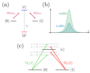
Figure 1: (a) Basic setup for the $\Lambda$-type system. The excited state decays to an additional low-lying level $|g\rangle$ with a rate $\gamma$. There is no coupling or decay with the computational subspace itself. This means that dissipation effects only occur while the excited state is populated. (b) Hyperbolic secant pulses as defined in Eq. (11). (c) Configuration and detunings in the two-qubit gate setup.

Let us now consider the qubit subspace $M(0)=\text{Span}\{|0\rangle,|1\rangle\}=\text{Span}\{|b\rangle,|d\rangle\}$ and its dynamics. The subspace evolves into $M(t)$, spanned by:

$$|\psi_{k}(t)\rangle=\exp\left(-i\int_{0}^{t}H_{I}^{\rm RWA}(t^{\prime})dt^{\prime}\right)|k\rangle=\mathcal{U}(t,0)|k\rangle,$$ (6)

where $\mathcal{U}(t,0)$ is the time-evolution operator in RWA and $k=0$ and $1$. In the bright-dark basis, the unitary matrix assumes the form Herterich2016

$$\mathcal{U}(t,0) = |d\rangle\langle d|+\cos\Phi(|b\rangle\langle b|+|e\rangle\langle e|)$$ (7)

$$-i\sin\Phi(|e\rangle\langle b|+|b\rangle\langle e|),$$

where

$$\Phi=\int_{0}^{t}\Omega(t^{\prime})dt^{\prime}$$ (8)

is the pulse area. Geometrically, this evolution corresponds to a path in the Grassmanian $\mathcal{G}(3;2)$, i.e., the set of two-dimensional subspaces of the three-dimensional Hilbert space that define the $\Lambda$-type system Bengtsson2006 . In particular, when we have $\Phi=\pi$, the trajectory corresponds to a full loop in the Grassmanian. The effect of this evolution whenever $\Phi=\pi$ is to implement a holonomy matrix

$$U(C)=\mathcal{U}(C)\mathbb{P}=\begin{matrix}\begin{pmatrix}\cos\theta&e^{-i\phi}\sin\theta\\ e^{i\phi}\sin\theta\ &-\cos\theta\end{pmatrix}\end{matrix}={\bf n}\cdot\bm{\sigma},$$ (9)

after properly projecting $\mathcal{U}(t,0)$ into the qubit space. Here, ${\bf n}=(\sin\theta\cos\phi,\sin\theta\sin\phi,\cos\theta)$ and $\mathbb{P}=|0\rangle\langle 0|+|1\rangle\langle 1|$. Besides, we have parametrized the frequencies $\omega_{0}$ and $\omega_{1}$ as $\omega_{0}=\sin(\theta/2)e^{i\phi}$ and $\omega_{1}=-\cos(\theta/2)$, i.e., $\theta$ and $\phi$ determine the relative amplitude and phase, respectively, of the two laser pulses. This process corresponds to a $\pi$ rotation around ${\bf n}$ on the Bloch sphere. The unitary in Eq. (9), however, is not universal (the phase-shift gate, for instance, cannot be written in this form). A universal gate can be implemented by employing a second loop $C_{{\bf m}}$, yielding

$$U(C)=U(C_{{\bf m}})U(C_{{\bf n}})={\bf n}\cdot{\bf m}-i\bm{\sigma}\cdot({\bf n}\times{\bf m}).$$ (10)

This transformation has a clear physical meaning as well; the universal gate $U(C)$ above corresponds to a rotation in the plane spanned by ${\bf n}$ and ${\bf m}$ by an angle of $2\cos^{-1}({\bf n}\cdot{\bf m})$ Sjoqvist2012 . Therefore, any single-qubit gate can be obtained by an appropriate choice of pulses, determined by ${\bf n}$ and ${\bf m}$. The holonomic nature of $U(C)$ in Eq. (10) relies on two facts Sjoqvist2012 : (i) the Hamiltonian matrix $\langle\psi_{k}(t)|H_{I}(t)|\psi_{l}(t)\rangle$ vanishes so that $U(C)$ becomes purely dependent on $C$, and (ii) there exist two generic loops $C$ and $C^{\prime}$ in $\mathcal{G}(3;2)$ for which the corresponding unitaries do not commute. The latter, together with the two-qubit setting described below, ensures universality of NHQC.

From hereafter, we use hyperbolic secant pulses

$$\Omega(t)=\beta\operatorname{sech}(\beta t),$$ (11)

as depicted in Fig. 1(b). The parameter $\beta$ can be regarded as the inverse pulse length: by increasing $\beta$ we implement sharper and shorter pulses. It also provides a convenient parametrization: this pulse is area-preserving and the condition $\Phi=\pi$ is satisfied regardless of the value of $\beta$ chosen.

Finally, we use the amplitude-damping jump operator $L=|g\rangle\langle e|$, with $|g\rangle$ being an additional low lying level, and the Lindblad equation

$$\frac{d\rho}{dt}=i[\rho,H_{I}(t)]+\gamma D(\rho),$$ (12)

to model decay Breuer2007 . Here, $\rho$ is the density matrix of the system, $D(\rho)=L\rho L^{\dagger}-\frac{1}{2}\{L^{\dagger}L,\rho\}$ is the dissipator, and $\gamma$ is the dissipation rate, as depicted in Fig. 1(a).

II.2 Two-qubit gate

The original NHQC proposal in Ref. Sjoqvist2012 includes a protocol based on the Sørensen–Mølmer scheme Sorensen1999 for implementing two-qubit gates (see also Ref. Duan2001 for an adiabatic implementation and Refs. ZhaoXu2019 ; Xu2021 for generalizations of the NHQC scheme to multi-qubit gates). The setup for the two-qubit gate consists of two identical trapped ions in the same three-level $\Lambda$-configuration as the one used for single-qubit gates. The transition $0\leftrightarrow e$ ($1\leftrightarrow e$) is driven by a laser with detuning $\pm(\nu+\delta)$ [$\pm(\nu-\delta)]$, where $\nu$ is the trap frequency and $\delta$ is an additional detuning, as shown in Fig. 1(c). In addition, we assume that the system satisfies the Lamb-Dicke criterion $\eta\ll 1$, where $\eta$ is the Lamb-Dicke parameter, and also that $|\Omega_{i}(t)|<\nu$. The parameter $\eta$ depends on the zero-point spread of the ion Wineland1998 and accounts for the coupling strength between its internal degrees of freedom and its motional states Li2002 . These conditions allow us to suppress the off-resonant couplings Sorensen1999 . As such, the Hamiltonian describing this interaction assumes the form

$$H^{(2)}(t) = \frac{\eta^{2}}{\delta}\bigg{(}|\Omega_{0}(t)|^{2}\sigma_{0}(\phi,t)\otimes\sigma_{0}(\phi,t)$$ (13)

$$-|\Omega_{1}(t)|^{2}\sigma_{1}(-\phi,t)\otimes\sigma_{1}(-\phi,t)\bigg{)},$$

where

$$\sigma_{0}(\phi,t)=e^{i\phi/4}(1+e^{-2if_{0e}t})|e\rangle\langle 0|+{\rm H.c.},$$

$$\sigma_{1}(-\phi,t)=e^{-i\phi/4}(1+e^{-2if_{1e}t})|e\rangle\langle 1|+{\rm H.c}.$$ (14)

After eliminating off-resonant couplings of the singly excited states $|0e\rangle$ , $|e0\rangle$, $|1e\rangle$ and $|e1\rangle$, and once again performing the RWA, the Hamiltonian reads:

$$H^{(2),{\rm RWA}}(t)=\sqrt{|\Omega_{0}(t)|^{4}+|\Omega_{1}(t)|^{4}}\left(\tilde{H}^{(2)}_{0}+\tilde{H}^{(2)}_{1}\right),$$ (15)

with

$$\tilde{H}^{(2)}_{0}=\sin{\frac{\theta}{2}}e^{i\phi/2}|ee\rangle\langle 00|-\cos{\frac{\theta}{2}}e^{-i\phi/2}|ee\rangle\langle 11|+{\rm H.c.}$$

and

$$\tilde{H}^{(2)}_{1}=\sin{\frac{\theta}{2}}|e0\rangle\langle 0e|-\cos{\frac{\theta}{2}}|e1\rangle\langle 1e|+{\rm H.c.}$$ (17)

Here, $|\Omega_{0}(t)|^{2}/|\Omega_{1}(t)|^{2}=\tan(\theta/2)$ and $\phi$ are kept constant throughout the pulse. Likewise, we should assume the criterion $\frac{\eta^{2}}{\delta}\int_{0}^{\tau}\sqrt{|\Omega_{0}(t)|^{4}+|\Omega_{1}(t)|^{4}}dt=\pi$ for the pulse area is satisfied. By analogy to the single-qubit gate, this procedure yields the unitary

$$U^{(2)}(C_{n}) = \cos{\theta}|00\rangle\langle 00|+e^{-i\phi}\sin{\theta}|00\rangle\langle 11|$$ (18)

$$+e^{i\phi}\sin{\theta}|11\rangle\langle 00|-\cos{\theta}|11\rangle\langle 11|$$

$$+|01\rangle\langle 10|+|10\rangle\langle 10|.$$

By choosing $\theta=0$, we are able to construct a controlled-$Z$ (CZ) gate

$$U^{(2)}_{\rm CZ}=|00\rangle\langle 00|+|01\rangle\langle 10|+|10\rangle\langle 10|-|11\rangle\langle 11|,$$ (19)

which is an entangling gate and can form a universal set together with a universal single-qubit gate Bremner2002 .

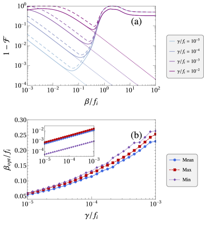
Figure 2: (a) The solid (dashed) lines correspond to the mean (maximum) infidelity $1-\mathcal{F}$ of the $S$ gate as a function of the ratio $\beta/f_{i}$ for different values of $\gamma/f_{i}$. The dotted lines correspond to the RWA solution where the Hamiltonian in Eq. (4) is used together with the master equation in Eq. (12), i.e., when counter-rotating effects are neglected. The spacing between the two pair of pulses is chosen as $\Delta t=10/\beta$. This guarantees that the pulses are not significantly overlapping. We used a grid of 500 sample points for $\beta/f_{i}$. (b) Optimal inverse pulse length $\beta_{opt}$ (in units of $f_{i}$) as a function of $\gamma/f_{i}$. We also plot the corresponding infidelity (inset). We have used a sample space of 1000 points for $\beta_{i}/f_{i}$ in the interval $[0.03,0.3]$. The average infidelity was calculated for $100$ input states uniformly sampled over the Bloch sphere in both figures.

III Results

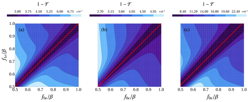
Figure 3: Average infidelity $1-\mathcal{F}$ as a function of the counter-rotating frequencies $f_{0e}$ and $f_{1e}$ for $\gamma/\beta=0.02$. Results are shown for (a) the $X$ gate, (b) the Hadamard gate, and (c) the $S$ gate. Other details and parameters are the same as those in Fig. 2. The simulations were done for a grid of $150\times 150$ frequencies $f_{0e}$ and $f_{1e}$.

The validity of the RWA has been studied previously in the dissipationless case for single-qubit gates Spiegelberg2013 . There, the authors show that the approximation starts to break down for very short pulses. We further extend this investigation, considering the competing effect of dissipation and counter-rotating terms; while faster gates avoid decoherent effects, we also observe the counter-rotating terms playing a larger role in the dynamics, compromising the fidelity of the gate. The converse is also true: if we use longer duration pulses in order to offset the counter-rotating terms, the accuracy suffers due to the longer exposure time to dissipative effects. Our objective is to find an optimal relationship between these parameters, namely, to investigate the interplay among three components in this model: the inverse pulse length $\beta$ defining the hyperbolic secant pulse in Eq. (11), the coupling parameter $\gamma$, and the counter-rotating frequencies $f_{je}$.

If we write Eq. (3) in terms of the bright and the dark states we obtain

$$H_{I}(t) = \Omega(t)(1+|\omega_{0}|^{2}e^{-2if_{0e}t}+|\omega_{1}|^{2}e^{-2if_{1e}t})|e\rangle\langle b|$$ (20)

$$\quad+\Omega(t)\omega_{0}\omega_{1}(e^{-2if_{1e}t}-e^{-2if_{0e}t})|e\rangle\langle d|+\mathrm{H.c.}$$

Differently from what we observe in the ideal case, the presence of counter-rotating terms introduces a coupling between the dark and the excited state. An exception occurs in the case of homogeneous frequencies, that is, when $f_{1e}=f_{0e}=f_{i}$, resulting in

$$H_{I}(t)=\Omega(t)(1+e^{-2if_{i}t})|e\rangle\langle b|+\mathrm{H.c.}$$ (21)

The equation above means that taking the two counter-rotating frequencies to be the same eliminates the coupling between the dark state and the excited state in Eq. (20). On the other hand, we can see that Eq. (21) differs from Eq. (5) by a factor of $e^{-2if_{i}t}$ in the Rabi frequency. This means that even though the structure of the Hamiltonian is the same as the one found in the ideal case, due to the counter-rotating corrections we do not, in general, return to the initial subspace at the end of the evolution.

III.1 Singe-qubit gates

In order to investigate the validity of the RWA, we compute the fidelity $\mathcal{F}=\langle\psi_{0}|U(C)^{\dagger}\rho U(C)|\psi_{0}\rangle$ for different quantum gates, and analyze the simulation results in terms of the infidelity $1-\mathcal{F}$. The unitary $U(C)$ corresponds to the ideal unitary in Eq. (10), which is determined by the choice of ${\bf n}$ and ${\bf m}$. The density matrix $\rho$ is obtained by solving the master equation, Eq. (12), for the non-RWA Hamiltonian in Eq. (3), and $|\psi_{0}\rangle$ is the input state. Finally, we compute the average fidelity for several input states uniformly distributed over the Bloch sphere. For details, see the Appendix.

We start by examining the average infidelity for the phase-shift gate. By choosing $\theta=\theta^{\prime}=\pi/2$ resulting in the pulses ${\bf n}=(\cos\phi,\sin\phi,0)$ and ${\bf m}=(\cos\phi^{\prime},\sin\phi^{\prime},0)$, we can implement the phase-shift gate $|k\rangle=e^{2ik(\phi^{\prime}-\phi)}|k\rangle$, with $k=0$ and $1$. Basic results are shown in Fig. 2(a) for the average infidelity $1-\mathcal{F}$ as a function of the ratio between the inverse pulse length $\beta$ and the counter-rotating frequencies taken to be the same, i.e., $f_{0e}=f_{1e}=f_{i}$. In Fig. 2(b), we also include the maximum and minimum infidelities in order to investigate how the gate might behave depending on the input state. They seem to play a minor role regarding the optimal configuration of the gate. While we observe a significant gap in the performance of the maximum and minimum achievable infidelities in the inset of Fig. 2(b), the infidelity as a function of $\beta/f_{i}$ behaves very similarly for different input states and the optimal inverse pulse length in Fig. 2(b) remains largely unchanged, specially at lower frequencies. Therefore, the mean infidelity is, by itself, able to capture the general behavior of the gates and its optimal configurations sufficiently well.

We can notice that for small $\beta/f_{i}$ (longer pulses) the curves should converge roughly to the same fidelity, but at different rates depending on $\gamma/f_{i}$. This is not visible in the plot for smaller rates of $\gamma/f_{i}$ due to the increasingly large timescales necessary to observe this effect, which make numerical simulations difficult. This happens due to the fact that in this regime the decoherent effects become dominant. More specifically, the dissipation hampers any population transfer between the qubit states, as in this case the populations and coherences in the excited state quickly decay to the ground state. Therefore, the final state is very nearly the same as the input state, regardless of the value of $\beta/f_{i}$. We make a quantitative support to this claim at the end of this section.

On the other hand, for large $\beta/f_{i}$ (shorter pulses) we can see that the gate accuracy also decreases and the fidelity becomes independent of the ratio $\gamma/f_{i}$. In this scenario the operation time is very short, hence the counter-rotating terms dominate and the end result depends on the particular value of $f_{i}$. The asymptotic behavior for $\gamma\ll f_{i}\ll\beta$ has been briefly discussed in Ref.Spiegelberg2013 for the $X$ and the Hadamard (${\rm H}$) gates, when considering a few selected input states. The counter-rotating correction in Eq. (21) becomes $1+e^{-2if_{i}t}\approx 2$ for small $f_{i}$. In this regime, the system undergoes a cyclic evolution twice. This means that the bright state evolves as $|b\rangle\rightarrow-|b\rangle\rightarrow|b\rangle$, and the net effect of the evolution is simply to (approximately) implement the identity gate, once again leaving the input state unchanged.

Finally, for values in-between we observe the optimal regime for the quantum gate and the presence of a global minimum in the infidelity $1-\mathcal{F}$. This is consistent with the intuitive idea behind the competition between the RWA and the dissipative effects: the optimal pulse duration should be long enough in order to minimize the counter-rotating contributions to the dynamics while also being short enough to avoid dissipative losses. After that point the RWA starts to break down and the infidelity increases. Figure 2 (a) explicitly shows an overlap between the RWA solution (dashed line) and the full solution (solid lines). The latter deviates from the former when $\beta/f_{i}$ approaches the global minimum, explicitly showing a breakdown of the RWA. Therefore, for optimal performance, the frequencies and the pulse should be tuned in a way that $f_{i}>\beta\gg\gamma$ holds, if possible. This means that the inverse pulse length $\beta$ should be much larger than $\gamma$, and at the same time the counter-rotating frequencies should be sufficiently larger than $\beta$.

III.2 Heterogeneous frequencies

We also examine how different counter-rotating frequencies affect the fidelity of the gates. In Fig. 3 we show a contour plot for the infidelity $1-\mathcal{F}$ as a function of $f_{je}/\beta$ for three different gates. Results are shown for the $X$, ${\rm H}$, and $S$ gates, respectively. The red lines correspond to the optimal frequency $f_{1e}$ for a given $f_{0e}$. A few observations can be made from these plots. Foremost, we can explicitly see that for the range of frequencies considered here the $S$ gate has a worse fidelity in general. This corroborates the fact that, since the $S$ gate requires two pulses, the longer operation time makes the gate much more susceptible to open quantum system effects. Additionally, it is also possible to observe that Fig. 3(a) is symmetric, while Fig. 3(b) is not. This is linked to the fact that the complex frequencies $\omega_{0}$ and $\omega_{1}$ are of the same modulus for the $X$ gate, but not for the Hadamard gate.

Furthermore, we can analyze the optimal combinations of frequencies in Fig. 3. The results shown in Figs. 3(a) and  3(b) show that for single pulse gates and for the frequency range considered, the optimal relationship for the counter-rotating frequencies is to take both of them to be the same, i.e., the infidelity $1-\mathcal{F}$ is minimum for $f_{0e}=f_{1e}$. This is possibly a result of the decoupling of the dark and the excited states, which happens in Eqs. (20) and (21). The coupling between $|e\rangle$ and $|d\rangle$ in Eq. (20) seems to play a larger role than the presence of the counter-rotating correction in Eq. (21). Increasing one of the frequencies while keeping the other to be the same shows no noticeable improvement. On the contrary, we observe a slight worsening of the gate performance.

Surprisingly, we observe a different behavior for the $S$ gate: there is a slight offset between the optimal $f_{0e}$ and $f_{1e}$. The result indicates that ideally one should increase these two frequencies at a constant ratio, different from unity. This behavior may arise from the use of two pair of pulses in the $S$ gate implementation. It has been verified in Ref. Spiegelberg2013 that the fidelity of non-commuting gates is actually lower than the product of their fidelities. A similar mechanism may be playing a role here: the non-Abelian behavior of the unitaries in Eq. (10) is possibly the reason why we observe this effect for unequal frequencies in the S gate.

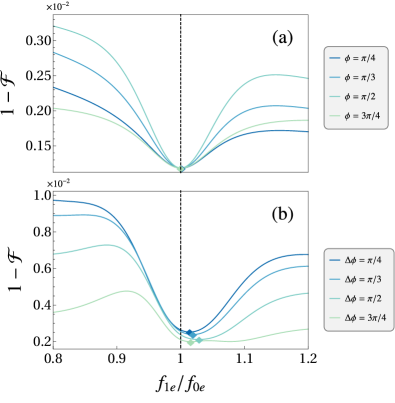
Figure 4: Infidelity as a function of the ratio $f_{1e}/f_{0e}$ for single-qubit gates. We show the results for (a) a single-pulse gate with $\theta=\pi/4$, for different values of $\phi$. In panel (b) we plot the results for the phase-shift gate, for which $\theta=\theta^{\prime}=\pi/2$, for different values of $\Delta\phi\equiv\phi^{\prime}-\phi$. We observe a slight shift in the optimal ratio for the phase-shift gates. The optimal points depends on the desired phase. Here, the coupling strength is given by $\gamma/\beta=10^{-3}$, the spacing between the pulses is $\Delta t=20/\beta$ and the frequency $f_{0e}$ is fixed and given by $f_{0e}/\beta=10$. We use a sampling space of $250$ frequencies and $100$ input states, as described in Fig. 2.

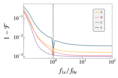
Figure 5: Infidelity as a function of the ratio $f_{1e}/f_{0e}$ for the NOT gate (yellow), the Hadamard gate (magenta), the $Z$ gate (purple) and the $S$ gate (dark blue). The decay rate, the sampling space and $f_{e0}$ are the same as those in Fig. 4. Note that the minimum for the $S$ gate is slightly displaced from $f_{1e}/f_{0e}=1$ (dashed line), in accordance with Figs. 3(c) and 4.

Now, we further investigate the effect of heterogeneous frequencies. For that we consider the infidelity of two different single qubit gates. For the first gate we implement the single-pulse gate in Eq. (9) for different values of $\phi$, with $\theta=\pi/4$. For the second gate, we implement the phase-shift gate for different phases $\Delta\phi=2(\phi^{\prime}-\phi)$. Our objective is to analyze how changing $\phi$ affects the optimal ratio between the two counter-rotating frequencies. Like Fig. 3, the curves in Fig. 4(a) show that single-pulse gates achieve optimality for equal frequencies. On the other hand, Fig. 4(b) shows that while the optimal ratio indeed occurs for different frequencies, the gain is very marginal. This suggests that a weak coupling between the excited state and the dark state alone is much more relevant overall. This claim is further supported by the result in Fig. 5.

We see, for the $X$, ${\rm H}$ and $S$ gates, that there is a sudden decrease in the infidelity when $f_{0e}\approx f_{1e}$. For the $S$ and the $X$ gates the point $f_{0e}=f_{1e}$ is actually a global minimum. Meanwhile, when the ${\rm H}$ gate is considered, the point where the two frequencies are the same only happens to be a local minimum. For the ${\rm Z}$ gate we observe no minimum at all, and the infidelity is simply monotonically decreasing with $f_{1e}/f_{0e}$. Hence, whether the point $f_{0e}=f_{1e}$ is optimal may depend on the particular gate implementation and on the frequency range considered. Nevertheless, a characteristic drop in the infidelity around this region seems to be common among all of the gates but the $Z$ gate, and the performance in the regime where $f_{0e}=f_{1e}$ is quite similar to the one obtained when $f_{1e}\gg f_{0e}$. The behavior of the curves in Fig. 5 arises mainly because of the last term in Eq. (20). For the ${\rm Z}$ gate, for instance, we have $\omega_{0}=0$ and $\omega_{1}=1$. In this very particular case, this term vanishes and the fidelity actually depends only on $f_{1e}$, and we do not observe any coupling between the dark state and the excited state regardless of $f_{0e}$. Meanwhile, the $X$ gate is quite different: since $|\omega_{0}|=|\omega_{1}|=1/\sqrt{2}$, the dependence of the infidelity on $f_{0e}$ and $f_{1e}$ is symmetric and the product $\omega_{0}\omega_{1}$ is maximum (in modulus), thus, the $X$ gate (or any other gate for which $|\omega_{0}|=|\omega_{1}|$, for that matter) is the most sensitive to the coupling between the dark state and the excited state. For other gates, such as the Hadamard gate, we observe a behavior in-between. The ratio $|\omega_{1}|/|\omega_{0}|$ between the amplitudes should then play some role whether the optimal strategy is to take $f_{1e}/f_{0e}=1$ or $f_{1e}\gg f_{0e}$ for maximum fidelity.

III.3 Two-qubit gates

Finally, we check the robustness against both effects in the case of the two-qubit gate. Considering the counter-rotating contributions in Eqs. (13) and (II.2), Eqs. (II.2) and (17) become

$$H^{(2)}_{0}(t) = (1+e^{-2if_{0e}t})^{2}\sin{\frac{\theta}{2}}e^{i\phi/2}|ee\rangle\langle 00|$$ (22)

$$-(1+e^{-2if_{1e}t})^{2}\cos{\frac{\theta}{2}}e^{-i\phi/2}|ee\rangle\langle 11|+{\rm H.c.}$$

and

$$H^{(2)}_{1}(t) = 4\cos^{2}{(f_{0e}t)}\sin{\frac{\theta}{2}}|e0\rangle\langle 0e|$$ (23)

$$-4\cos^{2}{(f_{1e}t)}\cos{\frac{\theta}{2}}|e1\rangle\langle 1e|+{\rm H.c.},$$

respectively. We perform simulations for the CZ gate, which can be constructed by taking $\theta=0$. Results for the infidelity are shown in Fig. 6 as a function of the inverse pulse length $\beta$ (in units of $f_{1e}=f_{0e}=f_{i}$). We plot the infidelity, averaged over four different input states: $|+\rangle|+\rangle$, $|+\rangle|-\rangle$, $|-\rangle|+\rangle$ and $|-\rangle|-\rangle$ with $|\pm\rangle=(|0\rangle\pm|1\rangle)/\sqrt{2}$, which are states of interest since the application of the CZ gate upon them results in maximally entangled Bell states. Our results are qualitatively similar to what was obtained for the single-qubit case, showing that the two-qubit gate is also robust against the joint effect of dissipation and counter-rotating terms. Moreover, the asymptotic behavior for larger pulses is even more evident in Fig. 6; we can clearly see how the dissipative effects quickly start to dominate for $\beta/f_{i}\lesssim 4\cdot 10^{-3}$, eventually converging to a specific value, in a similar fashion to what we obtained for the phase-shift gate. The same phenomenon occurs when $\beta\gtrsim f_{i}$ due to the increasing influence of counter-rotating contributions. This behavior arises precisely due to the two mechanisms we have discussed before: for both the very fast or the very slow gate operation regimes, a given input state $|\psi_{0}\rangle$ is left roughly unchanged after the evolution, and the fidelity associated with the process is approximately $|\langle\psi_{0}|U(C)|\psi_{0}\rangle|^{2}$. One may then find the asymptotic value for the average infidelity $1-\mathcal{F}$ in Figs. 2 and 6 by averaging $|\langle\psi_{0}|U(C)|\psi_{0}\rangle|^{2}$ over all the input states. It is possible to show that $1-\mathcal{F}=1/3$ for the phase-shift gate in either cases. This is not visible in Fig. 2 (a) simply due to the fact that we would need to use pulses of the order of $\beta/f_{i}\approx 10^{-4}$ or smaller in order to observe such a strongly dissipative regime. Moreover, by comparing Figs. 2 and 6 we could think that single and two-qubit gates are similarly robust, but that is not necessarily the case. As we can see in Figs. 3(a) and 3(b) and also in Fig. 5, single-pulse gates typically have lower infidelities. On the other hand, a positive feature is that the optimal pulse-length seems quite similar for both single- and two-qubit gates, which might simplify experimental realizations of holonomic quantum gates.

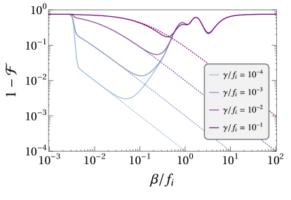
Figure 6: Infidelity of the CZ gate as a function of $\beta/f_{i}$. Dotted lines represent the RWA solution given by the Hamiltonian in Eq. (II.2). Other details are the same as those in Fig. 2.

III.4 Experimental feasibility

On a closing note, we briefly discuss the experimental feasibility of an investigation regarding the frequency asymmetry. In Ref. AbdumalikovJr2013 , for instance, the experiment is performed for a ratio of $f_{0e}/f_{1e}\approx 1.04$ between the frequencies and a dissipation rate given by $\gamma/f_{i}\approx 1.1\cdot 10^{-4}$. As we can see in Fig. 4, these parameters are close to the optimal scenario for both single and two-pulse gates. However, fine-tuning the frequencies to be the same in this setup in order to achieve even lower infidelities could be somewhat challenging. This implementation uses a transmon qubit based on a nearly harmonic ladder, where its ground state and second excited state span the qubit subspace and the first excited state plays the role of the auxiliary state $|e\rangle$. The anharmonicity is used to average out an undesirable coupling between the $\Lambda$-type system subspace and higher energy levels. Thus, homogeneous frequencies could possibly give rise to unwanted dynamical contributions. In this sense, implementations based on ion traps could be used to fine-tune the bare energy levels as desired, reaching the configuration shown in Figs. 4 and 5 for the gates where homogeneous frequencies are optimal.

IV Conclusions

We have investigated the robustness of non-adiabatic holomonic quantum gates against dissipative effects and counter-rotating dynamical contributions due to the energy structure of the $\Lambda$-type system. While short run times minimize the dissipative losses, the counter-rotating frequencies induce oscillations, which compromise the geometric character of the gate, decreasing its overall fidelity. In a real implementation, one should seek to sufficiently approach the RWA regime while keeping losses due to open quantum system effects minimal. In this work we have explored this trade-off in detail, obtaining an optimal regime of operation for single and two-qubit gates for a range of parameters typically found in experimental scenarios. Thus, we believe that our analysis could provide a suitable rule-of-thumb for optimal experimental parameters, as well as open up for optimization of gate performance by varying the pulse length, in implementations of quantum gates in the $\Lambda$-setting.

Moreover, we have also studied how different frequencies affect the performance of single-qubit gates. We showed that counter-rotating corrections introduce an unwanted coupling between the dark state and the excited state in the $\Lambda$-type system. Homogeneous frequencies in general result in a sudden decrease of the infidelity due to the suppression of the dark state coupling. However, whether this regime is indeed optimal will depend on the gate which is being implemented. In addition, we have observed that two-pulse single-qubit gates might display an optimal configuration for slightly heterogeneous frequencies. We suspect that this behavior arises due to the non-Abelian property of the geometrical phases. This phenomenon can also be observed for square pulses in a slightly different fashion. However, whether our results still hold for arbitrary pulses shapes remain an open question and is subject for further investigation.

Future directions of study could either probe into generalizations of this analysis to different implementations of the holonomic protocol, such as the off-resonant scheme Xu2015 ; Sjoqvist2016 , the single loop scheme Herterich2016 , time-optimal-control Chen2020 ; Han2020 and path shortening Xu2018b schemes, and environment assisted implementations Ramberg2019 , or into inclusions of other open system effects, such as dephasing and correlated two-qubit noise. A generalization to multi-qubit gates ZhaoXu2019 ; Xu2021 or strategies which do not rely on the RWA Gontijo2020 could also be investigated.

Appendix A APPENDIX: UNIFORM SAMPLING OVER THE BLOCH SPHERE

Here, we show how the Fibonacci nodes algorithm Hardin2016 can be implemented. The algorithm can be used to uniformly sample states over the Bloch sphere. Canonical approaches for this problem based on, e.g., random sampling Muller1959 can also be used. However, the method presented here is deterministic, making it possible to get a reasonable approximation even for a smaller number of points. This greatly reduces the time required for computing the average fidelity, since we can perform simulations for a smaller number of input states. To implement the algorithm one should follow the steps below:

1. Uniformly distribute the $z$-coordinate $z_{n}$ of the points in the interval $[1,-1]$.

2. Distribute the azimuthal angles as $\phi_{n}=2\pi\phi n$, where $\phi=(1+\sqrt{5})/2$ is the golden ratio.

3. Take $x_{n}=\sqrt{1-z_{n}^{2}}\cos{\phi_{n}}$ and $y_{n}=\sqrt{1-z_{n}^{2}}\sin{\phi_{n}}$.

4. The points are given by the set of triples $(x_{n},y_{n},z_{n})$, for $n=1,...,N$.

This set of triples can then be used to distribute the input states over the Bloch sphere.

References

- (1) D. P. DiVincenzo, The physical implementation of quantum computation, Fortschritte der Phys. 48, 771 (2000).
- (2) E. Joos and H. D. Zeh, The emergence of classical properties through interaction with the environment, Z. Phys. B 59, 223 (1985).
- (3) W. G. Unruh, Maintaining coherence in quantum computers, Phys. Rev. A 51, 992 (1995).
- (4) A. Barenco, C. H. Bennett, R. Cleve, D. P. DiVincenzo, N. Margolus, P. Shor, T. Sleator, J. A. Smolin, and H. Weinfurter, Elementary gates for quantum computation, Phys. Rev. A 52, 3457 (1995).
- (5) P. Zanardi and M. Rasetti, Holonomic quantum computation, Phys. Lett. A 264, 94 (1999).
- (6) J. Pachos, P. Zanardi, and M. Rasetti, Non-Abelian Berry connections for quantum computation, Phys. Rev. A 61, 010305(R) (1999).
- (7) L.-M. Duan, J. I. Cirac, and P. Zoller, Geometric Manipulation of Trapped Ions for Quantum Computation, Science 292, 1695 (2001).
- (8) P. Solinas, M. Sassetti, P. Truini, and N. Zanghì , On the stability of quantum holonomic gates, New J. Phys. 14, 093006 (2012).
- (9) L. Viotti, F. C. Lombardo, and P. I. Villar, Geometric phase in a dissipative Jaynes-Cummings model: Theoretical explanation for resonance robustness, Phys. Rev. A 105, 022218 (2022).
- (10) M. V. Berry, Quantal phase factors accompanying adiabatic changes, Proc. R. Soc. London, Ser. A 392, 45 (1984).
- (11) J. Anandan, Non-adiabatic non-Abelian geometric phase, Phys. Lett. A 133, 171 (1988).
- (12) E. Sjöqvist, D. M. Tong, L. M. Andersson, B. Hessmo, M. Johansson, and K. Singh, Non-adiabatic holonomic quantum computation, New J. Phys. 14, 103035 (2012).
- (13) X.-B. Wang and M. Keiji, Nonadiabatic Conditional Geometric Phase Shift with NMR Phys. Rev. Lett. 87, 097901 (2001).
- (14) Shi-Liang Zhu and Z. D. Wang, Implementation of Universal Quantum Gates Based on Nonadiabatic Geometric Phases, Phys. Rev. Lett. 89, 097902 (2002).
- (15) M. Johansson, E. Sjöqvist, L. M. Andersson, M. Ericsson, B. Hessmo, K. Singh, and D. M. Tong, Robustness of nonadiabatic holonomic gates, Phys. Rev. A 86, 062322 (2012).
- (16) P. Shen, T. Chen, and Z.-Y. Xue, Ultrafast Holonomic Quantum Gates, Phys. Rev. Appl. 16, 044004 (2021).
- (17) A. A. Abdumalikov Jr, J. M. Fink, K. Juliusson, M. Pechal, S. Berger, A. Wallraff, and S. Filipp, Experimental realization of non-Abelian non-adiabatic geometric gates, Nature (London) 496, 482 (2013).
- (18) S. Danilin, A. Vepsäläinen, and G. S. Paraoanu, Experimental state control by fast non- Abelian holonomic gates with a superconducting qutrit, Phys. Scr. 93, 055101 (2018).
- (19) S. Arroyo-Camejo, A. Lazariev, S. W. Hell, and G. Balasubramanian, Room temperature high-fidelity holonomic single-qubit gate on a solid-state spin, Nat. Commun. 5, 4870 (2014).
- (20) C. Zu, W.-B. Wang, L. He, W.-G. Zhang, C.-Y. Dai, F. Wang, and L.-M. Duan, Experimental realization of universal geometric quantum gates with solid-state spins, Nature (London) 514, 72 (2014).
- (21) G. F. Xu, C. L. Liu, P. Z. Zhao, and D. M. Tong, Nonadiabatic holonomic gates realized by a single-shot implementation, Phys. Rev. A 92, 052302 (2015).
- (22) E. Sjöqvist, Nonadiabatic holonomic single-qubit gates in off-resonant systems, Phys. Lett. A 380, 65 (2016).
- (23) E. Herterich and E. Sjöqvist, Single-loop multiple-pulse nonadiabatic holonomic quantum gates, Phys. Rev. A 94, 052310 (2016).
- (24) B. B. Zhou, P. C. Jerger, V. O. Shkolnikov, F. J. Heremans, G. Burkard, and D. D. Awschalom, Holonomic Quantum Control by Coherent Optical Excitation in Diamond, Phys. Rev. Lett. 119, 140503 (2017).
- (25) Y. Xu, W. Cai, Y. Ma, X. Mu, L. Hu, T. Chen, H. Wang, Y. P. Song, Z.-Y.nXue, Z.-q. Yin, and L. Sun, Single-Loop Realization of Arbitrary Nonadiabatic Holonomic Single-Qubit Quantum Gates in a Superconducting Circuit, Phys. Rev. Lett. 121, 110501 (2018).
- (26) G. F. Xu, D. M. Tong, and E. Sjöqvist, Path-shortening realizations of nonadiabatic holonomic gates, Phys. Rev. A 98, 052315 (2018).
- (27) T. Chen, P. Shen, and Z.-Y. Xue, Robust and Fast Holonomic Quantum Gates with Encoding on Superconducting Circuits, Phys. Rev. Appl. 14, 034038 (2020).
- (28) Z. Han, Y. Dong, B. Liu, X. Yang, S. Song, L. Qiu, D. Li, J. Chu, W. Zheng, J. Xu, T. Huang, Z. Wang, X. Yu, X. Tan, D. Lan, M.-H. Yung, and Y. Yu, Experimental realization of universal time-optimal non-abelian geometric gates, arXiv:2004.10364.
- (29) J. Spiegelberg and E. Sjöqvist, Validity of the rotating-wave approximation in nonadiabatic holonomic quantum computation, Phys. Rev. A 88, 054301 (2013).
- (30) G. Florio, P. Facchi, R. Fazio, V. Giovannetti, and S. Pascazio, Robust gates for holonomic quantum computation, Phys. Rev. A 73, 022327 (2006).
- (31) G. Florio, Decoherence in holonomic quantum computation, Open Syst. Inf. Dyn. 13, 263 (2006).
- (32) C. Lupo, P. Aniello, M. Napolitano, and G. Florio, Robustness against parametric noise of nonideal holonomic gates, Phys. Rev. A 76, 012309 (2007).
- (33) I. Bengtsson and K. Zyczkowski, Geometry of Quantum States (Cambridge University Press, Cambridge, England, 2006).
- (34) H.-P. Breuer and F. Petruccione, The Theory of Open Quantum Systems (Oxford University Press, Oxford, 2007).
- (35) A. Sørensen and K. Mølmer, Quantum Computation with Ions in Thermal Motion, Phys. Rev. Lett. 82, 1971 (1999).
- (36) P. Z. Zhao, G. F. Xu, and D. M. Tong, Nonadiabatic holonomic multiqubit controlled gates, Phys. Rev. A 99, 052309 (2019).
- (37) G. F. Xu, P. Z. Zhao, E. Sjöqvist, and D. M. Tong, Realizing nonadiabatic holonomic quantum computation beyond the three-level setting, Phys. Rev. A 103, 052605 (2021).
- (38) D. J. Wineland, C. Monroe, W. M. Itano, D. Leibfried, B. E. King, and D. M. Meekhof, Experimental Issues in Coherent Quantum-State Manipulation of Trapped Atomic Ions, J. Res. Natl. Inst. Stand. Technol. 103, 259 (1998).
- (39) X.-Q. Li, L.-X. Cen, G. Huang, L. Ma, and Y. Yan, Nonadiabatic Geometric Quantum Computation with Trapped Ions, Phys. Rev. A 66, 042320 (2002).
- (40) M. J. Bremner, C. M. Dawson, J. L. Dodd, A. Gilchrist, A. W. Harrow, D. Mortimer, M. A. Nielsen, and T. J. Osborne, Practical Scheme for Quantum Computation with Any Two-Qubit Entangling Gate, Phys. Rev. Lett. 89, 247902 (2002).
- (41) N. Ramberg and E. Sjöqvist, Environment-Assisted Holonomic Quantum Maps, Phys. Rev. Lett. 122, 140501 (2019).
- (42) M. M. Gontijo and J. C. A. Barata, Phase Factors of Periodically Driven Two-Level Systems, Phys. Scr. 95, 055101 (2020).
- (43) D. P. Hardin, T. Michaels, and E. B. Saff, A Comparison of Popular Point Configurations on , Dolomites Res. Notes on Approximation 9, 16 (2016).
- (44) M. E. Muller, A note on a method for generating points uniformly on -dimensional spheres, Commun. ACM 2, 19 (1959).