reXcor: A Model of the X-ray Spectrum of Active Galactic Nuclei that Combines Ionized Reflection and a Warm Corona

Abstract

The X-ray spectra of active galactic nuclei (AGNs) often exhibit an excess of emission above the primary power-law at energies $\la 2$ keV. Two models for the origin of this ‘soft excess’ are ionized relativistic reflection from the inner accretion disc and Comptonization of thermal emission in a warm corona. Here, we introduce reXcor, a new AGN X-ray ($0.3$–$100$ keV) spectral fitting model that self-consistently combines the effects of both ionized relativistic reflection and the emission from a warm corona. In this model, the accretion energy liberated in the inner disc is distributed between a warm corona, a lamppost X-ray source, and the accretion disc. The emission and ionized reflection spectrum from the inner $400$ $r_{g}$ of the disc is computed, incorporating the effects of relativistic light-bending and blurring. The resulting spectra predict a variety of soft excess shapes and sizes that depend on the fraction of energy dissipated in the warm corona and lamppost. We illustrate the use of reXcor by fitting to the joint XMM-Newton and NuSTAR observations of the Seyfert 1 galaxies HE 1143-1820 and NGC 4593, and find that both objects require a warm corona contribution to the soft excess. Eight reXcor table models, covering different values of accretion rate, lamppost height and black hole spin, are publicly available through the XSPEC website. Systematic use of reXcor will provide insight into the distribution of energy in AGN accretion flows.

1 Introduction

At energies $\la 2$ keV the X-ray spectra of most active galactic nuclei (AGNs) exhibit an excess of emission above what is expected from the primary hard X-ray power-law (e.g., Piconcelli et al., 2005; Scott et al., 2012; Winter et al., 2012; Ricci et al., 2017; Gliozzi & Williams, 2020). This ‘soft excess’ can be modeled as a thermal emitter (e.g., Turner & Pounds, 1989; Bianchi et al., 2009), but the resulting temperatures do not appear to vary with the black hole mass or accretion rates, in contrast with expectations from standard accretion disc theories (e.g., Gierliński & Done, 2004; Bianchi et al., 2009). Therefore, the origin of the soft excess is expected to be closely related to local atomic and radiative processes within the accretion disc (e.g., Gierliński & Done, 2004; Crummy et al., 2006). The detection of high frequency soft lags from numerous bright Seyferts shows that some fraction of the soft excess originates at a distance of a few gravitational radii ($r_{g}=GM/c^{2}$, where $M$ is the black hole mass) from the hard X-ray emitting corona (e.g., De Marco et al., 2013; Kara et al., 2016; Cackett et al., 2021).

While these reverberation measurements show that at least some part of the soft excess is produced by the reprocessing of irradiating X-rays (a process known as X-ray reflection; Fabian & Ross 2010), other processes occurring within the accretion disc are likely to contribute to the soft excess (e.g., Keek & Ballantyne, 2016). Evidence for this additional component can be seen from the difficulties faced by reflection models when fitting broadband X-ray spectra of AGNs (e.g., Matt et al., 2014; Porquet et al., 2018; Laha & Ghosh, 2021; Xu et al., 2021a). Although the models provide an adequate description of the data, the strength of the soft excess can drive the models to extreme conditions, such as high disc densities, large iron abundances, or small inclination angles (e.g., Crummy et al., 2006; García et al., 2019; Jiang et al., 2019a, 2020; Middei et al., 2020). Therefore, there has been significant interest in determining other sources for the soft excess that can alleviate the challenges faced by a reflection origin.

In recent years, interest has focused on the idea of a ‘warm corona’ as an alternative origin for the soft excess. A warm corona is a Comptonizing layer at the surface of the accretion disc with a Thomson depth of $\tau\sim 10$–$40$ and temperature $kT\sim 0.1$–$1$ keV (e.g., Magdziarz et al., 1998; Matt et al., 2014; Kubota & Done, 2018; Petrucci et al., 2018). This layer, heated by internal dissipation of accretion energy, would produce the soft excess by scattering the thermal emission from the bulk of the disc as it passes through the warm corona (e.g., Mehdipour et al., 2015). Although a straightforward warm Comptonization model provides a good fit to the observed soft excess in many AGNs (e.g., Petrucci et al., 2018; Middei et al., 2018, 2019, 2020; Ursini et al., 2020), there are concerns about the physical plausibility of the scenario. For example, García et al. (2019) argued that thermal disc emission passing through a $\sim 1$ keV gas should be imprinted with many soft X-ray absorption lines, which are not observed in AGN spectra. On the theoretical side, Różańska et al. (2015) and Gronkiewicz & Różańska (2020) showed that significant magnetic pressure support is required to produce a $\tau\sim 10$ warm corona in hydrostatic equilibrium.

Recently, Ballantyne (2020) found that the hard X-ray power-law illuminating the surface of a warm corona is crucial to both heating the layer and providing a base level of ionization in the gas. As a result of the X-ray heating and ionization, thermal radiation passing through the warm corona would avoid being lost to soft X-ray absorption lines. Ballantyne (2020) also showed that a warm corona can produce a smooth soft excess, but only for a limited range of gas densities and temperatures. The implications of these results is that any warm corona must be placed close to the hard X-ray emission region in order to have sufficient ionization, and that changes in the soft excess may closely track structural changes in the warm corona (Ballantyne & Xiang, 2020). Similar conclusions on the warm corona properties under the conditions of X-ray illumination were found independently by Petrucci et al. (2020).

The picture that emerges from these studies is that while relativistic reflection and a warm corona are both plausible origins for the soft excess, the combination of the two scenarios may be a natural output from the inner accretion disc of AGNs (e.g., Porquet et al., 2018; Porquet et al., 2021; Xu et al., 2021b). In order to explore this idea further, we describe and present in this paper results from reXcor, a new publicly available, phenomenological AGN X-ray fitting model that self-consistently includes emission from both a warm corona and relativistically blurred ionized reflection. Application of reXcor to X-ray spectral data will show how these two components combine to produce the soft excess, and lead to constraints on how the accretion energy flows between the hot and warm coronae in AGN discs.

We describe the ingredients of reXcor and how it is calculated in the next section. An overview of the resulting spectral model and how the spectra change in response to the model parameters is provided in Sect. 3. We illustrate the use of reXcor in Sect. 4 where the model is used to fit a series of XMM-Newton and NuSTAR spectra from two AGNs, HE 1143-1820 and NGC 4593. Finally, a summary of the paper is presented in Sect. 5. Table models of reXcor spectra are available for use by the community at the XSPEC website.

2 Model Description

A reXcor model is constructed by integrating the reflection and emission spectrum produced by an AGN accretion disc from an inner radius ($r_{\mathrm{in}}=r_{\mathrm{ISCO}}+0.5$, where $r_{\mathrm{ISCO}}$ is the radius of the innermost stable circular orbit of a prograde accretion disc and all distances are in units of $r_{g}$) to an outer radius, $r_{\mathrm{out}}=400$. Below, we first describe how the spectrum is computed at a specific disc radius $r$, and then explain the integration procedure to construct the final spectrum. A schematic diagram of our model set-up, with references to the equations described below, is shown in Figure 1.

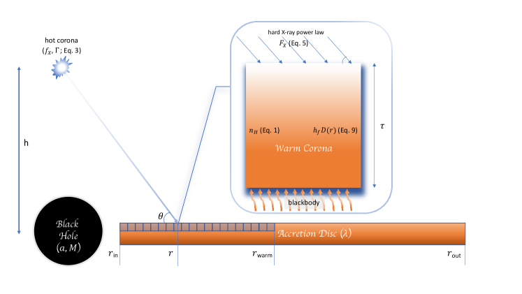
Figure 1: A schematic illustration of the ingredients behind the calculation of a reXcor spectrum. A hot corona in a lamppost geometry is situated at a height $h$ above a black hole of mass $M$ and spin $a$. The lamppost produces a power-law spectrum (with photon-index $\Gamma$) with a luminosity parameterized by $f_{X}$ (Eq. 3). The hard X-ray power-law illuminates the surface of a thin accretion disc with accretion rate $\lambda$. The flux at the disc surface is given by Eq. 5 which incorporates the effects of lightbending. We consider a column of irradiated gas with Thomson depth $\tau$ and constant density $n_{\mathrm{H}}$ (Eq. 1). This column is also heated by a warm corona which dissipates an energy flux $h_{f}D(r)$ (Eq. 9) in the gas. In addition to the internal heating and external X-ray illumination, thermal blackbody radiation from the bulk of the disc may enter the slab from below. We compute the X-ray reflection and emission spectrum from this slab at radius $r$, and integrate these spectra over the disc to produce the final reXcor model, including the effects of relatvistic blurring (see Sects. 2.1 and 2.2 for complete details).

2.1 The Reflection and Emission Spectrum at Radius $r$

The calculation of the X-ray spectrum from a disc radius $r$ that includes the effects of both reflection and a warm corona largely follows the procedure described by Ballantyne (2020) and Ballantyne & Xiang (2020). We compute the reflection and emission spectrum from a one-dimensional slab located at the surface of an accretion disc with hydrogen number density $n_{\mathrm{H}}$ and Thomson depth $\tau$. To determine the density of the slab, the mid-plane density is computed following the Svensson & Zdziarski (1994) radiation-pressure dominated disc solution and then divided by $10^{3}$ to mimic the fall-off in density from the mid-plane to the surface (e.g., Jiang et al., 2019b). Assuming $n_{\mathrm{H}}=\rho/m_{\mathrm{p}}$, where $\rho$ is the gas density and $m_{\mathrm{p}}$ is the mass of a proton, the hydrogen number density in the slab is

$$n_{\mathrm{H}}=(2.4\times 10^{15})\left(\frac{\eta}{0.1}\right)^{2}\left(\frac{\alpha}{0.1}\right)^{-1}\left(\frac{M}{\mathrm{M}_{\odot}}\right)^{-1}\lambda^{-2}r^{3/2}J(r)^{-2}\ \mathrm{cm^{-3}},$$ (1)

where $\eta$ is the radiative efficiency of the accretion process, $\alpha$ is the Shakura & Sunyaev (1973) viscosity parameter, and $J(r)=1-(r_{\mathrm{ISCO}}/r)^{1/2}$. In addition, the Eddington ratio of the AGN is $\lambda=L_{\mathrm{bol}}/L_{\mathrm{Edd}}$, where $L_{\mathrm{bol}}$ is the bolometric luminosity and $L_{\mathrm{Edd}}=4\pi GMm_{\mathrm{p}}c/\sigma_{\mathrm{T}}$ is the Eddington luminosity. Throughout this paper, both $\alpha$ and $\eta$ are fixed at $0.1$. For simplicity, we remove the dependence on the black hole spin in Eq. 1 by assigning $r_{\mathrm{ISCO}}=1.45$ when calculating $n_{\mathrm{H}}$. As a result, for a given black hole mass the disc density depends only on $\lambda$ and $r$.

The slab of gas at $r$ is illuminated from above by a stationary X-ray emitting hot corona that is located at a height $h$ (in units of $r_{g}$) above the rotational axis of the black hole (i.e., a lamppost geometry; e.g., Matt et al. 1991; Martocchia & Matt 1996; Dauser et al. 2013). This geometry is consistent with recent reverberation results indicating that the corona must be compact and located close to the central black hole (De Marco et al., 2013; Kara et al., 2016). The hot corona emits a power-law spectrum with photon index $\Gamma$ (i.e., the photon flux $\propto E^{-\Gamma}$) and exponential cutoff energies at both $30$ eV and $300$ keV to account for its Comptonization origin (e.g., Petrucci et al., 2001). The highest energy considered by the Ballantyne et al. (2001) code is 98 keV, so the precise value of the high-energy roll-over has minimal effect on the results.

Each side of the disc produces an energy flux $D(r)$ due to dissipation within the disc (Shakura & Sunyaev, 1973) where

$$D(r)=(6.89\times 10^{27})\left(\frac{\eta}{0.1}\right)^{-1}\left(\frac{M}{\mathrm{M}_{\odot}}\right)^{-1}\lambda r^{-3}J(r)\ \mathrm{erg\ cm^{-2}\ s^{-1}.}$$ (2)

The total X-ray luminosity of the hot corona is related to a constant fraction $f_{X}$ of $D(r)$ within a critical radius $r_{\mathrm{c}}$:

$$L_{X}=(1.50\times 10^{38})\left(\frac{\eta}{0.1}\right)^{-1}\lambda\left(\frac{M}{\mathrm{M}_{\odot}}\right)\int_{r_{\mathrm{ISCO}}}^{r_{\mathrm{c}}}f_{X}r^{-3}J(r)dS(r)\ \mathrm{erg\ s^{-1}},$$ (3)

where

$$dS=2\pi r\sqrt{\frac{r^{2}+a^{2}+2a^{2}/r}{r^{2}-2r+a^{2}}}dr$$ (4)

is the proper element of the disc area at the midplane (Vincent et al., 2016) and $a$ is the black hole spin. The critical radius is fixed at $r_{c}=10$ for all models, consistent with the observational evidence for a highly compact corona (e.g., Reis & Miller, 2013), meaning that regions of the disc at $r>r_{c}$ do not contribute to the hot corona. As $D(r)$ falls rapidly with $r$, increasing $r_{c}$ beyond $10$ has a negligible effect on the final model spectra.

The X-ray flux at the surface of the disc at $r$ is affected by light-bending, and therefore depends on $h$ and $a$ (e.g., Miniutti & Fabian, 2004; Fukumura & Kazanas, 2007; Dauser et al., 2013). The flux at radius $r$ is (Ballantyne, 2017)

$$F_{X}(r)=\frac{L_{X}F(r,h)g_{\mathrm{lp}}^{2}}{z(M)A},$$ (5)

where $F(r,h)$ is given by the Fukumura & Kazanas (2007) fitting formulas for the illumination pattern on the accretion disc,

$$g_{\mathrm{lp}}={r^{3/2}+a\over\sqrt{r^{3}+2ar^{3/2}-3r^{2}}}\sqrt{{h^{2}+a^{2}-2h}\over h^{2}+a^{2}}$$ (6)

is the ratio of the photon frequency at the disc to the frequency at the X-ray source (Dauser et al., 2013),

$$z(M)=\left({GM_{\odot}\over c^{2}}\right)^{2}\left({M\over M_{\odot}}\right)^{2}$$ (7)

converts the area to physical units (Ballantyne, 2017), and

$$A=\int_{r_{\mathrm{ISCO}}}^{r_{\mathrm{out}}}F(r,h)g_{lp}^{2}dS(r)$$ (8)

is a normalization factor to ensure the total flux on the disc integrates to $L_{X}$. The fluxes computed this way are valid for $r>1.15$ and $3\leq h\leq 100$ because of the use of the Fukumura & Kazanas (2007) fitting functions.

Light-bending also strongly influences the incident angle, $\theta_{i}(r)$, of the radiation on the disc (e.g., Dauser et al., 2013, their Fig. 5) where radii closer to the black hole are generally irradiated at smaller angles, but most of the disc is illuminated at large $\theta_{i}$. We approximate this effect using a straightforward Newtonian description: $\tan\theta_{i}=r/h$.

To include the effects of heating from a warm corona in our calculation, an energy flux $h_{f}D(r)$ is assumed to be uniformly distributed throughout the constant density slab, which corresponds to a heating function (in erg cm³ s^-1) of

$$\mathcal{H}=\frac{h_{f}D(r)\sigma_{\mathrm{T}}}{\tau n_{\mathrm{H}}}.$$ (9)

This function is equivalent to a constant heating rate per particle over $\tau$, and $n_{\mathrm{H}}n_{e}\mathcal{H}$ is the heating rate per unit volume added to the thermal balance equation (e.g., Ross, 1979, their Eq. 7).

Finally, the remaining energy flux at $r$, $(1-f_{X}-h_{f})D(r)$ when $r<r_{c}$, is injected as a blackbody into the lowest zone of the slab with a temperature given by the standard blackbody relationship. For $r>r_{c}$, the energy flux released in the lower zone is $(1-h_{f})D(r)$.

At this point, we can compute the rest-frame reflection and emission spectrum from the top $\tau$ of an accretion disc at radius $r$ due to irradiation from the lamppost from above, the blackbody from below, and warm corona heating distributed throughout the layer (e.g., Ballantyne, 2020; Ballantyne & Xiang, 2020). The calculation solves the thermal and ionization balance of the layer, and includes cooling lines from C v-vi, N vi-vii, O v-viii, Mg ix-xii, Si xi-xiv and Fe xvi-xxvi assuming Solar abundances (e.g. Ross & Fabian, 1993; Ross et al., 1999; Ballantyne et al., 2001). Comptonization of the outward diffuse X-rays, which includes the blackbody emission and scattered photons from the hard power-law, is transferred using a Fokker-Planck operator (Ross et al., 1978; Ross, 1979) and is sensitive to the thermal structure of the gas determined by heating from both the hot and warm coronas. Therefore, any soft excess in the resulting reflection and emission spectrum self-consistently includes the effects of both reflection and the warm corona.

2.2 Constructing the Integrated Spectrum

The final model spectrum is calculated by integrating the spectra computed at different $r$ from $r_{\mathrm{in}}$ to $r_{\mathrm{out}}$. To do the integration efficiently, we separate the disc into two regions based on the value of the ionization parameter of the disc,

$$\xi(r)=\frac{4\pi F_{X}(r)}{n_{\mathrm{H}}(r)}.$$ (10)

Inside a radius $r_{\mathrm{warm}}$, defined by $\xi(r_{\mathrm{warm}})=5$ erg s cm^-1, the disc is strongly irradiated and will have a significant surface ionization gradient. We split the range $r_{\mathrm{in}}\leq r\leq r_{\mathrm{warm}}$ into 20 annuli with a step size $dr_{i}=(r_{\mathrm{warm}}-r_{\mathrm{in}})/20$, and use the method described above to compute the spectrum from each annulus. However, the disc is weakly illuminated beyond $r_{\mathrm{warm}}$ and the reflection spectrum is dominated by low-ionization lines and edges, such as a strong Fe K$\alpha$ line at 6.4 keV. Since the the shape of the reflection spectrum will be dominated by these low ionization features at $r>r_{\mathrm{warm}}$, the spectrum calculated at $r_{\mathrm{warm}}$ (scaled to match the appropriate $F_{X}(r)$) is used for all radii in the range $r_{\mathrm{warm}}<r\leq r_{\mathrm{out}}$ with a step size $dr_{o}=5$.

Figure 2 shows how the values of $r_{\mathrm{warm}}$ are impacted by different parameters of the model.

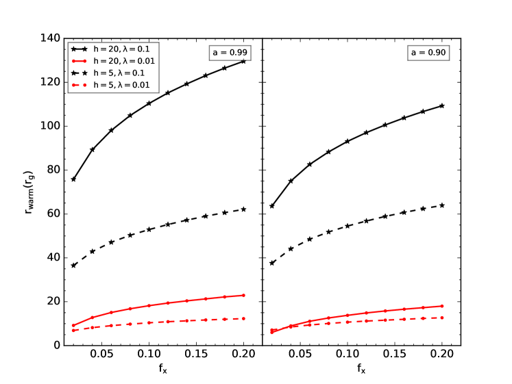
Figure 2: The value of $r_{\mathrm{warm}}$ as a function of the X-ray heating fraction $f_{X}$ for different values of $h$, $\lambda$ and $a$. The reflection and emission spectrum evaluated at $r_{\mathrm{warm}}$ is used to extend the radial integration to $r_{\mathrm{out}}$. For $r<r_{\mathrm{warm}}$ the emission and reflection spectrum is computed for 20 annuli between $r_{\mathrm{in}}$ and $r_{\mathrm{warm}}$. As $r_{\mathrm{warm}}$ is determined by the condition $\xi(r_{\mathrm{warm}})=5$ erg s cm^-1, it is increased by larger values of $f_{X}$ and $\lambda$ (which increases the X-ray flux on the disc), and decreased by a lower $h$ (where light-bending focuses the flux onto the inner disc). There is also a modest drop in $r_{\mathrm{warm}}$ with $a$, in particular at $h=20$, due to a slight decrease in the X-ray luminosity (Eq. 3). There is a weak dependence of $r_{\mathrm{warm}}$ on $h_{f}$ and $\tau$ when $\Gamma>2$ and $\lambda=0.1$, which is not shown in the Figure. In this case, $r_{\mathrm{warm}}$ is lowered by an average of $3.75$% from what is plotted here with a maximum decrease of $12$%.

In all cases, $r_{\mathrm{warm}}$ increases with $f_{X}$, as this parameter is proportional to the flux irradiating the disc (Eq. 3). However, the slope of this relation is smaller for lower values of $\lambda$ (comparing the stars and circles) and $h$ (comparing the solid and dotted lines). In the former case, the lower $\lambda$ significantly enhances the disc density (Eq. 1) which is not compensated by the changes in $f_{X}$. Therefore, $r_{\mathrm{warm}}$ is both smaller and less sensitive to $f_{X}$ for low $\lambda$. In contrast, changes in the lamppost height $h$ affect the radiation pattern on the accretion disc. When $h=5$, for example, light-bending focuses a large fraction of the flux onto the inner accretion disc, and the flux at larger radii is reduced (e.g., Dauser et al., 2013) leading to a smaller $r_{\mathrm{warm}}$ even for large values of $f_{X}$. A larger $h$ provides a more uniform illumination of the disc and so $r_{\mathrm{warm}}$ is largest in this situation. The two panels in Fig. 2 also show that $r_{\mathrm{warm}}$ has a moderate dependence on the black hole spin $a$, in particular when $h=20$ (solid lines), due to $L_{X}$ having a weak dependence on $a$ (Eq. 3).

These values of $r_{\mathrm{warm}}$ broadly separate the disc into regions of ionized refection (when $r<r_{\mathrm{warm}}$) and neutral reflection (when $r>r_{\mathrm{warm}}$). Thus, we expect models with low $r_{\mathrm{warm}}$ (i.e., low $\lambda$) to produce spectra that are dominated by neutral reflection features while those with large $r_{\mathrm{warm}}$ will be dominated by highly ionized reflection. Many models, however, will have a mixture of both due to the ionization gradient across the disc. Since $r_{\mathrm{warm}}$ is determined by the X-ray flux and the disc density, it is nearly independent of the warm corona parameters $\tau$ and $h_{f}$. There is a slight dependence of $r_{\mathrm{warm}}$ on $h_{f}$ and $\tau$ in the $\lambda=0.1$ models that occurs when $\Gamma>2$ and the ionizing power of the irradiating spectrum is weakened. In this regime, $r_{\mathrm{warm}}$ can be reduced from the plotted values by an average of $3.75$%, with a maximum change of $12$%.

Prior to performing the radial integration, each individual spectrum from a disc annulus (from $r$ to $r+dr_{i}$ if $r\leq r_{\mathrm{warm}}$, or from $r$ to $r+dr_{o}$ if $r>r_{\mathrm{warm}}$) is blurred using the relconv_lp convolution model (Dauser et al., 2013) to take into account the relativistic effects seen by a distant observer. The relconv_lp model is passed the same values of $h$, $a$ and $\Gamma$ as the reflection calculation described in Sect. 2.1. We assume isotropic limb darkening and a disc inclination to the line of sight of $i=30^{\circ}$. The blurred spectra are then each multiplied by the proper area of the appropriate annulus using Eq. 4 and then summed to produce the final reXcor model in units of ergs s^-1.

Before examining the resulting spectra in detail, it is important to recognize the limitations of the method presented here. Although the calculation of the spectrum from each annulus extends to $\approx 1$ eV in order to conserve energy (e.g., Ballantyne, 2020), the limited number of elements and low-ionization states treated in the code restricts the accuracy of the predicted spectra at energies $\la 0.1$ keV. In addition, the integrated reXcor model uses the spectrum at $r_{\mathrm{warm}}$ for $r>r_{\mathrm{warm}}$. Therefore, the thermal emission from the disc at these radii will not be properly included in the final spectrum. As a result, the reXcor model should only be used in the X-ray band, at energies $\ga 0.3$ keV. We focus on this energy range in the remainder of the paper. Lastly, the lamppost geometry assumed here is only one possible geometry for the location of the X-ray emitting corona. Other geometries, in particular ones with a truncated accretion disk (e.g. Petrucci et al., 2013; Kubota & Done, 2018), will predict a different ratio of reflection and warm corona emission in the accretion disc spectra than what is produced by reXcor.

2.3 The reXcor grids

The procedure described above produces a single reXcor spectrum given eight parameters: the black hole mass $M$, spin $a$ and accretion rate $\lambda$; the lamppost height $h$ and heating fraction $f_{X}$; the photon index $\Gamma$, and the warm corona heating fraction $h_{f}$ and optical depth $\tau$. As our goal is to construct grids of models to fit to broadband X-ray data, this number of parameters is too large to be practical. In addition, it is not physically plausible for parameters such as $M$ and $\lambda$ to be realistically measured with such a phenomenological model using only X-ray data. Therefore, it is worthwhile examining the dependence of the final spectra on the model parameters to determine which are less important and can be removed from a fitting procedure.

Figure 3 shows how a reXcor model depends on four parameters: $M$, $\lambda$, $h$ and $a$. The solid line in each panel shows the same model with $M=5\times 10^{7}$ M_⊙, $\lambda=0.1$, $h=20$, $a=0.99$, $h_{f}=0.4$, $f_{X}=0.1$, $\Gamma=1.9$ and $\tau=20$.

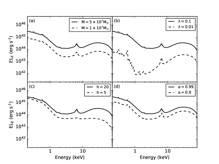
Figure 3: Examples of how a reXcor spectrum changes with black hole mass (a), Eddington ratio (b), lamppost height (c) and black hole spin (d). In each panel the solid line plots a reXcor model with the following parameters: $M=5\times 10^{7}$ M_⊙, $\lambda=0.1$, $h=20$, $a=0.99$, $h_{f}=0.4$, $f_{X}=0.1$, $\tau=20$ and $\Gamma=1.9$. Panel (a) shows that the assumed black hole mass only alters the normalization of the reXcor spectrum. Therefore, the black hole mass is fixed at $5\times 10^{7}$ M_⊙ in all reXcor models. Both $\lambda$ and $h$ significantly affect the shape of the model, but can be broadly separated into "high" and "low" cases (i.e., $\lambda=0.1$, $h=20$ and $\lambda=0.01$, $h=5$). The black hole spin produces a small impact on the amplitude of the reXcor spectrum, and leads to minor changes in the spectral shape due to changes in the relativistic blurring. As a result, reXcor grids are only calculated for $a=0.99$ and $a=0.9$.

We see that changes in the black hole mass $M$ (panel a) impact the normalization of the reXcor spectrum, but has a negligible effect on its shape. This is because the spectral shape is largely determined by the ionization parameter $\xi$ (Eq. 10) which, in this model, is independent of $M$ (Ballantyne, 2017). The change in normalization arises from converting distances from units of $r_{g}$ to physical units, so a smaller $M$ has a physically smaller disc and produces a less luminous spectrum. Since the black hole mass will not impact the determination of the warm corona and reflection parameters (e.g., $h_{f}$ or $f_{X}$) $M$ is fixed at $5\times 10^{7}$ M_⊙ for all reXcor models.

In contrast to the black hole mass, Fig. 3(b,c) show that both $\lambda$ and $h$ significantly affect the final reXcor spectrum. A lower $\lambda$ not only means a smaller X-ray luminosity (Eq. 3), but it also leads to a denser disc (Eq. 1) and therefore a much smaller $\xi$ (Eq. 10). Similarly, decreasing the lamppost height from $h=20$ to $h=5$ greatly increases the illumination of the inner accretion disc due to the effects of light-bending (e.g., Fukumura & Kazanas, 2007; Dauser et al., 2013). Therefore, the disc is much more ionized in the $h=5$ case which leads to very weak reflection features (Ballantyne, 2017). However, rather than having $\lambda$ and $h$ as two additional fit parameters, we produce models that consider "high" and "low" values in both cases. Therefore, reXcor grids are calculated for either $h=20$ or $h=5$. By performing fits with both sets of models, one may be able to determine if the data are best described by a large or a small lamppost height. Likewise, we produce reXcor models for $\lambda=0.1$ or $\lambda=0.01$, as one of these two values should be applicable for a wide range of AGNs (e.g., Vasudevan & Fabian, 2007; Duras et al., 2020).

Lastly, panel (d) of Fig. 3 shows that the black hole spin has a relatively minor impact on the reXcor model. The major effect of spin would be on the ISCO radius of the accretion disc and the level of relativistic blurring suffered by the emitted spectrum. However, when the inner disc is ionized (as is the case in Fig. 3), then the changes in relativistic blurring on the spectrum are very minor. There is also a small drop in normalization when $a$ is lower due to the dependence of $a$ on the proper area element (Eq. 4). Again, to keep the size of the grids manageable, this initial release of reXcor contains grids for $a=0.99$ and $a=0.9$ as these values bracket the majority of spins determined in bright AGNs (Reynolds, 2021).

Table 1 provides a summary of the 8 reXcor grids that are publicly available for use in AGN spectral fitting. The grids contain only the reflection and emission spectra from the accretion disc model described above (see Figs. 4 and 5 below). A separate power-law component (with photon-index tied to the reXcor value) must be included when fitting these models to AGN X-ray data to account for the illuminating spectrum (Sect. 4).

Table 1: There are eight available reXcor grids calculated for two different values of Eddington ratio, black hole spin and lamppost height. The parameters of all grids are listed in Table 2. A black hole mass $M=5\times 10^{7}$ M_⊙ is used in all grids. These table models can be downloaded from the XSPEC website.

Eddington ratio ($\lambda$)	Black hole spin ($a$)	Lamppost height ($h$)	Filename
$0.01$	$0.9$	$5$ $r_{g}$	reXcor_l001_a09_h5.fits
		$20$ $r_{g}$	reXcor_l001_a09_h20.fits
	$0.99$	$5$ $r_{g}$	reXcor_l001_a099_h5.fits
		$20$ $r_{g}$	reXcor_l001_a099_h20.fits
$0.1$	$0.9$	$5$ $r_{g}$	reXcor_l01_a09_h5.fits
		$20$ $r_{g}$	reXcor_l01_a09_h20.fits
	$0.99$	$5$ $r_{g}$	reXcor_l01_a099_h5.fits
		$20$ $r_{g}$	reXcor_l01_a099_h20.fits

3 The rexcor spectral Model

Each of the eight reXcor grids contain 20570 individual spectral models spanning a broad range of $f_{X}$, $\Gamma$, $h_{f}$ and $\tau$ (Table 2). This section describes how these different parameters, which characterize the warm corona and X-ray emitting lamppost in the model, impact the properties of the soft excess and other features in the reXcor spectra. We focus here on the results using the $a=0.99$ grids, and the equivalent figures for two of the $a=0.90$ grids are presented in Appendix A.

Table 2: The reXcor grid parameters. The values of $f_{X}$ covers the range of bolometric corrections observed in many AGNs (Vasudevan & Fabian, 2007, 2009; Duras et al., 2020). The range of $h_{f}$ allows for models with no warm corona heating ($h_{f}=0$) or with dissipationless discs ($h_{f}=0.8$ and $f_{X}=0.2$).

Parameter	Description	Range	Step Size
$f_{X}$	lamppost heating fraction	$0.02\ldots 0.2$	$0.02$
$\Gamma$	photon index of irradiating power-law	$1.7\ldots 2.2$	$0.05$
$h_{f}$	warm corona heating fraction	$0.0\ldots 0.8$	$0.05$
$\tau_{T}$	warm corona Thomson depth	$10\ldots 30$	$2.0$

The top half of Figure 4 plots several example reXcor spectra from the $\lambda=0.1$, $h=20$, $a=0.99$ grid.

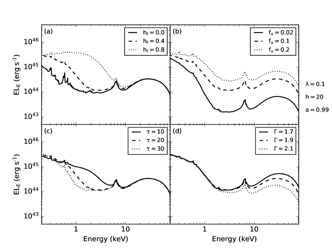
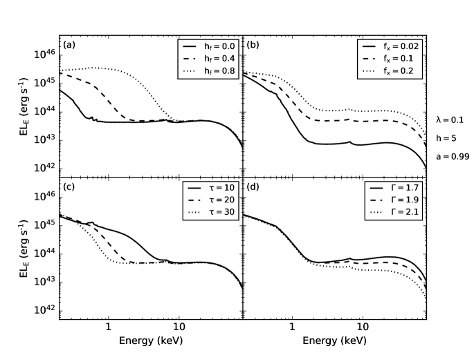
Figure 4: (Top) Examples of reXcor spectra from the grid with $\lambda=0.1$, $h=20$ and $a=0.99$. The dashed line in each panel plots the same spectrum with $h_{f}=0.4$, $f_{X}=0.1$, $\tau=20$, and $\Gamma=1.9$. The different panels show how the spectrum changes to each of these four parameters. A stronger soft excess can be obtained by increasing $h_{f}$ or by decreasing $\tau$ or $f_{X}$. For this value of $\lambda$ and $h$, significant ionized reflection is expected for most spectra. (Bottom) As above, but the spectra are taken from the grid with $\lambda=0.1$ $h=5$ and $a=0.99$. The lower lamppost height produces significant light-bending that enhances the illuminating flux onto the inner accretion disc. The resulting reXcor spectra are dominated by emission from the highly ionized inner accretion disc.

In each panel the dashed line plots the same spectrum with $h_{f}=0.4$, $f_{X}=0.1$, $\tau=20$, and $\Gamma=1.9$, while the other lines show how this baseline model changes due to variations in these four parameters. As expected from Fig. 2, all the spectra in this grid show features associated with ionized reflection, such as an ionized Fe K$\alpha$ line and weak emission features at energies $\la 1$ keV. However, variations in the model parameters can lead to major changes to the overall spectral shape. Panel (a) shows that the strength and smoothness of the soft excess is significantly tied to the value of the warm corona heating fraction $h_{f}$. When $h_{f}=0$, there is no warm coronal heating in the irradiated disc surface, so all the accretion flux is distributed between the thermal blackbody and the X-ray emitting lamppost. In this case, the soft excess is entirely produced by reflection and exhibits emission and absorption features. However, as $h_{f}$ is increased, the gas throughout the layer is heated and maintains a higher ionization state (Ballantyne, 2020). This hotter gas enhances the bremsstrahlung emission from the disc, as well as Comptonizing the blackbody radiation emanating from below, leading to a stronger and smoother soft excess. When $h_{f}=0.8$, the maximum considered in the model, the heating in the disc surface is so large that a Comptonized bremsstrahlung spectrum develops. Thus, the value of $h_{f}$ can lead to a wide variety of soft excess strengths.

The strength of the reflection signal in a reXcor spectrum is driven by $f_{X}$, the hard X-ray heating fraction. As seen in Fig. 4(b), changing $f_{X}$ by an order of magnitude while $h_{f}$ is fixed at $0.4$ has the largest impact at energies $\ga 1$ keV. This means that the relative strength of the soft excess can be reduced by an increase in $f_{X}$. At low values of $f_{X}$, the irradiated gas is less ionized, leading to significant absorption above 1 keV. This absorption is reduced as the gas becomes further ionized at larger values of $f_{X}$ (Ross et al., 1999), leading to a weaker contrast between the soft excess and the higher energy emission. The constant $h_{f}=0.4$ and $\tau=20$ ensures that Comptonization is important in smoothing out features in the soft excess. This panel also shows that changes in $f_{X}$ can be approximated as simply varying the amplitude of the reXcor model. Therefore, because the black hole spin also changes the normalization of the reXcor spectra (Fig. 3(d)), there is a moderate degeneracy between changes in $f_{X}$ and the black hole spin $a$, in the sense that both parameters can adjust the amplitude of the spectrum. For some datasets lacking an independent spin estimate (in particular, those with ionized spectra with few spectral features), statistically similar fits can be obtained with models that have lower spin, but higher $f_{X}$ and models with higher spin, but lower $f_{X}$. With high quality data, this degeneracy could be broken, but, in general, we advise against using reXcor to measure black hole spin.

The optical depth of the warm corona heating layer, $\tau$, also impacts the soft excess (Fig. 4(c)). As the heat injected into the warm corona is fixed, a smaller $\tau$ will spread the heat into a thinner layer, leading to a stronger increase in temperature. A larger $\tau$, in contrast, will yield a cooler corona since the heating is dissipated over a thicker column of gas. These effects can be seen in the three spectra plotted in this panel, as the $\tau=10$ spectrum shows the effects of Comptonization from a hotter gas.

Panel (d) of Fig. 4 illustrates that the photon index $\Gamma$ does not affect the soft excess in the reXcor models, but is crucial in describing the overall hard X-ray spectral shape. Taken together, the combination of these four parameters allows for a wide range of potential AGN spectral shapes, and, through $h_{f}$, quantify the contribution of any warm corona in the X-ray spectrum.

The same patterns in the spectra can be seen in the other reXcor grids, but the spectra are qualitatively different due to changes in the illumination conditions. For example, the bottom half of Fig. 4 plots the same sequence of models as the upper half, but now the lamppost height has been reduced to $h=5$. In this scenario, the extreme light-bending that results from the low lamppost height focuses a large fraction of the flux onto the inner accretion disc making it extremely ionized. The radiation pattern greatly enhances the flux from the inner disc and so the integrated spectrum is dominated by the highly ionized inner regions of the disc. As a result, all the spectra produce a weak ionized Fe K$\alpha$ line that is broadened by both relativistic blurring and strong Comptonization. The $h_{f}=0$ spectrum in panel (a) shows that even with no warm corona, this model produces a smooth soft excess.

The upper-half of Figure 5 shows the reXcor spectra from the $\lambda=0.01$, $h=20$, $a=0.99$ grid.

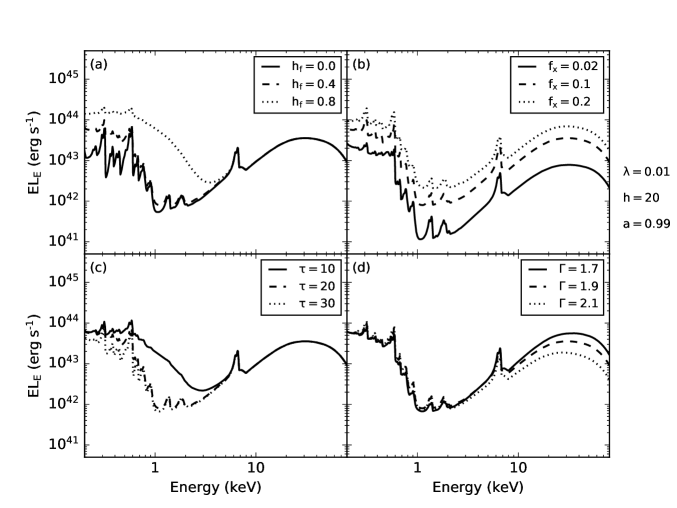
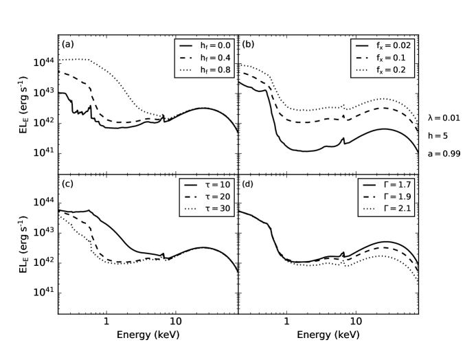
Figure 5: (Top) As in Fig. 4, but the spectra are taken from the grid with $\lambda=0.01$ $h=20$ and $a=0.99$. The smaller $\lambda$ leads to a denser and more weakly illuminated disc. The reXcor spectra are therefore dominated by a low ionization reflector. However, a strong soft excess can still be produced with a sufficiently large $h_{f}$ or small $\tau$. (Bottom) In this case, $h=5$ and the strong light-bending from the low lamppost focuses the radiation onto the inner accretion disc. As a result of the steep ionization gradient on the disc, the reXcor spectra become dominated by neutral reflection close to the black hole (Fig. 2). The soft excess in this situation is then largely formed by the relativistic blurring of these reflection features (e.g., Crummy et al., 2006). However, as when $h=20$, additional warm coronal heating can smooth out and increase the strength of the soft excess.

In contrast to Fig. 4, where $\lambda=0.1$, these spectra frequently exhibit hallmarks of neutral reflection, including a relativistically broadened Fe K$\alpha$ line at 6.4 keV and significant line emission below 1 keV. The smaller $\lambda$ yields a denser and more weakly irradiated disc (Eqs. 1 and 3) which reduces $r_{\mathrm{warm}}$ (Fig. 2). The gas in the disc surface is much cooler in this scenario and produces a soft excess with many emission features. However, as seen in Fig. 5(a,c), a sufficiently large $h_{f}$ in a small enough $\tau$ can raise the gas temperature to the point where a smooth soft excess is generated. In general, it is more challenging for a warm corona to be an important contributor to the soft excess when the gas is denser and can cool more efficiently (Ballantyne, 2020).

When the lamppost height is reduced to $h=5$ (bottom half of Fig. 5), light-bending causes the disc to be strongly illuminated at small radii, but the ionization parameter of the gas remains relatively low (Fig. 2) resulting in reXcor spectra dominated by highly relativistically blurred neutral reflection which significantly contributes to the soft excess (e.g. Crummy et al., 2006). However, as seen in panels (a)-(c) of the figure, additional warm coronal heating is needed in this scenario to strengthen and smooth out the soft excess.

Overall, Figs. 4 and 5 show that the reXcor grids provide spectra that produce a diverse range of spectral shapes, in particular for the soft excess. The combination of relativistically blurred reflection, an ionization gradient along the disc, and warm coronal heating lead to soft excesses with different strengths, slopes and smoothness. Applying a reXcor grid to an AGN dataset will therefore allow an estimate of how the accretion power is distributed within the disc.

4 examining the soft excess in agns with rexcor

In this section we illustrate the use of reXcor in fitting AGN X-ray data and demonstrate how the model can constrain interesting properties of the energy flow in AGN accretion discs. We fit several joint XMM-Newton and NuSTAR spectra of two Seyfert 1 galaxies, HE 1143-1820 and NGC 4593, that exhibit both reflection features and a significant soft excess (Fig. 6). The fits presented below are performed with XSPEC v.12.12.0g (Arnaud, 1996). Uncertainties on the fit parameters are the 90 per cent confident level for a single parameter (i.e., a $\Delta\chi^{2}=2.71$ criterion).

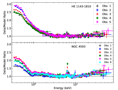
Figure 6: (Top) Data to model ratios found from the five joint XMM-Newton/NuSTAR observations of HE 1143-1820 when fit with a simple absorbed power-law in the energy range $3$–$6$ keV and $7$–$20$ keV and then extrapolated to the full energy band. A prominent Fe K$\alpha$ line, Compton reflection hump and strong soft excess are seen in all observations. (Bottom) As in the other panel, but now showing the results for the six observations of NGC 4593.

4.1 HE 1143-1820

The Seyfert 1 HE 1143-1820 ($z=0.0328$) was monitored by XMM-Newton (Jansen et al., 2001) and NuSTAR (Harrison et al., 2013) with five $20$ ks observations, each separated by two days. The spectral and timing analysis of this dataset was published by Ursini et al. (2020), and we use the same five sets of EPIC-pn (Strüder et al., 2001) and NuSTAR spectra as described in that paper. As reXcor is unable to make predictions at ultraviolet wavelengths, we do not analyze the data from XMM-Newton Optical Monitor (Mason et al., 2001).

The Eddington ratio of HE 1143-1820 is estimated to be $\lambda\sim 0.16$–$0.2$ (Ursini et al., 2020), but the object does not have a detectable broad Fe K$\alpha$ line and does not have a black hole spin measurement. Therefore, we choose the $\lambda=0.1$ and $a=0.99$ series of reXcor grids to fit the data and test both the $h=20$ and $h=5$ cases. In addition to reXcor, the spectral model includes a cutoff power-law (zcutoffpl) and neutral reflection from distant material (xillver; García et al. 2013) which is needed to fit the narrow Fe K$\alpha$ line in the source. The cutoff energy in both of these components is fixed at $100$ keV (Ursini et al., 2020), and the $\Gamma$ is tied to the same value as in the reXcor model. A solar iron abundance and an inclination angle of $30^{\circ}$ are assumed in the xillver model. Neutral absorption due to a Galactic column density of $N_{\mathrm{H}}=3.47\times 10^{20}$ cm^-2 (Kalberla et al., 2005) is included using the phabs model.

The five observations are fit simultaneously with $\Gamma$, $h_{f}$, $f_{X}$, $\tau$, and the normalizations of the 3 spectral components (zcutoffpl, reXcor, and xillver) free to vary for each observation. To simplify the procedure, we ignore the small constant offset between the two NuSTAR focal plane modules (FPMA and FPMB) in each observation (i.e., they are treated as one data group); however, a variable normalization constant is applied to the EPIC-pn data. Finally, as discussed by Ursini et al. (2020), there is a small, energy-dependent offset in $\Gamma$ between XMM-Newton and NuSTAR spectra of the same source. To correct for this, we follow Ursini et al. (2020) and apply a cross-calibration function to the XMM-Newton data proportional to $E^{\Delta\Gamma}$, where $\Delta\Gamma=\Gamma^{\mathrm{XMM}}-\Gamma^{\mathrm{NuSTAR}}$ (Ingram et al., 2017). The results presented below report photon indices and fluxes using the NuSTAR data.

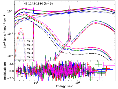
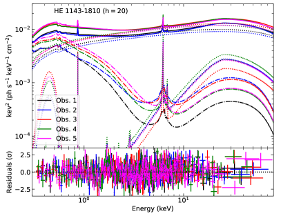
Figure 7: (Left) The upper panel plots the model components predicted from our $h=5$ fit (upper half of Table 3) for each of the 5 observations of HE 1143-1820. The solid lines plot the total model, while the reXcor components are shown as the dot-dashed lines. The dotted lines denote the remaining components of the model (the cutoff power-law, two Gaussian emission line, and xillver). This fit uses the reXcor_l01_a099_h5.fits grid. The lower panel shows the residuals to the fit in units of $\sigma$. (Right) As in the other panel, but for the $h=20$ fit (lower half of Table 3). This fit uses the reXcor_l01_a099_h20.fits grid.

Both the $h=5$ and $20$ reXcor models yield very good fits to the HE 1143-1820 data (with reduced $\chi^{2}\la 1$), and the results are shown in Table 3 and Figure 7.

Table 3: Results from fitting five XMM-Newton and NuSTAR observations of the Seyfert 1 galaxy HE 1143-1820 with the following spectral model: phabs*(zgauss1+zgauss2+zcutoffpl+reXcor+xillver). An energy dependent cross-calibration function proportional to $E^{\Delta\Gamma}$, where $\Delta\Gamma=\Gamma^{\mathrm{XMM}}-\Gamma^{\mathrm{NuSTAR}}$ is included in the model (Ursini et al., 2020). All five observations of the source were fit simultaneously between $0.3$ and $79$ keV. These fits uses the $\lambda=0.1$, $a=0.99$, reXcor grids, with the top half of the table showing the results from the $h=5$ grid ( $\chi^{2}/\mathrm{dof}=1934/1949$) and the lower half gives the results from the $h=20$ set of models ($\chi^{2}/\mathrm{dof}=1928/1949$). The two zgauss components likely arise from N vi and Ne ix, respectively. The latter line is unresolved (with $\sigma$ fixed at $0$ keV). The normalization of the lines ($K$) are in units of ph s^-1 cm^-2, and their equivalent widths are listed as ’EW’. All fluxes ($F$) are tabulated in units of erg s^-1 cm^-2. A ’p’ in the errorbar indicates that the parameter pegged at the upper or lower limit of the grid. The photon-indices and fluxes are derived from the NuSTAR spectra.

		All Obs.	Obs. 1	Obs. 2	Obs. 3	Obs. 4	Obs. 5
	$\log F_{\mathrm{2-10\ keV}}$		$-10.65$	$-10.67$	$-10.55$	$-10.56$	$-10.57$
				$h=5$
zgauss1	$E_{1}$ (keV)	$0.43^{+0.02}_{-0.01}$
	$\sigma_{1}$ (keV)	$0.06\pm 0.02$
	$K_{1}$ ($\times 10^{-3}$)		$0.72\pm 0.03$	$0.67\pm 0.31$	$2.0\pm 0.6$	$1.3\pm 0.5$	$1.5^{+0.4}_{-0.5}$
	EW (eV)		11	11	22	15	15
zgauss2	$E_{2}$ (keV)	$0.90^{+0.02}_{-0.01}$
	$K_{2}$ ($\times 10^{-5}$)		$4.9^{+2.5}_{-2.3}$	$3.3\pm 2.7$	$5.7^{+2.9}_{-3.0}$	$5.6^{+3.2}_{-1.6}$	$5.6^{+3.0}_{-2.7}$
	EW (eV)		4	3	4	4	3
zcutoffpl	$\Gamma$		$1.76^{+0.04}_{-0.03}$	$1.76^{+0.01}_{-0.02}$	$1.75^{+0.02}_{-0.03}$	$1.77\pm 0.03$	$1.75\pm 0.03$
	$\Delta\Gamma$		$-0.042$	$-0.065$	$-0.029$	$-0.045$	$-0.052$
reXcor	$f_{X}$		$0.045^{+0.015}_{-0.006}$	$0.05\pm 0.01$	$0.060\pm 0.007$	$0.052\pm 0.012$	$0.05\pm 0.01$
	$h_{f}$		$0.45\pm 0.09$	$0.39\pm 0.05$	$0.45^{+0.1}_{-0.07}$	$0.45^{+0.14}_{-0.08}$	$0.45^{+0.01}_{-0.04}$
	$\tau$		$11.6^{+1.4}_{-1.0}$	$10.2^{+0.8}_{-0.2p}$	$11.3^{+0.6}_{-0.8}$	$11.1^{+1.2}_{-0.8}$	$10.4^{+0.6}_{-0.4p}$
	$\log F_{\mathrm{0.3-10\ keV}}^{\mathrm{PL}}$		$-10.42\pm 0.01$	$-10.45\pm 0.01$	$-10.33\pm 0.01$	$-10.33\pm 0.01$	$-10.35^{+0.01}_{-0.003}$
	$\log F_{\mathrm{0.3-10\ keV}}^{\mathrm{reXcor}}$		$-10.90^{+0.06}_{-0.05}$	$-10.88^{+0.05}_{-0.06}$	$-10.72^{+0.06}_{-0.05}$	$-10.75^{+0.05}_{-0.06}$	$-10.65^{+0.04}_{-0.03}$
	$\log F_{\mathrm{0.3-10\ keV}}^{\mathrm{xillver}}$		$-12.08^{+0.09}_{-0.10}$	$-11.99^{+0.05}_{-0.08}$	$-12.12^{+0.09}_{-0.14}$	$-11.96^{+0.09}_{-0.11}$	$-12.07\pm 0.10$
	$\chi^{2}/\mathrm{dof}$	$1934/1949$
				$h=20$
zgauss1	$E_{1}$ (keV)	$0.44^{+0.02}_{-0.03}$
	$\sigma_{1}$ (keV)	$0.06\pm 0.02$
	$K_{1}$ ($\times 10^{-3}$)		$0.62^{+0.04}_{-0.03}$	$0.56^{+0.04}_{-0.03}$	$1.7^{+1}_{-0.5}$	$1.2^{+0.7}_{-0.4}$	$1.4^{+0.8}_{-0.6}$
	EW (eV)		10	9	21	15	16
zgauss2	$E_{2}$ (keV)	$0.89^{+0.01}_{-0.02}$
	$K_{2}$ ($\times 10^{-5}$)		$5.7^{+2.7}_{-2.4}$	$5.7^{+3.1}_{-3.3}$	$7.0\pm 3.7$	$6.6^{+4.2}_{-3.5}$	$6.4^{+3.5}_{-3.4}$
	EW (eV)		5	5	4	4	4
zcutoffpl	$\Gamma$		$1.76^{+0.04}_{-0.03}$	$1.76\pm 0.02$	$1.73^{+0.03}_{-0.02}$	$1.77^{+0.03}_{-0.04}$	$1.75^{+0.03}_{-0.02}$
	$\Delta\Gamma$		$-0.040$	$-0.056$	$-0.024$	$-0.042$	$-0.047$
reXcor	$f_{X}$		$0.028^{+0.025}_{-0.008p}$	$0.051^{+0.011}_{-0.016}$	$0.050^{+0.021}_{-0.020}$	$0.038^{+0.024}_{-0.018p}$	$0.033^{+0.018}_{-0.013p}$
	$h_{f}$		$0.50^{+0.06}_{-0.08}$	$0.36^{+0.14}_{-0.07}$	$0.49^{+0.08}_{-0.13}$	$0.50^{+0.08}_{-0.14}$	$0.52^{+0.04}_{-0.09}$
	$\tau$		$12.1^{+1.8}_{-0.8}$	$10.4^{1.5}_{-0.4p}$	$11.9^{+1.5}_{-1.1}$	$11.8^{+1.3}_{-0.7}$	$11.1^{+0.6}_{-0.5}$
	$\log F_{\mathrm{0.3-10\ keV}}^{\mathrm{PL}}$		$-10.42\pm 0.01$	$-10.46\pm 0.01$	$-10.34^{+0.01}_{-0.02}$	$-10.33\pm 0.02$	$-10.36\pm 0.01$
	$\log F_{\mathrm{0.3-10\ keV}}^{\mathrm{reXcor}}$		$-10.90\pm 0.06$	$-10.86\pm 0.05$	$-10.71\pm 0.06$	$-10.76^{+0.08}_{-0.06}$	$-10.66^{+0.06}_{-0.05}$
	$\log F_{\mathrm{0.3-10\ keV}}^{\mathrm{xillver}}$		$-12.13^{+0.13}_{-0.17}$	$-12.12^{+0.11}_{-0.15}$	$-12.32^{+0.19}_{-0.32}$	$-12.02^{+0.12}_{-0.18}$	$-12.15^{+0.13}_{-0.18}$
	$\chi^{2}/\mathrm{dof}$	$1928/1949$

We first focus on the best fit values for the three reXcor parameters that describe the distribution of accretion energy between the warm and hot coronas (i.e., $h_{f}$, $f_{X}$ and $\tau$). The values of these parameters do not significantly differ between the $h=5$ and $h=20$ models. Thus, while we are unable to place a constraint on the lamppost height, the properties of the soft excess in HE 1143-1820 allow a robust measurement of the warm corona properties. Notably, we find that $h_{f}\neq 0$ in all five observations which indicates that warm corona heating is required to account for the soft excess in HE 1143-1820. The optical depth of the warm corona is consistently low and varies only from $\approx 10$ to $\approx 12$. These values are slightly less than those inferred by Ursini et al. (2020) (where $\tau\approx 17.5$) using a model which describes the soft excess with only a Comptonization spectrum. As seen in Fig. 4, a low value of $\tau$ maximizes the heating effects for a given $h_{f}$, and will lead to a stronger and smoother soft exess, as observed in HE 1143-1820. The values of $f_{X}$ indicate that $\la 6$% of the accretion energy is dissipated in the lamppost corona, consistent with the observed bolometric corrections in AGNs at these Eddington ratios (e.g., Duras et al., 2020).

Interestingly, each fit requires the addition of 2 Gaussian emission line components, a broadened one ($\sigma=0.06$ keV) at $\approx 0.43$ keV and an unresolved ($\sigma=0$ keV) at $\approx 0.9$ keV. The lines are highly statistically significant (with F-test probabilities $\ll 10^{-7}$), but have equivalent widths (EWs) of $3$–$22$ eV. The energy of the broadened $0.43$ keV line is consistent with the N vi triplet, and its EW increases from $11$ eV to $22$ eV as the source brightens. This fact, combined with its width, suggests that this line is responding to the changing ionization state of the inner accretion disc. The soft excess produced by reXcor is comprised of blurred ionized reflection superimposed on a Comptonized continuum enhanced by the warm corona. The reXcor spectra include emission from N vi, but appears to underestimate its strength in HE 1143-1820 by $\approx 10$%. This mismatch is likely a result of fact that transitions in He-like ions such as N vi are very sensitive to the temperature, density and optical depth of a plasma (Porquet et al., 2010), and these conditions are not correctly described by the reXcor models for HE 1143-1820. In contrast, the EW of the narrow $0.9$ keV line is roughly constant across all observations, indicating that it originates from an unchanging ionized zone at some distance from the black hole. The line energy is consistent with arising from Ne ix, which is not included in the reXcor model, and therefore this line had to be included as a separate component in the fits. The presence of these emission lines is evidence that the soft excess in HE 1143-1820 is comprised, in part, from photoionized emission across a range of ionization states. Therefore, given the complexity of emission features in this energy range, combined with the available number of lines predicted by reXcor, we expect that the need to add additional Gaussian components will be common when applying reXcor to AGN data.

As the five observations of HE 1143-1820 span a factor of $\approx 2$ in flux, it is interesting to consider how the reXcor parameters change as the source changed in brightness. Panels (a)–(c) of Figure 8 plot $\tau$, $h_{f}$ and $f_{X}$ as a function of the observed $2$–$10$ keV flux of HE 1143-1820 for both the $h=5$ (black circles) and $h=20$ (red triangles) fits.

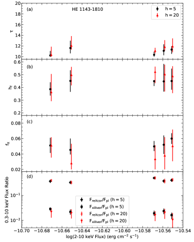
Figure 8: Panels (a) (b) and (c) plot the best-fit values of $\tau$, $h_{f}$ and $f_{X}$ from the reXcor fits to HE 1143-1820 (Table 3 and Fig. 7) against the observed $2$–$10$ keV flux. The results from the $h=5$ model are shown as the black circles, while the red triangles plot the parameters from the $h=20$ model. The lower panel shows that the fraction of the flux described by both the reXcor and xillver models remains relatively unchanged in each of the five observations for both the $h=5$ and $h=20$ models.

There is no evidence for a correlation (i.e., a linear fit returns a slope consistent with zero) between the these parameters and the observed flux in either scenario. Although an increase in the optical depth with flux is a common prediction of accretion disc models (e.g., Svensson & Zdziarski, 1994; Jiang et al., 2019b), the exact dependence remains uncertain and it is not obvious if such a relationship extends to the warm corona. These results are consistent with the fits of Ursini et al. (2020) using a Comptonization model. It is possible that observations spanning a larger range in flux are necessary to detect variations in these parameters.

The normalization of the reXcor models is determined by many quantities, including the distance to the source, the area of the disc emission region, the inclination angle of the disc, the black hole mass and spin, and the geometry of the X-ray source. As it is impractical to unravel all these effects to interpret the normalization returned by the fits, we consider the ratio of the reXcor and power-law fluxes. The scenario used to calculate reXcor spectra would predict a ratio close to unity, as the flux from the disc is produced by reprocessing the luminosity of the lamppost (Sect. 2). However, this ratio could be significantly altered by effects not included in our model, such as a non-stationary X-ray emitting corona (e.g., Beloborodov, 1999), a truncated accretion disc (e.g., Kubota & Done, 2018), or a non-flat disc surface that could enhance the overall reflection strength (e.g. Fabian et al., 2002). Fig. 8(d) shows that the total reXcor flux (in the $0.3$–$10$ keV band) in the HE 1143-1820 fits is a factor of $\approx 0.4$ of the power-law flux, independent of the assumed coronal height. This flux ratio could be explained by a moderately outflowing corona (Beloborodov, 1999) or a truncated disc. Finally, we find that the flux of the xillver model is $\approx 0.02\times$ less than the power-law flux between $0.3$–$10$ keV because of the very small albedo of dense, neutral gas in this energy range.

4.2 NGC 4593

As a second example, we apply the reXcor model to NGC 4593 ($z=0.0831$), a Seyfert 1 with $\lambda\approx 0.04$ (Vasudevan & Fabian, 2009). Similar to HE 1143-1820, NGC 4593 has five coordinated $20$ ks XMM-Newton and NuSTAR observations that span a factor of $\approx 2$ in flux (Ursini et al., 2016; Middei et al., 2019). The first observation caught the source rapidly declining in flux, and so Ursini et al. (2016) split this observation into two in order to isolate the low count-rate region which exhibits a hard spectral shape. The resulting six EPIC-pn and NuSTAR spectra are analyzed here.

We apply a similar spectral model to NGC 4593 as with HE 1143-1820: neutral absorption with phabs ($N_{H}=1.89\times 10^{22}$ cm^-2; Kalberla et al. 2005), a neutral xillver model to account for distant reflection, a cutoff power-law, and reXcor. Given the lower Eddington ratio in this source, we use the $\lambda=0.01$ reXcor grids. Although the source shows evidence for a broadened Fe K$\alpha$ line (Brenneman et al., 2007; Ursini et al., 2016), a spin estimate does not exist. Therefore, we begin our analysis with the $a=0.99$ reXcor grids, but also test the result with the $a=0.9$ grids. In addition, NGC 4593 has been previously fit with two warm absorbers (Brenneman et al., 2007; Ursini et al., 2016) and a photoionized emitter (Ursini et al., 2016) to account for the observed soft X-ray spectral complexity. Therefore, we include a warm absorber table model calculated with XSTAR (Walton et al., 2013) in our fit, but we find that a distinct photoionized plasma emission model is not required. In contrast with the HE 1143-1820 fits, the cutoff energy of the zcutoffpl model (which is tied to the corresponding parameter in xillver) is allowed to vary in each observation as Ursini et al. (2016) found that the cutoff energy is large and variable in these observations. Similarly, the iron abundance of the xillver model is allowed to vary, although the value is the same for all observations.

The fit procedure for NGC 4593 is the same as for HE 1143-1820, including the use of the $\Delta\Gamma$ cross-calibration function to account for the small offset in the XMM-Newton and NuSTAR photon indices. As before, we report fluxes and $\Gamma$ from the NuSTAR data. The best fit model (with $\chi^{2}/\mathrm{dof}=2450/2271$) is obtained with the reXcor_l001_a099_h20.fits grid and is shown in Figure 9 with the results tabulated in Table 4.

Table 4: Results from fitting five XMM-Newton and NuSTAR observations of the Seyfert 1 galaxy NGC 4593 with the following spectral model: phabs*WA*(zgauss1+zgauss2+zcutoffpl+reXcor+xillver), where WA denotes a warm absorber table model (Walton et al., 2013). An energy dependent cross-calibration function proportional to $E^{\Delta\Gamma}$, where $\Delta\Gamma=\Gamma^{\mathrm{XMM}}-\Gamma^{\mathrm{NuSTAR}}$ is included in the model (Ursini et al., 2020). The first observation is split in two (e.g., Ursini et al., 2016) and all six spectra are fit simultaneously between $0.3$ and $79$ keV. This fit uses the $\lambda=0.01$, $a=0.99$, $h=20$ reXcor grid. The two zgauss components have $\sigma=0$ keV with normalizations ($K$) in units of ph s^-1 cm^-2. All fluxes ($F$) are tabulated in units of erg s^-1 cm^-2. A ’p’ in the errorbar indicates that the parameter pegged at the upper or lower limit of the grid. The photon-indices and fluxes are derived from the NuSTAR spectra.

		All Obs.	Obs. 1a	Obs. 1b	Obs. 2	Obs. 3	Obs. 4	Obs. 5
WA	$N_{\mathrm{H}}$ ($\times 10^{21}$ cm-2)	$2.75^{+0.38}_{-0.39}$
	$\log\xi$ (erg s cm-1)	$2.33^{+0.06}_{-0.05}$
xillver	$A_{\mathrm{Fe}}$	$2.7^{+0.5}_{-0.2}$
zgauss1	$E_{1}$ (keV)	$0.47\pm 0.01$
	$K_{1}$ ($\times 10^{-4}$)		$3.6^{+2.1}_{-2.6}$	$0.02{+3}_{-0.2p}$	$2^{+1}_{-1.9}$	$0.01^{+2}_{-0.01p}$	$3.4^{+1.7}_{-2.5}$	$2.2^{+3.0}_{-1.1}$
	EW (eV)		10	0	11	0	9	5
zgauss2	$E_{2}$ (keV)	$0.65\pm 0.01$
	$K_{2}$ ($\times 10^{-4}$)		$1.7^{+0.8}_{-0.7}$	$1.1^{+0.5}_{-0.7}$	$0.7^{+0.2}_{-0.4}$	$1.2\pm 0.4$	$2.1^{+0.7}_{-0.8}$	$2.3^{+0.3}_{-1}$
	EW (eV)		9	6	7	12	10	11
zcutoffpl	$\Gamma$		$1.84\pm 0.04$	$1.82^{+0.03}_{-0.06}$	$1.76^{+0.05}_{-0.01}$	$1.75^{+0.04}_{-0.03}$	$1.84^{+0.02}_{-0.03}$	$1.84\pm 0.03$
	$E_{\mathrm{cut}}$ (keV)		$>240$	$>210$	$>140$	$>240$	$>700$	$>410$
	$\Delta\Gamma$		$-0.025$	$-0.065$	$-0.065$	$-0.045$	$-0.021$	$-0.016$
reXcor	$f_{X}$		$0.060^{+0.14p}_{-0.040p}$	$0.02^{+0.066}_{-0p}$	$0.02^{+0.067}_{-0p}$	$0.029^{+0.152}_{-0.008}$	$0.060^{+0.098}_{-0.040p}$	$0.021^{+0.1}_{-0.001p}$
	$h_{f}$		$0.50^{+0.13}_{-0.19}$	$0.50^{+0.19}_{-0.23}$	$0.38^{+0.10}_{-0.23}$	$0.47^{+0.21}_{-0.38}$	$0.60^{+0.11}_{-0.15}$	$0.45^{+0.23}_{-0.21}$
	$\tau$		$22.2^{+7.8p}_{-8.2}$	$24.5^{+5.5p}_{-10.8}$	$30^{+0p}_{-14.3}$	$27.8^{+2.2p}_{-17.6}$	$28.1^{+1.9p}_{-9.8}$	$23.4^{+6.6p}_{-4.8}$
	$\log F_{\mathrm{0.3-10\ keV}}^{\mathrm{PL}}$		$-10.34^{+0.02}_{-0.01}$	$-10.41\pm 0.01$	$-10.58\pm 0.01$	$-10.58\pm 0.01$	$-10.31\pm 0.01$	$-10.31\pm 0.01$
	$\log F_{\mathrm{0.3-10\ keV}}^{\mathrm{reXcor}}$		$-11.52^{+0.07}_{-0.06}$	$-11.59^{+0.07}_{-0.08}$	$-11.70^{+0.06}_{-0.05}$	$-11.69^{+0.05}_{-0.08}$	$-11.46^{+0.04}_{-0.05}$	$-11.47^{+0.04}_{-0.06}$
	$\log F_{\mathrm{0.3-10\ keV}}^{\mathrm{xillver}}$		$-12.07^{+0.10}_{-0.16}$	$-11.96^{+0.09}_{-0.14}$	$-12.02\pm 0.08$	$-11.96\pm 0.10$	$-11.89\pm 0.08$	$-11.95^{+0.05}_{-0.10}$
	$\log F_{\mathrm{2-10\ keV}}$		$-10.6$	$-10.66$	$-10.8$	$-10.79$	$-10.5644$	$-10.5645$
	$\chi^{2}/\mathrm{dof}$	$2450/2271$

The $h=5$ grid yields a worse fit ($\chi^{2}/\mathrm{dof}=2472/2271$), with similar average values of $f_{X}$ and $h_{f}$ as the $h=20$ model. The average value of $\tau$ drops from $26$ with the $h=20$ grid to $17$ with the $h=5$ models. Overall, it appears that a higher coronal height is preferred in NGC 4593. However, fits using $a=0.9$ grids do not appreciably change the goodness of fit compared to the $a=0.99$ grids, so we are unable to provide a constraint on the black hole spin. Interestingly, the best-fit model requires only a single, moderately ionized warm absorber. When a second warm absorber was added to the model, its column density was driven to very low values, effectively eliminating any impact on the spectrum.

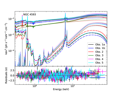
Figure 9: The upper panel plots the model components predicted from our best fit (Table 4) for each of the 6 observations of NGC 4593. The solid lines plot the total model, while the reXcor components are shown as the dot-dashed lines. The dotted lines denote the remaining components of the model (the cutoff power-law, two Gaussian emission lines, and xillver). This model uses the reXcor_l001_a099_h20.fits grid. The lower panel shows the residuals to the fit in units of $\sigma$.

The reXcor spectra in the NGC 4593 fit show many features of reflection from a weakly ionized accretion disc. This is a result of the $\lambda=0.01$, $h=20$ grid which naturally produces spectra with a relatively small ionized zone (Fig. 2). Nevertheless, Table 4 shows that $h_{f}\sim 0.5$ in all observations which indicates that warm corona heating is necessary to satisfactorily account for the observed soft excess. Fig. 5(a) shows that heating at this level typically raises the soft emission at energies $\la 1$ keV. The warm corona depth in NGC 4593 are typically quite large with $\tau\ga 20$ and hitting the upper-limit of $30$ in each observation. A large value of $\tau$ for the warm corona is consistent with the fits of Middei et al. (2019) using a Comptonization model. As discussed in Sect. 3, a large value of $\tau$ spreads out the heat from a given $h_{f}$ which will limit the temperature increase in the corona. The average value of $\tau$ found for NGC 4593 is $26$, much larger than the mean $\tau$ of $11$ measured in the higher $\lambda$ HE 1143-1820 with a stronger and smoother soft excess. Finally, we find that the value of $f_{X}$ in NGC 4593 is frequently consistent with the lower limit of the grids, $f_{X}\sim 0.02$, indicating that the lamp-post is receiving a small fraction of the accretion power.

Fig. 9 shows that the soft excess predicted by the reXcor model is imprinted with several broadened emission features arising from reflection off the disc. This structured soft excess appears to eliminate the need for a second warm absorber component, as well as the photoionized emitter, that was used in earlier models (Brenneman et al., 2007; Ursini et al., 2016). The need for these additional models likely was a result of assuming a smooth spectral model for the soft excess (such as a Comptonized model, or a bremsstrahlung spectrum). However, the reXcor model naturally includes both photoionized and Comptonized emission, in addition to bremsstrahlung, and therefore yields a more straightforward model of the spectrum.

As in HE 1143-1820, two Gaussian emission lines are needed in the final model, but, in this case, both lines are narrow. The lower-energy line (at $0.46$ keV) is weak (with a normalization consistent with zero in Obs. 1b and 3), and could be associated with a blend of the Ly$\beta$ line and the radiative recombination continuum from C vi. The $0.65$ keV line is likely O viii Ly$\alpha$, and is also weak with an EW$\sim 10$ eV. These lines will originate in distant ionized gas not connected to the reXcor model.

The top three panels of Figure 10 shows how the three reXcor parameters vary with the observed $2$–$10$ keV flux of NGC 4593.

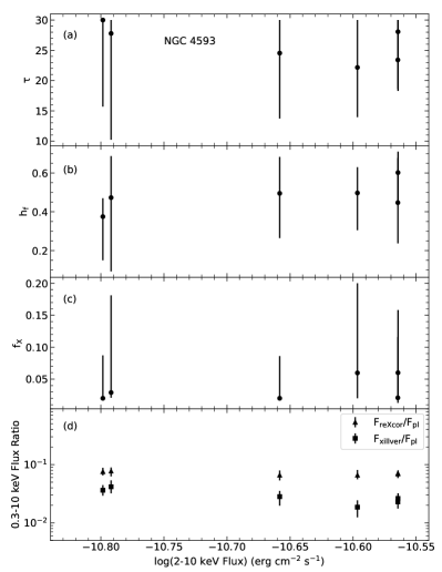
Figure 10: As in Fig. 8, but now plotting the results from our fits to NGC 4593 (Table 4).

Similar to HE 1143-1820, none of the parameters show any correlations with the observed flux. Fig. 10(d) shows the flux ratios of the reXcor and xillver model components relative to the power-law model. The reXcor $0.3$–$10$ keV flux is consistently $\approx 7$% of the power-law flux, while the xillver flux varies between $2$ and $4$% of the power-law. This low value of the reXcor flux ratio is largely due to the low ionization state of the inner accretion disc. X-rays absorbed at $\ga 1$ keV will be thermalized and re-emitted at $<0.3$ keV (e.g., Ross et al., 1999), leading to a reduction in the reXcor flux ratio. As the disc becomes more ionized, fewer hard X-rays can be absorbed and reprocessed in this way. This effect likely explains the lower reXcor ratio found in the NGC 4593 fits compared to those for HE 1143-1820 (Fig. 8).

5 Summary

This paper introduces a new phenomenological spectral model of AGNs, reXcor, that self-consistently combines the effects of a warm corona with the X-ray reflection spectrum from the inner $400$ $r_{g}$ of an accretion disc. The goal of reXcor is to simultaneously fit both the relativistic reflection signal and the soft excess in AGNs. The model assumes the disc is irradiated by a lamppost X-ray source, and takes into account relativistic light-bending and the ionization gradient on the surface of the disc. To produce a warm corona, accretion energy is injected into the irradiated disc surface, altering the emission and reflection spectrum due to enhanced Comptonization and bremsstrahlung emission. The flux released in the lamppost, the warm corona, and the bulk of the accretion disc must sum to the total local dissipation rate. reXcor spectra can be used to model AGN spectra at energies $\ga 0.3$ keV.

In this initial release, a total of 8 reXcor table models are available (Table 1), separated by specific values of the lamppost height ($h$), the accretion rate ($\lambda$), and the black hole spin ($a$). Each table model contains 20570 reXcor spectra (Table 2) that are parameterized by the photon-index of the irradiating spectrum ($\Gamma$), the lamppost heating fraction ($f_{X}$), and the warm corona heating fraction ($h_{f}$) and Thomson depth ($\tau$). These last three parameters describe changes in the warm corona properties and the distribution of energy in the accretion disc. As a result, varying $h_{f}$, $f_{X}$ and $\tau$ lead to wide range of possible soft excess shapes and sizes (Sect. 3).

We illustrate the use of reXcor by showing fits to the joint XMM-Newton and NuSTAR monitoring campaigns of the Seyfert 1s HE 1143-1820 and NGC 4593 (Sect. 4). The reXcor model provides a good fit to the soft excess in both AGNs with $h_{f}\approx 0.5$, indicating that a warm corona is an important contributor to the soft excess in both sources. The optical depth of the warm corona is much higher ($\tau\approx 26$) in the low Eddington ratio AGN NGC 4593 than in more rapidly accreting HE 1143-1820 ($\tau\approx 11)$. Examining this relationship, and searching for others, using a wide range of AGNs will lead to new insights into how the energy of the accretion flow is distributed in AGNs. In contrast, it appears to be challenging to use reXcor grids to provide robust constraints on the black hole spin or the height of the lamppost corona without additional information (e.g., spectral-timing analysis from STROBE-X observations Ray et al. 2019). However, the derived warm corona parameters of HE 1143-1820 and NGC 4593 are largely insensitive to changes in either $h$ or $a$. Thus, reXcor may be confidently used to determine the warm corona properties of AGNs that lack a black hole spin measurement or an estimate of the coronal height.

Compelling evidence now exists that the soft excess in AGNs can be explained by the combination of relativistic reflection from the accretion disc with Comptonization in a warm corona (e.g., Xu et al., 2021b). Systematic use of the reXcor model will allow for a comprehensive test of this idea. reXcor is designed for use with any broadband AGN X-ray spectrum with a good soft X-ray response, including future observations by XRISM (XRISM Science Team, 2020), Athena (Nandra et al., 2013), and, potentially, STROBE-X (Ray et al., 2019). We expect that the application of reXcor to both archival and future datasets may finally lead to an improved understanding of the soft excess puzzle in AGNs. Future planned releases of reXcor will include a wider range of black hole spins, plus the ability to consider non-Solar abundances.

Data Availability

The data underlying this article will be shared on reasonable request to the corresponding author. The reXcor models are publicly available through the XSPEC website.

Appendix A Additional Examples from the reXcor Grids

We present examples of the reXcor model spectra from two of the $a=0.90$ grids. The lower black hole spin increases the radius of the ISCO and reduces the amount of relativistic blurring impacting the model spectra. As a result, the largest impact on the reXcor models is on the spectra that emerge from the inner disc. However, the inner disc is highly ionized when $\lambda=0.1$ (Fig. 2), so the largest impact of the lower spin occurs in the $\lambda=0.01$ reXcor models (Fig. 11.)

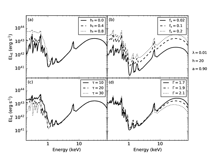
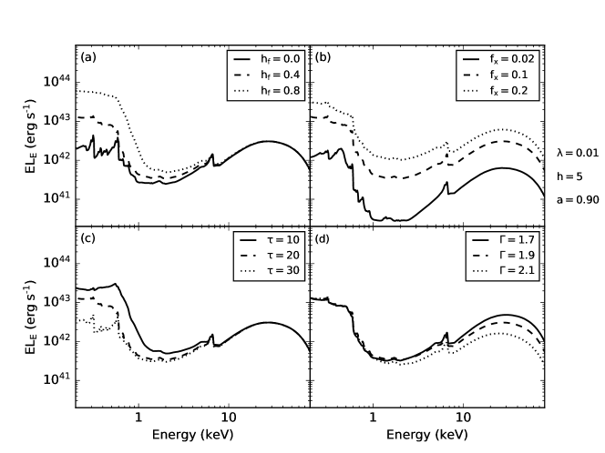
Figure 11: As in Fig. 4, but the spectra are taken from the grid with $\lambda=0.01$ and $a=0.90$. The top figure shows the results with $h=20$ and the lower one plots models with $h=5$. The smaller spin leads to less relativistic blurring when compared to the equivalent $a=0.99$ spectra in Fig. 5.

Comparing the spectra shown in this figure to the corresponding ones in Fig. 5, shows that that the lower spin reduces the blurring of the reflection features. In addition, the lower spin somewhat reduces the luminosity of the lamppost (Eq. 3), which leads to a drop in the ionization state of the disc. Therefore, the $a=0.9$ spectra have a larger contribution from neutral reflection in the final model. As mentioned in Sect. 3, the drop in the the reXcor amplitude due to a lower $a$ can be compensated, in part, by increasing $f_{X}$. This degeneracy limits the ability to use reXcor to constrain black hole spin. The effects of the warm corona parameters (e.g., $h_{f}$, $\tau$) are unaffected by the lower spin.

References

- Arnaud (1996) Arnaud K. A., 1996, in Jacoby G. H., Barnes J., eds, Astronomical Society of the Pacific Conference Series Vol. 101, Astronomical Data Analysis Software and Systems V. p. 17
- Ballantyne (2017) Ballantyne D. R., 2017, MNRAS, 472, L60
- Ballantyne (2020) Ballantyne D. R., 2020, MNRAS, 491, 3553
- Ballantyne & Xiang (2020) Ballantyne D. R., Xiang X., 2020, MNRAS, 496, 4255
- Ballantyne et al. (2001) Ballantyne D. R., Ross R. R., Fabian A. C., 2001, MNRAS, 327, 10
- Beloborodov (1999) Beloborodov A. M., 1999, ApJ, 510, L123
- Bianchi et al. (2009) Bianchi S., Guainazzi M., Matt G., Fonseca Bonilla N., Ponti G., 2009, A&A, 495, 421
- Brenneman et al. (2007) Brenneman L. W., Reynolds C. S., Wilms J., Kaiser M. E., 2007, ApJ, 666, 817
- Cackett et al. (2021) Cackett E. M., Bentz M. C., Kara E., 2021, iScience, 24, 102557
- Crummy et al. (2006) Crummy J., Fabian A. C., Gallo L., Ross R. R., 2006, MNRAS, 365, 1067
- Dauser et al. (2013) Dauser T., Garcia J., Wilms J., Böck M., Brenneman L. W., Falanga M., Fukumura K., Reynolds C. S., 2013, MNRAS, 430, 1694
- De Marco et al. (2013) De Marco B., Ponti G., Cappi M., Dadina M., Uttley P., Cackett E. M., Fabian A. C., Miniutti G., 2013, MNRAS, 431, 2441
- Duras et al. (2020) Duras F., et al., 2020, arXiv e-prints, p. arXiv:2001.09984
- Fabian & Ross (2010) Fabian A. C., Ross R. R., 2010, Space Sci. Rev., 157, 167
- Fabian et al. (2002) Fabian A. C., Ballantyne D. R., Merloni A., Vaughan S., Iwasawa K., Boller T., 2002, MNRAS, 331, L35
- Fukumura & Kazanas (2007) Fukumura K., Kazanas D., 2007, ApJ, 664, 14
- García et al. (2013) García J., Dauser T., Reynolds C. S., Kallman T. R., McClintock J. E., Wilms J., Eikmann W., 2013, ApJ, 768, 146
- García et al. (2019) García J. A., et al., 2019, ApJ, 871, 88
- Gierliński & Done (2004) Gierliński M., Done C., 2004, MNRAS, 349, L7
- Gliozzi & Williams (2020) Gliozzi M., Williams J. K., 2020, MNRAS, 491, 532
- Gronkiewicz & Różańska (2020) Gronkiewicz D., Różańska A., 2020, A&A, 633, A35
- Harrison et al. (2013) Harrison F. A., et al., 2013, ApJ, 770, 103
- Ingram et al. (2017) Ingram A., van der Klis M., Middleton M., Altamirano D., Uttley P., 2017, MNRAS, 464, 2979
- Jansen et al. (2001) Jansen F., et al., 2001, A&A, 365, L1
- Jiang et al. (2019a) Jiang J., et al., 2019a, MNRAS, 489, 3436
- Jiang et al. (2019b) Jiang Y.-F., Blaes O., Stone J. M., Davis S. W., 2019b, ApJ, 885, 144
- Jiang et al. (2020) Jiang J., Gallo L. C., Fabian A. C., Parker M. L., Reynolds C. S., 2020, MNRAS, 498, 3888
- Kalberla et al. (2005) Kalberla P. M. W., Burton W. B., Hartmann D., Arnal E. M., Bajaja E., Morras R., Pöppel W. G. L., 2005, A&A, 440, 775
- Kara et al. (2016) Kara E., Alston W. N., Fabian A. C., Cackett E. M., Uttley P., Reynolds C. S., Zoghbi A., 2016, MNRAS, 462, 511
- Keek & Ballantyne (2016) Keek L., Ballantyne D. R., 2016, MNRAS, 456, 2722
- Kubota & Done (2018) Kubota A., Done C., 2018, MNRAS, 480, 1247
- Laha & Ghosh (2021) Laha S., Ghosh R., 2021, ApJ, 915, 93
- Magdziarz et al. (1998) Magdziarz P., Blaes O. M., Zdziarski A. A., Johnson W. N., Smith D. A., 1998, MNRAS, 301, 179
- Martocchia & Matt (1996) Martocchia A., Matt G., 1996, MNRAS, 282, L53
- Mason et al. (2001) Mason K. O., et al., 2001, A&A, 365, L36
- Matt et al. (1991) Matt G., Perola G. C., Piro L., 1991, A&A, 247, 25
- Matt et al. (2014) Matt G., et al., 2014, MNRAS, 439, 3016
- Mehdipour et al. (2015) Mehdipour M., et al., 2015, A&A, 575, A22
- Middei et al. (2018) Middei R., et al., 2018, A&A, 615, A163
- Middei et al. (2019) Middei R., et al., 2019, MNRAS, 483, 4695
- Middei et al. (2020) Middei R., et al., 2020, A&A, 640, A99
- Miniutti & Fabian (2004) Miniutti G., Fabian A. C., 2004, MNRAS, 349, 1435
- Nandra et al. (2013) Nandra K., et al., 2013, arXiv e-prints, p. arXiv:1306.2307
- Petrucci et al. (2001) Petrucci P. O., et al., 2001, ApJ, 556, 716
- Petrucci et al. (2013) Petrucci P. O., et al., 2013, A&A, 549, A73
- Petrucci et al. (2018) Petrucci P. O., Ursini F., De Rosa A., Bianchi S., Cappi M., Matt G., Dadina M., Malzac J., 2018, A&A, 611, A59
- Petrucci et al. (2020) Petrucci P. O., et al., 2020, A&A, 634, A85
- Piconcelli et al. (2005) Piconcelli E., Jimenez-Bailón E., Guainazzi M., Schartel N., Rodríguez-Pascual P. M., Santos-Lleó M., 2005, A&A, 432, 15
- Porquet et al. (2010) Porquet D., Dubau J., Grosso N., 2010, Space Sci. Rev., 157, 103
- Porquet et al. (2018) Porquet D., et al., 2018, A&A, 609, A42
- Porquet et al. (2021) Porquet D., Reeves J. N., Grosso N., Braito V., Lobban A., 2021, A&A, 654, A89
- Ray et al. (2019) Ray P., et al., 2019, in Bulletin of the American Astronomical Society. p. 231
- Reis & Miller (2013) Reis R. C., Miller J. M., 2013, ApJ, 769, L7
- Reynolds (2021) Reynolds C. S., 2021, ARA&A, 59
- Ricci et al. (2017) Ricci C., et al., 2017, Nature, 549, 488
- Ross (1979) Ross R. R., 1979, ApJ, 233, 334
- Ross & Fabian (1993) Ross R. R., Fabian A. C., 1993, MNRAS, 261, 74
- Ross et al. (1978) Ross R. R., Weaver R., McCray R., 1978, ApJ, 219, 292
- Ross et al. (1999) Ross R. R., Fabian A. C., Young A. J., 1999, MNRAS, 306, 461
- Różańska et al. (2015) Różańska A., Malzac J., Belmont R., Czerny B., Petrucci P. O., 2015, A&A, 580, A77
- Scott et al. (2012) Scott A. E., Stewart G. C., Mateos S., 2012, MNRAS, 423, 2633
- Shakura & Sunyaev (1973) Shakura N. I., Sunyaev R. A., 1973, A&A, 500, 33
- Strüder et al. (2001) Strüder L., et al., 2001, A&A, 365, L18
- Svensson & Zdziarski (1994) Svensson R., Zdziarski A. A., 1994, ApJ, 436, 599
- Turner & Pounds (1989) Turner T. J., Pounds K. A., 1989, MNRAS, 240, 833
- Ursini et al. (2016) Ursini F., et al., 2016, MNRAS, 463, 382
- Ursini et al. (2020) Ursini F., et al., 2020, A&A, 634, A92
- Vasudevan & Fabian (2007) Vasudevan R. V., Fabian A. C., 2007, MNRAS, 381, 1235
- Vasudevan & Fabian (2009) Vasudevan R. V., Fabian A. C., 2009, MNRAS, 392, 1124
- Vincent et al. (2016) Vincent F. H., Różańska A., Zdziarski A. A., Madej J., 2016, A&A, 590, A132
- Walton et al. (2013) Walton D. J., Nardini E., Fabian A. C., Gallo L. C., Reis R. C., 2013, MNRAS, 428, 2901
- Winter et al. (2012) Winter L. M., Veilleux S., McKernan B., Kallman T. R., 2012, ApJ, 745, 107
- XRISM Science Team (2020) XRISM Science Team 2020, arXiv e-prints, p. arXiv:2003.04962
- Xu et al. (2021a) Xu X., Ding N., Gu Q., Guo X., Contini E., 2021a, MNRAS, 507, 3572
- Xu et al. (2021b) Xu Y., García J. A., Walton D. J., Connors R. M. T., Madsen K., Harrison F. A., 2021b, ApJ, 913, 13