How are policy gradient methods affected by the limits of control?

Abstract

We study stochastic policy gradient methods from the perspective of control-theoretic limitations. Our main result is that ill-conditioned linear systems in the sense of Doyle inevitably lead to noisy gradient estimates. We also give an example of a class of stable systems in which policy gradient methods suffer from the curse of dimensionality. Our results apply to both state feedback and partially observed systems.

1 Introduction

Reinforcement learning (RL) methods have shown great empirical success in controlling complex dynamical systems Silver et al. (2017). While these methods are promising, we have only begun to understand performance guarantees and fundamental limitations in continuous state and action problems. Providing such guarantees and understanding such limitations is crucial to deploying these methods in safety-critical systems. In this paper, we focus on a particular class of such methods; namely, we seek to understand fundamental limitations for policy gradient methods.

Policy gradient methods are a relatively simple class of algorithms that have been recently analyzed in the context of the linear quadratic regulator (LQR), Fazel et al. (2018); Tu and Recht (2019). The motivation for studying policy gradients in the context of LQR stems from that it serves as an analytically tractable benchmark for RL in continuous state and action spaces. For instance, by direct arguments on can show that control-theoretic parameters affect the hardness of both offline and online learning in LQR Tsiamis and Pappas (2021); Ziemann and Sandberg (2021, 2022); Tsiamis et al. (2022). Here, we extend this line of work and show that the popular policy gradient methods degrade similarly for systems with poor controllability and observability. To be precise, we show that ill-conditioned systems lead to arbitrarily noisy stochastic gradients.

Problem Formulation

We are interested in studying how policy gradient methods applied to the linear system

$$x_{t+1} =Ax_{t}+Bu_{t}+w_{t}, x_{0}=0 t=0,1,\dots$$ (1)

are affected by the fundamental limits of control. Above, $x_{t}\in\mathbb{R}^{d_{x}},A\in\mathbb{R}^{d_{x}\times d_{x}}$, $u_{t}\in\mathbb{R}^{d_{u}}$ and $w_{t}\in\mathbb{R}^{d_{x}}$ is an i.i.d. mean zero sequence of Gaussian noise with covariance matrix $\Sigma_{W}\in\mathbb{R}^{d_{x}\times d_{x}}$.

The learning task is to minimize

$$J_{S}(K)\triangleq\limsup_{T\to\infty}\frac{1}{T}\sum_{t=0}^{T-1}\mathbf{E}_{K,S}\left[x_{t}^{\top}Qx_{t}+u_{t}^{\top}Ru_{t}\right]$$ (2)

subject to the dynamics (1) without access to the model parameter $S=(A,B)$. In equation (2), $\mathbf{E}_{K,S}$ denotes expectation under the control law $K$ with dynamics $S$.

In this work, we relate the efficiency of stochastic policy gradient methods to certain control-theoretic parameters. Namely, we analyze algorithms of the form

$$\savestack{\tmpbox}{\stretchto{\scaleto{\scalerel*[\widthof{K}]{\kern-0.6pt\bigwedge\kern-0.6pt}{\rule[-505.89pt]{4.30554pt}{505.89pt}}}{}}{0.5ex}}\stackon[1pt]{K}{\tmpbox}\leftarrow\savestack{\tmpbox}{\stretchto{\scaleto{\scalerel*[\widthof{K}]{\kern-0.6pt\bigwedge\kern-0.6pt}{\rule[-505.89pt]{4.30554pt}{505.89pt}}}{}}{0.5ex}}\stackon[1pt]{K}{\tmpbox}-\alpha\savestack{\tmpbox}{\stretchto{\scaleto{\scalerel*[\widthof{\nabla_{K}J(K;S)}]{\kern-0.6pt\bigwedge\kern-0.6pt}{\rule[-505.89pt]{4.30554pt}{505.89pt}}}{}}{0.5ex}}\stackon[1pt]{\nabla_{K}J(K;S)}$$

for some learning rate $\alpha\in\mathbb{R}_{+}$, and where at each iteration $\savestack{\tmpbox}{\stretchto{\scaleto{\scalerel*[\widthof{\nabla_{K}J(K;S)}]{\kern-0.6pt\bigwedge\kern-0.6pt}{\rule[-505.89pt]{4.30554pt}{505.89pt}}}{}}{0.5ex}}\stackon[1pt]{\nabla_{K}J(K;S)}{\tmpbox}$ is estimated using data from the system (1). Such algorithms have been shown to converge for LQR by Fazel et al. (2018). The purpose of this work is to demonstrate that any estimate $\savestack{\tmpbox}{\stretchto{\scaleto{\scalerel*[\widthof{\nabla_{K}J(K;S)}]{\kern-0.6pt\bigwedge\kern-0.6pt}{\rule[-505.89pt]{4.30554pt}{505.89pt}}}{}}{0.5ex}}\stackon[1pt]{\nabla_{K}J(K;S)}{\tmpbox}$ from an (arbitrarily) ill-conditioned system (1) is (arbitrarily) noisy.

To make this statement rigorous we need to model the statistical information available to the learner. Here, we model this as follows: the learner is given access to $N\in\mathbb{N}$ experiments $(x_{0,n},\dots,x_{T,n}),n\in[N]$ of length $T\in\mathbb{N}$ and a total input budget of $\beta NT$ with $\beta\in\mathbb{R}_{+}$. More precisely, the learner is allowed to freely choose $u_{t,n}$ as a function of past observations $(x_{0,n},\dots,x_{t,n})$ and past trajectories $(x_{0,m},\dots,x_{T,m}),m<n$ and possible auxiliary randomization, while being constrained to a total budget

$$\sum_{n=1}^{N}\sum_{t=0}^{T-1}\mathbf{E}u_{t,n}^{\top}u_{t,n}\leq\beta NT.$$ (3)

This formulation allows both open- and closed-loop experiments but normalizes the average input energy to $\beta$.

1.1 Related Work

The first proof that policy gradient methods converge for LQR is given in Fazel et al. (2018), which provides nonasymptotic guarantees that are polynomial in relevant problem parameters. Convergence guarantees for more general MDPs and other versions of LQR are given in Zhang et al. (2020a); Gravell et al. (2019, 2020); Zhang et al. (2020b); Yaghmaie et al. (2022). Extensions to partially observed systems are considered in Tang et al. (2021); Mohammadi et al. (2021); Zheng et al. (2021). A popular alternative approach to policy gradients for LQR is based on certainty equivalence Dean et al. (2020).

Most closely related to our work are Preiss et al. (2019); Tu and Recht (2019); Venkataraman and Seiler (2019). While we give lower bounds valid for any estimator in this work, Preiss et al. (2019) analyzes the variance of a particular gradient estimator known as REINFORCE. Similarly, Tu and Recht (2019) provides algorithm specific lower bounds which demonstrate, among other things, that if $R=0$ and $B$ is invertible, then learning fails as $\|B\|\to 0$. Further, Tu and Recht (2019) gives a generic performance lower bound for offline methods which however does not scale with relevant system-theoretic quantities.

Our work also relates to Tsiamis and Pappas (2021); Ziemann and Sandberg (2021, 2022); Tsiamis et al. (2022), which also study fundamental limits in learning-enabled control. From a broader perspective, the present work fits into a line of work that strives to ascertain the interplay between control-theoretic performance, stability and robustness notions, and learning Bernat et al. (2020); Boffi et al. (2021); Perdomo et al. (2021); Tu et al. (2021); Ziemann et al. (2022). While we are mostly interested in offline methods in this work, analyses of online LQR can be found in the literature, see Abbasi-Yadkori et al. (2019); Simchowitz and Foster (2020); Cassel and Koren (2021); Ziemann and Sandberg (2022) and the references therein.

1.2 Contribution

We show that policy gradient methods are very much affected by the limits of control. Our main result ( Theorem 1) demonstrates that state feedback systems operating near marginal stability suffer from noisy gradients. This happens for instance if the system has poorly controllable unstable modes. We also provide an analogue of this result for partially observed systems (Theorem 2), which we use to show that systems with bad (small) Markov parameters also lead to noisy gradients. Compared to previous literature on this topic Tu and Recht (2019); Venkataraman and Seiler (2019); Preiss et al. (2019), our results provide a more fine-grained theoretical understanding of when and why gradient methods applied to dynamical systems fail.

1.3 Preliminaries

A matrix $A$ is stable if $\rho(A)<1$. A matrix $K$ is stabilizing for the system $S=(A,B)$ if $A+BK$ is a stable matrix. If $K$ is stabilizing for the system $S=(A,B)$, the closed-loop controllability gramian

$$\Gamma_{K,S}\triangleq\sum_{t=0}^{\infty}(A+BK)^{t}\Sigma_{W}(A+BK)^{t,\top}$$ (4)

is well-defined. The set of all systems $S$ for which there exists a stabilizing $K$ is denoted by $\mathcal{S}=\mathcal{S}_{d_{x},d_{u}}$, which is an open subset of $\mathbb{R}^{d_{x}\times d_{x}+d_{x}\times d_{u}}$ in norm topology. Further, we define $K_{\star}(S)$ as (any element of) $K_{\star}(S)\in\operatorname{argmin}_{K}J_{S}(K)$. Moreover, we denote the matrix operator norm (induced $l^{2}(\mathbb{R}^{d})\to l^{2}(\mathbb{R}^{d})$) by $\|\cdot\|_{\mathsf{op}}$.

We also require the following information-theoretic quantities. We define the Kullback-Leibler divergence between two probability measures $\mathbf{P}$ and $\mathbf{Q}$ as $d_{\mathsf{KL}}(\mathbf{P},\mathbf{Q})\triangleq\int\frac{d\mathbf{P}}{d\mathbf{Q}}d\mathbf{P}$ and the total variation distance as $d_{\mathsf{TV}}(\mathbf{P},\mathbf{Q})\triangleq\int|d\mathbf{P}-d\mathbf{Q}|$. When $\mathbf{P}$ and $\mathbf{Q}$ correspond to induced probability measures from two systems $S_{1}$ and $S_{2}$ we abuse notation and write $d_{\mathsf{KL}}(S_{1},S_{2})=d_{\mathsf{KL}}(\mathbf{P},\mathbf{Q})$ and $d_{\mathsf{TV}}(S_{1},S_{2})=d_{\mathsf{TV}}(\mathbf{P},\mathbf{Q})$ for divergences between the corresponding parametric families.

It will be convenient to introduce the shorthand $a_{t}\lesssim b_{t}$ if there exists a universal constant $C$ such that $a_{t}\leq Cb_{t}$ for every $t\geq t_{0}$ and some $t_{0}\in\mathbb{N}$. If $a_{t}\lesssim b_{t}$ and $b_{t}\lesssim a_{t}$ we write $a_{t}\asymp b_{t}$. For an integer $N$, we also define $[N]\triangleq\{1,\dots,N\}$.

Policy Gradients

We begin by recalling a standard characterization of the LQR cost (2) for a linear controller $K$. A version of the following lemma can also be found in for instance Fazel et al. (2018).

Lemma 1

If $K$ is stabilizing for $S=(A,B)$, the LQR cost can be written as

$$J(K;S)=\operatorname{tr}P_{K}\Sigma_{W}$$

where $P_{K}$ satisfies the Lyapunov equation

$$P_{K}=Q+K^{\top}RK+(A+BK)^{\top}P_{K}(A+BK).$$ (5)

Lemma 1 allows us to conveniently characterize the policy gradient $\nabla_{K}J(K;S)$.

Lemma 2

Let $K$ be stabilizing for $S=(A,B)$. The policy gradient $\nabla J(K;S)$ can be written as

$$\nabla_{K}J(K;S)=2\left((R+B^{\top}P_{K}B)K+B^{\top}P_{K}A\right)\Gamma_{K,S}$$ (6)

where $P_{K}$ satisfies the Lyapunov equation (5) and where $\Gamma_{K,S}$ is given by definition (4).

Combining Lemmas 1 and 2 we see that we are almost in the same setting as studied in Fazel et al. (2018). The difference is mainly in how information is acquired, since each sample from the system (1) is noisy and conditionally Gaussian. Compared to the noise-free random initial condition setting considered in Fazel et al. (2018), this simplifies the analysis of the variance of the gradient estimates since we later rely on the closed form of the KL divergence for Gaussians of different means.

2 Policy Gradient Estimation Lower Bounds

Let us begin our study of stochastic gradient methods by the observation that $\nabla_{K}J(K;S)$ diverges if $K$ does not stabilize the system (1). Consider for instance the following two systems

$$\begin{cases}S_{1}:x_{t+1}=ax_{t}+bu_{t}+w_{t},\\ S_{2}:x_{t+1}=ax_{t}-bu_{t}+w_{t}.\end{cases}$$ (7)

If $|a|>1$ there exists no linear feedback controller which stabilizes both $S_{1}$ and $S_{2}$ of equation (7). Hence, any policy gradient which is finite for the first system will be infinite for the second system and vice versa. Combining this observation with the two point method (Lemma 7) leads to the following conclusion.

Proposition 1

For any $k\in\mathbb{R}$ the global minimax complexity of estimating the policy gradient at $k$ is infinite:

$$\inf_{\savestack{\tmpbox}{\stretchto{\scaleto{\scalerel*[\widthof{\nabla J}]{\kern-0.6pt\bigwedge\kern-0.6pt}{\rule[-505.89pt]{3.01389pt}{505.89pt}}}{}}{0.5ex}}\stackon[1pt]{\nabla J}{\tmpbox}}\sup_{(a,b)\in\mathbb{R}^{2}}\mathbf{E}_{(a,b)}\left|\frac{d}{dk}J(k;(a,b))-\savestack{\tmpbox}{\stretchto{\scaleto{\scalerel*[\widthof{\nabla J}]{\kern-0.6pt\bigwedge\kern-0.6pt}{\rule[-505.89pt]{4.30554pt}{505.89pt}}}{}}{0.5ex}}\stackon[1pt]{\nabla J}{\tmpbox}\right|=\infty$$ (8)

where the infimum is taken over all measurable functions of the data $(x_{0,n},u_{0,n},\dots,u_{T-1,n},x_{T,n}),n\in[N]$.

Proposition 1 shows that the global minimax complexity of estimating gradients is infinite. While this shows that estimating gradients can be hard, it does not reveal how this hardness depends on control theoretic parameters.

2.1 Local Minimax Complexities

In order to understand what properties of a particular system makes learning to control hard, we need to consider local complexity measures. Here, we investigate the $(d,\varepsilon)$-local minimax complexity of estimating gradients. We define this as

$$\mathfrak{M}_{d}(\varepsilon;S,K)\triangleq\inf_{\savestack{\tmpbox}{\stretchto{\scaleto{\scalerel*[\widthof{\nabla J}]{\kern-0.6pt\bigwedge\kern-0.6pt}{\rule[-505.89pt]{3.01389pt}{505.89pt}}}{}}{0.5ex}}\stackon[1pt]{\nabla J}{\tmpbox}}\sup_{S^{\prime}:d(S,S^{\prime})\leq\varepsilon}\mathbf{E}_{S^{\prime}}\left\|\nabla_{K}J(K;S^{\prime})-\savestack{\tmpbox}{\stretchto{\scaleto{\scalerel*[\widthof{\nabla J}]{\kern-0.6pt\bigwedge\kern-0.6pt}{\rule[-505.89pt]{4.30554pt}{505.89pt}}}{}}{0.5ex}}\stackon[1pt]{\nabla J}{\tmpbox}\right\|_{\mathsf{op}}$$ (9)

for some metric $d$ on the set of stabilizable systems $\mathcal{S}$ and where the infimum is taken over all measurable functions of the data $(x_{0,n},u_{0,n},\dots,u_{T-1,n},x_{T,n}),n\in[N]$. This captures a more instance-specific notion of how hard it is to estimate gradients. Roughly, this complexity measure corresponds to requiring algorithms to performing well not just on a nominal system $S$, but also on small $\varepsilon$-perturbations of that system.

Note further that the definition (9) still leaves open the question at which $K$ to measure the complexity of estimating gradients. By equation (6) and Proposition 1 we know that $\nabla_{K}J(K)$ can be arbitrarily large when evaluated far from a stationary point. As this rather reflects poor initialization than fundamental control-theoretic hardness, we instead seek to lower bound $\mathfrak{M}_{d}(\varepsilon;S,K)$ near $K_{\star}(S)$. Arguably, any successful policy gradient algorithm should eventually find itself near $K_{\star}(S)$. Thus, we provide lower bounds on the gradient estimation error in the vicinity of the stationary point $K_{\star}(S)$. We denote the associated local complexity by $\mathfrak{M}_{d}(\varepsilon;S)=\mathfrak{M}_{d}(\varepsilon;S,K_{\star}(S))$.

Constructing Hard Instances

To simplify the evaluation of the local minimax complexity (9), we mainly consider the construction below. Fix a nominal instance $S_{1}=(A,B)$ of system (1) with optimal control law $K_{\star}=K_{\star}(S_{1})$; then the perturbation

$$S_{2}:\quad x_{t+1} =A^{\prime}x_{t}+B^{\prime}u_{t}+w_{t}$$ (10)

is tractable to evaluate. Here, $A^{\prime}=A-\Delta K_{\star}$ and $B^{\prime}=B+\Delta$ for some $\Delta\in\mathbb{R}^{d_{x}\times d_{u}}$. This perturbation is convenient since $A^{\prime}+B^{\prime}K_{\star}=A+BK_{\star}$ for any $\Delta$ and has previously been used in Simchowitz and Foster (2020); Ziemann and Sandberg (2022). In particular, the system quantities $P_{K_{\star},S}$ and $\Gamma_{K_{\star},S}$ are invariant as we vary $\Delta$. Combining this observation with the optimality of $K_{\star}=K_{\star}(S_{1})$ for system $S_{1}$, yields the following simple expression for the gradient of system (10).

Lemma 3

The policy gradient for $S_{2}=(A^{\prime},B^{\prime})$ given by system (10) at $K_{\star}=K_{\star}(S_{1})$ is given by

$$\nabla_{K}J(K_{\star};S_{2})=2\Delta^{\top}P_{K_{\star},S_{1}}(A+BK_{\star})\Gamma_{K_{\star},S_{1}}$$

Proof of Lemma 3. By Lemma 2 the policy gradient is given by

$$\nabla_{K}J(K_{\star};S_{2})=2\left(RK_{\star}+(B+\Delta)^{\top}P_{K_{\star},S_{1}}(A+BK_{\star})\right)\Gamma_{K_{\star},S_{1}}$$

where we used that $A+BK_{\star}=A^{\prime}+B^{\prime}K_{\star}$. On the other hand

$$2\left(RK_{\star}+B^{\top}P_{K_{\star},S_{1}}(A+BK_{\star})\right)\Gamma_{K_{\star},S_{1}}=0$$

by optimality of $K_{\star}$ to $S_{1}$. The result follows. $\blacksquare$

By combining Lemma 3 with Le Cam’s two point method LeCam (1973) (provided in the appendix as Lemma 7) we obtain a generic estimation lower bound for policy gradients evaluated in the vicinity of the optimum $K_{\star}$.

Theorem 1

Consider two systems $S_{1}=(A,B)$ and $S_{2}(\Delta)=(A^{\prime},B^{\prime})$ with $A^{\prime}=A-\Delta K_{\star}$ and $B^{\prime}=B+\Delta$. Let $\mathfrak{M}_{d}(\varepsilon;S_{1})=\mathfrak{M}_{d}(\varepsilon;S_{1},K_{\star}(S_{1}))$ and $K_{\star}=K_{\star}(S_{1})$, then

$$\mathfrak{M}_{d}(\varepsilon;S_{1})\geq\sup_{d(S_{1},S_{2}(\Delta))\leq\varepsilon}\left\|\Delta^{\top}P_{K_{\star},S_{1}}(A+BK_{\star})\Gamma_{K_{\star},S_{1}}\right\|_{\mathsf{op}}\times\left(1-\sqrt{\frac{1}{2}d_{\mathsf{KL}}(S_{1},S_{2}(\Delta))}\right).$$ (11)

In other words, the local complexity of estimating gradients can be lower bounded by the maximum of $\left\|\Delta^{\top}P_{K_{\star},S_{1}}(A+BK)\Gamma_{K_{\star},S_{1}}\right\|_{\mathsf{op}}$, optimized over $\Delta$ and subject to this leading to small differences in the output of systems $S_{1}$ and $S_{2}$.

Proof of Theorem 1. Define the loss function $L(\mathsf{dec},S)\triangleq\left\|\nabla_{K}J(K;S)-\mathsf{dec}\right\|_{\mathsf{op}}$, where the decision $\mathsf{dec}$ is a placeholder variable for the gradient estimate. For any two systems $S_{1}$ and $S_{2}$ we have that

$$L(\mathsf{dec},S_{1})+L(\mathsf{dec},S_{2})\\ =\left\|\nabla_{K}J(K_{\star};S_{1})-\mathsf{dec}\right\|_{\mathsf{op}}+\left\|\nabla_{K}J(K_{\star};S_{2})-\mathsf{dec}\right\|_{\mathsf{op}}\\ \geq\left\|\nabla_{K}J(K_{\star};S_{1})-\nabla_{K}J(K_{\star};S_{2})\right\|_{\mathsf{op}}$$

by the triangle inequality. Invoking Lemma 3 we thus see that for the choice $S_{1}=(A,B)$ and $S_{2}=(A^{\prime},B^{\prime})$ with $A^{\prime}=A-\Delta K_{\star}$ and $B^{\prime}=B+\Delta$ we have

$$L(\mathsf{dec},S_{1})+L(\mathsf{dec},S_{2})\geq\left\|2\Delta^{\top}P_{K_{\star},S_{1}}(A+BK_{\star})\Gamma_{K_{\star},S_{1}}\right\|_{\mathsf{op}}$$ (15)

for any $\Delta\in\mathbb{R}^{d_{x}\times d_{u}}$. Combining equation (15) with Lemma 7 it follows that

$$\mathfrak{M}(\varepsilon,S_{1}) \geq\left\|\Delta^{\top}P_{K_{\star},S_{1}}(A+BK_{\star})\Gamma_{K_{\star},S_{1}}\right\|_{\mathsf{op}}\left(1-d_{\mathsf{TV}}(S_{1},S_{2})\right)$$

$$\geq\left\|\Delta^{\top}P_{K_{\star},S_{1}}(A+BK_{\star})\Gamma_{K_{\star},S_{1}}\right\|_{\mathsf{op}}$$

$$\times\left(1-\sqrt{\frac{1}{2}d_{\mathsf{KL}}(S_{1},S_{2})}\right)$$

where the second inequality is an application of Pinsker’s inequality. $\blacksquare$

At this point, we note that the right hand side of inequality (11) is large for systems operating near marginal stability. When $A+BK_{\star}\to 1$ both $P_{K_{\star},S}$ and $\Gamma_{K_{\star},S}$ tend to infinity. To better understand the practical implications of this, we now turn to interpreting Theorem 1 by instantiating it for three special cases: scalar systems, over-actuated systems and integrator-like systems.

2.2 Consequences of Theorem 1

Scalar Systems

The bound in Theorem 1 is agnostic to the experiment used to generate the dataset, which is simply reflected in the quantity $\left(1-\sqrt{\frac{1}{2}d_{\mathsf{KL}}(S_{1},S_{2}(\Delta))}\right)$. Let us interpret Theorem 1 by a simple scalar example. To this end, consider the system

$$s_{1}:x_{t+1}=ax_{t}+bu_{t}+w_{t}$$ (16)

with $a,b\in\mathbb{R}$, which is open-loop unstable $|a|>1$. Let $s_{2}$ be given by the perturbation $s_{2}=(a-\Delta k_{\star},b+\Delta)$ with $\Delta\in\mathbb{R}$. The divergence $d_{\mathsf{KL}}(s_{1},s_{2})$ satisfies

$$d_{\mathsf{KL}}(s_{1},s_{2}) =\sum_{n=1}^{N}\sum_{t=0}^{T-1}\mathbf{E}_{s_{1}}\frac{1}{2}(k_{\star}\Delta x_{t}+\Delta u_{t})^{2}$$ (Lemma 8) (17)

$$\leq\Delta^{2}\sum_{n=1}^{N}\sum_{t=0}^{T-1}\mathbf{E}_{s_{1}}\left(u_{t}^{2}+k_{\star}x_{t}^{2}\right)$$

$$\leq\Delta^{2}NT(\Gamma_{k_{\star},s_{1}}+\beta)$$ (by (3))

$$\leq\frac{1}{2}.$$

if $\Delta^{2}=\frac{1}{2NT(\Gamma_{k_{\star},s_{1}}+\beta)}$. Plugging inequality (17) into inequality (11), we conclude that

$$\mathfrak{M}_{d_{\infty}}\left(\varepsilon_{N,T},s_{1}\right)\\ \gtrsim\frac{1}{\sqrt{NT(\beta+\Gamma_{k_{\star},s_{1}})}}\left|P_{k_{\star},s_{1}}(a+bk_{\star})\Gamma_{k_{\star},s_{1}}\right|$$ (20)

with $\varepsilon_{N,T}\asymp\frac{1}{\sqrt{NT(\beta+\Gamma_{k_{\star},s_{1}})}}$. In particular as $|b|\to 0$, one may verify that the right hand side of the expression (20) tends to infinity. In other words, as controllability (of unstable modes) is lost, policy gradients become arbitrarily noisy. This is verified via simulations in the appendix (Figure 1) using both a least squares certainty equivalent approach and a $0$-th order method (see (Fazel et al., 2018, Algorithm 1)).

Multivariate Systems

If we assume that $K$ has a left nullspace, the bound in Theorem 1 becomes tractable to evaluate since we are free to select $\Delta$ such that $\Delta K=0$, which simplifies some calculations. Intuitively, the these instances are hard to distinguish between because controllers with left nullspaces lead to identifiability issues regarding the $B$-matrix Ziemann and Sandberg (2021).

Corollary 1

For any $\Delta$ such that $\Delta K_{\star}=0$ and $\|\Delta\|_{\mathsf{op}}\leq 1$ we have that

$$\mathfrak{M}_{d_{\infty}}\left(\varepsilon_{N,T},S_{1}\right)\gtrsim\frac{1}{\sqrt{\beta NT}}\left\|\Delta^{\top}P_{K_{\star},S_{1}}(A+BK_{\star})\Gamma_{K_{\star},S_{1}}\right\|_{\mathsf{op}}$$

for any $\varepsilon_{N,T}\gtrsim 1/\sqrt{NT}$ and where $d_{\infty}(S_{1},S_{2})=\max(\|A-A^{\prime}\|_{\mathsf{op}},\|B-B^{\prime}\|_{\mathsf{op}})$.

Proof of Corollary 1. Fix $\varepsilon>0$. By Lemma 8 the two systems $S_{1}=(A,B)$ and $S_{2}(N,T)=(A^{\prime}_{N,T},B^{\prime}_{N,T})$ with $A^{\prime}=A-\frac{\varepsilon}{\sqrt{\beta NT}}\Delta K_{\star}=A$ and $B^{\prime}=B+\frac{\varepsilon}{\sqrt{\beta NT}}\Delta$ satisfy $d_{\mathsf{KL}}(S_{1},S_{2}(N,T))=O(1)$. The result follows by Theorem 1. $\blacksquare$

In other words, the complexity of estimating gradients can be asymptotically lower bounded at the central limit theorem scale $\sqrt{NT}$ by the part of $P_{K_{\star},S_{1}}(A+BK_{\star})\Gamma_{K_{\star},S_{1}}$ that cannot be identified by closed loop experiments using $K_{\star}$. It so happens that this complexity measure is very similar to that dictating regret lower bounds in adaptive LQR Ziemann and Sandberg (2021, 2022). In the sequel, we exploit this to show that the gradient variance can grow exponentially with the system dimension in the worse case by leveraging certain Riccati calculations due to Tsiamis et al. (2022).

Policy Gradients and the Curse of Dimensionality

Let us now show that variance of policy gradient estimates can suffer from exponential complexity in the dimension. The proof of this fact relies on a construction due to Tsiamis et al. (2022). Namely, we consider a system consisting of two decoupled subsystems $S_{1}=(A,B)$ of the form:

$$x_{t+1} =\underbrace{\begin{bmatrix}0&0&0&\dots&0&0\\ 0&\rho&2&&0&0\\ \vdots&&&\ddots&&\vdots\\ &&&\ddots&&0\\ 0&0&0&&\rho&2\\ 0&0&0&\dots&0&\rho\end{bmatrix}}_{=A}x_{t}+\underbrace{\begin{bmatrix}1&0\\ 0&0\\ \vdots&\vdots\\ 0&0\\ 0&1\end{bmatrix}}_{=B}u_{t}+w_{t}$$ (21)

with $\rho\in(0,1)$, $Q=I_{d_{x}}$ and $R=I_{2}$. We also define the subsystem

$$A_{0}=\begin{bmatrix}\rho&2&0&\dots&0&0\\ 0&\rho&2&&0&0\\ \vdots&&&\ddots&&\vdots\\ &&&\ddots&&0\\ 0&0&0&&\rho&2\\ 0&0&0&\dots&0&\rho\end{bmatrix},\,B_{0}=\begin{bmatrix}0\\ 0\\ \vdots\\ 0\\ 1\end{bmatrix}$$ (22)

with $Q_{0}=I_{d_{x}-1}$ and $R_{0}=1$ and where $A_{0}\in\mathbb{R}^{(d_{x}-1)\times(d_{x}-1)}$ and $B_{0}\in\mathbb{R}^{d_{x}-1}$. Note that $A_{0}$ is a stable matrix since $|\rho|<1$. In the notation of Theorem 1, we let $\Delta=\begin{bmatrix}0&0\\ \Delta_{1}&0\end{bmatrix}$, so that $S_{2}$ consists of two weakly coupled subsystems, with coupling induced by $\Delta_{1}$ (recall $S_{2}=(A^{\prime},B^{\prime})=(A-\Delta K,B+\Delta)$).

Denote further by $P_{0,\star}$ the solution to the Lyapunov equation (5) for the subsystem (22) with $K_{0}=K_{\star,0}$. Note also that $P_{0,\star}$ satisfies the discrete algebraic Riccati equation for the tuple $(A_{0},B_{0},Q_{0},R_{0})$. With these preliminaries established, we now recall the following two lemmas from (Tsiamis et al., 2022, Appendix E).

Lemma 4

We have:

$$\|\Delta_{1}^{\top}P_{0}(A_{0}+B_{0}K_{\star,0})\|_{\mathsf{op}}\geq\left(\frac{1}{2}+o(1)\right)(B_{0}^{\prime}P_{0}B_{0}+R_{0}),$$

where the term $o(1)$ tends to $0$ as $d_{x}$ tends to infinity.

Lemma 5 (Riccati matrix can grow exponentially)

For system (22) we have:

$$B_{0}^{\top}P_{0,\star}B_{0}+R_{0}\geq 2^{2d_{x}-4}+1.$$

Combining Corollary 1 with Lemmas 4 and 5 we arrive at the following conclusion:

Proposition 2

For the system $S$ given in equation (21) we have that

$$\mathfrak{M}_{d_{\infty}}\left(\varepsilon_{T},S\right)\gtrsim\frac{4^{d_{x}}}{\sqrt{\beta NT}}$$ (23)

for $d_{x}$ and $NT$ sufficiently large.

In other words, there are classes of stable systems for which the policy gradient suffers from exponential complexity in the state dimension.

3 Extension to Partially Observed Systems

We now demonstrate that our lower bound approach extends to partially observed systems of the form

$$x_{t+1} =Ax_{t}+Bu_{t}+w_{t}, x_{0}=0 t=0,1,\dots{\\ }y_{t} =Cx_{t}+v_{t}$$ (24)

in which $A$ and $B$ are as in system (1), $C\in\mathbb{R}^{d_{y}\times d_{x}}$ and both $w_{t}$ and $v_{t}$ are i.i.d. normal with mean zero and covariance $\Sigma_{W},\Sigma_{V}$. We denote partially observed systems of the form (24) by $G=(A,B,C)$. For system (24) one typically seeks to learn dynamic controllers of the form (see e.g. Tang et al. (2021))

$$\xi_{t+1} =A_{\mathsf{dyn}}\xi_{t}+B_{\mathsf{dyn}}y_{t}, \xi_{0}=0 t=0,1,\dots{\\ }u_{t} =K\xi_{t}$$ (25)

parametrized by the linear system $K_{\mathsf{dyn}}=(A_{\mathsf{dyn}},B_{\mathsf{dyn}},K)$. The objective, as before is to minimize the cost

$$J_{G}(K_{\mathsf{dyn}})\triangleq\limsup_{T\to\infty}\frac{1}{T}\sum_{t=0}^{T-1}\mathbf{E}_{K_{\mathsf{dyn}},G}\left[x_{t}^{\top}Qx_{t}+u_{t}^{\top}Ru_{t}\right]$$ (26)

but this time subject to process and controller dynamics (24)-(25).

Fully Observed Reformulation

To establish a hardness result, it suffices to focus on the difficulty of estimating gradients with respect to the output matrix of the controller (25), $K$. We will exploit this by reducing the system (24)-(25) when evaluated near the optimum of $J_{S}$ (26) to a fully observed system. Namely, at the optimum $K_{\mathsf{dyn},\star}=\operatorname{argmin}J_{S}(K_{\mathsf{dyn}})$ the dynamics of $\xi_{t}$ in equation (25) are given by the Kalman filter $\xi_{t}=\hat{x}_{t}$, allowing us to write

$$\hat{x}_{t+1} =A\hat{x}_{t}+Bu_{t}+\nu_{t}$$ (27)

$$\nu_{t} \sim N(0,\Sigma_{t})$$

which has the same input-output behavior as system (24) and where the sequence of innovations $\{\nu_{t}\}$ is independent. More precisely, the covariance $\Sigma_{t}$ of $\nu_{t}$ is given by

$$\Sigma_{t}=L_{t}(CF_{k|k-1}C^{\top}+\Sigma_{V})L_{t}^{\top}$$ (28)

where $F_{t|t-1}$ satisfies the filter Riccati recursion (see e.g. Söderström (2002))

$$F_{t+1|t}=\Sigma_{W}+AF_{t|t-1}A^{\top}-F_{t|t-1}C^{\top}(CF_{t|t-1}C^{\top}+\Sigma_{V})^{-1}CF_{t|t-1}$$ (29)

and the filter gain $L_{t}$ is given by

$$L_{t} =F_{t|t-1}C^{\top}(CF_{t|t-1}C^{\top}+\Sigma_{V})^{-1}.$$ (30)

We now consider the cost $J(K_{\mathsf{dyn}})$ (26) evaluated at the optimal filter (27) and with variable $K$. With some abuse of notation, we denote this quantity $J(K;G)$ where $u_{t}$ is given by $u_{t}=K\hat{x}_{t}$, and $\hat{x}_{t}$ is defined by the Kalman filter (27). We shall call the quantity $J(K;G)$ the restricted cost function, and note that it has almost the exact same form as the fully observed cost (2). With these preliminaries established, the following lemma is straightforward to verify using Lemmas 1 and 2 (and justifies the abuse of notation $J(K;G)$).

Lemma 6

Consider a partially observed system $G=(A,B,C)$ of the form (24). Then the restricted cost function satisfies

$$J(K;G)=\operatorname{tr}P_{K}\Sigma_{\nu,G}+\operatorname{tr}Q(I-L_{G}C)$$

where $L_{G}$ and $\Sigma_{\nu,G}$ are the steady state quantities corresponding to recursions (29) and (30) respectively and where $P_{K}$ as before is given by the Lyapunov equation (5). Moreover, the policy gradient is given by

$$\nabla_{K}J(K;G)=2\left((R+B^{\top}P_{K}B)K+B^{\top}P_{K}A\right)\Gamma_{K,\nu,G}$$ (31)

where

$$\Gamma_{K,\nu,G}\triangleq\sum_{t=0}^{\infty}(A+BK)^{t}\Sigma_{\nu,G}(A+BK)^{t,\top}.$$ (32)

In other words, near the optimal controller $K_{\mathsf{dyn},_{\star}}$ the gradient with respect to the filter gain $K$ has the same form as in the state-feedback setting (1). However, we stress at this point that neither the realization of the system (24) nor the realization of the controller (25) is unique. To remedy this, we will later verify in a scalar setting that our lower bounds are invariant under similarity transformation (see equation (37)).

Recovering Theorem 1

In the partially observed setting, we keep the exploration budget constraint (3) but the observation model is necessarily different. Namely, we assume that the learner instead has access to input-output data of the form $(y_{0,n},u_{0,n},\dots,u_{T-1,n},y_{T,n}),n\in[N]$.

In the partially observed setting, we thus define the analogous local minimax complexity as

$$\mathfrak{M}_{d}(\varepsilon;G)\triangleq\inf_{\savestack{\tmpbox}{\stretchto{\scaleto{\scalerel*[\widthof{\nabla J}]{\kern-0.6pt\bigwedge\kern-0.6pt}{\rule[-505.89pt]{3.01389pt}{505.89pt}}}{}}{0.5ex}}\stackon[1pt]{\nabla J}{\tmpbox}}\sup_{G^{\prime}:d(G,G^{\prime})\leq\varepsilon}\mathbf{E}_{G^{\prime}}\left\|\nabla_{K}J(K(G);G^{\prime})-\savestack{\tmpbox}{\stretchto{\scaleto{\scalerel*[\widthof{\nabla J}]{\kern-0.6pt\bigwedge\kern-0.6pt}{\rule[-505.89pt]{4.30554pt}{505.89pt}}}{}}{0.5ex}}\stackon[1pt]{\nabla J}{\tmpbox}\right\|_{\mathsf{op}}$$ (33)

where the infimum is taken over all measurable functions of the data $(y_{0,n},u_{0,n},\dots,u_{T-1,n},y_{T,n}),n\in[N]$, $\nabla_{K}J(K;G)$ is given by equation (31) and $d$ again is a metric on system parameters $G=(A,B,C)$.

Equipped with the definition (33) and Lemma 6 the proof of the following result follows similarly to that of Theorem 1.

Theorem 2

Consider two systems $G_{1}=(A,B,C)$ and $G_{2}(\Delta)=(A^{\prime},B^{\prime},C^{\prime})$ with $A^{\prime}=A-\Delta K_{\star}$, $B^{\prime}=B+\Delta$ and $C^{\prime}=C$. Then the local minimax complexity of estimating gradients (33) is lower bounded as

$$\mathfrak{M}_{d}(\varepsilon;G_{1})\geq\sup_{d(G_{1},G_{2}(\Delta))\leq\varepsilon}\left\|\Delta^{\top}P_{K_{\star},G_{1}}(A+BK)\Gamma_{K_{\star},\nu,G_{1}}\right\|_{\mathsf{op}}\times\left(1-\sqrt{\frac{1}{2}d_{\mathsf{KL}}(G_{1},G_{2}(\Delta))}\right).$$ (34)

Above $d_{\mathsf{KL}}(G_{1},G_{2}(\Delta))$ is the divergence between the induced probability measures over input-output data $(y_{0,n},u_{0,n},\dots,u_{T-1,n},y_{T,n}),n\in[N]$ between models $G_{1}$ and $G_{2}$.

By the data-processing inequality, the lower bound (34) can be brought onto the exact same form as the lower bound (34). Namely, we observe that

$$d_{\mathsf{KL}}(G_{1},G_{2}(\Delta))\leq d_{\mathsf{KL}}(S_{1},S_{2}(\Delta))$$

where $d_{\mathsf{KL}}(S_{1},S_{2}(\Delta))$ is a slight overload of notation for the divergence between state-input data $(x_{0,n},u_{0,n},\dots,u_{T-1,n},x_{T,n}),n\in[N]$ between models $G_{1}$ and $G_{2}$. In other words, all the results of Section 2 apply with $\Gamma_{K_{\star},S_{1}}$ defined by equation (4) exchanged for $\Gamma_{K_{\star},\nu,G_{1}}$ defined in equation (32) and $\Sigma_{w}$ exchanged for $\Sigma_{t}$ given by equation (28). While this is true for a fixed parametrization $G=(A,B,C)$, one may wonder whether the lower-bound relies on fundamental system-theoretic quantities or is simply a consequence of poor parametric choice for computing gradients. In the next example we show that the lower bound (34) captures control-theoretic limitations that are independent of the state-space representation (24).

Bad Markov Parameters Imply Noisy Gradients

Consider the almost scalar system $g_{1}=(a,B,c)$ given by

$$x_{t+1} =ax_{t}+\begin{bmatrix}b&0\end{bmatrix}u_{t}+w_{t}$$ (35)

$$y_{t} =cx_{t}+v_{t}$$

defined consinstently with system (24), but specifically $a,b,c\in\mathbb{R}$ and $Q=\Sigma_{V}=\Sigma_{W}=1$ and $R=I_{2}$. Note that the maximum singular values of the first Markov parameter of $g_{1}$ is equal to the product $m=cb$ and that this is $m$ is invariant under similarity transformation. We consider the two systems $g_{1}=(a,B,c)$ and $g_{2}=(a,B(\Delta),c)$ and where $B(\Delta)=\begin{bmatrix}b&\Delta\end{bmatrix}$. Observe that the optimal policy to system (35) is of the form $K_{\star}=\begin{bmatrix}k_{\star}&0\end{bmatrix}$ and that the gramians $P_{K_{\star},\nu,g_{1}}$ and $\Gamma_{K_{\star},g_{1}}$ are scalar and equal to $P_{K_{\star},\nu,g_{1}}=P_{k_{\star},\nu,g_{1}}$ and $\Gamma_{K_{\star},g_{1}}=\Gamma_{k_{\star},g_{1}}$ respectively. In other words, the second input has no effect on the system (35), but as well shall see, $g_{2}$ is very sensitive to perturbations $\Delta$ whenever the largest singular value of the Markov parameter $m=|cb|$ is small.

If we denote by $d_{\mathsf{KL}}(s_{1},s_{2})$ the KL divergence between scalar input-state trajectories drawn from $g_{1}$ and $g_{2}$, we have by Lemma 8 that

$$d_{\mathsf{KL}}(s_{1},s_{2}) =\sum_{n=1}^{N}\sum_{t=0}^{T-1}\mathbf{E}_{g_{1}}\frac{1}{2}(\Delta u_{t})^{2}$$ (Lemma 8)

$$\leq\frac{1}{2}\Delta^{2}\sum_{n=1}^{N}\sum_{t=0}^{T-1}\mathbf{E}_{g_{1}}u_{t}^{2}$$

$$\leq\frac{1}{2}\Delta^{2}NT\beta$$ (by (3))

$$\leq\frac{1}{2} \left(\textnormal{ if }\Delta^{2}=\frac{1}{NT\beta}\right).$$

Invoking Theorem 2 this implies the local minimax lower bound

$$\mathfrak{M}_{d}(\varepsilon_{N,T};g_{1}) \geq\frac{1}{2\sqrt{NT\beta}}P_{k_{\star},\nu,g_{1}}(a+bk_{\star})\Gamma_{k_{\star},\nu,g_{1}}$$ (36)

where $\varepsilon_{N,T}\asymp 1/\sqrt{NT}$. Inequality (36) in itself is an instance specific lower bound for scalar partially observed systems of the form (35). Further, the inequality implies that if the Markov parameter $|m|=|cb|$ is small, estimating gradients is always hard. Namely, we make the following observations:

• $P_{k_{\star},\nu,g_{1}}$ tends to infinity at rate $1/b^{2}$ as $b$ tends to $0$. Moreover, $P_{k_{\star},g1}$ is always lower-bounded by $1$.

• The large and small $c$ asymptotics of $\Sigma_{k_{\star},\nu,g_{1}}$ are proportional to $1/c^{2}$

• The factor $|a+bk_{\star}|$ tends to 0 no faster than $1/b^{2}$ and tends to $\min(1,|a|)$ as $b\to 0$ (and $|a|$ is invariant under similarity transform).

Combining these observations, we see that as the system invariant $|m|=|cb|$ tends to zero, gradients become arbitrarily noisy; the lower bound (36) tends to infinity. In other words, we have established that

$$\liminf_{|cb|\to 0}\mathfrak{M}_{d}(\varepsilon_{N,T};g_{1})=\infty.$$ (37)

Thus, we obtain an RL analogue to the well-known fact that reparametrization cannot help controlling a partially observed system as any gain in observability is offset by a proportional loss in controllability and vice versa.

4 Discussion

In this work we showed that estimating policy gradients can become arbitrarily hard due to known control-theoretic fundamental limitations Doyle (1978) by leveraging the classic two point method due to Le Cam LeCam (1973). For instance, we showed with system (35) that a partially observed system with small Markov parameters necessarily has noisy policy gradients and that this holds independently of the parametrization. Our bounds also show that learning controllers that are close to marginal stability can be hard. This is similar to what has already been observed for adaptive LQR/LQG in Ziemann and Sandberg (2022). Leveraging results from Tsiamis et al. (2022) we further show that estimating policy gradients can suffer from exponential complexity in the system dimension. From a broader perspective, these results work toward elucidating when learning to control is feasible.

Acknowledgements: Ingvar Ziemann and Henrik Sandberg are supported by the Swedish Research Council (grant 2016-00861) and the Swedish Foundation for Strategic Research through the CLAS project (grant RIT17-0046). Nikolai Matni is supported in part by NSF awards CPS-2038873 and CAREER award ECCS-2045834, and a Google Research Scholar award.

Appendix A Auxilliary Lemmas

Proofs for the Preliminary Results

Proof of Lemma 1. For $T\in\mathbb{N}$ and law $u_{t}=Kx_{t}$ we have

$$\sum_{t=0}^{T-1}x_{t}^{\top}Qx_{t}+u_{t}^{\top}Ru_{t} =\sum_{t=0}^{T-1}x_{t}^{\top}(Q+K^{\top}RK)x_{t}$$ (38)

$$=\sum_{t=0}^{T-1}\operatorname{tr}\left[(Q+K^{\top}RK)x_{t}x_{t}^{\top}\right].$$

Recall $\Gamma_{K}=\sum_{t=0}^{\infty}(A+BK)^{t}\Sigma_{W}(A+BK)^{t,\top}$ so that $\mathbf{E}x_{t}x_{t}^{\top}=\Gamma_{K}+o(1)$, where $o(1)$ tends to $0$ as $t$ tends to infinity. Hence, by averaging and taking limits we see that

$$J(K)$$ (39)

$$=\operatorname{tr}\left[(Q+K^{\top}RK)\Gamma_{K}\right]$$

$$=\operatorname{tr}\left[(Q+K^{\top}RK)\sum_{t=0}^{\infty}(A+BK)^{t}\Sigma_{W}(A+BK)^{t,\top}\right]$$

$$=\operatorname{tr}\left(\sum_{t=0}^{\infty}\left[(A+BK)^{t,\top}(Q+K^{\top}RK)(A+BK)^{t}\right]\Sigma_{W}\right).$$

The result follows since $(A+BK)$ is stable by hypothesis. $\blacksquare$

Proof of Lemma 2. Fix a controller $K$. By Lemma 1 the average cost of the system (1), $J(K)$, is the same as the total cost of the deterministic system $\tilde{x}_{t+1}=A\tilde{x}_{t}+B\tilde{u}_{t}$ with $\tilde{x}_{0}\sim N(0,\Sigma_{W})$:

$$J_{S}(K)=\mathbf{E}_{K,S}\sum_{t=0}^{\infty}\tilde{x}_{t}^{\top}Q\tilde{x}_{t}+\tilde{u}_{t}Ru_{t}.$$

The result now follows by Lemma 1 of Fazel et al. [2018]. $\blacksquare$

Information-Theoretic Lower Bounds

Intuitively, estimating a function $f(A,B)$ while only having access to samples from the unknown system (1) becomes hard if there are parameter variations $A^{\prime}$ and $B^{\prime}$ such that the behavior of $x^{\prime}_{t+1}=A^{\prime}x^{\prime}_{t}+B^{\prime}u^{\prime}_{t}+w_{t}$ is very close to that of system (1) while the difference between $f(A,B)$ and $f(A^{\prime},B^{\prime})$ is large. This can be formalized by the Le Cam’s two-point method:

Lemma 7 (Le Cam’s Two Point Method)

Fix two sets $\mathcal{M}$ and $\mathcal{D}$. Let $L:\mathcal{M}\times\mathcal{D}\to\mathbb{R}_{+}$ be any loss function and suppose that $S_{1},S_{2}\in\mathcal{M}$ satisfy $L(S_{1},\mathsf{dec})+L(S_{2},\mathsf{dec})\geq\delta,\>\forall\mathsf{dec}\in\mathcal{D}$. Then

$$\inf_{K}\sup_{S\in\mathcal{S}}\mathbf{E}_{S}L(S,K)\geq\frac{\delta}{2}(1-d_{\mathsf{TV}}(P_{S_{1}},P_{S_{2}})).$$

In other words, if for any decision the average loss is large, then a decision-maker that cannot distinguish between these two instances will suffer large loss on average, and therefore also in the worst case.

Proof of Lemma 7. We lower-bound the supremum over $\mathcal{M}$ by an expectation over the two-point mixture distribution supported on $S_{1}$ and $S_{2}$ as follows:

$$\inf_{\mathsf{dec}}\sup_{S\in\mathcal{\bar{S}}}\mathbf{E}_{S}L(S,\mathsf{dec}) \geq\inf_{\mathsf{dec}}\frac{\mathbf{E}_{S}L(S_{1},\mathsf{dec})+\mathbf{E}_{S_{2}}L(S_{2},\mathsf{dec})}{2}$$

$$=\frac{1}{2}\inf_{\mathsf{dec}}\Bigg{(}\int L(S_{1},\mathsf{dec}(x))P_{S_{1}}(dx)$$

$$+\int L(S_{2},\mathsf{dec}(x))P_{S_{2}}(dx)\Bigg{)}$$

$$\geq\frac{\delta}{2}\left(\int\min(P_{S_{1}}(dx),P_{S_{2}}(dx))\right)$$

$$=\frac{\delta}{2}(1-d_{\mathsf{TV}}(P_{S_{1}},P_{S_{2}}))$$

as per requirement. $\blacksquare$

Since $d_{\mathsf{TV}}\leq\sqrt{\frac{1}{2}d_{\mathsf{KL}}}$ by Pinsker’s inequality, the following result is convenient to state.

Lemma 8

Let $S_{0}=(A_{0},B_{0})$ and $S_{1}=(A_{1},B_{1})$ and denote by $P_{1}$ and $P_{2}$ the induced probability measures over samples $(x_{0},\dots,x_{T})$ satisfying the recursion (1) with $A=A_{i},B=B_{i},i=0,1$. Then

$$d_{\mathsf{KL}}(P_{1},P_{2})=\sum_{t=0}^{T-1}\frac{1}{2}\mathbf{E}_{1}\|(A_{0}-A_{1})x_{t}+(B_{0}-B_{1})u_{t}\|_{\Sigma_{W}^{-1}}^{2}$$

where $\mathbf{E}_{1}$ denotes integration with respect to $\mathbf{P}_{1}$ and the norm $\|\cdot\|_{\Sigma_{W}^{-1}}$ is the Mahalanobis norm with kernel $\Sigma_{W}^{-1}$.

Proof of Lemma 8. Each random variable $x_{t}$ is conditionally Gaussian given $(x_{0},\dots,x_{t-1})$ so that the KL divergence is given by half the expected square difference in conditional mean. The result follows by straighforward computation and the chain rule. See for instance [Cover, 1999, Chapter 8]. $\blacksquare$

Simulation

In Figure 1 we numerically verify the claims made for scalar systems in Section 2.2 with $a=1$, $\sigma_{w}=1$ and variable $b$. For the first plot, we use trajectories of length $T=100$ and compute the least squares certainty equivalent (plug-in) gradient estimate using a single trajectory. The error is then averaged over $N=100$ trajectories. For the second plot, we also use trajectories of length $T=100$. However, we use $N=10000$ many trajectories divided into batches, with each batch containing $100$ trajectories. Each batch is then used to compute a $0$-th order gradient estimate (see [Fazel et al., 2018, Algorithm 1]). The second plot shows the estimator error averaged over these batches. Notice that for either estimator, the performance diverges in the low-controllability regime $b\approx 0$.

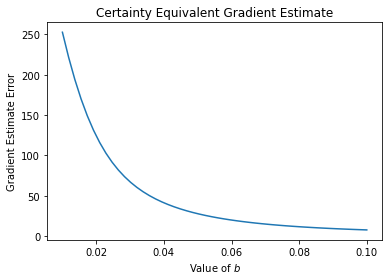
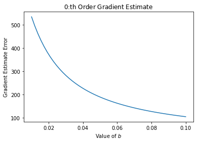
Figure 1: Gradient estimate spread as a function of $b$ for the scalar system (16). Notice that poor controllability (small $b$), leads to noisy gradients. The vertical axes show the standard deviation of $\left\|\nabla_{K}J(K;S)-\widehat{\nabla_{K}J}\right\|_{\mathsf{op}}$ across multiple trajectories.

References

- Silver et al. [2017] David Silver, Julian Schrittwieser, Karen Simonyan, Ioannis Antonoglou, Aja Huang, Arthur Guez, Thomas Hubert, Lucas Baker, Matthew Lai, Adrian Bolton, et al. Mastering the game of go without human knowledge. nature, 550(7676):354–359, 2017.
- Fazel et al. [2018] Maryam Fazel, Rong Ge, Sham Kakade, and Mehran Mesbahi. Global convergence of policy gradient methods for the linear quadratic regulator. In International Conference on Machine Learning, pages 1467–1476. PMLR, 2018.
- Tu and Recht [2019] Stephen Tu and Benjamin Recht. The gap between model-based and model-free methods on the linear quadratic regulator: An asymptotic viewpoint. In Conference on Learning Theory, pages 3036–3083. PMLR, 2019.
- Tsiamis and Pappas [2021] Anastasios Tsiamis and George J Pappas. Linear systems can be hard to learn. arXiv preprint arXiv:2104.01120, 2021.
- Ziemann and Sandberg [2021] Ingvar Ziemann and Henrik Sandberg. On uninformative optimal policies in adaptive lqr with unknown b-matrix. In Learning for Dynamics and Control, pages 213–226. PMLR, 2021.
- Ziemann and Sandberg [2022] Ingvar Ziemann and Henrik Sandberg. Regret lower bounds for learning linear quadratic gaussian systems. arXiv preprint arXiv:2201.01680, 2022.
- Tsiamis et al. [2022] Anastasios Tsiamis, Ingvar Ziemann, Manfred Morari, Nikolai Matni, and George J Pappas. Learning to control linear systems can be hard. arXiv preprint arXiv:2205.14035, 2022.
- Zhang et al. [2020a] Kaiqing Zhang, Alec Koppel, Hao Zhu, and Tamer Basar. Global convergence of policy gradient methods to (almost) locally optimal policies. SIAM Journal on Control and Optimization, 58(6):3586–3612, 2020a.
- Gravell et al. [2019] Benjamin Gravell, Peyman Mohajerin Esfahani, and Tyler Summers. Learning robust control for lqr systems with multiplicative noise via policy gradient. arXiv preprint arXiv:1905.13547, 2019.
- Gravell et al. [2020] Benjamin Gravell, Peyman Mohajerin Esfahani, and Tyler Summers. Learning optimal controllers for linear systems with multiplicative noise via policy gradient. IEEE Transactions on Automatic Control, 66(11):5283–5298, 2020.
- Zhang et al. [2020b] Kaiqing Zhang, Bin Hu, and Tamer Basar. Policy optimization for linear control with robustness guarantee: Implicit regularization and global convergence. In Learning for Dynamics and Control, pages 179–190. PMLR, 2020b.
- Yaghmaie et al. [2022] Farnaz Adib Yaghmaie, Fredrik Gustafsson, and Lennart Ljung. Linear quadratic control using model-free reinforcement learning. IEEE Transactions on Automatic Control, 2022.
- Tang et al. [2021] Yujie Tang, Yang Zheng, and Na Li. Analysis of the optimization landscape of linear quadratic gaussian (lqg) control. In Learning for Dynamics and Control, pages 599–610. PMLR, 2021.
- Mohammadi et al. [2021] Hesameddin Mohammadi, Mahdi Soltanolkotabi, and Mihailo R Jovanović. On the lack of gradient domination for linear quadratic gaussian problems with incomplete state information. In 2021 60th IEEE Conference on Decision and Control (CDC), pages 1120–1124. IEEE, 2021.
- Zheng et al. [2021] Yang Zheng, Luca Furieri, Maryam Kamgarpour, and Na Li. Sample complexity of linear quadratic gaussian (lqg) control for output feedback systems. In Learning for Dynamics and Control, pages 559–570. PMLR, 2021.
- Dean et al. [2020] Sarah Dean, Horia Mania, Nikolai Matni, Benjamin Recht, and Stephen Tu. On the sample complexity of the linear quadratic regulator. Foundations of Computational Mathematics, 20(4):633–679, 2020.
- Preiss et al. [2019] James A Preiss, Sébastien MR Arnold, Chen-Yu Wei, and Marius Kloft. Analyzing the variance of policy gradient estimators for the linear-quadratic regulator. arXiv preprint arXiv:1910.01249, 2019.
- Venkataraman and Seiler [2019] Harish K Venkataraman and Peter J Seiler. Recovering robustness in model-free reinforcement learning. In 2019 American Control Conference (ACC), pages 4210–4216. IEEE, 2019.
- Bernat et al. [2020] Natalie Bernat, Jiexin Chen, Nikolai Matni, and John Doyle. The driver and the engineer: Reinforcement learning and robust control. In 2020 American Control Conference (ACC), pages 3932–3939. IEEE, 2020.
- Boffi et al. [2021] Nicholas M Boffi, Stephen Tu, and Jean-Jacques E Slotine. Regret bounds for adaptive nonlinear control. In Learning for Dynamics and Control, pages 471–483. PMLR, 2021.
- Perdomo et al. [2021] Juan Perdomo, Jack Umenberger, and Max Simchowitz. Stabilizing dynamical systems via policy gradient methods. Advances in Neural Information Processing Systems, 34, 2021.
- Tu et al. [2021] Stephen Tu, Alexander Robey, Tingnan Zhang, and Nikolai Matni. On the sample complexity of stability constrained imitation learning. arXiv preprint arXiv:2102.09161, 2021.
- Ziemann et al. [2022] Ingvar Ziemann, Henrik Sandberg, and Nikolai Matni. Single trajectory nonparametric learning of nonlinear dynamics. arXiv preprint arXiv:2202.08311, 2022.
- Abbasi-Yadkori et al. [2019] Yasin Abbasi-Yadkori, Nevena Lazic, and Csaba Szepesvári. Model-free linear quadratic control via reduction to expert prediction. In The 22nd International Conference on Artificial Intelligence and Statistics, pages 3108–3117. PMLR, 2019.
- Simchowitz and Foster [2020] Max Simchowitz and Dylan Foster. Naive exploration is optimal for online lqr. In International Conference on Machine Learning, pages 8937–8948. PMLR, 2020.
- Cassel and Koren [2021] Asaf B Cassel and Tomer Koren. Online policy gradient for model free learning of linear quadratic regulators with regret. In International Conference on Machine Learning, pages 1304–1313. PMLR, 2021.
- LeCam [1973] Lucien LeCam. Convergence of estimates under dimensionality restrictions. The Annals of Statistics, pages 38–53, 1973.
- Söderström [2002] Torsten Söderström. Discrete-time stochastic systems: estimation and control. Springer Science & Business Media, 2002.
- Doyle [1978] John C Doyle. Guaranteed margins for lqg regulators. IEEE Transactions on automatic Control, 23(4):756–757, 1978.
- Cover [1999] Thomas M Cover. Elements of information theory. John Wiley & Sons, 1999.