Heat conductance oscillations in two weakly connected charge Kondo circuits

Abstract

We revisit a model describing the Seebeck effect on a weak link between two charge Kondo circuits, which has been proposed in the [Phys. Rev. B 97, 085403 (2018)]. We calculate the thermoelectric coefficients in the perturbation theory assuming smallness of the reflection amplitudes of the quantum point contacts. We focus on the linear response equations for the heat conductance in three different scenarios as: Fermi liquid vs Fermi liquid, Fermi liquid vs non-Fermi liquid, non-Fermi liquid vs non-Fermi liquid. The oscillations of the heat conductance as a function of the gate voltage of each quantum dot are analyzed in both Fermi liquid and non-Fermi liquid regimes. We discuss possible experimental realizations of the model to observe the signatures of the non-Fermi liquid behavior in the heat conductance measurements.
Keywords: thermoelectric transport, heat conductance, single/multi-channel charge Kondo effect.
Classification numbers: 73.23.Hk, 73.50.Lw, 72.15.Qm, 73.21.La.

1 INTRODUCTION

Controlling the thermal properties of electronic devices can support technologies based on heat management. A significant amount of work has already been performed to understand heat conduction in nanodevices [1, 2]. It is known that the role of quantum electron transport in many nanostructures affects not only the charge and spin transport phenomena but also the heat transport mechanism. The study of quantum transport, especially the thermoelectric transport in nano-structured devices at very low temperature, is thus an important and rapidly developing topic in recent years. Among a large variety of available nano-devices, quantum dots (QDs) play an important and significant role [3]. On the one hand, QDs are highly controllable and finely adjustable by external fields. On the other hand, QDs being part of the quantum circuits demonstrate pronounced effects of the electron-electron interactions, resonance scattering and quantum interference observable in the quantum transport experiments.

One of the remarkable many-body effects in QD devices is the Kondo effect [4]. A single electron transistor QD device in the Kondo regime shows different universal behaviors at different energies [5]. The conventional single impurity $S=1/2$ single channel Kondo model (1CK) is characterized by a unique energy scale known as the Kondo temperature $T_{K}$ determining the universal behavior of the quantum thermodynamic and transport observables both at $T>T_{K}$ and $T<T_{K}$. The impurity spin of 1CK becomes completely screened by the mobile electrons at $T\to 0$. At energies greater compared to the Kondo temperature $T_{K}$ ($T_{K}$ plays the role of the Fermi energy for 1CK), the system properties can be accessed through the perturbation theory approach. This regime is known as a weak coupling Kondo regime [4, 5]. The behavior of $M$-orbital spin-$S$ Kondo model at the energies lower compared to the Kondo temperature $T_{K}$ depends on the way the mobile electrons screen the impurity spin. For instance, for the full screened case in which $M=2S$ the system at $T<T_{K}$ is in the strong coupling regime, corresponding to the strong coupling fixed point in the renormalization group (RG) flow diagram [5]. This regime is coherent and the system is mentioned having Fermi-liquid (FL) properties. It happens the same when the system is underscreened ($M<2S$). However, for the overscreened case ($M>2S$) which is characterized by intermediate unstable coupling fixed point, the system is potentially having the non-Fermi liquid (NFL) characteristics [5, 6]. Recent studies of the multi-channel Kondo physics in QD devices have focused on the $T<T_{K}$ limit [7, 8, 9, 10, 11, 12, 13, 14, 15]. It is found that it is hard to achieve the strong NFL regime at very low temperature, namely $T\ll T^{*}<T_{K}$, where $T^{*}$ is related to the parameter of the perturbative expansion $|r|$ as $T^{*}=|r|^{2}T_{K}$. The system has a tendency to fall into the FL regime associated with stable FL fixed point [12]. Nevertheless, at higher temperature regimes, $T^{*}<T<T_{K}$, the fingerprints of the weak NFL behavior can be observed [12].

While the conventional Kondo phenomenon is attributed to a spin degree of freedom of the quantum impurity, the unconventional charge Kondo effect deals with an iso-spin implementation of the charge quantization. Recently, the breakthrough experiments [16, 17] have been successful in implementing a setup that consists of a large metallic QD electrically connected to two-dimensional electron gas (2DEG) electrodes through quantum point contacts (QPCs). A strong magnetic field is applied perpendicularly to the 2DEG plane. The 2DEG is in the Integer Quantum Hall (IQH) regime. The QPCs are fine-tuned to satisfy the condition that only one chiral edge current is partially transmitted across the QPCs. The logic behind the mapping of IQH setup to a multi-channel Kondo (MCK) problem has been explained in Refs. [14, 15]. Namely, if we assign the “iso-spin up” to the electrons inside the QD and the “iso-spin down” to the electrons outside the QD, the charge iso-spins flip at QPCs as the backscattering transfers the “moving in-” QD electrons to “moving out-” QD electrons and vice versa. The number of QPCs is equivalent to the number of orbital channels in the conventional $S=1/2$ Kondo problem. Therefore, these experimental setups allow us to investigate the properties of one- or multi-channel Kondo systems characterized by FL or NFL behaviors correspondingly. These experiments mark an important step in the study of the MCK problems. Indeed, fairly recently, another experimental study [18] has successfully implemented a tunable nanoelectronic circuit comprising two coupled hybrid metallic-semiconductor islands, combining the strengths of the two types of materials, which can demonstrate a potential for scalability and a novel quantum critical point.

In the recent years, the thermoelectric transport through QD systems has attracted attentions of both theorists [9, 10, 19, 20] and experimentalists [21, 22, 23, 24]. QDs have advanced applications in thermoelectricity and microelectronics [1, 25, 26] and can be used as the tools for a better understanding of closely correlated systems [27, 28]. Among all the thermoelectric coefficients, the thermopower is the most interesting object due to its high sensitivity to the particle-hole asymmetry of the system. The thermoelectric measurements allow to investigate the effects related to the hole-particle asymmetry and provide information on low-energy excitations in the system [10, 29, 30]. These properties of thermopower open a possibility for capturing the FL – NFL crossover by accessing the NFL mode [12, 14, 30]. Lately, the extended studies [31, 32, 33] have investigated heat conductance in order to better demonstrate the FL and NFL pictures in QD systems. Moreover, understanding thermoelectric properties of a system promotes the study of entropy [34, 35, 36, 37].

In this work, we revisited the setup which has been proposed in 2018 [14]. The generalization of the ideas of Flensberg-Matveev-Furusaki (FMF) theory [7, 8, 9] is adopted to describe the IQH charge Kondo nanodevices [16, 17]. The design for the quantum-dot–quantum-point contact (QD-QPC) devices for investigation of weakly coupled Fermi and non-Fermi liquid states is shown in Fig 1 which can be one of three cases: a) two Fermi liquids; b) a Fermi liquid and a non-Fermi liquid; c) two non-Fermi liquids. We compute perturbatively the thermoelectric coefficients and concentrate on the heat conductance. Discussing the behavior of the heat conductance as a function of temperature and gate voltages in all three cases we find that the FL behavior is more prominent than the NFL one.

The paper is organized as follows. We describe the theoretical model for observing the FL and NFL behavior in Sec. II. General equations for the thermoelectric coefficients are presented in Sec. III. The main results are shown in Sec. IV. We conclude our work in Sec. V.

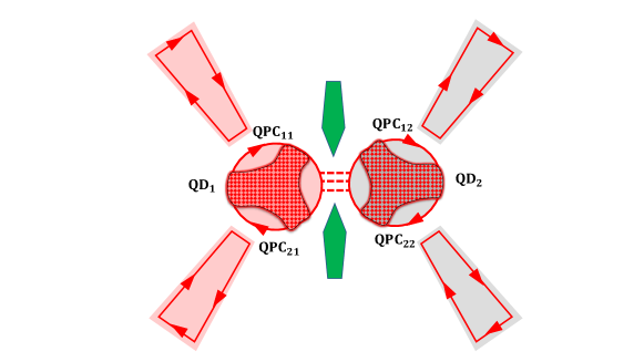
Figure 1: (Color online) Schematic of two charge Kondo site setup. Each site consists of a large metallic quantum dot (QD) (the patch) connected to a two dimensional electron gas (2DEG) (the region inside the circle) and electrode (the trapezoid) through quantum point contacts (QPCs). Controlling the transparencies of the QPCs provides a weak coupling between a) two Fermi liquids; b) a Fermi liquid and a non-Fermi liquid; c) two non-Fermi liquids. Two QDs are connected through the tunnel barrier (red dashed lines) which is controlled by a voltage (the green patches). The pink color stands for the higher temperature $T+\Delta T$ compared to the reference temperature $T$ of the gray color. The currents flowing along the chiral spin edge channel are denoted by red lines with arrows. They are partially transmitted through the almost transparent QPCs.

2 MODEL

We consider a setup (see Fig. 1) consisting of two QD-QPC structures weakly coupled through the tunnel barrier between two QDs. Each large metallic QD with a continuous spectrum is electrically connected to a two-dimensional electron gas (2DEG) denoted by pink and gray areas inside circles and further connected to a large electrode through several QPCs. The 2DEG is in the IQH regime at filling factor $\nu=2$ by applying a strong quantizing magnetic field perpendicularly to it. The QPCs are fine-tuned to achieve a regime where the current flows along the outer spin-polarized edge channel (shown by red color on Fig. 1) is partially transmitted across QPCs. The inner channel (not shown on Fig. 1) is fully reflected and can be ignored. The logic behind the mapping of IQH setup to a single/multichannel Kondo problem has been explained in Refs. [14, 15], so each QD-QPC structure is a single or multi-channel charge Kondo simulator. At the weak link between two QDs, temperature drop happens, namely, the pink color stands for the higher temperature $T+\Delta T$ compared to the reference temperature $T$ of the gray one.

The spinless Hamiltonian describing the two QD-QPC structure coupled weakly at the center (Fig. 1) has the form $H$$=$$H_{1}+H_{T}+H_{2}$, where

$$H_{T}=(td_{1}^{\dagger}d_{2}+\text{h.c.}).$$ (1)

describes the tunneling between two dots, $d_{j}$ is the annihilation operator of an electron in the dot $j,$ ($j=1,2$) at the position of the weak link. Each $\text{QD}_{j}$ is coupled strongly to the leads through $\text{QPC}_{\alpha j}$ ($\alpha=1,2$) so that the whole part [$\text{(QD-QPC)}_{j}$ structure] is described by Hamiltonian $H_{j}$$=$$H_{0j}+H_{Cj}+H_{sj}$. The Hamiltonian $H_{0,j}$ stands for the free part representing two copies of free one-dimensional electrons in $\text{QPC}_{\alpha j}$ ($\alpha j=11,21,12,22$, see Fig. 1) and corresponding patch areas between $\text{QPC}_{\alpha j}$ and $\text{QD}_{j}$ of the $\text{(QD-QPC)}_{j}$:

$$H_{0,j}=\sum_{\alpha=1,2}-iv_{F}\int_{-\infty}^{\infty}dx\left[\psi_{\uparrow,\alpha,j}^{\dagger}\partial_{x}\psi_{\uparrow,\alpha,j}-\psi_{\downarrow,\alpha,j}^{\dagger}\partial_{x}\psi_{\downarrow,\alpha,j}\right].$$ (2)

Here we define $\psi_{\uparrow,\alpha,j}$ ($\psi_{\downarrow,\alpha,j}$) the operator describing one-dimensional fermions which are inside (outside) the $\text{QD}_{j}$ in the $\text{(QD-QPC)}_{j}$, $v_{F}$ is a Fermi velocity. We adopt the units $\hbar=c=k_{B}=1$ in this paper.

The QDs are assumed in the Coulomb blockade regime which is demonstrated by the Hamiltonian $H_{C}$:

$$H_{C,j}=E_{C,j}\left[\hat{n}_{t,j}+\hat{n}_{QPCs,j}-N_{j}(V_{g,j})\right]^{2},$$ (3)

with $E_{C,j}$ is charging energy, $\hat{n}_{t,j}$ and $\hat{n}_{QPCs,j}=\int_{0}^{\infty}\sum_{\alpha}\psi_{\alpha,j}^{\dagger}(x)\psi_{\alpha,j}(x)\,dx$ [38] are the operator of the number of electrons that entered the QD$\!{}_{j}$ through the weak tunnel and the QPCs correspondingly, and $N_{j}$ is a dimensionless parameter which is proportional to the gate voltage $V_{g,j}$. The Hamiltonian $H_{s,j}$ describes the backward scattering at the $\text{QPC}_{\alpha j}$ on the side $j$, which is controlled by a short-range isospin-flip voltage $V_{\alpha j}\left(x\right)$:

$$H_{s,j} =\sum_{\alpha=1,2}\int_{-\infty}^{\infty}dx\left[\psi_{\uparrow,\alpha,j}^{\dagger}\left(x\right)V_{\alpha j}\left(x\right)\psi_{\downarrow,\alpha,j}\left(x\right)e^{-i2k_{F}x}+h.c.\right].$$ (4)

In the spirit of FMF theory [7, 8, 9], we replace $d_{j}^{\dagger}d_{j}=\sum_{\alpha}\psi_{\uparrow,\alpha,j}^{\dagger}(-\infty)\psi_{\uparrow,\alpha,j}(-\infty)F^{\dagger}F$, where $F$ is the operator lowering $\hat{n}_{t,j}$ by unity. The operator $F^{\dagger}(t)$ increases $n_{t,j}$ from $0$ to $1$ at time $t$, while $F(t)$ decreases $n_{t,j}$ back to $0$ from $1$. In the bosonic represention, the fermionic operator is related to the bosonic operator as: $\psi_{(\uparrow/\downarrow),\alpha,j}(x)\sim e^{i\phi_{\alpha,j}(x)}$ with $\phi_{\alpha,j}$ is a bosonization displacement operator describing transport through the $\text{QPC}_{\alpha j}$ of the $\text{(QD-QPC)}_{j}$, with a scatterer at $x$$=$$0$. We can rewrite the $H_{C,j}$ , $H_{0,j}$ and $H_{s,j}$ in the bosonic language as follows.

$$H_{C,j}=E_{C,j}\left[\hat{n_{j}}+\frac{1}{\pi}\sum_{\alpha}\phi_{\alpha,j}(0)-N_{j}(V_{g,j})\right]^{2},$$ (5)

$$H_{0,j}=\sum_{\alpha}\frac{v_{F}}{2\pi}\!\!\!\int_{-\infty}^{\infty}\!\!\!\!\!\!\left\{[\Pi_{\alpha,j}(x)]^{2}+[\partial_{x}\phi_{\alpha,j}(x)]^{2}\right\}dx,$$ (6)

$$H_{s,j}=-\frac{D}{\pi}\sum_{\alpha}|r_{\alpha j}|\cos[2\phi_{\alpha,j}(0)],$$ (7)

where $\Pi_{\alpha,j}$ is the conjugated momentum $[\phi_{\alpha,j}(x),\Pi_{\alpha^{\prime},j}(x^{\prime})]=i\pi\,\delta(x-x^{\prime})\delta_{\alpha\alpha^{\prime}}$, $D$ is a bandwidth, $r_{\alpha j}=-iV_{\alpha j}(2k_{F})/v_{F}$ is the reflection amplitude of the $\text{QPC}_{\alpha j}$.

3 HEAT CURRENT AND HEAT CONDUCTANCE

We sketch the derivation of the electric and heat currents:

$$I_{e} =-2\pi e|t|^{2}\int_{-\infty}^{\infty}d\epsilon\nu_{1}(\epsilon)\nu_{2}(\epsilon)\left[f_{1}(\epsilon)-f_{2}(\epsilon)\right],$$ (8)

$$I_{h} =2\pi|t|^{2}\int_{-\infty}^{\infty}d\epsilon\epsilon\nu_{1}(\epsilon)\nu_{2}(\epsilon)\left[f_{1}(\epsilon)-f_{2}(\epsilon)\right],$$ (9)

with $|t|$ is a modulus of the tunnel matrix element as shown in Eq. (1) and the densities of states are given by equations:

$$\nu_{j}(\epsilon)=-\frac{1}{\pi}\cosh\left(\frac{\epsilon}{2T}\right)\int_{-\infty}^{\infty}G_{j}\left({\displaystyle\frac{1}{2T}+it}\right)e^{i\epsilon t}dt,$$ (10)

where $G_{j}(1/2T+it)$ are exact Green’s Functions (GF) in the terminals $j=1,2$, $f_{1}(\epsilon)=f(\epsilon+e\Delta V/2,T+\Delta T/2)$, $f_{2}(\epsilon)=f(\epsilon-e\Delta V/2,T-\Delta T/2)$ are corresponding Fermi distribution functions, and $df(\epsilon)/d\epsilon=-1/[4T\cosh^{2}(\epsilon/2T)]$, $df(\epsilon)/dT=\epsilon/[4T^{2}\cosh^{2}(\epsilon/2T)]$. The currents in linear response regime are given by

$$I_{e} = 2\pi e^{2}|t|^{2}\frac{\Delta V}{4T}\int_{-\infty}^{\infty}d\epsilon\frac{\nu_{1}(\epsilon)\nu_{2}(\epsilon)}{\cosh^{2}\left({\displaystyle\frac{\epsilon}{2T}}\right)}-2\pi e|t|^{2}\frac{\Delta T}{4T^{2}}\int_{-\infty}^{\infty}d\epsilon\frac{\epsilon\nu_{1}(\epsilon)\nu_{2}(\epsilon)}{\cosh^{2}\left({\displaystyle\frac{\epsilon}{2T}}\right)},$$ (11)

$$I_{h} = -2\pi e|t|^{2}\frac{\Delta V}{4T}\int_{-\infty}^{\infty}d\epsilon\frac{\epsilon\nu_{1}(\epsilon)\nu_{2}(\epsilon)}{\cosh^{2}\left({\displaystyle\frac{\epsilon}{2T}}\right)}+2\pi|t|^{2}\frac{\Delta T}{4T^{2}}\int_{-\infty}^{\infty}d\epsilon\frac{\epsilon^{2}\nu_{1}(\epsilon)\nu_{2}(\epsilon)}{\cosh^{2}\left({\displaystyle\frac{\epsilon}{2T}}\right)}.$$ (12)

Following Onsager’s theory [39], we calculate the thermoelectric coefficients as follows:

$$L_{ee}=\left.T\frac{\partial I}{\partial\Delta V}\right|_{\Delta T=0}=\frac{\pi e^{2}|t|^{2}}{2}\int_{-\infty}^{\infty}d\epsilon\frac{\nu_{1}(\epsilon)\nu_{2}(\epsilon)}{\cosh^{2}\left({\displaystyle\frac{\epsilon}{2T}}\right)},$$ (13)

$$L_{he}=\left.T\frac{\partial I_{h}}{\partial\Delta V}\right|_{\Delta T=0}=-\frac{\pi e|t|^{2}}{2}\int_{-\infty}^{\infty}d\epsilon\frac{\epsilon\nu_{1}(\epsilon)\nu_{2}(\epsilon)}{\cosh^{2}\left({\displaystyle\frac{\epsilon}{2T}}\right)}=L_{eh}=\left.T^{2}\frac{\partial I_{e}}{\partial\Delta T}\right|_{\Delta V=0}\,,$$ (14)

$$L_{hh}=\left.T^{2}\frac{\partial I_{h}}{\partial\Delta T}\right|_{\Delta V=0}=\frac{\pi|t|^{2}}{2}\int_{-\infty}^{\infty}d\epsilon\frac{\epsilon^{2}\nu_{1}(\epsilon)\nu_{2}(\epsilon)}{\cosh^{2}\left({\displaystyle\frac{\epsilon}{2T}}\right)}.$$ (15)

As a result, the heat conductance is defined as

$$G_{H}=\left.\frac{\partial I_{h}}{\partial\Delta T}\right|_{I_{e}=0}=\frac{1}{T^{2}}\left[L_{hh}-\frac{L_{he}^{2}}{L_{ee}}\right].$$ (16)

Plugging in the densities of states in Eq. (10) we get formulas of the thermoelectric coefficients. The last step is to parametrize the exact GF’s at imaginary times as $G_{j}(\tau_{j})$$=$$-\nu_{0j}$$\pi$$T$$\left[\sin\left(\pi T\tau_{j}\right)\right]^{-1}\times$ $K_{j}(\tau_{j})$ with $\nu_{0j}$ is the density of states in the dot computed in the absence of renormalization effects associated with electron-electron interaction . All effects of interaction and scattering are accounted for by the correlator $K_{j}(\tau_{j})=\langle T_{\tau_{j}}\hat{F}_{j}(\tau_{j})\hat{F}_{j}^{\dagger}(0)\rangle$ [9, 10]. It is convenient to introduce a notation $G_{C}=2\pi e^{2}\nu_{01}\nu_{02}|t|^{2}$ for the conductance of the tunnel (central) area between two terminals. Substituting Eq. (10) into Eqs. (11), (12) and performing integration over frequency we obtain after some simplification the general formulas for the thermoelectric coefficients of the two QD-QPC structure nano-device as:

$$L_{ee}=\frac{\pi}{2}G_{C}T^{2}\int_{-\infty}^{\infty}\frac{d\tau}{\cosh^{2}(\pi T\tau)}{\displaystyle K_{1}\left(\frac{1}{2T}+i\tau\right)K_{2}\left(\frac{1}{2T}-i\tau\right),}$$ (17)

$$L_{he}=-\frac{i\pi G_{C}T^{2}}{4e}\int_{-\infty}^{\infty}\frac{d\tau}{\cosh^{2}(\pi T\tau)}\left[\left(\partial_{\tau}K_{1}\left(\frac{1}{2T}+i\tau\right)\right)K_{2}\left(\frac{1}{2T}-i\tau\right)\right.$$

$$-\left.K_{1}\left(\frac{1}{2T}+i\tau\right)\left(\partial_{\tau}K_{2}\left(\frac{1}{2T}-i\tau\right)\right)\right],$$ (18)

$$L_{hh}=\frac{G_{C}}{2e^{2}}\pi T^{2}\int_{-\infty}^{\infty}d\tau\left\{\frac{\pi^{2}T^{2}\left[2-\cosh^{2}(\pi T\tau)\right]}{\cosh^{4}(\pi T\tau)}K_{1}\left({\displaystyle\frac{1}{2T}+i\tau}\right)K_{2}\left({\displaystyle\frac{1}{2T}-i\tau}\right)\right.$$

$$\left.+\frac{1}{\cosh^{2}(\pi T\tau)}\partial_{\tau}K_{1}\left({\displaystyle\frac{1}{2T}+i\tau}\right)\partial_{\tau}K_{2}\left({\displaystyle\frac{1}{2T}-i\tau}\right)\right\}.$$ (19)

The computation of thermoelectric coefficients in Eqs.(17)-(19) essentially needs the explicit form of the electron correlators $K_{j}(1/2T\pm i\tau)$. It depends on the number of conduction channels corresponding to the number of QPCs connecting the QD with the electrode of the site $j$. For our purpose of investigating the physical pictures of the Fermi liquid and non-Fermi liquid states, it is sufficient to consider the single channel and two-channel charge Kondo effects. In the next section we discuss a weak link between a) two Fermi liquids; b) a Fermi liquid and a non-Fermi liquid; c) two non-Fermi liquids in Fig. 1.

4 MAIN RESULTS

Using the above general formulas (17), (18), and (19) to compute the heat conductance as defined in formula (16), we proceed straightforwardly to calculation of the thermoelectric coefficients of the model introduced in Sec. II (see Fig. 1). We label and discuss three important limiting cases one by one in this section. We assume in all calculations that $T\ll\min\left[E_{C,1},E_{C,2}\right]$ [10].

4.1 Fermi liquid – Fermi liquid

This situation happens when each QD is connected to the electrode through a QPC. We assume for illustration purposes that either the $\text{QPC}_{21}$ and $\text{QPC}_{22}$ in Fig.1 are turned off or the differences between the reflection amplitudes of the QPCs in a QD-QPC structure, namely $||r_{11}|-|r_{21}||$ and $||r_{12}|-|r_{22}||$, are big enough [12, 14]. The channel asymmetry plays very important role: the RG controls the flow to the stable FL strong coupling fixed point. We thus have single channel Kondo (1CK) on each side. The correlator $K_{j}\left(\tau\right)$ for spinless case at the first order of the reflection amplitude $|r_{j}|$ of the QPC$\!{}_{j}$ in the perturbative expansion is [10]

$$\!\!K_{j}\left(\tau\right)=\!\left(\frac{\pi^{2}T}{\gamma E_{C,j}}\right)^{2}\!\!\frac{1}{\sin^{2}\left(\pi T\tau\right)}\left[1-2\gamma\xi|r_{j}|\cos\left(2\pi N_{j}\right)+4\pi^{2}\xi\gamma|r_{j}|\frac{T}{E_{C,j}}\sin\left(2\pi N_{j}\right)\cot\left(\pi T\tau\right)\right],$$ (20)

with $\xi=1.59$ is a numerical constant, $\gamma=e^{\bm{C}},\,\bm{C}\approx 0.5772$ is the Euler’s constant [10]. We embed this correlator into Eqs. (17,18,19), we obtain formulas for the thermoelectric coefficients as

$$L_{ee} =A_{1}^{0}G_{C}\frac{T^{5}}{E_{C,1}^{2}E_{C,2}^{2}}\left[1-2\gamma\xi|r_{1}|\cos\left(2\pi N_{1}\right)-2\gamma\xi|r_{2}|\cos\left(2\pi N_{2}\right)\right],$$ (21)

with $A_{1}^{0}=8\pi^{8}/15\gamma^{4}$,

$$L_{he} =-\frac{A_{2}^{0}G_{C}}{e}\frac{T^{7}}{E_{C,1}^{2}E_{C,2}^{2}}\left[\frac{|r_{2}|}{E_{C,2}}\sin\left(2\pi N_{2}\right)+\frac{|r_{1}|}{E_{C,1}}\sin\left(2\pi N_{1}\right)\right],$$ (22)

with $A_{2}^{0}=32\xi\pi^{11}/35\gamma^{3}$, and

$$L_{hh} = \frac{A_{3}^{0}G_{C}}{e^{2}}\frac{T^{7}}{E_{C,1}^{2}E_{C,2}^{2}}\left[1-2\gamma\xi|r_{1}|\cos\left(2\pi N_{1}\right)-2\gamma\xi|r_{2}|\cos\left(2\pi N_{2}\right)\right],$$ (23)

with $A_{3}^{0}=24\pi^{10}/35\gamma^{4}$. So, the heat conductance $G_{H}$ at the lowest order of temperature and reflection amplitudes is

$$G_{H} =\frac{A_{3}^{0}G_{C}}{e^{2}}\frac{T^{5}}{E_{C,1}^{2}E_{C,2}^{2}}\left[1-2\gamma\xi|r_{1}|\cos\left(2\pi N_{1}\right)-2\gamma\xi|r_{2}|\cos\left(2\pi N_{2}\right)\right].$$ (24)

​​​​​​​​

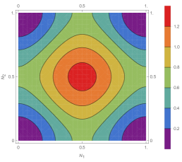
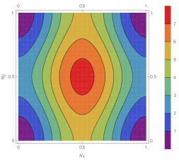
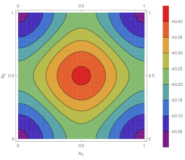
Figure 2: (Color online) Contour plots of the heat conductance $(e^{2}/G_{c})G_{H}\times 10^{6}$ as a function of both dimensionless gate voltages $N_{1}$, $N_{2}$ for the weak link between two Fermi liquid states (left panel), Fermi liquid state – non-Fermi liquid state (central panel), and two non-Fermi liquid states (right panel). Here the reflection amplitudes $|r_{1}|=|r_{2}|=0.088$ and temperature $T=0.01$. We choose $E_{C,1}=E_{C,2}=1$.

The heat conductance as a function of both dimensionless gate voltages $N_{1}$, $N_{2}$ for the weak link between two Fermi liquid states is plotted on Fig. 2 (left panel). We find that the heat conductance in this case oscillates on both gate voltages $N_{1}$ and $N_{2}$ symmetrically. In order to have the heat conductance being positive, the values of the reflection amplitudes and temperature must be much smaller than $E_{C,1},\,E_{C,2}$.

4.2 Fermi liquid – Non-Fermi liquid

This situation happens when the QD in the left side is connected to the electrode through a QPC (either one QPC is off or $||r_{11}|-|r_{21}||$ is big enough, see explanation in the previous subsection) while the QD in the right side is connected to the electrode through two QPCs with the same reflection amplitude $|r_{12}|=|r_{22}|\equiv|r_{2}|$ in Fig. 1. We thus have 1CK on the left side and two-channel Kondo (2CK) on the right side. The correlator $K_{1}\left(\tau_{1}\right)$ for spinless case at the first order of $|r_{1}|$ in the perturbative expansion is shown in Eq. (20), while the correlator $K_{2}\left(\tau_{2}\right)$ for spinful case at the second order of $|r_{2}|$ in the perturbative expansion is [10]

$$K_{2}\left(\tau_{2}\right) = \frac{\pi^{2}T}{2\gamma E_{C,2}}\frac{1}{|\sin\left(\pi T\tau_{2}\right)|}\left[1+\frac{2\gamma E_{C2}}{\pi^{4}T}|r_{2}|^{2}\left[\cos\left(2\pi N_{2}\right)+1\right]F\left(\tau_{2}\right)\right.$$ (25)

$$\left.-\frac{8\gamma}{\pi^{2}}|r_{2}|^{2}\sin\left(2\pi N_{2}\right)\ln\left[\frac{E_{C,2}}{T}\right]\ln\tan\left(\frac{\pi T\tau_{2}}{2}\right)\right],$$

with $F\left(\tau\right)$ expressed in terms of dilogarithm function ${\rm Li}_{2}(x)=-\int_{0}^{x}t^{-1}\ln(1-t)dt$ [40] as

$$F\left(\tau\right) = i\left\{3\left[-i\pi T\tau\ln\tan\left(\frac{\pi T\tau}{2}\right)-\text{Li}_{2}\left[-i\tan\left(\frac{\pi T\tau}{2}\right)\right]+\text{Li}_{2}\left[i\tan\left(\frac{\pi T\tau}{2}\right)\right]\right]\right.$$ (26)

$$\left.+i\pi\left(1+T\tau\right)\ln\cot\left(\frac{\pi T\tau}{2}\right)-\text{Li}_{2}\left[-i\cot\left(\frac{\pi T\tau}{2}\right)\right]+\text{Li}_{2}\left[i\cot\left(\frac{\pi T\tau}{2}\right)\right]\right\}.$$

Embedding these correlation functions into Eqs. (17)-(19), we obtain

$$L_{ee}=C_{1}^{0}G_{C}\frac{T^{4}}{E_{C,1}^{2}E_{C,2}}\left[1-2\gamma\xi|r_{1}|\cos\left(2\pi N_{1}\right)-{\color[rgb]{0,0,0}C_{1}^{1}|r_{2}|^{2}\frac{E_{C,2}}{T}\cos^{2}\left(\pi N_{2}\right)}\right],$$ (27)

with $C_{1}^{0}=3\pi^{7}/32\gamma^{3}$ and $C_{1}^{1}=\left(189\zeta\text{$\left(3\right)$}-62\right)16\gamma/27\pi^{5}$, $\zeta(s)=\sum_{n=1}^{\infty}n^{-s}$ is the Riemann $\zeta$-function, $\zeta\text{$\left(3\right)$}\approx 1.2$ is Apery’s constant.

$$L_{he} =-\frac{C_{2}^{0}G_{C}}{e}\frac{T^{5}}{E_{C,1}^{2}E_{C,2}}\left[|r_{1}|\frac{T}{E_{C,1}}\sin\left(2\pi N_{1}\right)+{\color[rgb]{0,0,0}C_{2}^{1}|r_{2}|^{2}\ln\left[\frac{E_{C,2}}{T}\right]\sin\left(2\pi N_{2}\right)}\right],$$ (28)

with $C_{2}^{0}=\pi^{10}\xi/8\gamma^{2}$ and $C_{2}^{1}=256/25\pi^{5}\xi$,

$$L_{hh}=\frac{C_{3}^{0}G_{C}}{e^{2}}\frac{T^{6}}{E_{C,1}^{2}E_{C,2}}\left[1-2\gamma\xi|r_{1}|\cos\left(2\pi N_{1}\right)-{\color[rgb]{0,0,0}C_{3}^{1}|r_{2}|^{2}\frac{E_{C,2}}{T}\cos^{2}\!\left(\pi N_{2}\right)}\right]$$ (29)

with $C_{3}^{0}=3\pi^{9}/32\gamma^{3}$ and $C_{3}^{1}=\left(189\zeta\text{$\left(3\right)$}-62\right)16\gamma/27\pi^{5}$. So, the heat conductance is

$$G_{H}=\!\frac{C_{3}^{0}G_{C}}{e^{2}}\frac{T^{4}}{E_{C,1}^{2}E_{C,2}}\!\!\left[\!\!1-2\gamma\xi|r_{1}|\!\cos\left(2\pi N_{1}\!\right)-{\color[rgb]{0,0,0}C_{3}^{1}|r_{2}|^{2}\frac{E_{C,2}}{T}\!\cos^{2}\!\left(\pi N_{2}\!\right)-\frac{\left(C_{2}^{0}\right)^{2}}{C_{3}^{0}C_{1}^{0}}|r_{1}|^{2}\frac{T^{2}}{E_{C,1}^{2}}\!\sin^{2}\!\left(2\pi N_{1}\!\right)}\!\right]$$ (30)

The heat conductance oscillates on the gate voltages $N_{1}$, $N_{2}$ asymmetrically when the Fermi liquid state and non-Fermi liquid state are weakly coupled as shown in Fig. 2 (central panel). The heat conductance depends on $N_{2}$ [as $|r_{2}|^{2}T^{3}\cos^{2}\left(\pi N_{2}\right)$] less strong than on $N_{1}$ [as $|r_{1}|T^{4}\cos\left(2\pi N_{1}\right)$ and $|r_{1}|^{2}T^{6}\sin^{2}\left(2\pi N_{1}\right)$]. Thus, it is easy to find that the FL-1CK dominates in the heat conductance. One may think that the reason is the flow of the heat energy from the FL-1CK side to the NFL-2CK one but it is not the case. Even though the NFL-2CK site is at higher temperature, the FL-1CK still contributes from the first order term. In order to have effects of NFL-2CK considerable in Eq. (30), the reflection amplitude $|r_{2}|$ and temperature must satisfy $T^{-3/2}|r_{2}|/|r_{1}|\geq 49.3718$ and $\left(|r_{2}|^{2}/|r_{1}|\right)/T\geq 9.94$. In fact, these conditions can be satisfied in experiments, we predict that there exists a temperature $T^{*}$ at which the crossover FL – NFL happens in the heat conductance [14, 30].

4.3 Non-Fermi liquid – Non-Fermi liquid

This regime is realized when both QD in both sides are connected to the electrode through two QPCs with the same reflection amplitude $|r_{j}|$, see Fig. 1. We thus have 2CK on each side. We embed the correlator $K_{j}\left(\tau_{j}\right)$ for spinful case at the second order of $|r_{j}|$ in the perturbative expansion as in Eq. (25) [10] into Eqs. (17,18,19), we obtain

$$L_{ee}=P_{1}^{0}G_{C}\frac{T^{3}}{E_{C,1}E_{C,2}}\left[1-{\color[rgb]{0,0,0}P_{1}^{1}\sum_{j=1,2}|r_{j}|^{2}\frac{E_{C,j}}{T}\cos^{2}\left(\pi N_{j}\right)}\right],$$ (31)

with $P_{1}^{0}=\pi^{4}/6\gamma^{2}$, $P_{1}^{1}=\left(16\ln 2-1\right)\gamma/\pi^{3}$,

$$L_{he}=-\frac{P_{2}^{0}G_{C}}{e}\frac{T^{4}}{E_{C,1}E_{C,2}}\sum_{j=1,2}|r_{j}|^{2}\ln\left[\frac{E_{C,j}}{T}\right]\sin\left(2\pi N_{j}\right),$$ (32)

with $P_{2}^{0}=3\pi^{4}/16\gamma$,

$$L_{hh} = \frac{P_{3}^{0}G_{C}}{e^{2}}\frac{T^{5}}{E_{C,1}E_{C,2}}\left[1-{\color[rgb]{0,0,0}P_{3}^{1}\sum_{j=1,2}|r_{j}|^{2}\frac{E_{C,j}}{T}\cos^{2}\left(\pi N_{j}\right)}\right],$$ (33)

with $P_{3}^{0}=2\pi^{6}/15\gamma^{2}$, $P_{3}^{1}=\left(16\ln 2-49/64\right)\gamma/\pi^{3}$. So, the heat conductance at the lowest order which depends on the gate voltage $N_{j}$ is:

$$G_{H} = \frac{P_{3}^{0}G_{C}}{e^{2}}\frac{T^{3}}{E_{C,1}E_{C,2}}\left[1-{\color[rgb]{0,0,0}P_{3}^{1}\sum_{j=1,2}|r_{j}|^{2}\frac{E_{C,j}}{T}\cos^{2}\left(\pi N_{j}\right)}\right].$$ (34)

We find that in Eq. (34), following the zero order in the perturbative series is the second order of the reflection amplitudes. It means the heat conductance oscillates weakly on the gate voltage $N_{j}$. The heat conductance as a function of both dimensionless gate voltages $N_{1}$, $N_{2}$ is plotted for the weak link between two non-Fermi liquid states on Fig. 2 (right panel).

The Eqs. (24), (30), and (34) are central results of this paper. The heat conductance is affected by FL states more strongly than by NFL states. The zero order terms (the main terms) follow the temperature scaling $T^{5}$, $T^{4}$, and $T^{3}$ corresponding to the situations coupling between two FL states, between FL and NFL states, and between two NFL states. The Coulomb oscillations appear at the first order term when one or both of the charge Kondo circuits is/are in FL regime while they appear at the second order when one or both sides is/are in NFL states. It is understood that the NFL states originated from a two-channel charge Kondo with strong fluctuations of the isospin. Therefore, at the lowest order, the heat conductance is deducted by a percentage which is proportional to $1/T$ (see terms inside the bracket) concerning NFL states.

5 CONCLUSION

In summary, we have derived equations for the heat conductance of a quantum circuit containing a weak coupling between two QD-QPC structures where each one is corresponding to a charge Kondo simulator: either single channel – Fermi liquid state or two channel – non-Fermi liquid state. The heat conductance is computed in perturbation theory assuming the smallness of the reflection amplitudes at the QPCs. In this regime the heat conductance in the complex charge Kondo circuit is small and consistent with classical explanation for bulk materials [41]. The gate voltage dependence is more pronounced when the Kondo states are FL than when the Kondo states are NFL. For the mixed regime when the weak link connects the FL and NFL states, the FL state dominates in the heat conductance. All regimes can be experimentally verified in quantum transport measurements with charge Kondo simulators.

Other interesting directions for future work can be investigating heat conduction in the presence of Kondo charge correlation in different complex setups. The extensions of the calculations beyond the linear response [42] and/or the perturbation theory is a challenging problem [43]. Investigations of the effects of the strong couplings between quantum dots in the Kondo regime are currently open for future research [18, 43].

References

- [1] V. Zlatic and R. Monnier, Modern Theory of Thermoelectricity, Oxford University Press, 2014.
- [2] G. Benenti, G. Casati, K. Saito, and R. Whitney, Phys. Rep. 694 (2017) 1.
- [3] Y. M. Blanter and Y. V. Nazarov, Quantum Transport: Introduction to Nanoscience, Cambridge University Press, Cambridge, 2009.
- [4] J. Kondo, Prog. Theor. Phys. 32 (1964) 37.
- [5] A.C. Hewson, The Kondo Problem to Heavy Fermions, Cambridge Studies in Magnetism, Cambridge University Press, Cambridge, 1993.
- [6] P. Nozieres and A. Blandin, J. Phys. 41 (1980) 193.
- [7] K. Flensberg, Phys. Rev. B 48 (1993) 11156.
- [8] K. A. Matveev, Phys. Rev. B 51 (1995) 1743.
- [9] A. Furusaki, K. A. Matveev, Phys. Rev. B 52 (1995) 16676.
- [10] A. V. Andreev, K. A. Matveev, Phys. Rev. Lett. 86 (2001) 280; Phys. Rev. B 66 (2002) 045301.
- [11] K. Le Hur and G. Seelig, Phys. Rev. B 65 (2002) 165338.
- [12] T. K. T. Nguyen, M. N. Kiselev, and V. E. Kravtsov, Phys. Rev. B 82 (2010) 113306.
- [13] T.K.T. Nguyen and M.N. Kiselev, Phys. Rev. B 92 (2015) 045125.
- [14] T. K. T. Nguyen, M. N. Kiselev, Phys. Rev. B 97 (2018) 085403.
- [15] T. K. T. Nguyen, M. N. Kiselev, Phys. Rev. Lett. 125 (2020) 026801.
- [16] Z. Iftikhar, S. Jezouin, A. Anthore, U. Gennser, F. D. Parmentier, A. Cavanna and F. Pierre, Nature 526 (2015) 233.
- [17] Z. Iftikhar, A. Anthore, A. K. Mitchell, F. D. Parmentier, U. Gennser, A. Ouerghi, A. Cavanna, C. Mora, P. Simon, and F. Pierre, Science 360 (2018) 1315.
- [18] W. Pouse, L. Peeters, C. L. Hsueh, U. Gennser, A. Cavanna, M. A. Kastner, A. K. Mitchell, D. Goldhaber-Gordon, arXiv:2108.12691.
- [19] C. W. J. Beenakker and A. A. M. Staring, Phys. Rev. B 46 (1992) 9667.
- [20] M. Turek and K. A. Matveev, Phys. Rev. B 65 (2002) 115332.
- [21] A. A. M. Staring, L. W. Molenkamp, B. W. Alphenaar, H. van Houten, O. J. A. Buyk, M. A. A. Mabesoone, C. W. J. Beenakker, and C. T. Foxon, Europhys. Lett. 22 (1993) 57.
- [22] A. S. Dzurak, C. G. Smith, C. H. W. Barnes, M. Pepper, L. Martin-Moreno, C. T. Liang, D. A. Ritchie, and G. A. C. Jones, Phys. Rev. B 55 (1997) R10197(R).
- [23] R. Scheibner, H. Buhmann, D. Reuter, M. N. Kiselev, and L. W. Molenkamp, Phys. Rev. Lett. 95 (2005) 176602.
- [24] R. M. Potok, I. G. Rau, H. Shtrikman, Y. Oreg, and D. Goldhaber-Gordon, Nature (London) 446 (2007) 167.
- [25] M. S. Dresselhaus, G. Dresselhaus, X. Sun, Z. Zhang, S. B. Cronin, and T. Koga, Phys. Solid State 41 (1999) 679.
- [26] G. Benenti, G. Casati, K. Saito, and R. S. Whitney, Phys. Rep. 694 (2017) 1.
- [27] V. Zlatic, T. A. Costi, A. C. Hewson, and B. R. Coles, Phys. Rev. B 48 (1993) 16152.
- [28] T.-S. Kim and S. Hershfield, Phys. Rev. B 67 (2003) 165313.
- [29] M. G. Vavilov and A. D. Stone, Phys. Rev. B 72 (2005) 205107.
- [30] D. B. Karki and M. N. Kiselev, Phys. Rev. B 100 (2019) 125426.
- [31] D. B. Karki, Phys. Rev. B 102 (2020) 245430.
- [32] D. B. Karki, Phys. Rev. B 102 (2020) 115423.
- [33] A. I. Pavlov and M. N. Kiselev, Phys. Rev. B 103 (2021) L201107.
- [34] K. Yang and B. I. Halperin, Phys. Rev. B 79 (2009) 115317.
- [35] W. E. Chickering, J. P. Eisenstein, L. N. Pfeiffer, and K. W. West, Phys. Rev. B 87 (2013) 075302.
- [36] C.-Y. Hou, K. Shtengel, G. Refael, and P. M. Goldbart, New J. Phys. 14 (2012) 105005.
- [37] Y. Kleeorin, H. Thierschmann, H. Buhmann, A. Georges, L. W. Molenkamp, and Y. Meir, Nat. Commun. 10 (2019) 5801.
- [38] I. L. Aleiner and L. I. Glazman, Phys. Rev. B 57 (1998) 9608.
- [39] L. Onsager, Phys. Rev. 37, 405 (1931); L. Onsager, Phys. Rev. 38 (1931) 2265.
- [40] M. Abramowitz and I. A. Stegun, ‘’Handbook of Mathematical Functions: With Formulas, Graphs, and Mathematical Tables”, In: M. Abramowitz and I. A. Stegun, Eds., Dover Books on Advanced Mathematics, Dover Publications, New York, 1965.
- [41] D. W. Hahn and M. N. Ozisik, Heat Conduction, 3rd Edition , Wiley Publisher, Hoboken, New Jersey, 2012.
- [42] D. B. Karki and M. N. Kiselev, Phys. Rev. B 96 (2017) 121403(R).
- [43] D. B. Karki, E. Boulat, and C. Mora, arXiv:2204.08549.