varFEM: variational formulation based programming for finite element methods in Matlab

Abstract

This paper summarizes the development of varFEM, which provides a realization of the programming style in FreeFEM by using the Matlab language.

1 Introduction

FreeFEM is a popular 2D and 3D partial differential equations (PDE) solver based on finite element methods (FEMs) [2], which has been used by thousands of researchers across the world. The highlight is that the programming language is consistent with the variational formulation of the underlying PDEs, referred to as the variational formulation based programming in this article. We intend to develop an FEM package in a similar way of FreeFEM using the language of Matlab, named varFEM. The similarity here only refers to the programming style of the main or test script, not to the internal architecture of the software.

This programming paradigm is usually organized in an object-oriented language, which makes it difficult for readers or users to understand and modify the code, and further redevelop the package (although it is a good way to develop softwares). Upon rethinking the process of finite element programming, it becomes clear that the assembly of the stiffness matrix and load vector essentially reduces to the numerical integration of some typical bilinear and linear forms with respect to basis functions. In this regard, the package $i$FEM, written in Matlab, has provided robust, efficient, and easy-following codes for many mathematical and physical problems in both two and three dimensions [1]. On this basis, we successfully developed the variational formulation based programming for the conforming $\mathbb{P}_{k}$-Lagrange ($k\leq 3$) FEMs in two dimensions by utilizing the Matlab language. The underlying idea can be generalized to other types of finite elements for both two- and three-dimensional problems on unstructured simplicial meshes. The package is accessible on https://github.com/Terenceyuyue/varFEM (see the varFEM folder).

The article is organized as follows. In Section 2, we introduce the basic idea in varFEM through a model problem. In Section 3, we demonstrate the use of varFEM for several typical examples, including a complete implementation of the model problem, the vector finite element for the linear elasticity, the mixed FEMs for bihamonic equation and Stokes problem, and the iterative scheme for the heat equation. We also demonstrate the ability of varFEM to solve complex problems in Section 4.

2 Variational formulation based programming in varFEM

We introduce the variational formulation based programming in varFEM via a model problem, so as to facilitate the underlying design idea.

2.1 Programming for a model problem

Let $\Omega=(0,1)^{2}$ and consider the second-order elliptic problem:

$$\begin{cases}-\nabla\cdot(a\nabla u)+cu=f\quad&\text{in}~{}~{}\Omega,\\ u=g_{D}\quad&\text{on}~{}~{}\Gamma_{D},\\ g_{R}u+a\partial_{n}u=g_{N}\quad&\text{on}~{}~{}\Gamma_{R},\end{cases}$$ (2.1)

where $\Gamma_{D}$ and $\Gamma_{R}=\partial\Omega\backslash\Gamma_{D}$ are the Dirichlet boundary and Robin boundary, respectively. For brevity, we refer to $g_{R}$ as the Robin boundary data function and $g_{N}$ as the Neumann boundary data function. For homogenous Dirichlet boundary condition, the variational problem is to find $u\in V:=H_{0}^{1}(\Omega)$ such that

$$a(v,u)=\ell(v),\quad v\in V,$$

where

$$a(v,u)=\int_{\Omega}{a\nabla v\cdot\nabla u}{\rm d}\sigma+\int_{\Omega}{cvu}{\rm d}\sigma+\int_{\Gamma_{R}}g_{R}vu{\rm d}s,$$

$$\ell(v)=\int_{\Omega}fv{\rm d}\sigma+\int_{\Gamma_{R}}g_{N}v{\rm d}s.$$

Here, the test function is placed in the first entry of $a(\cdot,\cdot)$ since

$$a(v,u)=\bm{v}^{T}\bm{Au},\quad\bm{A}=(a(\varphi_{i},\phi_{j}))_{m\times n},$$

where $\bm{v}=(v_{1},\cdots,v_{m})^{T}$ and $\bm{u}=(u_{1},\cdots,u_{n})^{T}$, with

$$v=\sum\limits_{i=1}^{m}v_{i}\varphi_{i},\quad u=\sum\limits_{i=1}^{n}u_{i}\phi_{i}.$$

2.1.1 The assembly of bilinear forms

The first step is to obtain the stiffness matrix associated with the bilinear form

$$\int_{\Omega}a\nabla v\cdot\nabla u{\rm d}\sigma+\int_{\Omega}cvu{\rm d}\sigma$$

on the approximated domain, where for simplicity we have used the original notation $\Omega$ to represent a triangular mesh. The computation in varFEM reads

⬇

1% Omega

2Coef = {a, c};

3Test = {'v.grad', 'v.val'};

4Trial = {'u.grad', 'u.val'};

5kk = int2d(Th,Coef,Test,Trial,Vh,quadOrder);

Here, Th represents the triangular mesh, which provides some necessary auxiliary data structures. We set up the triple (Coef,Test,Trial), for the coefficients, test functions and trial functions in variational form, respectively. It is obvious that v.grad is for $\nabla v$ and v.val is for $v$ itself. The routine int2d.m computes the stiffness matrix corresponding to the bilinear form on the two-dimensional region, i.e.

$$A=(a_{ij}),\quad a_{ij}=a(\Phi_{i},\Phi_{j}),$$

where $\Phi_{i}$ are the global shape functions of the finite element space Vh. The integral of the bilinear form, as $(\nabla\Phi_{i},\nabla\Phi_{j})_{\Omega}$, will be approximated by using the Gaussian quadrature formula with quadOrder being the order of accuracy.

The second step is to compute the stiffness matrix for the bilinear form on the Robin boundary $\Gamma_{R}$:

$$\int_{\Gamma_{R}}g_{R}vu{\rm d}s.$$

The code can be written as follows.

⬇

1% Gamma_R

2Th.elem1d = Th.bdEdgeType{1};

3Th.elem1dIdx = Th.bdEdgeIdxType{1};

4Coef = {g_R};

5Test = {'v.val'};

6Trial = {'u.val'};

7kk = kk + int1d(Th,Coef,Test,Trial,Vh,quadOrder);

Here, int1d.m gives the contribution to the stiffness matrix on the one-dimensional boundary edges of the mesh. Note that we must provide the connectivity list elem1d of the boundary edges of $\Gamma_{R}$ and the associated indices elem1dIdx in the data structure edge introduced later.

2.1.2 The assembly of linear forms

For the linear forms, we first consider the integral for the source term:

$$\int_{\Omega}fv{\rm d}\sigma.$$

The load vector can be assembled as

⬇

1% Omega

2Coef = pde.f; Test = 'v.val';

3ff = int2d(Th,Coef,Test,[],Vh,quadOrder);

We set Trial = [] to indicate the linear form.

The computation of the load vector associated with the Neumann boundary data function $g_{N}$, i.e.,

$$\int_{\Gamma_{R}}g_{N}v{\rm d}s$$

reads

⬇

1% Gamma_R

2Coef = g_N; Test = 'v.val';

3ff = ff + int1d(Th,Coef,Test,[],Vh,quadOrder);

2.2 Data structures for triangular meshes

We adopt the data structures given in $i$FEM [1]. All related data are stored in the Matlab structure Th, which is computed by using the subroutine FeMesh2d.m as

⬇

1Th = FeMesh2d(node,elem,bdStr);

The triangular meshes are represented by two basic data structures node and elem, where node is an ${\leavevmode\lstinline{{\lst@@@set@language\lst@@@set@numbers\lst@@@set@frame\lst@@@set@rulecolor\lst@@@set@language\lst@@@set@numbers\lst@@@set@frame\lst@@@set@rulecolor\lst@@@set@language\lst@@@set@numbers\lst@@@set@frame\footnotesize\small{\@listingGroup{ltx_lst_identifier}{N}}}}}\times 2$ matrix with the first and second columns contain $x$- and $y$-coordinates of the nodes in the mesh, and elem is an ${\leavevmode\lstinline{{\lst@@@set@language\lst@@@set@numbers\lst@@@set@frame\lst@@@set@rulecolor\lst@@@set@language\lst@@@set@numbers\lst@@@set@frame\lst@@@set@rulecolor\lst@@@set@language\lst@@@set@numbers\lst@@@set@frame\footnotesize\small{\@listingGroup{ltx_lst_identifier}{NT}}}}}\times 3$ matrix recording the vertex indices of each element in a counterclockwise order, where N and NT are the numbers of the vertices and triangular elements.

In the current version, we only consider the $\mathbb{P}_{k}$-Lagrange finite element spaces with $k$ up to 3. In this case, there are two important data structures edge and elem2edge. In the matrix edge(1:NE,1:2), the first and second rows contain indices of the starting and ending points. The column is sorted in the way that for the $k$-th edge, edge(k,1)<edge(k,2) for ${k=1,2,\cdots,\leavevmode\lstinline{{\lst@@@set@language\lst@@@set@numbers\lst@@@set@frame\lst@@@set@rulecolor\lst@@@set@language\lst@@@set@numbers\lst@@@set@frame\lst@@@set@rulecolor\lst@@@set@language\lst@@@set@numbers\lst@@@set@frame\footnotesize\small{\@listingGroup{ltx_lst_identifier}{NE}}}}}$. The matrix elem2edge establishes the map of local index of edges in each triangle to its global index in matrix edge. By convention, we label three edges of a triangle such that the $i$-th edge is opposite to the $i$-th vertex. We refer the reader to https://www.math.uci.edu/~chenlong/ifemdoc/mesh/auxstructuredoc.html for some detailed information.

To deal with boundary integrals, we first exact the boundary edges from edge and store them in matrix bdEdge. In the input of FeMesh2d, the string bdStr is used to indicate the interested boundary part in bdEdge. For example, for the unit square $\Omega=(0,1)^{2}$,

• bdStr = 'x==1' divides bdEdge into two parts: bdEdgeType{1} gives the boundary edges on $x=1$, and bdEdgeType{2} stores the remaining part.

• bdStr = {'x==1','y==0'} separates the boundary data bdEdge into three parts: bdEdgeType{1} and bdEdgeType{2} give the boundary edges on $x=1$ and $y=0$, respectively, and bdEdgeType{3} stores the remaining part.

• bdStr = [] implies that bdEdgeType{1} = bdEdge.

We also use bdEdgeIdxType to record the index in matrix edge, and bdNodeIdxType to store the nodes for respective boundary parts. Note that we determine the boundary of interest by the coordinates of the midpoint of the edge, so 'x==1' can also be replaced by a statement like 'x>0.99'.

2.3 Code design of int2d.m and assem2d.m

In this article we only discuss the implementation of the bilinear forms in two dimensions.

2.3.1 The scalar case: assem2d.m

In this subsection we introduce the details of writing the subroutine assem2d.m to assemble a two-dimensional scalar bilinear form

$$a(v,u),\quad v=\varphi_{i},~{}~{}u=\phi_{j},\quad i=1,\cdots,m,~{}~{}j=1,\cdots,n,$$

where the test function $v$ and the trial function $u$ are allowed to match different finite element spaces, which can be found in mixed finite element methods for Stokes problems. For the scalar case, assem2d.m is essentially the same as int2d.m, while the later one can be used to deal with vector cases like linear elasticity problems. To handle different spaces, we write Vh = {'P1', 'P2' } for the input of assem2d.m, where Vh{1} is for $v$ and Vh{2} is for $u$. For simplicity, it is also allowed to write Vh = 'P1' when $v$ and $u$ are in the same space.

Let us discuss the case where $v$ and $u$ lie in the same space. Suppose that the bilinear form contains only first-order derivatives. Then the possible combinations are

$$\int_{K}{avu}{\rm d}x,\quad\int_{K}av_{x}u{\rm d}x,\quad\int_{K}av_{y}u{\rm d}\sigma,$$

$$\int_{K}avu_{x}{\rm d}\sigma,\quad\int_{K}av_{x}u_{x}{\rm d}\sigma,\quad\int_{K}av_{y}u_{x}{\rm d}\sigma,$$

$$\int_{K}avu_{y}{\rm d}\sigma,\quad\int_{K}av_{x}u_{y}{\rm d}\sigma,\quad\int_{K}av_{y}u_{y}{\rm d}\sigma.$$

Of course, we often encounter the gradient form

$$\int_{K}a\nabla v\cdot\nabla u{\rm d}\sigma=\int_{K}a(v_{x}u_{x}+v_{y}u_{y}){\rm d}\sigma.$$

We take the second bilinear form as an example. Let

$$a_{K}(v,u)=\int_{K}av_{x}u{\rm d}\sigma,$$

and consider the $\mathbb{P}_{1}$-Lagrange finite element. Denote the local basis functions to be $\phi_{1},\phi_{2},\phi_{3}$. Then the local stiffness matrix is

$$A_{K}=\int_{K}a\begin{bmatrix}\partial_{x}\phi_{1}\\ \partial_{x}\phi_{2}\\ \partial_{x}\phi_{3}\end{bmatrix}\begin{bmatrix}\phi_{1}&\phi_{2}&\phi_{3}\end{bmatrix}{\rm d}\sigma.$$

Let

$$v_{1}=\partial_{x}\phi_{1},~{}~{}v_{2}=\partial_{x}\phi_{2},~{}~{}v_{3}=\partial_{x}\phi_{3};\quad u_{1}=\phi_{1},~{}~{}u_{2}=\phi_{2},~{}~{}u_{3}=\phi_{3}.$$

Then

$$A_{K}=(k_{ij})_{3\times 3},\quad k_{ij}=\int_{K}av_{i}u_{j}{\rm d}\sigma.$$

The integral will be approximated by the Gaussian quadrature rule:

$$k_{ij}=\int_{K}av_{i}u_{j}{\rm d}\sigma=|K|\sum\limits_{p=1}^{n_{g}}w_{p}a(x_{p},y_{p})v_{i}(x_{p},y_{p})u_{j}(x_{p},y_{p}),$$

where $(x_{p},y_{p})$ is the $p$-th quadrature point. In the implementation, we in advance store the quadrature weights and the values of basis functions or their derivatives in the following form:

$${{w_{p},\qquad\leavevmode\lstinline{{\lst@@@set@language\lst@@@set@numbers\lst@@@set@frame\lst@@@set@rulecolor\lst@@@set@language\lst@@@set@numbers\lst@@@set@frame\lst@@@set@rulecolor\lst@@@set@language\lst@@@set@numbers\lst@@@set@frame\footnotesize\small{\@listingGroup{ltx_lst_identifier}{vi}}}}}(:,p)=\begin{bmatrix}v_{i}|_{(x_{p}^{1},y_{p}^{1})}\\ v_{i}|_{(x_{p}^{2},y_{p}^{2})}\\ \vdots\\ v_{i}|_{(x_{p}^{\text{NT}},y_{p}^{\text{NT}})}\end{bmatrix},\qquad\leavevmode\lstinline{{\lst@@@set@language\lst@@@set@numbers\lst@@@set@frame\lst@@@set@rulecolor\lst@@@set@language\lst@@@set@numbers\lst@@@set@frame\lst@@@set@rulecolor\lst@@@set@language\lst@@@set@numbers\lst@@@set@frame\footnotesize\small{\@listingGroup{ltx_lst_identifier}{uj}}}}}(:,p)=\begin{bmatrix}u_{j}|_{(x_{p}^{1},y_{p}^{1})}\\ u_{j}|_{(x_{p}^{2},y_{p}^{2})}\\ \vdots\\ u_{j}|_{(x_{p}^{\text{NT}},y_{p}^{\text{NT}})}\end{bmatrix},\qquad p=1,\cdots,n_{g},$$

where vi associated with $v_{i}$ is of size ${{\leavevmode\lstinline{{\lst@@@set@language\lst@@@set@numbers\lst@@@set@frame\lst@@@set@rulecolor\lst@@@set@language\lst@@@set@numbers\lst@@@set@frame\lst@@@set@rulecolor\lst@@@set@language\lst@@@set@numbers\lst@@@set@frame\footnotesize\small{\@listingGroup{ltx_lst_identifier}{NT}}}}}\times\leavevmode\lstinline{{\lst@@@set@language\lst@@@set@numbers\lst@@@set@frame\lst@@@set@rulecolor\lst@@@set@language\lst@@@set@numbers\lst@@@set@frame\lst@@@set@rulecolor\lst@@@set@language\lst@@@set@numbers\lst@@@set@frame\footnotesize\small{\@listingGroup{ltx_lst_identifier}{ng}}}}}$ with the $p$-th column given by ${\leavevmode\lstinline{{\lst@@@set@language\lst@@@set@numbers\lst@@@set@frame\lst@@@set@rulecolor\lst@@@set@language\lst@@@set@numbers\lst@@@set@frame\lst@@@set@rulecolor\lst@@@set@language\lst@@@set@numbers\lst@@@set@frame\footnotesize\small{\@listingGroup{ltx_lst_identifier}{vi}}}}}(:,p)$. Let ${\leavevmode\lstinline{{\lst@@@set@language\lst@@@set@numbers\lst@@@set@frame\lst@@@set@rulecolor\lst@@@set@language\lst@@@set@numbers\lst@@@set@frame\lst@@@set@rulecolor\lst@@@set@language\lst@@@set@numbers\lst@@@set@frame\footnotesize\small{\@listingGroup{ltx_lst_identifier}{weight}}}}}=[w_{1},w_{2},\cdots,w_{n_{g}}]$ and ww = repmat(weight, NT, 1). Then $k_{ij}$ for $a=1$ can be computed as

⬇

1k11 = sum(ww.*v1.*u1,2);

2k12 = sum(ww.*v1.*u2,2);

3k13 = sum(ww.*v1.*u3,2);

4k21 = sum(ww.*v2.*u1,2);

5k22 = sum(ww.*v2.*u2,2);

6k23 = sum(ww.*v2.*u3,2);

7k31 = sum(ww.*v3.*u1,2);

8k32 = sum(ww.*v3.*u2,2);

9k33 = sum(ww.*v3.*u3,2);

10K = [k11,k12,k13, k21,k22,k23, k31,k32,k33];

Here we have stored the local stiffness matrix $A_{K}$ in the form of $[k_{11},k_{12},k_{13},k_{21},k_{22},k_{23},k_{31},k_{32},k_{33}]$, and stacked the results of all cells together. By adding the contribution of the area, one has

⬇

1Ndof = 3;

2K = repmat(area,1,Ndof^2).*K;

For the variable coefficient case, such as $a(x,y)=x+y$, one can further introduce the coefficient matrix as

⬇

1cf = @(pz) pz(:,1) + pz(:,2); % x+y;

2cc = zeros(NT,ng);

3for p = 1:ng

4 pz = lambda(p,1)*z1 + lambda(p,2)*z2 + lambda(p,3)*z3;

5 cc(:,p) = cf(pz);

6end

where pz are the quadrature points on all elements. The above procedure can be implemented as follows.

⬇

1K = zeros(NT,Ndof^2);

2s = 1;

3v = {v1,v2,v3}; u = {u1,u2,u3};

4for i = 1:Ndof

5 for j = 1:Ndof

6 vi = v{i}; uj = u{j};

7 K(:,s) = area.*sum(ww.*cc.*vi.*uj,2);

8 s = s+1;

9 end

10end

The bilinear form is assembled by using the build-in function sparse.m as in $i$FEM. In this case, the code is given as

⬇

1ss = K(:);

2kk = sparse(ii,jj,ss,NNdof,NNdof);

Here, the triple (ii, jj, ss) is called the sparse index. Please refer to the following link: https://www.math.uci.edu/~chenlong/ifemdoc/fem/femdoc.html.

Remark 2.1.

For the case where $v$ and $u$ are in different spaces, one just needs to modify the basis functions and the number of local degrees of freedom accordingly. The code can be presented as

⬇

1s = 1;

2for i = 1:Ndofv

3 for j = 1:Ndofu

4 vi = vbase{i}; uj = ubase{j};

5 K(:,s) = K(:,s) + area.*sum(ww.*cc.*vi.*uj,2);

6 s = s+1;

7 end

8end

In varFEM, we use Base2d.m to load the information of vi and uj, for example, the following code gives the values of $\partial_{x}\phi$, where $\phi$ is a local basis function.

⬇

1v = 'v.dx';

2vbase = Base2d(v,node,elem,Vh{1},quadOrder); % v1.dx, v2.dx, v3.dx

2.3.2 The vector case: int2d.m

Let us consider a typical bilinear form for linear elasticity problems, given as

$$a_{K}(\bm{v},\bm{u}):=\int_{K}\bm{\varepsilon}(\bm{v}):\bm{\varepsilon}(\bm{u})\text{d}\sigma,$$

where $\bm{v}=(v_{1},v_{2})^{T}$, $\bm{u}=(u_{1},u_{2})^{T}$, and

$$\bm{\varepsilon}(\bm{v}):\bm{\varepsilon}(\bm{u}) =v_{1,x}u_{1,x}+v_{2,y}u_{2,y}+\frac{1}{2}(v_{1,y}+v_{2,x})(u_{1,y}+u_{2,x})$$ (2.2)

$$=v_{1,x}u_{1,x}+v_{2,y}u_{2,y}+\frac{1}{2}(v_{1,y}u_{1,y}+v_{1,y}u_{2,x}+v_{2,x}u_{1,y}+v_{2,x}u_{2,x}).$$ (2.3)

The stiffness matrix can be assembled as

⬇

1Coef = {1, 1, 0.5, 0.5, 0.5, 0.5};

2Test = {'v1.dx', 'v2.dy', 'v1.dy', 'v1.dy', 'v2.dx', 'v2.dx'};

3Trial = {'u1.dx', 'u2.dy', 'u1.dy', 'u2.dx', 'u1.dy', 'u2.dx'};

4kk = int2d(Th, Coef, Test, Trial, Vh, quadOrder);

We also provide the subroutine getExtendedvarForm.m to get the extended combinations (2.3) from (2.2), which has been included in int2d.m. Therefore, the bilinear form can be directly assembled as

⬇

1Coef = { 1, 1, 0.5 };

2Test = {'v1.dx', 'v2.dy', 'v1.dy + v2.dx'};

3Trial = {'u1.dx', 'u2.dy', 'u1.dy + u2.dx'};

4kk = int2d(Th, Coef, Test, Trial, Vh, quadOrder);

In the rest of this subsection, we briefly discuss the sparse index. Let $\bm{v}=(v_{1},v_{2},v_{3})$ and $\bm{u}=(u_{1},u_{2},u_{3})$, and suppose that $a(\bm{v},\bm{u})$ is a bilinear form. Note that, in general, $v_{i}(i=1,2,3)$ can be in different spaces, but $v_{i}$ and $u_{i}$ are in the same space, otherwise the resulting stiffness matrix is not a square matrix. The stiffness matrix after blocking has the following correspondence:

$$a(\bm{v},\bm{u})\qquad\leftrightarrow\qquad[\bm{v}_{1},\bm{v}_{2},\bm{v}_{3}]\left[\begin{array}[]{*{20}{c}}A_{11}&A_{12}&A_{13}\\ A_{21}&A_{22}&A_{23}\\ A_{31}&A_{32}&A_{33}\end{array}\right]\left[\begin{array}[]{*{20}{c}}\bm{u}_{1}\\ \bm{u}_{2}\\ \bm{u}_{3}\end{array}\right],$$

where $\bm{u}_{i}$ is the vector of degrees of freedom of $u_{i}$. It is easy to see that $A_{ij}$ can obtained as in scalar case by assembling all pairs that contain $(v_{i},u_{j})$ in $a(\bm{v},\bm{u})$.

Let the sparse index for $A_{ij}$ be $(\bm{i}_{ij},\bm{j}_{ij},\bm{s}_{ij})$. Let the numbers of rows and columns of $A_{ij}$ be $m_{i}$ and $n_{j}$, respectively. Then the final sparse assembly index ii and jj can be written in block matrix as

$$\left[\begin{array}[]{*{20}{c}}\bm{i}_{11}&\bm{i}_{12}&\bm{i}_{13}\\ \bm{i}_{21}+m_{1}&\bm{i}_{22}+m_{1}&\bm{i}_{23}+m_{1}\\ \bm{i}_{31}+m_{2}&\bm{i}_{32}+m_{2}&\bm{i}_{33}+m_{2}\end{array}\right]\quad\mbox{and}\quad\left[\begin{array}[]{*{20}{c}}\bm{j}_{11}&\bm{j}_{12}+n_{1}&\bm{j}_{13}+n_{2}\\ \bm{j}_{21}&\bm{j}_{22}+n_{1}&\bm{j}_{23}+n_{2}\\ \bm{j}_{31}&\bm{j}_{32}+n_{1}&\bm{j}_{33}+n_{2}\end{array}\right],$$

and obtained by straightening them as a column vector along the row vectors.

3 Tutorial examples

In this section, we present several examples to demonstrate the use of varFEM.

3.1 Poisson-type problems

We now provide the complete implementation of the model problem (2.1). The function file reads

⬇

1function uh = varPoisson(Th,pde,Vh,quadOrder)

2

3%% Assemble stiffness matrix

4% Omega

5Coef = {pde.a, pde.c};

6Test = {'v.grad', 'v.val'};

7Trial = {'u.grad', 'u.val'};

8kk = assem2d(Th,Coef,Test,Trial,Vh,quadOrder); % or assem2d

9

10% Robin data

11bdStr = Th.bdStr;

12if $\neg$isempty(bdStr)

13 Th.elem1d = Th.bdEdgeType{1};

14 Th.elem1dIdx = Th.bdEdgeIdxType{1};

15

16 Coef = pde.g_R;

17 Test = 'v.val';

18 Trial = 'u.val';

19 kk = kk + assem1d(Th,Coef,Test,Trial,Vh,quadOrder); % or assem1d

20end

21

22%% Assemble the right hand side

23% Omega

24Coef = pde.f;

25Test = 'v.val';

26ff = int2d(Th,Coef,Test,[],Vh,quadOrder);

27% Neumann data

28if $\neg$isempty(bdStr)

29 %Coef = @(p) pde.g_R(p).*pde.uexact(p) + pde.a(p).*(pde.Du(p)*n');

30

31 fun = @(p) pde.g_R(p).*pde.uexact(p);

32 Cmat1 = interpEdgeMat(fun,Th,quadOrder);

33 fun = @(p) repmat(pde.a(p),1,2).*pde.Du(p);

34 Cmat2 = interpEdgeMat(fun,Th,quadOrder);

35 Coef = Cmat1 + Cmat2;

36

37 ff = ff + assem1d(Th,Coef,Test,[],Vh,quadOrder);

38end

39

40%% Apply Dirichlet boundary conditions

41g_D = pde.g_D;

42on = 2 - 1*isempty(bdStr); % 1 for bdStr= [], 2 for bdStr = 'x==0'

43uh = apply2d(on,Th,kk,ff,Vh,g_D);

In the above code, the structure pde stores the information of the PDE, including the exact solution pde.uexact, the gradient pde.Du, etc. The Neumann data function is $g_{N}=g_{R}u+a\partial_{n}u$, which varies on the boundary edges. For testing purposes, we compute this function by using the exact solution. In Lines 31-35, we use the subroutine interpEdgeMat.m to derive the coefficient matrix as in Subsect. 2.3.1. We remark that the Coef has three forms:

1. A function handle or a constant.

2. The numerical degrees of freedom of a finite element function.

3. A coefficient matrix resulting from the numerical integration.

In the computation, the first two forms in fact will be transformed to the third one.

The boundary edges will be divided into at most two parts. For example, when bdStr = 'x==0', the Robin boundary part is given by elem1d = Th.bdEdgeType{1}. The remaining part is for the Dirichlet boundary condition, with the index on = 1 given for Th.bdEdgeType.

The test script is presented as follows.

⬇

1%% Parameters

2maxIt = 5;

3N = zeros(maxIt,1);

4h = zeros(maxIt,1);

5ErrL2 = zeros(maxIt,1);

6ErrH1 = zeros(maxIt,1);

7

8%% Generate an intitial mesh

9[node,elem] = squaremesh([0 1 0 1],0.5);

10bdStr = 'x==0';

11

12%% Get PDE data

13pde = Poissondatavar;

14g_R = @(p) 1 + p(:,1) + p(:,2); % 1 + x + y

15pde.g_R = g_R;

16

17%% Finite Element

18i = 1; % 1,2,3

19Vh = ['P', num2str(i)];

20quadOrder = i+2;

21for k = 1:maxIt

22 % refine mesh

23 [node,elem] = uniformrefine(node,elem);

24 % get the mesh information

25 Th = FeMesh2d(node,elem,bdStr);

26 % solve the equation

27 uh = varPoisson(Th,pde,Vh,quadOrder);

28 % record and plot

29 N(k) = size(elem,1);

30 h(k) = 1/(sqrt(size(node,1))-1);

31 if N(k) < 2e3 % show mesh and solution for small size

32 figure(1);

33 showresult(node,elem,pde.uexact,uh);

34 drawnow;

35 end

36 % compute error

37 ErrL2(k) = varGetL2Error(Th,pde.uexact,uh,Vh,quadOrder);

38 ErrH1(k) = varGetH1Error(Th,pde.Du,uh,Vh,quadOrder);

39end

40

41%% Plot convergence rates and display error table

42figure(2);

43showrateh(h,ErrH1,ErrL2);

44fprintf('\n');

45disp('Table: Error')

46colname = {'#Dof','h','||u-u_h||','|u-u_h|_1'};

47disptable(colname,N,[],h,'%0.3e',ErrL2,'%0.5e',ErrH1,'%0.5e');

In the for loop, we first load or generate the mesh, which immediately returns the matrix node and elem to the Matlab workspace. Then we set up the boundary conditions to get the structural information. The subroutine varPoisson.m is the function file containing all source code to implement the FEM as given before. When obtaining the numerical solutions, we can visualize the solutions by using the subroutines showresult.m. We then calculate the discrete $L^{2}$ and $H^{1}$ errors via the subroutines varGetL2Error.m and varGetH1Error.m. The procedure is completed by verifying the rate of convergence through showrateh.m.

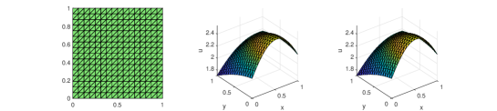
Fig. 1: The nodal values of exact and numerical solutions for the model problem

The test script can be easily used to compute $\mathbb{P}_{i}$-Lagrange element for $i=1,2,3$ (see Line 18 in the test script). The nodal values for the model problem are displayed in Fig. 1. The rates of convergence are shown in Fig. 2, from which we observe the optimal convergence for all cases.

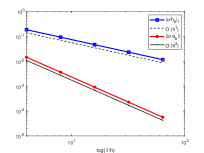
(a) $i=1$

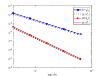
(b) $i=2$

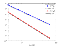
(c) $i=3$

Fig. 2: Convergence rates for the model problem.

We also print the errors on the Matlab command window, with the results for $\mathbb{P}_{3}$ element given below:

        Table: Error
            #Dof        h         ||u-u_h||      |u-u_h|_1
            ____    _________    ___________    ___________

              32    2.500e-01    2.53816e-05    5.28954e-04
             128    1.250e-01    1.53744e-06    6.50683e-05
             512    6.250e-02    9.46298e-08    8.07922e-06
            2048    3.125e-02    5.87001e-09    1.00695e-06
            8192    1.562e-02    3.65444e-10    1.25698e-07

We next consider the example with a circular domain or an L-shaped domain. Such a domain can be generated by using the pdetool as

⬇

1%% Generate an intitial mesh

2g = 'circleg'; %'lshapeg';

3[p,e,t] = initmesh(g,'hmax',0.5);

4node = p'; elem = t(1:3,:)';

5bdStr = 'x>0'; % string for Neumann

The results are given in Fig. 3

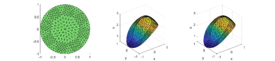
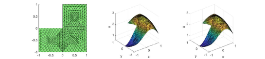
Fig. 3: The nodal values of exact and numerical solutions on circular domain or L-shaped region.

3.2 Linear elasticity problems

The linear elasticity problem is

$$\begin{cases}-{\rm div}\bm{\sigma}=\bm{f}\quad&\text{in}~{}~{}~{}\Omega,\\ \bm{u}={\bm{0}}\quad&\text{on}~{}~{}~{}\Gamma_{0},\\ \bm{\sigma n}=\bm{g}\quad&\text{on}~{}~{}~{}\Gamma_{1},\end{cases}$$ (3.1)

where $\bm{n}=(n_{1},n_{2})^{T}$ denotes the outer unit vector normal to $\partial\Omega$. The constitutive relation for linear elasticity is

$$\bm{\sigma}(\bm{u})=2\mu\bm{\varepsilon}(\bm{u})+\lambda({\rm div}\bm{u})\bm{I},$$

where $\bm{\sigma}=(\sigma_{ij})$ and $\bm{\varepsilon}=(\varepsilon_{ij})$ are the second order stress and strain tensors, respectively, satisfying $\varepsilon_{ij}=\frac{1}{2}(\partial_{i}u_{j}+\partial_{j}u_{i})$, $\lambda$ and $\mu$ are the Lamé constants, $\bm{I}$ is the identity matrix, and ${\rm div}\bm{u}=\partial_{1}u_{1}+\partial_{2}u_{2}$.

3.2.1 The programming in scalar form

The vector problem can be solved in block form by using assem2d.m as scalar cases. The equilibrium equation in (3.1) can also be written in the form

$$-\mu\Delta\bm{u}-(\lambda+\mu){\text{grad}}({\rm div}\bm{u})=\bm{f}\quad{\text{in}}~{}~{}\Omega,$$ (3.2)

which is referred to as the displacement type in what follows. In this case, we only consider $\Gamma_{0}=\Gamma:=\partial\Omega$. The first term $\Delta\bm{u}$ can be treated as the vector case of the Poisson equation. The variational formulation is

$$\mu\int_{\Omega}\nabla\bm{u}\cdot\nabla\bm{v}{\rm d}x+(\lambda+\mu)\int_{\Omega}(\text{div}~{}\bm{u})(\text{div}~{}\bm{v}){\rm d}\sigma=\int_{\Omega}\bm{f}\cdot\bm{v}{\rm d}\sigma.$$

The first term of the bilinear form can be split into

$$\mu\int_{\Omega}\nabla u_{1}\cdot\nabla v_{1}\text{d}\sigma\quad\mbox{and}\quad\mu\int_{\Omega}\nabla u_{2}\cdot\nabla v_{2}\text{d}\sigma.$$

They generate the same matrix, denoted $A$, corresponding to the blocks $A_{11}$ and $A_{22}$, respectively. The computation reads

⬇

1% (v1.grad, u1.grad), (v2.grad, u2.grad)

2cf = 1;

3Coef = cf; Test = 'v.grad'; Trial = 'u.grad';

4A = assem2d(Th,Coef,Test,Trial,Vh,quadOrder);

The second term of the bilinear form has the following combinations:

$$\int_{\Omega}v_{1,x}u_{1,x}\text{d}x,\quad\int_{\Omega}v_{1,x}u_{2,y}\text{d}x,\quad\int_{\Omega}v_{2,y}u_{1,x}\text{d}x\quad\int_{\Omega}v_{2,y}u_{2,y}\text{d}x,$$

which correspond to $A_{11}$, $A_{12}$, $A_{21}$ and $A_{22}$, respectively, and can be computed as follows.

⬇

1% (v1.dx, u1.dx)

2cf = 1;

3Coef = cf; Test = 'v.dx'; Trial = 'u.dx';

4B1 = assem2d(Th,Coef,Test,Trial,Vh,quadOrder);

5% (v1.dx, u2.dy)

6cf = 1;

7Coef = cf; Test = 'v.dx'; Trial = 'u.dy';

8B2 = assem2d(Th,Coef,Test,Trial,Vh,quadOrder);

9% (v2.dy, u1.dx)

10cf = 1;

11Coef = cf; Test = 'v.dy'; Trial = 'u.dx';

12B3 = assem2d(Th,Coef,Test,Trial,Vh,quadOrder);

13% (v2.dy, u2.dy)

14cf = 1;

15Coef = cf; Test = 'v.dy'; Trial = 'u.dy';

16B4 = assem2d(Th,Coef,Test,Trial,Vh,quadOrder);

The block matrix is then given by

⬇

1% kk

2kk = [ mu*A+(lambda+mu)*B1, (lambda+mu)*B2;

3 (lambda+mu)*B3, mu*A+(lambda+mu)*B4 ];

4kk = sparse(kk);

The right-hand side has two components:

$$\int_{\Omega}f_{1}v_{1}\text{d}x\quad\mbox{and}\quad\int_{\Omega}f_{2}v_{2}\text{d}x.$$

The load vector is assembled in the following way:

⬇

1%% Assemble right hand side

2% F1

3trf = eye(2);

4Coef = @(pz) pde.f(pz)*trf(:, 1); Test = 'v.val'; % f = [f1, f2]

5F1 = assem2d(Th,Coef,Test,[],Vh,quadOrder);

6% F2

7trf = eye(2);

8Coef = @(pz) pde.f(pz)*trf(:, 2); Test = 'v.val';

9F2 = assem2d(Th,Coef,Test,[],Vh,quadOrder);

10% F

11ff = [F1; F2];

For the vector problem, we impose the Dirichlet boundary value conditions as follows.

⬇

1%% Apply Dirichlet boundary conditions

2g_D = pde.g_D;

3on = 1;

4g_D1 = @(p) g_D(p)*[1;0];

5g_D2 = @(p) g_D(p)*[0;1];

6gBc = {g_D1,g_D2};

7Vhvec = {Vh,Vh};

8u = apply2d(on,Th,kk,ff,Vhvec,gBc); % note Vhvec

Here, g_D1 is for $u_{1}$ and g_D2 is for $u_{2}$. Note that the finite element spaces Vhvec must be given in the same structure of gBc.

The solutions are displayed in Fig. 4.

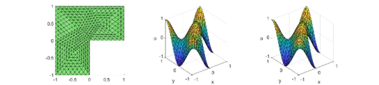
Fig. 4: The nodal values of exact and numerical solutions for the elasticity problem of displacement type.

3.2.2 The programming in vector form

The bilinear form is

$$a(\bm{v},\bm{u})=2\mu\int_{\Omega}\varepsilon_{ij}(\bm{v})\varepsilon_{ij}(\bm{u}){\rm d}\sigma+\lambda\int_{\Omega}(\partial_{i}v_{i})(\partial_{j}u_{j}){\rm d}\sigma,$$

where the summation is ommited. The computation of the first term has been given in Subsect. 2.3.2, i.e.,

⬇

1% (Eij(u):Eij(v))

2Coef = { 1, 1, 0.5 };

3Test = {'v1.dx', 'v2.dy', 'v1.dy + v2.dx'};

4Trial = {'u1.dx', 'u2.dy', 'u1.dy + u2.dx'};

5A = int2d(Th,Coef,Test,Trial,Vh,quadOrder);

6A = 2*mu*A;

The second term can be computed as

⬇

1% (div u,div v)

2Coef = 1;

3Test = 'v1.dx + v2.dy' ;

4Trial = 'u1.dx + u2.dy';

5B = int2d(Th,Coef,Test,Trial,Vh,quadOrder);

6B = lambda*B;

7% stiffness matrix

8kk = A + B;

The linear form is

$$\ell(\bm{v})=\int_{\Omega}\bm{f}\cdot\bm{v}{\rm d}\sigma+\int_{\Gamma_{1}}\bm{g}\cdot\bm{v}{\rm d}s.$$

For the first term, one has

⬇

1Coef = pde.f; Test = 'v.val';

2ff = int2d(Th,Coef,Test,[],Vh,quadOrder);

Note that we have added the implementation for $\bm{f}\cdot\bm{v}$ by just setting Test = 'v.val'. For the second term, we first determine the one-dimensional edges:

⬇

1%% Get 1D mesh for boundary integrals

2bdStr = Th.bdStr;

3if $\neg$isempty(bdStr)

4 Th.elem1d = Th.bdEdgeType{1};

5 Th.elem1dIdx = Th.bdEdgeIdxType{1};

6end

The coefficient matrix for the boundary integral can be computed using interpEdgeMat.m and the Neumann condition is then realized as

⬇

1%% Assemble Neumann boundary conditions

2if $\neg$isempty(bdStr)

3 g_N = pde.g_N; trg = eye(3);

4

5 g1 = @(p) g_N(p)*trg(:,[1,3]); Cmat1 = interpEdgeMat(g1,Th,quadOrder);

6 g2 = @(p) g_N(p)*trg(:,[3,2]); Cmat2 = interpEdgeMat(g2,Th,quadOrder);

7

8 Coef = {Cmat1, Cmat2}; Test = 'v.val';

9 ff = ff + int1d(Th,Coef,Test,[],Vh,quadOrder);

10end

Here, the data g_N is stored as $g_{N}=[\sigma_{11},\sigma_{22},\sigma_{12}]$ in the structure pde.

The Dirichlet condition can be handled as the displacement type:

⬇

1%% Apply Dirichlet boundary conditions

2on = 2 - 1*isempty(bdStr);

3g_D1 = @(pz) pde.g_D(pz)*[1;0];

4g_D2 = @(pz) pde.g_D(pz)*[0;1];

5g_D = {g_D1, g_D2};

6u = apply2d(on,Th,kk,ff,Vh,g_D);

Note that Vh is of vector form.

In the test script, we set bdStr = 'y==0 | x==1'. The errors for the $\mathbb{P}_{3}$ element are listed in Tab. 1.

Tab. 1: The $L^{2}$ and $H^{1}$ errors for the elasticity problem of tensor form ($\mathbb{P}_{3}$ element)

$\sharp{\rm Dof}$	$h$	ErrL2	ErrH1
32	2.500e-01	6.82177e-04	1.34259e-02
128	1.250e-01	3.90894e-05	1.61503e-03
512	6.250e-02	2.32444e-06	1.97527e-04
2048	3.125e-02	1.42085e-07	2.44506e-05
8192	1.562e-02	8.79363e-09	3.04301e-06

3.3 Mixed FEMs for the biharmonic equation

3.3.1 The programming in scalar form

For the mixed finite element methods, we first consider the biharmonic equation with Dirichlet boundary conditions:

$$\begin{cases}\Delta^{2}u=f\quad&{\text{in}}~{}~{}\Omega\subset\mathbb{R}^{2},\\ u=\partial_{n}u=0\quad&\text{on}~{}~{}\partial\Omega.\end{cases}$$

By introducing a new variable $w=-\Delta u$, the above problem can be written in a mixed form as

$$\begin{cases}-\Delta u=w,\\ -\Delta w=f,\\ u=\partial_{n}u=0\quad\text{on}~{}~{}\partial\Omega.\end{cases}$$

The associated variational problem is: Find $(w,u)\in H^{1}(\Omega)\times{H_{0}^{1}}(\Omega)=:V\times U$ such that

$$\begin{cases}\displaystyle\int_{\Omega}\nabla u\cdot\nabla\phi{\rm d}\sigma=\int_{\Omega}w\phi{\rm d}\sigma,\quad&\phi\in H^{1}(\Omega),\\[5.69054pt] \displaystyle\int_{\Omega}\nabla w\cdot\nabla\psi{\rm d}\sigma=\int_{\Omega}f\psi{\rm d}\sigma,\quad&\psi\in H_{0}^{1}(\Omega).\end{cases}$$ (3.3)

Let

$$a(w,\phi)=-\int_{\Omega}w\phi{\rm d}\sigma\quad\mbox{and}\quad b(\phi,u)=\int_{\Omega}\nabla\phi\cdot\nabla u{\rm d}\sigma.$$

One has

$$\begin{cases}a(w,\phi)+b(\phi,u)=0,\quad&\phi\in H^{1}(\Omega)=V,\\ b(w,\psi)=(f,\psi),\quad&\psi\in H_{0}^{1}(\Omega)=U,\end{cases}$$

where $a(\cdot,\cdot):V\times V\to\mathbb{R}$ and $b(\cdot,\cdot):V\times U\to\mathbb{R}$.

The functions $u$ and $w$ will be approximated by $\mathbb{P}_{1}$-Lagrange elements. Let $N$ be the vector of global basis functions. One easily gets

$$\begin{cases}\bm{\phi}^{T}A\bm{w}+\bm{\phi}^{T}B\bm{u}=0,\\ \bm{\psi}^{T}B^{T}\bm{w}=\bm{\psi}^{T}\bm{f},\end{cases}$$

where

$$A=-\int_{\Omega}N^{T}N{\rm d}\sigma,\qquad B=\int_{\Omega}\nabla N^{T}\cdot\nabla N{\rm d}\sigma,\qquad\bm{f}=\int_{\Omega}N^{T}f{\rm d}\sigma.$$

The system can be written in block matrix form as

$$\begin{bmatrix}A&B\\ B^{T}&O\end{bmatrix}\begin{bmatrix}\bm{w}\\ \bm{u}\end{bmatrix}=\begin{bmatrix}\bm{0}\\ \bm{f}\end{bmatrix}.$$

Remark 3.1.

If $\partial_{n}u$ does not vanish on $\partial\Omega$, then the mixed variational formulation is

$$\begin{cases}\displaystyle a(w,\phi)+b(\phi,u)=\int_{\partial\Omega}\partial_{n}u\phi{\rm d}s,\quad\phi\in V,\\ b(w,\psi)=(f,\psi),\quad\psi\in U.\end{cases}$$

Here, $\partial_{n}u$ corresponds to the Neumann boundary data for $u$ in the first equation.

In block form, the stiffness matrix can be computed as follows.

⬇

1%% Assemble stiffness matrix

2% matrix A

3Coef = 1; Test = 'v.val'; Trial = 'u.val';

4A = -assem2d(Th,Coef,Test,Trial,'P1',quadOrder);

5% matrix B

6Coef = 1; Test = 'v.grad'; Trial = 'u.grad';

7B = assem2d(Th,Coef,Test,Trial,'P1',quadOrder);

8% kk

9O = zeros(size(B));

10kk = [A, B; B', O];

11kk = sparse(kk);

The right-hand side is given by

⬇

1%% Assemble right-hand side

2Coef = pde.f; Test = 'v.val';

3ff = assem2d(Th,Coef,Test,[],'P1',quadOrder);

4O = zeros(size(ff));

5ff = [O; ff];

The computation of the Neumann boundary condition reads

⬇

1%% Assemble Neumann boundary condition

2Th.elem1d = Th.bdEdge; % all boundary edges

3%Th.bdEdgeIdx1 = Th.bdEdgeIdx;

4%Coef = @(p) pde.Du(p)*n;

5Coef = interpEdgeMat(pde.Du,Th,quadOrder);

6Test = 'v.val';

7ff(1:N) = ff(1:N) + assem1d(Th,Coef,Test,[],'P1',quadOrder);

We finally impose the Dirichlet boundary conation as

⬇

1%% Apply Dirichlet boundary conditions

2on = 1;

3g_D = pde.g_D;

4gBc = {[],g_D};

5Vhvec = {'P1','P1'};

6U = apply2d(on,Th,kk,ff,Vhvec,gBc); % note Vhvec

7w = U(1:N); u = U(N+1:end);

Note that the Dirichlet data is only for $u$, so we set gBc{1} = [] in Line 4.

The convergence rates for $u$ and $w$ are shown in Fig. 5, from which we clearly observe the first-order and the second-order convergence in the $H^{1}$ norm and $L^{2}$ norm for both variables.

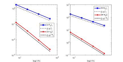
Fig. 5: The convergence rates of the mixed FEM for the biharmonic equation ($\mathbb{P}_{1}$ element)

3.3.2 The programming in vector form

Let $u_{1}=w$, $u_{2}=u$, $v_{1}=\phi$ and $v_{2}=\psi$. Then the problem (3.3) can be regarded as a variational problem of vector form, with $\bm{u}=(u_{1},u_{2})^{T}$ being the trial function and $\bm{v}=(v_{1},v_{2})^{T}$ being the test function. One easily finds that the mixed form (3.3) is equivalent to the following vector form

$$\int_{\Omega}(-v_{1}u_{1}+\nabla v_{1}\cdot\nabla u_{2}+\nabla v_{2}\cdot\nabla u_{1})\text{d}\sigma=\int_{\Omega}fv_{2}\text{d}x+\int_{\partial\Omega}g_{2}v_{1}\text{d}s,$$

which is obtained by adding the two equations.

Using int2d.m and int1d.m, we can compute the vector $\bm{u}$ as follows.

⬇

1%% Assemble stiffness matrix

2Coef = { -1, 1, 1 };

3Test = {'v1.val', 'v1.grad', 'v2.grad'};

4Trial = {'u1.val', 'u2.grad', 'u1.grad'};

5kk = int2d(Th,Coef,Test,Trial,Vh,quadOrder);

6

7%% Assemble right hand side

8Coef = pde.f; Test = 'v2.val';

9ff = int2d(Th,Coef,Test,[],Vh,quadOrder);

10

11%% Assemble Neumann boundary conditions

12% Get 1D mesh for boundary integrals

13Th.elem1d = Th.bdEdgeType{1};

14Th.elem1dIdx = Th.bdEdgeIdxType{1};

15

16% Coef = @(p) pde.Du(p)*n;

17Coef = interpEdgeMat(pde.Du,Th,quadOrder);

18Test = 'v1.val';

19ff = ff + int1d(Th,Coef,Test,[],Vh,quadOrder);

20

21%% Apply Dirichlet boundary conditions

22g_D = { [], pde.g_D };

23on = 1;

24U = apply2d(on,Th,kk,ff,Vh,g_D);

25U = reshape(U,[],2);

26w = U(:,1); u = U(:,2);

In the above code, Vh can be chosen as {'P1', 'P1' }, {'P2', 'P2' } and {'P3', 'P3' }. The results are displayed in Fig. 6. We can find that the rate of convergence for $u$ is optimal but for $w$ is sub-optimal:

• For linear element, optimal order for $w$ is also observed.

• For $\mathbb{P}_{2}$ element, the order for $L^{2}$ is 1.5 and for $H^{1}$ is 0.5.

• For $\mathbb{P}_{3}$ element, the order for $L^{2}$ is 2.5 and for $H^{1}$ is 1.5.

Note that our results are consistent with that given in $i$FEM. Obviously, for $\mathbb{P}_{2}$ and $\mathbb{P}_{3}$ elements, the rate of $w$ has the behaviour of $\Delta u$, which is reasonable since $w=-\Delta u$.

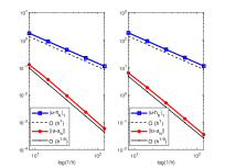
(a) P1

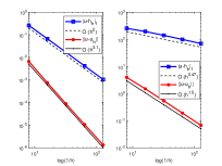
(b) P2

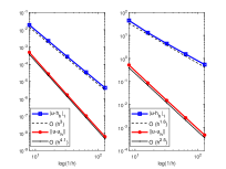
(c) P3

Fig. 6: The convergence rates for the biharmonic equation.

3.4 Mixed FEMs for the Stokes problem

The Stokes problem with homogeneous Dirichlet boundary conditions is to find $(\bm{u},p)$ such that

$$\begin{cases}-\nu\Delta\bm{u}-\nabla p=\bm{f}\quad&\mbox{in}~{}~{}\Omega,\\ {\rm div}\bm{u}=0\quad&\mbox{in}~{}~{}\Omega,\\ \bm{u}=\bm{0}\quad&\mbox{on}~{}~{}\partial\Omega.\end{cases}$$

Define $\bm{V}=\bm{H}_{0}^{1}(\Omega)$ and $P=L_{0}^{2}(\Omega)$. The mixed variational problem is: Find $(\bm{u},p)\in\bm{V}\times Q$ such that

$$\begin{cases}a(\bm{u},\bm{v})+b(\bm{v},p)&=(\bm{f},\bm{v}),\quad\bm{v}\in\bm{V},\\ b(\bm{u},q)&=0,\quad q\in P,\end{cases}$$

where

$$a(\bm{u},\bm{v})=(\nu\nabla\bm{u},\nabla\bm{v}),\qquad b(\bm{v},q)=({\rm div}\bm{v},q).$$

Let $\mathcal{T}_{h}$ be a shape regular triangulation of $\Omega$. We consider the conforming finite element discretizations: $\bm{V}_{h}\subset\bm{V}$ and $P_{h}\subset P$. Typical pairs $(\bm{V}_{h},P_{h})$ of stable finite element spaces include: MINI element, Girault-Raviart element and $\mathbb{P}_{k}-\mathbb{P}_{k-1}$ elements. For the last one, a special example is the $\mathbb{P}_{2}-\mathbb{P}_{1}$ element, also known as the Taylor-Hood element, which is the one under consideration.

The FEM is to find $(\bm{u}_{h},p_{h})\in\bm{V}_{h}\times P_{h}$ such that

$$\begin{cases}a(\bm{u}_{h},\bm{v})+b(\bm{v},p_{h})=F(\bm{v}),\quad&\bm{v}\in\bm{V}_{h},\\ b(\bm{u}_{h},q)=0,\quad&q\in P_{h}.\end{cases}$$ (3.4)

The problem (3.4) can be solved either by discretizing it directly into a system of equations (a saddle point problem), or by adding the two equations, as done for the biharmonic equation. We consider the latter one: Find $(\bm{u}_{h},p_{h})\in\bm{V}_{h}\times L^{2}(\Omega)$ such that

$$a(\bm{u}_{h},\bm{v})+b(\bm{v},p_{h})+b(\bm{u}_{h},q)-\varepsilon(p_{h},q)=F(\bm{v}),\bm{v}\in\bm{V}_{h},\quad\in L^{2}(\Omega),$$ (3.5)

where $\varepsilon$ is a small parameter to ensure stability.

The bilinear form can be assembled as follows.

⬇

1Vh = {'P2','P2','P1'}; quadOrder = 5;

2

3%% Assemble stiffness matrix

4vstr = {'v1','v2','q'}; ustr = {'u1','u2','p'};

5% [v1,v2,q] = [v1,v2,v3], [u1,u2,p] = [u1,u2,u3]

6% a1(v1,u1) + a2(v2,u2)

7% + b1(v1,p) + b2(v2,p)

8% + b1(q,u1) + b2(q,u2) - eps*(q,p)

9eps = 1e-10;

10Coef = { 1, 1, -1,-1, -1,-1, -eps};

11Test = {'v1.grad', 'v2.grad', 'v1.dx', 'v2.dy', 'q.val', 'q.val', 'q.val'};

12Trial = {'u1.grad', 'u2.grad', 'p.val', 'p.val', 'u1.dx', 'u2.dy', 'p.val'};

13[Test,Trial] = getStdvarForm(vstr, Test, ustr, Trial); % [u1,u2,p] --> [u1,u2,u3]

14[kk,info] = int2d(Th,Coef,Test,Trial,Vh,quadOrder);

Note that the symbols p and q correspond to u3 and v3, which is realized by using the subroutine getStdvarForm.m.

The computation of the right-hand side reads

⬇

1%% Assemble right hand side

2trf = eye(2);

3Coef1 = @(pz) pde.f(pz)*trf(:, 1); Coef2 = @(pz) pde.f(pz)*trf(:, 2);

4Coef = {Coef1, Coef2};

5Test = {'v1.val', 'v2.val'};

6ff = int2d(Th,Coef,Test,[],Vh,quadOrder);

In this case, one can not use Coef = pde.f and Test = 'v.val' instead since $\bm{v}=[v_{1},v_{2},v_{3}]^{T}$ has three components.

We impose the Dirichlet boundary conditions as follows.

⬇

1%% Apply Dirichlet boundary conditions

2tru = eye(2);

3g_D1 = @(pz) pde.g_D(pz)*tru(:, 1);

4g_D2 = @(pz) pde.g_D(pz)*tru(:, 2);

5g_D = {g_D1, g_D2, []};

6on = 1;

7U = apply2d(on,Th,kk,ff,Vh,g_D);

8NNdofu = info.NNdofu;

9id1 = NNdofu(1); id2 = NNdofu(1)+ NNdofu(2);

10uh = [ U(1:id1), U(id1+1:id2) ]; % uh = [u1h, u2h]

11ph = U(id2+1:end);

Note that g_D{3} = [] since no constraints are imposed on $p$.

Example 3.1.

Let $\Omega=(0,1)^{2}$. We choose the load term $\bm{f}$ in such a way that the analytical solution is

$$\bm{u}(x,y)=\begin{bmatrix}-2^{8}(x^{2}-2x^{3}+x^{4})(2y-6y^{2}+4y^{3})\\ 2^{8}(2x-6x^{2}+4x^{3})(y^{2}-2y^{3}+y^{4})\end{bmatrix}$$

and $p(x,y)=-2^{8}(2-12x+12x^{2})(y^{2}-2y^{3}+y^{4})$.

The results are displayed in Fig. 7 and Tab. 2, from which we observe the optimal rates of convergence both for $u$ and $p$.

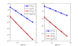
Fig. 7: Convergence rates of the Taylor-Hood element for the Stokes problem

Tab. 2: The discrete errors for the Stokes problem

$\sharp$Dof	$h$	$\|u-u_{h}\|$	$|u-u_{h}|_{1}$	$\|p-p_{h}\|$
32	2.500e-01	8.88464e-02	2.52940e+00	1.59802e+00
128	1.250e-01	1.01868e-02	6.62003e-01	3.36224e-01
512	6.250e-02	1.21537e-03	1.67792e-01	7.88512e-02
2048	3.125e-02	1.50235e-04	4.21077e-02	1.94079e-02
8192	1.562e-02	1.87368e-05	1.05374e-02	4.83415e-03

3.5 Time-dependent problems

As an example, we consider the heat equation:

$$\begin{cases}u_{t}-\Delta u=f&\mbox{in}~{}~{}\Omega,\\ u(x,y,0)=u_{0}(x,y)&\mbox{in}~{}~{}\Omega,\\ u=g_{D}&\mbox{on}~{}~{}\Gamma_{D},\\ \partial_{n}u=g_{N}&\mbox{on}~{}~{}\Gamma_{N}.\end{cases}$$

After applying the backward Euler discretization in time, we shall seek $u^{n}(x,y)$ satisfying for all $v\in H_{0}^{1}(\Omega)$:

$$\int_{\Omega}\Big{(}\frac{u^{n}-u^{n-1}}{\Delta t}v+\nabla u^{n}\cdot\nabla v\Big{)}{\rm d}\sigma=\int_{\Omega}f^{n}v{\rm d}\sigma+\int_{\Gamma_{N}}g_{N}^{n}v{\rm d}s.$$

We fist generate a mesh and compute the mesh information.

⬇

1%% Mesh

2% generate mesh

3Nx = 10;

4[node,elem] = squaremesh([0 1 0 1],1/Nx);

5% mesh info

6bdStr = 'x==0'; % Neumann

7Th = FeMesh2d(node,elem,bdStr);

8% time

9Nt = Nx^2;

10t = linspace(0,1,Nt+1)'; dt = t(2)-t(1);

The PDE data is given by

⬇

1%% PDE data

2pde = heatData();

The exact solution is chosen as $u=\sin(\pi x)\sin(y)\mathrm{e}^{-t}$.

For fixed $\Delta t$, the bilinear form gives the same stiffness matrix in each iteration.

⬇

1%% Backward Euler

2u0 = @(p) pde.uexact(p,t(1));

3uh0 = interp2d(u0,Th,Vh); % dof vector

4uf = zeros(Nt+1,2); % record solutions at p-th point

5p = 2*Nx;

6uf(1,:) = [uh0(p),uh0(p)];

7for n = 1:Nt

8 % Linear form

9 fun = @(p) pde.f(p, t(n+1));

10 Coef = fun; Test = 'v.val';

11 ff = assem2d(Th,Coef,Test,[],Vh,quadOrder);

12 Coef = uh0/dt;

13 ff = ff + assem2d(Th,Coef,Test,[],Vh,quadOrder);

14

15 % Neumann boundary condition

16 if $\neg$isempty(bdStr)

17 Th.elem1d = Th.bdEdgeType{1};

18 Th.elem1dIdx = Th.bdEdgeIdxType{1};

19 fun = @(p) pde.Du(p,t(n+1));

20 Coef = interpEdgeMat(fun,Th,quadOrder);

21 ff = ff + assem1d(Th,Coef,Test,[],Vh,quadOrder);

22 end

23

24 % Dirichlet boundary condition

25 ue = @(p) pde.uexact(p,t(n+1));

26 on = 2 - 1*isempty(bdStr); % on = 1 for the whole boundary if bdStr = []

27 uh = apply2d(on,Th,kk,ff,Vh,ue);

28

29 % Record

30 uhe = interp2d(ue,Th,Vh);

31 uf(n+1,:) = [uhe(p), uh(p)];

32

33 % Update

34 uh0 = uh;

35end

In the above code, we record solutions at $p$-th point, where $p=2N_{x}$. The results are shown in Fig. 8 and Fig. 9.

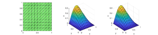
Fig. 8: Exact and numerical solutions for the heat equation

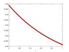
Fig. 9: Exact and numerical solutions at a fixed point for the heat equation

It is well-known that the error behaves as $\mathcal{O}(\Delta t+h^{k+1})$ for the $\mathbb{P}_{k}$-Lagrange element. To test the convergence order w.r.t $h$, one can set $\Delta t=\mathcal{O}(h^{k+1})$. The numerical results are consistent with the theoretical prediction as shown in Fig. 10.

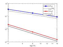
(a) P1

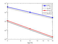
(b) P2

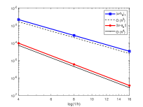
(c) P3

Fig. 10: Convergence rates for the heat equation.

4 Examples in FreeFEM Documentation

We in this section present five examples given in FreeFEM. Many more examples can be found or will be added in the example folder in varFEM.

4.1 Membrane

This is an exmple given in FreeFEM Documentation: Release 4.6 (see Subsection 2.3 - Membrane).

The equation is simply the Laplace equation, where the region is an ellipse with the length of the semimajor axis $a=2$, and unitary the semiminor axis. The mesh on such a domain can be generated by using the pdetool:

⬇

1%% Mesh

2% ellipse with a = 2, b = 1

3a = 2; b = 1;

4g = ellipseg(a,b);

5[p,e,t] = initmesh(g,'hmax',0.2);

6[p,e,t] = refinemesh(g,p,e,t);

7node = p'; elem = t(1:3,:)';

8figure,

9subplot(1,2,1),

10showmesh(node,elem);

11% bdStr

12bdNeumann = 'y<0 & x>-sin(pi/3)'; % string for Neumann

13% mesh info

14Th = FeMesh2d(node,elem,bdNeumann);

The Neumann boundary condition is imposed on

$$\Gamma_{2}=\{(x,y):x=a\cos t,~{}~{}y=b\sin t,\quad t\in(\theta,2\pi)\},\qquad\theta=4\pi/3,$$

which can be identified by setting bdStr = 'y<0 & x>-sin(pi/3)' as done in the code.

The remaining implementation is very simple, so we omit the details. The nodal values are shown in Fig. 11a.

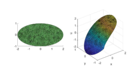
(a) Nodal values

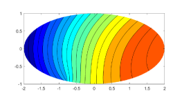
(b) Level lines

Fig. 11: Membrane deformation

We can also plot the level lines of the membrane deformation, as given in Fig. 11b. Note that the contour figure is obtained by interpolating the finite element function to a two-dimensional cartesian grid (within the mesh). The interpolated values can be created by using the Matlab build-in function pdeInterpolant.m in the pdetool. However, the build-in function seems not efficient. For this reason, we provide a new realization of the interpolant, named varInterpolant2d.m. With this function, we give a subroutine varcontourf.m to draw a contour plot.

4.2 Heat exchanger

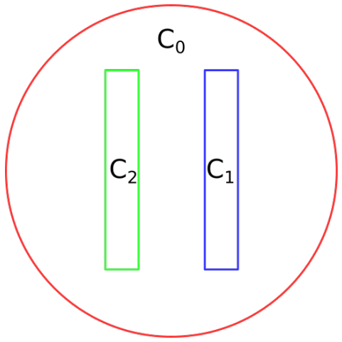
Fig. 12: Heat exchanger geometry (see [2])

The geometry is shown in Fig. 12, where $C_{1}$ and $C_{2}$ are two thermal conductors within an enclosure $C_{0}$. The temperature $u$ satisfies

$$\nabla\cdot(\kappa\nabla u)=0\quad\mbox{in}~{}~{}\Omega.$$

• The first conductor is held at a constant temperature $u_{1}=100^{\circ}{\rm C}$, and the border of enclosure $C_{0}$ is held at temperature $20^{\circ}{\rm C}$. This means the domain is $\Omega=C_{0}\backslash C_{1}$, and the boundaries consist of $\partial C_{0}$ and $\partial C_{1}$.

• The conductor $C_{2}$ has a different thermal conductivity than the enclosure $C_{0}$: $\kappa_{0}=1$ and $k_{2}=3$.

We use the mesh generated by FreeFEM, which is saved in a .msh file named meshdata_heatex.msh. The command in FreeFEM can be written as

⬇

1savemesh(Th, "meshdata_heatex.msh");

We read the basic data structures node and elem via a self-written function:

⬇

1[node,elem] = getMeshFreeFEM('meshdata_heatex.msh');

Then the mesh data can be computed as

⬇

1% bdStr

2C0 = 'x.^2 + y.^2 > 3.8^2'; % 1

3bdStr = C0;

4% mesh info

5Th = FeMesh2d(node,elem,bdStr);

Note that the remaining boundary is $\partial C_{1}$, hence the boundaries of $C_{0}$ and the first conductor are labelled as 1 and 2, respectively.

The coefficient $\kappa$ can be written as

⬇

1%% PDE data

2kappa = @(p) 1 + 2*(p(:,1)<-1).*(p(:,1)>-2).*(p(:,2)<3).*(p(:,2)>-3); % p = [x,y]

And the bilinear form and the linear form are assembled as follows.

⬇

1%% Bilinear form

2Vh = 'P1'; quadOrder = 5;

3Coef = kappa;

4Test = {'v.grad'}; Trial = {'u.grad'};

5kk = assem2d(Th,Coef,Test,Trial,Vh,quadOrder);

6

7%% Linear form

8ff = zeros(size(kk,1),1);

The Dirichlet boundary conditions are imposed in the following way:

⬇

1%% Dirichlet boundary conditions

2on = [1,2];

3gBc1 = @(p) 20+0*p(:,1);

4gBc2 = @(p) 100+0*p(:,1);

5uh = apply2d(on,Th,kk,ff,Vh,gBc1,gBc2);

Here, gBc1 is for $\partial C_{0}$ or on(1), and gBc2 is for $\partial C_{1}$ or on(2).

In FreeFEM, the numerical solution can be outputted using the command ofstream:

⬇

1ofstream file("sol_heatex.txt");

2file<<u[]<<endl;

The saved information is then loaded by

⬇

1uff = solFreeFEM('sol_heatex.txt');

The results are shown in Fig. 13, from which we observe that the varFEM solution is well matched with the one given by FreeFEM.

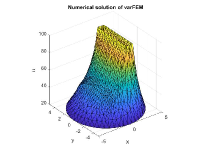
(a) varFEM

(b) FreeFEM

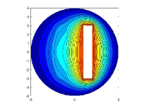
(c) Level lines

Fig. 13: Numerical solutions given by varFEM and FreeFEM

4.3 Airfoil

This is an exmple given in FreeFem Documentation: Release 4.6 (Subsection 2.7 - Irrotational Fan Blade Flow and Thermal effects).

Consider a wing profile $S$ (the NACA0012 Airfoil) in a uniform flow. Infinity will be represented by a large circle $C$ where the flow is assumed to be of uniform velocity. The domain is outside $S$, with the mesh shown in Fig. 14. The NACA0012 airfoil is a classical wing profile in aerodynamics, whose equation for the upper surface is

$$y=0.17735\sqrt{x}-0.075597x-0.212836x^{2}+0.17363x^{3}-0.06254x^{4}.$$

With this equation, we can generate a mesh using the Matlab pdetool, as included in varFEM. The function is mesh_naca0012.m. For comparison, we use the mesh generated by FreeFEM.

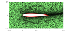
Fig. 14: Mesh zoomed around the NACA0012 airfoil

The programming is very simple, given by

⬇

1%% Parameters

2theta = 8*pi/180;

3lift = theta*0.151952/0.0872665; % lift approximation formula

4uinfty1 = cos(theta); uinfty2 = sin(theta);

5

6%% Mesh

7[node,elem] = getMeshFreeFEM('meshdata_airfoil.msh');

8% mesh info

9bdStr = 'x.^2 + y.^2 > 4.5^2'; % 1-C

10Th = FeMesh2d(node,elem,bdStr);

11

12%% Bilinear form

13Vh = 'P2'; quadOrder = 7;

14Coef = 1;

15Test = 'v.grad';

16Trial = 'u.grad';

17kk = assem2d(Th,Coef,Test,Trial,Vh,quadOrder);

18

19%% Linear form

20ff = zeros(size(kk,1),1);

21

22%% Dirichlet boundary conditions

23on = [1,2];

24gBc1 = @(p) uinfty1*p(:,2) - uinfty2*p(:,1); % on 1-C

25gBc2 = @(p) -lift + 0*p(:,1); % on 2-S

26uh = apply2d(on,Th,kk,ff,Vh,gBc1,gBc2);

We refer the reader to the FreeFEM Documentation for more details (The code is potential.edp in the software). The zoomed solutions of the streamlines are shown in Fig. 15, where the varFEM solution is well matched with the one given by FreeFEM.

(a) varFEM solution

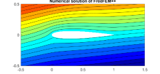
(b) FreeFEM solution

Fig. 15: Zoom around the NACA0012 airfoil showing the streamlines

4.4 Newton method for the steady Navier-Stokes equations

For the introduction of the problem, please refer to FreeFEM Documentation (Subsect. 2.12 - Newton Method for the Steady Navier-Stokes equations).

In each iteration, one needs to solve the following variational problem: Find $(\delta\bm{u},\delta p)$ such that

$$DF(\delta\bm{u},\delta p;\bm{u},p)=F(\bm{u},p),$$

where $\bm{u}$ and $p$ are the solutions given in the last step, and

$$DF(\delta\bm{u},\delta p;\bm{u},p)=\int_{\Omega}((\delta\bm{u}\cdot\nabla)\bm{u})\cdot\bm{v}+((\bm{u}\cdot\nabla)\delta\bm{u})\cdot\bm{v}+\nu\nabla\delta\bm{u}:\nabla v-q\nabla\cdot\delta\bm{u},$$

$$F(\bm{u},p)=\int_{\Omega}((\bm{u}\cdot\nabla)\bm{u})\cdot\bm{v}+\nu\nabla\bm{u}:\nabla v-p\nabla\bm{u}:\nabla\bm{v}-q\cdot\bm{u},$$

where $(\bm{v},q)$ are the test functions.

The finite element spaces and the quadrature rule are

⬇

1Vh = {'P2','P2','P1'}; % v = [v1,v2,q] --> [v1,v2,v3]

2quadOrder = 7;

3vstr = {'v1','v2','q'}; ustr = {'du1','du2','dp'};

Here vstr and ustr are for the test and trial functions, respectively.

In the following, we only provide the detail for the assembly of the first term of $DF$, i.e.,

$$\int_{\Omega}((\delta\bm{u}\cdot\nabla)\bm{u})\cdot\bm{v}=\int_{\Omega}u_{1,x}\cdot v_{1}\delta u_{1}+u_{1,y}\cdot v_{1}\delta u_{2}+u_{2,x}\cdot v_{2}\delta u_{1}+u_{2,y}\cdot v_{2}\delta u_{2}.$$ (4.1)

In the iteration, $u_{1,x}$, $u_{1,y}$, $u_{2,x}$ and $u_{2,y}$ are the known coefficients, which can be obtained from the finite element function $\bm{u}$ in the last step. Let us discuss the implementation of varFEM:

• The initial data are

  ⬇

  1% initial data

  2u1 = @(p) double( (p(:,1).^2 + p(:,2).^2 > 2) );

  3u2 = @(p) 0*p(:,1);

  4p = @(p) 0*p(:,1);

  We must convert them into the dof vectors in view of the iteration.

  ⬇

  1uh1 = interp2d(u1,Th,Vh{1});

  2uh2 = interp2d(u2,Th,Vh{2});

  3ph = interp2d(p,Th,Vh{3});

• For numerical integration, it is preferable to provide the coefficient matrices for these coefficient functions.

  ⬇

  1u1c = interp2dMat(uh1,'u1.val',Th,Vh{1},quadOrder);

  2u2c = interp2dMat(uh2,'u2.val',Th,Vh{2},quadOrder);

  3pc = interp2dMat(ph,'p.val',Th,Vh{3},quadOrder);

  4

  5u1xc = interp2dMat(uh1,'u1.dx',Th,Vh{1},quadOrder);

  6u1yc = interp2dMat(uh1,'u1.dy',Th,Vh{1},quadOrder);

  7u2xc = interp2dMat(uh2,'u2.dx',Th,Vh{2},quadOrder);

  8u2yc = interp2dMat(uh2,'u2.dy',Th,Vh{2},quadOrder);

  Here, interp2dMat.m provides a way to get the coefficient matrices only from the dof vectors.

• The triple (Coef,Test,Trial) for (4.1) is then given by

  ⬇

  1Coef = { u1xc, u1yc, u2xc, u2yc};

  2Test = { 'v1.val', 'v1.val', 'v2.val', 'v2.val'};

  3Trial = { 'du1.val', 'du2.val', 'du1.val', 'du2.val'};

  A complete correspondence of $DF(\delta\bm{u},\delta p;\bm{u},p)$ can be listed in the following:

  ⬇

  1Coef = { u1xc, u1yc, u2xc, u2yc, ... % term 1

  2 u1c, u2c, u1c, u2c, ... % term 2

  3 nu, nu, nu, nu, ... % term 3

  4 -1, -1, ... % term 4

  5 -1, -1, ... % term 5

  6 -eps ... % stablization term

  7 };

  8Test = { 'v1.val', 'v1.val', 'v2.val', 'v2.val', ... % term 1

  9 'v1.val', 'v1.val', 'v2.val', 'v2.val', ... % term 2

  10 'v1.dx', 'v1.dy', 'v2.dx', 'v2.dy', ... % term 3

  11 'v1.dx', 'v2.dy', ... % term 4

  12 'q.val', 'q.val', ... % term 5

  13 'q.val' ... % stablization term

  14 };

  15Trial = { 'du1.val', 'du2.val', 'du1.val', 'du2.val',... % term 1

  16 'du1.dx', 'du1.dy', 'du2.dx', 'du2.dy', ... % term 2

  17 'du1.dx', 'du1.dy', 'du2.dx', 'du2.dy', ... % term 3

  18 'dp.val', 'dp.val', ... % term 4

  19 'du1.dx', 'du2.dy', ... % term 5

  20 'dp.val' ... % stablization term

  21 };

• The computation of the stiffness matrix reads

  ⬇

  1[Test,Trial] = getStdvarForm(vstr, Test, ustr, Trial);

  2[kk,info] = int2d(Th,Coef,Test,Trial,Vh,quadOrder);

  Here getStdvarForm.m transforms the user-defined notation to the standard one.

The complete test script is available in test_NSNewton.m. The varFEM solutions and the FreeFEM solutions are shown in Fig. 16.

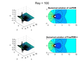
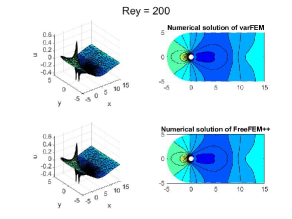
Fig. 16: The pressure $p$ of a flow

4.5 Optimal control

4.5.1 The gradient is not provided

This is an exmple given in FreeFem Documentation: Release 4.6 (Subsection 2.15 - Optimal Control).

For a given target $u_{d}$, the problem is to find $u$ such that

$$\min_{z\in\mathbb{R}^{3}}J(z)=\int_{E}(u-u_{d})^{2}=\int_{\Omega}I_{E}(u-u_{d})^{2},\quad z=(b,c,d),$$

where $E\subset\Omega$, $I_{E}$ is an indication function, and $u$ is the solution of the following PDE:

$$\begin{cases}-\nabla(\kappa(b,c,d)\cdot\nabla u)=0&\mbox{in}~{}~{}\Omega,\\ u=u_{\Gamma}&\mbox{on}~{}~{}\Gamma\subset\partial\Omega.\end{cases}$$

Let $B,C$ and $D$ be the separated subsets of $\Omega$. The coefficient $\kappa$ is defined as

$$\kappa(x)=1+bI_{B}(x)+cI_{C}(x)+dI_{D}(x),\quad x\in\Omega.$$

For fixed $z=(b,c,d)$, one can solve the PDE to obtain an approximate solution $u_{h}$ and the approximate objective function:

$$J_{h}(z,u_{h},u_{d}):=\int_{\Omega}I_{E}(u_{h}(z)-u_{d})^{2}.$$

We use the build-in function fminunc.m in Matlab to find the (local) minimizer. To this end, we first establish a function to get the PDE solution:

⬇

1%% Problem for the PDE constraint

2function uh = PDEcon(z,Th)

3

4 % Parameters

5 Vh = Th.Vh; quadOrder = Th.quadOrder;

6 Ib = @(p) (p(:,1).^2 + p(:,2).^2 < 1.0001);

7 Ic = @(p) ( (p(:,1)+3).^2 + p(:,2).^2 < 1.0001);

8 Id = @(p) (p(:,1).^2 + (p(:,2)+3).^2 < 1.0001);

9

10

11 % Bilinear form

12 Coef = @(p) 1 + z(1)*Ib(p) + z(2)*Ic(p) + z(3)*Id(p);

13 Test = 'v.grad';

14 Trial = 'u.grad';

15 kk = assem2d(Th,Coef,Test,Trial,Vh,quadOrder);

16

17 % Linear form

18 ff = zeros(size(kk,1),1);

19

20 % Dirichlet boundary condition

21 gD = @(p) p(:,1).^3 - p(:,2).^3;

22 on = 1;

23 uh = apply2d(on,Th,kk,ff,Vh,gD);

24end

The cost function is then given by

⬇

1%% Cost function

2function err = J(z,ud,Th)

3 Ie = @(p) ((p(:,1)-1).^2 + p(:,2).^2 $\leq$4);

4 uh = PDEcon(z,Th);

5

6 fh = Ie(Th.node).*(uh-ud).^2;

7 err = integral2d(Th,fh,Th.Vh,Th.quadOrder);

8end

Given a vector $z_{d}=[2,3,4]$, we can construct an “exact solution” solution $u_{d}$ by solving the PDE. The minimizer is then given by

⬇

1%% The constructed solution

2zd = [2, 3, 4];

3ud = PDEcon(zd,Th);

4

5%% Find the mimimizer

6options.LargeScale = 'off';

7options.HessUpdate = 'bfgs';

8options.Display = 'iter';

9z0 = [1,1,1];

10zmin = fminunc(@(z) J(z,ud,Th), z0, options)

In the Matlab command window, one can get the following information:

                                                             First-order
      Iteration  Func-count       f(x)        Step-size       optimality
          0           4          30.9874                          77.2
          1           8          9.87548      0.0129606           21.4
          2          12          6.27654              1           12.2
          3          16          4.76889              1            5.3
          4          20          4.47092              1           3.03
          5          24          3.46888              1           5.66
          6          28          2.13699              1           5.77
          7          32          1.06649              1           4.42
          8          36         0.542858              1           3.14
          9          40         0.295327              1           2.18
         10          44         0.179846              1            1.7
         11          48         0.114221              1           1.28
         12          52         0.063295              1          0.842
         13          56        0.0242571              1          0.366
         14          60       0.00729547              1          0.258
         15          64       0.00170544              1          0.107
         16          68      3.95891e-05              1         0.0257
         17          72      3.54227e-07              1        0.00546
         18          76      3.36066e-10              1       0.000159
         19          80      5.54979e-13              1       3.88e-06

     Local minimum found.

     Optimization completed because the size of the gradient is less than
     the value of the optimality tolerance.

     <stopping criteria details>

     zmin =

         2.0000    3.0000    4.0000

We can observe that the minimizer is found after 19 iterations, with the solutions displayed in Fig. 17.

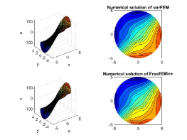
Fig. 17: Numerical solutions of the optimal control problem

4.5.2 The gradient is provided

For the example given in FreeFEM, the optimization problem is solved by the quasi-Newton BFGS method:

⬇

1BFGS(J, DJ, z, eps=1.e-6, nbiter=15, nbiterline=20);

Here, DJ is the derivatives of $J$ with respect to $b,c,d$. We also provide an implementation when the gradient is available. In this case, the cost function should be modified as

⬇

1function [err,derr] = J(z,ud,Th)

2end

Here err and derr correspond J and DJ, respectively. For the details of the implementation, please refer to the test script test_optimalControlgrad.m in varFEM. The minimizer is then captured as follows.

⬇

1%% Find the mimimizer

2options = optimoptions('fminunc','Display','iter',...

3 'SpecifyObjectiveGradient',true); % gradient is provided

4z0 = [1,1,1];

5zmin = fminunc(@(z) J(z,ud,Th), z0, options)

Note that Line 3 indicates that the gradient is provided.

The minimizer is also found, with the printed information given as

      Iteration  Func-count       f(x)        Step-size       optimality
          0           1          30.9874                          77.2
          1           2          9.87549      0.0129606           21.4
          2           3          6.27653              1           12.2
          3           4          4.76889              1            5.3
          4           5          4.47091              1           3.03
          5           6          3.46888              1           5.66
          6           7            2.137              1           5.77
          7           8          1.06648              1           4.42
          8           9         0.542849              1           3.14
          9          10         0.295333              1           2.18
         10          11         0.179846              1            1.7
         11          12         0.114223              1           1.28
         12          13        0.0632962              1          0.842
         13          14        0.0242572              1          0.366
         14          15       0.00729561              1          0.258
         15          16        0.0017055              1          0.107
         16          17      3.95888e-05              1         0.0257
         17          18      3.54191e-07              1        0.00546
         18          19      3.47621e-10              1       0.000159
         19          20      4.31601e-13              1       3.87e-06

     Local minimum found.

     Optimization completed because the size of the gradient is less than
     the value of the optimality tolerance.

     <stopping criteria details>

     zmin =

         2.0000    3.0000    4.0000

Compared with the previous implementation, one can find that the latter approach has fewer function calls (although we need to compute the gradient by solving a PDE problem).

5 Concluding remarks

In this paper, a Matlab software package for the finite element method was presented for various typical problems, which realizes the programming style in FreeFEM. The usage of the library, named varFEM, was demonstrated through several examples. Possible extensions of this library that are of interest include three-dimensional problems and other types of finite elements.

References

- [1] L. Chen. iFEM: an integrated finite element method package in MATLAB. Technical report, University of California at Irvine, 2009.
- [2] F. Hecht. New development in freefem++. J. Numer. Math., 20(3-4):251–265, 2012.