Scaling ResNets in the Large-depth Regime

Abstract

Deep ResNets are recognized for achieving state-of-the-art results in complex machine learning tasks. However, the remarkable performance of these architectures relies on a training procedure that needs to be carefully crafted to avoid vanishing or exploding gradients, particularly as the depth $L$ increases. No consensus has been reached on how to mitigate this issue, although a widely discussed strategy consists in scaling the output of each layer by a factor $\alpha_{L}$. We show in a probabilistic setting that with standard i.i.d. initializations, the only non-trivial dynamics is for $\alpha_{L}=\nicefrac{{1}}{{\sqrt{L}}}$—other choices lead either to explosion or to identity mapping. This scaling factor corresponds in the continuous-time limit to a neural stochastic differential equation, contrarily to a widespread interpretation that deep ResNets are discretizations of neural ordinary differential equations. By contrast, in the latter regime, stability is obtained with specific correlated initializations and $\alpha_{L}=\nicefrac{{1}}{{L}}$. Our analysis suggests a strong interplay between scaling and regularity of the weights as a function of the layer index. Finally, in a series of experiments, we exhibit a continuous range of regimes driven by these two parameters, which jointly impact performance before and after training.

Keywords: ResNets, deep learning theory, neural ODE, neural network initialization, continuous-time models

1 Introduction

1.1 Deep residual neural networks

Residual neural networks (ResNets), introduced by He et al. (2016a) in the field of computer vision, were the first deep neural network models successfully trained with several thousand layers. Since then, extensive empirical evidence has shown that increasing the depth leads to significant improvements in performance, while raising new challenges in terms of training (e.g., Wang et al., 2022). From a high-level perspective, the key feature of ResNets is the presence of skip connections between successive layers. In mathematical terms, this means that the $(k+1)$-th hidden state $h_{k+1}\in{\mathbb{R}}^{d}$ follows sequentially from the previous hidden state via the recurrence relation

$$h_{k+1}=h_{k}+f(h_{k},\theta_{k+1}),\quad 0\leqslant k\leqslant L-1,$$ (1)

where $f(\cdot,\theta_{k+1})$ is the layer function parameterized by $\theta_{k+1}\in{\mathbb{R}}^{p}$ and $L$ is the number of layers. The skip connection corresponds to the addition of $h_{k}$ on the right-hand side of (1), which is absent in classical feedforward networks. This refinement prevents instability issues during training when $L$ is large, provided training is performed in a careful way (He et al., 2015). The idea of adding skip connections has become common practice in the field of deep learning, and is today incorporated in many other models such as Transformers in natural language processing (Vaswani et al., 2017). For simplicity, in the rest of the paper, we continue to use the terminology ResNets to denote any architecture of the form (1), keeping in mind that this framework goes beyond the original model of He et al. (2016a).

The most common architectures have 50-150 layers, but ResNets can be trained with depths up to the order of thousand layers (He et al., 2016b). Yet, the training procedure needs to be carefully crafted to avoid vanishing or exploding gradients, particularly as the depth increases. As pointed out by, e.g., Shao et al. (2020), these instabilities are related to a shift in the magnitude of the variance of a signal as it passes through the network. In the original approach of He et al. (2016a), the issue was mitigated by adding a normalization step, called batch normalization (Ioffe and Szegedy, 2015), which rescales the output of each layer via centering and unit variance normalization. However, this normalization stage introduces practical and theoretical difficulties, among which computational overhead and strong dependence on the batch size (see Brock et al., 2021, and the references therein). A widespread alternative to stabilize training in deep models, explored for example by Yang and Schoenholz (2017), Arpit et al. (2019), Zhang et al. (2019b), and De and Smith (2020), is to incorporate a scaling factor $\alpha_{L}$ in front of the residual term in (1), yielding the model

$$h_{k+1}=h_{k}+\alpha_{L}f(h_{k},\theta_{k+1}),\quad 0\leqslant k\leqslant L-1.$$ (2)

There is strong evidence that this scaling factor $\alpha_{L}$ should depend on $L$, without however any consensus to date on the exact form of this dependence, nor on the mathematical grounding of the approach. Thus, despite progresses on the empirical side, the mathematical forces in action behind the stability of deep ResNets are still poorly understood, although they are key to unlock training at arbitrary depth.

Our goal in the present paper is to take a step forward towards a better theoretical understanding of deep ResNets by providing a thorough probabilistic analysis of the sequence $(h_{k})_{0\leqslant k\leqslant L}$ at initialization when $L$ is large, and by leveraging a continuous-time interpretation of model (2) via the so-called neural ordinary differential equation (neural ODE, Chen et al., 2018) paradigm. In a nutshell, our results highlight the intimate connection that exists at initialization between stability of the learning process, the regularity of the weights, and the scaling factor $\alpha_{L}$. We offer in particular a proper mathematical grounding on why and how to choose the parameter $\alpha_{L}$ as a function of the depth $L$ and the distribution of the weights.

1.2 Our contributions

Scaling at initialization.

The optimal parameters of ResNets are learnt by minimizing some empirical risk function via a gradient descent algorithm. As highlighted for example by Yang and Schoenholz (2017), Hanin and Rolnick (2018), and Arpit et al. (2019), a good parameter initialization of this learning phase plays a major role in the quality of the learnt model, in particular to avoid vanishing gradients and deadlock at initialization, or exploding gradients and quick divergence of the model parameters at the beginning of training. Moreover, a good initialization allows the use of larger learning rates, which have been shown to correlate with better generalization (Jastrzkebski et al., 2017). It is thus of great interest to study and understand the role played by scaling of deep ResNets at initialization. This is the context in which we place ourselves in the sequel.

At initialization stage, the weights $(\theta_{k})_{1\leqslant k\leqslant L}$ are usually chosen as (realizations of) independent and identically distributed (i.i.d.) random variables, which typically follow a uniform or Gaussian distribution on ${\mathbb{R}}^{p}$. Accordingly, the sequence $(h_{k})_{0\leqslant k\leqslant L}$ that results from the recursion (2) for a given input to the network takes the form of a sequence of random variables that are not i.i.d. but are actually a martingale. Thus, denoting informally by $\mathscr{L}$ the differentiable loss associated with the learning task (classification or regression), the distributions of $(h_{k})_{0\leqslant k\leqslant L}$ and $(\frac{\partial\mathscr{L}}{\partial h_{k}})_{0\leqslant k\leqslant L}$ as $L$ becomes large carry useful information on the stability of training. For instance, exploding gradients in the backpropagation phase of learning correspond to the fact that, with high probability, $\|\frac{\partial\mathscr{L}}{\partial h_{0}}\|\gg\|\frac{\partial\mathscr{L}}{\partial h_{L}}\|$, where $\|\cdot\|$ denotes the Euclidean norm. Our first contribution, in Section 2, is to provide thorough mathematical statements on the behavior of these distributions (both for finite and infinite $L$), depending on the value of $\alpha_{L}$. Among other results, we show that only the choice $\alpha_{L}\approx\nicefrac{{1}}{{\sqrt{L}}}$ yields a non-trivial behavior at initialization, thereby confirming empirical findings in the literature (Arpit et al., 2019; De and Smith, 2020). For $\alpha_{L}\gg\nicefrac{{1}}{{\sqrt{L}}}$, the norms explode exponentially fast with $L$, which is inappropriate for training. For $\alpha_{L}\ll\nicefrac{{1}}{{\sqrt{L}}}$, the network is almost equivalent to identity, that is, $h_{L}\approx h_{0}$. The analysis of the different cases as a function of $\alpha_{L}$ is mathematically involved and makes extensive use of concentration tools from random matrix theory.

The continuous approach.

As noticed by several authors (Chen et al., 2018; Thorpe and van Gennip, 2018; E et al., 2019), model (2) with a scaling factor $\alpha_{L}=\nicefrac{{1}}{{L}}$ (and not $\nicefrac{{1}}{{\sqrt{L}}}$) is formally similar to the discretization of a differential equation. Thus, when $L$ tends to infinity, the weights and hidden states change continuously with the layer according to the equation

$$\frac{dH_{t}}{dt}=f(H_{t},\Theta_{t}),\quad t\in[0,1].$$ (3)

Here, time $t$ is the continuous analogue of the layer index $k$, $H:[0,1]\to{\mathbb{R}}^{d}$ is a continuous-time hidden state, and $\Theta:[0,1]\to{\mathbb{R}}^{p}$ a continuous-time parameter. This important connection between ResNets and differential equations has been identified in the past years under the umbrella name of neural ODE. Since the original article of Chen et al. (2018), this point of view has led to the development of a variety of new continuous-time models, together with innovative architectures and efficient training algorithms (Chang et al., 2019; Grathwohl et al., 2019; Kidger et al., 2021). The neural ODE paradigm also enabled to leverage the rich theory of differential equations to better understand the mechanisms at work behind deep ResNets (E et al., 2019; Fermanian et al., 2021). However, there is a debated question in the neural ODE community about the choice $\alpha_{L}=\nicefrac{{1}}{{L}}$, which guarantees convergence of the discrete model (2) to its continuous-time counterpart (3). As a matter of fact, it seems that this choice is guided by more mathematical than practical considerations, and several authors have suggested that it is inconsistent with what is done in practice (Cohen et al., 2021; Bayer et al., 2022). Moreover, letting $\alpha_{L}=\nicefrac{{1}}{{L}}$ is somewhat contradictory with the results discussed above, which highlighted that the only non-trivial limit at initialization is $\alpha_{L}=\nicefrac{{1}}{{\sqrt{L}}}$. Thus, as a second contribution, we clarify the problem in Section 3 by leveraging our previous results on stability. We show that the value $\alpha_{L}=\nicefrac{{1}}{{\sqrt{L}}}$ corresponds in the continuous world to a neural stochastic differential equation (SDE) of the form (3), where now $\Theta:[0,1]\to{\mathbb{R}}^{p}$ takes the form of a continuous-time stochastic process, typically a Brownian motion. By contrast, we also prove that the neural ODE regime with $\alpha_{L}=\nicefrac{{1}}{{L}}$ corresponds to the limit of a ResNet, not with i.i.d. weights as considered before, but with more complex and correlated weight distributions. For these weight distributions, the scaling $\alpha_{L}=\nicefrac{{1}}{{L}}$ is also a critical value between explosion and identity.

Going further, our third contribution is to exhibit in Section 4 a continuous range of regimes that are controlled by the choice of $\alpha_{L}$ (beyond the cases $\nicefrac{{1}}{{\sqrt{L}}}$ and $\nicefrac{{1}}{{L}}$) and the distribution of $(\theta_{k})_{1\leqslant k\leqslant L}$ at initialization, derived from a continuous-time process $\Theta$ with a regularity different from a Brownian motion. More precisely, we show experimentally that there is a strong interplay (with the same three cases—explosion, identity mapping, non-trivial behavior) between the choice of $\alpha_{L}$ and the regularity of $(\theta_{k})_{1\leqslant k\leqslant L}$ as a function of the layer index $k$. In addition, empirical evidence suggests that this interplay impacts both the behavior and performance of the networks during training, beyond initialization.

1.3 Related work

The choice of scaling for ResNets has been discussed in many papers, without however reaching a clear consensus on the form this scaling factor should take. For instance, Hanin and Rolnick (2018) state that stability requires $\alpha_{L}\leqslant\nicefrac{{1}}{{L}}$, while Zhang et al. (2019b) show that $\alpha_{L}\leqslant\nicefrac{{1}}{{\sqrt{L}}}$ is enough to ensure stability. On the other hand, Cohen et al. (2021) claim that the scaling factor observed in practice in trained ResNets is of the form $\nicefrac{{1}}{{L^{\beta}}}$ with $\beta\approx 0.7$. Other authors have proposed more complex choices for $\alpha_{L}$ (e.g., Zhang et al., 2019a; Shao et al., 2020). Taking another point of view, De and Smith (2020) observe that batch normalization is empirically equivalent to taking a $\nicefrac{{1}}{{\sqrt{L}}}$ normalization factor. Bachlechner et al. (2021) suggest to learn a scaling parameter $\alpha_{k}$ that is allowed to vary from one layer to another, whereas, in (4), $\alpha_{L}$ is kept constant across layers. These authors observe a great acceleration for training compared to traditional ResNets with no scaling. They also suggest a similar architecture for Transformers and then notice that $\alpha_{k}\approx\nicefrac{{1}}{{L}}$ at the end of training.

Closest to our analysis at initialization are the papers of Arpit et al. (2019) and Zhang et al. (2019b). Arpit et al. (2019) develop a theoretical analysis based on mean field approximation that suggests that a scaling factor $\alpha_{L}=\nicefrac{{1}}{{\sqrt{L}}}$ prevents vanishing/exploding gradients at initialization, and provide experimental evidence that this approach is competitive with batch normalization. However, the authors do not provide rigorous mathematical statements for the three different cases $\alpha_{L}\ll\nicefrac{{1}}{{\sqrt{L}}}$, $\alpha_{L}\approx\nicefrac{{1}}{{\sqrt{L}}}$, and $\alpha_{L}\gg\nicefrac{{1}}{{\sqrt{L}}}$, nor do they highlight the connection with the continuous-time interpretation. Interestingly, the idea of exploiting the martingale structure to analyze the magnitude of the hidden states is present in Zhang et al. (2019b), who study the convergence of gradient descent for over-parameterized ResNets with different values of $\alpha_{L}$. Nevertheless, they consider a specific model with Gaussian weights, and only provide asymptotic results when both width and depth tend to infinity.

The connection between the choice of scaling and the continuous-time point of view has previously been noticed by Zhang et al. (2019c), then studied in detail by Cohen et al. (2021). The latter show that, under assumptions on the form of the weights, it is possible to derive limiting (stochastic or ordinary) differential equations for the hidden states. However, they do not discuss the transition between these two regimes, nor do they link differential equations regimes with the stability of the network.

2 Scaling at initialization

Our goal in this section is to study the effect of the scaling factor $\alpha_{L}$ on the stability of ResNets at initialization, assuming that the weights are i.i.d. random variables. We start by making more precise the model and the learning problem introduced in (1).

2.1 Model and assumptions

Model.

The data is a sample of $n$ pairs $(x_{i},y_{i})_{1\leqslant i\leqslant n}$, where $x_{i}$ is the input vector in ${\mathbb{R}}^{n_{\textnormal{in}}}$ and $y_{i}\in{\mathbb{R}}^{n_{\textnormal{out}}}$ is the output vector to be predicted. This setting includes regression and classification (after one-hot encoding of the labels). Specifying the informal recurrence (1), for any input $x\in{\mathbb{R}}^{n_{\textnormal{in}}}$, we consider the output $F_{\pi}(x)\in{\mathbb{R}}^{n_{\textnormal{out}}}$ of the ResNet model defined by

$$\begin{split}h_{0}&=Ax,\\ h_{k+1}&=h_{k}+\alpha_{L}V_{k+1}g(h_{k},\theta_{k+1}),\quad 0\leqslant k\leqslant L-1,\\ F_{\pi}(x)&=Bh_{L},\end{split}$$ (4)

where $\alpha_{L}>0$ is the scaling factor of the ResNet and $\pi=(A,B,(\theta_{k})_{1\leqslant k\leqslant L},(V_{k})_{1\leqslant k\leqslant L})$ are its parameters, with $A\in{\mathbb{R}}^{d\times n_{\textnormal{in}}}$, $B\in{\mathbb{R}}^{n_{\textnormal{out}}\times d}$, $\theta_{k}\in{\mathbb{R}}^{p}$ and $V_{k}\in{\mathbb{R}}^{d\times d}$ for $k=1,\ldots,L$. The almost-everywhere differentiable function $g:{\mathbb{R}}^{d}\times{\mathbb{R}}^{p}\to{\mathbb{R}}^{d}$ encodes the choice of architecture. We note that the model includes initial and final linear layers in order to map the input space ${\mathbb{R}}^{n_{\textnormal{in}}}$ into the space of hidden states ${\mathbb{R}}^{d}$, and symmetrically to map the last hidden state $h_{L}$ into the output space ${\mathbb{R}}^{n_{\textnormal{out}}}$. These two transformations are of little interest to us, since we mostly focus on the behavior of the sequence of hidden states $(h_{k})_{0\leqslant k\leqslant L}$. Let us finally notice that the results of this section can be adapted to hidden layers that do not have the same width, at the cost of increased technicality.

An important feature of model (4) is that the layer function takes the form of a matrix-vector multiplication, which will prove crucial to make use of concentration results on random matrices. We stress that this setting is standard in practice and that it encompasses many different types of ResNets. It includes for example simple ResNets where $g(h,\theta)=\sigma(h)$ with $\sigma$ the activation function, and the original ResNets from He et al. (2016a), which have

$$g(h,\theta)=\textnormal{ReLU}(Wh+b),$$

where the parameter is a pair $\theta=(W,b)$ with $W\in{\mathbb{R}}^{d\times d}$ a weight matrix and $b\in{\mathbb{R}}^{d}$ a bias, and ReLU: $x\mapsto\max(x,0)$ is applied element-wise. This setting also includes attention layers, where $g$ corresponds to the scaled dot-product between keys and queries, as well as convolutional layers. Although the assumptions we make later have to be slightly modified to cover this context, the rationale should extend. We leave this extension for future work.

Throughout the article, we let $\ell:{\mathbb{R}}^{n_{\textnormal{out}}}\times{\mathbb{R}}^{n_{\textnormal{out}}}\rightarrow{\mathbb{R}}_{+}$ be a loss function, differentiable w.r.t. its first parameter, for example the squared loss or the cross-entropy loss. The objective of learning is to find the optimal parameter $\pi$ that minimizes the empirical risk $\mathscr{L}(\pi)=\sum_{i=1}^{n}\ell(F_{\pi}(x_{i}),y_{i})$.

Probabilistic setting at initialization.

The minimization of the empirical risk is usually performed by stochastic gradient descent or one of its variants (Goodfellow et al., 2016, Chapter 8). The gradient descent is initialized by choosing the weights as (realizations of) i.i.d. random variables. The parameters $\theta_{1},V_{1},\dots,\theta_{L},V_{L}$ in model (4) are therefore assumed to be an i.i.d. collection of random variables, where we recall that $\theta_{k}\in{\mathbb{R}}^{p}$ and $V_{k}\in{\mathbb{R}}^{d\times d}$ parameterize the $k$-th layer of the network. In this stochastic context, the successive hidden states $h_{0},\dots,h_{L}$ given a fixed input $x$ are also random variables, but their distribution is not i.i.d.—in fact, under our assumptions, this sequence is a martingale. To avoid unnecessary technicalities, we assume that the sequence $(h_{k})_{0\leqslant k\leqslant L}$ is non-atomic. This is for example the case if the distribution of the parameters is absolutely continuous w.r.t. the Lebesgue measure. In particular, this ensures that the sequence $(h_{k})_{0\leqslant k\leqslant L}$ almost surely does not hit the non-differentiability points of $g$.

It is stressed that the distribution of the parameters are assumed to be independent of the depth, so that all the dependence on $L$ is captured in the scaling factor $\alpha_{L}$. This model enables us to consider multiple architectures at once, via the function $g$. By contrast, some authors formulate the problem of scaling as a choice of the variance at initialization (e.g., Yang and Schoenholz, 2017; Wang et al., 2022), which makes the analysis architecture-dependent. However, for a given architecture, these two approaches are essentially equivalent since $\operatorname*{Var}(\alpha_{L}V_{k})=\alpha_{L}^{2}\operatorname*{Var}(V_{k})$.

The quantity $\|h_{L}-h_{0}\|/\|h_{0}\|$ carries key information on the behavior of the network at initialization. On the one hand, if $\|h_{L}-h_{0}\|\ll\|h_{0}\|$, the network is essentially equal to the identity function. On the other hand, if $\|h_{L}-h_{0}\|\gg\|h_{0}\|$, the output of the network explodes. An intermediate situation is when $\|h_{L}-h_{0}\|\approx\|h_{0}\|$. In addition, another source of information is provided by the gradients of the hidden states with respect to the empirical risk $\mathscr{L}$. If $\|\frac{\partial\mathscr{L}}{\partial h_{0}}-\frac{\partial\mathscr{L}}{\partial h_{L}}\|\ll\|\frac{\partial\mathscr{L}}{\partial h_{L}}\|$, the gradients do not change as they flow through the network, which means that the exact same information is backpropagated throughout the network. Conversely, if $\|\frac{\partial\mathscr{L}}{\partial h_{0}}-\frac{\partial\mathscr{L}}{\partial h_{L}}\|\gg\|\frac{\partial\mathscr{L}}{\partial h_{L}}\|$, the gradients explode during backpropagation. By exploiting the martingale structure of $(\|h_{k}\|)_{0\leqslant k\leqslant L}$, as well as state-of-the-art concentration inequalities for random matrices with sub-Gaussian entries, we provide in this section probabilistic bounds on the magnitude of these various quantities.

Assumptions.

Some assumptions are needed on the choices of architecture and initialization. Recall that a real-valued random variable $X$ is said to be $s^{2}$ sub-Gaussian (van Handel, 2016, Chapter 3) if for all $\lambda\in{\mathbb{R}}$, $\mathbb{E}(\exp(\lambda X))\leqslant\exp(\nicefrac{{\lambda^{2}s^{2}}}{{2}})$. The sub-Gaussian property is a constraint on the tail of the probability distribution. As an example, Gaussian random variables on the real line are sub-Gaussian and so are bounded random variables.

The following assumptions will be needed throughout the section: for any $1\leqslant k\leqslant L$,

• For some $s\geqslant 1$, the entries of $\sqrt{d}V_{k}$ are symmetric i.i.d. $s^{2}$ sub-Gaussian random variables, independent of $d$ and $L$, with unit variance.

• For some $C>0$, independent of $d$ and $L$, and for any $h\in{\mathbb{R}}^{d}$,

  $$\frac{\|h\|^{2}}{2}\leqslant\mathbb{E}\big{(}\|g(h,\theta_{k})\|^{2}\big{)}\leqslant\|h\|^{2}\quad\text{and}\quad\mathbb{E}\big{(}\|g(h,\theta_{k})\|^{8}\big{)}\leqslant C\|h\|^{8}.$$

Assumption $(A_{1})$ is mild and satisfied by all initializations used in practice. For example, the classical Glorot initialization (Glorot and Bengio, 2010)—which is the default implementation in the Keras package (Chollet et al., 2015)—takes the entries of $V_{k+1}$ as uniform $\mathcal{U}(-\sqrt{3/d},\sqrt{3/d})$ variables. This means that $\sqrt{d}V_{k+1}$ is initialized with $\mathcal{U}(-\sqrt{3},\sqrt{3})$ random variables, which satisfy $(A_{1})$. Other examples include the Gaussian $\mathcal{N}(0,1/d)$ initialization of He et al. (2015) and, for example, initialization with Rademacher variables.

The first part of Assumption $(A_{2})$ ensures that $g(\cdot,\theta_{k+1})$ is not too far away from being an isometry in expectation. The second part is more technical and, roughly, allows to upper bound the deviations of the norm of $g(h_{k},\theta_{k+1})$. Our next Proposition 1 shows that most classical ResNet architectures verify Assumption $(A_{2})$. For the sake of readability, these models, together with their parameters, are summarized in Table 1 below.

	Name	Recurrence relation	Parameters
res-1	Simple ResNet	$h_{k+1}=h_{k}+\alpha_{L}V_{k+1}\sigma(h_{k})$	$\theta_{k+1}=\emptyset$
res-2	Parametric ResNet	$h_{k+1}=h_{k}+\alpha_{L}V_{k+1}\sigma(W_{k+1}h_{k})$	$\theta_{k+1}=W_{k+1}$
res-3	Classical ResNet	$h_{k+1}=h_{k}+\alpha_{L}V_{k+1}\operatorname*{ReLU}(W_{k+1}h_{k})$	$\theta_{k+1}=W_{k+1}$

Table 1: Examples of ResNet architectures considered in the paper. In the first two cases, the activation function $\sigma$ is such that, for all $x\in{\mathbb{R}},a|x|\leqslant|\sigma(x)|\leqslant b|x|$, $\nicefrac{{1}}{{\sqrt{2}}}\leqslant a<b\leqslant 1$. In the last two cases, $W_{k+1}\in{\mathbb{R}}^{d\times d}$.

Proposition 1

Let res-1, res-2, and res-3 be the models defined in Table 1. Then

• Assumption $(A_{2})$ is satisfied for res-1.

• Assumption $(A_{2})$ is satisfied for res-2 and res-3, as soon as the entries of $\sqrt{d}W_{k+1},$ $0\leqslant k\leqslant L-1,$ are symmetric i.i.d. sub-Gaussian random variables, independent of $d$ and $L$, with unit variance.

In the models res-1 and res-2, $\sigma$ can be, for instance, taken as the parametric ReLU function, i.e., $\sigma(x)=x_{+}+sx_{-}$, where $x_{+}$ (resp. $x_{-}$) denotes the positive (resp. negative) part and the slope $s\in[\nicefrac{{1}}{{\sqrt{2}}},1]$ is a parameter of the model. Observe also that res-2 differs from res-3 since the classical ReLU function is defined by $\operatorname*{ReLU}(x)=x_{+}$ and thus does not satisfy the condition $|\sigma(x)|\geqslant a|x|$. Note that there is no bias term in these three models, as this term is commonly initialized to zero, and we are interested in the behavior at initialization.

2.2 Probabilistic bounds on the norm of the hidden states

The next two propositions describe how the quantity $\|h_{L}-h_{0}\|/\|h_{0}\|$ changes as a function of $L\alpha_{L}^{2}$. Proposition 2 provides a high-probability bound of interest when $L\alpha_{L}^{2}\ll 1$. In this case, we see that, with high probability, the network acts as the identity function, directly mapping $h_{0}$ to $h_{L}$. On the other hand, Proposition 3 provides information in the two cases $L\alpha_{L}^{2}\gg 1$ and $L\alpha_{L}^{2}\approx 1$. When $L\alpha_{L}^{2}\gg 1$, the lower bound $(i)$ indicates an explosion with high probability of the norm of the last hidden state. On the other hand, when $L\alpha_{L}^{2}\approx 1$, the bounds $(i)$ and $(ii)$ show that $h_{L}$ randomly varies around $h_{0}$ with fluctuation sizes bounded from below and above.

Proposition 2

Consider a ResNet (4) such that Assumptions $(A_{1})$ and $(A_{2})$ are satisfied. If $L\alpha_{L}^{2}\leqslant 1$, then, for any $\delta\in(0,1)$, with probability at least $1-\delta$,

$$\frac{\|h_{L}-h_{0}\|^{2}}{\|h_{0}\|^{2}}\leqslant\frac{2L\alpha_{L}^{2}}{\delta}.$$

Proposition 3

Consider a ResNet (4) such that Assumptions $(A_{1})$ and $(A_{2})$ are satisfied.

• Assume that $d\geqslant 64$ and $\alpha_{L}^{2}\leqslant\frac{2}{(\sqrt{C}s^{4}+4\sqrt{C}+16s^{4})d}$. Then, for any $\delta\in(0,1)$, with probability at least $1-\delta$,

  $$\frac{\|h_{L}-h_{0}\|^{2}}{\|h_{0}\|^{2}}>\exp\left(\frac{3L\alpha_{L}^{2}}{8}-\sqrt{\frac{11L\alpha_{L}^{2}}{d\delta}}\right)-1,$$

  provided that

  $$2L\exp\left(-\frac{d}{64\alpha_{L}^{2}s^{2}}\right)\leqslant\frac{\delta}{11}.$$ (5)

• Assume that $\alpha_{L}^{2}\leqslant\frac{1}{\sqrt{C}(d+128s^{4})}$. Then, for any $\delta\in(0,1)$, with probability at least $1-\delta$,

  $$\frac{\|h_{L}-h_{0}\|^{2}}{\|h_{0}\|^{2}}<\exp\left(L\alpha_{L}^{2}+\sqrt{\frac{5L\alpha_{L}^{2}}{d\delta}}\right)+1.$$

Note that the assumptions of Proposition 3 on $d$ and $\alpha_{L}$ are mild, since in the learning tasks where deep ResNets are involved, one typically has $\alpha_{L}=\nicefrac{{1}}{{L^{\beta}}}$ with $\beta>0$, $d\geqslant 10^{2}$ and $L\geqslant 10^{2}$. Note also that condition (5) is not severe since, when $d$ and $L$ are large, it encompasses all reasonable values of $\delta$. Propositions 2 and 3 are interesting in the sense that they provide finite-depth high-probability bounds on the behavior of the hidden states, depending on the magnitude of $L\alpha_{L}^{2}$. The results become clearer by letting $\alpha_{L}=\nicefrac{{1}}{{L^{\beta}}}$, with $\beta>0$, as shown in the following corollary.

Corollary 4

Consider a ResNet (4) such that Assumptions $(A_{1})$ and $(A_{2})$ are satisfied, and let $\alpha_{L}=\nicefrac{{1}}{{L^{\beta}}}$, with $\beta>0$.

• If $\beta>\nicefrac{{1}}{{2}}$, then

  $$\frac{\|h_{L}-h_{0}\|}{\|h_{0}\|}\xrightarrow[L\rightarrow\infty]{\mathbb{P}}0.$$

• If $\beta<\nicefrac{{1}}{{2}}$ and $d\geqslant 9$, then

  $$\frac{\|h_{L}-h_{0}\|}{\|h_{0}\|}\xrightarrow[L\rightarrow\infty]{\mathbb{P}}\infty.$$

• If $\beta=\nicefrac{{1}}{{2}}$, $d\geqslant 64$, $L\geqslant(\frac{1}{2}\sqrt{C}s^{4}+2\sqrt{C}+8s^{4})d+96\sqrt{C}s^{4}$, then, for any $\delta\in(0,1)$, with probability at least $1-\delta$,

  $$\exp\left(\frac{3}{8}-\sqrt{\frac{22}{d\delta}}\right)-1<\frac{\|h_{L}-h_{0}\|^{2}}{\|h_{0}\|^{2}}<\exp\left(1+\sqrt{\frac{10}{d\delta}}\right)+1,$$

  provided that

  $$2L\exp\Big{(}-\frac{Ld}{64s^{2}}\Big{)}\leqslant\frac{\delta}{11}.$$

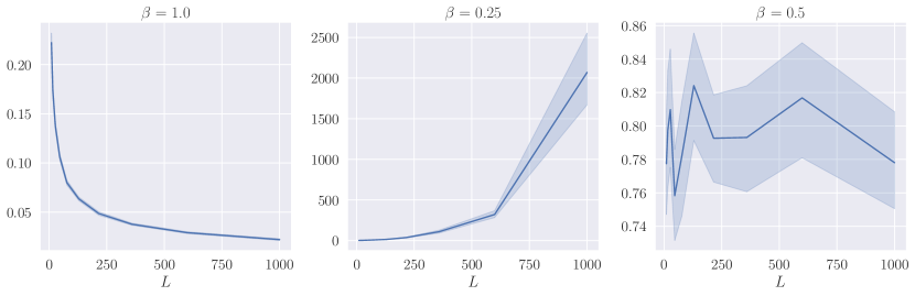
Figure 1: Evolution of $\|h_{L}-h_{0}\|/\|h_{0}\|$ as a function of $L$ for different values of $\beta$ and an i.i.d. $\mathcal{U}(-\sqrt{3/d},\sqrt{3/d})$ initialization of model res-3, with $d=40$. The input is a random Gaussian observation $x$ in dimension $n_{\textnormal{in}}=64$. The experiment is repeated with $50$ independent randomizations.

Corollary 4 highlights three different asymptotic behaviors for $\|h_{L}\|$, depending on the values of $\beta$. For $\beta>\nicefrac{{1}}{{2}}$, statement $(i)$ tells that $h_{L}$ converges towards $h_{0}$ in probability, as $L$ tends to infinity, which means that the neural network is essentially equivalent to an identity mapping. On the other hand, for $\beta<\nicefrac{{1}}{{2}}$, the norm of $h_{L}$ explodes with high probability. Finally, for the critical value $\beta=\nicefrac{{1}}{{2}}$, we see that $h_{L}$ fluctuates around $h_{0}$, with a fluctuation size independent of $L$. Observe that the lower bound in $(iii)$ is not trivial as soon as $\exp(\nicefrac{{3}}{{8}}-\sqrt{\nicefrac{{11}}{{d\delta}}})>1$, i.e., $d>\nicefrac{{99}}{{64\delta}}$. The message of Corollary 4 is that the only scaling leading to a non-degenerate distribution at initialization is for $\beta=\nicefrac{{1}}{{2}}$.

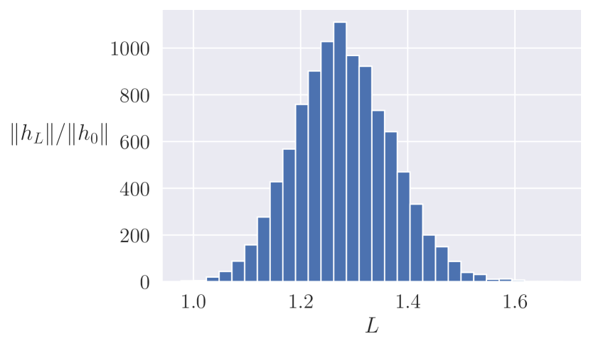
(a) Distribution of $\|h_{L}\|/\|h_{0}\|$

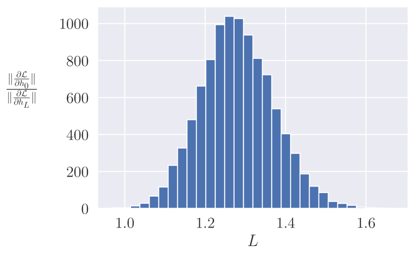
(b) Distribution of $\|\frac{\partial\mathscr{L}}{\partial h_{0}}\|/\|\frac{\partial\mathscr{L}}{\partial h_{L}}\|$

Figure 2: Empirical distributions of the norms for $\beta=\nicefrac{{1}}{{2}}$, $L=10^{3}$, $d=100$. The experiment is repeated with $10^{4}$ independent randomizations.

The three statements of Corollary 4 are illustrated in Figure 1. In this experiment, we consider model res-3, a random Gaussian observation $x$ in dimension $n_{\textnormal{in}}=64$, and parameters initialized with a uniform distribution $\mathcal{U}(-\sqrt{3/d},\sqrt{3/d})$. We refer to Appendix E for a detailed setup of all the experiments of the paper. Figure 2(a) shows the empirical distribution of $\|h_{L}\|/\|h_{0}\|$ when $\beta=\nicefrac{{1}}{{2}}$ for a large number of realizations. This figure illustrates in particular that our bounds are reasonably sharp, since the bounds indicate that the first quartile of the distribution is larger than $0.87$ (whereas the first quartile of the empirical histogram is equal to $1.21$) and the third quartile is less than $2.06$ (whereas the third quartile of the empirical histogram is equal to $1.34$). Determining the exact distribution of $\|h_{L}\|/\|h_{0}\|$ is an interesting avenue for future research that is beyond the scope of the present article. There is however a strong indication that the ratio follows a log-normal distribution, as confirmed by a normality test on (the log of) the empirical distribution.

In a nutshell, the proofs of Propositions 2 and 3 rest upon controlling of the norm of the hidden states, which obeys the recurrence

$$\|h_{k+1}\|^{2}=\|h_{k}\|^{2}+\alpha_{L}^{2}\|V_{k+1}g(h_{k},\theta_{k+1})\|^{2}+2\alpha_{L}\langle h_{k},V_{k+1}g(h_{k},\theta_{k+1})\rangle,$$ (6)

where $\langle\cdot,\cdot\rangle$ denotes the standard scalar product in ${\mathbb{R}}^{d}$. Taking the expectations on both side, one deduces with Assumptions $(A_{1})$ and $(A_{2})$ that

$$\mathbb{E}\big{(}\|V_{k+1}g(h_{k},\theta_{k+1})\|^{2}\big{)} =\mathbb{E}\Big{(}\mathbb{E}\big{(}\|V_{k+1}g(h_{k},\theta_{k+1})\|^{2}\big{)}\,\big{|}\,h_{k},\theta_{k+1}\Big{)}$$

$$=\mathbb{E}\big{(}\|g(h_{k},\theta_{k+1})\|^{2}\big{)}\approx\|h_{k}\|^{2}$$ (7)

and

$$\mathbb{E}\big{(}\langle h_{k},V_{k+1}g(h_{k},\theta_{k+1})\rangle\big{)}=\mathbb{E}\Big{(}\mathbb{E}\big{(}\langle h_{k},V_{k+1}g(h_{k},\theta_{k+1})\rangle\big{|}h_{k},\theta_{k+1}\big{)}\Big{)}=0.$$ (8)

The equalities (2.2) and (8) allow deriving without further work bounds in expectation on $\|h_{L}\|$, as already observed by Arpit et al. (2019). However, the results we are after are stronger since they involve high-probability bounds. A finer control of the deviations of $\|V_{k+1}g(h_{k},\theta_{k+1})\|^{2}$ and $\langle h_{k},V_{k+1}g(h_{k},\theta_{k+1})\rangle$ is then needed. This involves concentration inequalities on random matrices with sub-Gaussian entries.

2.3 Probabilistic bounds on the gradients

Propositions 2 and 3 provide insights on the output of the network when $L$ is large. However, they do not carry information on the backwards dynamics of propagation of the gradients of the loss $p_{k}=\frac{\partial\mathscr{L}}{\partial h_{k}}\in{\mathbb{R}}^{d}$. Assessing the dynamics of the $(p_{k})_{0\leqslant k\leqslant L}$ as a function of $L$ is important since the behavior of this sequence impacts trainability of the network at initialization. Thus, in this subsection, we are interested in quantifying the magnitude of $\|p_{0}-p_{L}\|/\|p_{L}\|$, when $L$ is large. Notice that, contrarily to the previous subsection where we were mostly interested in the last hidden state $h_{L}$, the quantity of interest is now $p_{0}$ (not $p_{L}$), the gradient at index $0$. The reason is that the sequence $(p_{k})_{0\leqslant k\leqslant L}$ is defined backwardly, as we will see below. We also stress that $(p_{k})_{0\leqslant k\leqslant L}$ is the sequence of derivatives of the loss w.r.t. the hidden states $h_{k}$, and not w.r.t. the parameters. The reason for considering this sequence is that the $p_{k}$ are involved in the backpropagation algorithm and are therefore essential for assessing the stability of the gradient descent (see, e.g., Arpit et al., 2019).

Analyzing the behavior of the sequence $(p_{k})_{0\leqslant k\leqslant L}$ is challenging since, according to the backpropagation (or reverse-mode differentiation) formula, one has

$$p_{k}=p_{k+1}+\alpha_{L}\frac{\partial g(h_{k},\theta_{k+1})^{\top}}{\partial h}V_{k+1}^{\top}p_{k+1}.$$

Taking the norm,

$$\|p_{k}\|^{2}=\|p_{k+1}\|^{2}+\alpha_{L}^{2}\Big{\|}\frac{\partial g(h_{k},\theta_{k+1})^{\top}}{\partial h}V_{k+1}^{\top}p_{k+1}\Big{\|}^{2}+2\alpha_{L}\Big{\langle}p_{k+1},\frac{\partial g(h_{k},\theta_{k+1})^{\top}}{\partial h}V_{k+1}^{\top}p_{k+1}\Big{\rangle}.$$

Although the equation looks qualitatively similar to (6), it has the unpleasant feature that $\frac{\partial g(h_{k},\theta_{k+1})}{\partial h}$ depends on $h_{k}$, hence on $\theta_{1},V_{1},\dots,\theta_{k},V_{k}$, while $p_{k+1}$ depends on $\theta_{k+2},V_{k+2},\dots,$ $\theta_{L-1},V_{L-1}$. This forbids applying directly the same proof techniques as for the hidden states. Therefore, to extract useful information from this recurrence equation, one needs to characterize the dependence of the distribution of $\frac{\partial g(h_{k},\theta_{k+1})}{\partial h}$ with respect to $h_{k}$. To do so, it is sometimes assumed that these two quantities are independent (see, e.g., Yang and Schoenholz, 2017). However, assuming independence remains a strong requirement, which is not verified for many network architectures (for example model res-1). We tackle the problem from a different point of view and propose an alternative approach based on forward-mode differentiation, valid under a much weaker assumption. The cost we pay is that we obtain results in expectation and not in high probability.

Let us sketch our approach before stating the results more formally. Let $z\in{\mathbb{R}}^{d}$, and, for any $0\leqslant i,j\leqslant L$, let $\frac{\partial h_{j}}{\partial h_{i}}\in{\mathbb{R}}^{d\times d}$ be the Jacobian matrix of $h_{j}$ with respect to $h_{i}$. Recall that the $(m,n)$-th entry of this matrix equals the derivative of the $m$-th coordinate of $h_{j}$ w.r.t. the $n$-th coordinate of $h_{i}$. Then, letting $q_{k}(z)=\frac{\partial h_{k}}{\partial h_{0}}z$, we have, by the chain rule,

$$q_{k+1}(z)=\frac{\partial h_{k+1}}{\partial h_{k}}q_{k}(z)=q_{k}(z)+\alpha_{L}V_{k+1}\frac{\partial g(h_{k},\theta_{k+1})}{\partial h}q_{k}(z).$$ (9)

Identity (9), which is similar to (4), expresses $q_{k+1}(z)$ as a function of $q_{k}(z)$, and therefore respects the flow of information. Next, assuming that $z$ is random with a Gaussian distribution, it is possible to express one of our quantities of interest, $\|p_{0}\|/\|p_{L}\|$, as a function of the last vector $q_{L}(z)$. Indeed,

$$\frac{\|p_{0}\|^{2}}{\|p_{L}\|^{2}}=\frac{1}{\|p_{L}\|^{2}}\mathbb{E}_{z\sim\mathcal{N}(0,I_{d})}\Big{(}\big{|}p_{0}^{\top}z\big{|}^{2}\Big{)}=\mathbb{E}_{z\sim\mathcal{N}(0,I_{d})}\bigg{(}\Big{|}\Big{(}\frac{p_{L}}{\|p_{L}\|}\Big{)}^{\top}q_{L}(z)\Big{|}^{2}\bigg{)},$$ (10)

where $I_{d}$ is the identity matrix in ${\mathbb{R}}^{d}$ and the second equality is a consequence of

$$p_{0}^{\top}z=\Big{(}\frac{\partial\mathscr{L}}{\partial h_{0}}\Big{)}^{\top}z=\Big{(}\frac{\partial\mathscr{L}}{\partial h_{L}}\Big{)}^{\top}\frac{\partial h_{L}}{\partial h_{0}}z=p_{L}^{\top}q_{L}(z).$$

In summary, the recurrence (9) allows us to derive bounds on the norm of $q_{L}(z)$, which can then transfer to $\|p_{0}\|/\|p_{L}\|$ via (10). For this, it is necessary to make the following assumption on the ratio $p_{L}/\|p_{L}\|$:

• Let $b=p_{L}/\|p_{L}\|$. Then $\mathbb{E}(b|h_{L})=0$ and $\mathbb{E}(b^{\top}b|h_{L})=I_{d}/d$.

It is a mild assumption, which is verified for instance if $n_{\textnormal{out}}=1$ with squared error (for regression) or cross-entropy (for binary classification). In these cases, $p_{L}/\|p_{L}\|=\nicefrac{{B^{\top}}}{{\|B\|_{F}}}$, where $\|\cdot\|_{F}$ is the Frobenius norm and $B$ is the weight matrix of the last layer. We finally need the following assumption, which is the equivalent of Assumption $(A_{2})$ for the gradients.

• One has, almost surely,

  $$\frac{\|q_{k}\|^{2}}{2}\leqslant\mathbb{E}\bigg{(}\Big{\|}\frac{\partial g(h_{k},\theta_{k+1})}{\partial h}q_{k}\Big{\|}^{2}\Big{|}h_{k},q_{k}\bigg{)}\leqslant\|q_{k}\|^{2}.$$

Assumption $(A_{4})$ is satisfied by all the standard architectures listed in Table 1, as shown by the next proposition.

Proposition 5

Let res-1, res-2, and res-3 be the models defined in Table 1. Assume that $(A_{1})$ is satisfied and $\sigma$ is almost everywhere differentiable, with $a\leqslant\sigma^{\prime}\leqslant b$. Then

• Assumption $(A_{4})$ is satisfied for res-1.

• Assumption $(A_{4})$ is satisfied for res-2 and res-3, when the entries of $\sqrt{d}W_{k+1},0\leqslant k\leqslant L-1,$ are symmetric i.i.d. random variables, independent of $d$ and $L$, with unit variance.

The next two propositions are the counterparts of Proposition 2 and Proposition 3 for the gradient dynamics.

Proposition 6

Consider a ResNet (4) such that Assumptions $(A_{1})$-$(A_{4})$ are satisfied. If $L\alpha_{L}^{2}\leqslant 1$, then, for any $\delta\in(0,1)$, with probability at least $1-\delta$,

$$\frac{\|p_{0}-p_{L}\|^{2}}{\|p_{L}\|^{2}}\leqslant\frac{2L\alpha_{L}^{2}}{\delta}.$$

Proposition 7

Consider a ResNet (4) such that Assumptions $(A_{1})$-$(A_{4})$ are satisfied. Then

$$\big{(}1+\frac{1}{2}\alpha_{L}^{2}\big{)}^{L}-1\leqslant\mathbb{E}\bigg{(}\frac{\|p_{0}-p_{L}\|^{2}}{\|p_{L}\|^{2}}\bigg{)}\leqslant(1+\alpha_{L}^{2})^{L}-1.$$

A simple corollary of the propositions above is as follows.

Corollary 8

Consider a ResNet (4) such that Assumptions $(A_{1})$-$(A_{4})$ are satisfied, and take $\alpha_{L}=\nicefrac{{1}}{{L^{\beta}}}$, with $\beta>0$. Then

• If $\beta>\nicefrac{{1}}{{2}}$,

  $$\frac{\|p_{0}-p_{L}\|}{\|p_{L}\|}\xrightarrow[L\rightarrow\infty]{\mathbb{P}}0.$$

• If $\beta<\nicefrac{{1}}{{2}}$,

  $$\mathbb{E}\bigg{(}\frac{\|p_{0}-p_{L}\|^{2}}{\|p_{L}\|^{2}}\bigg{)}\xrightarrow[]{L\rightarrow\infty}\infty.$$

• If $\beta=\nicefrac{{1}}{{2}}$,

  $$\exp\Big{(}\frac{1}{2}\Big{)}-1\leqslant\mathbb{E}\bigg{(}\frac{\|p_{0}-p_{L}\|^{2}}{\|p_{L}\|^{2}}\bigg{)}\leqslant\exp(4)-1.$$

Corollary 8 is illustrated in Figure 3. The experimental protocol is the same as in Figure 1, but we now track $p_{0}$ and $p_{L}$, the gradients of the loss $\mathscr{L}$ with respect to the first and the last hidden states. In accordance with our results, when $\beta>\nicefrac{{1}}{{2}}$, the gradient remains the same from one layer to another (left plot). On the other hand, the middle plot clearly shows that when $\beta<\nicefrac{{1}}{{2}}$ the gradient explodes. Once again, the case $\beta=\nicefrac{{1}}{{2}}$ (right plot) is the only one for which the distribution of gradients at initialization is non-trivial. Figure 2(b) illustrates that the empirical distribution of gradients in this case also seems to be log-normal.

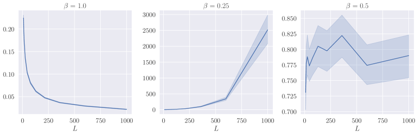
Figure 3: Evolution of $\|p_{0}-p_{L}\|/\|p_{L}\|$ as a function of $L$ for different values of $\beta$ and an i.i.d. $\mathcal{U}(-\sqrt{3/d},\sqrt{3/d})$ initialization of model res-3, with $d=40$. The input is a random Gaussian observation $x$ in dimension $n_{\textnormal{in}}=64$. The experiment is repeated with $50$ independent randomizations.

In summary, this and the previous subsection both point towards the same conclusion: there are three different cases, depending on the value of $\beta$—explosion when $\beta<\nicefrac{{1}}{{2}}$, non-degenerate limit when $\beta=\nicefrac{{1}}{{2}}$, and identity when $\beta>\nicefrac{{1}}{{2}}$. In the explosion case, it is well known that the network cannot be trained (Yang and Schoenholz, 2017). The theory thus points out that the value $\nicefrac{{1}}{{2}}$ plays a pivotal role. Remarkably, this value has a specific interpretation in the continuous-time point of view of ResNets, in terms of SDE. This is the topic that we address in the next section.

3 Scaling in the continuous-time setting

Starting with the discrete ResNet (4), it is tempting to let $L$ go to infinity and consider the network as the discretization of a differential equation where the layer index $k\in\{0,\dots,L\}$ is replaced by the time index $t\in[0,1]$. This interpretation of deep neural networks has been popularized by Chen et al. (2018) and is often referred to as the neural ODE paradigm. Notice that this setting is different from the so-called mean-field analysis, where the width of the network is assumed to be infinite beforehand. In our setting, the width $d$ is assumed to be finite and fixed.

3.1 Convergence towards an SDE in the large-depth regime

One of the main messages of Section 2 is that the standard initialization with i.i.d. parameters leads to a non-degenerate model for large values of $L$ only if $L\alpha_{L}^{2}\approx 1$ (Propositions 2 and 3), or, equivalently, if $\beta=\nicefrac{{1}}{{2}}$ when $\alpha_{L}=\nicefrac{{1}}{{L^{\beta}}}$ (Corollary 4). Remarkably, in the continuous-time limit, this regime corresponds to the discretization of an SDE. Indeed, consider for simplicity the (discrete) ResNet model res-1

$$h_{k+1}=h_{k}+\frac{1}{\sqrt{L}}V_{k+1}\sigma(h_{k}),\quad 0\leqslant k\leqslant L-1,$$ (11)

where the entries of $V_{k+1}$ are assumed to be i.i.d. $\mathcal{N}(0,\nicefrac{{2}}{{d}})$. Recall the following definition:

Definition 9

A one-dimensional Brownian motion $(B_{t})_{t\in[0,1]}$ is a continuous-time stochastic process with $B_{0}=0$, almost surely continuous, with independent increments, and such that for any $0\leqslant s<t\leqslant 1$, $B_{t}-B_{s}\sim\mathcal{N}(0,t-s)$.

Now, let $\mathbf{B}:[0,1]\to{\mathbb{R}}^{d\times d}$ be a $(d\times d)$-dimensional Brownian motion, in the sense that the $(B_{ij})_{1\leqslant i,j\leqslant d}$ are independent one-dimensional Brownian motions. Thus, for any $0\leqslant k\leqslant L-1$ and any $1\leqslant i,j\leqslant d$, we have

$$\mathbf{B}_{\nicefrac{{(k+1)}}{{L}},i,j}-\mathbf{B}_{\nicefrac{{k}}{{L}},i,j}\sim\mathcal{N}\Big{(}0,\frac{1}{L}\Big{)},$$

and the increments for different values of $(i,j,k)$ are independent. As a consequence, the recurrence (11) is equivalent in distribution to the recurrence

$$h_{k+1}^{\top}=h_{k}^{\top}+\sqrt{\frac{2}{d}}\sigma(h_{k}^{\top})(\mathbf{B}_{\nicefrac{{(k+1)}}{{L}}}-\mathbf{B}_{\nicefrac{{k}}{{L}}}),\quad 0\leqslant k\leqslant L-1.$$

(Note that this is true because $V_{k+1}$ has the same distribution as $V_{k+1}^{\top}$.) We recognize the Euler-Maruyama discretization (Kloeden and Platen, 1992) on the $\{k/L,0\leqslant k\leqslant L\}$ mesh of the SDE

$$dH_{t}^{\top}=\sqrt{\frac{2}{d}}\sigma(H_{t}^{\top})d\mathbf{B}_{t},\quad t\in[0,1],$$ (12)

where the output of the network is now a function of the final value of $H$, that is, $H_{1}$. The link between the discrete ResNet (11) and the SDE (12) is formalized in the next proposition.

Proposition 10

Consider the res-1 model, where the entries of $V_{k+1}$ are i.i.d. Gaussian $\mathcal{N}(0,\nicefrac{{2}}{{d}})$ random variables. Assume that the activation function $\sigma$ is Lipschitz continuous. Then the SDE (12) has a unique solution $H$ and, for any $0\leqslant k\leqslant L$,

$${\mathbb{E}}\big{(}\|H_{\nicefrac{{k}}{{L}}}-h_{k}\|\big{)}\leqslant\frac{c}{\sqrt{L}},$$

for some $c>0$.

Notice that the requirement that $\sigma$ is Lipschitz continuous is satisfied by most classical activation functions, including ReLU. This proposition is interesting for several reasons. First, the scaling $\beta=\nicefrac{{1}}{{2}}$, which is exactly the one that yields a non-trivial dynamics at initialization, corresponds in the continuous world to a remarkably ‘simple’ model of diffusion. This shows that very deep neural networks properly initialized with i.i.d. weights are equivalent to solutions of SDE. This analogy opens interesting perspectives for training deep networks using automatic differentiation for solutions of neural SDE (Li et al., 2020).

Second, we stress that the emergence of an SDE instead of an ODE carries an important message. Several authors (including, e.g., Thorpe and van Gennip, 2018) have shown that, under appropriate assumptions, a deep ResNet converges in the large depth limit to an ODE and not an SDE. The reason why we obtain an SDE here is intrinsically connected with the choice of i.i.d. initialization for the weights, which makes a Brownian motion appear at the limit, as highlighted above. In other words, the i.i.d. initialization, the choice $\beta=\nicefrac{{1}}{{2}}$ (the relevant critical value exhibited in Section 2), and the emergence of an SDE are intimately linked together. On the other hand, the case $\beta=1$ matches with an ODE if the initialization is not i.i.d., as we will see in Subsection 3.2.

Finally, we point out that Proposition 10 states the convergence of a ResNet towards an SDE for the basic architecture res-1 and for Gaussian initialization. The extension to more general settings is an interesting direction of research, although clearly beyond the scope of the present paper (see, e.g., Peluchetti and Favaro, 2020, and Cohen et al., 2021, for results in this direction).

3.2 Scaling in the neural ODE setting

Convergence towards an ODE.

The basic message of our Proposition 10 is that an i.i.d. initialization, together with $\beta=\nicefrac{{1}}{{2}}$, leads to an SDE rather than an ODE. A natural question is then whether a different choice of weight distributions (at initialization) and scaling can lead to a classical neural ODE.

To answer this question and leave the world of i.i.d. initialization, we assume that the weights $(V_{k})_{1\leqslant k\leqslant L}$ and $(\theta_{k})_{1\leqslant k\leqslant L}$ are discretizations of smooth functions $\mathscr{V}:[0,1]\rightarrow{\mathbb{R}}^{d\times d}$ and $\Theta:[0,1]\rightarrow{\mathbb{R}}^{p}$. We then consider the general iteration (4) with $\alpha_{L}=\nicefrac{{1}}{{L}}$, that is,

$$\begin{split}h_{0}&=Ax,\quad h_{k+1}=h_{k}+\frac{1}{L}V_{k+1}g(h_{k},\theta_{k+1}),\quad 0\leqslant k\leqslant L-1,\end{split}$$ (13)

where $V_{k}=\mathscr{V}_{k/L}$ and $\theta_{k}=\Theta_{k/L}$. Of course, it is still possible to consider $(V_{k})_{1\leqslant k\leqslant L}$ (resp. $(\theta_{k})_{1\leqslant k\leqslant L}$) as random variables, by letting $(\mathscr{V}_{t})_{t\in[0,1]}$ (resp. $(\Theta_{t})_{t\in[0,1]}$) be a continuous-time stochastic process. In this model, we shall need the following assumption:

• For any $0\leqslant k\leqslant L-1$, one has $V_{k}=\mathscr{V}_{k/L}$ and $\theta_{k}=\Theta_{k/L}$, where the stochastic processes $\mathscr{V}$ and $\Theta$ are almost surely Lipschitz continuous and bounded.

More precisely, almost surely, there exist $K_{\mathscr{V}},K_{\Theta},C_{\mathscr{V}},C_{\Theta}>0$, such that, for any $s,t\in[0,1]$,

$$\|\mathscr{V}_{t}-\mathscr{V}_{s}\|\leqslant K_{\mathscr{V}}|t-s|, \quad\|\Theta_{t}-\Theta_{s}\|\leqslant K_{\Theta}|t-s|,\quad\|\mathscr{V}_{t}\|\leqslant C_{\mathscr{V}},\quad\|\Theta_{t}\|\leqslant C_{\Theta}.$$

A typical model that satisfies Assumption $(A_{5})$ is obtained by letting the entries of $\mathscr{V}$ and $\Theta$ be independent Gaussian processes with expectation zero and squared exponential covariance $K(x,x^{\prime})=\exp(-\frac{(x-x^{\prime})^{2}}{2\ell^{2}})$, where $\ell>0$.

We shall also need the following requirement on $g$, which is satisfied by all our models as soon as $\sigma$ is Lipschitz continuous:

• The function $g$ is Lipschitz continuous on compact sets, in the sense that for any compact $\mathscr{P}\subseteq{\mathbb{R}}^{p}$, there exists $K_{\mathscr{P}}>0$ such that, for all $h,h^{\prime}\in{\mathbb{R}}^{d}$, $\theta\in\mathscr{P}$,

  $$\|g(h,\theta)-g(h^{\prime},\theta)\|\leqslant K_{\mathscr{P}}\|h-h^{\prime}\|,$$

  and for any compact $\mathscr{D}\subseteq{\mathbb{R}}^{d}$, there exists $K_{\mathscr{D},\mathscr{P}}>0$ such that, for all $h\in\mathscr{D}$, $\theta,\theta^{\prime}\in\mathscr{P}$,

  $$\|g(h,\theta)-g(h,\theta^{\prime})\|\leqslant K_{\mathscr{D},\mathscr{P}}\|\theta-\theta^{\prime}\|.$$

Under Assumptions $(A_{5})$ and $(A_{6})$, the recurrence (13) almost surely converges towards the neural ODE given by

$$\begin{split}H_{0}&=Ax,\quad dH_{t}=\mathscr{V}_{t}g(H_{t},\Theta_{t})dt,\quad t\in[0,1],\end{split}$$ (14)

as shown by the proposition below.

Proposition 11

Consider model (13) such that Assumptions $(A_{5})$ and $(A_{6})$ are satisfied. Then the ODE (14) has a unique solution $H$, and, almost surely, there exists some $c>0$ such that, for any $0\leqslant k\leqslant L$,

$$\|H_{\nicefrac{{k}}{{L}}}-h_{k}\|\leqslant\frac{c}{L}.$$

It should be stressed that the transition from the discrete recurrence (13) to the continuous-time differential equation (14) relies on the assumptions that the weight sequences $(\theta_{k})_{1\leqslant k\leqslant L}$ and $(V_{k})_{1\leqslant k\leqslant L}$ are the discretizations of smooth limiting processes $\Theta$ and $\mathscr{V}$ on the one hand, and that the scaling $\alpha_{L}$ is chosen as $\nicefrac{{1}}{{L}}$ on the other hand. From a practical perspective, Proposition 11 shows that it is possible to initialize ResNets in the ODE regime, by choosing a smooth stochastic process, discretizing it at each layer, and taking a $\nicefrac{{1}}{{L}}$ scaling. This is in sharp contrast with the results of Sections 2 and 3.1, which show that the usual i.i.d. procedure leads to a neural SDE.

Stability and scaling.

Assuming that the weights of the network are discretizations of a smooth function (Assumption $(A_{5})$), it is possible to obtain stability results, depending on the value of $\beta$, similarly to what has been done in Section 2. We show below that $\beta=1$ is a critical value, by examining the hidden states, in the same way as $\beta=\nicefrac{{1}}{{2}}$ is a critical value in the i.i.d. setting. Similar results can be shown for the gradients. We begin by a proposition handling the cases $\beta>1$ and $\beta=1$.

Proposition 12

Consider a ResNet (4) such that Assumptions $(A_{5})$ and $(A_{6})$ are satisfied. Let $\alpha_{L}=\nicefrac{{1}}{{L^{\beta}}}$, with $\beta>0$.

• If $\beta>1$, then, almost surely,

  $$\frac{\|h_{L}-h_{0}\|}{\|h_{0}\|}\xrightarrow[]{L\rightarrow\infty}0.$$

• If $\beta=1$, then, almost surely, there exists some $c>0$ such that

  $$\frac{\|h_{L}-h_{0}\|}{\|h_{0}\|}\leqslant c.$$

The explosion case ($\beta<1$) is more delicate to deal with. We prove it for a linear model, and leave for future work the extension to more general cases.

Proposition 13

Consider the res-1 model, taking $\sigma$ as the identity function. Assume that Assumption $(A_{5})$ is satisfied and that $\mathscr{V}_{0}^{T}$ has a positive eigenvalue. Let $\alpha_{L}=\nicefrac{{1}}{{L^{\beta}}}$, with $\beta\in(0,1)$. Then, almost surely,

$$\max_{k}\frac{\|h_{k}-h_{0}\|}{\|h_{0}\|}\xrightarrow[]{L\rightarrow\infty}\infty.$$

The assumption of the existence of a positive eigenvalue for $\mathscr{V}_{0}^{\top}$ is mild. For instance, if the entries of $\mathscr{V}_{0}$ are i.i.d. random variables with finite moments of all order, Götze and Jalowy (2021) show that such an eigenvalue exists with probability at least $1-\nicefrac{{1}}{{d}}$ for $d$ large enough.

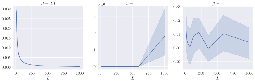
Figure 4: Evolution of $\|h_{L}-h_{0}\|/\|h_{0}\|$ as a function of $L$ for different values of $\beta$ and a smooth initialization of model res-3, with $d=40$. The input is a random Gaussian observation $x$ in dimension $n_{\textnormal{in}}=64$. The experiment is repeated with $50$ independent randomizations.

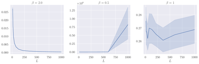
Figure 5: Evolution of $\|p_{0}-p_{L}\|/\|p_{L}\|$ as a function of $L$ for different values of $\beta$ and a smooth initialization of model res-3, with $d=40$. The input is a random Gaussian observation $x$ in dimension $n_{\textnormal{in}}=64$. The experiment is repeated with $50$ independent randomizations.

In this setting, we observe experimentally a behavior of the output and of the gradients when $L$ grows large similar to the one explored in Section 2. This is illustrated in Figures 4 and 5, which mirror Figures 1 and 3 in Section 2. The figures clearly show that there exist three cases for the output and for the gradients: an identity case (left plots), an explosion case (middle), and a non-trivial case separating explosion and identity (right). However, the remarkable point is that the separation occurs for $\beta=1$, and not $\beta=\nicefrac{{1}}{{2}}$, as predicted by Propositions 12 and 13.

4 Experiments

We experimentally investigate in this section two questions. The first one is to know whether there exists a range of scaling factors $\beta>0$ and weight initializations, beyond the i.i.d. and the smooth regimes. The second question is whether our analysis, which pertains to the initialization phase, provides insights into the training phase, beyond initialization.

4.1 Intermediate regimes

In order to describe the transition between the i.i.d. and smooth cases, a possible route is to consider that the weights are increments of a $\gamma$-Hölder stochastic process. This model is interesting insofar as the Brownian motion (SDE regime) is $(\nicefrac{{1}}{{2}}-\varepsilon)$-Hölder ($\varepsilon>0$) and a Lipschitz continuous stochastic process (ODE regime) is $1$-Hölder.

In line with the above, in a series of experiments, we initialize the weights as increments of a fractional Brownian motion $(B^{H}_{t})_{t\in[0,1]}$. Recall that $B^{H}$ is a continuous-time Gaussian process, starting at zero, with zero expectation for all $t\in[0,1]$, and covariance function

$$\mathbb{E}(B^{H}_{s}B^{H}_{t})=\frac{1}{2}(|s|^{2H}+|t|^{2H}-|t-s|^{2H}),\quad 0\leqslant s,t\leqslant 1,$$

where $H\in(0,1)$ is called the Hurst index. This index describes the raggedness of the process, with a higher value leading to a smoother process. When $H=\nicefrac{{1}}{{2}}$, the process is a standard Brownian motion (Definition 9), whose increments are independent by construction. When $H>\nicefrac{{1}}{{2}}$, the increments of the process are positively correlated, while if $H<\nicefrac{{1}}{{2}}$ the increments are negatively correlated. Importantly, a fractional Brownian motion with Hurst index $H$ is $(H-\varepsilon)$-Hölder continuous for any $\varepsilon>0$. In the limit when $H\rightarrow 1$, the trajectories converge to linear functions (whose increments satisfy $(A_{5})$). As an illustration, Figure 6 depicts three realizations of a fractional Brownian motion with $H=0.2$ (left), $H=0.5$ (middle), and $H=0.8$ (right).

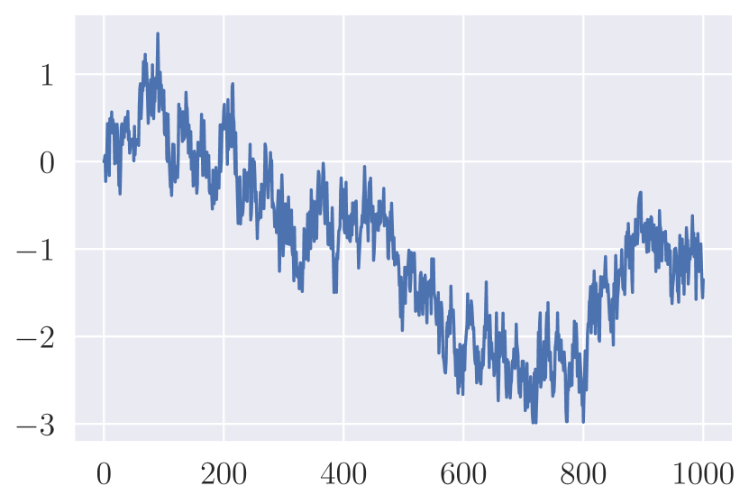
(a) $H=0.2$

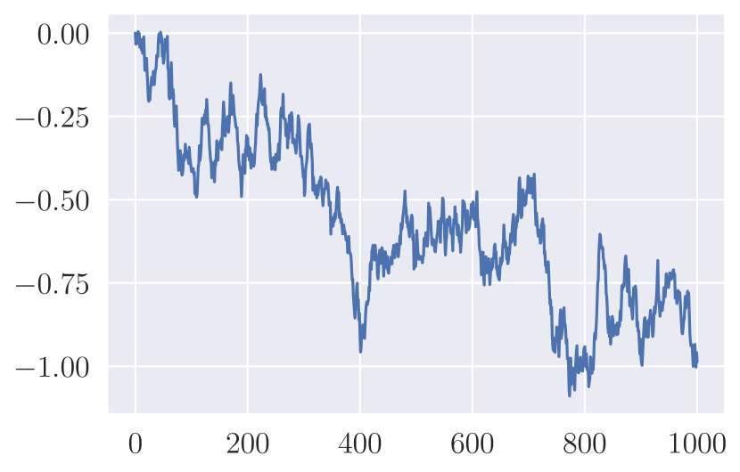
(b) $H=0.5$

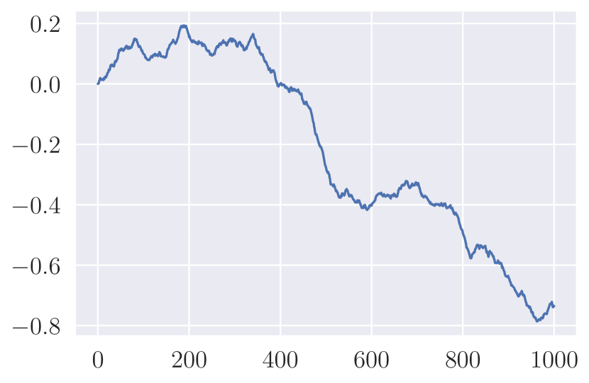
(c) $H=0.8$

Figure 6: Examples of realizations of a fractional Brownian motion $B^{H}$ for different Hurst indexes $H$. Note that the smaller the value of $H$, the more irregular the trajectory is.

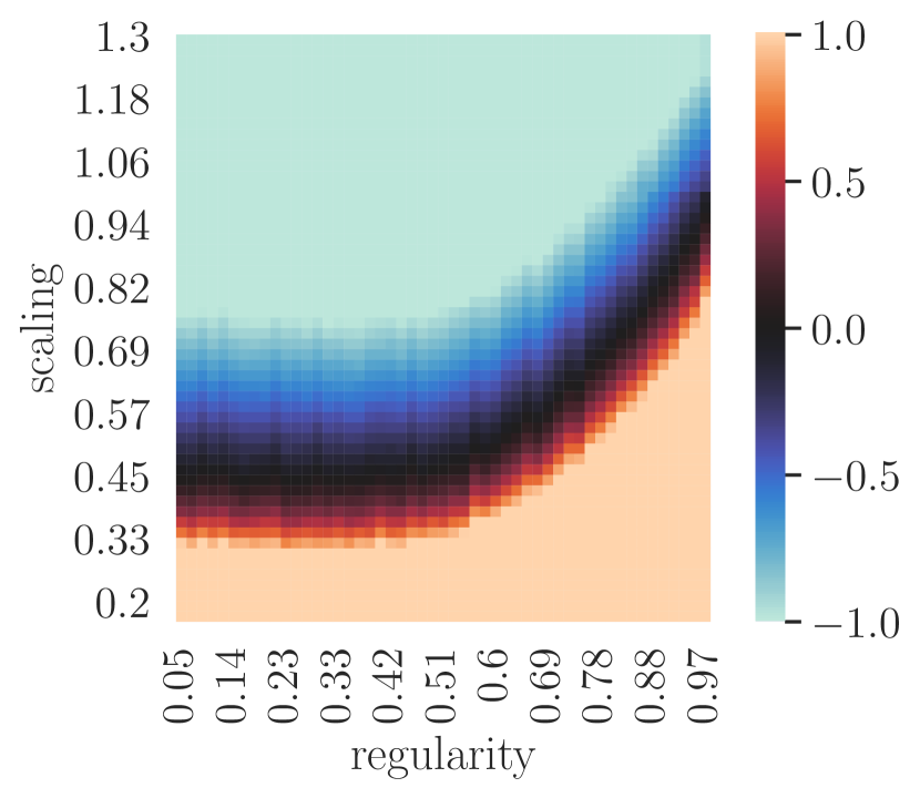
(a) $\ln_{10}(\|h_{L}-h_{0}\|/\|h_{0}\|)$

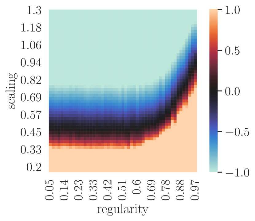
(b) $\ln_{10}(\|p_{0}-p_{L}\|/\|p_{L}\|)$

Figure 7: Magnitude of the outputs and of the gradients as a function of the regularity of the weights (Hurst index $H$) and of the scaling factor $\beta$. The orange zone corresponds to the explosion regime, i.e., $\|h_{L}-h_{0}\|\gg\|h_{0}\|$ and $\|p_{0}-p_{L}\|\gg\|p_{L}\|$. The blue zone corresponds to the identity regime, i.e., $\|h_{L}-h_{0}\|\ll\|h_{0}\|$ and $\|p_{0}-p_{L}\|\ll\|p_{L}\|$. Finally, the black zone is an intermediate regime, where $\|h_{L}-h_{0}\|\approx\|h_{0}\|$ and $\|p_{0}-p_{L}\|\approx\|p_{L}\|$.

In order to assess the effect of the scaling factor $\beta$ and the Hurst index $H$, we initialize a neural network res-3 with $d=40$, $L=1000$, various values of $\beta\in[0.2,1.3]$, and with weights taken as increments of fractional Brownian motions with various Hurst indices $H\in(0,1)$. Figure 7 depicts the empirical magnitude of the output and the gradients at initialization as a function of the Hurst index $H$ and the scaling factor $\beta$. First note that we recover the two regimes (i.i.d. and smooth) discussed so far. For $H=\nicefrac{{1}}{{2}}$, the i.i.d. regime kicks in, with explosion ($\beta<\nicefrac{{1}}{{2}}$, orange zone), non-trivial behavior ($\beta=\nicefrac{{1}}{{2}}$, black zone), and identity ($\beta>\nicefrac{{1}}{{2}}$, blue zone). Likewise, we see at $H=1$ a similar pattern in the smooth regime, with, as predicted by Proposition 12, a critical value $\beta=1$. Beyond these two specific cases, we observe for an index $H$ varying in $(\nicefrac{{1}}{{2}},1)$ a whole range of intermediate situations, where the transition between identity and explosion seems to happen for a critical $\beta=H$. Interestingly, for $H<\nicefrac{{1}}{{2}}$, the transition seems to saturate at the value $\beta=\nicefrac{{1}}{{2}}$.

The take-home message is that the choice of the scaling of a ResNet seems to be closely linked to the regularity of the weights as a function of the layer. More precisely, for all regimes, the critical scaling factor between explosion and identity seems to have a natural interpretation as the (Hölder) regularity of the underlying continuous-time stochastic process. We believe that the mathematical understanding of this connection, beyond the fractional Brownian motion case, is a promising research direction for the future. Finally, these experiments suggest that it is sensible to initialize a ResNet for any value of the scaling $\beta\in(\nicefrac{{1}}{{2}},1)$, while avoiding the identity and explosion situations, by simulating a fractional Brownian motion of Hurst index $H=\beta$ and initializing the weights as the increments of this process.

4.2 Beyond initialization

At initialization, before the gradient descent, the distribution of the weights $(\theta_{k})_{1\leqslant k\leqslant L}$ and $(V_{k})_{1\leqslant k\leqslant L}$ is chosen by the practitioner. By contrast, during and after training, control is lost on these distributions, making the picture more complex. In particular, the existence and characterization of a continuous-time stochastic process whose discretization matches the trained ResNet is an interesting but difficult problem. Attacking this question requires a fine understanding of the interaction between training dynamics and the regularity of the sequence of the weights during the gradient descent. However, there is experimental evidence that the trained weights exhibit strong structure as a function of the layer index $k$ (Cohen et al., 2021; Bayer et al., 2022), and that their regularity strongly depends on the choice of initialization. Figure 8 depicts this mechanism by plotting a given coordinate of $\theta_{k}$ as a function of the layer index $k$ ranging from $1$ to the depth $L=1000$, after training.

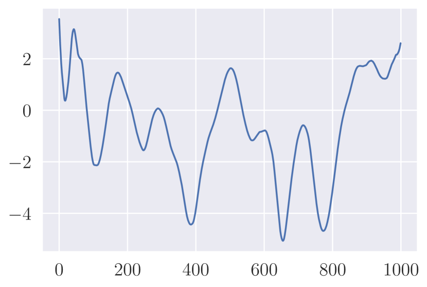
(a) $\beta=1$, smooth initialization

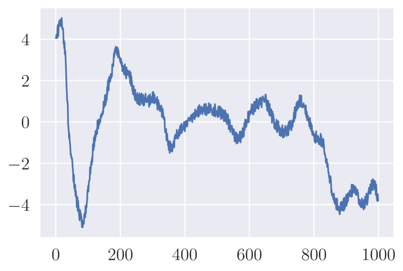
(b) $\beta=1$, i.i.d. initialization

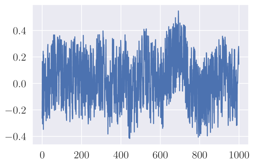
(c) $\beta=\nicefrac{{1}}{{2}}$, i.i.d. initialization

Figure 8: Plot of a given coordinate of $\theta_{k}$, after training, as a function of the layer index $k$ ranging from $1$ to the depth $L=1000$ for three different choices of $\beta$ and initializations.

To investigate the link between regularity of the weights at initialization, scaling, and performance after training, we train ResNets on the datasets MNIST (Deng, 2012) and CIFAR-10 (Krizhevsky, 2009). As in Subsection 4.1, we initialize the ResNets with various scaling factors and weights that are increments of fractional Brownian motions with different regularities. Then, for each combination of weight initialization and scaling factor, the ResNet is trained using the Adam optimizer (Kingma and Ba, 2015) for $10$ epochs. The results in terms of accuracy are presented in Figure 9 (light orange = good performance, blue = bad performance). We observe a pattern similar to the one of Figure 7, however shifted downwards. This means that, for a given regularity, the network is unable to learn if it is initialized with a scaling too far below the critical value, which of course is connected with the gradient explosion issue discussed previously. On the other hand, and perhaps more surprisingly, the performance seems to be more or less stable in the identity region, with perhaps a small degradation in the case of CIFAR-10. This somewhat contrasts with the results from Yang and Schoenholz (2017), who exhibit a decrease in performance for i.i.d. initialization and a large scaling factor $\beta$. Note however that, in our experiments, we adapted the learning rate of the gradient descent on a grid by cross-validation. This was done to prevent a slowdown in training when the scaling factor $\beta$ is too large, since, in the gradient descent, the gradients updates are also scaled by the factor $\nicefrac{{1}}{{L^{\beta}}}$—which gets smaller as $\beta$ increases. The interplay between the learning rate and the scaling factor is one of the keys to better assess how the performance of the trained network is connected with the scaling.

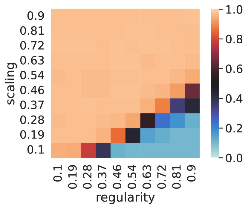
(a) On MNIST

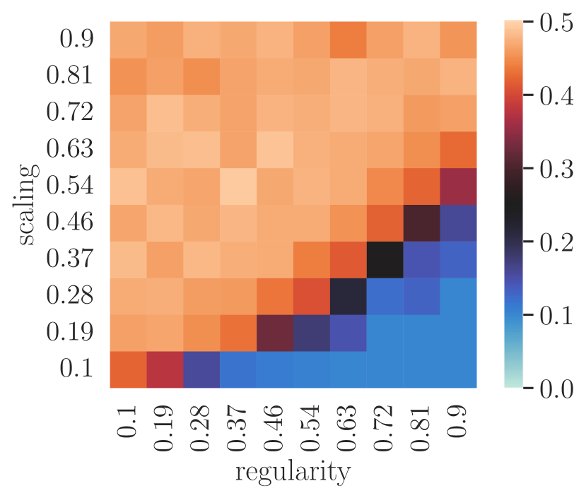
(b) On CIFAR-10

Figure 9: Accuracy after training as a function of the regularity of the weights at initialization and scaling. For each point of the heatmap, the model was trained on a grid of learning rates, and the best performance is shown.

Acknowledgments

The authors thank S. Schoenholz for fruitful discussion. P. Marion has been supported by a grant from Région Île-de-France and by a Google PhD Fellowship award.

Appendix A Proofs

Throughout the proofs, the $i$-th coordinate of a vector $v$ is denoted by $v_{i}$. Similarly, the $i$-th row of a matrix $M$ is denoted by $M_{i}$, and its $(i,j)$-th entry by $M_{ij}$.

A.1 Proof of Proposition 1

Statement $(i)$ is clear (with $C=1$) since, for any $h\in{\mathbb{R}}^{d}$,

$$\|\sigma(h)\|^{2}\in\big{[}a^{2}\|h\|^{2},b^{2}\|h\|^{2}\big{]}\subseteq\big{[}\frac{1}{2}\|h\|^{2},\|h\|^{2}\big{]}.$$

With respect to statement $(ii)$, it is enough to show that for any $h\in{\mathbb{R}}^{d}$ and any random matrix $W$ satisfying the assumptions of the proposition, one has

$$\frac{\|h\|^{2}}{2}\leqslant\mathbb{E}\big{(}\|\sigma(Wh)\|^{2}\big{)}\leqslant\|h\|^{2}\quad\textnormal{and}\quad\mathbb{E}\big{(}\|\sigma(Wh)\|^{8}\big{)}\leqslant C\|h\|^{8},$$

as well as

$$\mathbb{E}\big{(}\|\operatorname*{ReLU}(Wh)\|^{2}\big{)}=\frac{\|h\|^{2}}{2}\quad\textnormal{and}\quad\mathbb{E}\big{(}\|\operatorname*{ReLU}(Wh)\|^{8}\big{)}\leqslant C\|h\|^{8}.$$

The two claims with the squared norms are consequences of Lemmas 16 and 17 in Appendix B, together with the fact that the variance of the entries of $W$ equals $1/d$. In order to prove the other two statements, first note that $\mathbb{E}(\|\sigma(Wh)\|^{8})\leqslant\mathbb{E}(\|Wh\|^{8})$ and $\mathbb{E}(\|\operatorname*{ReLU}(Wh)\|^{8})\leqslant\mathbb{E}(\|Wh\|^{8})$. The results are then consequences of Lemma 21 in Appendix C, which states that

$$\mathbb{E}\left(\frac{\|Wh\|^{8}}{\|h\|^{8}}\right)\leqslant 1+\frac{384s^{4}}{d}+\frac{3072s^{6}}{d^{2}}\leqslant 1+384s^{4}+3072s^{6}.$$

A.2 Proof of Proposition 2

According to Lemma 14 below, one has

$$\mathbb{E}\Big{(}\frac{\|h_{L}-h_{0}\|^{2}}{\|h_{0}\|^{2}}\Big{)}\leqslant\big{(}\big{(}1+\alpha_{L}^{2}\big{)}^{L}-1\big{)}.$$

But, for $L\alpha_{L}^{2}\leqslant 1$, we have $(1+\alpha_{L}^{2})^{L}-1\leqslant\exp(L\alpha_{L}^{2})-1\leqslant 2L\alpha_{L}^{2}.$ Therefore,

$$\mathbb{E}\Big{(}\frac{\|h_{L}-h_{0}\|^{2}}{\|h_{0}\|^{2}}\Big{)}\leqslant 2L\alpha_{L}^{2},$$

and the result follows from Markov’s inequality.

Lemma 14

Consider a ResNet (4) such that Assumptions $(A_{1})$ and $(A_{2})$ are satisfied. Then

$$\bigg{(}\Big{(}1+\frac{\alpha_{L}^{2}}{2}\Big{)}^{L}-1\bigg{)}\leqslant\mathbb{E}\Big{(}\frac{\|h_{L}-h_{0}\|^{2}}{\|h_{0}\|^{2}}\Big{)}\leqslant\Big{(}\big{(}1+\alpha_{L}^{2}\big{)}^{L}-1\Big{)}.$$

Proof (Lemma 14)

Taking the squared norm of the forward update rule (4) and dividing by $\|h_{0}\|^{2}$ yields

$$\frac{\|h_{k+1}\|^{2}}{\|h_{0}\|^{2}}=\frac{1}{\|h_{0}\|^{2}}\Big{(}\|h_{k}\|^{2}+\alpha_{L}^{2}\|V_{k+1}g(h_{k},\theta_{k+1})\|^{2}+2\alpha_{L}\langle h_{k},V_{k+1}g(h_{k},\theta_{k+1})\rangle\Big{)}.$$ (15)

We deduce by Assumptions $(A_{1})$ and $(A_{2})$ that

$$\Big{(}1+\frac{\alpha_{L}^{2}}{2}\Big{)}\mathbb{E}\Big{(}\frac{\|h_{k}\|^{2}}{\|h_{0}\|^{2}}\Big{)}\leqslant\mathbb{E}\Big{(}\frac{\|h_{k+1}\|^{2}}{\|h_{0}\|^{2}}\Big{)}\leqslant(1+\alpha_{L}^{2})\mathbb{E}\Big{(}\frac{\|h_{k}\|^{2}}{\|h_{0}\|^{2}}\Big{)}.$$

Therefore, by recurrence, we are led to

$$\Big{(}1+\frac{\alpha_{L}^{2}}{2}\Big{)}^{k}\leqslant\mathbb{E}\Big{(}\frac{\|h_{k}\|^{2}}{\|h_{0}\|^{2}}\Big{)}\leqslant(1+\alpha_{L}^{2})^{k}.$$ (16)

Now, observe that $h_{L}=h_{0}+\alpha_{L}\sum_{k=0}^{L-1}V_{k+1}g(h_{k},\theta_{k+1})$. Thus, we have

$$\mathbb{E}\Big{(}\frac{\|h_{L}-h_{0}\|^{2}}{\|h_{0}\|^{2}}\Big{)}=\alpha_{L}^{2}\sum_{k,k^{\prime}=0}^{L-1}\mathbb{E}\Big{(}\frac{g(h_{k},\theta_{k+1})^{\top}V_{k+1}^{\top}V_{k^{\prime}+1}g(h_{k^{\prime}},\theta_{k^{\prime}+1})}{\|h_{0}\|^{2}}\Big{)}.$$

By conditioning on all random variables except $V_{k^{\prime}+1}$ for $k<k^{\prime}$ (and $V_{k+1}$ for $k>k^{\prime}$), it is easy to see that the only non-zero terms are when $k=k^{\prime}$. This yields

$$\mathbb{E}\Big{(}\frac{\|h_{L}-h_{0}\|^{2}}{\|h_{0}\|^{2}}\Big{)} =\alpha_{L}^{2}\sum_{k=0}^{L-1}\mathbb{E}\Big{(}\frac{\|V_{k+1}g(h_{k},\theta_{k+1})\|^{2}}{\|h_{0}\|^{2}}\Big{)}$$

$$\leqslant\alpha_{L}^{2}\sum_{k=0}^{L-1}\mathbb{E}\Big{(}\frac{\|h_{k}\|^{2}}{\|h_{0}\|^{2}}\Big{)}$$

(by Assumptions $$A_{1} A_{2}$$ and )

$$\leqslant\alpha_{L}^{2}\sum_{k=0}^{L-1}(1+\alpha_{L}^{2})^{k}$$

(by (16))

$$=\big{(}\big{(}1+\alpha_{L}^{2}\big{)}^{L}-1\big{)}.$$

Similarly,

$$\mathbb{E}\Big{(}\frac{\|h_{L}-h_{0}\|^{2}}{\|h_{0}\|^{2}}\Big{)} \geqslant\frac{\alpha_{L}^{2}}{2}\sum_{k=0}^{L-1}\mathbb{E}\Big{(}\frac{\|h_{k}\|^{2}}{\|h_{0}\|^{2}}\Big{)}$$

$$=\Big{(}\Big{(}1+\frac{\alpha_{L}^{2}}{2}\Big{)}^{L}-1\Big{)}.$$

 

A.3 Proof of Proposition 3

Dividing (15) by $\|h_{k}\|^{2}$ and taking the logarithm leads to

$$\ln(\|h_{k+1}\|^{2})=\ln(\|h_{k}\|^{2})+\ln\bigg{(}1+\alpha_{L}^{2}\frac{\|V_{k+1}g(h_{k},\theta_{k+1})\|^{2}}{\|h_{k}\|^{2}}+2\alpha_{L}\Big{\langle}\frac{h_{k}}{\|h_{k}\|},\frac{V_{k+1}g(h_{k},\theta_{k+1})}{\|h_{k}\|}\Big{\rangle}\bigg{)}.$$

Let

$$Y_{k,1}=\alpha_{L}^{2}\frac{\|V_{k+1}g(h_{k},\theta_{k+1})\|^{2}}{\|h_{k}\|^{2}},\quad Y_{k,2}=2\alpha_{L}\Big{\langle}\frac{h_{k}}{\|h_{k}\|},\frac{V_{k+1}g(h_{k},\theta_{k+1})}{\|h_{k}\|}\Big{\rangle},$$

and $Y_{k}=Y_{k,1}+Y_{k,2}$. The proof of Proposition 3 strongly relies on the following lemma, which provides technical information on the moments of $Y_{k,1}$ and $Y_{k,2}$. For the sake of clarity, its proof is postponed to Appendix B.

Lemma 15

Assume that Assumptions $(A_{1})$ and $(A_{2})$ are satisfied. Then

$\mathbb{E}(Y_{k,2}|h_{k})=0$. $(E_{2})$ $\frac{\alpha_{L}^{2}}{2}\leqslant\mathbb{E}(Y_{k,1}|h_{k})\leqslant\alpha_{L}^{2}$. $(E_{3})$ $\mathbb{E}(Y_{k,1}Y_{k,2}|h_{k})=0$. $(E_{4})$ $\mathbb{E}(Y_{k,2}^{2}|h_{k})\leqslant 4\frac{\alpha_{L}^{2}}{d}$.

$\mathbb{E}(Y_{k,2}^{4}|h_{k})\leqslant 2048\frac{s^{4}\alpha_{L}^{4}}{d^{2}}$. $(E_{6})$ $\mathbb{E}(Y_{k,1}^{4}|h_{k})\leqslant C\left(3072\frac{s^{6}}{d^{2}}+384\frac{s^{4}}{d}+1\right)\alpha_{L}^{8}$. $(E_{7})$ $\mathbb{E}(Y_{k,1}^{2}|h_{k})\leqslant\sqrt{C}\left(128\frac{s^{4}}{d}+1\right)\alpha_{L}^{4}$.

For $c>0$, we have

$$\mathbb{P}\Big{(}\frac{\|h_{L}\|^{2}}{\|h_{0}\|^{2}}\geqslant c\Big{)} =\mathbb{P}\Big{(}\ln(\|h_{L}\|^{2})-\ln(\|h_{0}\|^{2})\geqslant\ln(c)\Big{)}$$

$$=\mathbb{P}\Big{(}\sum_{k=0}^{L-1}\ln(1+Y_{k})\geqslant\ln(c)\Big{)}$$

$$\leqslant\mathbb{P}\Big{(}\sum_{k=0}^{L-1}Y_{k}\geqslant\ln(c)\Big{)}$$

(using $$\ln(1+x)\leqslant x x>-1$$ for ).

Let $S=\sum_{k=0}^{L-1}Y_{k}-\mathbb{E}(Y_{k}|h_{k})$. By $(E_{1})$ and $(E_{2})$,

$$\sum_{k=0}^{L-1}\mathbb{E}(Y_{k}|h_{k})\leqslant L\alpha_{L}^{2}.$$

So, for $c>\exp(L\alpha_{L}^{2})$,

$$\mathbb{P}\Big{(}\frac{\|h_{L}\|^{2}}{\|h_{0}\|^{2}}\geqslant c\Big{)} \leqslant\mathbb{P}\bigg{(}S\geqslant\ln(c)-\sum_{k=0}^{L-1}\mathbb{E}(Y_{k}|h_{k})\bigg{)}$$

$$\leqslant\mathbb{P}(S\geqslant\ln(c)-L\alpha_{L}^{2})$$

$$\leqslant\mathbb{P}\Big{(}S^{2}\geqslant\big{(}\ln(c)-L\alpha_{L}^{2}\big{)}^{2}\Big{)}$$

$$\leqslant\frac{\mathbb{E}(S^{2})}{(\ln(c)-L\alpha_{L}^{2})^{2}}$$ (17)

(by Markov’s inequality.)

It remains to upper bound $\mathbb{E}(S^{2})$. To this aim, note that

$$\mathbb{E}(S^{2})=\sum_{k=0}^{L-1}\mathbb{E}\Big{(}\big{(}Y_{k}-\mathbb{E}(Y_{k}|h_{k})\big{)}^{2}\Big{)} \leqslant\sum_{k=0}^{L-1}\mathbb{E}\big{(}Y_{k}^{2}\big{)}$$

$$\leqslant 4\frac{L\alpha_{L}^{2}}{d}+128\sqrt{C}\frac{L\alpha_{L}^{4}s^{4}}{d}+\sqrt{C}L\alpha_{L}^{4}$$

(by $$(E_{3}) (E_{4}) (E_{7})$$, , and )

$$\leqslant 5\frac{L\alpha_{L}^{2}}{d}.$$

The last inequality is true for $\alpha_{L}^{2}\leqslant\frac{1}{\sqrt{C}(d+128s^{4})}$. Therefore, by inequality (17), we obtain, for $c>\exp(L\alpha_{L}^{2})$,

$$\mathbb{P}\Big{(}\frac{\|h_{L}\|^{2}}{\|h_{0}\|^{2}}\geqslant c\Big{)}\leqslant\frac{5L\alpha_{L}^{2}}{d\left(\ln(c)-L\alpha_{L}^{2}\right)^{2}}.$$

We conclude that, for any $\delta\in(0,1)$, with probability at least $1-\delta$,

$$\frac{\|h_{L}\|^{2}}{\|h_{0}\|^{2}}<\exp\left(L\alpha_{L}^{2}+\sqrt{\frac{5L\alpha_{L}^{2}}{d\delta}}\right).$$

This shows statement $(ii)$ of the proposition.

Next, to prove statement $(i)$, observe that $c>0$,

$$\mathbb{P}\Big{(}\frac{\|h_{L}\|^{2}}{\|h_{0}\|^{2}}\leqslant c\Big{)} =\mathbb{P}\Big{(}\ln(\|h_{L}\|^{2})-\ln(\|h_{0}\|^{2})\leqslant\ln(c)\Big{)}$$

$$=\mathbb{P}\Big{(}\sum_{k=0}^{L-1}\ln(1+Y_{k})\leqslant\ln(c)\Big{)}$$

$$=\mathbb{P}\Big{(}\sum_{k=0}^{L-1}\ln(1+Y_{k})\leqslant\ln(c)\text{ and }\forall k,Y_{k}\geqslant-\frac{1}{2}\Big{)}$$

$$\quad+\mathbb{P}\Big{(}\sum_{k=0}^{L-1}\ln(1+Y_{k})\leqslant\ln(c)\text{ and }\exists k,Y_{k}<-\frac{1}{2}\Big{)}.$$

Using the inequality $\ln(1+x)\geqslant x-x^{2}$ for $x\geqslant-\nicefrac{{1}}{{2}}$, we obtain

$$\mathbb{P}\Big{(}\frac{\|h_{L}\|^{2}}{\|h_{0}\|^{2}}\leqslant c\Big{)} \leqslant\mathbb{P}\Big{(}\sum_{k=0}^{L-1}Y_{k}-Y_{k}^{2}\leqslant\ln(c)\text{ and }\forall k,Y_{k}\geqslant-\frac{1}{2}\Big{)}$$

$$\quad+\mathbb{P}\Big{(}\sum_{k=0}^{L-1}\ln(1+Y_{k})\leqslant\ln(c)\text{ and }\exists k,Y_{k}<-\frac{1}{2}\Big{)}.$$

Thus,

$$\mathbb{P}\Big{(}\frac{\|h_{L}\|^{2}}{\|h_{0}\|^{2}}\leqslant c\Big{)}\leqslant\mathbb{P}\Big{(}\sum_{k=0}^{L-1}Y_{k}-Y_{k}^{2}\leqslant\ln(c)\Big{)}+\sum_{k=0}^{L-1}\mathbb{P}\Big{(}Y_{k,2}<-\frac{1}{2}\Big{)}.$$ (18)

We handle the two terms above on the right-hand side separately. For the first term, let $Z_{k}=Y_{k}-Y_{k}^{2}$ and $S=\sum_{k=0}^{L-1}Z_{k}-\mathbb{E}(Z_{k}|h_{k})$. Observe that, by $(E_{1})$-$(E_{4})$ and $(E_{7})$,

$$\sum_{k=0}^{L-1}\mathbb{E}(Z_{k}|h_{k})\geqslant\frac{L\alpha_{L}^{2}}{2}-4\frac{L\alpha_{L}^{2}}{d}-128\sqrt{C}\frac{L\alpha_{L}^{4}s^{4}}{d}-\sqrt{C}L\alpha_{L}^{4}\geqslant\frac{3}{8}L\alpha_{L}^{2},$$ (19)

where the last inequality is valid for $d\geqslant 64$ and $\alpha_{L}^{2}\leqslant\frac{1}{16\sqrt{C}(2s^{4}+1)}$. Hence, for $0<c<\exp(\nicefrac{{3L\alpha_{L}^{2}}}{{8}})$,

$$\mathbb{P}\bigg{(}\sum_{k=0}^{L-1}Y_{k}-Y_{k}^{2}\leqslant\ln c\bigg{)} =\mathbb{P}\Big{(}S\leqslant\ln(c)-\sum_{k=0}^{L-1}\mathbb{E}(Z_{k}|h_{k})\Big{)}$$

$$\leqslant\mathbb{P}\Big{(}S\leqslant\ln(c)-\frac{3L\alpha_{L}^{2}}{8}\Big{)}$$

$$\leqslant\mathbb{P}\Big{(}S^{2}\geqslant\Big{(}\ln(c)-\frac{3L\alpha_{L}^{2}}{8}\Big{)}^{2}\Big{)}$$

$$\leqslant\frac{\mathbb{E}(S^{2})}{\big{(}\ln(c)-\frac{3L\alpha_{L}^{2}}{8}\big{)}^{2}}$$

(by Markov’s inequality.)

Using the $c_{r}$-inequality $(a+b)^{n}\leqslant 2^{n-1}(a^{n}+b^{n})$ respectively for $n=2$ and $n=4$, we see that

$$\mathbb{E}(S^{2}) =\sum_{k=0}^{L-1}\mathbb{E}\Big{(}\big{(}Z_{k}-\mathbb{E}(Z_{k}|h_{k})\big{)}^{2}\Big{)}\leqslant\sum_{k=0}^{L-1}\mathbb{E}\big{(}Z_{k}^{2}\big{)}\leqslant 2\sum_{k=0}^{L-1}\mathbb{E}\big{(}Y_{k}^{2}\big{)}+\mathbb{E}\big{(}Y_{k}^{4}\big{)}$$

$$\leqslant 2\sum_{k=0}^{L-1}\mathbb{E}(Y_{k,1}^{2})+\mathbb{E}(Y_{k,2}^{2})+2\mathbb{E}(Y_{k,1}Y_{k,2})+8\mathbb{E}(Y_{k,1}^{4})+8\mathbb{E}(Y_{k,2}^{4}).$$

By $(E_{3})$-$(E_{7})$, it is easy to verify that, for $d\geqslant 64$ and $\alpha_{L}^{2}\leqslant\frac{1}{(\sqrt{C}s^{4}/16+2\sqrt{C}+8s^{4})d}$,

$$\mathbb{E}(S^{2}) \leqslant 10\frac{L\alpha_{L}^{2}}{d}.$$

This shows that, for $c<\exp(\nicefrac{{3L\alpha_{L}^{2}}}{{8}})$,

$$\mathbb{P}\Big{(}\sum_{k=0}^{L-1}Y_{k}-Y_{k}^{2}\leqslant\ln(c)\Big{)}\leqslant\frac{10L\alpha_{L}^{2}}{d\big{(}\ln(c)-\frac{3L\alpha_{L}^{2}}{8}\big{)}^{2}}.$$

To conclude the proof, it remains to upper bound the second term of inequality (18). According to inequality (22) in the proof of Lemma 15 (with $t=\nicefrac{{1}}{{2}}$), one has

$$\sum_{k=0}^{L-1}\mathbb{P}\Big{(}Y_{k,2}<-\frac{1}{2}\Big{)}\leqslant 2L\exp\Big{(}-\frac{d}{64\alpha_{L}^{2}s^{2}}\Big{)}.$$

Putting everything together, we are led to

$$\mathbb{P}\Big{(}\frac{\|h_{L}\|^{2}}{\|h_{0}\|^{2}}\leqslant c\Big{)}\leqslant\frac{10L\alpha_{L}^{2}}{d\big{(}\ln(c)-\frac{3L\alpha_{L}^{2}}{8}\big{)}^{2}}+2L\exp\Big{(}-\frac{d}{64\alpha_{L}^{2}s^{2}}\Big{)}.$$

Take $\delta\in(0,1)$. Then, if $2L\exp\big{(}-\frac{d}{64\alpha_{L}^{2}s^{2}}\big{)}\leqslant\frac{\delta}{11}$, with probability at least $1-\delta$,

$$\frac{\|h_{L}\|^{2}}{\|h_{0}\|^{2}}>\exp\bigg{(}\frac{3L\alpha_{L}^{2}}{8}-\sqrt{\frac{11L\alpha_{L}^{2}}{d\delta}}\bigg{)}.$$

Notice that this inequality is valid under the assumption $\alpha_{L}^{2}\leqslant\frac{2}{(\sqrt{C}s^{4}+4\sqrt{C}+16s^{4})d}$.

A.4 Proof of Corollary 4

Statement $(i)$ is a consequence of Proposition 2, whereas $(ii)$ is a consequence of Proposition 3 $(i)$. The latter is valid under the conditions $d\geqslant 64$ and $\alpha_{L}\leqslant\frac{2}{(\sqrt{C}s^{4}+4\sqrt{C}+16s^{4})d}$, which is automatically satisfied for all $L$ large enough. Furthermore, an inspection of the proof of Proposition 3 reveals that the divergence in high probability of $\|h_{L}\|$ can be proved under the relaxed assumption $d\geqslant 9$. Indeed, the main constraint on $d$ comes from the lower bound (19), where one needs to make sure that $\frac{L\alpha_{L}^{2}}{2}-4\frac{L\alpha_{L}^{2}}{d}>0$, which is the case for $d=9$.

To prove $(iii)$, we use a union bound on both statements of Proposition 3.

A.5 Proof of Proposition 5

The first claim follows from the observation that

$$\frac{\partial g(h_{k},\theta_{k+1})}{\partial h}q_{k}=\begin{pmatrix}\sigma^{\prime}(h_{k,1})&0&\dots&0\\ 0&\sigma^{\prime}(h_{k,2})&\dots&0\\ \vdots&\vdots&\ddots&\vdots\\ 0&0&\dots&\sigma^{\prime}(h_{k,d})\\ \end{pmatrix}q_{k},$$

from $(A_{1})$, and from the assumption on $\sigma^{\prime}$.

Let us now prove $(ii)$. In the rest of the proof, the subscript $k$ is ignored to lighten the notation. Observe that

$$\frac{\partial g(h,\theta)}{\partial h}q=V\begin{pmatrix}\sigma^{\prime}(\langle W_{1},h\rangle)&0&\dots&0\\ 0&\sigma^{\prime}(\langle W_{2},h\rangle)&\dots&0\\ \vdots&\vdots&\ddots&\vdots\\ 0&0&\dots&\sigma^{\prime}(\langle W_{d},h\rangle)\\ \end{pmatrix}Wq.$$

Denote by $D$ the matrix in the middle of the right-hand side. Then

$$\mathbb{E}\bigg{(}\Big{\|}\frac{\partial g(h,\theta)}{\partial h}q\Big{\|}^{2}\Big{|}h,q\bigg{)}=\mathbb{E}\big{(}\|VDWq\|^{2}|h,q\big{)} =\mathbb{E}\big{(}\|DWq\|^{2}|h,q\big{)}$$

(by $$(A_{1})$$)

For model res-2, we have

$$\mathbb{E}\bigg{(}\Big{\|}\frac{\partial g(h,\theta)}{\partial h}q\Big{\|}^{2}\Big{|}h,q\bigg{)}=\mathbb{E}\bigg{(}\sum_{i=1}^{d}\Big{(}\sum_{j=1}^{d}W_{ij}q_{j}\Big{)}^{2}\sigma^{\prime}(\langle W_{i},h\rangle)\bigg{|}h,q\bigg{)}.$$

The conclusion follows from the hypothesis that $a\leqslant\sigma^{\prime}\leqslant b$ and $\mathbb{E}\big{(}\|Wq\|^{2}|q\big{)}=\|q\|^{2}$. For model res-3, we have

$$\mathbb{E}\bigg{(}\Big{\|}\frac{\partial g(h,\theta)}{\partial h}q\Big{\|}^{2}\Big{|}h,q\bigg{)}=\mathbb{E}\bigg{(}\sum_{i=1}^{d}\Big{(}\sum_{j=1}^{d}W_{ij}q_{j}\Big{)}^{2}\mathbf{1}_{\sum_{j=1}^{d}W_{ij}h_{j}\geqslant 0}\bigg{|}h,q\bigg{)}.$$

Since the $(W_{ij})_{1\leqslant i,j\leqslant d}$ are symmetric random variables, we conclude that

$$\mathbb{E}\bigg{(}\Big{\|}\frac{\partial g(h,\theta)}{\partial h}q\Big{\|}^{2}\Big{|}h,q\bigg{)}=\frac{1}{2}\mathbb{E}\bigg{(}\sum_{i=1}^{d}\Big{(}\sum_{j=1}^{d}W_{ij}q_{j}\Big{)}^{2}\bigg{|}q\bigg{)}=\frac{1}{2}\mathbb{E}\big{(}\|Wq\|^{2}|q\big{)}=\frac{\|q\|^{2}}{2}.$$

A.6 Proof of Proposition 6

Letting $b=p_{L}/\|p_{L}\|$, as in Assumption $(A_{3})$, and taking expectation in (10), we obtain

$$\mathbb{E}\bigg{(}\frac{\|p_{0}\|^{2}}{\|p_{L}\|^{2}}\bigg{)}=\mathbb{E}(|b^{\top}q_{L}(z)|^{2}) =\frac{1}{d}\mathbb{E}(\|q_{L}(z)\|^{2})$$ (20)

$$\quad\mbox{(by $(A_{3})$)}.$$

The rest of the proof is similar to the proof of Proposition 2. From (9), we have

$$\|q_{k+1}(z)\|^{2}=\|q_{k}(z)\|^{2}+\alpha_{L}^{2}\Big{\|}V_{k+1}\frac{\partial g(h_{k},\theta_{k+1})}{\partial h}q_{k}(z)\Big{\|}^{2}+2\alpha_{L}\Big{\langle}q_{k}(z),V_{k+1}\frac{\partial g(h_{k},\theta_{k+1})}{\partial h}q_{k}(z)\Big{\rangle}.$$

By independence of $V_{k+1}$ from $q_{k}(z)$ and $\frac{\partial g(h_{k},\theta_{k+1})}{\partial h}$,

$$\mathbb{E}\Big{(}\Big{\langle}q_{k}(z),V_{k+1}\frac{\partial g(h_{k},\theta_{k+1})}{\partial h}q_{k}(z)\Big{\rangle}\Big{)}=0.$$

Next,

$$\mathbb{E}\Big{(}\Big{\|}V_{k+1}\frac{\partial g(h_{k},\theta_{k+1})}{\partial h}q_{k}(z)\Big{\|}^{2}\Big{)} =\mathbb{E}\bigg{(}\mathbb{E}\Big{(}\Big{\|}V_{k+1}\frac{\partial g(h_{k},\theta_{k+1})}{\partial h}q_{k}(z)\Big{\|}^{2}\Big{|}h_{k},\theta_{k+1},q_{k}(z)\Big{)}\bigg{)}$$

$$=\mathbb{E}\left(\Big{\|}\frac{\partial g(h_{k},\theta_{k+1})}{\partial h}q_{k}(z)\Big{\|}^{2}\right)$$

(by $$(A_{1})$$)

$$=\mathbb{E}\left(\mathbb{E}\left(\Big{\|}\frac{\partial g(h_{k},\theta_{k+1})}{\partial h}q_{k}(z)\Big{\|}^{2}\Big{|}h_{k},q_{k}(z)\right)\right).$$

By Assumption $(A_{3})$, we are led to

$$\big{(}1+\frac{1}{2}\alpha_{L}^{2}\big{)}\mathbb{E}(\|q_{k}(z)\|^{2})\leqslant\mathbb{E}(\|q_{k+1}(z)\|^{2})\leqslant(1+\alpha_{L}^{2})\mathbb{E}(\|q_{k}(z)\|^{2}),$$

and thus, by induction, since $q_{0}(z)=z$ and $\mathbb{E}(\|z\|^{2})=d$,

$$d\big{(}1+\frac{1}{2}\alpha_{L}^{2}\big{)}^{k}\leqslant\mathbb{E}(\|q_{k}(z)\|^{2})\leqslant d(1+4\alpha_{L}^{2})^{k}.$$

In particular, for $k=L$,

$$d\big{(}1+\frac{1}{2}\alpha_{L}^{2}\big{)}^{L}\leqslant\mathbb{E}(\|q_{L}(z)\|^{2})\leqslant d(1+\alpha_{L}^{2})^{L}.$$

Therefore, by (20),

$$\big{(}1+\frac{1}{2}\alpha_{L}^{2}\big{)}^{L}\leqslant\mathbb{E}\bigg{(}\frac{\|p_{0}\|^{2}}{\|p_{L}\|^{2}}\bigg{)}\leqslant(1+\alpha_{L}^{2})^{L}.$$

To finish the proof, observe that

$$\frac{1}{\|p_{L}\|}(p_{0}-p_{L})^{\top}z=b^{\top}(q_{L}(z)-z).$$

Using arguments similar to (20), we may write

$$\mathbb{E}\bigg{(}\frac{\|p_{0}-p_{L}\|^{2}}{\|p_{L}\|^{2}}\bigg{)}=\frac{1}{d}\mathbb{E}\Big{(}\frac{\|q_{L}(z)-z\|^{2}}{\|z\|^{2}}\Big{)}.$$

Now, upon noting that $q_{L}(z)-z=q_{L}(z)-q_{0}(z)=\alpha_{L}\sum_{k=0}^{L-1}V_{k+1}\frac{\partial g(h_{k},\theta_{k+1})}{\partial h}q_{k}(z)$,

$$\mathbb{E}(\|q_{L}(z)-z\|^{2}) =\alpha_{L}^{2}\sum_{k,k^{\prime}=0}^{L-1}\mathbb{E}\left(q_{k}(z)^{\top}\frac{\partial g(h_{k},\theta_{k+1})^{\top}}{\partial h}V_{k+1}^{\top}V_{k^{\prime}+1}\frac{\partial g(h_{k}^{\prime},\theta_{k^{\prime}+1})}{\partial h}q_{k^{\prime}}(z)\right)$$

$$=\alpha_{L}^{2}\sum_{k=0}^{L-1}\mathbb{E}\left(\bigg{\|}V_{k+1}\frac{\partial g(h_{k},\theta_{k+1})}{\partial h}q_{k}(z)\bigg{\|}^{2}\right)$$

$$\leqslant d\alpha_{L}^{2}\sum_{k=0}^{L-1}(1+\alpha_{L}^{2})^{k}$$

$$=d\big{(}(1+\alpha_{L}^{2})^{L}-1\big{)}\leqslant d\big{(}\exp(L\alpha_{L}^{2})-1\big{)}\leqslant 2dL\alpha_{L}^{2},$$

for $L\alpha_{L}^{2}\leqslant 1$. Note that the second equality is obtained by conditioning on every random variable except $V_{k^{\prime}+1}$ for $k<k^{\prime}$ (and $V_{k+1}$ for $k>k^{\prime}$). Finally, by using Markov’s inequality, we conclude that, for any $\varepsilon>0$,

$$\mathbb{P}\big{(}\|p_{0}-p_{L}\|^{2}\geqslant\varepsilon\|p_{L}\|^{2}\big{)}\leqslant\frac{2L\alpha_{L}^{2}}{\varepsilon}.$$

A.7 Proof of Proposition 7

The proof of Proposition 6 reveals that

$$\mathbb{E}\bigg{(}\frac{\|p_{0}-p_{L}\|^{2}}{\|p_{L}\|^{2}}\bigg{)}\leqslant(1+\alpha_{L}^{2})^{L}-1.$$

Using similar arguments, one has

$$\mathbb{E}\bigg{(}\frac{\|p_{0}-p_{L}\|^{2}}{\|p_{L}\|^{2}}\bigg{)}=\frac{1}{d}\mathbb{E}\Big{(}\frac{\|q_{L}(z)-z\|^{2}}{\|z\|^{2}}\Big{)}\geqslant\alpha_{L}^{2}\sum_{k=0}^{L-1}\big{(}1+\frac{1}{2}\alpha_{L}^{2}\big{)}^{k}=\big{(}1+\frac{1}{2}\alpha_{L}^{2}\big{)}^{L}-1.$$

A.8 Proof of Corollary 8

The first statement is an immediate consequence of Proposition 6. The second one is a consequence of Proposition 7 and the fact that, for $\beta<1$,

$$\Big{(}1+\frac{1}{L^{\beta}}\Big{)}^{L}=\exp\Big{(}L\ln\Big{(}1+\frac{1}{L^{\beta}}\Big{)}\Big{)}\sim\exp\big{(}L^{1-\beta}\big{)}\rightarrow\infty.$$

Finally, $(iii)$ follows from Proposition 7.

A.9 Proof of Proposition 10

The proposition is a consequence of Kloeden and Platen (1992, Theorems 4.5.3 and 10.2.2) for the SDE

$$dH_{t}^{\top}=\sqrt{\frac{d}{2}}\sigma(H_{t}^{\top})dB_{t}.$$

Letting $a(h,t)=0$ and $b(h,t)=\sqrt{\frac{d}{2}}\sigma(h)$, we need to check the following assumptions:

• The functions $a(\cdot,\cdot)$ and $b(\cdot,\cdot)$ are jointly measurable on ${\mathbb{R}}^{d}\times[0,1]$.

• There exists a constant $C_{1}>0$ such that, for any $x,y\in{\mathbb{R}}^{d}$, $t\in[0,1]$,

  $$\|a(x,t)-a(y,t)\|+\|b(x,t)-b(y,t)\|\leqslant C_{1}\|x-y\|.$$

• There exists a constant $C_{2}>0$ such that, for any $x\in{\mathbb{R}}^{d}$, $t\in[0,1]$,

  $$\|a(x,t)\|+\|b(x,t)\|\leqslant C_{2}(1+\|x\|).$$

• ${\mathbb{E}}\big{(}|H_{0}\|^{2}\big{)}<\infty$.

• There exists a constant $C_{3}>0$ such that, for any $x\in{\mathbb{R}}^{d}$, $s,t\in[0,1]$,

  $$\|a(x,t)-a(x,s)\|+\|b(x,t)-b(x,s)\|\leqslant C_{3}(1+\|x\|)|t-s|^{\nicefrac{{1}}{{2}}}.$$

Assumptions $(H_{1})$, $(H_{4})$, and $(H_{5})$ readily follow from the definitions. Assumption $(H_{2})$ is true since $\sigma$ is Lipschitz continuous, and $(H_{3})$ follows from

$$\|\sigma(x)\|\leqslant b\|x\|\leqslant\|x\|\leqslant 1+\|x\|.$$

A.10 Proof of Proposition 11

Let $\psi:{\mathbb{R}}^{d}\times[0,1]\to{\mathbb{R}}^{d}$ be defined for any $h\in{\mathbb{R}}^{d}$, $t\in[0,1]$, by $\psi(h,t)=\mathscr{V}_{t}g(h,\Theta_{t})$. With this notation, the ODE (14) is equivalent to the initial value problem

$$dH_{t}=\psi(H_{t},t)dt,\quad H_{0}=Ax.$$

By Assumptions $(A_{5})$ and $(A_{6})$, $\psi$ is Lipschitz continuous in its first argument, in the sense that there exists $K>0$ such that, for all $h,h^{\prime}\in{\mathbb{R}}^{d},t\in[0,1]$,

$$\|\psi(h,t)-\psi(h^{\prime},t)\|\leqslant K\|h-h^{\prime}\|.$$

In addition, it is continuous in its second one. Thus, according to the Picard-Lindelöf theorem (Theorem 22 in Appendix D), this is enough to show that the neural ODE (14) has a unique solution on $[0,1]$. Note that the solution $H$ is continuous on $[0,1]$ and is therefore bounded by a constant $M>0$.

In order to prove the approximation bound of Proposition 11, we start by proving that both $\psi$ and $H$ are Lipschitz continuous in $t$. Under $(A_{5})$ and $(A_{6})$, this is clear for $\psi$ since $H$ is bounded. Moreover, for any $[s,t]\subset[0,1]$, we have

$$\|H_{t}-H_{s}\|=\Big{\|}\int_{s}^{t}\psi(H_{u},u)du\Big{\|} \leqslant\int_{s}^{t}\|\psi(H_{u},u)\|du$$

$$\leqslant(t-s)\sup_{\begin{subarray}{c}u\in[0,1]\\ h\in{\mathbb{R}}^{d},\|h\|\leqslant M\end{subarray}}\|\psi(h,u)\|.$$

Now, let $K_{1}$ and $K_{2}$ denote the Lipschitz constants of $\psi$ (in both arguments) and $H$ respectively, and, for any $0\leqslant k\leqslant L$, let $t_{k}=\nicefrac{{k}}{{L}}$. Then we have, for $k\geqslant 1$,

$$\|H_{t_{k}}-h_{k}\|$$

$$\quad=\big{\|}H_{t_{k-1}}+\int_{t_{k-1}}^{t_{k}}\psi(H_{u},u)du-h_{k-1}-\frac{1}{L}\psi(h_{k-1},t_{k-1})\big{\|}$$

$$\quad\leqslant\|H_{t_{k-1}}-h_{k-1}\|+\int_{t_{k-1}}^{t_{k}}\|\psi(H_{u},u)-\psi(h_{k-1},t_{k-1})\|du$$

$$\quad\leqslant\|H_{t_{k-1}}-h_{k-1}\|+K_{1}\int_{t_{k-1}}^{t_{k}}\|H_{u}-h_{k-1}\|du+K_{1}\int_{t_{k-1}}^{t_{k}}|u-t_{k-1}|du$$

$$\quad\leqslant\Big{(}1+\frac{K_{1}}{L}\Big{)}\|H_{t_{k-1}}-h_{k-1}\|+K_{1}\int_{t_{k-1}}^{t_{k}}\|H_{u}-H_{t_{k-1}}\|du+K_{1}\int_{t_{k-1}}^{t_{k}}|u-t_{k-1}|du$$

$$\quad\leqslant\Big{(}1+\frac{K_{1}}{L}\Big{)}\|H_{t_{k-1}}-h_{k-1}\|+(K_{2}+1)K_{1}\int_{t_{k-1}}^{t_{k}}|u-t_{k-1}|du$$

$$\quad=\Big{(}1+\frac{K_{1}}{L}\Big{)}\|H_{t_{k-1}}-h_{k-1}\|+\frac{(K_{2}+1)K_{1}}{2L^{2}}.$$

By recurrence, we obtain

$$\|H_{t_{k}}-h_{k}\| \leqslant\sum_{j=0}^{k-1}\Big{(}1+\frac{K_{1}}{L}\Big{)}^{j}\times\frac{(K_{2}+1)K_{1}}{2L^{2}}\leqslant L\Big{(}1+\frac{K_{1}}{L}\Big{)}^{L}\times\frac{(K_{2}+1)K_{1}}{2L^{2}}$$

$$\leqslant e^{K_{1}}\frac{(K_{2}+1)K_{1}}{2L},$$

which concludes the proof.

A.11 Proof of Proposition 12

Starting from (4) and using Assumption $(A_{6})$, one easily obtains the existence of $C_{1}$ and $C_{2}$ (whose values depend on the realization of $\mathscr{V}$ and $\Theta$) such that

$$\|h_{k+1}\|\leqslant(1+C_{1}\alpha_{L})\|h_{k}\|+C_{2}\alpha_{L}.$$

By recurrence,

$$\|h_{k+1}\|\leqslant(1+C_{1}\alpha_{L})^{k}\Big{(}\|h_{0}\|+\frac{C_{2}}{C_{1}}\Big{)}.$$

Hence, using $\alpha_{L}\leqslant\nicefrac{{1}}{{L}}$,

$$\|h_{k+1}\|\leqslant\exp(C_{1})\Big{(}\|h_{0}\|+\frac{C_{2}}{C_{1}}\Big{)}.$$

Since $g$ is Lipschitz continuous on compact sets, it is bounded on every ball of ${\mathbb{R}}^{d}\times{\mathbb{R}}^{p}$. The result is then a consequence of the identity

$$h_{L}-h_{0}=\alpha_{L}\sum_{k=0}^{L-1}V_{k+1}g(h_{k},\theta_{k+1}),$$

since we showed that each term in the sum is bounded by some constant $C_{3}>0$, independent of $L$ and $k$. Hence we have that

$$\|h_{L}-h_{0}\|\leqslant C_{3}L\alpha_{L}=C_{3}L^{1-\beta},$$

yielding the results depending on the value of $\beta$.

A.12 Proof of Proposition 13

In the linear case, (4) can be written

$$h_{k+1}=h_{k}+\alpha_{L}V_{k+1}h_{k},\quad 0\leqslant k\leqslant L-1.$$

Take $y$ a unit-norm eigenvector of $\mathscr{V}_{0}^{\top}$ with associated eigenvalue $\lambda>0$. Then

$$\langle h_{k+1},y\rangle =\langle h_{k}+\alpha_{L}V_{k+1}h_{k},y\rangle$$

$$=\langle h_{k},y\rangle+\alpha_{L}\langle h_{k},V_{k+1}^{\top}y\rangle$$

$$=\langle h_{k},y\rangle+\lambda\alpha_{L}\langle h_{k},y\rangle+\alpha_{L}\langle h_{k},(V_{k+1}-\mathscr{V}_{0})^{\top}y\rangle.$$

Since $\mathscr{V}$ is Lipschitz and $V_{k+1}=\mathscr{V}_{k+1/L}$, there exists $c$ such that $\|V_{k+1}-\mathscr{V}_{0}\|\leqslant c\frac{k+1}{L}$. Hence

$$|\langle h_{k+1},y\rangle|\geqslant(1+\lambda\alpha_{L})|\langle h_{k},y\rangle|-c\alpha_{L}\frac{k+1}{L}\|h_{k}\|.$$

Then, by recurrence,

$$|\langle h_{L},y\rangle| \geqslant(1+\lambda\alpha_{L})^{L}|\langle h_{0},y\rangle|-c\frac{\alpha_{L}}{L}\sum_{k=0}^{L-1}(k+1)(1+\lambda\alpha_{L})^{k}\|h_{k}\|$$

$$\geqslant(1+\lambda\alpha_{L})^{L}|\langle h_{0},y\rangle|-c\alpha_{L}(1+\lambda\alpha_{L})^{L}\max_{k}\|h_{k}\|.$$

Let $M=\frac{|\langle h_{0},y\rangle|}{2c\alpha_{L}}$, and suppose that $\|h_{k}\|\leqslant M$ for all $0\leqslant k\leqslant L$. Then

$$\|h_{L}\| \geqslant|\langle h_{L},y\rangle|$$

(by the Cauchy-Schwartz inequality)

$$\geqslant(1+\lambda\alpha_{L})^{L}\big{(}|\langle h_{0},y\rangle|-cM\alpha_{L}\big{)}.$$

Then, for $\lambda\alpha_{L}\leqslant 1$,

$$\|h_{L}\|\geqslant\frac{1}{2}(1+\lambda\alpha_{L})^{L}|\langle h_{0},y\rangle|\geqslant\frac{1}{2}\exp\big{(}\frac{\lambda L\alpha_{L}}{2}\big{)}|\langle h_{0},y\rangle|.$$

Thus, since $L\alpha_{L}=L^{1-\beta}$, we have that $\|h_{L}\|\rightarrow\infty$, which contradicts our assumption that $\|h_{k}\|\leqslant M$ for all $0\leqslant k\leqslant L$. We deduce that, for all $L$ large enough,

$$\max_{k}\|h_{k}\|>\frac{|\langle h_{0},y\rangle|}{2c\alpha_{L}}\xrightarrow[]{L\rightarrow\infty}\infty.$$

Furthermore,

$$\max_{k}\frac{\|h_{k}-h_{0}\|}{\|h_{0}\|}>\frac{|\langle h_{0},y\rangle|}{2c\|h_{0}\|\alpha_{L}}-1\xrightarrow[]{L\rightarrow\infty}\infty.$$

Appendix B Technical results

B.1 Lemmas 16 and 17

Lemma 16

Let $W\in{\mathbb{R}}^{d\times d}$ be a matrix whose entries are symmetric i.i.d. random variables, with finite variance, and let $\sigma$ be an activation function such that, for all $x\in{\mathbb{R}},a|x|\leqslant|\sigma(x)|\leqslant b|x|$, $\nicefrac{{1}}{{\sqrt{2}}}\leqslant a<b\leqslant 1$. Then, for any $x\in{\mathbb{R}}^{d}$,

$$\frac{1}{2}\mathbb{E}\big{(}\|Wx\|^{2}\big{)}\leqslant\mathbb{E}\big{(}\|\sigma(Wx)\|^{2}\big{)}\leqslant\mathbb{E}\big{(}\|Wx\|^{2}\big{)}\quad\textnormal{and}\quad\mathbb{E}\big{(}\|\operatorname*{ReLU}(Wx)\|^{2}\big{)}=\frac{1}{2}\mathbb{E}\big{(}\|Wx\|^{2}\big{)}.$$

Proof  The first part is a consequence of the assumption on $\sigma$. To prove the equality, let $X_{i}=\sum_{j=1}^{d}W_{ij}x_{j}$. Then

$$\mathbb{E}\big{(}\|\operatorname*{ReLU}(Wx)\|^{2}\big{)}=\mathbb{E}\bigg{(}\sum_{i=1}^{d}\Big{(}\sum_{j=1}^{d}W_{ij}x_{j}\Big{)}^{2}\mathbf{1}_{\sum_{j=1}^{d}W_{ij}x_{j}\geqslant 0}\bigg{)}=\mathbb{E}\Big{(}\sum_{i=1}^{d}X_{i}^{2}\mathbf{1}_{X_{i}\geqslant 0}\Big{)}.$$

Since the $(W_{ij})_{1\leqslant j\leqslant d}$ are symmetric and independent random variables, $X_{i}$ is also symmetric. Hence $\mathbb{E}(X_{i}^{2}\mathbf{1}_{X_{i}\geqslant 0})=1/2\mathbb{E}(X_{i}^{2})$, which concludes the proof.  

Lemma 17

Let $W\in{\mathbb{R}}^{d\times d}$ be a matrix whose entries are centered i.i.d. random variables, with finite variance $s^{2}$. Then, for any $x\in{\mathbb{R}}^{d}$, $\mathbb{E}\big{(}\|Wx\|^{2}\big{)}=s^{2}d\|x\|^{2}$.

Proof  For any $1\leqslant i\leqslant d$,

$$|Wx|^{2}_{i}=\Big{(}\sum_{j=1}^{d}W_{ij}x_{j}\Big{)}^{2}=\sum_{j,j^{\prime}=1}^{d}W_{ij}W_{ij^{\prime}}x_{j}x_{j^{\prime}}.$$

Thus, by independence,

$$\mathbb{E}\big{(}|Wx|^{2}_{i}\big{)}=\mathbb{E}\Big{(}\sum_{j,j^{\prime}=1}^{d}W_{ij}W_{ij^{\prime}}x_{j}x_{j^{\prime}}\Big{)}=\sum_{j=1}^{d}\mathbb{E}(W_{ij}^{2})x_{j}^{2}=s^{2}\|x\|^{2}.$$ (21)

The result follows by summing over all $i\in\{1,\dots,d\}$.  

B.2 Proof of Lemma 15

$(E_{1})$ and $(E_{2})$ are simple consequences of Assumptions $(A_{1})$ and $(A_{2})$.

To prove $(E_{3})$, let $f(h_{k},\theta_{k+1})=V_{k+1}g(h_{k},\theta_{k+1})$. Then

$$\mathbb{E}(Y_{k,2}Y_{k,1}|h_{k}) =\frac{1}{\|h_{k}\|^{4}}\mathbb{E}\big{(}\|f(h_{k},\theta_{k+1})\|^{2}\langle h_{k},f(h_{k},\theta_{k+1})\rangle\big{|}h_{k}\big{)}$$

$$=\mathbb{E}\Big{(}\sum_{i=1}^{d}\sum_{j=1}^{d}f(h_{k},\theta_{k+1})_{i}^{2}(h_{k})_{j}f(h_{k},\theta_{k+1})_{j}\Big{|}h_{k}\Big{)}.$$

It is easy to verify that, under Assumption $(A_{1})$, each term of the sum above has zero expectation. This shows $(E_{3})$.

To establish $(E_{4})$, we start by noting that

$$\mathbb{E}\Big{(}\Big{\langle}\frac{h_{k}}{\|h_{k}\|},\frac{f(h_{k},\theta_{k+1})}{\|h_{k}\|}\Big{\rangle}^{2}\Big{|}h_{k}\Big{)} =\frac{1}{\|h_{k}\|^{4}}\mathbb{E}\big{(}h_{k}^{\top}f(h_{k},\theta_{k+1})f(h_{k},\theta_{k+1})^{\top}h_{k}|h_{k}\big{)}$$

$$=\frac{1}{\|h_{k}\|^{4}}h_{k}^{\top}\mathbb{E}\big{(}f(h_{k},\theta_{k+1})f(h_{k},\theta_{k+1})^{\top}|h_{k}\big{)}h_{k}.$$

Clearly, $\mathbb{E}(f(h_{k},\theta_{k+1})_{i}f(h_{k},\theta_{k+1})_{j})=0$ for $i\neq j$. Since, furthermore, the coordinates of $f(h_{k},\theta_{k+1})$ are identically distributed conditionally on $h_{k}$, we obtain

$$\mathbb{E}\big{(}f(h_{k},\theta_{k+1})f(h_{k},\theta_{k+1})^{\top}|h_{k}\big{)}=\frac{1}{d}\mathbb{E}(\|f(h_{k},\theta_{k+1})\|^{2}|h_{k})I_{d}.$$

Thus,

$$\mathbb{E}\Big{(}\Big{\langle}\frac{h_{k}}{\|h_{k}\|},\frac{f(h_{k},\theta_{k+1})}{\|h_{k}\|}\Big{\rangle}^{2}\Big{|}h_{k}\Big{)}=\frac{1}{d\|h_{k}\|^{4}}\mathbb{E}(\|f(h_{k},\theta_{k+1})\|^{2}|h_{k})h_{k}^{\top}h_{k}\leqslant\frac{1}{d},$$

by Assumptions $(A_{1})$ and $(A_{2})$.

To prove $(E_{5})$, let $\varphi=\frac{\langle V_{k+1}g(h_{k},\theta_{k+1}),h_{k}\rangle}{\|g(h_{k},\theta_{k+1})\|\|h_{k}\|}$. Then, for any $t>0$,

$$\mathbb{P}(|Y_{k,2}|>t) =\mathbb{P}\Big{(}|\varphi|>\frac{t\|h_{k}\|}{2\alpha_{L}\|g(h_{k},\theta_{k+1})\|}\Big{)}$$

$$=\mathbb{E}\bigg{(}\mathbb{P}\Big{(}|\varphi|>\frac{t\|h_{k}\|}{2\alpha_{L}\|g(h_{k},\theta_{k+1})\|}\Big{|}h_{k},\theta_{k+1}\Big{)}\bigg{)}.$$

So, by Lemma 20 in Appendix C,

$$\mathbb{P}(|Y_{k,2}|>t) \leqslant\mathbb{E}\bigg{(}2\exp\Big{(}-\frac{dt^{2}\|h_{k}\|^{2}}{16\alpha_{L}^{2}s^{2}\|g(h_{k},\theta_{k+1})\|^{2}}\Big{)}\bigg{)}$$

$$=\mathbb{E}\bigg{(}\mathbb{E}\bigg{(}2\exp\Big{(}-\frac{dt^{2}\|h_{k}\|^{2}}{16\alpha_{L}^{2}s^{2}\|g(h_{k},\theta_{k+1})\|^{2}}\Big{)}\Big{|}h_{k}\bigg{)}\bigg{)}$$

$$\leqslant\mathbb{E}\bigg{(}2\exp\Big{(}-\frac{dt^{2}\|h_{k}\|^{2}}{16\alpha_{L}^{2}s^{2}\mathbb{E}(\|g(h_{k},\theta_{k+1})\|^{2}|h_{k})}\Big{)}\bigg{)},$$

by Jensen’s inequality. Finally, using Assumption $(A_{2})$, we deduce that

$$\mathbb{P}(|Y_{k,2}|>t)\leqslant\mathbb{E}\bigg{(}2\exp\Big{(}-\frac{dt^{2}}{16\alpha_{L}^{2}s^{2}}\Big{)}\bigg{)}=2\exp\Big{(}-\frac{dt^{2}}{16\alpha_{L}^{2}s^{2}}\Big{)}.$$ (22)

In particular, for all $q\geqslant 1$ (see, e.g., Pauwels, 2020),

$$\mathbb{E}(Y_{k,2}^{2q})\leqslant q!\Big{(}\frac{32s^{2}\alpha_{L}^{2}}{d}\Big{)}^{q}.$$

The result is obtained by taking $q=2$.

Finally, $(E_{6})$ and $(E_{7})$ are consequences of Lemma 21 in Appendix C.

Appendix C Concentration of sub-Gaussian random matrices

In this appendix, we are interested in the concentration of linear and quadratic forms of sub-Gaussian matrices (Lemma 20 and Lemma 21). These two propositions are byproducts of the main result of Kontorovich (2014), which generalizes McDiarmid’s inequality to sub-Gaussian variables. We start by a technical result regarding the sub-Gaussian diameter introduced by Kontorovich (2014), whose definition is recalled below.

Definition 18

Let $X$ be a real-valued random variable, $X^{\prime}$ an independent copy of $X$, and $\varepsilon$ a Rademacher random variable, independent of $X$ and $X^{\prime}$. Then the sub-Gaussian diameter of $X$ is defined as the smallest $t$ such that $\varepsilon|X-X^{\prime}|$ is $t^{2}$ sub-Gaussian.

Lemma 19

Let $X$ be a $s^{2}$ sub-Gaussian symmetric random variable. Then the sub-Gaussian diameter of $X$ is less than $\sqrt{2}s$.

Proof  Let $\lambda\in{\mathbb{R}}$. Then, using the notation of Definition 18, one has

$$\mathbb{E}(\exp^{\lambda\varepsilon|X-X^{\prime}|}) =\mathbb{E}(\exp^{\lambda(X-X^{\prime})}\mathbf{1}_{\varepsilon=1})+\mathbb{E}(\exp^{\lambda\varepsilon(X^{\prime}-X)}\mathbf{1}_{\varepsilon=-1})$$

$$=\mathbb{E}(\exp^{\lambda(X-X^{\prime})})$$

$$=\mathbb{E}(\exp^{\lambda X})^{2}$$

$$\leqslant\exp^{2\lambda^{2}s^{2}},$$

where the last equality is a consequence of the symmetry of $X$.  

We are now ready to prove the two main results of this appendix.

Lemma 20 (Bound on the deviation of linear forms)

Let $V$ be a ${\mathbb{R}}^{d\times d}$ matrix whose entries are i.i.d $\nicefrac{{s^{2}}}{{d}}$ sub-Gaussian random variables. Then, for any $x,y\in{\mathbb{R}}^{d}$, $x,y\neq 0$,

$$\mathbb{P}\Big{(}\frac{\langle Vx,y\rangle}{\|x\|\|y\|}\geqslant t\Big{)}\leqslant 2\exp\Big{(}-\frac{dt^{2}}{4s^{2}}\Big{)}.$$

Proof  For any $1\leqslant i,j\leqslant d$, set $X_{ij}=\frac{x_{i}V_{ij}y_{j}}{\|x\|\|y\|}$. Let $\mathcal{X}={\mathbb{R}}^{d^{2}}$ endowed with the $\ell_{1}$ norm, let $X$ be the vector in $\mathcal{X}$ whose $(id+j)$-th coordinate is $X_{ij}$, and let the function $\varphi$ be defined by

$$\varphi:\mathcal{X}\ni Y\longmapsto\sum_{i=1}^{d^{2}}Y_{i}.$$

By the triangle inequality, $\varphi$ is a Lipschitz continuous function, with Lipschitz constant equal to $1$. Observe also that $X_{ij}$ is a $\nicefrac{{x_{i}^{2}s^{2}y_{j}^{2}}}{{d\|x\|^{2}\|y\|^{2}}}$ sub-Gaussian. Thus, according to Lemma 19, the sub-Gaussian diameter of $X_{ij}$ is less than $\nicefrac{{\sqrt{2}x_{i}sy_{j}}}{{\sqrt{d}\|x\|\|y\|}}$. By Kontorovich (2014, Theorem 1), for any $t>0$, one has

$$\mathbb{P}\left(\varphi(X)\geqslant t\right)\leqslant 2\exp\Bigg{(}-\frac{t^{2}}{2\sum_{i,j=1}^{d}\frac{2s^{2}x_{i}^{2}y_{j}^{2}}{d\|x\|^{2}\|y\|^{2}}}\Bigg{)},$$

that is

$$\mathbb{P}\left(\frac{\langle Vx,y\rangle}{\|x\|\|y\|}\geqslant t\right)\leqslant 2\exp\Big{(}-\frac{dt^{2}}{4s^{2}}\Big{)}.$$

 

Lemma 21 (Bound of moments of quadratic forms)

Let $V$ be a ${\mathbb{R}}^{d\times d}$ matrix whose entries are i.i.d $\nicefrac{{s^{2}}}{{d}}$ sub-Gaussian random variables, with variance $\nicefrac{{1}}{{d}}$. Then, for any $x\in{\mathbb{R}}^{d}$, $x\neq 0$,

$$\mathbb{E}\left(\frac{\|Vx\|^{4}}{\|x\|^{4}}\right)\leqslant 1+\frac{128s^{4}}{d}\quad\text{ and }\quad\mathbb{E}\left(\frac{\|Vx\|^{8}}{\|x\|^{8}}\right)\leqslant 1+\frac{384s^{4}}{d}+\frac{3072s^{6}}{d^{2}}.$$

Proof  The proof is similar to the one of Lemma 20, with $X_{ij}=\frac{V_{ij}x_{j}}{\|x\|}$, $\mathcal{X}={\mathbb{R}}^{d}$, and

$$\varphi_{i}:\mathcal{X}\ni X\mapsto\sum_{j=1}^{d}X_{ij}.$$

Each function $\varphi_{i}$ is a Lipschitz continuous function, with Lipschitz constant equal to $1$. Observe now that the random variable $X_{ij}$ is $\nicefrac{{x_{j}^{2}s^{2}}}{{d\|x\|^{2}}}$ sub-Gaussian. Thus, according to Lemma 19, the sub-Gaussian diameter of $X_{ij}$ is less than $\nicefrac{{\sqrt{2}x_{j}s}}{{\sqrt{d}\|x\|}}$. Therefore, according to Kontorovich (2014, Theorem 1), for any $t>0$,

$$\mathbb{P}\left(\varphi_{i}(X)\geqslant t\right)\leqslant 2\exp\Bigg{(}-\frac{t^{2}}{2\sum_{j=1}^{d}\frac{2s^{2}x_{j}^{2}}{d\|x\|^{2}}}\Bigg{)},$$

that is

$$\mathbb{P}\bigg{(}\frac{|\langle V_{i},x\rangle|}{\|x\|}\geqslant t\bigg{)}\leqslant 2\exp\bigg{(}-\frac{dt^{2}}{4s^{2}}\bigg{)}.$$

Hence (see, e.g., Pauwels, 2020),

$$\mathbb{E}\bigg{(}\bigg{(}\frac{\langle V_{i},x\rangle}{\|x\|}\bigg{)}^{2q}\bigg{)}\leqslant q!\bigg{(}\frac{8s^{2}}{d}\bigg{)}^{q}.$$ (23)

From identity (21) in the proof of technical Lemma 17, given in Appendix B, we obtain that, for $q=1$,

$$\mathbb{E}\bigg{(}\bigg{(}\frac{\langle V_{i},x\rangle}{\|x\|}\bigg{)}^{2}\bigg{)}=\frac{1}{d},$$ (24)

which is an improvement by a factor $8s^{2}$ over the previous upper bound. To conclude, it remains to conclude $\|Vx\|^{4}$ and $\|Vx\|^{8}$ with the $\langle V_{i},x\rangle$. To do so, observe that

$$\|Vx\|^{4}=\bigg{(}\sum_{i=1}^{d}\langle V_{i},x\rangle^{2}\bigg{)}^{2}=\sum_{\begin{subarray}{c}i,j=1\\ i\neq j\end{subarray}}^{d}\langle V_{i},x\rangle^{2}\langle V_{j},x\rangle^{2}+\sum_{i=1}^{d}\langle V_{i},x\rangle^{4}.$$

Hence, by independence of the $(V_{i})_{1\leqslant i\leqslant d}$,

$$\mathbb{E}\bigg{(}\frac{\|Vx\|^{4}}{\|x\|^{4}}\bigg{)} =\sum_{\begin{subarray}{c}i,j=1\\ i\neq j\end{subarray}}^{d}\mathbb{E}\bigg{(}\frac{\langle V_{i},x\rangle^{2}}{\|x\|^{2}}\bigg{)}\mathbb{E}\bigg{(}\frac{\langle V_{j},x\rangle^{2}}{\|x\|^{2}}\bigg{)}+\sum_{i=1}^{d}\mathbb{E}\bigg{(}\frac{\langle V_{i},x\rangle^{4}}{\|x\|^{4}}\bigg{)}$$

$$=d(d-1)\frac{1}{d^{2}}+d\frac{2(8s^{2})^{2}}{d^{2}}\leqslant 1+\frac{128s^{4}}{d}$$

(by (23) and (24))

Similarly,

$$\|Vx\|^{8}=\bigg{(}\sum_{i=1}^{d}\langle V_{i},x\rangle^{2}\bigg{)}^{3}=\sum_{\begin{subarray}{c}i,j,k=1\\ i\neq j\neq k\end{subarray}}^{d}\langle V_{i},x\rangle^{2}\langle V_{j},x\rangle^{2}\langle V_{j},x\rangle^{2}+\sum_{\begin{subarray}{c}i,j=1\\ i\neq j\end{subarray}}^{d}\langle V_{i},x\rangle^{2}\langle V_{j},x\rangle^{4}+\sum_{i=1}^{d}\langle V_{i},x\rangle^{8}.$$

Hence,

$$\mathbb{E}\bigg{(}\frac{\|Vx\|^{8}}{\|x\|^{8}}\bigg{)} =\sum_{\begin{subarray}{c}i,j,k=1\\ i\neq j\neq k\end{subarray}}^{d}\mathbb{E}\bigg{(}\frac{\langle V_{i},x\rangle^{2}}{\|x\|^{2}}\bigg{)}\mathbb{E}\bigg{(}\frac{\langle V_{j},x\rangle^{2}}{\|x\|^{2}}\bigg{)}\mathbb{E}\bigg{(}\frac{\langle V_{k},x\rangle^{2}}{\|x\|^{2}}\bigg{)}$$

$$\qquad+\sum_{\begin{subarray}{c}i,j=1\\ i\neq j\end{subarray}}^{d}\mathbb{E}\bigg{(}\frac{\langle V_{i},x\rangle^{4}}{\|x\|^{4}}\bigg{)}\mathbb{E}\bigg{(}\frac{\langle V_{j},x\rangle^{2}}{\|x\|^{2}}\bigg{)}+\sum_{i=1}^{d}\mathbb{E}\bigg{(}\frac{\langle V_{i},x\rangle^{8}}{\|x\|^{8}}\bigg{)}$$

$$=d(d-1)(d-2)\frac{1}{d^{2}}+3d(d-1)\frac{2(8s^{2})^{2}}{d^{3}}+d\frac{6(8s^{2})^{3}}{d^{3}}$$

$$\leqslant 1+\frac{384s^{4}}{d}+\frac{3072s^{6}}{d^{2}}.$$

 

Appendix D A version of the Picard-Lindelöf theorem

Theorem 22

Assume that $f$ is Lipschitz continuous in its first argument and continuous in its second one. Then, for any $z\in{\mathbb{R}}^{d}$, the initial value problem

$$dH_{t}=f(H_{t},t)dt,\quad H_{0}=z,$$ (25)

admits a unique solution $H:[0,1]\to{\mathbb{R}}^{d}$.

Proof  Let $\mathscr{C}([s,t],{\mathbb{R}}^{d})$ be the set of continuous functions from $[s,t]$ to ${\mathbb{R}}^{d}$. For any $[s,t]\subset[0,1]$, $\zeta\in{\mathbb{R}}^{d}$, let $\Psi$ be the function

$$\Psi:\mathscr{C}([s,t],{\mathbb{R}}^{d}) \to\mathscr{C}([s,t],{\mathbb{R}}^{d})$$

$$Y \mapsto\big{(}v\mapsto\zeta+\int_{s}^{v}f(Y_{u},u)du\big{)}.$$

For any $Y,Y^{\prime}\in\mathscr{C}([s,t],{\mathbb{R}}^{d})$, $v\in[s,t]$, one has, denoting by $K_{f}$ the Lipschitz constant of $f$ in its first argument,

$$\|\Psi(Y)_{v}-\Psi(Y^{\prime})_{v}\| \leqslant\int_{s}^{v}\big{\|}\big{(}f(Y_{u},u)-f(Y^{\prime}_{u},u)\big{)}du\big{\|}$$

$$\leqslant\int_{s}^{v}K_{f}\|Y_{u}-Y^{\prime}_{u}\|du$$

$$\leqslant K_{f}\int_{s}^{v}\|Y-Y^{\prime}\|_{\infty}du$$

$$\leqslant K_{f}\|Y-Y^{\prime}\|_{\infty}(t-s).$$

This yields

$$\|\Psi(Y)-\Psi(Y^{\prime})\|_{\infty}\leqslant K_{f}(t-s)\|Y-Y^{\prime}\|_{\infty},$$

which means that the function $\Psi$ is Lipschitz continuous on $\mathscr{C}([s,t],{\mathbb{R}}^{d})$ endowed with the supremum norm, with Lipschitz constant $K_{f}(t-s)$. So, on any interval $[s,t]$ of length smaller than $\delta=\nicefrac{{1}}{{2}}K_{f}$, the function $\Psi$ is a contraction. Thus, by the Banach fixed-point theorem, for any initial value $\zeta$, $\Psi$ has a unique fixed point. Hence, there exists a unique solution to (25) on any interval of length $\delta$ with any initial condition. To obtain a solution on $[0,1]$ it is sufficient to concatenate these solutions.  

Appendix E Detailed experimental setting

Our code is available at https://github.com/PierreMarion23/scaling-resnets.

To obtain Figures 1 to 3, we initialize ResNets from res-3 with the hyper-parameters of Table 2.

Name	Value
$d$	$40$
$n_{\textnormal{in}}$	$64$
$n_{\textnormal{out}}$	$1$
$L$	$10$ to $1000$
$\beta$	$0.25,0.5,1$
weight distribution	$\mathcal{U}(-\sqrt{3/d},\sqrt{3/d})$
data distribution	standard Gaussian

Table 2: Hyperparameters of Figures 1 to 3

Each experiment is repeated $50$ times, with independent data and weight sampling.

For Figures 4 and 5, we take the same hyper-parameters except for $\beta$, which now takes values in $\{0.5,1,2\}$, and for the weight distribution. The weights are now initialized as discretizations of a Gaussian process. More precisely, each entry of $\mathscr{V}$ and $\Theta$ is an independent Gaussian process with zero mean and an RBF kernel of variance $10^{-2}$.

To obtain Figure 7, we take the hyper-parameters of Table 3.

Name	Value
$d$	$40$
$n_{\textnormal{in}}$	$64$
$n_{\textnormal{out}}$	$1$
$L$	$1000$
$\beta$	$0.2$ to $1.3$
weight distribution	fractional Brownian motion
	with Hurst index from $0.05$ to $0.97$
data distribution	standard Gaussian

Table 3: Hyperparameters of Figure 7

More precisely, for each $1\leqslant i,j\leqslant d$, we let $(V_{k+1,i,j})_{0\leqslant k\leqslant L-1}$ be the increments of a fractional Brownian motion (fBm), where the various fBm involved are independent. The procedure is the same for $\theta$.

In Figure 9, we use res-1, with the hyper-parameters of Table 4.

Name	Value
$d$	$30$
$L$	$1000$
$\beta$	$0.2$ to $1.3$
weight distribution	fractional Brownian motion
	with Hurst index from $0.05$ to $0.97$
learning rate grid	$10^{-4},10^{-3},10^{-2},10^{-1},1$

Table 4: Hyperparameters of Figure 9

We train on MNIST and CIFAR-10 using the Adam optimizer (Kingma and Ba, 2015) for $10$ epochs. The learning rate is divided by $10$ after $5$ epochs. The best performance on the learning rate grid is reported in the figure.

Figure 8 is obtained by plotting a random coordinate of $\theta_{k}$, after training on MNIST.

References

- Arpit et al. (2019) D. Arpit, V. Campos, and Y. Bengio. How to initialize your network? Robust initialization for WeightNorm & ResNets. In H. Wallach, H. Larochelle, A. Beygelzimer, F. d’Alché-Buc, E. Fox, and R. Garnett, editors, Advances in Neural Information Processing Systems, volume 32, pages 10902–10911. Curran Associates, Inc., 2019.
- Bachlechner et al. (2021) T. Bachlechner, B.P. Majumder, H. Mao, G. Cottrell, and J. Auley. ReZero is all you need: Fast convergence at large depth. In C. de Campos and M.H. Maathuis, editors, Proceedings of the Thirty-Seventh Conference on Uncertainty in Artificial Intelligence, volume 161 of Proceedings of Machine Learning Research, pages 1352–1361. PMLR, 2021.
- Bayer et al. (2022) C. Bayer, P.K. Friz, and N. Tapia. Stability of deep neural networks via discrete rough paths. arXiv:2201.07566, 2022.
- Brock et al. (2021) A. Brock, S. De, and S.L. Smith. Characterizing signal propagation to close the performance gap in unnormalized ResNets. In International Conference on Learning Representations, 2021.
- Chang et al. (2019) B. Chang, M. Chen, E. Haber, and E.H. Chi. AntisymmetricRNN: A dynamical system view on recurrent neural networks. In International Conference on Learning Representations, 2019.
- Chen et al. (2018) R.T.Q. Chen, Y. Rubanova, J. Bettencourt, and D.K. Duvenaud. Neural ordinary differential equations. In S. Bengio, H. Wallach, H. Larochelle, K. Grauman, N. Cesa-Bianchi, and R. Garnett, editors, Advances in Neural Information Processing Systems, volume 31, pages 6572–6583. Curran Associates, Inc., 2018.
- Chollet et al. (2015) F. Chollet et al. Keras. https://github.com/fchollet/keras, 2015.
- Cohen et al. (2021) A.-S. Cohen, R. Cont, A. Rossier, and R. Xu. Scaling properties of deep residual networks. In M. Meila and T. Zhang, editors, Proceedings of the 38th International Conference on Machine Learning, volume 139, pages 2039–2048. PMLR, 2021.
- De and Smith (2020) S. De and S. Smith. Batch normalization biases residual blocks towards the identity function in deep networks. In H. Larochelle, M. Ranzato, R. Hadsell, M.F. Balcan, and H. Lin, editors, Advances in Neural Information Processing Systems, volume 33, pages 19964–19975. Curran Associates, Inc., 2020.
- Deng (2012) L. Deng. The MNIST database of handwritten digit images for machine learning research. IEEE Signal Processing Magazine, 29:141–142, 2012.
- E et al. (2019) W. E, J. Han, and Q. Li. A mean-field optimal control formulation of deep learning. Research in the Mathematical Sciences, 6:10, 2019.
- Fermanian et al. (2021) A. Fermanian, P. Marion, J.-P. Vert, and G. Biau. Framing RNN as a kernel method: A neural ODE approach. In M. Ranzato, A. Beygelzimer, Y. Dauphin, P.S. Liang, and J. Wortman Vaughan, editors, Advances in Neural Information Processing Systems, volume 34, pages 3121–3134. Curran Associates, Inc., 2021.
- Glorot and Bengio (2010) X. Glorot and Y. Bengio. Understanding the difficulty of training deep feedforward neural networks. In Y.W. Teh and M. Titterington, editors, Proceedings of the Thirteenth International Conference on Artificial Intelligence and Statistics, volume 9, pages 249–256. PMLR, 2010.
- Goodfellow et al. (2016) I. Goodfellow, Y. Bengio, and A. Courville. Deep Learning. MIT Press, 2016.
- Grathwohl et al. (2019) W. Grathwohl, R.T.Q. Chen, J. Bettencourt, I. Sutskever, and D. Duvenaud. FFJORD: Free-form continuous dynamics for scalable reversible generative models. In International Conference on Learning Representations, 2019.
- Götze and Jalowy (2021) F. Götze and J. Jalowy. Rate of convergence to the circular law via smoothing inequalities for log-potentials. Random Matrices: Theory and Applications, 10:2150026, 2021.
- Hanin and Rolnick (2018) B. Hanin and D. Rolnick. How to start training: The effect of initialization and architecture. In S. Bengio, H. Wallach, H. Larochelle, K. Grauman, N. Cesa-Bianchi, and R. Garnett, editors, Advances in Neural Information Processing Systems, volume 31, pages 569–579. Curran Associates, Inc., 2018.
- He et al. (2015) K. He, X. Zhang, S. Ren, and J. Sun. Delving deep into rectifiers: Surpassing human-level performance on ImageNet classification. In 2015 IEEE International Conference on Computer Vision (ICCV), pages 1026–1034. IEEE Computer Society, 2015.
- He et al. (2016a) K. He, X. Zhang, S. Ren, and J. Sun. Deep residual learning for image recognition. In 2016 IEEE Conference on Computer Vision and Pattern Recognition (CVPR), pages 770–778, 2016a.
- He et al. (2016b) K. He, X. Zhang, S. Ren, and J. Sun. Identity mappings in deep residual networks. In B. Leibe, J. Matas, N. Sebe, and M. Welling, editors, Computer Vision – ECCV 2016, pages 630–645. Springer International Publishing, 2016b.
- Ioffe and Szegedy (2015) S. Ioffe and C. Szegedy. Batch normalization: Accelerating deep network training by reducing internal covariate shift. In F. Bach and D. Blei, editors, Proceedings of the 32nd International Conference on Machine Learning, volume 37, pages 448–456. PMLR, 2015.
- Jastrzkebski et al. (2017) S. Jastrzkebski, Z. Kenton, D. Arpit, N. Ballas, A. Fischer, Y. Bengio, and A. Storkey. Three factors influencing minima in SGD. arXiv:1711.04623, 2017.
- Kidger et al. (2021) P. Kidger, J. Foster, X. Li, and T. Lyons. Efficient and accurate gradients for neural SDEs. In M. Ranzato, A. Beygelzimer, Y. Dauphin, P.S. Liang, and J. Wortman Vaughan, editors, Advances in Neural Information Processing Systems, volume 34, pages 18747–18761. Curran Associates, Inc., 2021.
- Kingma and Ba (2015) D.P. Kingma and J. Ba. Adam: A method for stochastic optimization. In International Conference on Learning Representations, 2015.
- Kloeden and Platen (1992) P.E. Kloeden and E. Platen. Numerical Solution of Stochastic Differential Equations. Springer, Berlin, 1992.
- Kontorovich (2014) A. Kontorovich. Concentration in unbounded metric spaces and algorithmic stability. In E.P. Xing and T. Jebara, editors, Proceedings of the 31st International Conference on Machine Learning, volume 32, pages 28–36. PMLR, 2014.
- Krizhevsky (2009) A. Krizhevsky. Learning multiple layers of features from tiny images. Technical report, University of Toronto, 2009.
- Li et al. (2020) X. Li, T.-K. L. Wong, R.T.Q. Chen, and D.K. Duvenaud. Scalable gradients and variational inference for stochastic differential equations. In C. Zhang, F. Ruiz, T. Bui, A.B. Dieng, and D. Liang, editors, Proceedings of the 2nd Symposium on Advances in Approximate Bayesian Inference, volume 118, pages 1–28. PMLR, 2020.
- Pauwels (2020) E. Pauwels. Statistics, Optimization and Algorithms in High Dimension. Lecture Notes, Toulouse 3 Paul Sabatier University, 2020.
- Peluchetti and Favaro (2020) S. Peluchetti and S. Favaro. Infinitely deep neural networks as diffusion processes. In S. Chiappa and R. Calandra, editors, Proceedings of the Twenty Third International Conference on Artificial Intelligence and Statistics, volume 108, pages 1126–1136. PMLR, 2020.
- Shao et al. (2020) J. Shao, K. Hu, C. Wang, X. Xue, and B. Raj. Is normalization indispensable for training deep neural network? In H. Larochelle, M. Ranzato, R. Hadsell, M.F. Balcan, and H. Lin, editors, Advances in Neural Information Processing Systems, volume 33, pages 13434–13444. Curran Associates, Inc., 2020.
- Thorpe and van Gennip (2018) M. Thorpe and Y. van Gennip. Deep limits of residual neural networks. arXiv:1810.11741, 2018.
- van Handel (2016) R. van Handel. Probability in High Dimension. APC 550 Lecture Notes, Princeton University, 2016.
- Vaswani et al. (2017) A. Vaswani, N. Shazeer, N. Parmar, J. Uszkoreit, L. Jones, A.N. Gomez, Ł. Kaiser, and I. Polosukhin. Attention is all you need. In I. Guyon, U. Von Luxburg, S. Bengio, H. Wallach, R. Fergus, S. Vishwanathan, and R. Garnett, editors, Advances in Neural Information Processing Systems, volume 30, pages 5998–6008. Curran Associates, Inc., 2017.
- Wang et al. (2022) H. Wang, S. Ma, L. Dong, S. Huang, D. Zhang, and F. Wei. Deepnet: Scaling transformers to 1,000 layers. arXiv:2203.00555, 2022.
- Yang and Schoenholz (2017) G. Yang and S. Schoenholz. Mean field residual networks: On the edge of chaos. In I. Guyon, U. Von Luxburg, S. Bengio, H. Wallach, R. Fergus, S. Vishwanathan, and R. Garnett, editors, Advances in Neural Information Processing Systems, volume 30, pages 2865–2873. Curran Associates, Inc., 2017.
- Zhang et al. (2019a) H. Zhang, Y.N. Dauphin, and T. Ma. Fixup initialization: Residual learning without normalization. In International Conference on Learning Representations, 2019a.
- Zhang et al. (2019b) H. Zhang, D. Yu, M. Yi, W. Chen, and T.-Y. Liu. Convergence theory of learning over-parameterized ResNet: A full characterization. arXiv:1903.07120, 2019b.
- Zhang et al. (2019c) J. Zhang, B. Han, L. Wynter, B.K.H. Low, and M. Kankanhalli. Towards robust ResNet: A small step but a giant leap. In Proceedings of the Twenty-Eighth International Joint Conference on Artificial Intelligence, IJCAI-19, pages 4285–4291. International Joint Conferences on Artificial Intelligence Organization, 2019c.