Searches for heavy neutrinos at multi-TeV muon collider : a resonant leptogenesis perspective

Abstract

In this work, the standard model (SM) is extended with two right-handed (RH) neutrinos and two singlet neutral fermions to yield active neutrino masses via (2,2) inverse see-saw mechanism. We first validate the multi-dimensional model parameter space with neutrino oscillation data, obeying the experimental bounds coming from the lepton flavor violating (LFV) decays : $\mu\to e\gamma,~{}\tau\to e\gamma,~{}\tau\to\mu\gamma$. Besides we also search for the portion of the parameter space which yield the observed baryon asymmetry of the universe via resonant leptogenesis. Further, we pick up a few benchmark points from the aforementioned parameter space with TeV scale heavy neutrinos and perform an exhaustive collider analysis of the final states : $2l+E_{T}/\;\>$ in multi-TeV muon collider.

I Introduction

While the Discovery of the Higgs boson at the Large Hadron Collider (LHC) Aad:2012tfa ; Chatrchyan:2012ufa completes the particle spectrum of the Standard Model (SM), this spin-zero boson also confirms the mass generation mechanism of the fermions and gauge bosons via spontaneous symmetry breaking. However, an exception of the aforesaid mechanism occurs for the neutrinos owing to the absence of the counterpart of the left-handed neutrinos in SM. On the contrary to this theoretical observation, the flavor oscillations of the neutrinos yield massive active neutrinos with an upper limit of $\mathcal{O}$(0.1 eV) Aghanim:2018eyx coming from cosmological observations. This tiny neutrino mass can be generated via see-saw mechanism, which requires the extension of SM with additional fermionic or bosonic degrees of freedom. Depending on the nature and representations of the extended sector, various types of see-saw mechanisms like Type-I Minkowski:1977sc ; Mohapatra:1979ia ; Schechter:1980gr ; Schechter:1981cv , Type-II Konetschny:1977bn ; Cheng:1980qt ; Lazarides:1980nt ; Mohapatra:1980yp ; Antusch:2007km ; Barbieri:1979ag ; Magg:1980ut ; Felipe:2013kk ; Chakraborty:2019uxk ; Rodejohann:2004cg ; Chen:2010uc ; Parida:2020sng , Type-III Foot:1988aq ; Albright:2003xb ; Suematsu:2019kst ; Parida:2016asc ; Biswas:2019ygr , have been studied in the literature. The requirement of tiny active neutrino masses pushes the masses of the additional beyond Standard Model (BSM) fields to higher end and also put a lower bound on the masses of the same. In most of the see-saw mechanisms, the BSM fields are too heavy to be produced and analysed in the present and future collider experiments. The inverse see-saw mechanism Mohapatra:1986aw ; Mohapatra:1986bd ; Bernabeu:1987gr ; Gavela:2009cd ; Parida:2010wq ; Garayoa:2006xs ; Abada:2014vea ; Law:2013gma ; Nguyen:2020ehj ; Deppisch:2004fa ; Arina:2008bb ; Dev:2009aw ; Malinsky:2009df ; Hirsch:2009ra ; Blanchet:2010kw ; Dias:2012xp ; Agashe:2018cuf ; Gautam:2020wsd ; Zhang:2021olk turns out to be very effective for addressing this problem as it can produce TeV scale heavy neutrinos which is well within the reach of future collider experiments. In the inverse see-saw framework, SM is extended by gauge singlet right-handed neutrinos and singlet neutral fermions as will be mentioned in detail later.

Another shortcoming of SM causes lack of explanation of the observed baryon asymmetry of the universe. According to the current observation Aghanim:2018eyx , the baryon asymmetry is:

$$\eta_{B}=\frac{n_{B}-n_{\overline{B}}}{n_{\gamma}}=(6.12\pm 0.04)\times 10^{-10}\,.$$ (1)

Following the Sakharov conditions Sakharov:1967dj , baryon number, $C$ and $CP$ symmetry as well as thermal equilibrium should be violated to provide an explanation to the dynamic generation of this asymmetry. One of the most popular mechanisms to generate this asymmetry is leptogenesis Fukugita:1986hr ; Covi:1996wh ; Roulet:1997xa ; Pilaftsis:1997jf ; Buchmuller:2005eh ; Chun:2007vh ; Kitabayashi:2007bs ; Prieto:2009zz ; Suematsu:2011va ; AristizabalSierra:2011ab ; Hambye:2012fh ; Kashiwase:2013uy ; Borah:2013bza ; Hamada:2015xva ; Zhao:2020bzx , where the lepton asymmetry can originate from the out-of-equilibrium decay of heavy neutrinos. This asymmetry is further translated to baryon asymmetry via sphaleron transitions in SM Rubakov:1996vz ; PhysRevD.30.2212 ; PhysRevD.28.2019 , which is basically a $B-L$ conserving but $B+L$ violating process. One of the minimal models where leptogenesis can be realised by adding heavy right-handed neutrinos (with masses $>10^{9}$ GeV Davidson:2008bu ; Davidson:2002qv ) to SM, can yield correct baryon asymmetry via Type-I thermal leptogenesis . Thus to probe interesting signatures involving the heavy neutrinos in various colliders, one needs to lower the masses of the heavy neutrinos atleast to the TeV scale. A specific framework called inverse see-saw (ISS) serves the aforementioned purpose, where two of the mass eigenstates of the heavy neutrinos are almost mass degenerate, yielding the required baryon asymmetry via resonant leptogenesis Hambye:2001eu ; Hambye_2002 ; Pilaftsis:2003gt ; Hambye_2004 ; Hambye:2004jf ; Pilaftsis:2005rv ; Cirigliano:2006nu ; Xing:2006ms .

In this paper, we consider a minimal inverse see-saw scenario ISS(2,2) Abada:2014vea , where the SM is extended by two generations of right-handed neutrinos and two SM gauge singlet neutral fermions. The phenomenology of the model in light of neutrino oscillation data Esteban:2020cvm , lepton flavor violating decay TheMEG:2016wtm and leptogenesis, has been thoroughly studied by us in one of our previous works Chakraborty:2021azg . Here, we intend to explore the parameter space derived from our previous study from collider perspective and examine the prospect of some interesting signatures at the multi-TeV muon collider Long:2020wfp . As we mentioned earlier, this particular framework provides with TeV scale heavy neutrinos which can produce the baryon asymmetry of the universe in the correct ballpark, as well as can be probed at present and future colliders. Here we aim to probe the signal involving the pair production of active neutrinos along with the heavy neutrinos (masses ranging from 3.28 TeV to 10.12 TeV), followed by the subsequent decay of the heavy neutrinos to $W^{\pm}$ and charged leptons. Further we consider the leptonic decay of $W^{\pm}$, leading to $2l+E_{T}/\;\>$ final state. We would have been opted for LHC or ILC to search for the aforementioned signal. In the context of LHC, the signal significance turns out to be low due to the presence of huge SM background and tiny signal cross-section at 14 TeV. The significance might be improved in the proposed 100 TeV collider but still, the SM background cross-section is expected to be very large compare to the signal cross-section. Besides the similar signal involving TeV scale heavy neutrinos at the production level cannot be investigated at ILC, since the maximum achievable center of mass energy (COM) at ILC is 1 TeV.

Now the possibility of detecting TeV scale neutrino can be achieved in a leptonic collider with a sufficiently high COM energy. Recently, there is growing interest in muon colliders with multi TeV COM energy. This can provide a clean environment with hugely achievable signal cross-section, enhancing the signal significance. For our analyses, we choose multi TeV COM energies ($\sqrt{s}=6~{}{\rm TeV},14$ TeV) at the muon collider with integrated luminosity ($\mathcal{L}$) varying as Han:2021udl :

$$\mathcal{L}=\large(\frac{\sqrt{s}}{10~{}{\rm TeV}}\large)^{2}\times 10^{4}~{}~{}{\rm fb}^{-1}.$$ (2)

With this motivation, we analyze the $2l+E_{T}/\;\>$ final state at multi-TeV muon collider with $\sqrt{s}=6$ TeV and $14$ TeV. We shall show how a high significance could be produced by applying suitable cuts on the relevant kinematic variables to suppress the SM background using traditional cut-based analysis.

This paper is organized as follows. In Section II, we describe the framework and the mechanism of neutrino mass generation. Further, we study phenomenological constraints in the context of the model in Section III. In Section IV, we perform cut-based analysis to analyze the collider signature at multi-TeV muon collider. Finally, we summarize and conclude in Section V.

II Model

In the present work, we will be operating in the framework of SM, minimally extended with two right-handed neutrinos $N_{{R_{1}}},N_{{R_{2}}}$ and two neutral singlet fermions $S_{1},S_{2}$ yielding tiny neutrino mass and mixing via inverse see-saw mechanism. Table 1 shows the $SU(3)_{C},~{}SU(2)_{L},~{}U(1)_{Y}$ quantum numbers assigned to the bosonic and fermionic fields of the model. Here the hyper-charge $Y$ is calculated using : $Q=T_{3}+\frac{Y}{2}$, where $T_{3}$ and $Q$ are the weak isospin and electric charge of the field respectively. In Table 1, the SM Higgs doublet is denoted by $\phi$. $Q_{L_{i}},L_{L_{i}}$ are the left-handed SM quark and lepton doublets respectively, whereas $u_{R_{i}},d_{R_{i}},\ell_{R_{i}}$ are right-handed up-type, down-type quark and lepton singlets respectively with $i=3$.

Particles	$SU(3)_{C}$	$SU(2)_{L}$	$U(1)_{Y}$
$\phi$	1	2	1
$Q_{L_{i}}=\begin{pmatrix}u_{L_{i}}\\ d_{L_{i}}\end{pmatrix},~{}i=3$	3	2	$\frac{1}{3}$
$u_{R_{i}},~{}i=3$	3	1	$\frac{4}{3}$
$d_{R_{i}},~{}i=3$	3	1	-$\frac{2}{3}$
$L_{L_{i}}=\begin{pmatrix}\nu_{L_{i}}\\ \ell_{L_{i}}\end{pmatrix},~{}i=3$	1	2	-1
$\ell_{R_{i}},~{}i=3$	1	1	-2
$N_{R_{j}},~{}j=2$	1	1	0
$S_{j},~{}j=2$	1	1	0

Table 1: $SU(3)_{C},~{}SU(2)_{L},~{}U(1)_{Y}$ quantum number assigned to the particles. $i$ denotes the number of generations.

The Yukawa Lagrangian signifying the inverse see-saw mechanism is :

$$-\mathcal{L}_{y}=y_{i\alpha}\overline{N}_{R_{i}}\phi^{\dagger}\ell_{L_{\alpha}}+\frac{1}{2}M_{R_{ij}}N_{R_{i}}^{T}C^{-1}N_{R_{j}}+M_{S_{ij}}N_{R_{i}}^{T}C^{-1}S_{j}+\frac{1}{2}\mu_{ij}S_{i}^{T}C^{-1}S_{j}+{\rm h.c.}$$ (3)

where $\alpha$ represents the flavor of leptons. Here $y_{i\alpha}$ denotes the Yukawa coupling matrix with complex entries and $C$ is the charge conjugation operator. The aforementioned Lagrangian contains both lepton number conserving Dirac mass term, as well as lepton number violating Majorana mass terms.

In the flavor basis $(\nu_{L}^{i},N_{R_{j}}^{c},S_{k})^{T}$ (with $i=3,~{}j,k=2$), following Eq.(3), the neutrino mass matrix can be written as :

$$M_{\nu}=\begin{pmatrix}0&0&0&{M_{D}}_{1,1}&{M_{D}}_{1,2}&0&0\\ 0&0&0&{M_{D}}_{2,1}&{M_{D}}_{2,2}&0&0\\ 0&0&0&{M_{D}}_{3,1}&{M_{D}}_{3,2}&0&0\\ {M_{D}}_{1,1}&{M_{D}}_{2,1}&{M_{D}}_{3,1}&{M_{R}}_{1,1}&{M_{R}}_{1,2}&{M_{S}}_{1,1}&{M_{S}}_{1,2}\\ {M_{D}}_{1,2}&{M_{D}}_{2,2}&{M_{D}}_{3,2}&{M_{R}}_{1,2}&{M_{R}}_{2,2}&{M_{S}}_{2,1}&{M_{S}}_{2,2}\\ 0&0&0&{M_{S}}_{1,1}&{M_{S}}_{2,1}&\mu_{1,1}&\mu_{1,2}\\ 0&0&0&{M_{S}}_{1,2}&{M_{S}}_{2,2}&\mu_{1,2}&\mu_{2,2}\end{pmatrix}$$ (4)

Here each and every matrix element of $M_{\nu}$ is considered to be complex to generalise the analysis, and thus the elements can be decomposed into real and imaginary parts as :

$${M_{D}}_{i,j}={M_{D}}_{i,j}^{R}+i~{}{M_{D}}_{i,j}^{I}~{},~{}~{}{M_{R}}_{l,m}={M_{R}}_{l,m}^{R}+i~{}{M_{R}}_{l,m}^{I}~{},$$

$${M_{S}}_{a,b}={M_{S}}_{a,b}^{R}+i~{}{M_{S}}_{a,b}^{I}~{},~{}~{}\mu_{p,q}=\mu_{p,q}^{R}+i~{}\mu_{p,q}^{I}$$ (5)

We can write down the neutrino mass matrix $M_{\nu}$ in a compact form as :

$$M_{\nu}=\begin{pmatrix}0&M_{D}&0\\ M_{D}^{T}&M_{R}&M_{S}\\ 0&M_{S}^{T}&\mu\end{pmatrix}$$ (6)

with $M_{D}=y_{i\alpha}\frac{v}{\sqrt{2}}$. With three generations of active neutrinos, two generations of $N_{R_{j}}$ and $S_{j}$s, $M_{\nu}$ is $7\times 7$ dimensional. The individual dimensions of $M_{D},M_{R},M_{S}$ and $\mu$ are $3\times 2,~{}2\times 2,~{}2\times 2,~{}2\times 2$ respectively.

Following the mass hierarchy $\mu,M_{R}<<M_{D}<<M_{S}$, with the see-saw approximation in the inverse see-saw mechanism, the effective neutrino mass matrix looks like : CentellesChulia:2020dfh ,

$$m_{\nu} = -\begin{pmatrix}M_{D}&0\end{pmatrix}\begin{pmatrix}M_{R}&M_{S}\\ M_{S}^{T}&\mu\end{pmatrix}^{-1}\begin{pmatrix}M_{D}^{T}\\ 0\end{pmatrix}\,.$$ (7)

$$= -M_{D}~{}(M_{R}-M_{S}~{}\mu^{-1}M_{S}^{T})^{-1}~{}M_{D}^{T}\,.$$

Thus one can neglect $M_{R}$ in Eq.(7) and approximate the active neutrino mass matrix as :

$$m_{\nu} = M_{D}~{}(M_{S}^{T})^{-1}~{}\mu~{}M_{S}^{-1}~{}M_{D}^{T}.$$ (8)

From Eq.(8), it is evident that, with $M_{R}=0$ , double suppression by the mass scale $M_{S}$ along with small $\mu$, yield tiny active neutrino mass.

Upon diagonalising $m_{\nu}$ in Eq.(8) the light neutrino masses are generated via the transformation :

$$U_{\rm PMNS}^{T}~{}m_{\nu}~{}U_{\rm PMNS}={\rm diag}(m_{1},m_{2},m_{3})=\hat{m_{\nu}}\,.$$ (9)

where $m_{1},m_{2},m_{3}$ are three light active neutrino masses, $U_{\rm PMNS}$ is the Pontecorvo-Maki-Nakagawa-Sakata matrix (PMNS matrix) .

III Constraints

III.1 Neutrino data fitting

Following Eq.(8), $\mu$ can be expressed in terms of the matrices $m_{\nu},M_{R},M_{D},M_{S}$ as :

$$\mu=M_{S}^{T}~{}M_{D}^{-1}~{}m_{\nu}~{}(M_{D}^{T})^{-1}~{}M_{S}$$ (11)

Here $m_{\nu}$ can be expressed in terms of $U_{\rm PMNS},\hat{m_{\nu}}$ from Eq.(9), where the elements of the $U_{\rm PMNS}$ matrix in Eq.(10) are already constrained from neutrino oscillation data Esteban:2020cvm . Thus the model parameter space which we consider in the present analysis becomes compatible with the neutrino oscillation data . The texture of $M_{\nu}$ in Eq.(6) yields one massless active neutrino, which is an unavoidable feature of the (2,2) inverse see-saw realising framework. Thus we set the lightest active neutrino mass $m_{1}$ to be zero, satisfying $(m_{1}+m_{2}+m_{3})\leq 0.12$ eV Aghanim:2018eyx ; Vagnozzi:2017ovm .

III.2 Lepton Flavor violation

Through the diagonalisation of mass matrix $M_{\nu}$ in Eq.(6) by a $7\times 7$ unitary matrix $U$, one can obtain seven mass eigenstates $\nu_{1}^{\prime},\nu_{2}^{\prime},\nu_{3}^{\prime},\tilde{\Psi_{1}},\tilde{\Psi_{2}},\tilde{\Psi_{3}},\tilde{\Psi_{4}}$ with masses $m_{1},m_{2},m_{3},M_{\tilde{\Psi_{1}}},M_{\tilde{\Psi_{2}}},M_{\tilde{\Psi_{3}}},M_{\tilde{\Psi_{4}}}$ respectively. Following the mass hierarchy ($\mu<<M_{D}<<M_{S}$) in the inverse see-saw framework, the mass difference : $|M_{\tilde{\Psi}_{1(3)}}-M_{\tilde{\Psi}_{2(4)}}|\sim\mu$. Thus the corresponding pairs having such a tiny mass difference become mass degenerate.

Thus the lepton flavor violating (LFV) decays like $l_{i}\rightarrow\ l_{j}\gamma$ obtain additional contributions coming from the heavy neutrinos $\tilde{\Psi_{1}},\tilde{\Psi_{2}},\tilde{\Psi_{3}},\tilde{\Psi_{4}}$ Chakraborty:2021azg . Among all LFV decays the most stringent bound comes from $\mu\to e\gamma$ TheMEG:2016wtm .

III.3 Leptogenesis and baryon asymmetry

In this subsection, we briefly discuss the generation of baryon asymmetry via leptogenesis. For an exhaustive description of the mechanism, we refer to reference Chakraborty:2021azg . Considering the mass degeneracy of the pair of heavy neutrinos, the required CP-asymmetry will be generated through the out of equilibrium decay of the lightest mass degenerate pair ($\tilde{\Psi_{1}},\tilde{\Psi_{2}}$) via resonant leptogenesis. The diagrammatic representation of the aforementioned processes can be found in Fig.1.

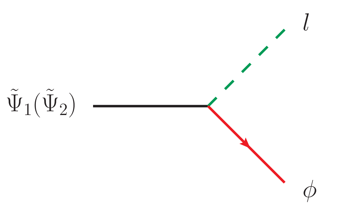
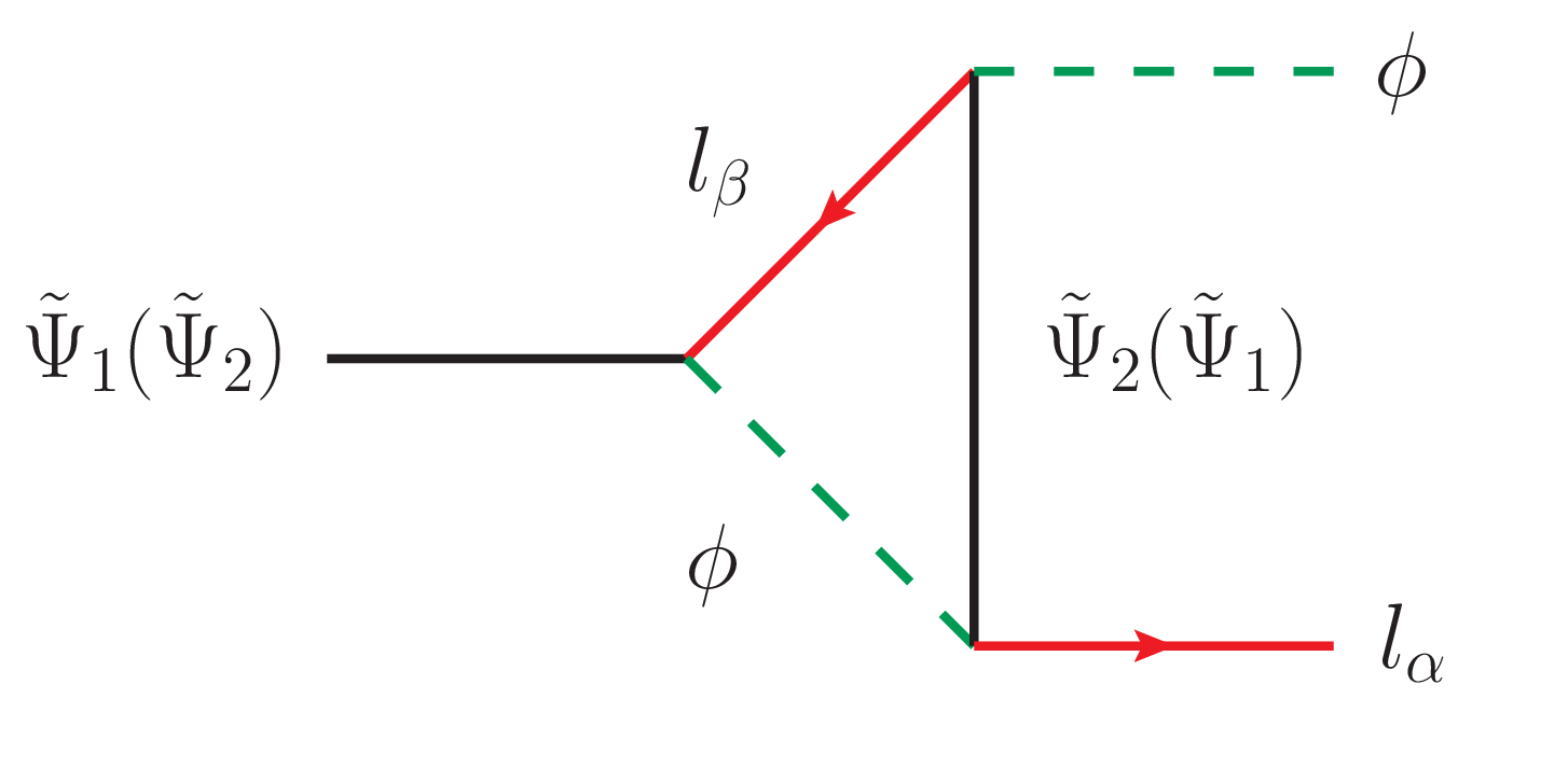
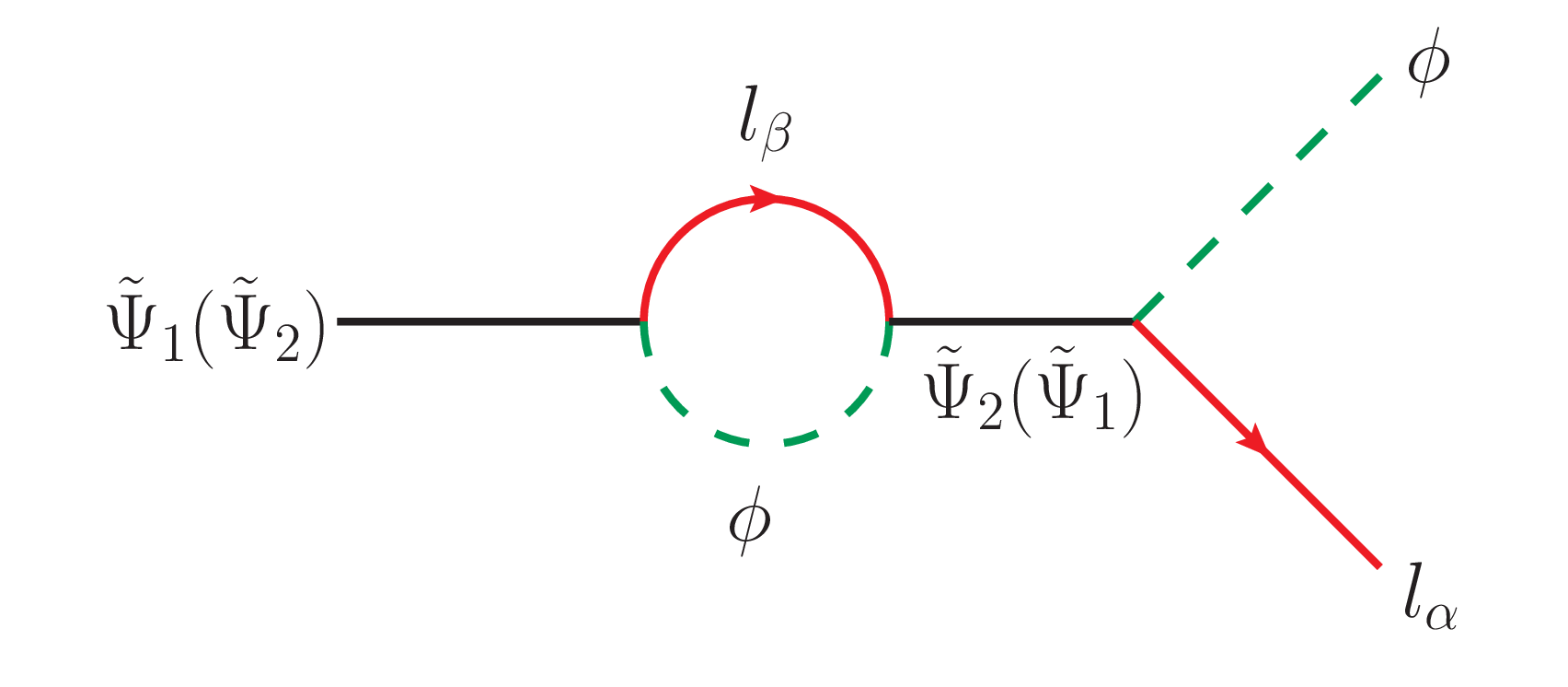
Figure 1: Diagrams contributing to the $CP$-asymmetry $\epsilon_{1}$ and $\epsilon_{2}$: (a) tree-level decay of $\tilde{\Psi_{1}}(\tilde{\Psi_{2}})$, (b) vertex correction, (c) self-energy diagram.

Assuming $M_{R}=0$, $M_{\nu}$ becomes block diagonalisable. While computing CP-asymmetry, the preferred choice of basis is that where the lower block of the $M_{\nu}$ (4 × 4 complex symmetric sub-matrix $\mathcal{M}$ ) is diagonal. In this preferred basis, the Lagrangian in Eq.(3) can be rewritten as,

$$-\mathcal{L}_{h}=h_{i\alpha}\overline{\tilde{\Psi_{i}}}\phi^{\dagger}\ell_{L_{\alpha}}+\frac{1}{2}M_{\rm diag}\tilde{\Psi_{i}}^{T}C^{-1}\tilde{\Psi_{i}}+{\rm h.c.}$$ (14)

The relations connecting Yukawa couplings in the diagonal mass basis ($h_{i\alpha}$) and the Yukawa couplings in the flavor basis ($y_{i\alpha}$) can be found in Chakraborty:2021azg . The total CP-asymmetry $\epsilon_{j}$ in the decay of $\tilde{\Psi_{j}}$ into $\ell_{\alpha}\phi~{}(\overline{\ell_{\alpha}}\phi^{\dagger})$ can be calculated by summing over the SM flavor $\beta$ as follows :

$$\epsilon_{j}=\frac{\sum_{\beta}\left[\Gamma(\tilde{\Psi_{j}}\rightarrow\ell_{\beta}\phi)-\Gamma(\tilde{\Psi_{j}}\rightarrow\overline{\ell}_{\beta}\phi^{\dagger})\right]}{\sum_{\beta}\left[\Gamma(\tilde{\Psi_{j}}\rightarrow\ell_{\beta}\phi)+\Gamma(\tilde{\Psi_{j}}\rightarrow\overline{\ell}_{\beta}\phi^{\dagger})\right]}=\frac{1}{8\pi}\sum_{i\neq j}\frac{{\rm Im}[(hh^{\dagger})_{ji}^{2}]}{(hh^{\dagger})_{jj}}f_{ji}$$ (15)

Since we are operating in the regime of resonant leptogenesis, the dominant contribution to $f_{ij}$ comes from self energy correction, i.e. $f_{ij}\sim f_{ij}^{\rm self}$, where $f_{ij}^{\rm self}=\frac{(M_{i}^{2}-M_{j}^{2})M_{i}M_{j}}{(M_{i}^{2}-M_{j}^{2})^{2}+R_{ij}^{2}}$ .

Here we have assumed that $\tilde{\Psi_{1}},\tilde{\Psi_{2}}$ are almost mass degenerate and lighter than other two states $\tilde{\Psi_{3}},\tilde{\Psi_{4}}$. Thus the computed CP-asymmetry $\epsilon_{1}$ and $\epsilon_{2}$ By solving three coupled Boltzmann equations simultaneously, one can obtain co-moving densities $Y_{\tilde{\Psi_{1}}},Y_{\tilde{\Psi_{2}}}$ and $Y_{B-L}$ of $\tilde{\Psi_{1}},\tilde{\Psi_{2}}$ and $B-L$ asymmetry respectively. The co-moving density is denoted as the ratio of actual number density and the entropy density $\overline{s}$ of the universe . The detailed presentation and discussion of the Boltzmann equations are relegated to Appendix A.

IV Collider studies

Before proceeding to perform the collider analysis, let us discuss the nature of the model parameter space in light of various constraints described in Section III. In Section II, we already have mentioned that with the inverse see-saw hierarchy, one can ascertain tiny active neutrino masses by setting $M_{R}=0$. We have also verified that this assumption hardly alters the results with respect to $M_{R}\neq 0$ scenario. Thus we set $M_{R}=0$ throughout this analysis, which in turn introduces a resemblance with the original inverse see-saw model. In addition, all the entries of $M_{\nu}$ (except $M_{R}$) are considered as complex to make the analysis a general one. While fitting the neutrino oscillation data, we adopt normal hierarchy among the light active neutrinos and also set the mass of the lightest active neutrino to be zero ($m_{1}=0$), which arises as an artifact of the present framework. For the collider analysis, we shall restrict ourselves to a particular mass region, where the mass of the lightest heavy neutrino ($M_{\tilde{\Psi_{1}}}$) is less than or equal to 10 TeV, i.e. $M_{\tilde{\Psi_{1}}}\leq~{}10$ TeV. Now, the ranges for input parameters for the aforementioned range of $M_{\tilde{\Psi_{1}}}$ are : $M_{D_{i,j}}^{R,I}\in[10^{7}~{}{\rm eV}:10^{8}~{}{\rm eV}]$ , $M_{S_{i,j}}^{R,I}\in[10^{10}~{}{\rm eV}:10^{14}~{}{\rm eV}]$. From Eq.(11) one can solve $\mu$ and express it in terms of the input parameters $M_{D},M_{S}$ ( with $M_{R}=0$ ) and neutrino oscillation parameters. In addition, it has been verified that in presence of the TeV scale heavy neutrinos, the most stringent bound coming from the LFV decay $\mu\to e\gamma$ TheMEG:2016wtm , can be easily evaded throughout the parameter space. Next by solving the Boltzmann equations (given in Appendix A), one can compute the baryon asymmetry of the universe at each and every point of the parameter space. In Fig.2(a) (Fig.2(b)), we have plotted Br($\mu\to e\gamma$) vs. $M_{\tilde{\Psi_{1}}}~{}(M_{\tilde{\Psi_{3}}})$. The blue, red and green points are compatible with neutrino oscillation data only, neutrino oscillation data + LFV decay and neutrino oscillation data + LFV decay + current baryon asymmetry of the universe respectively. Here we have considered a 1$\sigma$ deviation around the central value of observed baryon asymmetry (Eq.(1)).

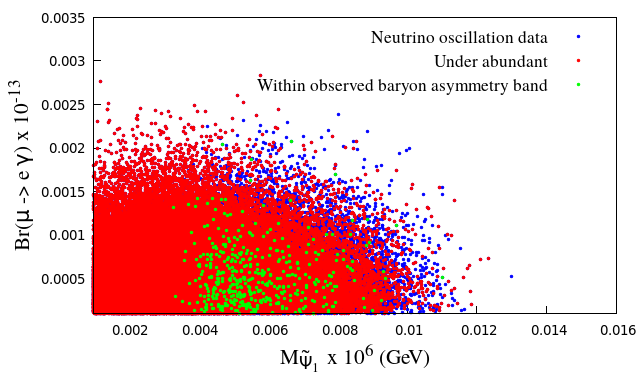
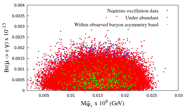
Figure 2: Branching ratios of radiative decay of muon ($\mu\rightarrow e\gamma$) with the mass of the heavy neutrinos ((a)$M_{\tilde{\Psi_{1}}}$, (b) $M_{\tilde{\Psi_{3}}}$). Color codes represent points satisfy the neutrino oscillation data (blue), observed baryon asymmetry (green) and under abundance (red).

In one of our previous studies Chakraborty:2021azg , we have shown that there exists a stringent lower bound of $\sim$ 3.2 TeV on $M_{\tilde{\Psi_{1}}}$ to satisfy the current baryon asymmetry data. For performing collider analysis, we shall choose eight benchmark points (BP1, BP2, BP3, BP4, BP5, BP6, BP7, BP8) from the model parameter space, which lie well within the correct baryon asymmetry band. Thus the chosen benchmark points are compatible with the experimental data coming from neutrino oscillation, LFV decays and current baryon asymmetry of the universe. These benchmark points are characterised by low, medium and high lightest heavy neutrino masses ($M_{\tilde{\Psi_{1}}}$), spanning a wide range, from 3.2 TeV to 10.12 TeV. The eight benchmarks are tabulated in Table 2 along with $M_{\tilde{\Psi}_{1(2)}}$, $M_{\tilde{\Psi}_{3(4)}}$ and corresponding baryon asymmetry yield. To probe the benchmark points, we perform the collider analysis at two COMs ($\sqrt{s}$), i.e. $\sqrt{s}=6$ TeV (for BP1, BP2, BP3) , 14 TeV (for BP4, BP5, BP6, BP7, BP8) at muon collider.

In the next subsection we shall perform the collider analysis of the $2l+E_{T}/\;\>$ final state, which turns out to be promising at aforementioned COMs. Owing to small signal cross section, even with high luminosity, this signal turns out to be non-promising at LHC. We shall provide a comparative study with LHC later. Besides, this signal involving TeV scale heavy neutrinos in the final state cannot be probed at ILC since the maximum achievable COM at ILC is 1 TeV. The leading order (LO) signal and background cross sections are generated via MG5aMC@NLO Alwall:2014hca . Further decays of the unstable particles are emulated through Pythia8 Sjostrand:2014zea . The detector effects are included in the analysis by passing both the signal and the backgrounds through Delphes-3.5.0 deFavereau:2013fsa . We use the default muon collider simulation card muoncollidercardTalk for this purpose. Since traditional cut-based analysis is enough to yield high significances for all benchmarks, we shall only present the results generated from it. The signal significance has been computed using $\mathcal{S}=\sqrt{2\Big{[}(S+B)\log\Big{(}\frac{S+B}{B}\Big{)}-S\Big{]}}$ Cowan:2010js , where $S(B)$ denote the number of signal (background) events surviving the cuts applied on relevant kinematic variables.

Benchmark	$M_{\tilde{\Psi}_{1}}{\displaystyle\simeq}M_{\tilde{\Psi}_{2}}$	$M_{\tilde{\Psi}_{3}}{\displaystyle\simeq}M_{\tilde{\Psi}_{4}}$	Baryon asymmetry ($Y_{B}$)
Points	$(\rm TeV)$	$(\rm TeV)$
BP1	3.28	12.31	8.677$\rm\times 10^{-11}$
BP2	4.01	20.18	8.884 $\rm\times 10^{-11}$
BP3	5.11	16.69	8.639 $\rm\times 10^{-11}$
BP4	6.33	16.23	8.708 $\rm\times 10^{-11}$
BP5	7.38	16.64	8.522 $\rm\times 10^{-11}$
BP6	8.24	19.23	8.767 $\rm\times 10^{-11}$
BP7	9.31	17.49	8.688 $\rm\times 10^{-11}$
BP8	10.12	17.18	8.713 $\rm\times 10^{-11}$

Table 2: Masses of Heavy Neutrinos along with the baryon asymmetry for eight benchmarks.

IV.1 $2l+E_{T}/\;\>$ final state

In muon collider, heavy neutrinos can be produced along with active neutrinos via $t$-channel $W^{\pm}$ mediation and $s$-channel $Z$ mediation. In this analysis, we aim to probe the following signal shown in Fig.6(a),(b) leading to $2l+\not\!E_{T}$ final state:

$$\mu^{+}\mu^{-}\to\nu_{l}~{}\tilde{\Psi}_{1(2)};$$

$$\tilde{\Psi}_{1(2)}\to W^{\pm}~{}l^{\mp};~{}W^{\pm}\to l^{\pm}\nu_{l}(\overline{\nu}_{l});$$

$$\to~{}l^{+}l^{-}+\not\!E_{T}$$ (17)

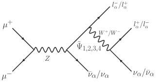
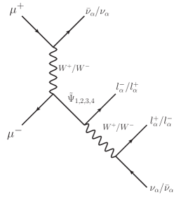
Figure 3: The Feynman diagrams representing the signal process $\mu^{+}\mu^{-}\rightarrow 2l+E_{T}/\;\>$. In these diagrams, $l^{\pm}_{\alpha}$ denote $e,\mu$.

Here, the heavy neutrino can decay to $W^{\pm}$ via charged current interaction which is further accompanied by the leptonic decay of $W^{\pm}$. Here we consider the leptonic decay mode of $W^{\pm}$ as it can provide a clean signature. The dominant background for this signal originates from the $\mu^{+}\mu^{-}\to l^{+}l^{-}+\not\!E_{T}$ final state, which receives contributions from the following sub-processes :

• $\mu^{+}\mu^{-}\to W^{+}W^{-}$; $W^{+}\to l^{+}~{}\nu_{\ell},~{}W^{-}\to l^{-}~{}\overline{\nu}_{\ell}$,

• $\mu^{+}\mu^{-}\to ZZ$; $Z\to l^{+}l^{-},~{}Z\to\nu_{l}~{}\overline{\nu}_{l}$,

• $\mu^{+}\mu^{-}\to W^{+}W^{-}Z$; $W^{+}\to l^{+}~{}\nu_{l},~{}W^{-}\to l^{-}~{}\overline{\nu}_{l},~{}Z\to\nu_{l}~{}\overline{\nu}_{l}$,

• $\mu^{+}\mu^{-}\to ZZZ$; $Z\to l^{+}l^{-},~{}Z\to\nu_{l}~{}\overline{\nu}_{l},~{}Z\to\nu_{l}~{}\overline{\nu}_{l}$.

Signal / Backgrounds	Process	Cross section $\sigma$ (LO) (fb)
	6 TeV
Signal
BP1		244
BP2	$\mu^{+}\mu^{-}\rightarrow 2l+E_{T}/\;\>$	36
BP3		3
Background	$\mu^{+}\mu^{-}\rightarrow 2l+E_{T}/\;\>$	233
	14 TeV
Signal
BP4		44.95
BP5		8.29
BP6	$\mu^{+}\mu^{-}\rightarrow 2l+E_{T}/\;\>$	2.33
BP7		0.78
BP8		0.18
Background	$\mu^{+}\mu^{-}\rightarrow 2l+E_{T}/\;\>$	187.34

Table 3: The LO cross sections for signal and backgrounds for the process $\mu^{+}\mu^{-}\rightarrow 2l+E_{T}/\;\>$ at 6 TeV and 14 TeV.

The LO cross sections of the signals (for all benchmarks) and SM backgrounds are tabulated in Table 3. To reduce the background with respect to signal, we choose a set of cuts over kinematic variables. We classify the cuts on the kinematic variables for benchmarks BP1- BP3 at 6 TeV COM energy as $B_{i}~{}(i:1-7)$ and for the rest of the benchmarks (BP4-BP8) at $\sqrt{s}=14$ TeV, the cuts are defined as $C_{j}~{}(j:1-7)$. For brevity, and also to avoid repetition, we discuss the cuts for two different COM energies together. All the names of the cuts or numbers within the bracket below will correspond to 14 TeV COM energy. Following are the depiction of cuts chosen to enhance significance:

• ${B_{1}~{}(C_{1}):}$ We demand two opposite sign, same or different flavored charged leptons $l$ in the final state. Here $l$ denotes only electron and/or muon.

• ${B_{2}~{}(C_{2}):}$ The normalized distributions of the transverse momentum of the leading lepton ($p_{T_{l_{1}}}$) for signal and background are shown in Fig.4(a) (Fig.5(a)). Here the leading lepton gets the boost in $p_{T}$ from the COM energy directly for the signal. Thus $p_{T_{l_{1}}}$ for the signal peaks at a larger value with respect to the SM background. Thus putting a large lower cut on the transverse momentum, i.e. $p_{T_{l_{1}}}>400~{}(200)$ GeV can be a suitable choice to enhance the signal significance.

• $B_{3}$: We show the normalized distributions of the transverse momentum of the next to leading lepton ($p_{T_{l_{2}}}$) for signal and backgrounds in Fig.4(b). As can be seen from the distributions, the SM background peaks around $p_{T}\sim 0$, because the major fraction of the transverse momentum is taken away by the leading lepton. The signal distribution starts dominating the background distribution after 200 GeV. Therefore, we put a lower cut of $p_{T_{l_{2}}}>200$ GeV to maximise the significance.

• $C_{3}:$ We depict the normalized distributions of scalar sum of the transverse momenta of two leptons in the final state in Fig.5(b). The nature of the distributions of the signal and background can be explained following the descriptions of the distributions of $p_{T_{l_{1}}}$ and $p_{T_{l_{2}}}$ in previously defined cuts B2(C2) and B3. A suitable lower cut : $p_{T}^{l_{1},l_{2}}>2$ TeV helps magnifying the significance drastically.

• $B_{4}~{}(C_{4}):$ In Fig.4(c) (Fig.5(c)), we plot the normalised distributions of the magnitude of the vector sum of the transverse momenta of two leptons in the final state for signal and background. It is defined as:

  $$p^{vect}_{T_{l_{1},l_{2}}}\equiv\sqrt{(p_{{Tx}_{l_{1}}}+p_{{Tx}_{l_{2}}})^{2}+(p_{{Ty}_{l_{1}}}+p_{{Ty}_{l_{2}}})^{2}+(p_{{Tz}_{l_{1}}}+p_{{Tz}_{l_{2}}})^{2}}$$

  Here, $p_{{Tx}_{l_{i}}},p_{{Ty}_{l_{i}}}$ and $p_{{Tz}_{l_{i}}}$ are the $x,y,z$-components of the transverse momentum vector for $i=1,2$ respectively. We choose $p^{vect}_{T_{l_{1},l_{2}}}>600(2000)$ GeV to suppress SM background.

• $B_{5}:$ We define a kinematic variable $M_{eff}$, i.e. effective mass as the scalar sum of the transverse momenta of the final state leptons and missing transverse energy. The normalized distributions of $M_{eff}$ both for signal and background are shown in Fig.4(d). The distributions mimic the distributions for individual transverse momentum of the final state leptons as expected. Since the signal distributions for almost all benchmarks start overshadowing the SM background distribution for $M_{eff}>2000$ GeV, to achieve large significance, we choose $M_{eff}>2000$ GeV.

• $B_{6}~{}(C_{5})$: We portray the normalized distribution of $\Delta R_{l_{1}l_{2}}$ for signals and backgrounds in Fig.4(e)(Fig.5(d)). It is evident from the distributions of the signal and background, a proper cut of $\Delta R_{l_{1}l_{2}}>3.0(3.0)$ has been chosen to distinguish the signal from the background.

• $B_{7}~{}(C_{6})$: We compute the magnitude of azimuthal angular separation of two final state leptons as:

  $$\Delta\phi_{l_{1}l_{2}}=|\phi_{l_{1}}-\phi_{l_{2}}|\text{ for $\Delta\phi_{l_{1}l_{2}}<\pi$}$$

  $$\Delta\phi_{l_{1}l_{2}}=2\pi-|\phi_{l_{1}}-\phi_{l_{2}}|,\text{ otherwise}$$

  The normalized distributions of $\Delta\phi_{l_{1}l_{2}}$ are presented in Fig.4(f) (Fig.5(e)). We choose $\Delta\phi_{l_{1}l_{2}}>3.0(3.1)$, for the survival of the signal over background.

• $C_{7}:$ We define the azimuthal angular separation between direction of the leading lepton $l_{1}$ and missing energy vector $\cancel{E}_{T}$ as $\Delta\phi_{l_{1},~{}\cancel{E}_{T}}$ and show the normalized distributions of the same in Fig.5(f). To differentiate the signal from the background, most optimal cut on the aforementioned variable is $\Delta\phi_{l_{1},~{}\cancel{E}_{T}}>3.1$.

We summarize the results obtained after each cut, i.e. $(B_{1}-B_{7})$ for $\sqrt{s}=6$ TeV and $(C_{1}-C_{7})$ for $\sqrt{s}=14$ TeV mentioned above in two tables. The cut-flow of the first three benchmarks along with the SM background for COM 6 TeV are presented in Table 4. The number of signal and background events after applying each cut are quoted at integrated luminosity 100 fb^-1. It is evident from the table that the cuts are very effective to wipe out the background compare to the signal. At $\sqrt{s}=6$ TeV and $\mathcal{L}=100$ fb^-1, we are left with only 192 background events. Whereas the signal events remains almost steady after applying the same cuts. In the last column of the table, we compute the required integrated luminosity to achieve the 5$\sigma$ significance. For BP1, 0.2 ${\rm fb}^{-1}$ luminosity is enough to achieve $5\sigma$ significance while a benchmark with higher heavy neutrino mass 5.11 TeV (BP3) would require 9.1 ${\rm fb}^{-1}$. This happens owing to the decrease in signal cross section with increasing $M_{\tilde{\Psi}_{1}}$.

Next in Table 5, we present the cut flow for benchmarks BP4-BP8 for COM energy 14 TeV with integrated luminosity 1600 ${\rm fb}^{-1}$. SM background events are reduced to 237 after employing all the chosen cuts. Whereas the number of the signal events surviving after imposing all cuts are 25809 (for BP4), 4698 (for BP5), 1323 (for BP6), 430 (for BP7), and 98 (for BP8). In addition, we derive the integrated luminosity needed to attain $5\sigma$ significance. For BP4-BP8, 2 ${\rm fb}^{-1}$, 9 ${\rm fb}^{-1}$, 36 ${\rm fb}^{-1}$, 144 ${\rm fb}^{-1}$ and 1381 ${\rm fb}^{-1}$ integrated luminosities are required to achieve 5$\sigma$ discovery. Thus one can conclude that the benchmark with larger cross section and hence with smaller value of $M_{\tilde{\Psi}_{1}}$, is more promising to probe at the muon collider than others.

	Number of Events after cuts ($\mathcal{L}=100$ fb-1)
SM-background	$B_{1}$	$B_{2}$	$B_{3}$	$B_{4}$	$B_{5}$	$B_{6}$	$B_{7}$
$2l+E_{T}/\;\>$	19040	4839	2230	1622	624	396	192
Signal								$\mathcal{L}_{5\sigma}$ (fb-1)
BP1	19176	18239	17427	16672	15348	15113	14656	0.2
BP2	2825	2683	2566	2440	2227	2195	2128	1.2
BP3	393	373	355	336	306	302	292	9.1

Table 4: The cut-flow for signal and backgrounds along with the significances for BP1, BP2 and BP3 at 6 TeV Muon collider and the required integrated luminosity for 5$\sigma$ significance for the $\mu^{+}\mu^{-}\rightarrow 2l+E_{T}/\;\>$ channel.

	Number of Events after cuts ($\mathcal{L}=1600$ fb-1)
SM-background	$C_{1}$	$C_{2}$	$C_{3}$	$C_{4}$	$C_{5}$	$C_{6}$	$C_{7}$
$2l+E_{T}/\;\>$	239257	73455	13677	9070	5676	1094	237
Signal								$\mathcal{L}_{5\sigma}$ (fb-1)
BP4	54794	54637	53629	48035	47547	40009	25809	2
BP5	10079	10046	9878	8804	8709	7332	4698	9
BP6	2834	2825	2770	2460	2432	2052	1323	36
BP7	947	944	925	810	801	672	430	144
BP8	217	216	211	186	184	154	98	1381

Table 5: The cut-flow for signal and backgrounds along with the significances for BP4, BP5, BP6, BP7 and BP8 at 14 TeV Muon collider and the required integrated luminosity for 5$\sigma$ significance for the $\mu^{+}\mu^{-}\rightarrow 2l+E_{T}/\;\>$ channel.

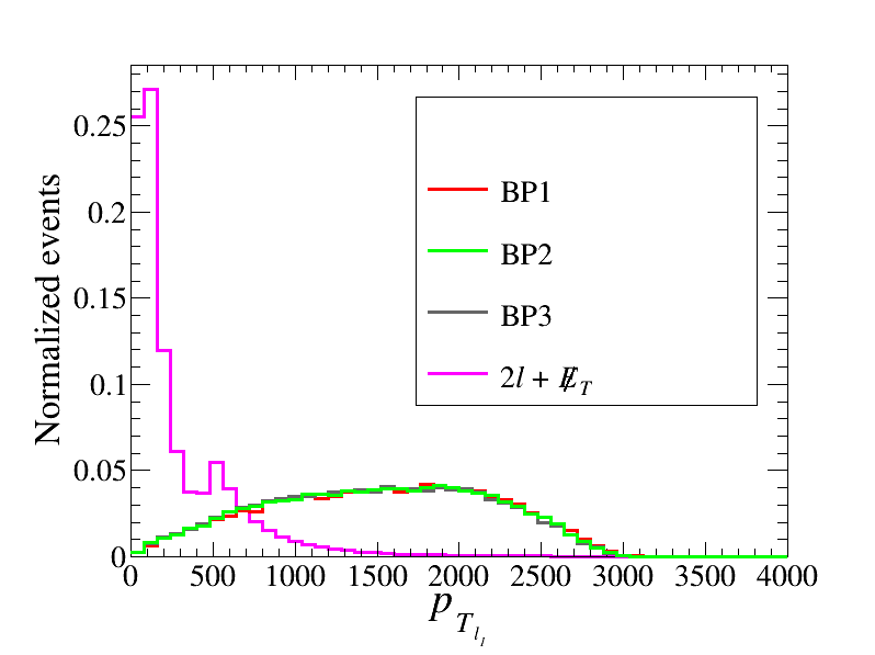
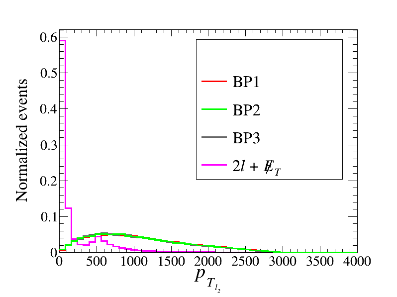
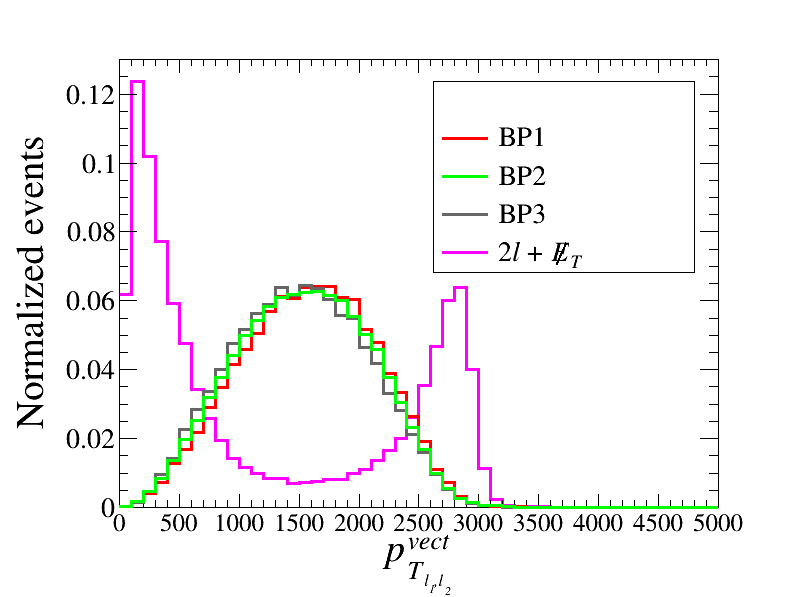
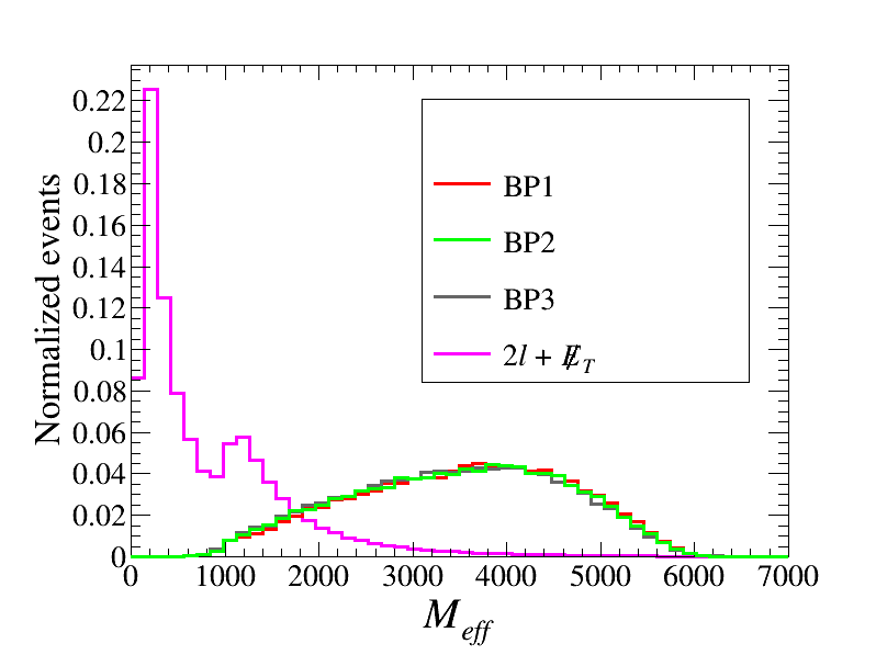
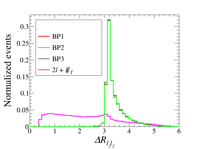
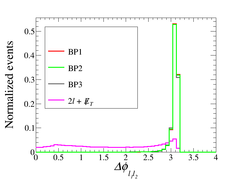
Figure 4: Distributions of normalized events for signal and SM background considering first three benchmarks (BP1-BP3) at 6 TeV COM, with the kinematic variables: (a) $p_{T_{l_{1}}}$, (b) $p_{T_{l_{2}}}$, (c) $p^{vect}_{T_{l_{1},l_{2}}}$, (d) $M_{\text{eff}}$, (e) $\Delta R_{l_{1}l_{2}}$, (f) $\Delta\phi_{l_{1}l_{2}}$.

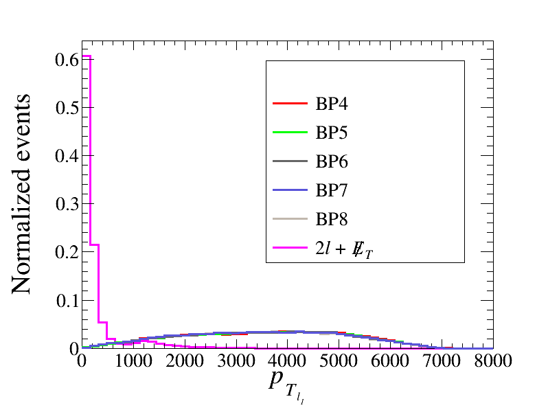
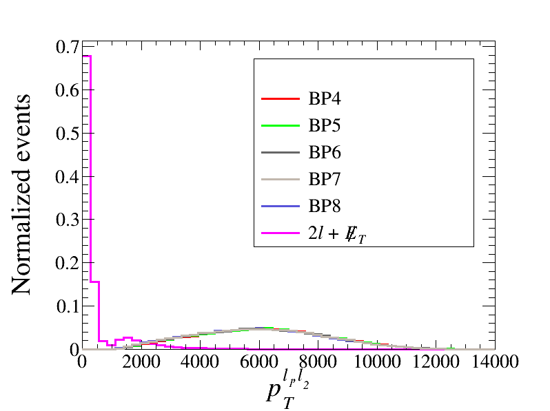
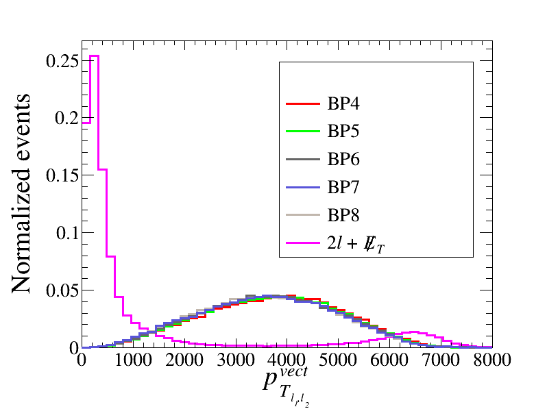
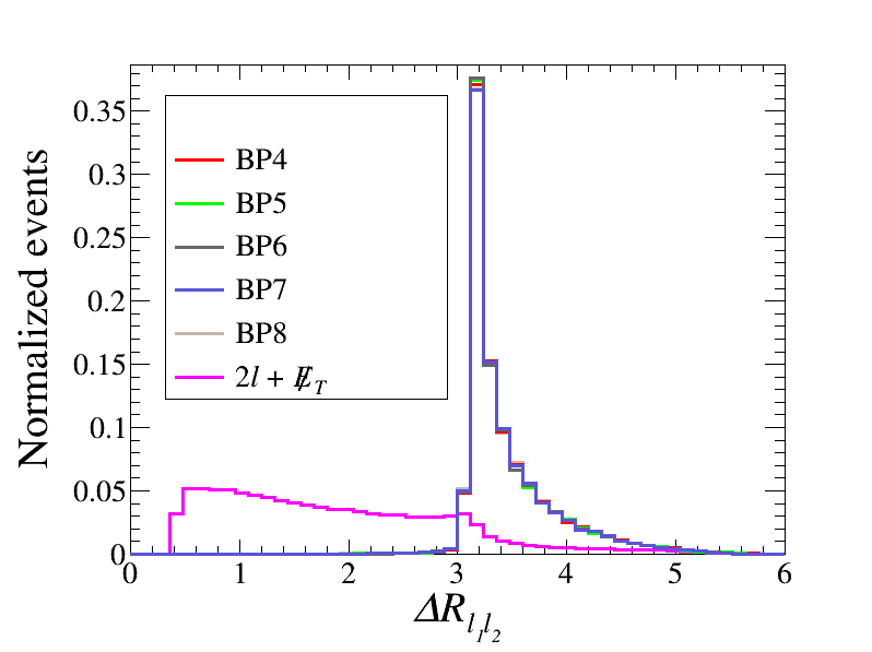
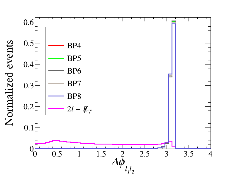
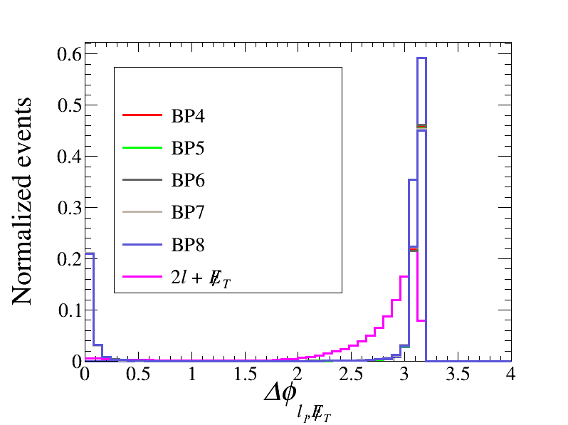
Figure 5: Distributions of normalized events for signal and SM background considering benchmarks (BP4-BP8) at 14 TeV COM, with the kinematic variables: (a) $p_{T_{l_{1}}}$, (b) $p_{T}^{l_{1},l_{2}}$, (c) $p_{T_{l_{1}l_{2}}}^{vect}$, (d) $\Delta R_{l_{1}l_{2}}$, (e) $\Delta\phi_{l_{1}l_{2}}$, (f) $\Delta\phi_{l_{1}\cancel{E}_{T}}$

.

V Summary and conclusion

In this present paper, we have focused on a framework popularly known as ISS(2,2), i.e. (2,2) inverse see-saw realisation, where the SM is accompanied with two singlet right handed neutrinos and two singlet neutral fermions. From the name of the model itself, it is evident that the neutrino mass generation in this scenario occurs via inverse see-saw mechanism. To make the analysis a robust one, we have considered the most general structure of the $7\times 7$ neutrino mass matrix $M_{\nu}$ with complex entries. Further by regulating the input model parameters and assuming normal mass hierarchy between the active neutrinos, we can segregate the portion of the parameter space, which becomes compatible with the neutrino oscillation data. Upon diagonalising the mass matrix $M_{\nu}$, we are left with three active neutrino and four heavy neutrino mass eigenstates ($\tilde{\Psi_{1}},\tilde{\Psi_{2}},\tilde{\Psi_{3}},\tilde{\Psi_{4}}$). The interesting feature of these heavy neutrino mass eigenstates is the pairwise mass degeneracy of the same, i.e. $M_{\tilde{\Psi_{1}}}\simeq M_{\tilde{\Psi_{2}}}$ and $M_{\tilde{\Psi_{3}}}\simeq M_{\tilde{\Psi_{4}}}$. In addition, we have checked that the former parameter space also obeys the bounds coming from the LFV decays. Next at each and every point in the parameter space satisfying neutrino oscillation data and the bounds coming from the LFV decays, the baryon asymmetry is computed. Thus we can obtain a subset of the larger parameter space, which is compatible with (i) neutrino oscillation data, (ii) constraints coming from LFV decay and (iii) observed baryon asymmetry data. One can conclude that the baryon asymmetry constraint itself has put a lower bound on the lightest heavy neutrino state i.e. $M_{\tilde{\Psi_{1}}}>3.2$ TeV.

Next we aim to analyse some promising collider signatures at multi-TeV muon collider. First we choose some benchmark points from the previously derived parameter space, depending on $M_{\tilde{\Psi_{1}}}$. For collider study, we intend to analyse those benchmarks which satisfy the observed baryon asymmetry of the universe. Accordingly, we have picked up different benchmarks where $M_{\tilde{\Psi_{1}}}$ ranges between 3.2 TeV to 10.3 TeV (BP1-BP8).The range of heavy neutrino masses which we are talking about, cannot be produced at ILC. The signal contains pair production of active neutrino and a heavy neutrino, followed by the decay of the heavy neutrino into $W^{\pm}$ and a charged lepton (e, $\mu$). Further if we consider the leptonic decay of the generated $W^{\pm}$, it will lead to a di-lepton plus missing energy state. For analysis, we choose $\sqrt{s}=6$ TeV for BP1, BP2 and BP3 and $\sqrt{s}=14$ TeV for the rest of the benchmarks (BP4-BP8). We have not considered conventional LHC or ILC for purpose. The cross-section of the same process at LHC is much smaller than what we obtained in muon-collider. In addition, the large LHC backgrounds would be sufficient to kill the signal. The disadvantage of ILC lies in the maximal achievable COM energy (1 TeV). The dominant background for this signal is $2l+E_{T}/\;\>$, arising from the subprocesses like $W^{+}W^{-},~{}ZZ,~{}W^{+}W^{-}Z,~{}ZZZ$. Here we impose cuts on a few relevant kinematic variables to achieve maximally enhanced signal significances, suppressing the backgrounds with respect to the signals. Among all benchmarks, BP1 (BP4) turns out to be most promising with respect to the analysed signal at $\sqrt{s}=6$ TeV (14 TeV). To achieve 5$\sigma$ significance one needs 0.2 fb^-1, 1.2 fb^-1 and 9.1 fb^-1 integrated luminosity for BP1, BP2, BP3v respectively at COM energy 6 TeV. Besides the integrated luminosities required for 5$\sigma$ significance are 2 fb^-1, 9 fb^-1, 36 fb^-1, 144 fb^-1, 1381 fb^-1 respectively for BP4, BP5, BP6, BP7, BP8 at $\sqrt{s}=14$ TeV. Though this particular channel provides encouraging results at muon collider, one can also consider the hadronic decay of $W^{\pm}$ in the signal instead of leptonic decay, leading to $1l+2j+E_{T}/\;\>$ signature. Analysing this channel could be challenging due to the presence of large jetty SM backgrounds. We shall present a comprehensive analysis of this channel separately for comparison.

VI ACKNOWLEDGEMENTS

The authors thank Aleksander Filip Zarnecki, Yongcheng Wu, Nabarun Chakrabarty and Gourab Saha for technical help and fruitful discussions. IC acknowledges support from DST, India, under grant number IFA18-PH214 (INSPIRE Faculty Award). HR is supported by the Science and Engineering Research Board, Government of India, under the agreement SERB/PHY/2016348 (Early Career Research Award). TS acknowledges the support from the Dr. D. S. Kothari Postdoctoral scheme No. PH/20-21/0163.

Appendix A Evolution of asymmetry

Evolution of asymmetry can be calculated by solving the following Boltzmann equations: $\tilde{\Psi_{1}},\tilde{\Psi_{2}}$ and the $(B-L)$ asymmetry can be written as Plumacher:1996kc ,

$$\frac{\text{d}Y_{\tilde{\Psi_{1}}}}{\text{d}z} = -\frac{z}{s\hskip 2.84526ptH(M_{\tilde{\Psi_{1}}})}\Big{[}\Big{(}\frac{Y_{\tilde{\Psi_{1}}}}{Y^{eq}_{\tilde{\Psi_{1}}}}-1\Big{)}(\gamma_{D}^{(1)}+2\gamma^{(1)}_{\phi,s}+4\gamma^{(1)}_{\phi,t})\Big{]}\,,$$ (18)

$$\frac{\text{d}Y_{\tilde{\Psi_{2}}}}{\text{d}z} = -\frac{z}{s\hskip 2.84526ptH(M_{\tilde{\Psi_{1}}})}\Big{[}\Big{(}\frac{Y_{\tilde{\Psi_{2}}}}{Y^{eq}_{\tilde{\Psi_{2}}}}-1\Big{)}(\gamma_{D}^{(2)}+2\gamma^{(2)}_{\phi,s}+4\gamma^{(2)}_{\phi,t})\Big{]}\,,$$ (19)

$$\frac{\text{d}Y_{B-L}}{\text{d}z} = -\frac{z}{s\hskip 2.84526ptH(M_{\tilde{\Psi_{1}}})}\Big{[}\sum_{j=1}^{2}\left\{\frac{1}{2}\frac{Y_{B-L}}{Y^{eq}_{l}}+\epsilon_{j}~{}\Big{(}\frac{Y_{\tilde{\Psi_{j}}}}{Y^{eq}_{\tilde{\Psi_{j}}}}-1\Big{)}\right\}\gamma_{D}^{(j)}$$ (20)

$$+\frac{Y_{B-L}}{Y^{eq}_{l}}\left\{2\gamma_{\tilde{\Psi},s}+2\gamma_{\tilde{\Psi},t}\right\}+\frac{Y_{B-L}}{Y^{eq}_{l}}\sum_{j=1}^{2}\left\{2\gamma^{(j)}_{\phi,t}+\frac{Y_{\tilde{\Psi_{j}}}}{Y^{eq}_{\tilde{\Psi_{j}}}}\gamma^{(j)}_{\phi,s}\right\}\Big{]}\,,$$

where $z=\frac{M_{\tilde{\Psi_{1}}}}{T}$ and $H(M_{\tilde{\Psi_{1}}})$ is the Hubble parameter at $T=M_{\tilde{\Psi_{1}}}$ and $H(T=M_{\tilde{\Psi_{1}}})=1.66~{}g_{eff}^{1/2}\frac{T^{2}}{M_{\rm{Pl}}}|_{T=M_{\tilde{\Psi_{1}}}}$, $M_{\rm{Pl}}\sim 10^{19}$ GeV being Planck scale. $Y_{\tilde{\Psi_{j}}}^{eq},Y_{l}^{eq}$ are the comoving densities at equilibrium. We solve these three equations with initial conditions :

$$Y_{\tilde{\Psi_{i}}}(0)=Y_{\tilde{\Psi_{i}}}^{eq},~{}{\rm and}~{}Y_{B-L}(0)=0\,.$$ (21)

at $T>>M_{\tilde{\Psi_{1}}}$.

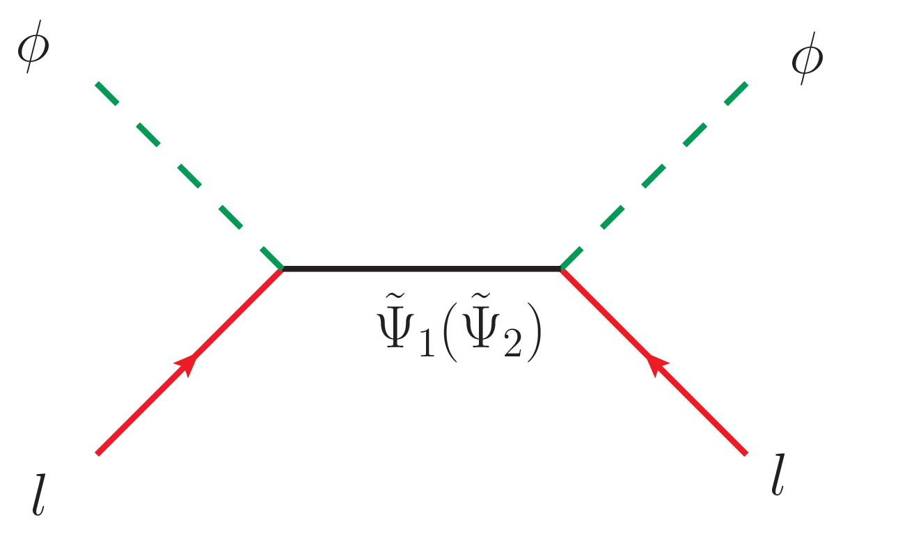
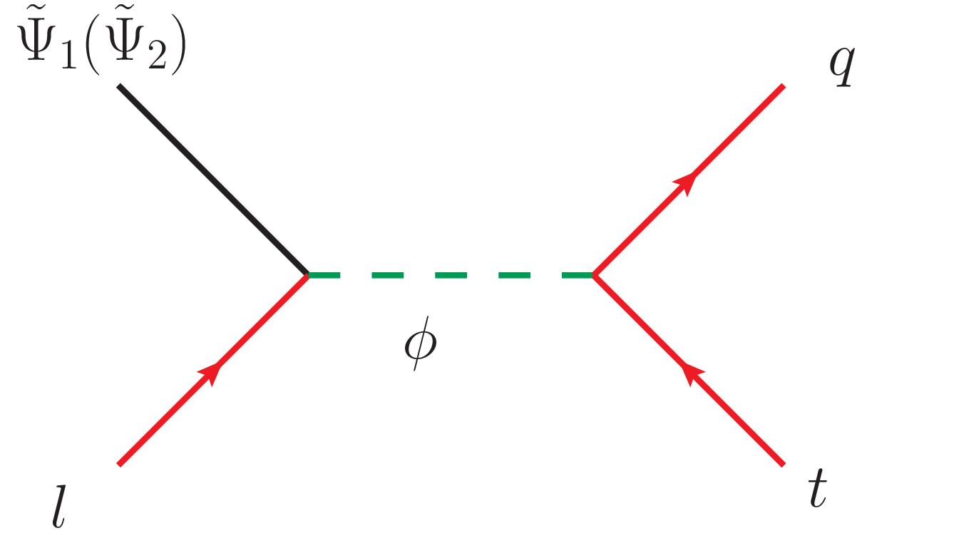
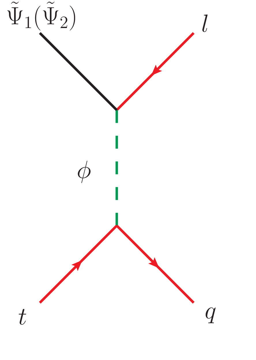
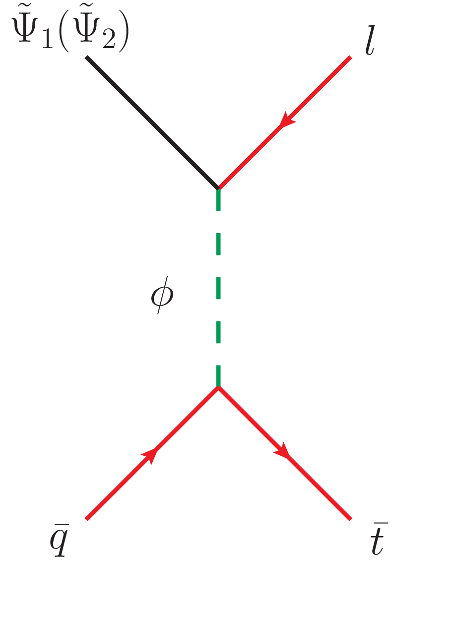
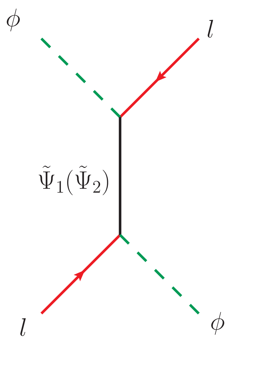
Figure 6: Feynman diagram representing (a) decay of lightest heavy RH-neutrino $\tilde{\Psi_{1}}~{}(\tilde{\Psi_{2}})$ (contributes to $\gamma_{D}^{(1)},\gamma_{D}^{(2)}$), (b) $\Delta L=2$, $s$-channel scattering via $\tilde{\Psi_{1}}~{}(\tilde{\Psi_{2}})$ (contributes to $\gamma_{\tilde{\Psi},s}$), (c) $\Delta L=1$, $s$-channel scattering via Higgs (contributes to $\gamma^{1}_{\phi,s},\gamma^{2}_{\phi,s}$), (d) and (e) $\Delta L=1$, $t$-channel scattering via Higgs (contributes to $\gamma^{1}_{\phi,t},\gamma^{2}_{\phi,t}$), (f) $\Delta L=2$, $t$-channel scattering via $\tilde{\Psi_{1}}~{}(\tilde{\Psi_{2}})$ (contributes to $\gamma_{\tilde{\Psi},t}$).

Contributions to $\gamma^{{}^{\prime}}$s are given by diagrams shown in Fig. 6.

The lepton asymmetry is further can be translated into baryon asymmetry. This results in the final baryon number at $T_{\rm sph}\sim 150$ GeV (the freeze-out temperature of the sphelaron process ) as Burnier:2005hp :

$$Y_{B}=\bigg{(}\frac{8N_{f}+4N_{H}}{22N_{f}+13N_{H}}\bigg{)}Y_{B-L}(z_{\rm sph}).$$ (22)

With $Y_{B-L}(z_{\rm sph})$ as the solution of Boltzmann equations at $z=z_{\rm sph}=\frac{M_{\tilde{\Psi_{1}}}}{T_{\rm sph}}$.

Here $N_{f}:$ the number of generations of fermion families and $N_{H}:$ number of Higgs doublets. For our case, $N_{f}=3$ and $N_{H}=1$. $\gamma_{D}^{(i)}$ can be written as Plumacher:1996kc :

$$\gamma_{D}^{(i)}=N_{\tilde{\Psi}_{i}}^{eq}~{}\frac{K_{1}(\frac{M_{\tilde{\Psi}_{i}}}{T})}{K_{2}(\frac{M_{\tilde{\Psi}_{i}}}{T})}~{}\Gamma_{\tilde{\Psi_{i}}}\,,{\rm with}~{}i=2$$ (23)

$N_{\tilde{\Psi}_{i}}^{eq}$ being the equilibrium number density of mass eigenstate $\tilde{\Psi}_{i}$. Here $K_{1}$ and $K_{2}$ are the first and second modified Bessel functions of second kind respectively and $\Gamma_{\tilde{\Psi}_{i}}$ is the total decay width of $\tilde{\Psi}_{i}$.

Decay width of $\tilde{\Psi}_{i}$ at tree level,

$$\Gamma_{\tilde{\Psi}_{i}} := \Gamma(\tilde{\Psi}_{i}\rightarrow\phi^{\dagger}+l)+\Gamma(\tilde{\Psi}_{i}\rightarrow\phi+\overline{l})$$ (24)

$$=\frac{\alpha}{\text{sin}^{2}\theta_{W}}\frac{M_{\tilde{\Psi}_{i}}}{4}\frac{(M^{\dagger}_{D}M_{D})_{ii}}{M^{2}_{W}}$$

with $\alpha,\theta_{W}$ being the Fine structure constant and the Weinberg angle.

For two body scattering $a+b\rightarrow i+j+...$, $\gamma_{eq}$ can be written as Plumacher:1996kc ,

$$\gamma_{eq}=\frac{T}{64\pi^{4}}\int_{(M_{a}+M_{b})^{2}}^{\infty}\hskip 2.84526ptds~{}\hat{\sigma}(s)\hskip 2.84526pt\sqrt{s}\hskip 2.84526ptK_{1}(\frac{\sqrt{s}}{T})\,.$$ (25)

here $s$ is the square of center of mass energy and $\hat{\sigma}(s)$ is reduced cross section, which can be expressed in terms of actual cross section as Plumacher:1996kc :

$$\hat{\sigma}(s)=\frac{8}{s}\left[(p_{a}.p_{b})^{2}-M_{a}^{2}M_{b}^{2}\right]\sigma(s)\,,$$ (26)

with $p_{k}$ and $M_{k}$ being three momentum and mass of particle $k$. Expressions for reduced cross-section ($\hat{\sigma}$) for all the scattering processes shown in Fig. 6 are given in Plumacher:1996kc ; Chakraborty:2021azg .

For our model the total D.O.F turns out to be :

$$g_{eff}~{}(T>174~{}{\rm GeV}) = g_{\rm boson}+g_{\rm fermion}$$ (27)

$$28+\frac{7}{8}\times 94=110.25$$

References

- (1) ATLAS collaboration, G. Aad et al., Observation of a new particle in the search for the Standard Model Higgs boson with the ATLAS detector at the LHC, Phys. Lett. B 716 (2012) 1–29, [1207.7214].
- (2) CMS collaboration, S. Chatrchyan et al., Observation of a New Boson at a Mass of 125 GeV with the CMS Experiment at the LHC, Phys. Lett. B 716 (2012) 30–61, [1207.7235].
- (3) Planck collaboration, N. Aghanim et al., Planck 2018 results. VI. Cosmological parameters, Astron. Astrophys. 641 (2020) A6, [1807.06209].
- (4) P. Minkowski, at a Rate of One Out of Muon Decays?, Phys. Lett. B 67 (1977) 421–428.
- (5) R. N. Mohapatra and G. Senjanovic, Neutrino Mass and Spontaneous Parity Nonconservation, Phys. Rev. Lett. 44 (1980) 912.
- (6) J. Schechter and J. W. F. Valle, Neutrino Masses in SU(2) x U(1) Theories, Phys. Rev. D 22 (1980) 2227.
- (7) J. Schechter and J. W. F. Valle, Neutrino Decay and Spontaneous Violation of Lepton Number, Phys. Rev. D 25 (1982) 774.
- (8) W. Konetschny and W. Kummer, Nonconservation of Total Lepton Number with Scalar Bosons, Phys. Lett. B 70 (1977) 433–435.
- (9) T. P. Cheng and L.-F. Li, Neutrino Masses, Mixings and Oscillations in SU(2) x U(1) Models of Electroweak Interactions, Phys. Rev. D 22 (1980) 2860.
- (10) G. Lazarides, Q. Shafi and C. Wetterich, Proton Lifetime and Fermion Masses in an SO(10) Model, Nucl. Phys. B 181 (1981) 287–300.
- (11) R. N. Mohapatra and G. Senjanovic, Neutrino Masses and Mixings in Gauge Models with Spontaneous Parity Violation, Phys. Rev. D 23 (1981) 165.
- (12) S. Antusch, Flavour-dependent type II leptogenesis, Phys. Rev. D 76 (2007) 023512, [0704.1591].
- (13) R. Barbieri, D. V. Nanopoulos, G. Morchio and F. Strocchi, Neutrino Masses in Grand Unified Theories, Phys. Lett. B 90 (1980) 91–97.
- (14) M. Magg and C. Wetterich, Neutrino Mass Problem and Gauge Hierarchy, Phys. Lett. B 94 (1980) 61–64.
- (15) R. Gonzalez Felipe, F. R. Joaquim and H. Serodio, Flavoured CP asymmetries for type II seesaw leptogenesis, Int. J. Mod. Phys. A 28 (2013) 1350165, [1301.0288].
- (16) M. Chakraborty, M. K. Parida and B. Sahoo, Triplet Leptogenesis, Type-II Seesaw Dominance, Intrinsic Dark Matter, Vacuum Stability and Proton Decay in Minimal SO(10) Breakings, JCAP 01 (2020) 049, [1906.05601].
- (17) W. Rodejohann, Type II seesaw mechanism, deviations from bimaximal neutrino mixing and leptogenesis, Phys. Rev. D 70 (2004) 073010, [hep-ph/0403236].
- (18) C.-S. Chen and C.-M. Lin, Type II Seesaw Higgs Triplet as the inflaton for Chaotic Inflation and Leptogenesis, Phys. Lett. B 695 (2011) 9–12, [1009.5727].
- (19) M. K. Parida, M. Chakraborty, S. K. Nanda and R. Samantaray, Purely triplet seesaw and leptogenesis within cosmological bound, dark matter, and vacuum stability, Nucl. Phys. B 960 (2020) 115203, [2005.12077].
- (20) R. Foot, H. Lew, X. G. He and G. C. Joshi, Seesaw Neutrino Masses Induced by a Triplet of Leptons, Z. Phys. C 44 (1989) 441.
- (21) C. H. Albright and S. M. Barr, Leptogenesis in the type III seesaw mechanism, Phys. Rev. D 69 (2004) 073010, [hep-ph/0312224].
- (22) D. Suematsu, Low scale leptogenesis in a hybrid model of the scotogenic type I and III seesaw models, Phys. Rev. D 100 (2019) 055008, [1906.12008].
- (23) M. K. Parida and B. P. Nayak, Singlet Fermion Assisted Dominant Seesaw with Lepton Flavor and Number Violations and Leptogenesis, Adv. High Energy Phys. 2017 (2017) 4023493, [1607.07236].
- (24) A. Biswas, D. Borah and D. Nanda, Type III seesaw for neutrino masses in U(1)B−L model with multi-component dark matter, JHEP 12 (2019) 109, [1908.04308].
- (25) R. N. Mohapatra, Mechanism for Understanding Small Neutrino Mass in Superstring Theories, Phys. Rev. Lett. 56 (1986) 561–563.
- (26) R. N. Mohapatra and J. W. F. Valle, Neutrino Mass and Baryon Number Nonconservation in Superstring Models, Phys. Rev. D 34 (1986) 1642.
- (27) J. Bernabeu, A. Santamaria, J. Vidal, A. Mendez and J. W. F. Valle, Lepton Flavor Nonconservation at High-Energies in a Superstring Inspired Standard Model, Phys. Lett. B 187 (1987) 303–308.
- (28) M. B. Gavela, T. Hambye, D. Hernandez and P. Hernandez, Minimal Flavour Seesaw Models, JHEP 09 (2009) 038, [0906.1461].
- (29) M. K. Parida and A. Raychaudhuri, Inverse see-saw, leptogenesis, observable proton decay and in SUSY SO(10) with heavy W_R, Phys. Rev. D 82 (2010) 093017, [1007.5085].
- (30) J. Garayoa, M. C. Gonzalez-Garcia and N. Rius, Soft leptogenesis in the inverse seesaw model, JHEP 02 (2007) 021, [hep-ph/0611311].
- (31) A. Abada and M. Lucente, Looking for the minimal inverse seesaw realisation, Nucl. Phys. B 885 (2014) 651–678, [1401.1507].
- (32) S. S. C. Law and K. L. McDonald, Generalized inverse seesaw mechanisms, Phys. Rev. D 87 (2013) 113003, [1303.4887].
- (33) T. P. Nguyen, T. T. Thuc, D. T. Si, T. T. Hong and L. T. Hue, Low energy phenomena of the lepton sector in an symmetry model with heavy inverse seesaw neutrinos, 2011.12181.
- (34) F. Deppisch and J. W. F. Valle, Enhanced lepton flavor violation in the supersymmetric inverse seesaw model, Phys. Rev. D 72 (2005) 036001, [hep-ph/0406040].
- (35) C. Arina, F. Bazzocchi, N. Fornengo, J. C. Romao and J. W. F. Valle, Minimal supergravity sneutrino dark matter and inverse seesaw neutrino masses, Phys. Rev. Lett. 101 (2008) 161802, [0806.3225].
- (36) P. S. B. Dev and R. N. Mohapatra, TeV Scale Inverse Seesaw in SO(10) and Leptonic Non-Unitarity Effects, Phys. Rev. D 81 (2010) 013001, [0910.3924].
- (37) M. Malinsky, T. Ohlsson, Z.-z. Xing and H. Zhang, Non-unitary neutrino mixing and CP violation in the minimal inverse seesaw model, Phys. Lett. B 679 (2009) 242–248, [0905.2889].
- (38) M. Hirsch, T. Kernreiter, J. C. Romao and A. Villanova del Moral, Minimal Supersymmetric Inverse Seesaw: Neutrino masses, lepton flavour violation and LHC phenomenology, JHEP 01 (2010) 103, [0910.2435].
- (39) S. Blanchet, P. S. B. Dev and R. N. Mohapatra, Leptogenesis with TeV Scale Inverse Seesaw in SO(10), Phys. Rev. D 82 (2010) 115025, [1010.1471].
- (40) A. G. Dias, C. A. de S. Pires, P. S. Rodrigues da Silva and A. Sampieri, A Simple Realization of the Inverse Seesaw Mechanism, Phys. Rev. D 86 (2012) 035007, [1206.2590].
- (41) K. Agashe, P. Du, M. Ekhterachian, C. S. Fong, S. Hong and L. Vecchi, Natural Seesaw and Leptogenesis from Hybrid of High-Scale Type I and TeV-Scale Inverse, JHEP 04 (2019) 029, [1812.08204].
- (42) N. Gautam and M. K. Das, Neutrino mass, leptogenesis and sterile neutrino dark matter in inverse seesaw framework, 2001.00452.
- (43) X. Zhang and S. Zhou, Inverse Seesaw Model with a Modular Symmetry: Lepton Flavor Mixing and Warm Dark Matter, 2106.03433.
- (44) A. D. Sakharov, Violation of CP Invariance, C asymmetry, and baryon asymmetry of the universe, Pisma Zh. Eksp. Teor. Fiz. 5 (1967) 32–35.
- (45) M. Fukugita and T. Yanagida, Baryogenesis Without Grand Unification, Phys. Lett. B 174 (1986) 45–47.
- (46) L. Covi, E. Roulet and F. Vissani, CP violating decays in leptogenesis scenarios, Phys. Lett. B 384 (1996) 169–174, [hep-ph/9605319].
- (47) E. Roulet, L. Covi and F. Vissani, On the CP asymmetries in Majorana neutrino decays, Phys. Lett. B 424 (1998) 101–105, [hep-ph/9712468].
- (48) A. Pilaftsis, CP violation and baryogenesis due to heavy Majorana neutrinos, Phys. Rev. D 56 (1997) 5431–5451, [hep-ph/9707235].
- (49) W. Buchmuller, R. D. Peccei and T. Yanagida, Leptogenesis as the origin of matter, Ann. Rev. Nucl. Part. Sci. 55 (2005) 311–355, [hep-ph/0502169].
- (50) E. J. Chun and K. Turzynski, Quasi-degenerate neutrinos and leptogenesis from L(mu) - L(tau), Phys. Rev. D 76 (2007) 053008, [hep-ph/0703070].
- (51) T. Kitabayashi, Remark on the minimal seesaw model and leptogenesis with tri/bi-maximal mixing, Phys. Rev. D 76 (2007) 033002, [hep-ph/0703303].
- (52) C. Martinez-Prieto, D. Delepine and L. A. Urena-Lopez, Leptogenesis and Reheating in Complex Hybrid Inflation, Phys. Rev. D 81 (2010) 036001, [0908.2436].
- (53) D. Suematsu, Thermal Leptogenesis in a TeV Scale Model for Neutrino Masses, Eur. Phys. J. C 72 (2012) 1951, [1103.0857].
- (54) D. Aristizabal Sierra, F. Bazzocchi and I. de Medeiros Varzielas, Leptogenesis in flavor models with type I and II seesaws, Nucl. Phys. B 858 (2012) 196–213, [1112.1843].
- (55) T. Hambye, Leptogenesis: beyond the minimal type I seesaw scenario, New J. Phys. 14 (2012) 125014, [1212.2888].
- (56) S. Kashiwase and D. Suematsu, Leptogenesis and dark matter detection in a TeV scale neutrino mass model with inverted mass hierarchy, Eur. Phys. J. C 73 (2013) 2484, [1301.2087].
- (57) D. Borah and M. K. Das, Neutrino Masses and Leptogenesis in Type I and Type II Seesaw Models, Phys. Rev. D 90 (2014) 015006, [1303.1758].
- (58) Y. Hamada and K. Kawana, Reheating-era leptogenesis, Phys. Lett. B 763 (2016) 388–392, [1510.05186].
- (59) Z.-h. Zhao, Renormalization group assisted leptogenesis in the minimal type-I seesaw model, 2003.00654.
- (60) V. A. Rubakov and M. E. Shaposhnikov, Electroweak baryon number nonconservation in the early universe and in high-energy collisions, Usp. Fiz. Nauk 166 (1996) 493–537, [hep-ph/9603208].
- (61) F. R. Klinkhamer and N. S. Manton, A saddle-point solution in the weinberg-salam theory, Phys. Rev. D 30 (Nov, 1984) 2212–2220.
- (62) N. S. Manton, Topology in the weinberg-salam theory, Phys. Rev. D 28 (Oct, 1983) 2019–2026.
- (63) S. Davidson, E. Nardi and Y. Nir, Leptogenesis, Phys. Rept. 466 (2008) 105–177, [0802.2962].
- (64) S. Davidson and A. Ibarra, A Lower bound on the right-handed neutrino mass from leptogenesis, Phys. Lett. B 535 (2002) 25–32, [hep-ph/0202239].
- (65) T. Hambye, Leptogenesis at the TeV scale, Nucl. Phys. B 633 (2002) 171–192, [hep-ph/0111089].
- (66) T. Hambye, Leptogenesis at the tev scale, Nuclear Physics B 633 (Jun, 2002) 171–192.
- (67) A. Pilaftsis and T. E. J. Underwood, Resonant leptogenesis, Nucl. Phys. B 692 (2004) 303–345, [hep-ph/0309342].
- (68) T. Hambye, J. March-Russell and S. M. West, Tev scale resonant leptogenesis from supersymmetry breaking, Journal of High Energy Physics 2004 (Jul, 2004) 070–070.
- (69) T. Hambye, J. March-Russell and S. M. West, TeV scale resonant leptogenesis from supersymmetry breaking, JHEP 07 (2004) 070, [hep-ph/0403183].
- (70) A. Pilaftsis and T. E. J. Underwood, Electroweak-scale resonant leptogenesis, Phys. Rev. D 72 (2005) 113001, [hep-ph/0506107].
- (71) V. Cirigliano, G. Isidori and V. Porretti, CP violation and Leptogenesis in models with Minimal Lepton Flavour Violation, Nucl. Phys. B 763 (2007) 228–246, [hep-ph/0607068].
- (72) Z.-z. Xing and S. Zhou, Tri-bimaximal Neutrino Mixing and Flavor-dependent Resonant Leptogenesis, Phys. Lett. B 653 (2007) 278–287, [hep-ph/0607302].
- (73) I. Esteban, M. C. Gonzalez-Garcia, M. Maltoni, T. Schwetz and A. Zhou, The fate of hints: updated global analysis of three-flavor neutrino oscillations, JHEP 09 (2020) 178, [2007.14792].
- (74) MEG collaboration, A. M. Baldini et al., Search for the lepton flavour violating decay with the full dataset of the MEG experiment, Eur. Phys. J. C 76 (2016) 434, [1605.05081].
- (75) I. Chakraborty, H. Roy and T. Srivastava, Resonant leptogenesis in (2,2) inverse see-saw realisation, Nucl. Phys. B 979 (2022) 115780, [2106.08232].
- (76) K. Long, D. Lucchesi, M. Palmer, N. Pastrone, D. Schulte and V. Shiltsev, Muon colliders to expand frontiers of particle physics, Nature Phys. 17 (2021) 289–292, [2007.15684].
- (77) T. Han, S. Li, S. Su, W. Su and Y. Wu, Heavy Higgs bosons in 2HDM at a muon collider, Phys. Rev. D 104 (2021) 055029, [2102.08386].
- (78) S. Centelles Chuliá, R. Srivastava and A. Vicente, The inverse seesaw family: Dirac and Majorana, JHEP 03 (2021) 248, [2011.06609].
- (79) S. Vagnozzi, E. Giusarma, O. Mena, K. Freese, M. Gerbino, S. Ho et al., Unveiling secrets with cosmological data: neutrino masses and mass hierarchy, Phys. Rev. D 96 (2017) 123503, [1701.08172].
- (80) J. Alwall, R. Frederix, S. Frixione, V. Hirschi, F. Maltoni, O. Mattelaer et al., The automated computation of tree-level and next-to-leading order differential cross sections, and their matching to parton shower simulations, JHEP 07 (2014) 079, [1405.0301].
- (81) T. Sjöstrand, S. Ask, J. R. Christiansen, R. Corke, N. Desai, P. Ilten et al., An introduction to PYTHIA 8.2, Comput. Phys. Commun. 191 (2015) 159–177, [1410.3012].
- (82) DELPHES 3 collaboration, J. de Favereau, C. Delaere, P. Demin, A. Giammanco, V. Lemaître, A. Mertens et al., DELPHES 3, A modular framework for fast simulation of a generic collider experiment, JHEP 02 (2014) 057, [1307.6346].
- (83) M. Selvaggi, “Talk at mdi studies meeting of the muon collider collaboration.” https://indico.cern.ch/event/957299/contributions/4023467/attachments/2106044/3541874/delphes_card_mucol_mdi%20.pdf.
- (84) G. Cowan, K. Cranmer, E. Gross and O. Vitells, Asymptotic formulae for likelihood-based tests of new physics, Eur. Phys. J. C 71 (2011) 1554, [1007.1727].
- (85) M. Plumacher, Baryogenesis and lepton number violation, Z. Phys. C 74 (1997) 549–559, [hep-ph/9604229].
- (86) Y. Burnier, M. Laine and M. Shaposhnikov, Baryon and lepton number violation rates across the electroweak crossover, JCAP 0602 (2006) 007, [hep-ph/0511246].