The Longest Delay: a 14.5 Yr Campaign to Determine the Third Time Delay in the Lensing Cluster SDSS J1004+4112

Abstract

We present new light curves for the four bright images of the five image cluster-lensed quasar gravitational lens system SDSS J1004+4112. The light curves span 14.5 yr and allow measurement of the time delay between the trailing bright quasar image D and the leading image C. When we fit all four light curves simultaneously and combine the models using the Bayes information criterion, we find a time delay of $\Delta t_{DC}=2458.47\pm 1.02$ days (6.73 yr), the longest ever measured for a gravitational lens. For the other two independent time delays we obtain $\Delta t_{BC}=782.20\pm 0.43$ days (2.14 yr) and $\Delta t_{AC}=825.23\pm 0.46$ days (2.26 yr), in agreement with previous results. The information criterion is needed to weight the results for light curve models with different polynomial orders for the intrinsic variability and the effects of differential microlensing. The results using the Akaike information criterion are slightly different, but, in practice, the absolute delay errors are all dominated by the $\sim 4\%$ cosmic variance in the delays rather than the statistical or systematic measurement uncertainties. Despite the lens being a cluster, the quasar images show slow differential variability due to microlensing at the level of a few tenths of a magnitude.

1 Introduction

SDSS J1004+4112 is a galaxy cluster lens at $z_{l}=0.68$ with four images forming a typical quad lens (Inada et al., 2003) and a faint central image (Inada et al., 2005, 2008) of a single background quasar at $z_{s}=1.73$. The maximum image separation is 14.6 arcsec. The system also has seven multiply imaged background galaxies at three different redshifts ($z=1.73$ , $2.74$ and $3.33$, Inada et al. 2005; Sharon et al. 2005; Liesenborgs et al. 2009; Oguri 2010). There are also radio, infrared, ultraviolet and X-ray observations which have been used to study the wavelength-dependent quasar flux ratios, the cluster and background lensed galaxies and the mass of the cluster (Ota et al., 2006; Ross et al., 2009; Jackson, 2011; McKean et al., 2021).

The large image separations also lead to large time delays between the images. A monitoring campaign from 2003 December to 2006 June by Fohlmeister et al. (2007) led to the measurement of the time delay between images A and B, the brightest and second brightest images of the quasar, respectively. This delay of $38.4\pm 2.0$ days is relatively short because images A and B are close to merging on a critical line with a separation of only 3$\farcs$8. An extended campaign from 2006 October to 2007 June (Fohlmeister et al., 2008) allowed the determination of the delay between the image A and the leading image C ($\Delta t_{AC}=821.6\pm 2.1$ days) and refined the time delay between A and B ($\Delta t_{AB}=40.6\pm 1.8$ days). Fohlmeister et al. (2008) also set a lower limit of $\Delta t_{DA}>1250$ days on the delay of the fourth brightest image D.

An interesting feature of this slow release of delays was the insight it provides into the accuracy of cluster lens models. Prior to the first delay measurement, Oguri et al. (2004) predicted AB delays from roughly $-8$ to $+26$ days and CD delays from $-1000$ to $+3000$ days. Williams & Saha (2004) predicted AB delays of roughly $0$ to $25$ days, CD delays of $800$ to $1700$ days, BD delays of $250$ to $950$ days and AD delays of $450$ to $950$ days. Finally, Kawano & Oguri (2006) predicted AB delays of roughly $4$ to $54$ days, CB delays of $0$ to $2000$ days, and CD delays of $200$ to $4600$ days. Despite the tremendous range of these predictions, they did not encompass the first delay measurement (a single outlier in Kawano & Oguri (2006) was longer than the Fohlmeister et al. (2007) measurement, but there were no models consistent with it). Fohlmeister et al. (2007) argued that the problem with these initial models was that they largely ignored the perturbing effects of galaxies on the lens structure and the delays. In their models including galaxies, they found BC delays of $450$ to $1000$ days which were consistent with both a (wrong) initial estimate of the BC delay and the subsequent measurement of it in Fohlmeister et al. (2008). There have been three subsequent models including both time delay measurements: Liesenborgs et al. (2009) predicted a CD delay of $\sim 1300$ days; Oguri (2010) predicted an AD delay of 1200 to 1350 days; and Mohammed et al. (2015) predicted CD delays of 1500 to 2700 days.

We are now able to measure this last independent time delay after monitoring the system for 14.5 years, and we reveal below whether the three more recent predictions were more successful than the older attempts. In Section 2 we describe the observations and the extraction of the light curves. The time delay measurements for the four bright images are presented in Section 3. We discuss the results in Section 4.

2 Observations and Data Analysis

The new observations were all acquired at the Fred Lawrence Whipple Observatory (FLWO) 1.2m, on Mount Hopkins. Between 2004 and 2010, the scheduled observer was provided with a standard observing script and asked to observe SDSS J1004$+$4112 each night. Starting in July 2010, all observations switched to a robotic system and they were automatically scheduled and executed. Our standard observations consisted of two consecutive, unguided 300-sec exposures with the Sloan r filter using the Keplercam CCD. It was binned by two, leading to $0\farcs 76$ binned pixels. The 1.2m tracks extremely well without guiding, so the observations were unguided. In the years after its installation in 1990, the surface of the 1.2m primary mirror visibly deteriorated leading to a steady degradation in the delivered image quality to a median full-width at half-maximum (FWHM) of 2.5 arcsec. FLWO replaced the 1.2m primary with a new mirror in September 2012 which improved the typical FWHM to 1.5 arcsec. Observations were obtained only when the moon was at least 90 degrees away from the target, clouds were absent, and the observed seeing was (believed to be) better than 3 arcsec. This was to try and ensure that the quasars were always detectable.

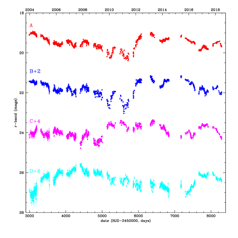
Figure 1: The light curves of the four bright quasar images in SDSS J1004$+$4112. The B, C and D images are offset by 2, 4 and 6 magnitudes, respectively, for display purposes. The data span 14.5 years, from December 20, 2003 until June 21, 2018.

We analyzed all of the Keplercam observations, a total of 797 epochs, including the 88 and 85 epochs already published in Fohlmeister et al. (2007) and Fohlmeister et al. (2008), respectively. For the new analysis we used difference imaging (Alard & Lupton 1998, Alard 2000) light curves with the r-band reference image calibrated using the same 5 stars as in Fohlmeister et al. (2007) and Fohlmeister et al. (2008). For the 173 reprocessed epochs we computed the differences between the new and old values, finding a mean and variance for each quasar image of $\Delta m_{A}=0.096\pm 0.040$, $\Delta m_{B}=0.058\pm 0.058$, $\Delta m_{C}=0.0047\pm 0.062$, and $\Delta m_{D}=-0.10\pm 0.07$ mag. Table 1 gives the final light curves with 1018 epochs after removing epochs where the seeing FWHM was worse than 5″ or there were problems seen in a visual inspection of each image. Fig. 1 shows the final light curves.

3 Results

We measure the time delays using the same basic procedures as in Fohlmeister et al. (2007) and Fohlmeister et al. (2008). We model the quasar light curve by a high order polynomial for the leading image C combined with three additional polynomials for the differences in microlensing between this reference image and each of the other three images. The assumption is that microlensing variability generally occurs on longer time scales (see Mosquera & Kochanek 2011 for the expectations for microlensing time scales) than the intrinsic variability of the quasar, so the microlensing polynomials are lower order than the quasar polynomials. Given a choice of polynomial orders, we can then compute a $\chi^{2}$ goodness of fit of the model to the light curves as a function of the delays. After initial pair wise fits to pin down the delay ranges that needed to be explored, the final fits were to all four images simultaneously, although we do report the results for the pair wise fits. Because we have four images and two long delays, the seasonal gaps are all filled. This avoids a common problem in time delay measurements where the goodness of fit can be improved by using the seasonal gaps to reduce the time period where the light curves overlap. For the final Joint fits we dropped the parts of the C ($JD>2457600$) and D ($JD<2454600$) light curves which will never overlap with the other images. After trimming these data, we are left with $N=3473$ magnitudes to be fit.

To be specific, we model the quasar with a polynomial of order $n=100i+50$ with $i=1$ to $5$ and the microlensing as polynomials of order $m=1$ to $15$. This leads to a family of 75 models. Clearly, picking any particular model would be somewhat arbitrary, so we instead combine all the models using Bayesian methods. Since the models have very different numbers of parameters, we require an information criterion for how models are penalized given their number of parameters $p=n+3m$. We use the Akaike information criterion (AIC), where the penalty added to the log-likelihood ($\ln L=-\chi^{2}/2$) is $p$, and the Bayes information criterion where the penalty is $(p/2)\ln N$ where $N$ is the number of data. The Bayes information criterion (BIC) penalizes new parameters much more heavily since, for $N=3473$, the BIC factor of $(p/2)\ln N=4.08p$ is four times larger than the AIC factor of just $p$. Ideally we will find similar results for both even though they will weight the 75 models very differently. For the pair wise fits, the procedures are the same but there is only one microlensing polynomial instead of three. For the AIC models, the likelihood steadily increases as we increase the polynomial order, while for the BIC models, the maximum likelihood model has $n=350$ and $m=15$. This model has a $\chi^{2}=16839$ for 3078 degrees of freedom. The large $\chi^{2}$ is driven by outliers in the photometric data. It could be reduced eliminating outliers completely or by broadening their uncertainties, but that process always has a degree of arbitrariness. The effect of uniformly broadening the uncertainties to make the $\chi^{2}$ per degree of freedom unity would simply be to broaden the statistical uncertainties by $\sqrt{16839/3078}\sim 2.3$, which would still be less than the dominant uncertainties created by cosmic variance as we explain below.

Table 2 presents the results for all six image combinations, both information criteria (AIC and BIC) and either fitting all 4 light curves simultaneously (Joint) or doing each pair individually (Pair). For the Joint fits, all 6 delay distributions can be directly calculated from the distributions for the three lags actually used as parameters in the fit. The labeling of the delays is that image $i$ lags image $j$ by $\Delta t_{ij}$ where the overall ordering is that C varies first, followed by B, then A and finally D. Figure 2 shows the AIC and BIC probability distributions for the joint fits to the BC, AC and DC delays

Figure 2: Probability distribution functions for the three independent time delays $\Delta t_{BC}$, $\Delta t_{AC}$ and $\Delta t_{DC}$

built from the family of 75 models described in the text for the AIC (solid line) and BIC (dashed line) information criteria.

The results for the four different ways of computing the lags are all in good agreement, albeit not quite to the level of the reported statistical uncertainties. For example, the Joint BC, AC, DC, AB, DA and DB delays differ by $0.6$, $1.7$, $1.4$, $4.0$, $2.1$ and $1.1\sigma$ using the average of the two statistical errors for $\sigma$. The same is roughly true comparing the Joint and Pair results. As seen in Fig. 2, the probability distributions still substantially overlap. Thus, like essentially all other time delay measurements, it would be best to use certainties several times the formal uncertainties to account for systematic uncertainties. At least for the absolute time delays, these uncertainties are irrelevant because of the cosmic variance in time delays due to fluctuations in the matter density along the line of sight. For the models of Bar-Kana (1996), the expected cosmic variance is $\sim 4\%$ or $31$, $33$, $98$, $1.8$, $65$ and $57$ days for the BC through DB delays in Table 2. Even for the short AB delay, cosmic variance is the dominant uncertainty.

Delay ratios are far less affected by cosmic variance. The cosmic variance is due to the fluctuations in the surface density along the line of sight to particular lenses relative to the mean background universe. However, a fluctuation $\kappa_{cv}$ in the convergence, which modifies the individual delays by $1-\kappa_{cv}$, has no effect on a delay ratio because the effects on the two images cancel in a ratio. While SDSS J1004$+$4112 is a large separation lens, it probably is not large enough for gradients in $\kappa_{cv}$ across the lens to matter, so delay ratios are still limited by the statistical and systematic errors in the measurements. Because many of the delays are so long, the fractional uncertainties in some of the delay ratios are tiny. For example $\Delta t_{BC}/\Delta t_{DB}=0.4668\pm 0.0004$ - even if we double or triple the formal uncertainty, the delay ratio is measured to $0.1\%$!

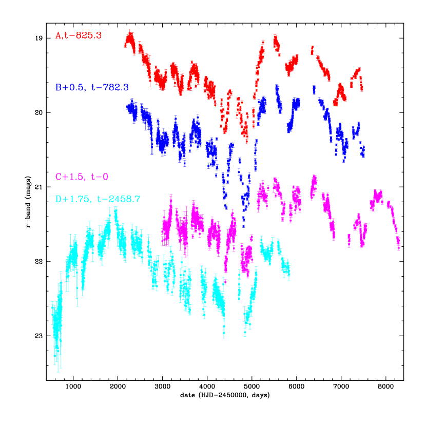
Figure 3: The light curves from Fig. 1 shifted by time delays of 782.3 (B), 825.3 (A) and 2458.7 (D) days with respect to the leading image C. We have added 0.5, 1.5 and 1.75 magnitudes to the B, C and D images, respectively, for display purposes.

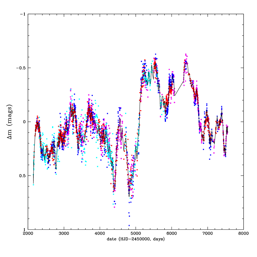
Figure 4: The light curves shifted by the delays and with the microlensing polynomials subtracted. The curve is the polynomial light curve for image C for the $n=350$, $m=15$ model. The images have the same colors as in Figs. 1 and 3 (A red, B blue, C magenta and D cyan). The photometric errors are omitted for clarity.

Fig. 3 shows the four light curves shifted by their $n=350$ and $m=15$ model delays relative to image C ($\Delta t_{BC}^{350.15}=782.3\pm 0.3$ days, $\Delta t_{AC}^{350.15}=825.3\pm 0.3$ days and $\Delta t_{DC}^{350.15}=2458.7\pm 0.6$ days). One can see by eye that there are many large amplitude (compared to the errors) brightness fluctuations that are providing the time delay constraints. In particular, all four light curves contain the sharp rise seen near 5000 days. Fig. 4 shows the light curves shifted by the lags and with the microlensing polynomials subtracted to show how well they overlap. This again emphasizes the large number of coherent variations sampled by multiple images as well as the way the large lags lead to a global light curve with no gaps over the time span where they overlap.

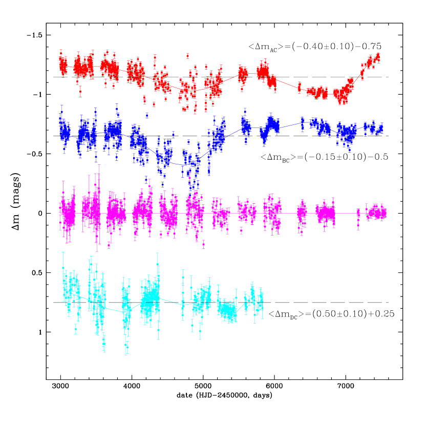
Figure 5: The differential microlensing light curves after subtracting the $n=350$ polynomial model for the light curve of image C. For images A, B and D, the solid curves are the three $m=15$ order polynomials used to model the differential microlensing between these image and C. For image C, the mean residual relative to the light curve model is zero by definition. The time delays have been removed and we only show the period where the light curves overlap and the microlensing signal is well-defined. The images have the same colors as in Figs. 1, 3 and 4 (A red, B blue, C magenta and D cyan). The labels $\langle\Delta m_{DC}\rangle=(0.50\pm 0.10)+0.25$ give the mean magnitude offset, the dispersion of the residuals about the mean and then the shift in magnitude used to improve the visibility of each image.

Fig. 5 shows the differential microlensing of images A, B and D with respect to the reference image of C over the time period when they overlap. The mean magnitude differences between image C and the time shifted images A, B and D are $-0.40\pm 0.10$, $-0.15\pm 0.10$ and $0.50\pm 0.10$, respectively. The errors are the dispersions about the mean rather than the uncertainties in the mean. The differences for A and B are very similar to those measured by Fohlmeister et al. (2008). While there are some coherent short time scale features that may be poorly modeled with intrinsic variability, there are clear, long time scale shifts in the image flux ratios that must be due to microlensing. The little short time scale structure, seen in the residuals, demonstrates that the assumption that we needed a high order polynomial for the source variability but only a low order polynomial for the microlensing model was justified. The amplitude of the microlensing is modest, with a maximum amplitude of roughly $0.5$ mag. It is hard to impute the microlensing effects to particular images – for example, the similarity of the image A and B curves suggests that the microlensing is dominated by image C but the dissimilarity of the image D curve argues against this hypothesis.

4 Discussion and Conclusions

We have measured the last time delay for the four bright images of SDSS J1004+4112. Image D lags image C by 2457 days (6.73 years), the longest measured delay of any gravitational lens. The ability to obtain light curves without seasonal gaps and to flag a sharp variability feature in image C, carry out a reverberation mapping campaign using images A and B and then fill in any missing data with image D makes SDSS J1004+4112 an interesting prospect for such a monitoring campaign. Of the three predictions made after the the measurement of the first two delays by Fohlmeister et al. (2007) and Fohlmeister et al. (2008), the measured delay lies only inside the very broad prediction of 1500 to 2700 days by Mohammed et al. (2015) and is much longer than predicted by Liesenborgs et al. (2009) and Oguri (2010). Oguri (2010) notes that time delay of image D is correlated with the inner slope of the dark matter halo, so it is worthwhile revisiting models for the system.

Time delays have been measured for several other cluster lenses. Fohlmeister et al. (2013) measured a $744\pm 10$ days delay for the two bright quasar images in SDSS J1029$+$2623, the largest separation (22$\farcs$5) quasar lens (Inada et al. 2006). The only detailed model of this system used this delay measurement (Oguri et al. 2013). While SDSS J1029$+$2623 has a third image (Oguri et al. 2008) that could be used as a check of the model, it is faint and close to a brighter image, making it challenging to measure the additional delays. Dahle et al. (2015) measured delays of $47.7\pm 6.0$ days and $722\pm 24$ days between images AB and CA of the six image quasar lens SDSS J2222$+$2745 (Dahle et al. 2013). The models by Dahle et al. (2013) had predicted an AB delay of $-87^{+187}_{-296}$ days and a CA delay of $1399^{+776}_{-850}$ days. Sharon et al. (2017) produced updated models including the first two delay measurements, and it will be interesting to see how well they agree with future measurements. There are also two cluster lenses with lensed supernovae, with measured time delays for one. Predictions (Diego et al. 2016, Jauzac et al. 2016, Oguri 2015, Sharon & Johnson 2015, Zitrin & Broadhurst 2009) for the time delay of supernova “Refsdal” (Kelly et al. 2015) did encompass the eventually measured value (Kelly et al. 2016). However, the predictions also spanned over 400 days and many of the models disagreed in their predictions. It will be interesting to see how well the predictions for the decades long time delays of the second cluster lensed supernova, AT 2016jka (Rodney et al. 2021), hold up.

As in Fohlmeister et al. (2007) and Fohlmeister et al. (2008), we again find that the light curves of the four images are not identical and thus that the images are being microlensed by stars associated with either the cluster galaxies or freely orbiting in the cluster. The differential amplitudes relative to image C are a few tenths of a magnitude, with slow variations over the $\sim 13$ years of overlap. The microlensing was previously used by Fohlmeister et al. (2008) and Fian et al. (2016) to estimate the size of the quasar accretion disk. The effects of microlensing are also seen in the broad emission line profiles (Richards et al. 2004, Gómez-Álvarez et al. 2006, Popović et al. 2020) and the overall wavelength dependence of the quasar flux ratios (Lamer et al. 2006). SDSS J1004+4112 is interesting for microlensing because of the shorter microlensing time scales created by the high dynamical velocities of a cluster (Mosquera & Kochanek 2011) and the prospect of observing microlensing from intracluster stars as opposed to stars associated with the cluster galaxies.

Data Availability Statement

The photometry used in the analysis is included in Table 1.

Table 1: Light curves in r-band magnitude for the four quasar images.

JD-2450000	Image A		Image B		Image C		Image D
2993.523	19.111 $\pm$	0.015	19.421 $\pm$	0.020	20.099 $\pm$	0.038	20.872 $\pm$	0.081
2997.344	19.083 $\pm$	0.021	19.429 $\pm$	0.029	20.229 $\pm$	0.063	20.966 $\pm$	0.132
3022.606	19.044 $\pm$	0.015	19.436 $\pm$	0.021	20.006 $\pm$	0.044	21.143 $\pm$	0.132
3031.920	19.054 $\pm$	0.013	19.476 $\pm$	0.018	20.054 $\pm$	0.037	21.038 $\pm$	0.097
3032.920	19.027 $\pm$	0.013	19.409 $\pm$	0.017	19.990 $\pm$	0.041	21.001 $\pm$	0.109
3033.913	19.020 $\pm$	0.013	19.430 $\pm$	0.017	19.992 $\pm$	0.046	20.996 $\pm$	0.122
3034.916	19.033 $\pm$	0.014	19.459 $\pm$	0.020	20.002 $\pm$	0.034	21.140 $\pm$	0.102
3035.909	19.037 $\pm$	0.013	19.458 $\pm$	0.019	20.070 $\pm$	0.044	21.239 $\pm$	0.133
3037.742	18.984 $\pm$	0.039	19.450 $\pm$	0.060	19.909 $\pm$	0.097	21.194 $\pm$	0.315
3043.854	19.013 $\pm$	0.025	19.452 $\pm$	0.037	20.209 $\pm$	0.078	21.008 $\pm$	0.171

Note. — Table 1 is published in its entirety in the machine-readable format. A portion is shown here for guidance regarding its form and content.

Table 2: Time Delays

Model	Δt_BC	Δt_AC	Δt_DC	Δt_AB	Δt_DA	Δt_DB
	(days)	(days)	(days)	(days)	(days)	(days)
Joint AIC	781.92 ±0.44	825.99 ±0.42	2456.99 ±1.11	44.04 ±0.23	1630.99 ±1.14	1675.06 ±1.14
Joint BIC	782.20 ±0.43	825.23 ±0.46	2458.47 ±1.02	43.01 ±0.27	1633.23 ±0.97	1676.26 ±0.97
Pair AIC	781.14 ±0.34	826.40 ±0.63	2456.62 ±1.15	41.36 ±0.17	1628.75 ±0.87	1675.02 ±2.03
Pair BIC	780.00 ±0.38	827.34 ±0.62	2453.59 ±1.28	43.46 ±0.24	1636.41 ±2.34	1678.20 ±1.63

References

- Alard & Lupton (1998) Alard, C. & Lupton, R. H. 1998, ApJ, 503, 325
- Alard (2000) Alard, C. 2000, A&AS, 144, 363.
- Bar-Kana (1996) Bar-Kana, R. 1996, ApJ, 468, 17
- Dahle et al. (2013) Dahle, H., Gladders, M. D., Sharon, K., et al. 2013, ApJ, 773, 146
- Dahle et al. (2015) Dahle, H., Gladders, M. D., Sharon, K., et al. 2015, ApJ, 813, 67
- Diego et al. (2016) Diego, J. M., Broadhurst, T., Chen, C., et al. 2016, MNRAS, 456, 356
- Fian et al. (2016) Fian, C., Mediavilla, E., Hanslmeier, A., et al. 2016, ApJ, 830, 149
- Fohlmeister et al. (2007) Fohlmeister, J., Kochanek, C. S., Falco, E. E., et al. 2007, ApJ, 662, 62
- Fohlmeister et al. (2008) Fohlmeister, J., Kochanek, C. S., Falco, E. E., et al. 2008, ApJ, 676, 761
- Fohlmeister et al. (2013) Fohlmeister, J., Kochanek, C. S., Falco, E. E., et al. 2013, ApJ, 764, 186
- Gómez-Álvarez et al. (2006) Gómez-Álvarez, P., Mediavilla, E., Muñoz, J. A., et al. 2006, ApJ, 645, L5
- Inada et al. (2003) Inada, N., Oguri, M., Pindor, B., et al. 2003, Nature, 426, 810
- Inada et al. (2005) Inada, N., Oguri, M., Keeton, C. R., et al. 2005, PASJ, 57, L7
- Inada et al. (2008) Inada, N., Oguri, M., Falco, E. E., et al. 2008, PASJ, 60, 27.
- Inada et al. (2006) Inada, N., Oguri, M., Morokuma, T., et al. 2006, ApJ, 653, L97. doi:10.1086/510671
- Jackson (2011) Jackson, N. 2011, ApJ, 739, L28
- Jauzac et al. (2016) Jauzac, M., Richard, J., Limousin, M., et al. 2016, MNRAS, 457, 2029
- Kawano & Oguri (2006) Kawano, Y. & Oguri, M. 2006, PASJ, 58, 271
- Kelly et al. (2015) Kelly, P. L., Rodney, S. A., Treu, T., et al. 2015, Science, 347, 1123
- Kelly et al. (2016) Kelly, P. L., Rodney, S. A., Treu, T., et al. 2016, ApJ, 819, L8
- Lamer et al. (2006) Lamer, G., Schwope, A., Wisotzki, L., et al. 2006, A&A, 454, 493
- Liesenborgs et al. (2009) Liesenborgs, J., de Rijcke, S., Dejonghe, H., et al. 2009, MNRAS, 397, 341
- McKean et al. (2021) McKean, J. P., Luichies, R., Drabent, A., et al. 2021, MNRAS, 505, L36
- Mohammed et al. (2015) Mohammed, I., Saha, P., & Liesenborgs, J. 2015, PASJ, 67, 21
- Mosquera & Kochanek (2011) Mosquera, A. M. & Kochanek, C. S. 2011, ApJ, 738, 96
- Oguri et al. (2004) Oguri, M., Inada, N., Keeton, C. R., et al. 2004, ApJ, 605, 78
- Oguri et al. (2008) Oguri, M., Ofek, E. O., Inada, N., et al. 2008, ApJ, 676, L1
- Oguri (2010) Oguri, M. 2010, PASJ, 62, 1017
- Oguri et al. (2013) Oguri, M., Schrabback, T., Jullo, E., et al. 2013, MNRAS, 429, 482
- Oguri (2015) Oguri, M. 2015, MNRAS, 449, L86
- Ota et al. (2006) Ota, N., Inada, N., Oguri, M., et al. 2006, ApJ, 647, 215
- Popović et al. (2020) Popović, L. Č., Afanasiev, V. L., Moiseev, A., et al. 2020, A&A, 634, A27
- Sharon et al. (2005) Sharon, K., Ofek, E. O., Smith, G. P., et al. 2005, ApJ, 629, L73
- Sharon et al. (2017) Sharon, K., Bayliss, M. B., Dahle, H., et al. 2017, ApJ, 835, 5
- Richards et al. (2004) Richards, G. T., Keeton, C. R., Pindor, B., et al. 2004, ApJ, 610, 679
- Rodney et al. (2021) Rodney, S. A., Brammer, G. B., Pierel, J. D. R., et al. 2021, Nature Astronomy, 5, 1118
- Ross et al. (2009) Ross, N. R., Assef, R. J., Kochanek, C. S., et al. 2009, ApJ, 702, 472
- Sharon & Johnson (2015) Sharon, K. & Johnson, T. L. 2015, ApJ, 800, L26
- Williams & Saha (2004) Williams, L. L. R. & Saha, P. 2004, AJ, 128, 2631
- Zitrin & Broadhurst (2009) Zitrin, A. & Broadhurst, T. 2009, ApJ, 703, L132