Optimal Shelf Arrangement to Minimize Robot Retrieval Time

Abstract

Shelves are commonly used to store objects in homes, stores, and warehouses. We formulate the problem of Optimal Shelf Arrangement (OSA), where the goal is to optimize the arrangement of objects on a shelf for access time given an access frequency and movement cost for each object. We propose OSA-MIP, a mixed-integer program (MIP), show that it finds an optimal solution for OSA under certain conditions, and provide bounds on its suboptimal solutions in general cost settings. We analytically characterize a necessary and sufficient shelf density condition for which there exists an arrangement such that any object can be retrieved without removing objects from the shelf. Experimental data from 1,575 simulated shelf trials and 54 trials with a physical Fetch robot equipped with a pushing blade and suction grasping tool suggest that arranging the objects optimally reduces the expected retrieval cost by 60–80% in fully-observed configurations and reduces the expected search cost by 50–70% while increasing the search success rate by up to 2x in partially-observed configurations. Supplementary material is available at https://sites.google.com/berkeley.edu/osa.

I Introduction

The ability for robots to retrieve target objects quickly from cluttered shelf environments has wide application in automation. When shelves contain heterogeneous objects, the arrangement of objects plays a significant role in retrieval time. For example, if frequent targets are in the front instead of the back, the robot can spend less time moving other objects out of the way to retrieve the target.

Prior work on robot manipulation of objects in shelf-like environments has explored task and motion planning for object rearrangement [1, 2, 3] and the placement of relocated objects during the rearrangement process [4]. This paper considers what makes a good arrangement—specifically, how to arrange objects on a shelf to reduce robot retrieval time. Shelves often contain objects with varying retrieval frequencies and movement costs. For example, in a refrigerator, objects required frequently such as milk should be near the front for easy retrieval. Olive jars and difficult-to-move objects should be near the back to avoid unnecessarily blocking the retrieval of other objects. In this work, we model the retrieval probability and movement cost of each object and formulate the problem of Optimal Shelf Arrangement (OSA): find an arrangement of objects on a shelf that minimizes the expected cost of retrieval.

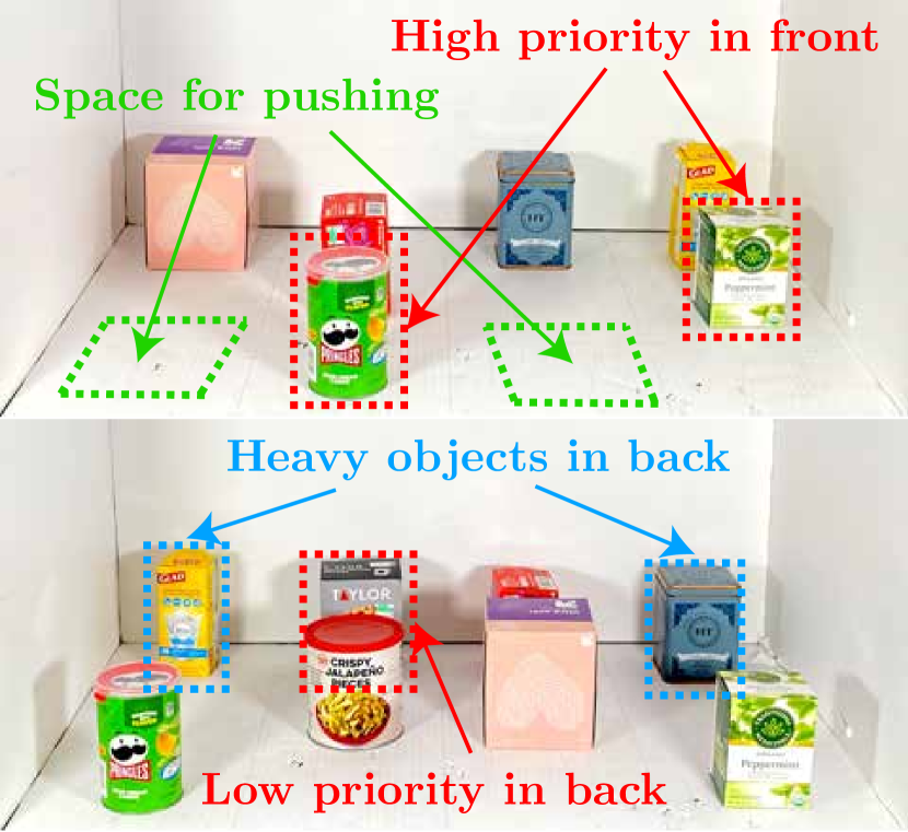
Figure 1: Two optimized shelf arrangements found by OSA-MIP for $n=6$ and $n=8$ objects in a discretized $4\times 3$ shelf. The object cost is proportional to its weight, with heavier objects having higher cost. Green objects have highest priorities, followed by red and yellow objects, with the blue and gray objects having the lowest priority. OSA-MIP trades off priority and moving costs while leaving space between objects to allow pushing actions.

We consider a robot with a combined pushing blade and suction grasping end-effector, or bluction tool [5], that can both push the objects left or right and perform pick-and-place. We assign costs both to each object and to the action type (i.e., the cost is action- and object-specific but path-independent) as in Han et al. [6], where the interpretation of the cost can be the time and effort it takes to relocate each object. The problem is challenging as it requires solving a nested optimization problem: for any arrangement, finding and computing the cost of an optimal action sequence that clears a path to retrieve each target object involves a state-space search itself (see Section III and VII). We bypass this nested optimization and propose OSA-MIP, a mixed-integer program (MIP) that finds a near-optimal solution to the OSA problem. It discretizes the shelf and optimizes the assignment of object locations by minimizing an upper bound on the expected retrieval cost. We characterize situations where the MIP finds an exact optimal solution, and provide bounds on its suboptimality in general cases. We also give a necessary and sufficient shelf-density condition for which there exists an arrangement such that any object can be retrieved without removing objects from the shelf. We also perform simulation experiments exploring how OSA-MIP can change the expected retrieval cost when compared to baselines of Random and Priority-Greedy arrangements.

While the goal of OSA is to optimize object retrieval when the configurations of all objects are known, we conjecture that an optimally-arranged shelf can also speed up object search when their positions are unknown—known as the mechanical search problem [7]. We evaluate OSA-MIP arrangements by comparing the performance of a lateral-access mechanical search policy, SLAX-RAY [5], in both simulated and physical experiments.

This paper makes the following contributions:

1. A formulation of the Optimal Shelf Arrangement (OSA) problem. Given an access frequency and object and action cost, find an arrangement of the objects on the shelf that minimizes expected retrieval cost.

2. A mixed-integer program (MIP) finding an optimal solution to the OSA problem under certain conditions and a suboptimality gap analysis for general cost settings.

3. Simulated experiments with 225 object sets comparing 3 arrangement policies demonstrating a 60 – 80 % reduction in expected one-time retrieval cost and cumulative retrieval cost (full observability case).

4. Simulated and physical experiments comparing 3 arrangement policies suggesting a 2x increase in search success on dense shelves and up to 70 % reduction in the expected search cost (partial observability case).

II Related Work

II-A Storage Assignment Policies

Warehouse layout design and storage assignment policies in automated storage and retrieval systems (AS/RS) are well-studied [8]. Önüt et al. [9] study the optimal warehouse layout design to minimize the total travel distances of the storage rack weighted by the unit handling cost of each item type and the items’ yearly throughput. Hausman et al. [10] compare random, turnover-based, and class-based turnover policies for storage assignment. In particular, turnover-based assignment minimizes the expected one-way travel time [10, 11] and has been extended to multiple command modes and performance measures [12]. Unlike AS/RS systems in which any pallet can be transported by a crane along a rectangular route, objects in a lateral shelf environment can only be accessed when all the obstacles in front of them are cleared. Thus, computing the total expected retrieval cost requires a rearrangement plan to be computed for each target object.

II-B Moving-Block Problems

Motion planning in grid-based storage systems is challenging. One class of widely-studied problems is single-robot motion planning with movable obstacles, represented by the moving-block problems, including the games Sokuban, Pukoban, and Atomix, where a movable block called “the man” tries to move $k$ other movable blocks placed on a grid-square maze into specified target locations through push and/or pull actions. Pereira et al. [13] showed many moving-block problems are NP-hard or PSPACE-complete. Another class is remote motion planning to move a robot from its initial position to a goal position without colliding with obstacles, including the PSPACE-complete game Rush Hour [14] and NP-Hard graph motion planning with one robot (GMP1R) problem [15]. Other related problems include the single-item retrieval planning problem with multiple escorts (SRPME), which seeks to find a multi-robot/item motion plan that brings the requested item to one of the output locations with the minimum total number of item-moves [16], and puzzle-based storage systems [17, 18, 19, 20], where finding the fewest-move solution for a given order is NP-hard [21]. Unlike grid-based storage systems, where all items are routed through conveyors so they can move as long as there is space next to them, in the shelf environment, an item can only be moved when it is accessible by the robot.

II-C Memory Allocation

Finding an optimal arrangement of objects on a shelf for easy retrieval has a similar goal to data and memory allocation for chip multiprocessors, and more specifically, the problem of task scheduling of applications on multiple processors to minimize energy consumption or execution time [22]. Integer programming is a commonly used technique [23, 24, 25, 26]. The OSA-MIP proposed in this work shares similarity with those integer program formulations such as Ozturk et al. [26] where the data access frequencies are considered for memory partitioning when minimizing the overall energy consumption, but the constraints of OSA-MIP focus on clearing obstacles for retrieval instead of partitioning memory components.

II-D Object Rearrangement and Optimal Arrangement

There is a rich literature on manipulation planning among movable obstacles (MAMO) [27]. MAMO is a generalization of the navigation among movable obstacles (NAMO) problem, which is NP-hard [28]. Prior work [1, 29] study the task and motion planning of rearranging multiple objects from one configuration into another using pick-and-place actions on a tabletop. Shome et al. [30, 31] study the multi-arm extension of the problem and formulate mixed integer programs (MIPs) using a graph representation. Cheong et al. [4] focus on the subproblem of where to place relocated objects for object rearrangement. Wang et al. [3] develop a dynamic programming algorithm for uniform cylindrical-shaped objects that minimizes the number of object transfers to rearrange the objects into a goal configuration while avoiding object-object collision. Researchers [32, 33, 34] have also studied the problem of placing objects onto a cluttered surface where existing objects need to first be rearranged to leave space.

Nam et al. [2] develop a task planner to relocate obstacles using lateral pick-and-place actions until a target object becomes reachable in a shelf environment. However, they assume all objects are cylinders graspable from any angle relative to the normal of the shelf back plane. In contrast, we assume the objects can only be accessed along the normal of the shelf back plane, and focus on finding an arrangement optimized for object retrieval instead of the rearrangement motion planning problem with a given target arrangement.

II-E Mechanical Search on Shelves

Mechanical search [35] is the problem of locating and extracting an occluded target object when the arrangement of the objects is partially observable. Gupta et al. [36] interactively explore a cluttered environment until the state of every voxel is known. Dogar et al. [37] propose greedy and $A^{*}$ search algorithms for object search in a cluttered shelf. Lin et al. [38] extend the problem setting to restrict removal of objects from the shelf and additionally consider pushing actions for large ungraspable objects. Recently, Huang et al. [7, 5] proposed a SLAX-RAY search policy that maximizes the reduction in support area of a target object occupancy distribution using a “bluction tool” that combines a pushing blade and a suction cup gripper. In this work, we demonstrate that an optimal shelf arrangement can both increase the search success rate and reduce cost for SLAX-RAY in partially observable simulated and physical mechanical search settings.

III OSA Problem Statement

We consider the Optimal Shelf Arrangement (OSA) problem on a rectangular shelf discretized into a $m_{x}\times m_{y}$ grid with the coordinate frame shown in Figure 2. Given $n$ objects of similar size, a distribution of object retrieval frequencies, and the cost of moving each object, the goal is to find an arrangement that minimizes the expected cost of retrieval. Each object $l$ occupies one cell $(i,j)$, where $i\in\{1,\,\ldots,\,m_{x}\},j\in\{1,\,\ldots,\,m_{y}\}$. We call an object accessible if there are no obstacles in front of it.

As in mechanical search [5], we consider two types of actions: pushing with a planar “blade” ($\mathcal{A}_{p}$) and suction pick-and-place ($\mathcal{A}_{s}$). At each timestep $t$, the robot performs an action $\mathbf{a}_{t}\in\mathcal{A}$ and incurs a cost $c:\mathcal{A}\rightarrow\mathbb{R}_{\geq 0}$, where $\mathcal{A}=\mathcal{A}_{p}\cup\mathcal{A}_{s}$.

1) Pushing actions. Pushing actions in $\mathcal{A}_{p}$, parameterized as $\mathbf{a}_{t}=(i,j,d)$, where $d\in\{-1,1\}$, pushes an object located at $(i,j)$ along the $x$-axis of the shelf frame to $(i+d,j)$. This action is only possible when the object is accessible and pushed to an empty space. We assume there is enough space between objects in neighboring cells to insert the blade and execute the pushing action.

2) Suction actions. Suction actions in $\mathcal{A}_{s}$, parameterized as $\mathbf{a}_{t}=(i,j,i^{\prime},j^{\prime})$, start with the robot forming a seal between the suction cup and object, followed by 3 linear motions: (1) lifting, (2) translating the object along the $x$- and $y$-axes to column $i^{\prime}$, row $j^{\prime}$, and (3) placing the object at its final position $(i^{\prime},j^{\prime})$. This action is only possible if the object to be suctioned is accessible, the target position is empty, and there are no objects in front of the target position.

3) Removal actions. When there are no available placement positions on the shelf, a suction action $\mathbf{a}_{t}=(i,j,-1,$ $-1)\in\mathcal{A}_{s}$ may place the object outside the shelf. The robot incurs a penalty for removing an object from the shelf, as it results in more planning and execution time to move the robot base to access buffer spaces outside the shelf [4].

OSA requires the following parameters:

• $p_{l}$: a probability distribution for requesting object $l$;

• $c_{lp}$: the cost of moving object $l$ with a pushing action;

• $c_{ls}$: the cost of moving object $l$ with a suction action;

• $c_{r}$: the penalty for removing an object from the shelf.

Let $\Delta c_{l}=c_{ls}-c_{lp}$, and $\Delta c_{l}\geq 0~{}\forall l$. We assume $\Delta c_{l}\geq 0$ because suction actions are more prone to failures such as suction seal loss than pushing actions and because prior work [5] empirically found that suction pick-and-place actions take approximately 1.3 times longer than pushing actions. Thus, we set $c_{ls}=1.3c_{lp}$ in our simulated and physical experiments, but the OSA problem and the proposed OSA-MIP (Section V) allow general $c_{lp}$ and $c_{ls}$ values.

Given an arrangement $\mathcal{S}:[1..n]\rightarrow[1..m_{x}]\times[1..m_{y}]$, we let $\mathbf{A}_{l}^{\mathcal{S}}=\{\mathbf{a}_{1}^{\mathcal{S}}(l),...,\mathbf{a}_{t_{l}}^{\mathcal{S}}(l)\}$ denote an optimal sequence of actions to retrieve target object $l$ such that all obstacles in front of $l$ have been cleared and the total cost of the action sequence $\mathrm{cost}(l^{\mathcal{S}})=\sum_{i=1}^{t_{l}}c(\mathbf{a}_{i}^{\mathcal{S}}(l))$ is minimized. The final retrieval action is not included in $\mathbf{A}_{l}^{\mathcal{S}}$ since its cost is the same for all configurations. The cost of an arrangement $\mathcal{S}$ is the expected cost of retrieval among all objects: $C(\mathcal{S})=\mathbb{E}_{l\sim p_{l}}[\text{cost}(l^{\mathcal{S}})]$. The goal is to find an arrangement $\mathcal{S}^{*}=\operatorname*{arg\,min}_{\mathcal{S}}C(\mathcal{S})$ that minimizes the expected cost of retrieval.

IV Shelf Density Analysis

We define the density of a shelf as $\rho:=\frac{n}{m_{x}m_{y}}$. A shelf is dense if $\rho>1-\frac{1}{m_{x}}+\frac{1}{m_{x}m_{y}}$. In Theorem 1, we show that when the density exceeds this threshold, removal is unavoidable for retrieving objects at the back of the shelf. For a square shelf ($m_{x}=m_{y}$), this threshold is at least $\min_{m>0}(1-\frac{1}{m}+\frac{1}{m^{2}})=0.75$. An arrangement $\mathcal{S}$ is hollow if there exists an empty cell behind an occupied cell, and such empty cell is called a cavity. The consolidation process pushes all objects as far back as possible to remove all cavities from a hollow arrangement, and we denote the resulting configuration $\mathcal{S}_{\mathrm{consol}}$.

Theorem 1

There exists an arrangement that does not require removal of objects to retrieve any target if and only if the shelf is not dense.

Proof:

First, we observe that for any retrieval target, a hollow arrangement will never reduce the number of removals required compared to its consolidated version. This is because if $k$ objects are in front of the target and need to be relocated, no removal is required if and only if the total number of empty cells in other columns is at least $k$; if some empty cells are cavities, then one may need to first consolidate the arrangement so that these empty cells are in the front of the shelf to be available to place relocated obstacles. Thus, for any $m_{x}\times m_{y}$ cell, to calculate the maximum number of objects that can fit onto the shelf without requiring removal for retrieving any objects, we only need to consider consolidated arrangements.

Suppose the back $m_{y}-k$ rows are full, and there are $r$ objects in the first $k$ rows. We only need to make sure the backmost object can be successfully retrieved without requiring any removal in each column. Consider any column and assume it has $m_{y}-k+u$ objects. In order to retrieve the backmost object, we need to relocate $m_{y}-k+u-1$ objects into the other columns, which has space equals $k(m_{x}-1)-(r-u)$ cells. So no removal is required if and only if

$$k(m_{x}-1)-(r-u)\geq m_{y}-k+u-1,$$

which simplifies to $k\geq\frac{m_{y}+r-1}{m_{x}}$. By plugging $k$ into density $\rho=\frac{\left(m_{y}-k\right)m_{x}+r}{m_{x}m_{y}}$, we get $\rho\leq\frac{\left(m_{y}-\frac{m_{y}+r-1}{m_{x}}\right)m_{x}+r}{m_{x}m_{y}}=1-\frac{1}{m_{x}}+\frac{1}{m_{x}m_{y}}$. Any denser shelf would not have an arrangement that avoids removal for all target objects. ∎

V MIP Formulation

We propose a mixed-integer program (MIP) to solve OSA and analyze its optimality in Section VI. By assumption, to retrieve a target object, all obstacles in front of it must be relocated. For each obstacle to be moved, all objects in front of it must be cleared by pushing or suction actions. As we assume $c_{ls}\geq c_{lp}~{}\forall l$, pushing actions are preferred over suction. Given these observations, we formulate the MIP as:
Indices:

• $l\in\{1,\,\dots,\,n\}$: object index;

• $i\in\{1,\,\dots,\,m_{x}\}$: x position of the grid;

• $j\in\{1,\,\dots,\,m_{y}\}$: y position of the grid.

Exogenous parameters:

• $p_{l},c_{lp},c_{ls},c_{r}$: retrieval frequency and moving costs for object $l$.

Decision variables:

• $\in\{0,1\}$: indicates if object $l$ is at $(i,j)$;

• $\geq 0$: cost of retrieving object $l$ from $(i,j)$, without including removal penalties;

• $\in\{0,1\}$: indicates if cell $(i,j)$ is occupied;

• $\in\{0,\,\ldots,\,m_{y}\}$: the number of objects in front of and including cell $(i,j)$;

• $\in\{0,1\}$: indicates if all cells in front of and including $(i,j)$ are empty;

• $\in\{0,\,\ldots,\,m_{y}\}$: the number of empty cells at the front of column $i$;

• $\in\{0,1\}$: indicates if either $(i-1,j)$ or $(i+1,j)$ are open (i.e., pushes are available);

• $\delta^{s}_{lij}\in\{0,1\}$: indicates if object $l$ is at $(i,j)$ and can be pushed or can only be suctioned, respectively;

• $\in\{0,1\}$: indicates if there is an object at $(i,j)$ that can be pushed behind another object;

• $\in\{0,\,\ldots,\,m_{y}-1\}$: the number of objects that must be removed from the shelf to retrieve object $l$ from $(i,j)$.

Objective:

Minimize $$\sum_{l=1}^{n}\sum_{i=1}^{m_{x}}\sum_{j=1}^{m_{y}}p_{l}(y_{lij}+c_{r}b_{lij})$$ (1)

The objective (1) minimizes the retrieval cost $y_{lij}$ for each object $l$ (which depends on $c_{lp}$ and $c_{ls}$) plus any removal penalty incurred, weighted by object $l$’s retrieval frequency $p_{l}$. We show in Section VI that this quantity is an upper bound on the true expected cost $C(\mathcal{S})$.
Constraints:

$$\sum_{i=1}^{m_{x}}\sum_{j=1}^{m_{y}}x_{lij}=1, \forall l$$ (2)

$$a_{ij}=\sum_{l=1}^{n}x_{lij}\leq 1 \forall i,j$$ (3)

$$\delta_{ij}=\neg\left(a_{i-1,j}\land a_{i+1,j}\right), \forall i,j$$

$$\delta^{p}_{lij}=x_{lij}\land\delta_{ij},\quad\delta^{s}_{lij}=x_{lij},\land\neg\delta_{ij} \forall l,i,j$$

$$e_{ij}=\sum_{j^{\prime}=1}^{j}a_{ij^{\prime}},\quad f_{ij}=\mathds{1}\left(e_{ij}=0\right), \forall i,j$$

$$d_{i}=\sum_{j=1}^{m_{y}}f_{ij}, \forall i$$

$$y_{lij}= \begin{cases}\leavevmode\resizebox{216.81pt}{}{$\sum_{l^{\prime}\neq l}\sum_{j^{\prime}=1}^{j-1}[c_{l^{\prime}p}\delta^{p}_{l^{\prime}ij^{\prime}}+c_{l^{\prime}s}\delta^{s}_{l^{\prime}ij^{\prime}}]$}&\text{if }x_{lij}=1,\\ 0&\text{if }x_{lij}=0,\end{cases} \forall l,i,j$$

$$\tilde{\delta}_{ij}= a_{ij}\land\neg\left(\left(a_{i-1,j}\lor f_{i-1,j}\right)\land\left(a_{i+1,j}\lor f_{i+1,j}\right)\right) \forall i,j$$

$$b_{lij}= \begin{cases}\leavevmode\resizebox{346.89731pt}{}{$\max{\left(e_{ij}-x_{lij}-\sum_{j^{\prime}=1}^{j-1}\tilde{\delta}_{ij^{\prime}}-\sum_{i^{\prime}\neq i}d_{i^{\prime}},0\right)}$}&\text{if }x_{lij}=1,\\ 0&\text{if }x_{lij}=0,\\ \end{cases} \forall l,i,j$$

$$x_{lij},f_{ij},\delta_{ij},\delta^{p}_{lij},\delta^{s}_{lij},\tilde{\delta}_{ij},a_{ij}\in\{0,1\},\quad \forall l,i,j,$$

$$y_{lij}\in\mathbb{R}_{\geq 0},b_{lij},d_{i},e_{ij}\in\mathbb{Z}_{\geq 0},\quad \forall l,i,j.$$

Constraints (2) and (3) ensure that each object has exactly 1 position and that each position has at most 1 object. All other constraints formally define the decision variables described above. All of the switch-case constraints can be linearized by introducing auxiliary variables; a fully expanded formulation is included in the Appendix. By Theorem 1, if the shelf is not dense, then an arrangement that does not require objects to be removed for retrieval of any target object is possible. In this case, we can add a constraint $\sum_{l=1}^{n}\sum_{i=1}^{m_{x}}\sum_{j=1}^{m_{y}}p_{l}b_{lij}\leq 0$ in place of a large $c_{r}$.

VI Analysis of OSA-MIP

In this section, we analyze the optimality of OSA-MIP’s solutions. Because the retrieval cost depends not only on the total number of actions but also on each object acted on, finding an optimal action sequence $\mathbf{A}_{l}^{\mathcal{S}}$ to retrieve each object requires a state-space search in the general cost settings (see Section VII). Preemptive actions that first rearrange the available shelf space, instead of only relocating obstacles in front of the target, may end up being cheaper even if they require more action steps. However, finding an optimal arrangement $\mathcal{S}^{*}=\operatorname*{arg\,min}_{\mathcal{S}}\mathbb{E}_{l\sim p_{l}}[\text{cost}(l^{\mathcal{S}})]$ where each inner cost computation requires solving a tree-search subproblem for every target object can be intractable.

OSA-MIP computes an upper bound for the optimal retrieval cost for each object and minimizes that upper bound. Formally, we call an action sequence $\mathbf{A}_{l}^{\mathcal{S}}$ non-preemptive if it only involves relocating obstacles in front of the target object $l$, and preemptive otherwise. Let $\hat{\text{cost}}(l^{\mathcal{S}})$ be the optimal cost of retrieving target object $l$ and $\hat{C}(\mathcal{S})=\mathbb{E}_{l\sim p_{l}}[\hat{\text{cost}}(l^{\mathcal{S}})]$ be the corresponding expected retrieval cost when only non-preemptive actions are allowed. Then, as OSA-MIP only considers non-preemptive actions for tractability, it optimizes for $\hat{C}(\mathcal{S})$ instead of $C(\mathcal{S})$, with $\hat{C}(\mathcal{S})\geq C(\mathcal{S})~{}\forall\mathcal{S}$, and may obtain a suboptimal solution $\mathcal{S}_{MIP}$ when $\mathcal{\hat{C}(S}_{MIP})<\mathcal{\hat{C}(S^{*}})$ but $\mathcal{C(S}_{MIP})>\mathcal{C(S^{*})}$, where $\mathcal{S^{*}}$ is an optimal arrangement.

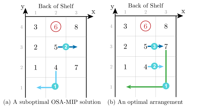
Figure 2: (a) An example where OSA-MIP finds a suboptimal arrangement for retrieving object 6 if $\Delta c_{4}\leq c_{7s}\leq\Delta c_{5}$ and $(p_{5}+p_{6})\Delta c_{4}>p_{6}c_{7s}$ and (b) an optimal arrangement resulting in a lower cost retrieval despite more actions. In (b), the optimal action sequence is to suction object 7 so that object 5 can then be pushed. As OSA-MIP does not consider preemptive actions, it instead leaves a cavity at (3,3) to push object 5.

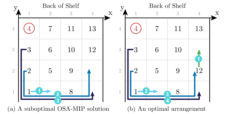
Figure 3: Another example of (a) a suboptimal OSA-MIP solution and (b) an optimal arrangement. To retrieve object 4, the optimal action sequence is to suction object 12 backward to make space for relocating objects 1-3. As OSA-MIP does not consider preemptive actions, it will place object 12 at (4,3) to avoid removing objects if $c_{r}$ is large. However, this arrangement is suboptimal if $p_{4}+p_{7}$ and $p_{10}$ are small compared to $p_{11}$ and $\Delta c_{10}>\Delta c_{9}$.

Figure 2 illustrates an example where OSA-MIP may find a suboptimal solution. In particular, if object 7 has a small suction cost, it may be cheaper to retrieve object 6 in arrangement (2b) than (2a) even though it takes one more action, as illustrated by the arrows in Figure 2. However, as OSA-MIP does not consider preemptive actions (the green arrow) and will use a pushing action on object 4 and a suction action on object 5, it overestimates the retrieval costs for arrangement (2b). It can be shown that if $p_{6}(\Delta c_{5}-\Delta c_{4})>p_{5}\Delta c_{4}>p_{6}(c_{7s}-\Delta c_{4})$, OSA-MIP will suboptimally find (2a) even though (2b) is optimal.

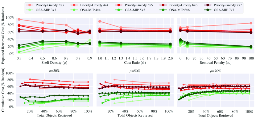
Figure 4: (Top row) Effect of shelf density $\rho$ (left), cost ratio $\psi$ (middle), and removal penalty $c_{r}$ (right) on the cost of OSA-MIP and Priority-Greedy arrangements as a percentage of random arrangement costs across shelf sizes. (Bottom row) Cumulative retrieval cost for OSA-MIP and Priority-Greedy arrangements as a percentage of random arrangement costs for the sequential retrieval task across different shelf densities. OSA-MIP outperfoms baselines despite optimizing only for a single retrieval; however, for denser shelves or as more objects are retrieved, the relative benefit of an OSA-MIP arrangement decreases.

Additionally, OSA-MIP may also produce suboptimal consolidated arrangements to avoid removal when in fact hollow arrangements are optimal, as shown in Figure 3. The arrangement in Figure 3b does not require removal, but to retrieve object 4 or 7, object 12 must be pushed backward to make space for relocating objects 1-3 or 5-6, respectively. As OSA-MIP does not consider this backward push, it will think arrangement (3b) requires removal and overestimate its cost, and it will put object 12 at (4,3) position to avoid removing objects, as shown in Figure 3a even though (3b) can be optimal as it enables pushing object 10. The Appendix contains a full cost analysis of Figures 2 and 3.

However, in cases where the cost saving for pushing compared to suctioning is the same for all objects and preemptive actions are not beneficial, OSA-MIP will be exact, as the following theorem states.

Theorem 2

If $c_{ls}-c_{lp}\equiv\Delta c\leq\min_{l}c_{lp}\text{ }\forall l$, then OSA-MIP finds an optimal solution.

Proof:

When $c_{ls}-c_{lp}\equiv\Delta c\text{ }\forall l$ is a constant, cavity locations are irrelevant (e.g., Figures 2a and 2b are equivalent). If $\Delta c\leq\min_{l}c_{lp}$, preemptive actions to rearrange the space are not beneficial because each preemptive action creates at most one space and 1 suction action is cheaper than 2 pushing actions. Therefore, OSA-MIP’s cost is exact and it will produce an optimal solution. ∎

Theorem 3

Let $\mathcal{S^{*}}$ be an optimal arrangement and $\mathcal{S}_{MIP}$ be an arrangement found by OSA-MIP. Then

$$\mathcal{C(S^{*})} \leq\mathcal{C(S}_{MIP})$$ (4)

$$\leq\min\left\{\mathcal{\hat{C}(S}^{*}_{consol}),\mathcal{\hat{C}(S^{*})}\right\}$$ (5)

$$\leq\min\left\{k\mathcal{C(S^{*})},\mathcal{\hat{C}(S^{*})}\right\},$$ (6)

where $k=\max_{l}\{\frac{c_{ls}}{c_{lp}}\}$.

Proof:

We always have $\mathcal{C(S^{*})}\leq\mathcal{C(S}_{MIP})\leq\mathcal{\hat{C}(S}_{MIP})\leq\min\left\{\mathcal{\hat{C}(S}^{*}_{consol}),\mathcal{\hat{C}(S^{*})}\right\}$, where the last inequality follows from OSA-MIP optimizing $\mathcal{\hat{C}}(.)$.

To show $\mathcal{\hat{C}(S}^{*}_{consol})\leq k\mathcal{C(S^{*})}$, let $\mathcal{\bar{C}(S)}$ be the expected retrieval cost for arrangement $\mathcal{S}$ if we increase $c_{lp}$ to be $c_{ls}~{}\forall l$ and keep $c_{r}$ the same. As argued in Theorem 2, when $c_{lp}=c_{ls}~{}\forall l$, preeemptive actions have no benefit. Thus, $\mathcal{\hat{C}(S}^{*}_{consol})\leq\mathcal{\bar{C}(S}^{*}_{consol})=\mathcal{\bar{C}(S}^{*})\leq k\mathcal{C(S^{*})}$, where the equality is because when pushing and suction costs are equal, the cost of retrieving each object $l$, $\text{cost}(l^{\mathcal{S}})$, is simply the cost of relocating (or removing if necessary) all obstacles in front of $l$, which is equal to $\text{cost}(l^{\mathcal{S}_{consol}})$ for all $\mathcal{S}$. ∎

VII OSA-MIP Planning Experiments

We conduct simulated experiments to evaluate the benefit of OSA-MIP arrangements, as compared to random arrangements or arrangements generated by a priority-greedy algorithm while varying shelf size ($m_{x},m_{y}$), density $\rho$, ratio of suction cost to pushing cost $\psi$, and removal penalty $c_{r}$. Additionally, we evaluate OSA-MIP’s ability to generate arrangements for the sequential retrieval task. We use a Gurobi solver [39] for all of our experiments. For an analysis of OSA-MIP runtime, please refer to the Appendix.

We use 5 shelf sizes $(m_{x},m_{y})\in$ $\{(3,3),$ $(4,4),$ $(5,5),$ $(6,6),$ $(7,7)\}$, 5 density values $\rho\in\{0.3,0.5,0.7,0.8,0.9\}$, 3 cost ratios $\psi\in\{1.0,1.3,2.0\}$, and 3 removal penalties $c_{r}\in\{0,10,100\}$. We sample 3 pushing costs $c_{lp}$ for each object from a discrete uniform distribution on $\{1,\,\ldots,\,10\}$ and let retrieval frequency be inversely proportional to priority (i.e., the probability of being retrieved is $n:(n-1):...:2:1$ for $n$ objects). We compare OSA-MIP to two baseline arrangement algorithms on each of the $5\times 5\times 3\times 3\times 3=675$ object configurations:

1. Random: objects are assigned to a position on the shelf drawn uniformly at random.

2. Priority-Greedy: we select $n$ positions on the shelf uniformly at random, sort the positions by their depth in the shelf, then assign the $n$ objects to the positions in the order of priority (i.e., the highest priority object is assigned to the frontmost position). We use random positions instead of placing all the objects at the front or back of the shelf because the latter approach will not leave space between objects for pushing actions.

To evaluate the true expected cost $C(\mathcal{S})$ for each arrangement, we use an A* search algorithm to find an optimal action sequence $\mathbf{A}_{l}^{\mathcal{S}}$ for retrieving each object and compute the corresponding optimal cost $\text{cost}(l^{\mathcal{S}})$, weighted by the probability $p_{l}$. Preemptive actions are considered: at each step, pushing, suction, and removal actions can be performed on the frontmost object in each column. We use the sum of pushing costs of all obstacles in front of the target object as an admissible heuristic since it is a lower bound on the retrieval cost. However, A* search becomes intractable in relatively dense ($\rho\geq 0.7)$ shelves for target objects at the back both due to the large branching factor and the large number of actions needed to retrieve the object. We switch to a non-preemptive retrieval policy that computes $\hat{\text{cost}}(l^{\mathcal{S}})$ when A* search does not find a solution within 1 minute.

Figure 4 plots the cost of OSA-MIP and Priority-Greedy arrangements as a percentage of Random arrangements for each setting. Since retrieval cost increases as the shelf becomes denser and the number of objects, the suction cost, or the removal penalty increases, we normalize the average cost of OSA-MIP and Priority-Greedy arrangements by that of the Random arrangement. We can see that the expected retrieval cost for OSA-MIP arrangements are 20-40% of the cost of Random arrangements, while Priority-Greedy arrangements have 60-80% of the cost of Random arrangements. As the density increases and the shelf becomes larger, the relative benefit of OSA-MIP decreases slightly but remains nearly half the cost of the Priority-Greedy arrangements. The effect of $\psi$ and $c_{r}$ on the relative cost is small, although OSA-MIP performs relatively better when $c_{r}$ is large because it directly optimizes to avoid removal, unlike Priority-Greedy and Random.

We also evaluate the cumulative cost for sequential object retrieval. We iteratively sample target objects according to the retrieval distribution normalized by the current objects, execute the retrieval, and repeat until all objects have been retrieved or removed. Figure 4 shows the results, which suggest that OSA-MIP has lower cumulative cost, especially for less-dense shelves. As more objects are retrieved and the initial arrangement is disturbed, the relative benefit of OSA-MIP decreases since it optimizes for a single retrieval.

VIII OSA-MIP for Mechanical Search

No.	Metric	Random	Priority-Greedy	OSA-MIP
6	% Visible Objects	61 $\pm$ 15 %	75 $\pm$ 12 %	93 $\pm$ 7 %
	% Success Hidden	100 $\pm$ 0 %	100 $\pm$ 0 %	100 $\pm$ 0 %
	Mean Steps Hidden	1.3 $\pm$ 0.5	1.2 $\pm$ 0.2	1.1 $\pm$ 0.3
	Mean Cost Hidden	10.8 $\pm$ 4.1	10.0 $\pm$ 2.3	6.9 $\pm$ 2.9
8	% Visible Objects	56 $\pm$ 13 %	71 $\pm$ 9 %	81 $\pm$ 7 %
	% Success Hidden	99 $\pm$ 3 %	100 $\pm$ 0 %	100 $\pm$ 0 %
	Mean Steps Hidden	1.5 $\pm$ 0.8	1.3 $\pm$ 0.4	1.2 $\pm$ 0.5
	Mean Cost Hidden	12.5 $\pm$ 7.3	11.5 $\pm$ 4.7	8.1 $\pm$ 2.7
10	% Visible Objects	51 $\pm$ 11 %	67 $\pm$ 7 %	73 $\pm$ 6 %
	% Success Hidden	97 $\pm$ 15 %	97 $\pm$ 15 %	100 $\pm$ 0 %
	Mean Steps Hidden	1.8 $\pm$ 0.7	1.4 $\pm$ 0.4	1.1 $\pm$ 0.4
	Mean Cost Hidden	15.5 $\pm$ 6.4	11.5 $\pm$ 4.1	8.7 $\pm$ 2.9
12	% Visible Objects	41 $\pm$ 8 %	60 $\pm$ 6 %	63 $\pm$ 5 %
	% Success Hidden	85 $\pm$ 33 %	97 $\pm$ 7 %	100 $\pm$ 0 %
	Mean Steps Hidden	1.7 $\pm$ 0.9	1.5 $\pm$ 0.5	1.4 $\pm$ 0.4
	Mean Cost Hidden	14.8 $\pm$ 7.7	13.1 $\pm$ 4.0	10.6 $\pm$ 2.7
14	% Visible Objects	36 $\pm$ 7 %	53 $\pm$ 5 %	55 $\pm$ 7 %
	% Success Hidden	71 $\pm$ 39 %	77 $\pm$ 35 %	100 $\pm$ 0 %
	Mean Steps Hidden	1.7 $\pm$ 1.2	1.3 $\pm$ 0.7	1.7 $\pm$ 0.4
	Mean Cost Hidden	15.2 $\pm$ 10.7	11.5 $\pm$ 6.6	13.4 $\pm$ 3.2
16	% Visible Objects	31 $\pm$ 8 %	51 $\pm$ 5 %	51 $\pm$ 5 %
	% Success Hidden	56 $\pm$ 37 %	59 $\pm$ 39 %	99 $\pm$ 3 %
	Mean Steps Hidden	1.6 $\pm$ 1.3	1.1 $\pm$ 0.9	1.8 $\pm$ 0.4
	Mean Cost Hidden	14.1 $\pm$ 12.1	10.0 $\pm$ 8.1	14.2 $\pm$ 3.7

Table I: Mechanical Search in Sim. Simulation results by SLAX-RAY over 900 trials on a $5\times 4$ discretized shelf across 180 total object configurations. All averages are weighted by the retrieval probabilities of each object. Mean steps and cost are computed among successful searches only. OSA-MIP provides arrangements that lead to the highest proportion of requested targets being visible (i.e., directly retrievable) and achieves the highest search success rate when the target is hidden. The smaller mean steps and cost for baselines in higher density shelves are because SLAX-RAY is only able to find objects in the front rows of those arrangements while it can find objects at the back for OSA-MIP.

While OSA assumes full observability and optimizes for expected retrieval cost, we hypothesize that an optimal arrangement can also benefit lateral-access mechanical search, where a known target object must be searched from a partially observed shelf of unknown objects. We evaluate Random, Priority-Greedy, and OSA-MIP arrangements for mechanical search using SLAX-RAY [5]. SLAX-RAY calculates the target occupancy distribution, which indicates the probability of each object occluding the target object, then greedily reduces the occupancy distribution support through pushing and suction actions using a bluction tool. In contrast to the action set in Section III, removal actions are not considered by SLAX-RAY and objects cannot be moved behind other objects, so we set $c_{r}$ to a large value in OSA-MIP to discourage removal actions. We use a shelf size of $0.8\text{\times}0.5\text{\times}0.5\text{\,}\mathrm{m}$ in both simulation and physical experiments. A trial is successful when the target is retrievable.

VIII-A Simulation Experiments

We conduct experiments in simulation using the First Order Shelf Simulator (FOSS) simulator [7]. We discretize the shelf into a $5\times 4$ grid with 6, 8, 10, 12, 14 or 16 cuboid objects, with each setting repeated 50 times for each arrangement. The objects are generated with random dimensions within the limit of the grid size, and are assigned retrieval probabilities $p_{l}$ drawn from a standard uniform and normalized. As heavier objects tend to be more difficult to move, we set the pushing cost of each object to be proportional to its volume and use a cost ratio of $\psi=1.3$. We evaluate each arrangement based on the number of steps, success rate, and retrieval cost SLAX-RAY produces for each object, weighted by $p_{l}$. SLAX-RAY fails if it takes $2n$ actions without revealing the target object or if there are no allowable actions (e.g., all cells in the front row are occupied).

Table I shows the results. The mean steps and cost are computed only among successful searches. “Visible objects” refer to the case where the target requested is already placed at the front of a column and so is directly retrievable without any steps of search. We see that OSA-MIP arrangements not only have the largest proportion of time when the requested target is readily retrievable, but the search success rate among hidden objects remains 99-100% even for relatively dense shelves, and is 40-43% higher than baselines for 16 objects. The smaller mean steps and cost for baselines in dense shelves are because SLAX-RAY can only successfully find objects in the front rows which has fewer steps, while OSA-MIP leaves sufficient space for SLAX-RAY to manipulate and find deeply-hidden objects at the back so its weighted average steps and cost among all successful trials are larger.

VIII-B Physical Experiments

We use a physical Fetch robot with a “bluction” tool [5] and an Intel RealSense LiDAR Camera L515 for RGBD observations. We discretize the shelf into a $4\times 3$ grid, select a set of 4, 6, or 8 household objects (shown in Figure 1), and assign them a priority order and cost based on their weight. We run the same experiments for each object set as in simulation. Table II shows the results. As the shelf is not dense, SLAX-RAY successfully finds all targets in all arrangements so there is no bias in the means due to the exclusion of failures as in Table I. We see that OSA-MIP achieves 2x fewer steps and 3x lower cost to find hidden objects on average, suggesting that mechanical search policies can benefit from optimally arranged objects. A direct comparison with simulation, where the shelf is discretized into a $4\times 3$ grid, is included in the Appendix.

No.	Metric	Random	Priority-Greedy	OSA-MIP
4	% Visible Objects	63.2 %	78.9 %	100 %
	Mean Steps Hidden	1.0	1.0	0.0
	Mean Cost Hidden	7.0	10.0	0.0
6	% Visible Objects	77.8 %	55.6 %	81.5 %
	Mean Steps Hidden	4.7	2.6	2.2
	Mean Cost Hidden	37.7	20.1	11.2
8	% Visible Objects	50.0 %	69.4 %	69.4 %
	Mean Steps Hidden	5.1	3.1	2.4
	Mean Cost Hidden	29.2	22.6	11.1

Table II: Mechanical Search in Real. Results by SLAX-RAY over 54 trials with a Fetch robot on a physical shelf discretized into a $4\times 3$ grid. As the shelf is not dense, SLAX-RAY finds all targets successfully in all arrangements. All averages are weighted by the objects’ retrieval probabilities. OSA-MIP produces arrangements for which SLAX-RAY can find the target in 2x fewer steps and 3x lower cost than baselines, suggesting that mechanical search policies can benefit from optimally arranging objects for retrieval.

IX Conclusion and Future Work

In this paper, we formalize the Optimal Shelf Arrangement (OSA) problem, and propose OSA-MIP, a mixed-integer program that efficiently optimizes an upper bound of the expected retrieval cost and solves for a near-optimal arrangement. Experiments suggest that optimally arranged shelves achieve significant cost savings compared to randomly and greedily arranged shelves for both object retrieval and search. In future work, we will consider the problem of rearranging the current shelf into a near-optimal arrangement; given an arrangement, instead of completely rearranging the shelf to place the objects in an optimal arrangement, it may be desirable to find a near-optimal arrangement that also minimizes disturbance from the current configuration.

X Appendix

X-A Fully-Linearized MIP Formulation for OSA

In this section, we give the linearized formulation of the proposed MIP:

$$\text{Minimize }\sum_{l=1}^{n}\sum_{i=1}^{m_{x}}\sum_{j=1}^{m_{y}}p_{l}(y_{lij}+c_{r}b_{lij})$$ (7)

$$\text{Subject to }\sum_{i=1}^{m_{x}}\sum_{j=1}^{m_{y}}x_{lij}=1,\quad\forall l$$ (8)

$$a_{ij}=\sum_{l=1}^{n}x_{lij}\leq 1,\quad\forall i,j$$ (9)

$$\delta_{ij}\leq M\left(2-(a_{i-1,j}+a_{i+1,j})\right)\quad\forall i,j$$ (10)

$$\delta^{p}_{lij}\leq x_{lij}\quad\forall l,i,j$$ (11)

$$\delta^{p}_{lij}\leq\delta_{ij}\quad\forall l,i,j$$ (12)

$$\delta^{p}_{lij}\geq x_{lij}+\delta_{ij}-1\quad\forall l,i,j$$ (13)

$$\delta^{s}_{lij}\leq x_{lij}\quad\forall l,i,j$$ (14)

$$\delta^{s}_{lij}\leq 1-\delta_{lij}\quad\forall l,i,j$$ (15)

$$\delta^{s}_{lij}\geq x_{lij}-\delta_{lij}\quad\forall l,i,j$$ (16)

$$\sum_{l^{\prime}\neq l}\sum_{j^{\prime}=1}^{j-1}\left[c_{l^{\prime}p}\delta^{p}_{l^{\prime}ij^{\prime}}+c_{l^{\prime}s}\delta^{s}_{l^{\prime}ij^{\prime}}\right]-y_{lij}\leq Mz_{lij}\quad\forall l,i,j$$ (17)

$$x_{lij}\leq 1-z_{lij},\quad\forall i,j$$ (18)

$$e_{ij}=\sum_{j^{\prime}=1}^{j}a_{ij^{\prime}},\quad\forall i,j$$ (19)

$$e_{ij}\leq M(1-f_{ij})\quad\forall i,j$$ (20)

$$d_{i}=\sum_{j=1}^{m_{y}}f_{ij},\quad\forall i$$ (21)

$$\tilde{\delta}_{ij}\leq a_{ij},\quad\forall i,j$$ (22)

$$\tilde{\delta}_{ij}\leq g_{ij},\quad\forall i,j$$ (23)

$$\tilde{\delta}_{ij}\geq a_{ij}+g_{ij}-1,\quad\forall i,j$$ (24)

$$1-h_{ij}\geq a_{ij},\quad\forall i,j$$ (25)

$$1-h_{ij}\geq f_{ij},\quad\forall i,j$$ (26)

$$1-h_{ij}\leq a_{ij}+f_{ij},\quad\forall i,j$$ (27)

$$g_{ij}\geq h_{i-1,j},\quad\forall i,j$$ (28)

$$g_{ij}\geq h_{i+1,j},\quad\forall i,j$$ (29)

$$g_{ij}\leq h_{i-1,j}+h_{i+1,j},\quad\forall i,j$$ (30)

$$\bigg{(}e_{ij}-x_{lij}-\sum_{j^{\prime}=1}^{j-1}\tilde{\delta}_{ij^{\prime}}-\sum_{i^{\prime}\neq i}d_{i^{\prime}}\bigg{)}-b_{lij}\leq Mz_{lij}\quad\forall l,i,j$$ (31)

$$x_{lij},z_{lij},f_{ij},g_{ij},h_{ij},\delta_{ij},\delta^{p}_{lij},\delta^{s}_{lij},\tilde{\delta}_{ij}\in\{0,1\},\quad\forall l,i,j,$$ (32)

$$y_{lij}\in\mathbb{R}_{\geq 0},a_{ij},b_{lij},d_{i},e_{ij}\in\mathbb{Z}_{\geq 0},\quad\forall l,i,j.$$ (33)

X-B Analysis of Suboptimality for Figures 2 and 3

In this section, we give a detailed analysis of the condition for the two examples in Section VI where OSA-MIP may find a suboptimal solution.

X-B1 Figure 2

Comparing arrangement (2b) and (2a), the difference lies in the retrieval costs for objects 5 and 6. For retrieving object 5, arrangement (2b) costs $\min(c_{4s},c_{4p}+c_{7s})$ while arrangement (2a) costs only $c_{4p}$. For retrieving object 6, arrangement (2b) costs $\min(c_{4s}+c_{5p},c_{7s}+c_{4p}+c_{5p})$ while arrangement (2a) costs $\min(c_{4p}+c_{5s},c_{7s}+c_{4p}+c_{5p})$. If $\Delta c_{4}\leq c_{7s}$ and $\Delta c_{5}\geq c_{7s}$, then arrangement (2b) costs $\Delta c_{4}$ less for retrieving object 5 but $c_{7s}-\Delta c_{4}$ more for retrieving object 6 compared to arrangement (2a). Considering the retrieval probabilities, if $p_{5}\Delta c_{4}>p_{6}(c_{7s}-\Delta c_{4})$, then arrangement (2b) is more optimal than arrangement (2a).

However, as the OSA-MIP does not consider the possibility of preemptive actions, it overestimates the retrieval costs for arrangement (2b). In particular, for retrieving object 5, it will conclude that arrangement (2b) saves $\Delta c_{4}$, and for retrieving object 6, it will conclude that arrangement (2b) costs $(c_{4p}+c_{5s})-(c_{4s}+c_{5p})=\Delta c_{5}-\Delta c_{4}$ more. Now if $p_{6}(\Delta c_{5}-\Delta c_{4})>p_{5}\Delta c_{4}>p_{6}(c_{7s}-\Delta c_{4})$, OSA-MIP will choose arrangement (2a) over arrangement (2a) even though arrangement (2b) is actually more optimal if preemptive actions are allowed.

X-B2 Figure 3

Let the configuration in Figure 3a be $\mathcal{S}_{A}$, and the configuration in Figure 3b be $\mathcal{S}_{B}$. Then we have

$$\mathcal{C(S}_{A})-\mathcal{C(S}_{B})$$ (34)

$$= (p_{4}+p_{7})(-\min\left\{c_{12,s},c_{r}\right\})$$

$$+p_{10}(c_{9p}-\min\left\{c_{9s},c_{9p}+c_{12,s}\right\})$$

$$+p_{11}\big{(}\min\left\{c_{9p}+c_{10,s},c_{9p}+c_{10,p}+c_{12,s}\right\}$$

$$~{}~{}~{}~{}-\min\left\{c_{9s}+c_{10,p},c_{9p}+c_{10,p}+c_{12,s}\right\}\big{)}$$

and

$$\mathcal{\hat{C}(S}_{A})-\mathcal{\hat{C}(S}_{B})$$ (35)

$$= (p_{4}+p_{7})(-c_{r})+p_{10}(c_{9p}-c_{9s})$$

$$+p_{11}((c_{9p}+c_{10,s})-(c_{9s}+c_{10,p})).$$

When $\mathcal{C(S}_{A})>\mathcal{C(S}_{B})$ but $\mathcal{\hat{C}(S}_{A})<\mathcal{\hat{C}(S}_{B})$, the MIP will choose $\mathcal{S}_{A}$ over $\mathcal{S}_{B}$ while $\mathcal{S}_{B}$ is more optimal than $\mathcal{S}_{A}$ due to preemptive actions.

Since

$$\min\left\{c_{9p}+c_{10,s},c_{9p}+c_{10,p}+c_{12,s}\right\}$$ (36)

$$- \min\left\{c_{9s}+c_{10,p},c_{9p}+c_{10,p}+c_{12,s}\right\}$$

$$= \min\left\{\Delta c_{10}-\Delta c_{9},c_{12,s}-\Delta c_{9}\right\}$$

if both components are nonnegative, we have $\mathcal{C(S}_{A})>\mathcal{C(S}_{B})$ when

$$p_{11}\min\left\{\Delta c_{10}-\Delta c_{9},c_{12,s}-\Delta c_{9}\right\}$$ (37)

$$> (p_{4}+p_{7})\min\left\{c_{12,s},c_{r}\right\}+p_{10}\Delta c_{9},$$

assuming $\Delta c_{10}>\Delta c_{9}$ and $c_{12,s}>\Delta c_{9}$.

On the other hand, $\mathcal{\hat{C}(S}_{A})<\mathcal{\hat{C}(S}_{B})$ is equivalent to

$$\begin{split}p_{11}(\Delta c_{10}-\Delta c_{9})<{}&(p_{4}+p_{7})c_{r}+p_{10}\Delta c_{9}.\end{split}$$ (38)

Therefore, if $\Delta c_{9}<c_{12,s}<c_{r}$, $\Delta c_{9}<\Delta c_{10}$, and $p_{11}$ is sufficiently large compared to $p_{4}+p_{7}$ and $p_{10}$, then it is possible that

$$\begin{split}{}&(p_{4}+p_{7})\min\left\{c_{12,s},c_{r}\right\}+p_{10}\Delta c_{9}\\ <&p_{11}\min\left\{\Delta c_{10}-\Delta c_{9},c_{12,s}-\Delta c_{9}\right\}\\ \leq&p_{11}(\Delta c_{10}-\Delta c_{9})\\ <&(p_{4}+p_{7})c_{r}+p_{10}\Delta c_{9},\end{split}$$ (39)

in which case the OSA-MIP solution will be suboptimal.

X-C Runtime Analysis of OSA-MIP

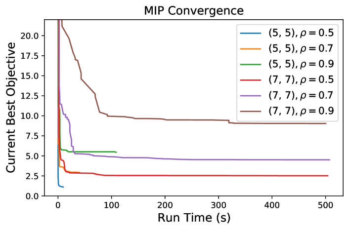
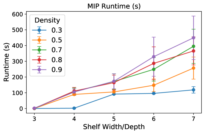
Figure 5: OSA-MIP runtime across shelf sizes and densities. Top: The objective of the best incumbent found during the process of optimization on 6 different problem instances (shelf width = 5 or 7, density = 0.3, 0.7, 0.9). The discontinuation of the lines indicates that a provably optimal solution has been found; otherwise, the optimization is run for 500s. Bottom: The MIP average runtime among the 675 problem instances (see Section VII), grouped by shelf width and density. The MIP is terminated if the best incumbent solution stops improving for 90s.

Figure 5 plots the average computation time of OSA-MIP as a function of shelf size and density. The experiments were conducted using a Gurobi solver [39] on a MacBook Pro with 2.4 GHz 8-Core Intel Core i9 and 32GB memory. The top figure plots the objective of the best incumbent found during the process of optimization on 6 different problem instances (shelf width = 5 or 7, density = 0.3, 0.7, 0.9). The discontinuation of the lines indicates that a provably optimal solution has been found; otherwise, the optimization is run for 500s. We can see that for 5x5 shelves, the solver is able to find an optimal solution within 120s even for 90% density. For 7x7 shelves, the solver is not able to find a provably optimal solution within 500s, but the best objective has converged, indicating that a near-optimal solution has been found. Thus, for the 675 instances described in Section VII, we terminate the optimization if the best incumbent solution stops improving for 90s. The bottom figure plots the MIP average runtime grouped by shelf width and density. Unsurprisingly, the runtime scales with the shelf size and density. For a 7x7 shelf and 90% density, it takes the solver about 8 minutes to find a near-optimal solution.

X-D More SLAX-RAY Simulation Results

No.	Metric	Random	Priority-Greedy	OSA-MIP
4	% Visible Objects	72 $\pm$ 20 %	84 $\pm$ 15 %	100 $\pm$ 0 %
	% Success Hidden	100 $\pm$ 0 %	100 $\pm$ 0 %	- $\pm$ - %
	Mean Steps Hidden	1.0 $\pm$ 0.1	1.0 $\pm$ 0.1	- $\pm$ -
	Mean Cost Hidden	8.6 $\pm$ 2.0	8.7 $\pm$ 1.9	- $\pm$ -
6	% Visible Objects	58 $\pm$ 14 %	76 $\pm$ 10 %	86 $\pm$ 5 %
	% Success Hidden	93 $\pm$ 23 %	99 $\pm$ 5 %	100 $\pm$ 0 %
	Mean Steps Hidden	1.1 $\pm$ 0.4	1.1 $\pm$ 0.3	1.1 $\pm$ 0.5
	Mean Cost Hidden	10.1 $\pm$ 4.3	9.3 $\pm$ 3.6	7.5 $\pm$ 6.3
8	% Visible Objects	48 $\pm$ 11 %	67 $\pm$ 7 %	73 $\pm$ 7 %
	% Success Hidden	83 $\pm$ 30 %	81 $\pm$ 35 %	100 $\pm$ 0 %
	Mean Steps Hidden	1.2 $\pm$ 0.6	1.1 $\pm$ 0.6	1.0 $\pm$ 0.2
	Mean Cost Hidden	10.1 $\pm$ 5.7	8.5 $\pm$ 4.7	7.5 $\pm$ 1.3
10	% Visible Objects	40 $\pm$ 10 %	59 $\pm$ 7 %	60 $\pm$ 7 %
	% Success Hidden	40 $\pm$ 35 %	53 $\pm$ 40 %	98 $\pm$ 4 %
	Mean Steps Hidden	0.6 $\pm$ 0.7	0.7 $\pm$ 0.6	1.2 $\pm$ 0.2
	Mean Cost Hidden	5.1 $\pm$ 6.6	5.7 $\pm$ 5.4	9.2 $\pm$ 2.2

Table III: Mechanical Search in Sim, $4\times 3$ discretization. Simulation results by SLAX-RAY over 600 trials on a $4\times 3$ discretized shelf across 120 total object configurations. All averages are weighted by the retrieval probabilities of each object. Mean steps and cost are computed among successful searches only. OSA-MIP provides arrangements that lead to more objects that are directly visible and a search success rate among hidden objects 45-58% higher than baselines. The smaller mean steps and cost for baselines in higher density shelves are because SLAX-RAY is only able to find objects in the front rows of those arrangements while it can find objects at the back of the shelf for OSA-MIP arrangements.

We show simulation results that use the same $4\times 3$ discretization as in the physical experiments. We discretize the shelf into a $5\times 4$ grid with 4, 6, 8, or 10 cuboid objects, with each setting repeated 50 times for each arrangement. The objects are generated with random dimensions within the limit of the grid size, and are assigned retrieval probabilities $p_{l}$, drawn from a standard uniform distribution and normalized. We set the pushing cost of each object to be proportional to its volume and use a cost ratio of $\psi=1.3$.

Table III shows the results. Similar to Table I, the mean steps and cost are computed only among successful searches. We see that OSA-MIP arrangements not only have the largest proportion of time when the requested target is readily retrievable, but the search success rate among hidden objects remains 98-100% even for relatively dense shelves, and is 45-58% higher than baselines for 10 objects. The smaller mean steps and cost for baselines in dense shelves are because SLAX-RAY can only successfully find objects in the front rows which has fewer steps, while OSA-MIP leaves sufficient space for SLAX-RAY to manipulate and find deeply-hidden objects at the back so its weighted average steps and cost among all successful trials are larger.

References

- [1] A. Krontiris and K. E. Bekris, “Dealing with difficult instances of object rearrangement.” in Proc. Robotics: Science and Systems (RSS), vol. 1123, 2015.
- [2] C. Nam, J. Lee, S. H. Cheong, B. Y. Cho, and C. Kim, “Fast and resilient manipulation planning for target retrieval in clutter,” in Proc. IEEE Int. Conf. Robotics and Automation (ICRA), 2020, pp. 3777–3783.
- [3] R. Wang, K. Gao, D. Nakhimovich, J. Yu, and K. E. Bekris, “Uniform object rearrangement: From complete monotone primitives to efficient non-monotone informed search,” in Proc. IEEE Int. Conf. Robotics and Automation (ICRA), 2021, pp. 6621–6627.
- [4] S. H. Cheong, B. Y. Cho, J. Lee, C. Kim, and C. Nam, “Where to relocate?: Object rearrangement inside cluttered and confined environments for robotic manipulation,” in Proc. IEEE Int. Conf. Robotics and Automation (ICRA), 2020, pp. 7791–7797.
- [5] H. Huang, M. Danielczuk, C. M. Kim, L. Fu, Z. Tam, J. Ichnowski, A. Angelova, B. Ichter, and K. Goldberg, “Mechanical search on shelves using a novel “bluction” tool,” in Proc. IEEE Int. Conf. Robotics and Automation (ICRA), 2022.
- [6] S. D. Han, N. M. Stiffler, K. E. Bekris, and J. Yu, “Efficient, high-quality stack rearrangement,” IEEE Robotics & Automation Letters, vol. 3, no. 3, pp. 1608–1615, 2018.
- [7] H. Huang, M. Dominguez-Kuhne, V. Satish, M. Danielczuk, K. Sanders, J. Ichnowski, A. Lee, A. Angelova, V. Vanhoucke, and K. Goldberg, “Mechanical search on shelves using lateral access x-ray,” in Proc. IEEE/RSJ Int. Conf. on Intelligent Robots and Systems (IROS), 2021, pp. 2045–2052.
- [8] J. Karásek, “An overview of warehouse optimization,” Int. Journal of Advances in Telecommunications, Electrotechnics, Signals and Systems, vol. 2, no. 3, pp. 111–117, 2013.
- [9] S. Önüt, U. R. Tuzkaya, and B. Doğaç, “A particle swarm optimization algorithm for the multiple-level warehouse layout design problem,” Computers & Industrial Engineering, vol. 54, no. 4, pp. 783–799, 2008.
- [10] W. H. Hausman, L. B. Schwarz, and S. C. Graves, “Optimal storage assignment in automatic warehousing systems,” Management science, vol. 22, no. 6, pp. 629–638, 1976.
- [11] U. W. Thonemann and M. L. Brandeau, “Note. optimal storage assignment policies for automated storage and retrieval systems with stochastic demands,” Management Science, vol. 44, no. 1, pp. 142–148, 1998.
- [12] M. E. Johnson and M. L. Brandeau, “Stochastic modeling for automated material handling system design and control,” Transportation science, vol. 30, no. 4, pp. 330–350, 1996.
- [13] A. G. Pereira, L. S. Buriol, and M. Ritt, “Solving moving-blocks problems,” in Anais do XXX Concurso de Teses e Dissertações, 2017.
- [14] G. W. Flake and E. B. Baum, “Rush hour is pspace-complete, or “why you should generously tip parking lot attendants”,” Theoretical Computer Science, vol. 270, no. 1-2, pp. 895–911, 2002.
- [15] C. H. Papadimitriou, P. Raghavan, M. Sudan, and H. Tamaki, “Motion planning on a graph,” in Proc. Symposium on Foundations of Computer Science, 1994, pp. 511–520.
- [16] A. Yalcin, “Multi-agent route planning in grid-based storage systems,” Ph.D. dissertation, Europa-Universität Viadrina Frankfurt, 2018.
- [17] K. R. Gue and B. S. Kim, “Puzzle-based storage systems,” Naval Research Logistics (NRL), vol. 54, no. 5, pp. 556–567, 2007.
- [18] V. R. Kota, D. Taylor, and K. R. Gue, “Retrieval time performance in puzzle-based storage systems,” Journal of Manufacturing Technology Management, 2015.
- [19] K. R. Gue, K. Furmans, Z. Seibold, and O. Uludağ, “Gridstore: a puzzle-based storage system with decentralized control,” IEEE Trans. Automation Science and Engineering, vol. 11, no. 2, pp. 429–438, 2013.
- [20] M. Mirzaei, R. B. De Koster, and N. Zaerpour, “Modelling load retrievals in puzzle-based storage systems,” Int. Journal of Production Research, vol. 55, no. 21, pp. 6423–6435, 2017.
- [21] D. Ratner and M. K. Warmuth, “Finding a shortest solution for the n n extension of the 15-puzzle is intractable.” in Association for the Advancement of Artificial Intelligence (AAAI), 1986, pp. 168–172.
- [22] H. Salamy and J. Ramanujam, “An effective solution to task scheduling and memory partitioning for multiprocessor system-on-chip,” IEEE Trans. Computer-Aided Design of Integrated Circuits and Systems, vol. 31, no. 5, pp. 717–725, 2012.
- [23] R. Niemann and P. Marwedel, “Hardware/software partitioning using integer programming,” in Design, Automation and Test in Europe (DATE) Conference, 1996, pp. 473–479.
- [24] S.-R. Kuang, C.-Y. Chen, and R.-Z. Liao, “Partitioning and pipelined scheduling of embedded system using integer linear programming,” in Int. Conf. on Parallel and Distributed Systems (ICPADS), vol. 2, 2005, pp. 37–41.
- [25] O. Avissar, R. Barua, and D. Stewart, “An optimal memory allocation scheme for scratch-pad-based embedded systems,” ACM Trans. Embedded Computing Systems (TECS), vol. 1, no. 1, pp. 6–26, 2002.
- [26] O. Ozturk, G. Chen, M. Kandemir, and M. Karakoy, “An integer linear programming based approach to simultaneous memory space partitioning and data allocation for chip multiprocessors,” in IEEE Computer Society Annual Symposium on Emerging VLSI Technologies and Architectures (ISVLSI), 2006, pp. 6–pp.
- [27] M. Stilman, J.-U. Schamburek, J. Kuffner, and T. Asfour, “Manipulation planning among movable obstacles,” in Proc. IEEE Int. Conf. Robotics and Automation (ICRA), 2007, pp. 3327–3332.
- [28] M. Stilman and J. J. Kuffner, “Navigation among movable obstacles: Real-time reasoning in complex environments,” Int. Journal of Humanoid Robotics, vol. 2, no. 04, pp. 479–503, 2005.
- [29] S. D. Han, N. M. Stiffler, A. Krontiris, K. E. Bekris, and J. Yu, “High-quality tabletop rearrangement with overhand grasps: Hardness results and fast methods,” in Proc. Robotics: Science and Systems (RSS), 2017.
- [30] R. Shome, K. Solovey, J. Yu, K. Bekris, and D. Halperin, “Fast, high-quality two-arm rearrangement in synchronous, monotone tabletop setups,” IEEE Trans. Automation Science and Engineering, vol. 18, no. 3, pp. 888–901, 2021.
- [31] R. Shome and K. E. Bekris, “Synchronized multi-arm rearrangement guided by mode graphs with capacity constraints,” in Workshop on the Algorithmic Foundation of Robotics (WAFR), 2020, pp. 243–260.
- [32] A. Cosgun, T. Hermans, V. Emeli, and M. Stilman, “Push planning for object placement on cluttered table surfaces,” in Proc. IEEE/RSJ Int. Conf. on Intelligent Robots and Systems (IROS), 2011, pp. 4627–4632.
- [33] G. Havur, G. Ozbilgin, E. Erdem, and V. Patoglu, “Geometric rearrangement of multiple movable objects on cluttered surfaces: A hybrid reasoning approach,” in Proc. IEEE Int. Conf. Robotics and Automation (ICRA), 2014, pp. 445–452.
- [34] A. R. Dabbour, “Placement generation and hybrid planning for robotic rearrangement on cluttered surfaces,” Ph.D. dissertation, Sabancı University, 2019.
- [35] M. Danielczuk, A. Kurenkov, A. Balakrishna, M. Matl, D. Wang, R. Martín-Martín, A. Garg, S. Savarese, and K. Goldberg, “Mechanical search: Multi-step retrieval of a target object occluded by clutter,” in Proc. IEEE Int. Conf. Robotics and Automation (ICRA), 2019, pp. 1614–1621.
- [36] M. Gupta, T. Rühr, M. Beetz, and G. S. Sukhatme, “Interactive environment exploration in clutter,” in Proc. IEEE/RSJ Int. Conf. on Intelligent Robots and Systems (IROS), 2013, pp. 5265–5272.
- [37] M. R. Dogar, M. C. Koval, A. Tallavajhula, and S. S. Srinivasa, “Object search by manipulation,” Autonomous Robots, vol. 36, no. 1, pp. 153–167, 2014.
- [38] Y.-C. Lin, S.-T. Wei, S.-A. Yang, and L.-C. Fu, “Planning on searching occluded target object with a mobile robot manipulator,” in Proc. IEEE Int. Conf. Robotics and Automation (ICRA), 2015, pp. 3110–3115.
- [39] Gurobi Optimization, LLC, “Gurobi Optimizer Reference Manual,” 2022. [Online]. Available: https://www.gurobi.com