Enhanced superconductivity through virtual tunneling in Bernal bilayer graphene coupled to WSe₂

Abstract

Motivated by a recent experiment [arXiv:2205.05087], we investigate a possible mechanism that enhances superconductivity in hole-doped Bernal bilayer graphene due to a proximate WSe₂ monolayer. We show that the virtual tunneling between WSe₂ and Bernal bilayer graphene, which is known to induce Ising spin-orbit coupling, can generate an additional attraction between two holes, providing a potential explanation for enhancing superconductivity in Bernal bilayer graphene. Using microscopic interlayer tunneling, we derive the Ising spin-orbit coupling and the effective attraction as functions of the twist angle between Bernal bilayer graphene and the WSe₂ monolayer. Our theory provides an intuitive and physical explanation for the intertwined relation between Ising spin-orbit coupling and superconductivity enhancement, which should motivate future studies.

Introduction.— Recent experiments on Bernal bilayer graphene (BBG) Zhou et al. (2022) and rhombohedral trilayer graphene (RTG) Zhou et al. (2021a) reveal multiple symmetry broken phases and provide a new understanding for superconductivity in general graphene systems (i.e., moiré Cao et al. (2018); Yankowitz et al. (2019); Lu et al. (2019); Hao et al. (2021); Park et al. (2021a); Cao et al. (2021); Liu et al. (2021); Zhang et al. (2021); Park et al. (2021b); Burg et al. (2022); Siriviboon et al. (2021) or moiréless systems Zhou et al. (2021a, 2022); Zhang et al. (2022)). In these non-moiré crystalline graphene multilayers, superconducting states with $T_{c}\leq 0.1$K are found in narrow regions close to interaction-driven “isospin” polarized phases Zhou et al. (2021b, a, 2022). Theoretically, the acoustic-phonon-mediated pairing can provide a consistent resolution for superconductivity in BBG and RTG Chou et al. (2021a, 2022a, 2022b), while interaction-driven mechanisms are also proposed Chatterjee et al. (2021); Ghazaryan et al. (2021); Dong and Levitov (2021); Cea et al. (2022); Szabó and Roy (2022a); You and Vishwanath (2022); Qin et al. (2022); Dai et al. (2022); Szabó and Roy (2022b); Dong et al. (2022).

A new experiment on superconductivity in BBG demonstrates that superconductivity can be significantly enhanced with a proximate WSe₂ Zhang et al. (2022). The system consists of a WSe₂ monolayer on top of a BBG, and a displacement field ($D$) is used to control the layer-polarization of the low-energy bands. For a sufficiently large $D>0$, the carriers of hole-doped BBG reside entirely on the top layer, and superconductivity is observed around $0.3$K without a magnetic field. The superconducting state shows a nontrivial response to an in-plane magnetic field – a Pauli-limit violation at lower doping and Pauli-limited behavior at higher doping. For $D<0$, no superconductivity is observed for $T\geq 30$mK, but the normal states are essentially consistent with the previous experiment without a WSe₂ layer Zhou et al. (2022). The strikingly different results for $D>0$ and $D<0$ suggest the significance of the proximate WSe₂ layer. It is important to emphasize that WSe₂ enhances superconductivity quite substantially – the superconducting temperature is enhanced by an order of magnitude (from 30mK to 300mK), the region of the superconducting phase also becomes wider, and an in-plane magnetic field is no longer required to induce superconductivity.

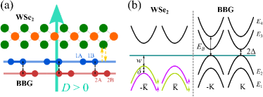
Figure 1: Setup of BBG-WSe₂ and band structure. (a) Side view of the BBG-WSe₂ system. The WSe₂ monolayer is on top of the BBG. A displacement field along the $z$-direction is exerted. (b) The schematic band structures of WSe₂ and BBG. The green line indicates the Fermi energy, which is on the band edge of the first BBG valence band ($E_{2}$). We ignore the spin splitting of the WSe₂ conduction bands in this illustration. We use $E_{1}$, $E_{2}$, $E_{3}$, and $E_{4}$ to label the BBG bands in ascending order in energy.

The key task is to identify the physical origin of superconductivity enhancement. Since a small observable $T_{c}$ has been found in BBG Zhou et al. (2022), any additional pairing glue or reduction of Coulomb repulsion can result in a noticeable enhancement in superconductivity. However, such a cooperative enhancing mechanism must be absent without a nearby WSe₂ layer, manifesting an asymmetric effect in $D>0$ and $D<0$. The main goal of the current work is to provide a potential explanation for the WSe₂-enhanced superconductivity in BBG Zhang et al. (2022).

In this Letter, we propose a novel mechanism that enhances pairings in a BBG-WSe₂ system based on the interlayer tunneling between WSe₂ and BBG. Such a tunneling process is believed to induce Ising spin-orbit coupling (ISOC) in BBG Island et al. (2019); Zhang et al. (2022); Gmitra et al. (2016); Gmitra and Fabian (2017); Khoo et al. (2017), implying significant interlayer tunneling. We develop a minimal theory that produces an effective attraction between two holes in the slightly hole-doped BBG via a virtual interlayer tunneling process in combination with an interaction between hole carriers and the virtual electron. Furthermore, we derive the ISOC and effective attraction as functions of the relative angle between WSe₂ and BBG, incorporating microscopic tunneling at extended Brillouin zones Bistritzer and MacDonald (2010); David et al. (2019). Our results suggest that the enhanced superconductivity can be explained by the virtual tunneling from the WSe₂ layer in cooperation with the electron-phonon interaction, paving the way for higher-$T_{c}$ superconducting states in graphene systems.

Model.— We are interested in a BBG-WSe₂ system as depicted in Fig. 1. In the presence of a sufficiently large displacement field along $z$-direction ($D>0$), the low-energy valence band of BBG is polarized at the 1A site [illustrated in Fig. 1(a)] on the top graphene layer. It was shown theoretically Gmitra and Fabian (2017); Khoo et al. (2017) and experimentally Island et al. (2019); Zhang et al. (2022) that ISOC is induced primarily on the layer proximate to WSe₂, suggesting that tunneling between WSe₂ and the top graphene layer is essential. Thus, a minimal model must include certain properties of WSe₂ and BBG bands as well as the interlayer tunneling between WSe₂ and the top layer of BBG.

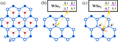
Figure 2: Lattice model and virtual tunneling processes. (a) The effective honeycomb lattice model for BBG. A sites (blue dots) and B sites (blue opened circles) correspond to the positions of 1A and 1B sites in Fig. 1(a), respectively; the red dots indicate the 2B sites in the bottom graphene layer; 2A sites are right below the 1B sites. (b) ISOC due to virtual tunneling. (c) Attraction due to virtual tunneling.

To simplify the problem, we consider an effective honeycomb model as follows (see Fig. 2 and SM ):

$$\hat{H}_{\text{tG}}=E_{A}\sum_{\bm{\mathrm{r}}_{A}}n(\bm{\mathrm{r}}_{A})+E_{B}\sum_{\bm{\mathrm{r}}_{B}}n(\bm{\mathrm{r}}_{B}),$$ (1)

where $E_{A}$ ($E_{B}$) corresponds to the onsite energy of the effective A (B) sites, $n(\bm{\mathrm{r}}_{\sigma})=\sum_{\tau,s}c^{\dagger}_{\tau\sigma s}(\bm{\mathrm{r}}_{\sigma})c_{\tau\sigma s}(\bm{\mathrm{r}}_{\sigma})$ is the number operator at site $\bm{\mathrm{r}}_{\sigma}$, $c_{\tau\sigma s}$ is the fermionic annihilation operator with valley $\tau K$, sublattice $\sigma=A,B$, and spin $s$. The lack of hopping is because we consider momentum right at $K$ or $-K$, where the system can be viewed as a collection of decoupled atomic sites. Equation (1) is a simplified description of BBG degrees of freedom relevant to the virtual tunneling processes considered in this work, and we retain only the $E_{2}$ band (A sites) and the $E_{4}$ band (B sites), where the $E_{2}$ and $E_{4}$ bands are labeled in Fig. 1(b). Due to the interlayer dimerization between 1B and 2A sites, the microscopic 1B sites of BBG are associated with both the $E_{1}$ and $E_{4}$ bands. For our proposal, the $E_{4}$ band is important, while the $E_{1}$ band is ignored. Thus, we consider $E_{A}=0$ and set the value of $E_{B}$ to the energy difference between the $E_{4}$ and the $E_{2}$ band edges EB , as illustrated in Fig. 1(b). In such a model, the charge neutral configuration [i.e., $\mathcal{E}_{F}$ is inside the $2\Delta$ gap of Fig. 1(b)] corresponds to a state with completely filled A sites and empty B sites. In our case with $\mathcal{E}_{F}$ at the $E_{2}$ band edge, the system is slightly hole-doped, and we can consider ground states with dilute holes on the A sites of the effective honeycomb lattice model [given by Eq. (1)]. Again, the effective description here is valid when $\mathcal{E}_{F}$ is at the $E_{2}$ band edge.

In addition to the onsite potential, we consider electron-electron interactions given by

$$\hat{H}_{I}\!=\!\frac{U_{0}}{2}\sum_{\bm{\mathrm{r}}}\delta n(\bm{\mathrm{r}})\left[\delta n(\bm{\mathrm{r}})\!-\!1\right]\!+\!U_{1}\!\!\!\!\sum_{\langle\bm{\mathrm{r}}_{A},\bm{\mathrm{r}}_{B}\rangle}\!\!\!\!\delta n(\bm{\mathrm{r}}_{A})\delta n(\bm{\mathrm{r}}_{B}),$$ (2)

where $\delta n(\bm{\mathrm{r}})=n(\bm{\mathrm{r}})-\langle 0|n(\bm{\mathrm{r}})|0\rangle$, $|0\rangle$ is the state with a charge neutral configuration (i.e., filled $A$ sites and empty $B$ sites), $U_{0}>0$ ($U_{1}>0$) is the onsite (nearest-neighbor) Coulomb interaction, and $\langle\bm{\mathrm{r}}_{A},\bm{\mathrm{r}}_{B}\rangle$ denotes the nearest-neighbor pair. We consider a sufficiently large $U_{0}$ such that at most one hole (electrons) can be created on sublattice A (B). The $U_{1}$ term describes the interaction between nearest-neighbor sites, and $U_{1}<E_{B}$ is assumed (as the spontaneous formation of dipoles is forbidden). We will focus on the electron-hole attraction betweenan electron on the B site and a hole on the nearest-neighbor A site in the virtual process.

The WSe₂ layer can be described by a semiconductor bandstructure with spin split valence bands Xiao et al. (2012) as illustrated in Fig. 1(b). Specifically, the energy splittings can be described by an ISOC, $\lambda\tau_{z}s_{z}$, with $\tau_{z}$ ($s_{z}$) being the $z$-component Pauli matrix for valley (spin). The interlayer tunneling between WSe₂ and BBG can facilitate spin-orbit splitting in BBG valence bands. To provide an intuitive understanding, we treat WSe₂ valence bands as a few representative energy levels described by a simplified Hamiltonian,

$$\hat{H}_{d}\!=\!-\!W\!\!\left(d_{+,\uparrow}^{\dagger}d_{+,\uparrow}\!+\!d_{-,\downarrow}^{\dagger}d_{-,\downarrow}\right)\!-\!(W+\delta)\!\!\left(d_{-,\uparrow}^{\dagger}d_{-,\uparrow}\!+\!d_{+,\downarrow}^{\dagger}d_{+,\downarrow}\right)\!,$$ (3)

where $d_{\tau,s}$ denotes the fermionic annihilation operator with valley $\tau\bar{K}$ and spin $s$ in the WSe₂ valence bands. $W$ and $\delta$ are the parameters for the WSe₂ valence bands.

Finally, we consider a tunneling Hamiltonian between WSe₂ and BBG given by

$$\hat{H}_{V}\!=\!\! \sum_{\tau,s,\bm{\mathrm{r}}_{A}}\!\!\left\{c^{\dagger}_{\tau As}(\bm{\mathrm{r}}_{A})\left[V^{A}_{\tau s}d_{\tau,s}+\bar{V}^{A}_{\tau s}d_{-\tau,s}\right]\!+\text{H.c.}\right\}$$

$$+\!\!\sum_{\tau,s,\bm{\mathrm{r}}_{B}}\!\!\left\{c^{\dagger}_{\tau Bs}(\bm{\mathrm{r}}_{B})\left[V^{B}_{\tau s}d_{\tau,s}\!+\!\bar{V}^{B}_{\tau s}d_{-\tau,s}\right]\!+\text{H.c.}\right\}\!,$$ (4)

where $V^{\sigma}_{\tau s}$ is the tunneling strength for the intravalley process (i.e., $\tau\bar{K}$ to $\tau K$), and $\bar{V}^{\sigma}_{\tau s}$ is the tunneling strength for the intervalley process (i.e., $-\tau\bar{K}$ to $\tau K$) Tun . Since the entire system preserves the (spinful) time-reversal symmetry, the tunneling terms obey $\left|V^{\sigma}_{\bar{\tau}\bar{s}}\right|=\left|V^{\sigma}_{\tau s}\right|$ and $\left|\bar{V}^{\sigma}_{\bar{\tau}\bar{s}}\right|=\left|\bar{V}^{\sigma}_{\tau s}\right|$, where $\bar{\tau}$ ($\bar{s}$) means the time-reversal partner of $\tau$ ($s$).

The model designed here is physically motivated for understanding ISOC and effective attraction via interlayer tunneling. However, such a simplified model cannot capture the full microscopic detail. We will later use a detailed approach incorporating WSe₂ band structures and the microscopic interlayer tunneling matrix elements.

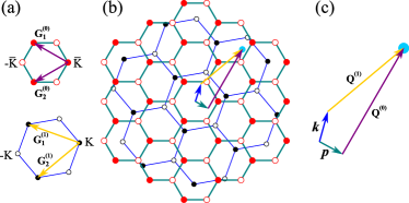
Figure 3: Brillouin zone and geometry of interlayer tunneling. (a) First Brillouin zone of WSe₂ (green) and BBG (blue). BBG is rotated by a twist angle $\theta$. We use $\theta=10^{\circ}$ here. $\bm{\mathrm{G}}^{(0)}_{a}$’s and $\bm{\mathrm{G}}^{(1)}_{a}$’s are the primitive lattice vectors of a reciprocal lattice of WSe₂ and BBG, respectively. (b) Extended Brillouin zones. (c) Momenta $\bm{\mathrm{p}}$ and $\bm{\mathrm{k}}$ have the same crystal momentum as $\bm{\mathrm{p}}+\bm{\mathrm{Q}}^{(0)}=\bm{\mathrm{k}}+\bm{\mathrm{Q}}^{(1)}$, where $\bm{\mathrm{Q}}^{(0)}$ and $\bm{\mathrm{Q}}^{(1)}$ are the reciprocal lattice vectors of WSe₂ and BBG, respectively.

Ising spin-orbit coupling and effective attraction.— The minimal model $\hat{H}=\hat{H}_{\text{tG}}+\hat{H}_{I}+\hat{H}_{d}+\hat{H}_{V}$ [given by Eqs. (1), (2), (3), and (Enhanced superconductivity through virtual tunneling in Bernal bilayer graphene coupled to WSe₂)] can straightforwardly produce ISOC in the first valence band of BBG. The main idea is that the second-order perturbation in $\hat{H}_{V}$ as sketched in Fig. 2(b) (see also SM ) generates spin-valley-splitting energy levels on the A sites, realizing an ISOC with strength

$$\lambda_{I}= \frac{\left|V^{A}_{+\uparrow}\right|^{2}-\left|\bar{V}^{A}_{+\uparrow}\right|^{2}}{W}-\frac{\left|V^{A}_{+\downarrow}\right|^{2}-\left|\bar{V}^{A}_{+\downarrow}\right|^{2}}{W+\delta}.$$ (5)

The main goal of this work is to investigate if the interlayer tunneling between WSe₂ and BBG can generate an effective attractive interaction. Specifically, we consider two holes that contain a common nearest-neighbor B site at $\bm{\mathrm{x}}_{B}$ as illustrated in Fig. 2(c). At the second-order perturbation of $\hat{H}_{V}$, the interplay between virtual tunneling and the interaction $\hat{H}_{I}$ [Eq. (2)] generates an effective attraction between the holes, described by SM

$$\hat{H}_{\text{att}}=-\mathcal{U}_{\text{eff}}\sum_{\langle\langle\bm{\mathrm{r}}_{A},\bm{\mathrm{r}}_{A}^{\prime}\rangle\rangle}\delta n(\bm{\mathrm{r}}_{A})\delta n(\bm{\mathrm{r}}_{A}^{\prime}),$$ (6)

where the sum runs over the nearby pairs on A sites and

$$\mathcal{U}_{\text{eff}}\!= \frac{\mathcal{V}^{2}_{\uparrow}}{W+E_{B}}+\frac{\mathcal{V}^{2}_{\uparrow}}{W+E_{B}-2U_{1}}-\frac{2\mathcal{V}^{2}_{\uparrow}}{W+E_{B}-U_{1}}$$

$$\!+\!\frac{\mathcal{V}^{2}_{\downarrow}}{W+\delta+E_{B}}\!+\!\frac{\mathcal{V}^{2}_{\downarrow}}{W+\delta+E_{B}-2U_{1}}\!-\!\frac{2\mathcal{V}^{2}_{\downarrow}}{W+\delta+E_{B}-U_{1}}$$ (7)

with $\mathcal{V}^{2}_{s}=2\left|V^{B}_{+s}\right|^{2}+2\left|\bar{V}^{B}_{+s}\right|^{2}$. $\mathcal{U}_{\text{eff}}$ vanishes as $U_{1}$ is absent. While the electron on a B site has a large local energy $E_{B}$, the nearest-neighbor electron-hole attraction can lower the total energy in a virtual state. In Eq. (Enhanced superconductivity through virtual tunneling in Bernal bilayer graphene coupled to WSe₂), those terms with $-2U_{1}$, corresponding to virtual tunneling to $\bm{\mathrm{x}}_{B}$, yield the dominant contributions as long as $U_{1}>0$. We assume that $W+E_{B}>2U_{1}$ so that the any charge transfer between WSe₂ and BBG should be absent. Since $|V^{A}_{\tau s}|$ and $|V^{B}_{\tau s}|$ are of the same order of magnitude SM , we expect that the virtual tunneling generates a sizable effective attraction $\mathcal{U}_{\text{eff}}$. Our theory therefore provides an intuitive understanding of the effective attraction due to a proximate WSe₂ layer.

The proposed mechanism here is conceptually related to the “polarizer” idea Little (1964); Hamo et al. (2016) and the repulsion-induced attraction in models on the honeycomb lattice Slagle and Fu (2020); Crépel and Fu (2021, 2022); Crépel et al. (2022). We discuss a few differences between our work and Refs. Slagle and Fu (2020); Crépel and Fu (2021, 2022); Crépel et al. (2022) – (i) The virtual process is due to interlayer tunneling rather than intralayer hopping, and (ii) the electron-hole attraction in the virtual process rather than electron-electron repulsion. Point (i) is crucial as our mechanism describes a possible enhanced attraction from WSe₂ rather than pairings due to intralayer processes. In addition, point (ii) allows for a wider parameter range for a sizable effective attraction because the large onsite energy $E_{B}$ can be compensated by a nearest neighbor attraction.

Interlayer tunneling and twist angle.— The interlayer tunneling between WSe₂ and BBG crucially determines ISOC as well as the virtual-tunneling-induced effective attraction. The interlayer tunneling preserves crystal momentum as the matrix element primarily depends on the distance between the sites. Within the two-center approximation scheme, the tunneling between the layers can be described by Bistritzer and MacDonald (2010)

$$T_{\bm{\mathrm{k}},\bm{\mathrm{p}}}^{\alpha,\sigma;\beta,\sigma^{\prime}}= \frac{1}{\sqrt{\mathcal{A}_{0}\mathcal{A}_{1}}}\left(a^{(1)}_{\bm{\mathrm{k}},\alpha,\sigma}\right)^{*}\left(a^{(0)}_{\bm{\mathrm{p}},\beta,\sigma^{\prime}}\right)\times$$

$$\!\!\sum_{\bm{\mathrm{Q}}^{(1)},\bm{\mathrm{Q}}^{(0)}}\!\!\tilde{t}_{\bm{\mathrm{k}}+\bm{\mathrm{Q}}^{(1)}}e^{i\phi^{\sigma;\sigma^{\prime}}_{\bm{\mathrm{Q}}^{(1)},\bm{\mathrm{Q}}^{(0)}}}\delta_{\bm{\mathrm{k}}+\bm{\mathrm{Q}}^{(1)},\bm{\mathrm{p}}+\bm{\mathrm{Q}}^{(0)}},$$ (8)

where $\mathcal{A}_{0}$ ($\mathcal{A}_{1}$) is the unit-cell area of WSe₂ (BBG), $\alpha$ and $\beta$ are the band indexes, $\bm{\mathrm{k}}$ of BBG and $\bm{\mathrm{p}}$ of WSe₂ are the momentum relative to $\Gamma$ point (Brillouin zone center), $\sigma$ and $\sigma^{\prime}$ are the sublattice (orbital) indexes, $a^{(l)}_{\bm{\mathrm{k}},\alpha,\sigma}$ is the sublattice (orbital) projection of a Bloch state $|\bm{\mathrm{k}},\alpha\rangle$ at layer $l$, $\bm{\mathrm{Q}}^{(0)}$, $\bm{\mathrm{Q}}^{(1)}$ are the reciprocal lattice vectors in WSe₂ and BBG, respectively, and $\phi^{\sigma;\sigma^{\prime}}_{\bm{\mathrm{Q}}^{(1)},\bm{\mathrm{Q}}^{(0)}}$ is a phase factor depending on sublattice. In the above expression, we use index $0$ for the WSe₂ layer and index $1$ for the top graphene layer of BBG. $\tilde{t}_{\bm{\mathrm{k}}}$ is the 2D Fourier transform of the interlayer tunneling amplitude with a finite range, and we use a stretched exponential ansatz form Bistritzer and MacDonald (2010),

$$|\tilde{t}_{\bm{\mathrm{k}}}|=t_{0}e^{-\chi\left(|\bm{\mathrm{k}}|z_{\perp}\right)^{\gamma}},$$ (9)

where $t_{0}$ is an overall constant, $\chi$ is an order 1 numerical constant, $\gamma$ is the exponent of the stretched exponential, and $z_{\perp}$ is the distance between the WSe₂ monolayer and the top graphene layer of BBG zpe . Note that Eq. (9) is an empirical expression for a finite $\bm{\mathrm{k}}$, and the potential complications for $\bm{\mathrm{k}}\rightarrow 0$ are not relevant to our problem.

The interlayer tunneling described by Eq. (8) is a highly nontrivial single-particle process. Microscopically, WSe₂ and BBG have a relative angle that is tunable experimentally as well as different lattice constants ($d=3.31\text{\AA}$ for WSe₂, $a=2.46\text{\AA}$ for BBG), resulting in Brillouin zones illustrated in Fig. 3. Note that $T_{\bm{\mathrm{k}},\bm{\mathrm{p}}}^{\alpha,\sigma;\beta,\sigma^{\prime}}$ is nonzero as long as $\bm{\mathrm{k}}+\bm{\mathrm{Q}}^{(1)}=\bm{\mathrm{p}}+\bm{\mathrm{Q}}^{(0)}$ for some reciprocal lattice vectors $\bm{\mathrm{Q}}^{(0)}$ and $\bm{\mathrm{Q}}^{(1)}$. Thus, a full calculation must incorporate a sufficiently large number of extended Brillouin zones. Using the virtual-tunneling ideas discussed previously, we can compute the $\lambda_{I}$ and $\mathcal{U}_{\text{eff}}$ incorporating the microscopic interlayer tunneling matrix elements between the $\bm{\mathrm{k}}\cdot\bm{\mathrm{p}}$ WSe₂ bands Xiao et al. (2012) and our honeycomb model. We summarize the main results, and the complete derivations are provided in SM .

In Fig. 4, we plot the twist-angle ($\theta$) dependence of $\lambda_{I}$ with a few representative values of $\chi$ and $\gamma$ par . $\lambda_{I}$ is generally positive for small positive $\theta$ and becomes negative slightly above $\theta=15^{\circ}$. Moreover, nonmonotonic behavior can manifest near $\theta=5^{\circ}$ and $\theta=20^{\circ}$ for smaller $\gamma$ and $\chi$. These results can be understood by the geometry of momentum at $\theta=5^{\circ}$ and $\theta\geq 20^{\circ}$ SM . At $\theta=30^{\circ}$, $\lambda_{I}$ vanishes because the intervalley and intravalley tunnelings have exactly the same contributions. Similar nonmonotonic behavior near $\theta=20^{\circ}$ was also theoretically reported in graphene coupled to transition metal dichalcogenide David et al. (2019); Li and Koshino (2019); Naimer et al. (2021). In addition, the sign changing in $\lambda_{I}$ (curves with $\gamma=1$ in Fig. 4) was also obtained in Ref. David et al. (2019). In Fig. 5, we plot the $\theta$ dependence of $\mathcal{U}_{\text{eff}}$ with $U_{1}=0.3$eV and $U_{1}=0.43$eV (the largest possible value in our theory) and a few different values of $\chi$ and $\gamma$. $\mathcal{U}_{\text{eff}}$ is generally larger at smaller $\theta$, but nonmonotonic features might develop for small $\gamma$ and $\chi$. While the qualitative results are insensitive to $U_{1}$, the quantitative values depend on $U_{1}$ SM . An important implication here is that ISOC strength and the effective attraction are not directly related to each other. The full results depend a lot on the details of $T_{\bm{\mathrm{k}},\bm{\mathrm{p}}}^{\alpha,\sigma;\beta,\sigma^{\prime}}$.

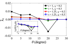
Figure 4: Ising spin-orbit coupling versus twist angle ($\theta$) with microscopic interlayer tunneling. We plot the dimensionless spin-orbit coupling $\tilde{\lambda}_{I}=\lambda_{I}\mathcal{A}_{0}\mathcal{A}_{1}\text{eV}/t_{0}^{2}$ as a function of $\theta$ with different values of $\gamma$ and $\chi$. $W=0.62$eV and $\delta=0.46$eV for all the plots.

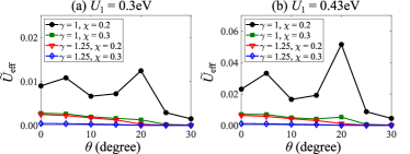
Figure 5: Effective attraction versus twist angle ($\theta$) with microscopic interlayer tunneling. We plot the dimensionless spin-orbit coupling $\tilde{U}_{\text{eff}}=\mathcal{U}_{\text{eff}}\mathcal{A}_{0}\mathcal{A}_{1}\text{eV}/t_{0}^{2}$ as a function of $\theta$ with different values of $\gamma$, $\chi$, and $U_{1}$. (a) $U_{1}=0.3$eV. (b) $U_{1}=0.43$eV. $W=0.62$eV and $\delta=0.46$eV for all the plots.

Discussion.— The virtual-tunneling-induced attraction might explain the enhanced superconductivity in BBG-WSe₂ Zhang et al. (2022) as it enters the theory nonperturbatively in an exponential function determining $T_{c}$ and the effect is primarily on $D>0$. In the BBG experiment without WSe₂ Zhou et al. (2022), superconductivity with $T_{c}\sim 30$mK was reported at the doping density $n_{e}=-6\times 10^{12}$cm^-2 with a Fermi-surface degeneracy factor of 2, implying that the pairing interaction between holes overcomes Coulomb suppression. Since the enhanced superconductivity is found near the same doping density with a very similar Fermi-surface degeneracy factor, we anticipate that the same pairing mechanism manifests in BBG with or without the proximate WSe₂. According to Ref. Chou et al. (2022a), the acoustic-phonon-mediated attraction is slightly stronger than the Coulomb suppression, so any additional pairing glue due to presence of the WSe₂, albeit small compared to the Coulomb repulsion, might considerably enhance superconductivity because $T_{c}$ is exponentially related to the coupling constant. As such, our theory based on the interplay between virtual tunneling and interaction is a possible explanation for the BBG-WSe₂ experiment Zhang et al. (2022). We also derive the twist-angle dependence of the ISOC parameter and the effective attraction, providing guidance for future BBG-WSe₂ systems.

It is worth mentioning that our theory most likely underestimates $\mathcal{U}_{\text{eff}}$ because we consider only the nearest-neighbor Coulomb interaction and only valley momenta (i.e., $K$ and $-K$ points) in the BBG bands. With a long-range Coulomb interaction, a long-range effective attraction can also arise from virtual tunneling processes, resulting in an overall stronger pairing. Moreover, incorporating all the allowed momenta in the BBG $E_{4}$ band also enhances $\mathcal{U}_{\text{eff}}$ because there are more states to be tunneled into.

Now we discuss the pairing symmetry and the normal state in the BBG-WSe₂ system. We anticipate that intervalley intrasublattice pairings dominate Wu et al. (2019); Chou et al. (2021b, a) because of the layer-sublattice polarization in BBG. Based on the previous work on acoustic phonons Chou et al. (2022a) and the ideas discussed in this Letter, we assume that the dominant pairing is due to the acoustic phonons, and the virtual-tunneling-induced attraction is the subleading pairing glue. Note that the normal states for superconductivity in Refs. Zhou et al. (2022) and Zhang et al. (2022) are qualitatively different due to the differences in spin-orbit coupling and the in-plane magnetic field. While our theory does not determine the normal state properties, the major pairing glue, the acoustic-phonon-mediated pairing, has a $SU(2)\times SU(2)$ symmetry Wu et al. (2019); Chou et al. (2021a, 2022a) (allowing for singlet, triplet, and singlet-triplet mixing). Thus, the superconductivity should be enhanced regardless of the details of the spin symmetry in the normal state or in the subleading pairing pai . Due to the induced spin-orbit coupling, we anticipate an admixture of singlet and triplet pairings Lu et al. (2015); Xi et al. (2016), which can produce a beyond-Pauli-limit response to the in-plane magnetic field, consistent with the lower-doping superconductivity in the BBG-WSe₂ experiment Zhang et al. (2022).

While our theory provides a potentially consistent resolution to the BBG-WSe₂ experiment, there are a few issues that require further investigations. First, the effective attraction $\mathcal{U}_{\text{eff}}$ depends on the value of $U_{1}$, which we treat as a parameter. This makes a quantitative estimate of $\mathcal{U}_{\text{eff}}$ difficult in our theory. The other issue is related to the differences in the normal states between Refs. Zhou et al. (2022) and Zhang et al. (2022). In our work, we simply assume that such differences are not crucial to the superconductivity enhancement. However, as pointed out in Ref. Zhang et al. (2022), a nontrivial normal state due to an interplay between the interaction and spin orbit coupling might explain the enhancement of superconductivity. To fully understand the factor-of-10 enhancement of $T_{c}$ in the BBG-WSe₂ experiment Zhang et al. (2022), one needs to incorporate both the additional pairing glue and the change in normal states.

Finally, we discuss implications for experiments. First, the twist-angle dependence of ISOC [Fig. 4] and effective attraction [Fig. 5] might provide insights on why enhanced superconductivity is not always achieved in BBG-WSe₂ experiments Zhang et al. (2022). Based on our theory, applying a pressure to the system should considerably raise $T_{c}$ since an applied pressure should enhance tunneling. Furthermore, one can use the ideas of this work to look for the optimal proximate layer for enhancing superconductivity. An important message of this Letter is that superconductivity can still be enhanced even if the induced spin-orbit coupling is very small, because of the exponential nature in $T_{c}$ and the complex relation between effective attraction and spin-orbit coupling.

Enhanced superconductivity through virtual tunneling in Bernal bilayer graphene coupled to WSe₂
SUPPLEMENTAL MATERIAL

In this supplemental material, we provide some technical details for the main results in the main text.

I Single-particle bands and effective honeycomb lattice model

The $\bm{\mathrm{k}}\cdot\bm{\mathrm{p}}$ Hamiltonian for BBG is based on Ref. Jung and MacDonald (2014). The $\hat{h}_{\tau}(\bm{\mathrm{k}})$ in the main text is given by

$$\hat{h}_{\tau}(\bm{\mathrm{k}})=\left[\begin{array}[]{cccc}-\Delta&v_{0}\Pi^{\dagger}(\bm{\mathrm{k}})&-v_{4}\Pi^{\dagger}(\bm{\mathrm{k}})&-v_{3}\Pi(\bm{\mathrm{k}})\\[5.69054pt] v_{0}\Pi(\bm{\mathrm{k}})&\Delta^{\prime}-\Delta&t_{1}&-v_{4}\Pi^{\dagger}(\bm{\mathrm{k}})\\[5.69054pt] -v_{4}\Pi(\bm{\mathrm{k}})&t_{1}&\Delta^{\prime}+\Delta&v_{0}\Pi^{\dagger}(\bm{\mathrm{k}})\\[5.69054pt] -v_{3}\Pi^{\dagger}(\bm{\mathrm{k}})&-v_{4}\Pi(\bm{\mathrm{k}})&v_{0}\Pi(\bm{\mathrm{k}})&\Delta\end{array}\right],$$ (S5)

where $\Pi(\bm{\mathrm{k}})=\tau k_{x}a+ik_{y}a$, $a=2.46$Åis the lattice constant of graphene and $\Delta$ encodes the electric potential difference from the displacement field. In this work, we take $\Delta=50$meV. Note that $\bm{\mathrm{k}}$ is relative to $\tau K$. Other parameters are given by $v_{0}=2.261$ eV, $v_{3}=0.245$ eV, $v_{4}=0.12$ eV, $t_{1}=0.361$ eV, and $\Delta^{\prime}=0.015$ eV. The basis of the matrix is (1A,1B,2A,2B).

The low-energy bands manifest layer-sublattice polarization, so that only the A sites of the top layer (1A) and B sites of the bottom layer (2B) are essential for slightly doped BBG. This property arises from the interlayer nearest-neighbor tunnelings which tend to form dimerized bonds between 1B and 2A sites. For $\Delta>0$, the low-energy valence band can be well described by 1A sites alone. To see this, we examine $\bm{\mathrm{k}}=0$ case in the following. Right at $\tau K$,

$$\hat{h}_{\tau}(0)=\left[\begin{array}[]{cccc}-\Delta&0&0&0\\[5.69054pt] 0&\Delta^{\prime}-\Delta&t_{1}&0\\[5.69054pt] 0&t_{1}&\Delta^{\prime}+\Delta&0\\[5.69054pt] 0&0&0&\Delta\end{array}\right].$$ (S10)

The eigenvalues of $\hat{h}_{\tau}(0)$ are

$$E_{1}=-\sqrt{\Delta^{2}+t_{1}^{2}}+\Delta^{\prime},\,\,E_{2}=-\Delta,\,\,E_{3}=\Delta,\,\,E_{4}=\sqrt{\Delta^{2}+t_{1}^{2}}+\Delta^{\prime},$$ (S11)

corresponding to the following eigenstates

$$\psi_{1}\approx\frac{1}{\sqrt{2}}\left[\begin{array}[]{r}0\\ 1\\ -1\\ 0\end{array}\right],\,\psi_{2}=\left[\begin{array}[]{r}1\\ 0\\ 0\\ 0\end{array}\right],\,\psi_{3}=\left[\begin{array}[]{r}0\\ 0\\ 0\\ 1\end{array}\right],\,\psi_{4}\approx\frac{1}{\sqrt{2}}\left[\begin{array}[]{r}0\\ 1\\ 1\\ 0\end{array}\right],$$ (S28)

where we have used $t_{1}\gg\Delta$. $E_{2}$ and $E_{3}$ correspond to the low-energy valence band edge and the low-energy conduction band edge respectively, while $E_{1}$ and $E_{4}$ are the high energy band edges.

We are interested in a slightly hole-doped BBG with a sufficiently large $D>0$. Ignoring the trigonal wrapping terms, the zero energy states are precisely at $K$ and $-K$ valleys, and $\hat{h}_{\tau}(\bm{\mathrm{k}}\rightarrow 0)$ corresponds to a collection of decoupled atomic sites in the position space. Since $\hat{h}_{+}(0)=\hat{h}_{-}(0)$, we can treat the valley as an internal quantum number, and we construct an effective honeycomb lattice. In such a model, we concentrate only on 1A and 1B sites with $\bm{\mathrm{k}}\approx 0$. The minimal model for BBG contains only the $E_{2}$ and $E_{4}$ bands because contributions form other bands are much weaker. We explain the relevant band degrees of freedom in the following.

First, $\psi_{2}$ has weights only on the 1A sites, so the $E_{2}$ band must be included for the interlayer tunneling. On the contrary, the $E_{3}$ band can be ignored because $\psi_{3}$ has weights only on the 2B sites. Since Both $\psi_{1}$ and $\psi_{4}$ have finite weights on the 1B sites, we need to investigate the virtual processes involving both the $E_{1}$ and $E_{4}$ bands. The primary interlayer process involving the $E_{1}$ band corresponds to tunneling an electron from the BBG $E_{1}$ band to the WSe₂ conduction bands; the primary interlayer process involving the $E_{4}$ band corresponds to tunneling an electron from the WSe₂ valence bands to the BBG $E_{4}$ band. For the induced ISOC, the spin-splitting in the WSe₂ conduction bands is much smaller than the valence bands, so we can ignore the contributions from the WSe₂ conduction bands. For the effective attraction in hole-doped BBG, the virtual process (i), involving the BBG $E_{1}$ band and the WSe₂ conduction bands, is a much weaker than the virtual process (ii), involving the BBG $E_{4}$ band and the WSe₂ valence bands. The results are due to the Coulomb interaction in the virtual states such that the energy is increased by $2U_{1}$ in (i) and the energy is decreased by $2U_{1}$ in (ii). Thus, the process (i) yields a much smaller contribution, and we focus only on the process (ii). Therefore, the interlayer tunneling processes with the $E_{2}$ and $E_{4}$ bands are the dominating contributions.

The effective honeycomb lattice in the main text is related to the top graphene layer but with some differences. The B sites of the effective honeycomb model are not the microscopic BBG 1B sites because we ignore the $E_{1}$ band completely. In the main text, we consider $E_{A}=0$ and $E_{B}=\sqrt{t_{1}^{2}+\Delta^{2}}+\Delta+\Delta^{\prime}$ (the energy difference between $E_{4}$ and $E_{2}$ bands). In addition, the charge neutrality configuration in the effective model is described by completely filled A sites and empty B sites, which is quite different from the microscopic graphene where both sites have similar electron density. This effective honeycomb lattice description allows us to present the effective attraction in an intuitive and transparent way.

II Monolayer Tungsten Diselenide

The WSe₂ monolayer can be modeled by a massive Dirac model Xiao et al. (2012) given by

$$\hat{h}_{\tau}^{(\text{WSe}_{2})}(\bm{\mathrm{k}})=v\left(\tau\hat{\sigma}_{x}k_{x}+\hat{\sigma}_{y}k_{y}\right)+\frac{\Omega}{2}\hat{\sigma}_{z}+\lambda\tau\frac{\hat{\sigma}_{z}-\hat{1}}{2}\hat{s}_{z}=\left[\begin{array}[]{cccc}\Omega/2&0&v(\tau k_{x}-ik_{y})&0\\ 0&\Omega/2&0&v(\tau k_{x}-ik_{y})\\ v(\tau k_{x}-ik_{y})&0&-\Omega/2+\lambda&0\\ 0&v(\tau k_{x}-ik_{y})&0&-\Omega/2-\lambda\end{array}\right]$$ (S33)

where $v=td$, $d=3.31$Å, $t=1.19$eV, $\Omega=1.6$eV and $2\lambda=0.46$eV. The basis of $\hat{h}_{\tau}^{(\text{WSe}_{2})}(\bm{\mathrm{k}})$ is (C$\uparrow$, C$\downarrow$, V$\uparrow$, V$\downarrow$), where The label C corresponds to the $d_{z^{2}}$ orbital function and the label V corresponds to the $d_{x^{2}-y^{2}}+i\tau d_{xy}$ orbital function Xiao et al. (2012). The eigenvalues of $\hat{h}_{\tau}^{(\text{WSe}_{2})}(\bm{\mathrm{k}})$ are given by

$$E^{(\text{WSe}_{2})}_{1}(\bm{\mathrm{k}})= \frac{-\lambda-\sqrt{4v^{2}\bm{\mathrm{k}}^{2}+(\Omega+\lambda)^{2}}}{2},$$ (S34a)

$$E^{(\text{WSe}_{2})}_{2}(\bm{\mathrm{k}})= \frac{\lambda-\sqrt{4v^{2}\bm{\mathrm{k}}^{2}+(\Omega-\lambda)^{2}}}{2},$$ (S34b)

$$E^{(\text{WSe}_{2})}_{3}(\bm{\mathrm{k}})= \frac{-\lambda+\sqrt{4v^{2}\bm{\mathrm{k}}^{2}+(\Omega+\lambda)^{2}}}{2},$$ (S34c)

$$E^{(\text{WSe}_{2})}_{4}(\bm{\mathrm{k}})= \frac{\lambda+\sqrt{4v^{2}\bm{\mathrm{k}}^{2}+(\Omega-\lambda)^{2}}}{2},$$ (S34d)

corresponding to

$$\psi_{1}^{(\text{WSe}_{2})}(\bm{\mathrm{k}})= \frac{1}{\sqrt{1+\left[\frac{2v|\bm{\mathrm{k}}|}{\Omega+\lambda+\sqrt{4v^{2}\bm{\mathrm{k}}^{2}+(\Omega+\lambda)^{2}}}\right]^{2}}}\left[\begin{array}[]{c}0\\ \frac{2v(-k_{x}+ik_{y})}{\Omega+\lambda+\sqrt{4v^{2}\bm{\mathrm{k}}^{2}+(\Omega+\lambda)^{2}}}\\ 0\\ 1\end{array}\right]\approx\frac{1}{\sqrt{1+\frac{v^{2}\bm{\mathrm{k}}^{2}}{(\Omega+\lambda)^{2}}}}\left[\begin{array}[]{c}0\\ \frac{v(-k_{x}+ik_{y})}{\Omega+\lambda}\\ 0\\ 1\end{array}\right],$$ (S35i)

$$\psi_{2}^{(\text{WSe}_{2})}(\bm{\mathrm{k}})= \frac{1}{\sqrt{1+\left[\frac{2v|\bm{\mathrm{k}}|}{\Omega-\lambda+\sqrt{4v^{2}\bm{\mathrm{k}}^{2}+(\Omega-\lambda)^{2}}}\right]^{2}}}\left[\begin{array}[]{c}\frac{2v(-k_{x}+ik_{y})}{\Omega-\lambda+\sqrt{4v^{2}\bm{\mathrm{k}}^{2}+(\Omega-\lambda)^{2}}}\\ 0\\ 1\\ 0\end{array}\right]\approx\frac{1}{\sqrt{1+\frac{v^{2}\bm{\mathrm{k}}^{2}}{(\Omega-\lambda)^{2}}}}\left[\begin{array}[]{c}\frac{v(-k_{x}+ik_{y})}{\Omega-\lambda}\\ 0\\ 1\\ 0\end{array}\right],$$ (S35r)

$$\psi_{3}^{(\text{WSe}_{2})}(\bm{\mathrm{k}})= \frac{1}{\sqrt{1+\left[\frac{2v|\bm{\mathrm{k}}|}{\Omega+\lambda+\sqrt{4v^{2}\bm{\mathrm{k}}^{2}+(\Omega+\lambda)^{2}}}\right]^{2}}}\left[\begin{array}[]{c}0\\ 1\\ 0\\ \frac{2v(k_{x}+ik_{y})}{\Omega+\lambda+\sqrt{4v^{2}\bm{\mathrm{k}}^{2}+(\Omega+\lambda)^{2}}}\end{array}\right]\approx\frac{1}{\sqrt{1+\frac{v^{2}\bm{\mathrm{k}}^{2}}{(\Omega+\lambda)^{2}}}}\left[\begin{array}[]{c}0\\ 1\\ 0\\ \frac{v(k_{x}+ik_{y})}{\Omega+\lambda}\end{array}\right],$$ (S35aa)

$$\psi_{4}^{(\text{WSe}_{2})}(\bm{\mathrm{k}})= \frac{1}{\sqrt{1+\left[\frac{2v|\bm{\mathrm{k}}|}{\Omega-\lambda+\sqrt{4v^{2}\bm{\mathrm{k}}^{2}+(\Omega-\lambda)^{2}}}\right]^{2}}}\left[\begin{array}[]{c}1\\ 0\\ \frac{2v(k_{x}+ik_{y})}{\Omega-\lambda+\sqrt{4v^{2}\bm{\mathrm{k}}^{2}+(\Omega-\lambda)^{2}}}\\ 0\end{array}\right]\approx\frac{1}{\sqrt{1+\frac{v^{2}\bm{\mathrm{k}}^{2}}{(\Omega-\lambda)^{2}}}}\left[\begin{array}[]{c}1\\ 0\\ \frac{v(k_{x}+ik_{y})}{\Omega-\lambda}\\ 0\end{array}\right].$$ (S35aj)

In the above expressions, we have assumed that $v|\bm{\mathrm{k}}|\ll\Omega-\lambda<\Omega+\lambda$. At $\bm{\mathrm{k}}=0$, $E_{1}^{\text{WSe}_{2}}=-\Omega/2-\lambda$, $E_{2}^{\text{WSe}_{2}}=-\Omega/2+\lambda$, and $E_{3}^{\text{WSe}_{3}}=E_{4}^{\text{WSe}_{3}}=\Omega/2$. Assuming that WSe₂ layer has a potential energy lower than BBG top layer by $\Delta$ (tuned by the displacement field), we can identify that $W=\Delta+\Omega/2-\lambda$ and $\delta=2\lambda$.

III Derivation of ISOC and virtual-tunneling-induced attraction

The effective model in the main text allows for an intuitive understanding on ISOC as well as virtual-tunneling-induced attraction by treating interlayer tunneling using second-order perturbation theory. The unperturbed Hamiltonian is described by $\hat{H}_{0}=\hat{H}_{\text{tG}}+\hat{H}_{I}+\hat{H}_{d}$, where $\hat{H}_{\text{tG}}$ is the effective honeycomb lattice, $\hat{H}_{I}$ encodes the short-range Coulomb interaction, and $\hat{H}_{d}$ represents the effective energy levels for WSe₂. The perturbed Hamiltonian is the interlayer tunneling given by $\hat{H}_{V}$. Note that the ground state of the unperturbed Hamiltonian is described by filled WSe₂ levels and dilute (singly occupied) holes on A sites of the effective honeycomb lattice model. The correction of energy in second-order perturbation theory is given by

$$\delta E_{g}=\sum_{e}\langle g|\hat{H}_{V}|e\rangle\langle e|\frac{1}{E_{g}-\hat{H}_{0}}|e\rangle\langle e|\hat{H}_{V}\hat{P}|g\rangle,$$ (S36)

where $E_{g}$ and $|g\rangle$ are the energy and the wavefunction of the ground state of $\hat{H}_{0}$, $|e\rangle$ denotes the excited state of $\hat{H}_{0}$, and the sum runs over the excited states of $\hat{H}_{0}$. The ground state is described by dilute holes on A sites, and no more than two holes are occupied at the same position. Since the Fermi energy is at the band edge of the valence band, the ground states consists a few holes. Specifically, we focus on one-hole states and two-hole states (with two holes connected by a nearest-neighbor common B site).

III.1 Ising spin-orbit coupling

To derive ISOC, we consider single hole ground states and compute the correction of energies based of the valley and spin quantum numbers. The energy correction to a hole with valley $\tau$ and spin $s$ is given by $E_{\tau s}$, where

$$\delta E_{+\uparrow}= -\frac{\left|V^{A}_{+\uparrow}\right|^{2}}{W}-\frac{\left|\bar{V}^{A}_{-\uparrow}\right|^{2}}{W+\delta},$$ (S37)

$$\delta E_{+\downarrow}= -\frac{\left|V^{A}_{+\downarrow}\right|^{2}}{W+\delta}-\frac{\left|\bar{V}^{A}_{-\downarrow}\right|^{2}}{W},$$ (S38)

$$\delta E_{-\uparrow}= -\frac{\left|V^{A}_{-\uparrow}\right|^{2}}{W+\delta}-\frac{\left|\bar{V}^{A}_{+\uparrow}\right|^{2}}{W},$$ (S39)

$$\delta E_{-\downarrow}= -\frac{\left|V^{A}_{-\downarrow}\right|^{2}}{W}-\frac{\left|\bar{V}^{A}_{+\downarrow}\right|^{2}}{W+\delta}.$$ (S40)

Since $\left|V^{A}_{\tau s}\right|=\left|V^{A}_{\bar{\tau}\bar{s}}\right|$ and $\left|\bar{V}^{A}_{\tau s}\right|=\left|\bar{V}^{A}_{\bar{\tau}\bar{s}}\right|$, we can show that $\delta E_{\tau s}=E_{\bar{\tau}\bar{s}}$, realizing ISOC. The ISOC parameter is defined by

$$\lambda_{I}\equiv-\delta E_{+\uparrow}+\delta E_{+\downarrow}=\frac{\left|V^{A}_{+\uparrow}\right|^{2}}{W}+\frac{\left|\bar{V}^{A}_{-\uparrow}\right|^{2}}{W+\delta}-\frac{\left|V^{A}_{+\downarrow}\right|^{2}}{W+\delta}-\frac{\left|\bar{V}^{A}_{-\downarrow}\right|^{2}}{W}=\frac{\left|V^{A}_{+\uparrow}\right|^{2}-\left|\bar{V}^{A}_{+\uparrow}\right|^{2}}{W}-\frac{\left|V^{A}_{+\downarrow}\right|^{2}-\left|\bar{V}^{A}_{+\downarrow}\right|^{2}}{W+\delta}$$ (S41)

III.2 Virtual-tunneling-induced attraction

Now, we discuss the effective attraction induced by virtual tunnelings. We consider a state with two holes that are located at two nearest-neighbor A sites as illustrated in Fig. 2(c) in the main text. Two A sites are connected by a common B site (marked by $\bm{\mathrm{x}}_{B}$), which represents a high energy conduction band of BBG. We compare the energy difference between the state with two nearby holes and the state with two far separated holes. Note that we need to take into account the entire energy renormalization due to the virtual interlayer tunneling. In Fig. S1, we plot two configurations of states, and we use different colors to specify the different virtual tunneling contributions. Specifically, the white circles correspond to the on-site energy correction $E_{v}^{(0)}$ (without any nearest-neighbor hole), the green circles correspond to the on-site energy correction $E_{v}^{(1)}$ (with one nearest-neighbor hole), the red circles correspond to the on-site energy correction $E_{v}^{(2)}$ (with two nearest-neighbor holes). These onsite energy correction at the second order are given by

$$E_{v}^{(0)}= -\frac{\left|V^{B}_{+\uparrow}\right|^{2}+\left|\bar{V}^{B}_{+\uparrow}\right|^{2}+\left|V^{B}_{-\downarrow}\right|^{2}+\left|\bar{V}^{B}_{-\downarrow}\right|^{2}}{W+E_{B}}-\frac{\left|V^{B}_{-\uparrow}\right|^{2}+\left|\bar{V}^{B}_{-\uparrow}\right|^{2}+\left|V^{B}_{+\downarrow}\right|^{2}+\left|\bar{V}^{B}_{+\downarrow}\right|^{2}}{W+\delta+E_{B}},$$ (S42)

$$E_{v}^{(1)}= -\frac{\left|V^{B}_{+\uparrow}\right|^{2}+\left|\bar{V}^{B}_{+\uparrow}\right|^{2}+\left|V^{B}_{-\downarrow}\right|^{2}+\left|\bar{V}^{B}_{-\downarrow}\right|^{2}}{W+E_{B}-U_{1}}-\frac{\left|V^{B}_{-\uparrow}\right|^{2}+\left|\bar{V}^{B}_{-\uparrow}\right|^{2}+\left|V^{B}_{+\downarrow}\right|^{2}+\left|\bar{V}^{B}_{+\downarrow}\right|^{2}}{W+\delta+E_{B}-U_{1}},$$ (S43)

$$E_{v}^{(2)}= -\frac{\left|V^{B}_{+\uparrow}\right|^{2}+\left|\bar{V}^{B}_{+\uparrow}\right|^{2}+\left|V^{B}_{-\downarrow}\right|^{2}+\left|\bar{V}^{B}_{-\downarrow}\right|^{2}}{W+E_{B}-2U_{1}}-\frac{\left|V^{B}_{-\uparrow}\right|^{2}+\left|\bar{V}^{B}_{-\uparrow}\right|^{2}+\left|V^{B}_{+\downarrow}\right|^{2}+\left|\bar{V}^{B}_{+\downarrow}\right|^{2}}{W+\delta+E_{B}-2U_{1}}.$$ (S44)

The energy difference between the nearby-holes state and the remote-holes state is given by

$$\Delta E= E_{v}^{(0)}+E_{v}^{(2)}-2E_{v}^{(1)}$$ (S45)

$$= -\left(2\left|V^{B}_{+\uparrow}\right|^{2}+2\left|\bar{V}^{B}_{+\uparrow}\right|^{2}\right)\left[\frac{1}{W+E_{B}}+\frac{1}{W+E_{B}-2U_{1}}-\frac{2}{W+E_{B}-U_{1}}\right]$$

$$-\left(2\left|V^{B}_{+\downarrow}\right|^{2}+2\left|\bar{V}^{B}_{+\downarrow}\right|^{2}\right)\left[\frac{1}{W+\delta+E_{B}}+\frac{1}{W+\delta+E_{B}-2U_{1}}-\frac{2}{W+\delta+E_{B}-U_{1}}\right],$$ (S46)

where we have used $\left|V^{B}_{\tau s}\right|=\left|V^{B}_{\bar{\tau}\bar{s}}\right|$ and $\left|\bar{V}^{B}_{\tau s}\right|=\left|\bar{V}^{B}_{\bar{\tau}\bar{s}}\right|$. Thus, the effective attraction in the main text is expressed by

$$\mathcal{U}_{\text{eff}}= \left(2\left|V^{B}_{+\uparrow}\right|^{2}+2\left|\bar{V}^{B}_{+\uparrow}\right|^{2}\right)\left[\frac{1}{W+E_{B}}+\frac{1}{W+E_{B}-2U_{1}}-\frac{2}{W+E_{B}-U_{1}}\right]$$

$$+\left(2\left|V^{B}_{+\downarrow}\right|^{2}+2\left|\bar{V}^{B}_{+\downarrow}\right|^{2}\right)\left[\frac{1}{W+\delta+E_{B}}+\frac{1}{W+\delta+E_{B}-2U_{1}}-\frac{2}{W+\delta+E_{B}-U_{1}}\right].$$ (S47)

We note that $\mathcal{U}_{\text{eff}}\propto U_{1}^{2}$ for an infinitesimal $U_{1}$, indicating that the effective attraction is absent in the noninteracting limit.

III.3 Stability of second-order perturbation theory

Since our analysis is based on the second-order perturbation, it is important to justify that the higher-order contributions are small. The expansion parameters in our theory are $|V_{A}|/W$ and $|V_{B}|/(W+E_{B}-2U_{1})$. Using $|V_{A}|\approx 100$meV (based on Ref. David et al. (2019)), we obtain $|V_{A}|/W\approx 0.16$ and $|V_{B}|/(W+E_{B}-2U_{1})\approx 0.37$ for $U_{1}=0.43$eV ($V_{B}\approx V_{A}/\sqrt{2}$). The higher-order contributions start at the fourth order in tunneling, and there are two distinct contributions – (a) fourth order in $V_{B}$ and (b) second order in $V_{A}$ and second order in $V_{B}$. The former case results in a quantitative change in $U_{\text{eff}}$, and the latter case generates an interaction that breaks spin symmetry. Using the naive counting estimate, the case (a) gives a correction of order $U_{\text{eff}}|V_{B}|^{2}/(W+E_{B}-2U_{1})^{2}\approx 0.14U_{\text{eff}}$, and case (b) generates a spin-dependent interaction of order $U_{\text{eff}}|V_{A}|^{2}/W^{2}\approx 0.03U_{\text{eff}}$. Both contributions are small compared to $U_{\text{eff}}$, suggesting that the results based on second-order perturbation theory are reasonable.

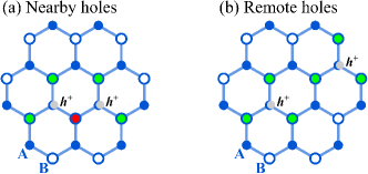
Figure S1: Configurations of two-hole states. (a) Two nearby holes that are connected by a common B site. (b) Two remote holes. The virtual tunneling induced attraction involves B sites, and we need to compare the energy difference between (a) and (b). The white circles correspond to the on-site energy correction $E_{v}^{(0)}$ (without any nearest-neighbor hole), the green circles correspond to the on-site energy correction $E_{v}^{(1)}$ (with one nearest-neighbor hole), the red circles correspond to the on-site energy correction $E_{v}^{(2)}$ (with two nearest-neighbor holes).

IV Microscopic interlayer tunneling

In the BBG-WSe₂ experiment, there is a relative angle $\theta$ between WSe₂ and BBG. In addition, the lattice constant of WSe₂ is $d=0.331$nm which is larger than the lattice constant of graphene, $a=0.246$nm. These two factors are crucial for the microscopic interlayer tunneling, which are discussed in the section.

First of all, the interlayer tunneling preserves the crystal momentum because we assume that the tunneling between two positions depends only on their relative displacement. In our case, the Brillouin zones of WSe₂ and BBG are in different sizes, and WSe₂ is rotated by an angle $\theta$. In Fig. S2, the Brillouin zones for both the WSe₂ and BBG are illustrated. Within the two-center approximation scheme, the spin-preserving tunneling between two layers (from the $\beta$th band with sublattice $\sigma^{\prime}$ to the $\alpha$ band with sublattice $\sigma$) can be described by Bistritzer and MacDonald (2010)

$$T_{\bm{\mathrm{k}},\bm{\mathrm{p}}}^{\alpha,\sigma;\beta,\sigma^{\prime}}\equiv T(\alpha,\sigma,\bm{\mathrm{k}};\beta,\sigma^{\prime},\bm{\mathrm{p}})= \frac{1}{\sqrt{\mathcal{A}_{0}\mathcal{A}_{1}}}\left(a^{(1)}_{\bm{\mathrm{k}},\alpha,\sigma}\right)^{*}\left(a^{(0)}_{\bm{\mathrm{p}},\beta,\sigma^{\prime}}\right)\!\sum_{\bm{\mathrm{Q}}^{(1)},\bm{\mathrm{Q}}^{(0)}}\tilde{t}_{\bm{\mathrm{k}}+\bm{\mathrm{Q}}^{(1)}}e^{i\bm{\mathrm{Q}}^{(1)}\cdot\bm{\mathrm{R}}^{(1)}_{\sigma}}e^{-i\bm{\mathrm{Q}}^{(0)}\cdot\bm{\mathrm{R}}^{(0)}_{\sigma^{\prime}}}\delta_{\bm{\mathrm{k}}+\bm{\mathrm{Q}}^{(1)},\bm{\mathrm{p}}+\bm{\mathrm{Q}}^{(0)}},$$ (S48)

where $\mathcal{A}_{0}$ ($\mathcal{A}_{1}$) is unit cell area of the WSe₂ (graphene), $\alpha$ and $\beta$ are the band indexes, $\bm{\mathrm{k}}$ and $\bm{\mathrm{p}}^{\prime}$ are the momentum relative to $\Gamma$ point, $\sigma$ and $\sigma^{\prime}$ are the sublattice indexes, $a^{(l)}_{\bm{\mathrm{k}},\alpha,\sigma}$ is the sublattice projection of a Bloch state $|\bm{\mathrm{k}},\alpha\rangle$ at layer $l$, $\bm{\mathrm{R}}^{(l)}_{\sigma}$ is the sublattice vector of $l$th layer, $\bm{\mathrm{Q}}^{(0)}$ and $\bm{\mathrm{Q}}^{(1)}$ represent the reciprocal lattice vectors in WSe₂ and BBG, respectively, and $\tilde{t}_{\bm{\mathrm{k}}}$ is the 2D Fourier transform of the interlayer tunneling amplitude with a finite range. $T(\alpha,\sigma,\bm{\mathrm{k}};\beta,\sigma^{\prime},\bm{\mathrm{p}})$ indicates the components of both bands and sublattices. In the above expression, we use index $0$ as the WSe₂ layer and index $1$ as the top graphene layer of BBG. We have ignored relative layer shift $\bm{\mathrm{d}}$ for simplicity. $\bm{\mathrm{Q}}^{(0)}=n_{0}\bm{\mathrm{G}}^{(0)}_{1}+m_{0}\bm{\mathrm{G}}^{(0)}_{2}$ and $\bm{\mathrm{Q}}^{(1)}=n_{1}\bm{\mathrm{G}}^{(1)}_{1}+m_{1}\bm{\mathrm{G}}^{(1)}_{2}$ for integer values of $n_{0}$, $m_{0}$, $n_{1}$, $m_{1}$, and $\bm{\mathrm{G}}^{(0)}_{1}$, $\bm{\mathrm{G}}^{(0)}_{2}$, $\bm{\mathrm{G}}^{(1)}_{1}$, $\bm{\mathrm{G}}^{(1)}_{2}$ are the primitive lattice vectors for the reciprocal lattices as illustrated in Fig. S2. $\bm{\mathrm{R}}^{(0)}_{A}=(0,0)$, $\bm{\mathrm{R}}^{(0)}_{B}=(0,d/\sqrt{3})$, $\bm{\mathrm{R}}^{(1)}_{A}=(0,0)$, and $\bm{\mathrm{R}}^{(1)}_{B}=(0,a/\sqrt{3})$.

Equation (S48) describes the microscopic interlayer tunneling between two layers. The contributions come from infinitely many crystal momenta, but the contributions from the large crystal momentum $\bm{\mathrm{k}}$ is suppressed by $\tilde{t}_{\bm{\mathrm{k}}}$, which can be modeled as a stretched exponentially decaying function in $\bm{\mathrm{k}}$ Bistritzer and MacDonald (2010) (will be discussed later). In addition, the contribution is small if the momentum $\bm{\mathrm{k}}$ is too far away from the valleys due to the structure of $a^{(l)}_{\bm{\mathrm{k}},\alpha,\sigma}$.

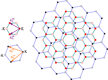
Figure S2: Brillouin zones of WSe₂ and BBG. The green (blue) lines indicate the reciprocal lattice of WSe₂ (BBG). The blue lattice is rotated by an angle $\theta=10^{\circ}$ in this illustration. $\bm{\mathrm{G}}^{(0)}_{1}=\left(-\frac{2\pi}{d},\frac{2\pi}{\sqrt{3}d}\right)$, $\bm{\mathrm{G}}^{(0)}_{2}=\left(-\frac{2\pi}{d},-\frac{2\pi}{\sqrt{3}d}\right)$, $\bm{\mathrm{G}}^{(1)}_{1}=\frac{2\pi}{a}\left(-\cos\theta-\frac{\sin\theta}{\sqrt{3}},\frac{\cos\theta}{\sqrt{3}}-\sin\theta\right)$, $\bm{\mathrm{G}}^{(1)}_{2}=\frac{2\pi}{a}\left(-\cos\theta+\frac{\sin\theta}{\sqrt{3}},-\frac{\cos\theta}{\sqrt{3}}-\sin\theta\right)$.

Our main purpose is to connect the microscopic calculations to the minimal model approach. We focus only on the tunneling between the $d_{x^{2}-y^{2}}\pm id_{xy}$ orbitals of WSe₂ and the top graphene layer of BBG. Since our theory is based on electrons tunneling from WSe₂ valence bands, only the 1st and 2nd bands in $\hat{h}_{\tau}^{(\text{WSe}_{2})}(\bm{\mathrm{k}})$ [given by Eq. (S33)] are considered. With respect to BBG, only the 2nd and 4th bands in $\hat{h}_{\tau}(\bm{\mathrm{k}})$ [given by Eq. (S5)] are considered because these two bands are relevant to the intervalley tunneling in our model. To simplify our calculations, we keep only $K$ and $-K$ momenta in BBG bands, and we consider a momentum cutoff $\bar{\Lambda}$ (relative to $\bar{K}$ or $-\bar{K}$) for WSe₂ bands. We define $\bm{\mathrm{K}}_{0}=\frac{4\pi}{3d}(1,0)$ and $\bm{\mathrm{K}}_{1}=\frac{4\pi}{3a}(\cos\theta,\sin\theta)$, where $a=0.246$nm (lattice constant of graphene) and $d=0.331$nm (lattice constant of WSe₂).

IV.1 ISOC and virtual-tunneling-induced attraction

In the main text, we discuss ideas of deriving ISOC and the virtual-hopping-induced attraction. The same procedures can be done with the microscopic interlayer tunneling. The main differences is that multiple momenta states in WSe₂ can contribute to the virtual processes instead of one. This is a consequence of the moiré structure of the BBG-WSe₂ such that crystal momentum conservation can allow for tunnelings from extended zones.

We can formally compute ISOC based on second order perturbation theory of the microscopic interlayer tunneling and derive that

$$\lambda_{I}=\sum_{\bm{\mathrm{q}},|\bm{\mathrm{q}}|<\bar{\Lambda}}\left[\begin{array}[]{c}\frac{\left|T(2,A,\bm{\mathrm{K}}_{1};2,B,\bm{\mathrm{K}}_{0}+\bm{\mathrm{q}})\right|^{2}}{-E_{2}^{(\text{WSe}_{2})}(\bm{\mathrm{q}})+2\Delta}-\frac{\left|T(2,A,\bm{\mathrm{K}}_{1};1,B,\bm{\mathrm{K}}_{0}+\bm{\mathrm{q}})\right|^{2}}{-E_{1}^{(\text{WSe}_{2})}(\bm{\mathrm{q}})+2\Delta}-\frac{\left|T(2,A,-\bm{\mathrm{K}}_{1};2,B,\bm{\mathrm{K}}_{0}+\bm{\mathrm{q}})\right|^{2}}{-E_{2}^{(\text{WSe}_{2})}(\bm{\mathrm{q}})+2\Delta}+\frac{\left|T(2,A,-\bm{\mathrm{K}}_{1};1,B,\bm{\mathrm{K}}_{0}+\bm{\mathrm{q}})\right|^{2}}{-E_{1}^{(\text{WSe}_{2})}(\bm{\mathrm{q}})+2\Delta}\end{array}\right],$$ (S50)

where we have incorporated the potential energy difference ($2\Delta$) between WSe₂ and the top graphene layer (assuming the same distance as the top and bottom graphene layers) and $\bar{\Lambda}$ is the cutoff for the momentum sum. $\bar{\Lambda}\leq\frac{2\pi}{3d}$ is required for consistently defining valleys. In this work, we use $\bar{\Lambda}=\frac{2\pi}{3d}=0.633$Å^-1. With the above expression and Eq. (S41), we identify that

$$\frac{\left|V^{A}_{+\uparrow}\right|^{2}}{W}= \sum_{\bm{\mathrm{q}},|\bm{\mathrm{q}}|<\bar{\Lambda}}\frac{\left|T(2,A,\bm{\mathrm{K}}_{1};2,B,\bm{\mathrm{K}}_{0}+\bm{\mathrm{q}})\right|^{2}}{-E_{2}^{(\text{WSe}_{2})}(\bm{\mathrm{q}})+2\Delta},$$ (S51a)

$$\frac{\left|V^{A}_{+\downarrow}\right|^{2}}{W+\delta}= \sum_{\bm{\mathrm{q}},|\bm{\mathrm{q}}|<\bar{\Lambda}}\frac{\left|T(2,A,\bm{\mathrm{K}}_{1};1,B,\bm{\mathrm{K}}_{0}+\bm{\mathrm{q}})\right|^{2}}{-E_{1}^{(\text{WSe}_{2})}(\bm{\mathrm{q}})+2\Delta},$$ (S51b)

$$\frac{\left|\bar{V}^{A}_{+\uparrow}\right|^{2}}{W}= \sum_{\bm{\mathrm{q}},|\bm{\mathrm{q}}|<\bar{\Lambda}}\frac{\left|T(2,A,-\bm{\mathrm{K}}_{1};2,B,\bm{\mathrm{K}}_{0}+\bm{\mathrm{q}})\right|^{2}}{-E_{2}^{(\text{WSe}_{2})}(\bm{\mathrm{q}})+2\Delta},$$ (S51c)

$$\frac{\left|\bar{V}^{A}_{+\downarrow}\right|^{2}}{W+\delta}= \sum_{\bm{\mathrm{q}},|\bm{\mathrm{q}}|<\bar{\Lambda}}\frac{\left|T(2,A,-\bm{\mathrm{K}}_{1};1,B,\bm{\mathrm{K}}_{0}+\bm{\mathrm{q}})\right|^{2}}{-E_{1}^{(\text{WSe}_{2})}(\bm{\mathrm{q}})+2\Delta}.$$ (S51d)

Similarly, we can compute the virtual-tunneling-induced attraction and derive that

$$\mathcal{U}_{\text{eff}}=2\sum_{\bm{\mathrm{q}},|\bm{\mathrm{q}}|<\bar{\Lambda}}\left[\begin{array}[]{c}\frac{\left|T(4,B,\bm{\mathrm{K}}_{1};2,B,\bm{\mathrm{K}}_{0}+\bm{\mathrm{q}})\right|^{2}}{-E_{2}^{(\text{WSe}_{2})}(\bm{\mathrm{q}})+2\Delta+E_{B}}+\frac{\left|T(4,B,-\bm{\mathrm{K}}_{1};2,B,\bm{\mathrm{K}}_{0}+\bm{\mathrm{q}})\right|^{2}}{-E_{2}^{(\text{WSe}_{2})}(\bm{\mathrm{q}})+2\Delta+E_{B}}+\frac{\left|T(4,B,\bm{\mathrm{K}}_{1};1,B,\bm{\mathrm{K}}_{0}+\bm{\mathrm{q}})\right|^{2}}{-E_{1}^{(\text{WSe}_{2})}(\bm{\mathrm{q}})+2\Delta+E_{B}}+\frac{\left|T(4,B,-\bm{\mathrm{K}}_{1};1,B,\bm{\mathrm{K}}_{0}+\bm{\mathrm{q}})\right|^{2}}{-E_{1}^{(\text{WSe}_{2})}(\bm{\mathrm{q}})+2\Delta+E_{B}}\\[11.38109pt] +\frac{\left|T(4,B,\bm{\mathrm{K}}_{1};2,B,\bm{\mathrm{K}}_{0}+\bm{\mathrm{q}})\right|^{2}}{-E_{2}^{(\text{WSe}_{2})}(\bm{\mathrm{q}})+2\Delta+E_{B}-2U_{1}}+\frac{\left|T(4,B,-\bm{\mathrm{K}}_{1};2,B,\bm{\mathrm{K}}_{0}+\bm{\mathrm{q}})\right|^{2}}{-E_{2}^{(\text{WSe}_{2})}(\bm{\mathrm{q}})+2\Delta+E_{B}-2U_{1}}+\frac{\left|T(4,B,\bm{\mathrm{K}}_{1};1,B,\bm{\mathrm{K}}_{0}+\bm{\mathrm{q}})\right|^{2}}{-E_{1}^{(\text{WSe}_{2})}(\bm{\mathrm{q}})+2\Delta+E_{B}-2U_{1}}+\frac{\left|T(4,B,-\bm{\mathrm{K}}_{1};1,B,\bm{\mathrm{K}}_{0}+\bm{\mathrm{q}})\right|^{2}}{-E_{1}^{(\text{WSe}_{2})}(\bm{\mathrm{q}})+2\Delta+E_{B}-2U_{1}}\\[11.38109pt] -2\frac{\left|T(4,B,\bm{\mathrm{K}}_{1};2,B,\bm{\mathrm{K}}_{0}+\bm{\mathrm{q}})\right|^{2}}{-E_{2}^{(\text{WSe}_{2})}(\bm{\mathrm{q}})+2\Delta+E_{B}-U_{1}}-2\frac{\left|T(4,B,-\bm{\mathrm{K}}_{1};2,B,\bm{\mathrm{K}}_{0}+\bm{\mathrm{q}})\right|^{2}}{-E_{2}^{(\text{WSe}_{2})}(\bm{\mathrm{q}})+2\Delta+E_{B}-U_{1}}-2\frac{\left|T(4,B,\bm{\mathrm{K}}_{1};1,B,\bm{\mathrm{K}}_{0}+\bm{\mathrm{q}})\right|^{2}}{-E_{1}^{(\text{WSe}_{2})}(\bm{\mathrm{q}})+2\Delta+E_{B}-U_{1}}-2\frac{\left|T(4,B,-\bm{\mathrm{K}}_{1};1,B,\bm{\mathrm{K}}_{0}+\bm{\mathrm{q}})\right|^{2}}{-E_{1}^{(\text{WSe}_{2})}(\bm{\mathrm{q}})+2\Delta+E_{B}-U_{1}}\end{array}\right].$$ (S55)

With the above expression and Eq (III.2), we identify that

$$\frac{\left|V^{B}_{+\uparrow}\right|^{2}}{W+E_{B}-xU_{1}}= \sum_{\bm{\mathrm{q}},|\bm{\mathrm{q}}|<\bar{\Lambda}}\frac{\left|T(4,B,\bm{\mathrm{K}}_{1};2,B,\bm{\mathrm{K}}_{0}+\bm{\mathrm{q}})\right|^{2}}{-E_{2}^{(\text{WSe}_{2})}(\bm{\mathrm{q}})+2\Delta+E_{B}-xU_{1}},$$ (S56a)

$$\frac{\left|V^{B}_{+\downarrow}\right|^{2}}{W+\delta+E_{B}-xU_{1}}= \sum_{\bm{\mathrm{q}},|\bm{\mathrm{q}}|<\bar{\Lambda}}\frac{\left|T(4,B,\bm{\mathrm{K}}_{1};1,B,\bm{\mathrm{K}}_{0}+\bm{\mathrm{q}})\right|^{2}}{-E_{1}^{(\text{WSe}_{2})}(\bm{\mathrm{q}})+2\Delta+E_{B}-xU_{1}},$$ (S56b)

$$\frac{\left|\bar{V}^{B}_{+\uparrow}\right|^{2}}{W+E_{B}-xU_{1}}= \sum_{\bm{\mathrm{q}},|\bm{\mathrm{q}}|<\bar{\Lambda}}\frac{\left|T(4,B,-\bm{\mathrm{K}}_{1};2,B,\bm{\mathrm{K}}_{0}+\bm{\mathrm{q}})\right|^{2}}{-E_{2}^{(\text{WSe}_{2})}(\bm{\mathrm{q}})+2\Delta+E_{B}-xU_{1}},$$ (S56c)

$$\frac{\left|\bar{V}^{B}_{+\downarrow}\right|^{2}}{W+\delta+E_{B}-xU_{1}}= \sum_{\bm{\mathrm{q}},|\bm{\mathrm{q}}|<\bar{\Lambda}}\frac{\left|T(4,B,-\bm{\mathrm{K}}_{1};1,B,\bm{\mathrm{K}}_{0}+\bm{\mathrm{q}})\right|^{2}}{-E_{1}^{(\text{WSe}_{2})}(\bm{\mathrm{q}})+2\Delta+E_{B}-xU_{1}},$$ (S56d)

where $x=0,1,2$.

IV.2 Evaluating interlayer tunneling

To compute $T(\alpha,\sigma,\bm{\mathrm{k}};\beta,\sigma^{\prime},\bm{\mathrm{p}})$, $a^{(l)}_{\bm{\mathrm{k}},\alpha,\sigma}$ and $\tilde{t}_{\bm{\mathrm{k}}}$ are needed. $a^{(l)}_{\bm{\mathrm{k}},\alpha,\sigma}$ corresponds to the wavefunctions of $\hat{h}_{\tau}^{(\text{WSe}_{2})}(\bm{\mathrm{k}})$ and $\hat{h}_{\tau}(\bm{\mathrm{k}})$, given by Eqs. (S33) and (S28). We find

$$a^{(0)}_{\bm{\mathrm{K}}_{0}+\bm{\mathrm{q}},1,B}=\frac{1}{\sqrt{1+\left[\frac{2v|\bm{\mathrm{q}}|}{\Omega+\lambda+\sqrt{4v^{2}\bm{\mathrm{q}}^{2}+(\Omega+\lambda)^{2}}}\right]^{2}}},\,\,a^{(0)}_{\bm{\mathrm{K}}_{0}+\bm{\mathrm{q}},2,B}=\frac{1}{\sqrt{1+\left[\frac{2v|\bm{\mathrm{q}}|}{\Omega-\lambda+\sqrt{4v^{2}\bm{\mathrm{q}}^{2}+(\Omega-\lambda)^{2}}}\right]^{2}}},\,\,a^{(1)}_{\pm\bm{\mathrm{K}}_{1},2,A}=1,\,\,a^{(1)}_{\pm\bm{\mathrm{K}}_{1},4,B}=\frac{1}{\sqrt{2}}.$$ (S57)

Based on the wavefunction amplitudes above, we conclude that $\left|T(2,A,\bm{\mathrm{K}}_{1};2,B,\bm{\mathrm{K}}_{0}+\bm{\mathrm{q}})\right|<\left|T(2,A,\bm{\mathrm{K}}_{1};1,B,\bm{\mathrm{K}}_{0}+\bm{\mathrm{q}})\right|$ and $\left|T(4,B,\bm{\mathrm{K}}_{1};2,B,\bm{\mathrm{K}}_{0}+\bm{\mathrm{q}})\right|<\left|T(4,B,\bm{\mathrm{K}}_{1};1,B,\bm{\mathrm{K}}_{0}+\bm{\mathrm{q}})\right|$, but the difference might be small. In addition, $\left|T(4,B,\bm{\mathrm{K}}_{1};1,B,\bm{\mathrm{K}}_{0}+\bm{\mathrm{q}})\right|=\frac{1}{\sqrt{2}}\left|T(2,A,\bm{\mathrm{K}}_{1};1,B,\bm{\mathrm{K}}_{0}+\bm{\mathrm{q}})\right|$ and $\left|T(4,B,\bm{\mathrm{K}}_{1};2,B,\bm{\mathrm{K}}_{0}+\bm{\mathrm{q}})\right|=\frac{1}{\sqrt{2}}\left|T(2,A,\bm{\mathrm{K}}_{1};2,B,\bm{\mathrm{K}}_{0}+\bm{\mathrm{q}})\right|$.

Regarding $\tilde{t}_{\bm{\mathrm{k}}}$, we follow Ref. Bistritzer and MacDonald (2010) and adopt a stretched exponential ansatz as follows:

$$|\tilde{t}_{\bm{\mathrm{k}}}|=t_{0}e^{-\chi(|\bm{\mathrm{k}}|z_{\perp})^{\gamma}},$$ (S58)

where $t_{0}$ is an overall constant, $\chi$ is an order 1 numerical constant, $\gamma$ is the exponent of stretched exponential, and $z_{\perp}$ is the distance between WSe₂ monolayer and the top graphene layer of BBG. We use $z_{\perp}=3.34$Å, the same as the distance between two graphene layers. $\chi$ and $\gamma$ control the decay of $\tilde{t}_{\bm{\mathrm{k}}}$ for a sufficiently large $\bm{\mathrm{k}}$, and we will discuss the results with a few representative values of $\chi$ and $\gamma$ in addition to the twist angle $\theta$. Since $\tilde{t}_{\bm{\mathrm{k}}}$ becomes small for a sufficiently large $\bm{\mathrm{k}}$, we can ignore contributions such that $\bm{\mathrm{k}}+\bm{\mathrm{Q}}^{(1)}>\Lambda$ in Eq. (S48), where we use $\Lambda=\frac{4\pi}{a}=5.11$Å^-1.

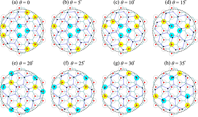
Figure S3: Kinematics of tunneling matrix elements with different angles. The green and the blue lines draw the Brillouin zone boundaries of WSe₂ and BBG, respectively. The gray circles with dashed lines indicate the cutoff $\bar{\Lambda}$ of the momentum relative to the $\bar{K}$ valleys (marked by red solid dots) of WSe₂. The big black circle with dashed lines indicates the cutoff $\Lambda$ of the total momentum (relative to $\Gamma$ point in the first Brillouin zone). The blue regions and yellow regions indicate the finite contributions of intravalley and intervalley tunnelings, respectively. The black solid (opened) dots denote the $K$ ($-K$) valleys of BBG.

In Fig. S3, the kinematics of momenta involved in tunneling is plotted for a few values of $\theta$. The big black dashed circle draws the region of $\bm{\mathrm{k}}+\bm{\mathrm{Q}}^{(1)}<\Lambda$ considered in the tunneling. We also use the small gray dashed circles to mark the momentum cutoff $\bar{\Lambda}$ for momentum relative to $\bar{K}$ valley. The blue circles indicate finite contributions of intravalley processes; the yellow circles indicate finite contributions of intervalley processes. Now, we are in the position to compute interlayer tunneling between WSe₂ and BBG.

IV.3 $T(\alpha,\sigma,k;\beta,\sigma^{\prime},p)$ at different angles

The interlayer tunneling matrix element crucially depends on the twist angle $\theta$. In Fig. S3, we plot crystal momenta involved in the interlayer tunneling with different $\theta$. We will list all the needed tunneling matrix elements for $0\leq\theta\leq 30^{\circ}$. In our model, angle $60^{\circ}-\theta$ is related to $\theta$, but the intravalley and intervalley contributions are interchanged. See the kinematics in Figs. S3(f) and S3(h) for an example.

IV.3.1 $\theta=0$

For $\theta=0$, there are three momenta contributing to the intravalley tunnelings and six momenta contributing to the intervalley tunnelings. Since the three intravalley tunnelings are related by the $\mathcal{C}_{3z}$ rotation, we only need to evaluate one of them. The six intervalley tunneling momenta are also related by symmetry operation, so only one of them needs to be evaluated. The spin-dependent interlayer tunneling terms are as follows:

$$\left|T(2,A,\bm{\mathrm{K}}_{1};2,B,\bm{\mathrm{K}}_{0}+\bm{\mathrm{q}})\right|^{2}\bigg{|}_{\bm{\mathrm{q}}=\bm{\mathrm{K}}_{1}-\bm{\mathrm{K}}_{0}}\approx \frac{t_{0}^{2}}{\mathcal{A}_{0}\mathcal{A}_{1}}\frac{e^{-2\chi(|\bm{\mathrm{K}}_{1}|z_{\perp})^{\gamma}}}{1+\left[\frac{2v|\bm{\mathrm{K}}_{1}-\bm{\mathrm{K}}_{0}|}{\Omega-\lambda+\sqrt{4v^{2}|\bm{\mathrm{K}}_{1}-\bm{\mathrm{K}}_{0}|^{2}+(\Omega-\lambda)^{2}}}\right]^{2}},$$ (S59a)

$$\left|T(2,A,\bm{\mathrm{K}}_{1};1,B,\bm{\mathrm{K}}_{0}+\bm{\mathrm{q}})\right|^{2}\bigg{|}_{\bm{\mathrm{q}}=\bm{\mathrm{K}}_{1}-\bm{\mathrm{K}}_{0}}\approx \frac{t_{0}^{2}}{\mathcal{A}_{0}\mathcal{A}_{1}}\frac{e^{-2\chi(|\bm{\mathrm{K}}_{1}|z_{\perp})^{\gamma}}}{1+\left[\frac{2v|\bm{\mathrm{K}}_{1}-\bm{\mathrm{K}}_{0}|}{\Omega+\lambda+\sqrt{4v^{2}|\bm{\mathrm{K}}_{1}-\bm{\mathrm{K}}_{0}|^{2}+(\Omega+\lambda)^{2}}}\right]^{2}},$$ (S59b)

$$\left|T(2,A,-\bm{\mathrm{K}}_{1};2,B,\bm{\mathrm{K}}_{0}+\bm{\mathrm{q}})\right|^{2}\bigg{|}_{\bm{\mathrm{q}}=-\bm{\mathrm{K}}_{1}-2\bm{\mathrm{G}}^{(1)}_{2}-[\bm{\mathrm{K}}_{0}+\bm{\mathrm{G}}^{(0)}_{1}-2\bm{\mathrm{G}}^{(0)}_{2}]}\approx \frac{t_{0}^{2}}{\mathcal{A}_{0}\mathcal{A}_{1}}\frac{e^{-2\chi\left(\mathcal{K}z_{\perp}\right)^{\gamma}}}{1+\left[\frac{2v\Delta k}{\Omega-\lambda+\sqrt{4v^{2}\Delta k^{2}+(\Omega-\lambda)^{2}}}\right]^{2}},$$ (S59c)

$$\left|T(2,A,-\bm{\mathrm{K}}_{1};1,B,\bm{\mathrm{K}}_{0}+\bm{\mathrm{q}})\right|^{2}\bigg{|}_{\bm{\mathrm{q}}=-\bm{\mathrm{K}}_{1}-2\bm{\mathrm{G}}^{(1)}_{2}-[\bm{\mathrm{K}}_{0}+\bm{\mathrm{G}}^{(0)}_{1}-2\bm{\mathrm{G}}^{(0)}_{2}]}\approx \frac{t_{0}^{2}}{\mathcal{A}_{0}\mathcal{A}_{1}}\frac{e^{-2\chi\left(\mathcal{K}z_{\perp}\right)^{\gamma}}}{1+\left[\frac{2v\Delta k}{\Omega+\lambda+\sqrt{4v^{2}\Delta k^{2}+(\Omega+\lambda)^{2}}}\right]^{2}},$$ (S59d)

where $|\bm{\mathrm{K}}_{1}-\bm{\mathrm{K}}_{0}|=0.437$Å^-1, $\Delta k=|-\bm{\mathrm{K}}_{1}-2\bm{\mathrm{G}}^{(1)}_{2}-\bm{\mathrm{K}}_{0}-\bm{\mathrm{G}}^{(0)}_{1}+2\bm{\mathrm{G}}^{(0)}_{2}|=0.416$Å^-1 and $\mathcal{K}=|-\bm{\mathrm{K}}_{1}-2\bm{\mathrm{G}}^{(1)}_{2}|=4.51$Å^-1.

IV.3.2 $\theta=5^{\circ}$

For $\theta=5^{\circ}$, there are only two distinct momenta. The spin-dependent interlayer tunneling terms are as follows:

$$\left|T(2,A,\bm{\mathrm{K}}_{1};2,B,\bm{\mathrm{K}}_{0}+\bm{\mathrm{q}})\right|^{2}\bigg{|}_{\bm{\mathrm{q}}=\bm{\mathrm{K}}_{1}-\bm{\mathrm{K}}_{0}}\approx \frac{t_{0}^{2}}{\mathcal{A}_{0}\mathcal{A}_{1}}\frac{e^{-2\chi(|\bm{\mathrm{K}}_{1}|z_{\perp})^{\gamma}}}{1+\left[\frac{2v|\bm{\mathrm{K}}_{1}-\bm{\mathrm{K}}_{0}|}{\Omega-\lambda+\sqrt{4v^{2}|\bm{\mathrm{K}}_{1}-\bm{\mathrm{K}}_{0}|^{2}+(\Omega-\lambda)^{2}}}\right]^{2}},$$ (S60a)

$$\left|T(2,A,\bm{\mathrm{K}}_{1};1,B,\bm{\mathrm{K}}_{0}+\bm{\mathrm{q}})\right|^{2}\bigg{|}_{\bm{\mathrm{q}}=\bm{\mathrm{K}}_{1}-\bm{\mathrm{K}}_{0}}\approx \frac{t_{0}^{2}}{\mathcal{A}_{0}\mathcal{A}_{1}}\frac{e^{-2\chi(|\bm{\mathrm{K}}_{1}|z_{\perp})^{\gamma}}}{1+\left[\frac{2v|\bm{\mathrm{K}}_{1}-\bm{\mathrm{K}}_{0}|}{\Omega+\lambda+\sqrt{4v^{2}|\bm{\mathrm{K}}_{1}-\bm{\mathrm{K}}_{0}|^{2}+(\Omega+\lambda)^{2}}}\right]^{2}},$$ (S60b)

$$\left|T(2,A,-\bm{\mathrm{K}}_{1};2,B,\bm{\mathrm{K}}_{0}+\bm{\mathrm{q}})\right|^{2}\bigg{|}_{\bm{\mathrm{q}}=-\bm{\mathrm{K}}_{1}-2\bm{\mathrm{G}}^{(1)}_{2}-[\bm{\mathrm{K}}_{0}+\bm{\mathrm{G}}^{(0)}_{1}-2\bm{\mathrm{G}}^{(0)}_{2}]}\approx \frac{t_{0}^{2}}{\mathcal{A}_{0}\mathcal{A}_{1}}\frac{e^{-2\chi\left(\mathcal{K}z_{\perp}\right)^{\gamma}}}{1+\left[\frac{2v\Delta k}{\Omega-\lambda+\sqrt{4v^{2}\Delta k^{2}+(\Omega-\lambda)^{2}}}\right]^{2}},$$ (S60c)

$$\left|T(2,A,-\bm{\mathrm{K}}_{1};1,B,\bm{\mathrm{K}}_{0}+\bm{\mathrm{q}})\right|^{2}\bigg{|}_{\bm{\mathrm{q}}=-\bm{\mathrm{K}}_{1}-2\bm{\mathrm{G}}^{(1)}_{2}-[\bm{\mathrm{K}}_{0}+\bm{\mathrm{G}}^{(0)}_{1}-2\bm{\mathrm{G}}^{(0)}_{2}]}\approx \frac{t_{0}^{2}}{\mathcal{A}_{0}\mathcal{A}_{1}}\frac{e^{-2\chi\left(\mathcal{K}z_{\perp}\right)^{\gamma}}}{1+\left[\frac{2v\Delta k}{\Omega+\lambda+\sqrt{4v^{2}\Delta k^{2}+(\Omega+\lambda)^{2}}}\right]^{2}},$$ (S60d)

where $|\bm{\mathrm{K}}_{1}-\bm{\mathrm{K}}_{0}|=0.456$Å^-1, $\Delta k=|-\bm{\mathrm{K}}_{1}-2\bm{\mathrm{G}}^{(1)}_{2}-\bm{\mathrm{K}}_{0}-\bm{\mathrm{G}}^{(0)}_{1}+2\bm{\mathrm{G}}^{(0)}_{2}|=0.06$Å^-1 and $\mathcal{K}=|-\bm{\mathrm{K}}_{1}-2\bm{\mathrm{G}}^{(1)}_{2}|=4.51$Å^-1. Since the intervalley processes have a very small $\Delta k$, the intervalley contribution can be large. This explains the weak nonmonotonicity in ISOC an effective attraction for $\gamma=1$ and $\chi=0.2$.

IV.3.3 $\theta=10^{\circ}$

For $\theta=10^{\circ}$, there are three distinct momenta. The spin-dependent interlayer tunneling terms are as follows:

$$\left|T(2,A,\bm{\mathrm{K}}_{1};2,B,\bm{\mathrm{K}}_{0}+\bm{\mathrm{q}})\right|^{2}\bigg{|}_{\bm{\mathrm{q}}=\bm{\mathrm{K}}_{1}-\bm{\mathrm{K}}_{0}}\approx \frac{t_{0}^{2}}{\mathcal{A}_{0}\mathcal{A}_{1}}\frac{e^{-2\chi(|\bm{\mathrm{K}}_{1}|z_{\perp})^{\gamma}}}{1+\left[\frac{2v|\bm{\mathrm{K}}_{1}-\bm{\mathrm{K}}_{0}|}{\Omega-\lambda+\sqrt{4v^{2}|\bm{\mathrm{K}}_{1}-\bm{\mathrm{K}}_{0}|^{2}+(\Omega-\lambda)^{2}}}\right]^{2}},$$ (S61a)

$$\left|T(2,A,\bm{\mathrm{K}}_{1};1,B,\bm{\mathrm{K}}_{0}+\bm{\mathrm{q}})\right|^{2}\bigg{|}_{\bm{\mathrm{q}}=\bm{\mathrm{K}}_{1}-\bm{\mathrm{K}}_{0}}\approx \frac{t_{0}^{2}}{\mathcal{A}_{0}\mathcal{A}_{1}}\frac{e^{-2\chi(|\bm{\mathrm{K}}_{1}|z_{\perp})^{\gamma}}}{1+\left[\frac{2v|\bm{\mathrm{K}}_{1}-\bm{\mathrm{K}}_{0}|}{\Omega+\lambda+\sqrt{4v^{2}|\bm{\mathrm{K}}_{1}-\bm{\mathrm{K}}_{0}|^{2}+(\Omega+\lambda)^{2}}}\right]^{2}},$$ (S61b)

$$\left|T(2,A,-\bm{\mathrm{K}}_{1};2,B,\bm{\mathrm{K}}_{0}+\bm{\mathrm{q}})\right|^{2}\bigg{|}_{\bm{\mathrm{q}}=-\bm{\mathrm{K}}_{1}-\bm{\mathrm{G}}^{(1)}_{1}-\bm{\mathrm{G}}^{(1)}_{2}-[\bm{\mathrm{K}}_{0}-\bm{\mathrm{G}}^{(0)}_{2}]}\approx \frac{t_{0}^{2}}{\mathcal{A}_{0}\mathcal{A}_{1}}\frac{e^{-2\chi\left(\mathcal{K}z_{\perp}\right)^{\gamma}}}{1+\left[\frac{2v\Delta k}{\Omega-\lambda+\sqrt{4v^{2}\Delta k^{2}+(\Omega-\lambda)^{2}}}\right]^{2}},$$ (S61c)

$$\left|T(2,A,-\bm{\mathrm{K}}_{1};1,B,\bm{\mathrm{K}}_{0}+\bm{\mathrm{q}})\right|^{2}\bigg{|}_{\bm{\mathrm{q}}=-\bm{\mathrm{K}}_{1}-\bm{\mathrm{G}}^{(1)}_{1}-\bm{\mathrm{G}}^{(1)}_{2}-[\bm{\mathrm{K}}_{0}-\bm{\mathrm{G}}^{(0)}_{2}]}\approx \frac{t_{0}^{2}}{\mathcal{A}_{0}\mathcal{A}_{1}}\frac{e^{-2\chi\left(\mathcal{K}z_{\perp}\right)^{\gamma}}}{1+\left[\frac{2v\Delta k}{\Omega+\lambda+\sqrt{4v^{2}\Delta k^{2}+(\Omega+\lambda)^{2}}}\right]^{2}},$$ (S61d)

$$\left|T(2,A,-\bm{\mathrm{K}}_{1};2,B,\bm{\mathrm{K}}_{0}+\bm{\mathrm{q}})\right|^{2}\bigg{|}_{\bm{\mathrm{q}}=-\bm{\mathrm{K}}_{1}-2\bm{\mathrm{G}}^{(1)}_{2}-[\bm{\mathrm{K}}_{0}+\bm{\mathrm{G}}^{(0)}_{1}-2\bm{\mathrm{G}}^{(0)}_{2}]}\approx \frac{t_{0}^{2}}{\mathcal{A}_{0}\mathcal{A}_{1}}\frac{e^{-2\chi\left(\mathcal{K}^{\prime}z_{\perp}\right)^{\gamma}}}{1+\left[\frac{2v\Delta k^{\prime}}{\Omega-\lambda+\sqrt{4v^{2}\Delta k^{\prime 2}+(\Omega-\lambda)^{2}}}\right]^{2}},$$ (S61e)

$$\left|T(2,A,-\bm{\mathrm{K}}_{1};1,B,\bm{\mathrm{K}}_{0}+\bm{\mathrm{q}})\right|^{2}\bigg{|}_{\bm{\mathrm{q}}=-\bm{\mathrm{K}}_{1}-2\bm{\mathrm{G}}^{(1)}_{2}-[\bm{\mathrm{K}}_{0}+\bm{\mathrm{G}}^{(0)}_{1}-2\bm{\mathrm{G}}^{(0)}_{2}]}\approx \frac{t_{0}^{2}}{\mathcal{A}_{0}\mathcal{A}_{1}}\frac{e^{-2\chi\left(\mathcal{K}^{\prime}z_{\perp}\right)^{\gamma}}}{1+\left[\frac{2v\Delta k^{\prime}}{\Omega+\lambda+\sqrt{4v^{2}\Delta k^{\prime 2}+(\Omega+\lambda)^{2}}}\right]^{2}},$$ (S61f)

where $|\bm{\mathrm{K}}_{1}-\bm{\mathrm{K}}_{0}|=0.507$Å^-1, $\Delta k=|-\bm{\mathrm{K}}_{1}-\bm{\mathrm{G}}^{(1)}_{1}-\bm{\mathrm{G}}^{(1)}_{2}-\bm{\mathrm{K}}_{0}+\bm{\mathrm{G}}^{(0)}_{2}|=0.539$Å^-1, $\mathcal{K}=|-\bm{\mathrm{K}}_{1}-\bm{\mathrm{G}}^{(1)}_{1}-\bm{\mathrm{G}}^{(1)}_{2}|=3.41$Å^-1, $\Delta k^{\prime}=|-\bm{\mathrm{K}}_{1}-2\bm{\mathrm{G}}^{(1)}_{2}-\bm{\mathrm{K}}_{0}-\bm{\mathrm{G}}^{(0)}_{1}+2\bm{\mathrm{G}}^{(0)}_{2}|=0.383$Å^-1, and $\mathcal{K}^{\prime}=|-\bm{\mathrm{K}}_{1}-2\bm{\mathrm{G}}^{(1)}_{2}|=4.51$Å^-1.

IV.3.4 $\theta=15^{\circ}$

For $\theta=15^{\circ}$, there are two distinct momenta. The spin-dependent interlayer tunneling terms are as follows:

$$\left|T(2,A,\bm{\mathrm{K}}_{1};2,B,\bm{\mathrm{K}}_{0}+\bm{\mathrm{q}})\right|^{2}\bigg{|}_{\bm{\mathrm{q}}=\bm{\mathrm{K}}_{1}-\bm{\mathrm{K}}_{0}}\approx \frac{t_{0}^{2}}{\mathcal{A}_{0}\mathcal{A}_{1}}\frac{e^{-2\chi(|\bm{\mathrm{K}}_{1}|z_{\perp})^{\gamma}}}{1+\left[\frac{2v|\bm{\mathrm{K}}_{1}-\bm{\mathrm{K}}_{0}|}{\Omega-\lambda+\sqrt{4v^{2}|\bm{\mathrm{K}}_{1}-\bm{\mathrm{K}}_{0}|^{2}+(\Omega-\lambda)^{2}}}\right]^{2}},$$ (S62a)

$$\left|T(2,A,\bm{\mathrm{K}}_{1};1,B,\bm{\mathrm{K}}_{0}+\bm{\mathrm{q}})\right|^{2}\bigg{|}_{\bm{\mathrm{q}}=\bm{\mathrm{K}}_{1}-\bm{\mathrm{K}}_{0}}\approx \frac{t_{0}^{2}}{\mathcal{A}_{0}\mathcal{A}_{1}}\frac{e^{-2\chi(|\bm{\mathrm{K}}_{1}|z_{\perp})^{\gamma}}}{1+\left[\frac{2v|\bm{\mathrm{K}}_{1}-\bm{\mathrm{K}}_{0}|}{\Omega+\lambda+\sqrt{4v^{2}|\bm{\mathrm{K}}_{1}-\bm{\mathrm{K}}_{0}|^{2}+(\Omega+\lambda)^{2}}}\right]^{2}},$$ (S62b)

$$\left|T(2,A,-\bm{\mathrm{K}}_{1};2,B,\bm{\mathrm{K}}_{0}+\bm{\mathrm{q}})\right|^{2}\bigg{|}_{\bm{\mathrm{q}}=-\bm{\mathrm{K}}_{1}-\bm{\mathrm{G}}^{(1)}_{1}-\bm{\mathrm{G}}^{(1)}_{2}-[\bm{\mathrm{K}}_{0}-\bm{\mathrm{G}}^{(0)}_{2}]}\approx \frac{t_{0}^{2}}{\mathcal{A}_{0}\mathcal{A}_{1}}\frac{e^{-2\chi\left(\mathcal{K}z_{\perp}\right)^{\gamma}}}{1+\left[\frac{2v\Delta k}{\Omega-\lambda+\sqrt{4v^{2}\Delta k^{2}+(\Omega-\lambda)^{2}}}\right]^{2}},$$ (S62c)

$$\left|T(2,A,-\bm{\mathrm{K}}_{1};1,B,\bm{\mathrm{K}}_{0}+\bm{\mathrm{q}})\right|^{2}\bigg{|}_{\bm{\mathrm{q}}=-\bm{\mathrm{K}}_{1}-\bm{\mathrm{G}}^{(1)}_{1}-\bm{\mathrm{G}}^{(1)}_{2}-[\bm{\mathrm{K}}_{0}-\bm{\mathrm{G}}^{(0)}_{2}]}\approx \frac{t_{0}^{2}}{\mathcal{A}_{0}\mathcal{A}_{1}}\frac{e^{-2\chi\left(\mathcal{K}z_{\perp}\right)^{\gamma}}}{1+\left[\frac{2v\Delta k}{\Omega+\lambda+\sqrt{4v^{2}\Delta k^{2}+(\Omega+\lambda)^{2}}}\right]^{2}},$$ (S62d)

where $|\bm{\mathrm{K}}_{1}-\bm{\mathrm{K}}_{0}|=0.581$Å^-1, $\Delta k=|-\bm{\mathrm{K}}_{1}-\bm{\mathrm{G}}^{(1)}_{1}-\bm{\mathrm{G}}^{(1)}_{2}-\bm{\mathrm{K}}_{0}+\bm{\mathrm{G}}^{(0)}_{2}|=0.249$Å^-1, and $\mathcal{K}=|-\bm{\mathrm{K}}_{1}-\bm{\mathrm{G}}^{(1)}_{1}-\bm{\mathrm{G}}^{(1)}_{2}|=3.41$Å^-1.

IV.3.5 $\theta=20^{\circ}$

For $\theta=20^{\circ}$, there are three distinct momenta. The spin-dependent interlayer tunneling terms are as follows:

$$\left|T(2,A,-\bm{\mathrm{K}}_{1};2,B,\bm{\mathrm{K}}_{0}+\bm{\mathrm{q}})\right|^{2}\bigg{|}_{\bm{\mathrm{q}}=-\bm{\mathrm{K}}_{1}-\bm{\mathrm{G}}^{(1)}_{1}-\bm{\mathrm{G}}^{(1)}_{2}-[\bm{\mathrm{K}}_{0}-\bm{\mathrm{G}}^{(0)}_{2}]}\approx \frac{t_{0}^{2}}{\mathcal{A}_{0}\mathcal{A}_{1}}\frac{e^{-2\chi\left(\mathcal{K}z_{\perp}\right)^{\gamma}}}{1+\left[\frac{2v\Delta k}{\Omega-\lambda+\sqrt{4v^{2}\Delta k^{2}+(\Omega-\lambda)^{2}}}\right]^{2}},$$ (S63a)

$$\left|T(2,A,-\bm{\mathrm{K}}_{1};1,B,\bm{\mathrm{K}}_{0}+\bm{\mathrm{q}})\right|^{2}\bigg{|}_{\bm{\mathrm{q}}=-\bm{\mathrm{K}}_{1}-\bm{\mathrm{G}}^{(1)}_{1}-\bm{\mathrm{G}}^{(1)}_{2}-[\bm{\mathrm{K}}_{0}-\bm{\mathrm{G}}^{(0)}_{2}]}\approx \frac{t_{0}^{2}}{\mathcal{A}_{0}\mathcal{A}_{1}}\frac{e^{-2\chi\left(\mathcal{K}z_{\perp}\right)^{\gamma}}}{1+\left[\frac{2v\Delta k}{\Omega+\lambda+\sqrt{4v^{2}\Delta k^{2}+(\Omega+\lambda)^{2}}}\right]^{2}},$$ (S63b)

$$\left|T(2,A,\bm{\mathrm{K}}_{1};2,B,\bm{\mathrm{K}}_{0}+\bm{\mathrm{q}})\right|^{2}\bigg{|}_{\bm{\mathrm{q}}=\bm{\mathrm{K}}_{1}-\bm{\mathrm{G}}^{(1)}_{1}-[\bm{\mathrm{K}}_{0}-\bm{\mathrm{G}}^{(0)}_{1}-\bm{\mathrm{G}}^{(0)}_{2}]}\approx \frac{t_{0}^{2}}{\mathcal{A}_{0}\mathcal{A}_{1}}\frac{e^{-2\chi\left(\mathcal{K}^{\prime}z_{\perp}\right)^{\gamma}}}{1+\left[\frac{2v\Delta k^{\prime}}{\Omega-\lambda+\sqrt{4v^{2}\Delta k^{\prime 2}+(\Omega-\lambda)^{2}}}\right]^{2}},$$ (S63c)

$$\left|T(2,A,\bm{\mathrm{K}}_{1};2,B,\bm{\mathrm{K}}_{0}+\bm{\mathrm{q}})\right|^{2}\bigg{|}_{\bm{\mathrm{q}}=\bm{\mathrm{K}}_{1}-\bm{\mathrm{G}}^{(1)}_{1}-[\bm{\mathrm{K}}_{0}-\bm{\mathrm{G}}^{(0)}_{1}-\bm{\mathrm{G}}^{(0)}_{2}]}\approx \frac{t_{0}^{2}}{\mathcal{A}_{0}\mathcal{A}_{1}}\frac{e^{-2\chi\left(\mathcal{K}^{\prime}z_{\perp}\right)^{\gamma}}}{1+\left[\frac{2v\Delta k^{\prime}}{\Omega+\lambda+\sqrt{4v^{2}\Delta k^{\prime 2}+(\Omega+\lambda)^{2}}}\right]^{2}},$$ (S63d)

$$\left|T(2,A,\bm{\mathrm{K}}_{1};2,B,\bm{\mathrm{K}}_{0}+\bm{\mathrm{q}})\right|^{2}\bigg{|}_{\bm{\mathrm{q}}=\bm{\mathrm{K}}_{1}-\bm{\mathrm{G}}^{(1)}_{2}-[\bm{\mathrm{K}}_{0}+\bm{\mathrm{G}}^{(0)}_{1}-2\bm{\mathrm{G}}^{(0)}_{2}]}\approx \frac{t_{0}^{2}}{\mathcal{A}_{0}\mathcal{A}_{1}}\frac{e^{-2\chi\left(\mathcal{K}^{\prime\prime}z_{\perp}\right)^{\gamma}}}{1+\left[\frac{2v\Delta k^{\prime\prime}}{\Omega-\lambda+\sqrt{4v^{2}\Delta k^{\prime\prime 2}+(\Omega-\lambda)^{2}}}\right]^{2}},$$ (S63e)

$$\left|T(2,A,\bm{\mathrm{K}}_{1};2,B,\bm{\mathrm{K}}_{0}+\bm{\mathrm{q}})\right|^{2}\bigg{|}_{\bm{\mathrm{q}}=\bm{\mathrm{K}}_{1}-\bm{\mathrm{G}}^{(1)}_{2}-[\bm{\mathrm{K}}_{0}+\bm{\mathrm{G}}^{(0)}_{1}-2\bm{\mathrm{G}}^{(0)}_{2}]}\approx \frac{t_{0}^{2}}{\mathcal{A}_{0}\mathcal{A}_{1}}\frac{e^{-2\chi\left(\mathcal{K}^{\prime\prime}z_{\perp}\right)^{\gamma}}}{1+\left[\frac{2v\Delta k^{\prime\prime}}{\Omega+\lambda+\sqrt{4v^{2}\Delta k^{\prime\prime 2}+(\Omega+\lambda)^{2}}}\right]^{2}},$$ (S63f)

where $\Delta k=|-\bm{\mathrm{K}}_{1}-\bm{\mathrm{G}}^{(1)}_{1}-\bm{\mathrm{G}}^{(1)}_{2}-\bm{\mathrm{K}}_{0}+\bm{\mathrm{G}}^{(0)}_{2}|=0.0778$Å^-1, $\mathcal{K}=|-\bm{\mathrm{K}}_{1}-\bm{\mathrm{G}}^{(1)}_{1}-\bm{\mathrm{G}}^{(1)}_{2}|=3.41$Å^-1, $\Delta k^{\prime}=|\bm{\mathrm{K}}_{1}-\bm{\mathrm{G}}^{(1)}_{1}-\bm{\mathrm{K}}_{0}+\bm{\mathrm{G}}^{(0)}_{1}+\bm{\mathrm{G}}^{(0)}_{2}|=0.562$Å^-1, $\mathcal{K}^{\prime}=|\bm{\mathrm{K}}_{1}-\bm{\mathrm{G}}^{(1)}_{1}|=4.51$Å^-1, $\Delta k^{\prime\prime}=|\bm{\mathrm{K}}_{1}-\bm{\mathrm{G}}^{(1)}_{2}-\bm{\mathrm{K}}_{0}-\bm{\mathrm{G}}^{(0)}_{1}+2\bm{\mathrm{G}}^{(0)}_{2}|=0.556$Å^-1, $\mathcal{K}^{\prime\prime}=|\bm{\mathrm{K}}_{1}-\bm{\mathrm{G}}^{(1)}_{2}|=4.51$Å^-1. At $\theta=20^{\circ}$, the intervalley processes have smaller crystal momentum than the intravalley processes. In addition, $\Delta k$ for the intervalley tunneling is quite small. This is why we find $\lambda_{I}<0$ at $\theta=20^{\circ}$. Another important point is that the tunneling crystal momentum is no longer at the first Brillouin zone corner (i.e., $K$ or $-K$). This explains the small effective attraction for $\theta\geq 20^{\circ}$

IV.3.6 $\theta=25^{\circ}$

For $\theta=25^{\circ}$, there are two distinct momenta. The spin-dependent interlayer tunneling terms are as follows:

$$\left|T(2,A,-\bm{\mathrm{K}}_{1};2,B,\bm{\mathrm{K}}_{0}+\bm{\mathrm{q}})\right|^{2}\bigg{|}_{\bm{\mathrm{q}}=-\bm{\mathrm{K}}_{1}-\bm{\mathrm{G}}^{(1)}_{1}-\bm{\mathrm{G}}^{(1)}_{2}-[\bm{\mathrm{K}}_{0}-\bm{\mathrm{G}}^{(0)}_{2}]}\approx \frac{t_{0}^{2}}{\mathcal{A}_{0}\mathcal{A}_{1}}\frac{e^{-2\chi\left(\mathcal{K}z_{\perp}\right)^{\gamma}}}{1+\left[\frac{2v\Delta k}{\Omega-\lambda+\sqrt{4v^{2}\Delta k^{2}+(\Omega-\lambda)^{2}}}\right]^{2}},$$ (S64a)

$$\left|T(2,A,-\bm{\mathrm{K}}_{1};1,B,\bm{\mathrm{K}}_{0}+\bm{\mathrm{q}})\right|^{2}\bigg{|}_{\bm{\mathrm{q}}=-\bm{\mathrm{K}}_{1}-\bm{\mathrm{G}}^{(1)}_{1}-\bm{\mathrm{G}}^{(1)}_{2}-[\bm{\mathrm{K}}_{0}-\bm{\mathrm{G}}^{(0)}_{2}]}\approx \frac{t_{0}^{2}}{\mathcal{A}_{0}\mathcal{A}_{1}}\frac{e^{-2\chi\left(\mathcal{K}z_{\perp}\right)^{\gamma}}}{1+\left[\frac{2v\Delta k}{\Omega+\lambda+\sqrt{4v^{2}\Delta k^{2}+(\Omega+\lambda)^{2}}}\right]^{2}},$$ (S64b)

$$\left|T(2,A,\bm{\mathrm{K}}_{1};2,B,\bm{\mathrm{K}}_{0}+\bm{\mathrm{q}})\right|^{2}\bigg{|}_{\bm{\mathrm{q}}=\bm{\mathrm{K}}_{1}-\bm{\mathrm{G}}^{(1)}_{2}-[\bm{\mathrm{K}}_{0}+\bm{\mathrm{G}}^{(0)}_{1}-2\bm{\mathrm{G}}^{(0)}_{2}]}\approx \frac{t_{0}^{2}}{\mathcal{A}_{0}\mathcal{A}_{1}}\frac{e^{-2\chi\left(\mathcal{K}^{\prime\prime}z_{\perp}\right)^{\gamma}}}{1+\left[\frac{2v\Delta k^{\prime\prime}}{\Omega-\lambda+\sqrt{4v^{2}\Delta k^{\prime\prime 2}+(\Omega-\lambda)^{2}}}\right]^{2}},$$ (S64c)

$$\left|T(2,A,\bm{\mathrm{K}}_{1};2,B,\bm{\mathrm{K}}_{0}+\bm{\mathrm{q}})\right|^{2}\bigg{|}_{\bm{\mathrm{q}}=\bm{\mathrm{K}}_{1}-\bm{\mathrm{G}}^{(1)}_{2}-[\bm{\mathrm{K}}_{0}+\bm{\mathrm{G}}^{(0)}_{1}-2\bm{\mathrm{G}}^{(0)}_{2}]}\approx \frac{t_{0}^{2}}{\mathcal{A}_{0}\mathcal{A}_{1}}\frac{e^{-2\chi\left(\mathcal{K}^{\prime\prime}z_{\perp}\right)^{\gamma}}}{1+\left[\frac{2v\Delta k^{\prime\prime}}{\Omega+\lambda+\sqrt{4v^{2}\Delta k^{\prime\prime 2}+(\Omega+\lambda)^{2}}}\right]^{2}},$$ (S64d)

where $\Delta k=|-\bm{\mathrm{K}}_{1}-\bm{\mathrm{G}}^{(1)}_{1}-\bm{\mathrm{G}}^{(1)}_{2}-\bm{\mathrm{K}}_{0}+\bm{\mathrm{G}}^{(0)}_{2}=0.352|$Å^-1, $\mathcal{K}=|-\bm{\mathrm{K}}_{1}-\bm{\mathrm{G}}^{(1)}_{1}-\bm{\mathrm{G}}^{(1)}_{2}|=3.41$Å^-1, $\Delta k^{\prime\prime}=|\bm{\mathrm{K}}_{1}-\bm{\mathrm{G}}^{(1)}_{2}-\bm{\mathrm{K}}_{0}-\bm{\mathrm{G}}^{(0)}_{1}+2\bm{\mathrm{G}}^{(0)}_{2}|=0.168$Å^-1, $\mathcal{K}^{\prime\prime}=|\bm{\mathrm{K}}_{1}-\bm{\mathrm{G}}^{(1)}_{2}|=4.51$Å^-1. Similar to $\theta=20^{\circ}$, the intervalley contributions are stronger than intravalley contributions, and $\lambda_{I}<0$ (albeit vanishingly small in some cases).

IV.3.7 $\theta=30^{\circ}$

For $\theta=30^{\circ}$, there is actually only one distinct momentum, but we check both intravalley and intervalley processes. The spin-dependent interlayer tunneling terms are as follows:

$$\left|T(2,A,-\bm{\mathrm{K}}_{1};2,B,\bm{\mathrm{K}}_{0}+\bm{\mathrm{q}})\right|^{2}\bigg{|}_{\bm{\mathrm{q}}=-\bm{\mathrm{K}}_{1}-2\bm{\mathrm{G}}^{(1)}_{2}-[\bm{\mathrm{K}}_{0}+2\bm{\mathrm{G}}^{(0)}_{1}-2\bm{\mathrm{G}}^{(0)}_{2}]}\approx \frac{t_{0}^{2}}{\mathcal{A}_{0}\mathcal{A}_{1}}\frac{e^{-2\chi\left(\mathcal{K}z_{\perp}\right)^{\gamma}}}{1+\left[\frac{2v\Delta k}{\Omega-\lambda+\sqrt{4v^{2}\Delta k^{2}+(\Omega-\lambda)^{2}}}\right]^{2}},$$ (S65a)

$$\left|T(2,A,-\bm{\mathrm{K}}_{1};1,B,\bm{\mathrm{K}}_{0}+\bm{\mathrm{q}})\right|^{2}\bigg{|}_{\bm{\mathrm{q}}=-\bm{\mathrm{K}}_{1}-2\bm{\mathrm{G}}^{(1)}_{2}-[\bm{\mathrm{K}}_{0}+2\bm{\mathrm{G}}^{(0)}_{1}-2\bm{\mathrm{G}}^{(0)}_{2}]}\approx \frac{t_{0}^{2}}{\mathcal{A}_{0}\mathcal{A}_{1}}\frac{e^{-2\chi\left(\mathcal{K}z_{\perp}\right)^{\gamma}}}{1+\left[\frac{2v\Delta k}{\Omega+\lambda+\sqrt{4v^{2}\Delta k^{2}+(\Omega+\lambda)^{2}}}\right]^{2}},$$ (S65b)

$$\left|T(2,A,\bm{\mathrm{K}}_{1};2,B,\bm{\mathrm{K}}_{0}+\bm{\mathrm{q}})\right|^{2}\bigg{|}_{\bm{\mathrm{q}}=\bm{\mathrm{K}}_{1}-\bm{\mathrm{G}}^{(1)}_{2}-[\bm{\mathrm{K}}_{0}+\bm{\mathrm{G}}^{(0)}_{1}-2\bm{\mathrm{G}}^{(0)}_{2}]}\approx \frac{t_{0}^{2}}{\mathcal{A}_{0}\mathcal{A}_{1}}\frac{e^{-2\chi\left(\mathcal{K}^{\prime\prime}z_{\perp}\right)^{\gamma}}}{1+\left[\frac{2v\Delta k^{\prime\prime}}{\Omega-\lambda+\sqrt{4v^{2}\Delta k^{\prime\prime 2}+(\Omega-\lambda)^{2}}}\right]^{2}},$$ (S65c)

$$\left|T(2,A,\bm{\mathrm{K}}_{1};2,B,\bm{\mathrm{K}}_{0}+\bm{\mathrm{q}})\right|^{2}\bigg{|}_{\bm{\mathrm{q}}=\bm{\mathrm{K}}_{1}-\bm{\mathrm{G}}^{(1)}_{2}-[\bm{\mathrm{K}}_{0}+\bm{\mathrm{G}}^{(0)}_{1}-2\bm{\mathrm{G}}^{(0)}_{2}]}\approx \frac{t_{0}^{2}}{\mathcal{A}_{0}\mathcal{A}_{1}}\frac{e^{-2\chi\left(\mathcal{K}^{\prime\prime}z_{\perp}\right)^{\gamma}}}{1+\left[\frac{2v\Delta k^{\prime\prime}}{\Omega+\lambda+\sqrt{4v^{2}\Delta k^{\prime\prime 2}+(\Omega+\lambda)^{2}}}\right]^{2}},$$ (S65d)

where $\Delta k=|\bm{\mathrm{q}}=-\bm{\mathrm{K}}_{1}-2\bm{\mathrm{G}}^{(1)}_{2}-\bm{\mathrm{K}}_{0}-2\bm{\mathrm{G}}^{(0)}_{1}+2\bm{\mathrm{G}}^{(0)}_{2}|=0.245$Å^-1, $\mathcal{K}=|-\bm{\mathrm{K}}_{1}-2\bm{\mathrm{G}}^{(1)}_{2}|=4.51$Å^-1, $\Delta k^{\prime\prime}=|\bm{\mathrm{K}}_{1}-\bm{\mathrm{G}}^{(1)}_{2}-\bm{\mathrm{K}}_{0}-\bm{\mathrm{G}}^{(0)}_{1}+2\bm{\mathrm{G}}^{(0)}_{2}|=0.245$Å^-1, and $\mathcal{K}^{\prime\prime}=|\bm{\mathrm{K}}_{1}-\bm{\mathrm{G}}^{(1)}_{2}|=4.51$Å^-1. $\lambda_{I}=0$ at $\theta=30^{\circ}$.

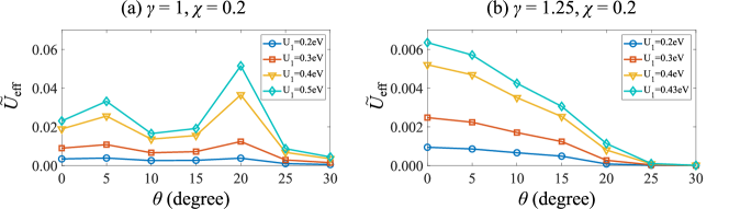
Figure S4: Effective attraction for different values of $U_{1}$. We plot the dimensionless spin-orbit coupling $\tilde{U}_{\text{eff}}=\mathcal{U}_{\text{eff}}\mathcal{A}_{0}\mathcal{A}_{1}\text{eV}/t_{0}^{2}$ as a function of $\theta$ with different values of $U_{1}$. We use $\gamma=1.25$ and $\chi=0.2$ in all the curves.

IV.4 Effective attraction versus $U_{1}$

Here, we discuss $U_{1}$ (short-range Coulomb interaction) dependence in the effective attraction strength $\mathcal{U}_{\text{eff}}$. In Fig. S4, we plot $\tilde{U}_{\text{eff}}=\mathcal{U}_{\text{eff}}\mathcal{A}_{0}\mathcal{A}_{1}\text{eV}/t_{0}^{2}$ (the dimensionless attraction) as a function of $\theta$ with (a) $\gamma=1$, $\chi=0.2$ and (b) $\gamma=1.25$, $\chi=0.2$ , and different values of $U_{1}$ ranging from 0.2eV to 0.43eV. ($U_{1}\leq E_{B}$ in our theory, where $E_{B}\approx 0.43$eV.) The qualitative trends are very similar because the values of $U_{1}$ do not generate extremely small denominators in second order perturbation theory. However, the results show quantitative dependence in $U_{1}$, and a larger $U_{1}$ generally enhances $\tilde{U}_{\text{eff}}$.

References

• Zhou et al. (2022) H. Zhou, L. Holleis, Y. Saito, L. Cohen, W. Huynh, C. L. Patterson, F. Yang, T. Taniguchi, K. Watanabe, and A. F. Young, Science 375, 774 (2022).
• Zhou et al. (2021a) H. Zhou, T. Xie, T. Taniguchi, K. Watanabe, and A. F. Young, Nature 598, 434 (2021a).
• Cao et al. (2018) Y. Cao, V. Fatemi, S. Fang, K. Watanabe, T. Taniguchi, E. Kaxiras, and P. Jarillo-Herrero, Nature 556, 43 (2018), URL http://dx.doi.org/10.1038/nature26160.
• Yankowitz et al. (2019) M. Yankowitz, S. Chen, H. Polshyn, Y. Zhang, K. Watanabe, T. Taniguchi, D. Graf, A. F. Young, and C. R. Dean, Science 363, 1059 (2019).
• Lu et al. (2019) X. Lu, P. Stepanov, W. Yang, M. Xie, M. A. Aamir, I. Das, C. Urgell, K. Watanabe, T. Taniguchi, G. Zhang, et al., Nature 574, 653 (2019).
• Hao et al. (2021) Z. Hao, A. Zimmerman, P. Ledwith, E. Khalaf, D. H. Najafabadi, K. Watanabe, T. Taniguchi, A. Vishwanath, and P. Kim, Science 371, 1133 (2021).
• Park et al. (2021a) J. M. Park, Y. Cao, K. Watanabe, T. Taniguchi, and P. Jarillo-Herrero, Nature 590, 249 (2021a).
• Cao et al. (2021) Y. Cao, J. M. Park, K. Watanabe, T. Taniguchi, and P. Jarillo-Herrero, Nature 595, 526 (2021).
• Liu et al. (2021) X. Liu, K. Watanabe, T. Taniguchi, and J. Li, arXiv preprint arXiv:2108.03338 (2021).
• Zhang et al. (2021) Y. Zhang, R. Polski, C. Lewandowski, A. Thomson, Y. Peng, Y. Choi, H. Kim, K. Watanabe, T. Taniguchi, J. Alicea, et al., arXiv preprint arXiv:2112.09270 (2021).
• Park et al. (2021b) J. M. Park, Y. Cao, L. Xia, S. Sun, K. Watanabe, T. Taniguchi, and P. Jarillo-Herrero, arXiv preprint arXiv:2112.10760 (2021b).
• Burg et al. (2022) G. W. Burg, E. Khalaf, Y. Wang, K. Watanabe, T. Taniguchi, and E. Tutuc, arXiv preprint arXiv:2201.01637 (2022).
• Siriviboon et al. (2021) P. Siriviboon, J. Lin, X. Liu, H. Scammell, S. Liu, D. Rhodes, K. Watanabe, T. Taniguchi, J. Hone, M. Scheurer, et al., arXiv preprint arXiv:2112.07127 (2021).
• Zhang et al. (2022) Y. Zhang, R. Polski, A. Thomson, É. Lantagne-Hurtubise, C. Lewandowski, H. Zhou, K. Watanabe, T. Taniguchi, J. Alicea, and S. Nadj-Perge, arXiv preprint arXiv:2205.05087 (2022).
• Zhou et al. (2021b) H. Zhou, T. Xie, A. Ghazaryan, T. Holder, J. R. Ehrets, E. M. Spanton, T. Taniguchi, K. Watanabe, E. Berg, M. Serbyn, et al., Nature 598, 429 (2021b).
• Chou et al. (2021a) Y.-Z. Chou, F. Wu, J. D. Sau, and S. Das Sarma, Phys. Rev. Lett. 127, 187001 (2021a), URL https://link.aps.org/doi/10.1103/PhysRevLett.127.187001.
• Chou et al. (2022a) Y.-Z. Chou, F. Wu, J. D. Sau, and S. Das Sarma, Phys. Rev. B 105, L100503 (2022a), URL https://link.aps.org/doi/10.1103/PhysRevB.105.L100503.
• Chou et al. (2022b) Y.-Z. Chou, F. Wu, J. D. Sau, and S. Das Sarma, arXiv preprint arXiv:2204.09811 (2022b).
• Chatterjee et al. (2021) S. Chatterjee, T. Wang, E. Berg, and M. P. Zaletel, arXiv preprint arXiv:2109.00002 (2021).
• Ghazaryan et al. (2021) A. Ghazaryan, T. Holder, M. Serbyn, and E. Berg, Phys. Rev. Lett. 127, 247001 (2021), URL https://link.aps.org/doi/10.1103/PhysRevLett.127.247001.
• Dong and Levitov (2021) Z. Dong and L. Levitov, arXiv preprint arXiv:2109.01133 (2021).
• Cea et al. (2022) T. Cea, P. A. Pantaleón, V. o. T. Phong, and F. Guinea, Phys. Rev. B 105, 075432 (2022), URL https://link.aps.org/doi/10.1103/PhysRevB.105.075432.
• Szabó and Roy (2022a) A. L. Szabó and B. Roy, Phys. Rev. B 105, L081407 (2022a), URL https://link.aps.org/doi/10.1103/PhysRevB.105.L081407.
• You and Vishwanath (2022) Y.-Z. You and A. Vishwanath, Phys. Rev. B 105, 134524 (2022), URL https://link.aps.org/doi/10.1103/PhysRevB.105.134524.
• Qin et al. (2022) W. Qin, C. Huang, T. Wolf, N. Wei, I. Blinov, and A. H. MacDonald, arXiv preprint arXiv:2203.09083 (2022).
• Dai et al. (2022) H. Dai, R. Ma, X. Zhang, and T. Ma, arXiv preprint arXiv:2204.06222 (2022).
• Szabó and Roy (2022b) A. L. Szabó and B. Roy, Phys. Rev. B 105, L201107 (2022b), URL https://link.aps.org/doi/10.1103/PhysRevB.105.L201107.
• Dong et al. (2022) Z. Dong, A. V. Chubukov, and L. Levitov, arXiv preprint arXiv:2205.13353 (2022).
• Island et al. (2019) J. Island, X. Cui, C. Lewandowski, J. Khoo, E. Spanton, H. Zhou, D. Rhodes, J. Hone, T. Taniguchi, K. Watanabe, et al., Nature 571, 85 (2019).
• Gmitra et al. (2016) M. Gmitra, D. Kochan, P. Högl, and J. Fabian, Phys. Rev. B 93, 155104 (2016), URL https://link.aps.org/doi/10.1103/PhysRevB.93.155104.
• Gmitra and Fabian (2017) M. Gmitra and J. Fabian, Phys. Rev. Lett. 119, 146401 (2017), URL https://link.aps.org/doi/10.1103/PhysRevLett.119.146401.
• Khoo et al. (2017) J. Y. Khoo, A. F. Morpurgo, and L. Levitov, Nano letters 17, 7003 (2017).
• Bistritzer and MacDonald (2010) R. Bistritzer and A. H. MacDonald, Phys. Rev. B 81, 245412 (2010), URL https://link.aps.org/doi/10.1103/PhysRevB.81.245412.
• David et al. (2019) A. David, P. Rakyta, A. Kormányos, and G. Burkard, Phys. Rev. B 100, 085412 (2019), URL https://link.aps.org/doi/10.1103/PhysRevB.100.085412.
• (35) See supplemental material.
• (36) In this work, we use $E_{B}=\sqrt{t_{1}^{2}+\Delta^{2}}+\Delta+\Delta^{\prime}$, where $t_{1}$ denotes the interlayer dimerization energy between the 1B and 2A sites of BBG, $\Delta$ is the potential energy induced by the displacement field, $\Delta^{\prime}$ is the local potential shift at 1B and 2A sites of BBG. (See Ref. Jung and MacDonald (2014) and Supplementary Material for the values used in this work SM .).
• Xiao et al. (2012) D. Xiao, G.-B. Liu, W. Feng, X. Xu, and W. Yao, Phys. Rev. Lett. 108, 196802 (2012), URL https://link.aps.org/doi/10.1103/PhysRevLett.108.196802.
• (38) In principle, the tunneling strength should vary in space because the WSe2 layer and top graphene layer of BBG can form a moiré pattern. However, the BBG-WSe2 system has a mean free path of order of sample size Zhang et al. (2022), suggesting that the spatial dependence is not essential. Thus, we ignore the spatial dependence in $V^{\sigma}_{\tau s}$ and $\bar{V}^{\sigma}_{\tau s}$.
• Little (1964) W. A. Little, Phys. Rev. 134, A1416 (1964), URL https://link.aps.org/doi/10.1103/PhysRev.134.A1416.
• Hamo et al. (2016) A. Hamo, A. Benyamini, I. Shapir, I. Khivrich, J. Waissman, K. Kaasbjerg, Y. Oreg, F. von Oppen, and S. Ilani, Nature 535, 395 (2016).
• Slagle and Fu (2020) K. Slagle and L. Fu, Phys. Rev. B 102, 235423 (2020), URL https://link.aps.org/doi/10.1103/PhysRevB.102.235423.
• Crépel and Fu (2021) V. Crépel and L. Fu, Science Advances 7, eabh2233 (2021).
• Crépel and Fu (2022) V. Crépel and L. Fu, Proceedings of the National Academy of Sciences 119, e2117735119 (2022).
• Crépel et al. (2022) V. Crépel, T. Cea, L. Fu, and F. Guinea, Phys. Rev. B 105, 094506 (2022), URL https://link.aps.org/doi/10.1103/PhysRevB.105.094506.
• (45) For simplicity, we assume $z_{\perp}=3.34$Å, the same as the distance between two graphene layers. The interlayer distance dependence can be absorbed into the parameter $\chi$.
• (46) In Ref. Bistritzer and MacDonald (2010), $\gamma=1.25$ and $\chi=0.13$ were used for twisted bilayer graphene. We assume that $\gamma$ and $\chi$ here are not significantly different from those values.
• Li and Koshino (2019) Y. Li and M. Koshino, Phys. Rev. B 99, 075438 (2019), URL https://link.aps.org/doi/10.1103/PhysRevB.99.075438.
• Naimer et al. (2021) T. Naimer, K. Zollner, M. Gmitra, and J. Fabian, Phys. Rev. B 104, 195156 (2021), URL https://link.aps.org/doi/10.1103/PhysRevB.104.195156.
• Wu et al. (2019) F. Wu, E. Hwang, and S. Das Sarma, Phys. Rev. B 99, 165112 (2019), URL https://link.aps.org/doi/10.1103/PhysRevB.99.165112.
• Chou et al. (2021b) Y.-Z. Chou, F. Wu, J. D. Sau, and S. Das Sarma, Phys. Rev. Lett. 127, 217001 (2021b), URL https://link.aps.org/doi/10.1103/PhysRevLett.127.217001.
• (51) The $\mathcal{U}_{\text{eff}}$ interaction [Eq. (7)] preserves $SU(2)\times SU(2)$ symmetry, but this is an artifact of our minimal model. Usually, the short-range interaction preserves only the global $SU(2)$ symmetry, and the higher-order contributions involving both $V_{A}$ and $V_{B}$ tunnelings break the spin symmetry entirely.
• Lu et al. (2015) J. Lu, O. Zheliuk, I. Leermakers, N. F. Yuan, U. Zeitler, K. T. Law, and J. Ye, Science 350, 1353 (2015).
• Xi et al. (2016) X. Xi, Z. Wang, W. Zhao, J.-H. Park, K. T. Law, H. Berger, L. Forró, J. Shan, and K. F. Mak, Nature Physics 12, 139 (2016).
• Jung and MacDonald (2014) J. Jung and A. H. MacDonald, Phys. Rev. B 89, 035405 (2014), URL https://link.aps.org/doi/10.1103/PhysRevB.89.035405.