Locality and error correction in quantum dynamics with measurement

Abstract

The speed of light $c$ sets a strict upper bound on the speed of information transfer in both classical and quantum systems. In nonrelativistic quantum systems, the Lieb-Robinson Theorem imposes an emergent speed limit $v\ll c$, establishing locality under unitary evolution and constraining the time needed to perform useful quantum tasks. We extend the Lieb-Robinson Theorem to quantum dynamics with measurements. In contrast to the expectation that measurements can arbitrarily violate spatial locality, we find at most an $(M+1)$-fold enhancement to the speed $v$ of quantum information, provided the outcomes of measurements in $M$ local regions are known. This holds even when classical communication is instantaneous, and extends beyond projective measurements to weak measurements and other nonunitary channels. Our bound is asymptotically optimal, and saturated by existing measurement-based protocols. We tightly constrain the resource requirements for quantum computation, error correction, teleportation, and generating entangled resource states (Bell, GHZ, quantum-critical, Dicke, W, and spin-squeezed states) from short-range-entangled initial states. Our results impose limits on the use of measurements and active feedback to speed up quantum information processing, resolve fundamental questions about the nature of measurements in quantum dynamics, and constrain the scalability of a wide range of proposed quantum technologies.

1 Introduction

Information in nonrelativistic systems propagates at an emergent speed $v$ that is much lower than the speed of light $c$ (much like the speed of sound in air). In quantum mechanical systems with local interactions, the Lieb-Robinson Theorem Lieb and Robinson (1972) establishes a finite speed of quantum information under unitary time evolution. In recent years, such quantum speed limits have been generalized to a wide range of physical systems, including power-law interacting systems Foss-Feig et al. (2015); Chen and Lucas (2019); Kuwahara and Saito (2020); Tran et al. (2020), interacting bosons Eisert and Gross (2009); Schuch et al. (2011); Kuwahara and Saito (2021); Yin and Lucas (2022), spins interacting with cavity photons Jünemann et al. (2013), local Lindblad dynamics Poulin (2010), and even toy models of holographic quantum gravity Lucas (2020). Although emergent locality seems generic to unitary many-body quantum information dynamics in physically realizable systems, conventional wisdom is that there is no such emergent locality in the presence of measurements and outcome-dependent feedback Einstein et al. (1935); Li et al. (2021); Ippoliti et al. (2021); Bao et al. (2021); Piroli et al. (2021); Verresen et al. (2021); Tantivasadakarn et al. (2021).

In their famous “paradox,” Einstein, Podolsky, and Rosen (EPR) Einstein et al. (1935) worried that measuring one qubit in the entangled pair $\lvert\text{Bell}^{\,}_{\pm}\rangle=(\lvert 00\rangle\pm\lvert 11\rangle)/\sqrt{2}$ Bell (1964) instantly affected the state of the other qubit, no matter their spatial separation. The paradox of EPR is that a single measurement of an entangled state could be used to send quantum information instantaneously over arbitrary distances, violating the speed limit $c$ and relativistic causality. The resolution in the context of relativity is that any quantum information “teleported” by a measurement can only be interpreted using an accompanying classical communication, which travels no faster than $c$ Bell (1964). However, in nonrelativistic quantum systems, classical communication is effectively instantaneous—without a corresponding notion of locality, one might reasonably conclude that quantum information can be teleported (or entanglement generated) over arbitrary distances using local unitaries combined with a single measurement.

Here, we present an asymptotically optimal bound (1) on the extent to which the combination of measurements, local time evolution, and instantaneous classical communication can enhance useful quantum tasks. In particular, our bound limits (i) the speed with which quantum information can be transferred and manipulated and (ii) the preparation of resource states with long-range entanglement and/or correlations using measurements. While our bound extends to weak measurements and generic quantum channels (beyond unitary time evolution), we find that only projective measurements provide optimal enhancements. In several cases, our bound (1) is saturated by existing measurement-based protocols Briegel et al. (1998); Herbert (2018); Devulapalli et al. (2022); Bennett et al. (1993); Chung et al. (2009).

Importantly, we find at most an $\mathsf{O}\left(M\right)$ enhancement to the speed $v$ of quantum information, provided that the outcomes of measurements in $M$ local regions are known and utilized. Crucially, a single measurement does not destroy locality, nor can it teleport information over arbitrary distances, even in the limit of instantaneous classical communication. Our results elucidate the local nature of measurements and bound the most useful quantum tasks, which involve measurements. Moreover, our bound extends to other local quantum channels, thereby extending the Lieb-Robinson Theorem Lieb and Robinson (1972) to useful tasks implemented using arbitrary, local quantum channels.

Consider a short-range-entangled many-body state $\lvert\Psi\rangle$ of qubits on a $D$-dimensional lattice that contains a localized logical qubit. We evolve $\lvert\Psi\rangle$ under some spatially local, time-dependent Hamiltonian $H(t)$ for total time $T$, during which we also perform measurements in $M$ local regions, where both $H(t)$ and the measurement protocol may be conditioned on the outcomes of prior measurements. Then, the maximal distance $L$ that this protocol can teleport the logical qubit’s state obeys the bound

$$L\,\leq\,(2\,M+M^{\,}_{0})\,v\,(T+T^{\,}_{0})\,,~{}~{}$$ (1)

where $M^{\,}_{0}$, $T^{\,}_{0}$, and the Lieb-Robinson velocity $v$ are all $\mathsf{O}\left(1\right)$—i.e., independent of $L$, $M$, and $T$; for quantum circuits, $T$ is the circuit depth. Essentially, (1) establishes that the extension of circuit depth (i.e., $vT$) is $(2M+M^{\,}_{0})vT$ in the presence of measurements and feedback. We also note that (1) holds in the absence of measurements (where $M^{\,}_{0}=1$ or $2$), and is optimal in numerous contexts.

The bound (1) also constrains the preparation of many-body resource states with long-range entanglement and/or correlations, and also holds if the projective measurements are replaced by other nonunitary channels applied to $M$ local regions. We also note that, in the most general case, there is an additive correction of $(D-1)\log_{2}L$ to $v(T+T^{\,}_{0})$ in (1). However, as we discuss in Sec. 4, we believe this term is not physical but simply an artifact of the proof strategy. That term does not appear in many examples of interest, including protocols with prefixed measurement locations, in $D=1$, and for discrete time evolution (generated by a quantum circuit). Proving that the term is absent in more general cases requires an alternate strategy, and is beyond the scope of this work.

The derivation of the bound (1) is outlined in Sec. 4, and rigorously proven in the Supplementary Material (SM) sup . In contrast to the standard derivation of Lieb-Robinson bounds under unitary time evolution alone Lieb and Robinson (1972); Foss-Feig et al. (2015); Chen and Lucas (2019); Kuwahara and Saito (2020); Tran et al. (2020); Eisert and Gross (2009); Schuch et al. (2011); Kuwahara and Saito (2021); Yin and Lucas (2022), (1) does not recover from considering when commutators of the form $\left[A^{\,}_{x},\,B^{\,}_{y}(t)\right]$ become nonzero. For example, a protocol consisting of a single measurement on site $x$, immediately followed by an outcome-dependent unitary operation on site $y$ (via instantaneous classical communication) leads to $\left[A^{\,}_{x},\,B^{\,}_{y}(t)\right]\neq 0$ for $t=\mathsf{O}\left(1\right)$ and arbitrary distances $L=\lvert x-y\rvert$. However, such a protocol cannot transfer quantum information, nor generate correlations or entanglement between qubits $x$ and $y$.

To extract a useful bound (1) in the presence of measurements (or other nonunitary channels), we instead show that, for short times $t\lesssim L/2M\,v$, the density matrix generated by applying any measurement-assisted protocol to a short-range-entangled initial state is arbitrarily close in trace distance to a density matrix that cannot contain entanglement or correlations between sites $x$ and $y$. This is accomplished using a “reference” protocol, which compared to the “true” protocol does not act across some cut $C$ of the system separating sites $x$ and $y$. Thus, the true protocol cannot teleport quantum information nor generate correlations and/or entanglement in time $t$.

Importantly, our bound is furnished by the Heisenberg-Stinespring formalism Stinespring (1955); Friedman et al. (2022); Barberena and Friedman (2023), which provides for the unitary evolution of operators in the presence of measurements and arbitrary outcome-dependent operations (facilitated by instantaneous classical communication). We stress that such operations cannot be captured by a local Lindblad master equation, which leads to the standard Lieb-Robinson bound $L\leq vT$ Poulin (2010). In this sense, the enhancement to (1) due to measurements requires feedback. We also stress that our bound is not simply a Lieb-Robinson bound on the unitary dynamics of the enlarged (“dilated”) system—due to instantaneous communication of outcomes, no such bound exists! Instead, our bound treats the effects of measurement and feedback separately to recover (1), as elucidated in the SM sup .

We also prove bounds on the teleportation of multiple qubits. Naïvely, one might think that teleporting a single qubit requires a certain amount of entanglement in a resource state, and that the same entanglement can be used to send $Q$ qubits in succession, leading to a bound of the form $L\lesssim 2\,M\,v\,(T-Q)$. However, as we establish in Sec. 4.4, this is not the case. In addition to generating useful entanglement, error correction via outcome-dependent operations is essential to successful teleportation. Importantly, one must correct for the errors accrued by each logical qubit individually and in each repeating region Hong et al. (2023a). The resulting bound for teleporting $Q$ qubits is instead $L\lesssim\left(1+\mathcal{M}/Q\right)\,vT$, where $\mathcal{M}$ is the number of measurement outcomes utilized for error correction. Note that $\mathcal{M}\geq 2M$ (with $\mathcal{M}=2M$ in familiar examples) Hong et al. (2023a).

Our main bound (1) constrains arbitrary local quantum dynamics in the presence of measurements and instantaneous classical communications, and applies to generic useful quantum tasks. The bound (1) also constrains protocols involving generic nonunitary operations captured by local quantum channels (including, e.g., weak measurements). In addition to quantum teleportation (e.g., the optimal protocol presented in Sec. 2), the bound (1) has deep connections (and useful applications) to quantum error correction (QEC) and measurement-based quantum computation (MBQC) Else et al. (2012); Jozsa (2005); Hong et al. (2023a), and also constrains the preparation of generic long-range entangled states Verresen et al. (2021); Tantivasadakarn et al. (2021), including the Bell state Bell (1964),

$$\lvert\mathrm{Bell}\rangle\,=\,\frac{1}{\sqrt{2}}\left(\lvert 00\rangle+\lvert 11\rangle\right)\,,~{}~{}$$ (2)

the Greenberger–Horne–Zeilinger (GHZ) state Greenberger et al. (1989, 2007); Meignant et al. (2019),

$$\lvert\text{GHZ}\rangle\,=\,\frac{1}{\sqrt{2}}\left(\lvert 00\dots 00\rangle+\lvert 11\dots 11\rangle\right)\,,~{}~{}$$ (3)

states $\lvert\Psi\rangle$ corresponding to quantum critical points Sachdev (2000) and/or conformal field theories (CFTs) Francesco et al. (2012) with algebraic (i.e., power-law) correlations Lu et al. (2022), for which

$$\left\langle\Psi\middle|A^{\vphantom{\prime}}_{x}(t)B^{\vphantom{\prime}}_{y}(0)\middle|\Psi\right\rangle\sim\lvert x-y\rvert^{-\alpha}\,,~{}~{}$$ (4)

and the W state Dicke (1954); Dür et al. (2000) of $N$ qubits,

$$\lvert W\rangle\,=\,\frac{1}{\sqrt{N}}\sum\limits_{j=1}^{N}\,\lvert 1\rangle^{\,}_{j}\otimes\lvert\mathbf{0}\rangle^{\,}_{j^{c}}\,,~{}~{}$$ (5)

where $\lvert\mathbf{0}\rangle^{\,}_{j^{c}}$ denotes the $\lvert 0\rangle$ state of all qubits except $j$. The bound also applies to Dicke states Dicke (1954) more generally, as well as spin-squeezed states Ma et al. (2011); Kitagawa and Ueda (1993); Wineland et al. (1992). Each of these states has various applications in quantum technologies Peres (1985); Shor (1995); Steane (1996a, b); DiVincenzo and Shor (1996); Gottesman (1998).

In Sec. 5 we also discuss asymptotically optimal Clifford protocols for preparing the Bell (2) and GHZ (3) states, whose existence establishes that our bound (1) is optimal for these tasks. We also present a protocol that prepares the W state (5) using depth $T\sim\log_{2}N$ and $M\sim N$ measurement regions, compared to depth $T\sim N$ in all known protocols Piroli et al. (2021). However, this protocol is not optimal with respect to (1) for $M>0$ Hong et al. (2023b).

Several of the protocols we discuss are already known to the literature—at least in the $M=0$ and $M\sim L$ limits. We reformulate these protocols to allow for straightforward interpolation between these two limits, revealing important resource tradeoffs (between $M$ and $T$) and providing for optimization based on the details of particular quantum hardware, which we anticipate will be of considerable interest to the development of experimental protocols for quantum information processing. More importantly, we rigorously establish in these particular cases that better protocols simply do not exist.

The bound (1) also provides insight into the EPR paradox Einstein et al. (1935). First, the state-preparation process is crucial to understanding locality, as creating a well-separated Bell pair is itself a useful quantum task, which must obey (1). Even with instantaneous classical communication, locality ensures that unitarily separating two qubits by distance $L$ takes time $T\sim L/2\,v\,M$ using measurements in $M$ regions. Second, the correct use of measurement outcomes is crucial, i.e., to determine which of the Bell states $\lvert 00\rangle\pm\lvert 11\rangle$ Bell (1964); Nielsen and Chuang (2010) has realized—otherwise, the resulting state is no better than a random classical bit. Indeed, useful quantum tasks (such as QEC and MBQC) can only be performed over distance $L$ in $\mathsf{O}\left(1\right)$ time if the outcomes of $\mathsf{O}\left(L\right)$ measurements are known and utilized, regardless of how cleverly the task is performed. Locality then constrains the time needed both to generate entangled resource states and to perform useful quantum tasks, as captured by our main bound (1).

The rest of this paper is organized as follows. In Sec. 2, we introduce a teleportation protocol that is optimal with respect to (1) and admits tradeoffs between circuit depth $T$ and the number of measurement regions $M$. We demonstrate that quantum information is teleported only by using classical communication of the measurement outcome to determine an error-correction channel $\mathcal{R}$.

In Sec. 3 we review the Stinespring representation of generic quantum channels, focusing on projective measurements Stinespring (1955); Barberena and Friedman (2023); Friedman et al. (2022). This formalism is crucial to the derivation of (1), as it implies a Heisenberg picture for operator dynamics in the presence of nonunitary quantum channels (e.g., measurements), which may be of broader use in the rapidly developing field of quantum dynamics in systems with measurement and feedback Friedman et al. (2022).

In Sec. 4 we sketch the strategy for deriving (1). We first consider Clifford protocols such as the teleportation protocol of Sec. 2, showing precisely how protocols that violate (1) fail to teleport quantum information. We then explain how the bound extends to the generation of entanglement and/or correlations, starting from a product state. Next, we present the general bound for continuous time dynamics, whose formal derivation is technical and relegated to the SM sup . We then provide explicit bounds for the generation of Bell states (2), the GHZ state (3), states with algebraic correlations (4), the W state (5), as well as Dicke and spin-squeezed states in Sec. 4.3. We further establish that the bound (1) cannot be circumvented by teleporting multiple qubits (e.g., using only $M$ measurement outcomes for all qubits together) in Sec. 4.4. In Sec. 4.5, we extend our bounds to protocols applied to two classes of initial states with short-range entanglement. In Sec. 4.6, we explain how our bound applies to arbitrary local dynamics on systems of qubits, $d$-state qudits, fermions, and Majorana modes. Lastly, in Sec. 4.7, we explain how (1) extends to generic local nonunitary channels, including weak measurements.

In Sec. 5, we conclude with an outlook on the use of our formalism and bound (1). We revisit the EPR paradox Einstein et al. (1935) and review a number of practically relevant protocols (or codes) and quantum tasks, including Calderbank-Shor-Steane (CSS) codes, quantum routing in qubit arrays, and the preparation of various entangled (and/or correlated) resource states. A summary of results appears in Sec. 5.7.

2 Optimally fast teleportation

Before discussing the details our bounds, we begin by highlighting our bound’s intriguing practical implication: A finite number of local measurements can reduce the time $T$ needed to perform useful tasks (such as quantum teleportation or state preparation) by any constant factor! We showcase this established idea using a simple entanglement-swapping teleportation protocol (ESTP) Briegel et al. (1998); Herbert (2018); Devulapalli et al. (2022); Bennett et al. (1993); Chung et al. (2009)—or “quantum repeater” Briegel et al. (1998)—that teleports a state between two unentangled qubits separated by distance $L$ in a time $T\sim L/(2M+1)$. What our work and the bound (1) highlight (and which was not previously known) is that such protocols are provably optimal in that they saturate (1) and use the fewest resources ($M$ and $T$) possible to achieve successful teleportation. This remains true with arbitrarily complex adaptive protocols with continuous-time (but spatially local) dynamics. The ESTP circuit is depicted in Fig. 1 for $L=15$, $T=4$.

Throughout, we use the convention $Z^{\vphantom{*}}\lvert 0\rangle=\lvert 0\rangle$ and $Z^{\vphantom{*}}\lvert 1\rangle=-\lvert 1\rangle$. The protocols of interest involve three distinct Clifford gates Nielsen and Chuang (2010): The single-qubit Hadamard gate $H=\left(X+Z\right)/\sqrt{2}$ rotates between the $X$ and $Z$ eigenbases; the two-qubit controlled NOT (CNOT$(i\rightarrow j)$) gate applies $X^{\vphantom{*}}_{j}$ to the target qubit $j$ if the control qubit $i$ is in the state $\lvert 1\rangle$; and the SWAP gate acts on two-qubit states as $\lvert ab\rangle\to\lvert ba\rangle$ (see the SM sup for further details).

2.1 Standard teleportation protocol

As a warm up to the ESTP, we review the standard teleportation protocol (STP) on three qubits Bennett et al. (1993); Nielsen and Chuang (2010). The STP uses local operations and classical communication (LOCC) Briegel et al. (1998); Piroli et al. (2021) to teleport an arbitrary logical state $\lvert\psi\rangle$ of qubit $i$ to the target qubit $f$, where $\lvert\psi\rangle$ is given by

$$\lvert\psi\rangle=\alpha\lvert 0\rangle+\beta\lvert 1\rangle\,,~{}~{}$$ (6)

with $\lvert\alpha\rvert^{2}+\lvert\beta\rvert^{2}=1$ the only constraint.

The three qubits are initialized in the state

$$\lvert\Psi\rangle\, =\,\lvert\psi\rangle\otimes\lvert\mathrm{Bell}\rangle$$

$$=\,\frac{\alpha}{\sqrt{2}}\left(\lvert 000\rangle+\lvert 011\rangle\right)+\frac{\beta}{\sqrt{2}}\left(\lvert 100\rangle+\lvert 111\rangle\right)\,,~{}~{}$$ (7)

where the Bell state $\lvert\mathrm{Bell}\rangle$ is defined in (2).

We next apply the Bell decoding channel $\mathcal{B}^{\dagger}_{i,a}=H^{\,}_{i}\operatorname{CNOT}(i\rightarrow a)$ to the first two qubits. This channel is depicted in circuit form in the orange-shaded regions of Fig. 1. Applying $\mathcal{B}^{\dagger}_{i,a}$ to $\lvert\Psi\rangle$ (7) gives

$$\lvert\Psi^{\prime}\rangle\, =\,\frac{\alpha}{2}\left(\lvert 000\rangle+\lvert 100\rangle+\lvert 011\rangle+\lvert 111\rangle\right)$$

$$+\frac{\beta}{2}\left(\lvert 010\rangle-\lvert 110\rangle+\lvert 001\rangle-\lvert 101\rangle\right)\,,~{}~{}$$ (8)

and now, measuring $Z^{\vphantom{*}}_{1}$ and $Z^{\vphantom{*}}_{2}$ leads to four possible final states, distinguished by the outcomes $\boldsymbol{m}=\left(m^{\,}_{1},m^{\,}_{2}\right)$ of these two measurements (with $m^{\,}_{1,2}=\pm 1$), given by

$$\lvert\Psi^{\,}_{t}\rangle\,=\,\begin{cases}\,\lvert 00\rangle\otimes\lvert\psi\rangle~{}&\text{if }\boldsymbol{m}=(1,1)\\ \,\lvert 01\rangle\otimes X\lvert\psi\rangle~{}&\text{if }\boldsymbol{m}=(1,-1)\\ \,\lvert 10\rangle\otimes Z\lvert\psi\rangle~{}&\text{if }\boldsymbol{m}=(-1,1)\\ \,\lvert 11\rangle\otimes ZX\lvert\psi\rangle~{}&\text{if }\boldsymbol{m}=(-1,-1)\end{cases}\,,~{}$$ (9)

meaning that $\lvert\psi\rangle$ has been teleported to the third qubit up to a local rotation error $\mathcal{R}$ determined by the measurement outcomes. If $m^{\,}_{1}=-1$, then a $Z^{\vphantom{*}}$ error occurred, so we apply $Z^{\vphantom{*}}$ to $\lvert\Psi^{\,}_{t}\rangle$; if $m^{\,}_{2}=-1$, then an $X^{\vphantom{*}}$ error occurred, and we apply $X^{\vphantom{*}}$ to $\lvert\Psi^{\,}_{t}\rangle$. For all four outcomes, this error-correction step produces the desired state $\lvert\psi\rangle$ (6) on the final qubit (possibly up to a meaningless phase).

Importantly, if the measurement outcomes are not used to perform error correction, then the outcome-averaged density matrix $\rho^{\,}_{f}$ for the target site corresponds to averaging over the four distinct final states in (9). Since each outcome is equally likely, the result is

$$\overline{\rho}^{\vphantom{\dagger}}_{f}\,=\,\frac{1}{4}\,\sum\limits_{n=0}^{3}\,\sigma^{n}_{f}\,\lvert\psi\rangle\langle\psi\rvert\,\sigma^{n}_{f}\,=\,\frac{1}{2}\,\mathds{1}\,,~{}~{}$$ (10)

which is also known as the “twirl” of $\lvert\psi\rangle\langle\psi\rvert$ over the Pauli group. In other words, $\rho^{\,}_{f}=\mathds{1}/2$ is simply the maximally mixed state, which is equivalent to a random classical bit, and contains no quantum information! Moreover, the same reduced density matrix (10) recovers from (7).

The only practical utility of teleporting the logical state $\lvert\psi\rangle$ (6) from the initial site $i$ to the final site $f$ is to reproduce the expectation values and statistics of $\lvert\psi\rangle$ using operations on site $f$. This always requires repeating the experiment multiple times to extract statistics. However, if the measurement outcomes are not correctly used to determine the channel $\mathcal{R}$, then operations on the final qubit instead reproduce the statistics of the maximally mixed state (10). Thus, there is no practical sense in which a measurement-assisted protocol teleports the state $\lvert\psi\rangle$ (or more generally, achieves a useful quantum task) without outcome-dependent error correction.

The STP also establishes that the tasks of separating a Bell pair and teleporting a logical state $\lvert\psi\rangle$ over some distance $L$ are equivalent up to $\mathsf{O}\left(1\right)$ corrections to $M$ and $T$. After all, the STP’s initial state (7) presumes a Bell pair shared by the ancilla qubit $a$ and final qubit $f$. For the bound (1) to be meaningful, we must exclude initial states with long-range entanglement, the preparation of which is a useful task in and of itself. Supposing that the Bell sites $a$ and $f$ are separated by a distance $L=d(a,f)\gg 1$, this leads to two important observations.

The first is that the full STP—including the separation of the Bell pair in (7)—obeys (1). More importantly, if the bound is violated (so that the state of qubits $a$ and $f$ is essentially unentangled), then teleportation fails. In this case, the combination of the measuring $Z^{\vphantom{*}}$ on the $i,a$ qubits and applying the rotation channel $\mathcal{R}$ to qubit $f$ based on the measurement outcomes results in some unentangled state $\lvert\phi\rangle$ of qubit $f$. Averaging over outcomes, the reduced density matrix of qubit $f$ is given by (10) with $\lvert\psi\rangle\to\lvert\phi\rangle$, and thus no quantum information is transferred. The bound (1) only constrains useful quantum tasks, which are equivalent to those that send quantum information.

The second is that any unitary protocol that prepares the Bell state on $a,f$ in (7) obeys the bound (1), but does not saturate it. In Sec. 2.2, we present a protocol that uses $2M$ measurements to saturate (1) starting from a product state by linking up $M$ copies of the STP.

2.2 Entanglement-swapping teleportation protocol

Consider a $1D$ chain of $N$ qubits initialized in the state

$$\lvert\Psi^{\,}_{0}\rangle\,=\,\lvert\psi\rangle^{\,}_{1}\otimes\lvert\boldsymbol{0}\rangle_{2\cdots N}\,,~{}~{}$$ (11)

in the computational ($Z$) basis, where $\lvert\psi\rangle$ is the state of the initial logical qubit (6), and $\lvert\boldsymbol{0}\rangle$ denotes the $\lvert 0\rangle$ state on all other sites (the conventional initial state).

The ESTP is realized by the computational-basis quantum circuit depicted in Fig. 1 (for $L=15$, $M=2$, and $T=4$). Intuitively, the ESTP involves $M$ copies of the STP, which are daisy chained together using SWAP gates to teleport the logical state $\lvert\psi\rangle$ over greater distance. As an aside, we note that the measurements can instead be used to send more qubits over the same distance Hong et al. (2023a).

Heuristically, the ESTP begins with the entangling Clifford circuit $\mathcal{W}$, which encodes Bell pairs in $M$ regions and separates them with Lieb-Robinson velocity $v=1$ in (1), realizing $\lvert\Psi^{\,}_{t}\rangle=\mathcal{W}\lvert\Psi^{\,}_{0}\rangle$ prior to the orange shaded regions in Fig. 1. Next, the STP Bennett et al. (1993) is applied in each of the orange boxes in Fig. 1, with $Z^{\vphantom{*}}$ measurements indicated by pointer dials. The measurement outcomes are communicated classically (indicated by dashed lines) to determine the error-correction unitary $\mathcal{R}$, whose application to the final site completes the transfer of the state $\lvert\psi\rangle$ (6).

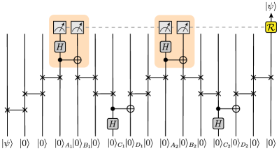
Figure 1: The entanglement-swapping teleportation protocol (ESTP) is illustrated for $L=15$, $T=4$, and $M=2$ (gate notation Barenco et al. (1995) is reviewed in the SM sup ). Bell pairs are generated on neighboring $C$ and $D$ qubits via a Hadamard–CNOT sequence ($\mathcal{B}$) and transported to $A$ and $B$ qubits via SWAP gates. The shaded areas indicate the standard teleportation protocol (STP) and include two $Z$ measurements each; the dashed line denotes classical communication. The logical qubit $\lvert\psi\rangle$ starts at $j=1$ and teleports to $j=16$ after applying the error-correction gate $\mathcal{R}$, which is determined by the measurement outcomes according to Tab. 1.

We now consider the ESTP in detail. The chain is divvied into $M$ repeating regions of size $\ell=2(T-1)$, along with $T-1$ qubits (including the initial logical qubit) to the left of the first region, and one or two qubits (including the target site) to the right of the last region. The first layers of $\mathcal{W}$ create Bell pairs on neighboring $C^{\,}_{s}$ and $D^{\,}_{s}$ qubits from the computational-basis state (11) via the “Bell encoding” channel $\mathcal{B}^{\,}_{s}=\operatorname{CNOT}(C^{\,}_{s}\rightarrow D^{\,}_{s})H^{\,}_{\small C^{\,}_{s}}$ Nielsen and Chuang (2010) on the neighboring $C$ and $D$ qubits in each region $s$. The SWAP gates then send $\lvert\psi\rangle$ to $A^{\,}_{1}$, $C^{\,}_{s}$ to $B^{\,}_{s}$, and $D^{\,}_{s}$ to $A^{\,}_{s+1}$, with $A^{\,}_{M+1}\equiv N$ the final site. The state is then

$$\lvert\Psi^{\,}_{t}\rangle\,=\,\lvert\psi\rangle^{\,}_{A^{\,}_{1}}\otimes\left[\bigotimes\limits_{s=1}^{M}\,\lvert\mathrm{Bell}\rangle^{\vphantom{\prime}}_{B^{\,}_{s}A^{\,}_{s+1}}\right]\otimes\lvert\Phi\rangle^{\,}_{\mathrm{rest}},$$ (12)

immediately before the orange regions in Fig. 1, where $\lvert\Phi\rangle^{\,}_{\mathrm{rest}}$ is a decoupled state of all other qubits.

The next step applies the STP to neighboring $A$ and $B$ qubits, indicated by the orange-shaded boxes of Fig. 1. First, the “Bell decoding” channel $\mathcal{B}^{\dagger}_{s}=H^{\,}_{\small A^{\,}_{s}}\operatorname{CNOT}(A^{\,}_{s}\rightarrow B^{\,}_{s})$ Nielsen and Chuang (2010) acts on neighboring $A$ and $B$ qubits in each of the $M\sim N/T$ regions $s$. Next, the outcomes of measuring $Z^{\vphantom{*}}_{A^{\,}_{s}}$ and $Z^{\vphantom{*}}_{B^{\,}_{s}}$ are recorded, which will determine the error-correcting unitary $\mathcal{R}$ to apply to the final site. Bell decoding ensures that the measurements in the nonunitary channel $\mathsf{M}$ (indicated by pointer dials in Fig. 1) are in the computational ($Z^{\vphantom{*}}$) basis, but can be omitted if one can measure in the Bell basis instead.

To be precise, after applying $\mathsf{M}^{\,}_{1}$ to $\left(A^{\,}_{1},B^{\,}_{1}\right)$ we find

$$\mathsf{M}^{\vphantom{\dagger}}_{1}\lvert\Psi^{\,}_{t}\rangle=\left(\mathcal{R}^{\,}_{1}\lvert\psi\rangle\right)^{\,}_{A^{\,}_{2}}\otimes\left[\bigotimes\limits_{s=2}^{M}\,\lvert\mathrm{Bell}\rangle^{\vphantom{\prime}}_{B^{\,}_{s}A^{\,}_{s+1}}\right]\otimes\lvert\Phi\rangle^{\,}_{\mathrm{rest}}\,,$$ (13)

where the gate $\mathcal{R}^{\,}_{1}\in\{\mathds{1},X,Y,Z\}$ depends on the outcomes of $\mathsf{M}^{\,}_{1}$. At this stage, the logical state $\lvert\psi\rangle$ has been teleported a distance $2(T-1)$ from site $A^{\,}_{1}$ to site $A^{\,}_{2}$.

This procedure is then repeated for the remaining regions $s=2,\dots,M$, collapsing the state $\lvert\Psi^{\,}_{t}\rangle$ onto one of the measurement outcomes,

$$\mathsf{M}\mathcal{B}^{\dagger}\lvert\Psi^{\,}_{t}\rangle\,=\,\lvert\Phi\rangle^{\,}_{1\cdots N-1}\otimes(\mathcal{R}\lvert\psi\rangle)^{\,}_{N}\,=\,\mathcal{R}\lvert\Psi^{\,}_{f}\rangle\,,~{}~{}$$ (14)

where $\lvert\Psi^{\,}_{f}\rangle$ is the desired final state, $\lvert\Phi\rangle$ is an arbitrary many-body state on sites $j\neq N$, and $\mathcal{R}$ is a single-site “error-correction” unitary, determined by the measurement outcomes (communicated instantaneously via the dashed lines in Fig. 1) according to Tab. 1.

$\;\;\mathcal{R}\;\;$	Measurement Outcomes
	$\quad\quad m^{\vphantom{\prime}}_{A}\quad\quad$	$m^{\vphantom{\prime}}_{B}$
$\mathds{1}$	1	1
$X$	1	-1
$Y$	-1	-1
$Z$	-1	1

Table 1: A “lookup” table for the local rotation $\mathcal{R}$ is given for the various measurement outcomes. Here $m^{\,}_{A},m^{\,}_{B}$ denote the product of $Z$-measurement outcomes on the qubits in sets $A$ and $B$, respectively.

Specifically, $\mathcal{R}=\prod_{s=1}^{M}\mathcal{R}^{\,}_{s}$ is determined by the product of measurement outcomes for the $A$ and $B$ sites (see Tab. 1). Applying $\mathcal{R}$ to (14) on the final site “undoes” the error, giving $\lvert\Psi^{\,}_{f}\rangle$ with the logical state $\lvert\psi\rangle$ on the final site $j=N$. In this way, the ESTP enhances the standard teleportation protocol with SWAP gates and daisy-chained Bell pairs to cover more distance. The distance $L$ over which the ESTP teleports the logical state $\lvert\psi\rangle$ obeys (1), and more specifically, (48).

2.3 Logical operator dynamics

An alternative perspective to the Schrödinger dynamics of states is afforded by the Heisenberg dynamics of the logical operators—unitary operators that reproduce the Pauli algebra acting on $\lvert\psi\rangle$. One choice of logical operators for the final state $\lvert\Psi^{\,}_{f}\rangle$ (14) corresponds to

$$X^{\vphantom{*}}_{{\rm L}}\,=\,X^{\vphantom{*}}_{N}\,,~{}~{}Z^{\vphantom{*}}_{{\rm L}}\,=\,Z^{\vphantom{*}}_{N}\,,~{}\,\text{with}\,~{}Y^{\vphantom{*}}_{{\rm L}}\,=\,\mathrm{i}X^{\vphantom{*}}_{{\rm L}}Z^{\vphantom{*}}_{{\rm L}}\,,~{}~{}$$ (15)

and we now evolve these logical operators forward in the Heisenberg picture—corresponding to backward time evolution in the Schrödinger picture—to recover their action on the initial state (11),

$$O(T)\, =\,\mathcal{W}^{\dagger}\mathcal{B}\mathsf{M}^{\dagger}\mathcal{R}^{\dagger}\,O(0)\,\mathcal{R}\mathsf{M}\mathcal{B}^{\dagger}\mathcal{W}\,,~{}~{}$$ (16)

where the channel $\mathsf{M}=\mathsf{M}^{\,}_{A}\mathsf{M}^{\,}_{B}$ encodes the single-site measurements of $Z^{\vphantom{*}}$ on the $A$ and $B$ qubits. The Heisenberg evolution of the logical operator $X^{\vphantom{*}}_{{\rm L}}=X^{\vphantom{*}}_{N}$ for the ESTP depicted in Fig. 1 is illustrated in Fig. 2.

Acting on states, $\mathsf{M}^{\,}_{A}$ determines $m^{\,}_{A}=(-1)^{N^{\,}_{A}}$ with $N^{\,}_{A}$ the number of $A$ sites in the state $\lvert 1\rangle$, and likewise for $m^{\,}_{B}$; the error-correction channel $\mathcal{R}$ is determined by $m^{\,}_{A,B}$ according to Tab. 1. As a channel on the physical Hilbert space, $\mathsf{M}$ is nonunitary, so some care is required to incorporate the effect of measurements.

Crucially, in the Heisenberg picture, the first channel applied to $O(0)$ in (16) corresponds to the error-correction channel $\mathcal{R}$ (i.e., conjugation of $O(0)$ by $\mathcal{R}=\mathcal{R}^{\,}_{A}\mathcal{R}^{\,}_{B}$). The unitary $\mathcal{R}^{\,}_{A}$ acts as $Z^{\vphantom{*}}_{N}$ if $m^{\,}_{A}=-1$, and $\mathcal{R}^{\,}_{B}$ acts as $X^{\vphantom{*}}_{N}$ if $m^{\,}_{B}=-1$ (and both $\mathcal{R}^{\,}_{A,B}$ act trivially otherwise). Since the overall sign of the wavefunction is not physically significant, the ordering of $\mathcal{R}^{\,}_{A}$ and $\mathcal{R}^{\,}_{B}$ in $\mathcal{R}$ is inconsequential. Conjugating the logical operators by $\mathcal{R}$ gives

$$\mathcal{R}^{\dagger}X^{\vphantom{*}}_{N}\mathcal{R}\,=\,m^{\,}_{A}\,X^{\vphantom{*}}_{N}\,,~{}\quad~{}\mathcal{R}^{\dagger}Z^{\vphantom{*}}_{N}\mathcal{R}\,=\,m^{\,}_{B}\,Z^{\vphantom{*}}_{N}\,.~{}~{}$$ (17)

Next, conjugation by the measurement channel $\mathsf{M}^{\,}_{A/B}$ acts nontrivially on the outcome $m^{\,}_{A/B}$ according to

$$m^{\,}_{A/B}\,\to\,Z^{\vphantom{*}}_{A/B}=\prod_{j\in A/B}\,Z^{\vphantom{*}}_{j}\,,~{}~{}$$ (18)

and does nothing to $m^{\,}_{B/A}$. We derive this update in Sec. 3 using the Stinespring Dilation Theorem Stinespring (1955); Choi (1975); Friedman et al. (2022) to represent measurements unitarily by appending qubits to record their outcomes (see also SM sup ). A similar update rule was derived in Chung et al. (2009); our perspective generalizes to arbitrary non-Clifford dynamics. We find

$$\mathsf{M}^{\dagger}\mathcal{R}^{\dagger}\,X^{\vphantom{*}}_{N}\,\mathcal{R}\mathsf{M}\, =\,X^{\vphantom{*}}_{N}Z^{\vphantom{*}}_{A}\,$$ (19a)

$$\mathsf{M}^{\dagger}\mathcal{R}^{\dagger}\,Z^{\vphantom{*}}_{N}\,\mathcal{R}\mathsf{M}\, =\,Z^{\vphantom{*}}_{N}Z^{\vphantom{*}}_{B}\,,~{}~{}$$ (19b)

and note that the generation of $Z^{\vphantom{*}}_{A,B}$ in the step above is crucial, and only occurs if $\mathcal{R}$ depends on $m^{\,}_{A,B}$.

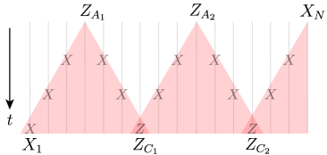
Figure 2: Heisenberg picture of the logical operator $X^{\,}_{\rm L}$ for the ESTP depicted in Fig. 1. The local $Z$ operators grow with Lieb-Robinson velocity $v=1$, as depicted by the edges of the shaded cones. The check operators during the intermediate steps are shown inside their respective “light cones.”

We next conjugate by $\mathcal{B}$, giving

$$X^{\vphantom{*}}_{{\rm L}}\to X^{\vphantom{*}}_{A}X^{\vphantom{*}}_{B}X^{\vphantom{*}}_{N}~{},~{}~{}~{}~{}Z^{\vphantom{*}}_{{\rm L}}\to Z^{\vphantom{*}}_{A}Z^{\vphantom{*}}_{B}Z^{\vphantom{*}}_{N}\,,~{}~{}$$ (20)

and applying the SWAP gates in $\mathcal{W}$ in reverse order moves the states of sites $A^{\,}_{1}\to 1$, $A^{\,}_{s}\to D^{\,}_{s-1}$ for $s>1$, $N\to D^{\,}_{M}$, and $B^{\,}_{s}\to C^{\,}_{s}$ for all $1\leq s\leq M$. The result is

$$X^{\vphantom{*}}_{{\rm L}}\to X^{\vphantom{*}}_{1}X^{\vphantom{*}}_{C}X^{\vphantom{*}}_{D}~{},~{}~{}~{}~{}Z^{\vphantom{*}}_{{\rm L}}\to Z^{\vphantom{*}}_{1}Z^{\vphantom{*}}_{C}Z^{\vphantom{*}}_{D}\,,~{}~{}$$ (21)

and applying $\mathcal{B}^{\dagger}$ to the $C,D$ sites gives

$$X^{\vphantom{*}}_{{\rm L}}(T)\,=\,X^{\vphantom{*}}_{1}\,Z^{\vphantom{*}}_{C}\,,~{}\quad~{}Z^{\vphantom{*}}_{{\rm L}}(T)\,=\,Z^{\vphantom{*}}_{1}\,Z^{\vphantom{*}}_{D}\,,~{}~{}$$ (22)

for the initial logical operators, as shown in Fig. 2. Thus,

$$X^{\vphantom{*}}_{{\rm L}}(T)\,\lvert\Psi^{\,}_{0}\rangle\, =\,(X^{\vphantom{*}}\lvert\psi\rangle)^{\vphantom{\prime}}_{1}\otimes\lvert\mathbf{0}\rangle^{\vphantom{\prime}}_{2\cdots N},$$ (23a)

$$Z^{\vphantom{*}}_{{\rm L}}(T)\,\lvert\Psi^{\,}_{0}\rangle\, =\,(Z^{\vphantom{*}}\lvert\psi\rangle)^{\vphantom{\prime}}_{1}\otimes\lvert\mathbf{0}\rangle^{\vphantom{\prime}}_{2\cdots N}\,,~{}~{}$$ (23b)

as required for logical operators of the initial state (11).

Crucially, if $\mathcal{R}$ did not depend on the measurement outcomes, Heisenberg evolution would not successfully transfer the logical operator from site $j=N$ to site $j=1$. Equivalently, in the Schrödinger picture, no useful quantum information is teleported to qubit $j=N$ until the measurement outcomes are communicated and errors corrected (via $\mathcal{R}$). As in the STP, prior to application of $\mathcal{R}$ to site $j=N$, the outcome-averaged state is the maximally mixed state $\rho^{\,}_{f}=\mathds{1}/2$ (a random classical bit).

3 Measurement channels

The protocols we consider combine unitary time evolution and projective measurements to achieve useful quantum tasks. Note that the bound (1) extends to generic local quantum channels, as we explain in Sec. 4.7. All quantum channels can be described using three equivalent representations: completely positive trace-preserving (CPTP) maps, Kraus operators (which are equivalent to CPTP maps), and isometries Stinespring (1955); Choi (1975); Friedman et al. (2022); Barberena and Friedman (2023). The latter results from the Stinespring Dilation Theorem Stinespring (1955), and its equivalence to the other two representations follows from Choi’s Theorem Choi (1975). As we explain in Sec. 3.3, we exclusively consider the outcome-averaged density matrix, since individual trajectories have no bearing on any useful quantum task. In the Stinespring picture, this corresponds to tracing out the detector degrees of freedom.

3.1 Dilation Theorem and isometric measurement

The Stinespring Dilation Theorem Stinespring (1955) states that quantum channels can be represented using isometries and partial traces. An isometry is a length-preserving map from some physical Hilbert space $\mathcal{H}^{\,}_{\rm ph}$ (with dimension $\mathcal{D}^{\,}_{\rm ph}$) to some dilated Hilbert space $\mathcal{H}^{\,}_{\rm dil}$ (with dimension $\mathcal{D}^{\,}_{\rm dil}\geq\mathcal{D}^{\,}_{\rm ph}$). In particular, the isometries representing projective measurements have a unique form Barberena and Friedman (2023), in which the extra degrees of freedom in $\mathcal{H}^{\,}_{\rm dil}$ encode the outcome of the measurement. For the Pauli measurements of interest, the binary outcomes $n=0,1$ are stored in qubits.

We stress that the Stinespring Theorem Stinespring (1955) establishes that all nonunitary quantum channels are captured by partial traces and/or isometries (which involve ancillary “Stinespring” degrees of freedom). Weak and generalized measurements—as well as projective measurements with more than two outcomes—are all captured by this formalism. Surprisingly, even the measurement of unbounded operators (e.g., homodyne measurements and photon counting) are also captured via isometries Barberena and Friedman (2023).

While all of these cases are associated with distinct isometric channels, the locality properties of these channels are always the same. In particular, these isometries all couple a local region of qubits to ancillary Stinespring qubits, where the latter may be nonlocally accessed via instantaneous classical communication. Hence, the results we derive for projective measurements apply to generic nonunitary quantum channels (e.g., weak measurements).

For convenience of presentation, we consider the measurement of Pauli-string operators $\mathcal{O}$, which act on every site as one of the Pauli matrices or the identity (e.g., $X^{\vphantom{*}}_{i}$, $Z^{\vphantom{*}}_{i}$, $Z^{\vphantom{*}}_{i}Z^{\vphantom{*}}_{j}$, $Z^{\vphantom{*}}_{j-1}X^{\vphantom{*}}_{j}Z^{\vphantom{*}}_{j+1}$, etc.). The Pauli strings $\mathcal{O}$ satisfy $\mathcal{O}^{2}=\mathds{1}$, and their eigenvalues are $\pm 1$. It is convenient to write the spectral decomposition of $\mathcal{O}$,

$$\mathcal{O}\equiv\sum\limits_{\pm}\,\pm P^{(\pm)}_{\,}\,,~{}~{}P^{(\pm)}_{\,}\equiv\frac{1}{2}\left(\mathds{1}\pm\mathcal{O}\right)\,,~{}~{}$$ (24)

where the $\pm$ eigenvalues of $\mathcal{O}$ have degeneracy $2^{l-1}$ if $\mathcal{O}$ acts nontrivially on $l$ sites. We identify the label 0 with the $+1$ eigenvalue, and the label 1 with the $-1$ eigenvalue.

The eigenprojectors $P^{(n)}_{\,}$ for $n\in\{0,1\}$ satisfy

$$\mathcal{O}\,P^{(n)}_{\,}=(-1)^{n}\,P^{(n)}_{\,}\,,~{}~{}$$ (25)

and are orthonormal and idempotent, satisfying

$$P^{(m)}_{\,}P^{(n)}_{\,}=\delta^{\,}_{m,n}P^{(m)}_{\,}~{}~{}~{}\text{and}~{}~{}~{}\sum\limits_{n=0,1}\,P^{(n)}_{\,}=\mathds{1}\,,~{}~{}$$ (26)

where the labels $m,n\in\{0,1\}$.

If the observable $\mathcal{O}$ (24) is measured in the state $\lvert\psi\rangle\in\mathcal{H}^{\,}_{\rm ph}$ of the physical system, the post-measurement state $\lvert\psi^{\prime}\rangle$ in the Stinespring picture is given by

$$\lvert\psi\rangle\to\lvert\psi^{\prime}\rangle=\sum\limits_{n=0,1}\,\left(P^{(n)}_{\,}\lvert\psi\rangle\right)^{\vphantom{\dagger}}_{\rm ph}\otimes\lvert n\rangle^{\vphantom{\dagger}}_{\rm ss}\,,~{}~{}$$ (27)

where $\lvert\psi^{\prime}\rangle\in\mathcal{H}^{\,}_{\rm dil}$ lies in the dilated Hilbert space,

$$\mathcal{H}^{\vphantom{\prime}}_{\rm dil}=\mathcal{H}^{\vphantom{\prime}}_{\rm ph}\otimes\mathcal{H}^{\vphantom{\prime}}_{\rm ss}\,,~{}~{}$$ (28)

where in (27), the qubit in the state $\lvert n\rangle\in\mathcal{H}^{\,}_{\rm ss}$ records the observed outcome $n$, and $P^{(n)}_{\,}\lvert\psi\rangle$ is the post-measurement state of the physical system. The Stinespring states $\{\lvert 0\rangle,\lvert 1\rangle\}$ form a complete, orthonormal qubit basis, with $\left\langle m\middle|n\right\rangle=\delta^{\,}_{m,n}$ and $\widetilde{\mathds{1}}^{\vphantom{*}}=\lvert 0\rangle\langle 0\rvert+\lvert 1\rangle\langle 1\rvert$, where the tilde denotes an operator acting on $\mathcal{H}^{\,}_{\rm ss}\subset\mathcal{H}^{\,}_{\rm dil}$ (28).

The isometric channel $\mathbb{V}$ that represents the measurement process in (27) extends (or “dilates”) the physical Hilbert space $\mathcal{H}^{\,}_{\rm ph}$ to $\mathcal{H}^{\,}_{\rm dil}$ according to

$$\mathbb{V}^{\vphantom{\dagger}}_{[\mathcal{O}]}=\sum\limits_{n=0,1}\,P^{(n)}_{\rm ph}\otimes\lvert n\rangle^{\vphantom{\dagger}}_{\rm ss}\,,~{}~{}$$ (29)

where the outcome qubit (or “Stinespring register”) does not exist prior to application of the channel $\mathbb{V}$. Isometries are length preserving (i.e., $\mathbb{V}^{\dagger}\mathbb{V}=\mathds{1}$), so the state $\lvert\psi^{\prime}\rangle$ (27) remains normalized as written (27).

The probability to observe outcome $n\in\{0,1\}$ is

$$p^{\vphantom{\prime}}_{n}=\left\langle\psi^{\prime}\middle|\,\mathds{1}^{\vphantom{\prime}}_{\rm ph}\otimes\lvert n\rangle\langle n\rvert^{\vphantom{\prime}}_{\rm ss}\,\middle|\psi^{\prime}\right\rangle=\left\langle\psi\middle|P^{(n)}_{\rm ph}\middle|\psi\right\rangle\,,~{}~{}$$ (30)

and the expectation value of $\mathcal{O}$ (24) is given by

$$\langle\mathcal{O}\rangle^{\vphantom{\prime}}_{\psi} =\left\langle*\middle|\psi^{\prime}\middle|\,\sum\limits_{n=0,1}\,(-1)^{n}\lvert n\rangle\langle n\rvert^{\vphantom{\prime}}_{\rm ss}\,\right\rangle{\psi^{\prime}}\,,~{}~{}$$ (31)

and we see that both the probability for outcome $n$ (30) and expectation value of $\mathcal{O}$ (31) are extracted via operations on the Stinespring register.

3.2 Unitary measurement

However, the Stinespring Theorem Stinespring (1955) and isometric representation of channels on their own are not sufficient for the derivation of (1). Importantly, in the case where $\mathcal{D}^{\,}_{A}=\mathcal{D}^{\,}_{B}$, the corresponding isometric channel is unitary. The crucial insight here—and in the accompanying works Barberena and Friedman (2023); Friedman et al. (2022)—is the recognition that the extra Stinespring degrees of freedom in $\mathcal{H}^{\,}_{\rm dil}$ (but not in $\mathcal{H}^{\,}_{\rm ph}$) are physical. In the case of measurements, they reflect the state of the measurement apparatus; for other quantum channels, they represent environmental degrees of freedom. In this sense, the Stinespring qubits are physical (and not merely a bookkeeping device). Importantly, because an isometry from a Hilbert space to itself is unitary, any isometry can be embedded in a unitary operator by extending the dimension of the initial Hilbert space.

Thus, a unitary representation of measurement recovers by including Stinespring degrees of freedom from the outset, which we initialize in some default state. In other words, we work at all times in the dilated Hilbert space $\mathcal{H}^{\,}_{\rm ph}\to\mathcal{H}^{\,}_{\rm dil}$, which includes the Stinespring (i.e., “outcome” or “apparatus”) qubits for all possible measurements (e.g., in adaptive protocols where the choice of measurements may be conditioned on past outcomes). The resulting representation of all generic quantum channels, measurements, and outcome-dependent operations is unitary Friedman et al. (2022); Everett (1956); Barberena and Friedman (2023); sup , and corresponds to (discrete) time evolution of the system and measurement apparatus (or environment, more generally) under some particular entangling interaction. The fact that the unitary Stinespring representation of generic quantum channels corresponds to the physical time evolution of a larger, closed system is what allows for the Heisenberg evolution of operators in the presence of generic quantum channels.

As in Sec. 3.1, we restrict to systems of qubits and projective measurements of Pauli-string operators, so that the two outcomes are labelled 0 and 1. By convention, we initialize all Stinespring (or “outcome”) qubits in the state $\lvert 0\rangle$, and denote the product of all Stinespring qubits in this state by $\lvert\mathbf{0}\rangle^{\,}_{\rm ss}$. In Sec. 4.7 we explain how the results for projective measurements extend to generic, local quantum channels (e.g., weak measurements).

	$\left[\mathcal{O},\,A\right]=0$	$\left\{\mathcal{O},\,A\right\}=0$
$\widetilde{A}=\widetilde{\mathds{1}}^{\vphantom{*}}_{\,}$	$A\otimes\widetilde{\mathds{1}}^{\vphantom{*}}_{\,}$	$A\otimes\widetilde{X}^{\vphantom{*}}_{\,}$
$\widetilde{A}=\widetilde{X}^{\vphantom{*}}_{\,}$	$A\otimes\widetilde{X}^{\vphantom{*}}_{\,}$	$A\otimes\widetilde{\mathds{1}}^{\vphantom{*}}_{\,}$
$\widetilde{A}=\widetilde{Y}^{\vphantom{*}}_{\,}$	$A\,\mathcal{O}\otimes\widetilde{Y}^{\vphantom{*}}_{\,}$	$\mathrm{i}\,A\,\mathcal{O}\otimes\widetilde{Z}^{\vphantom{*}}_{\,}$
$\widetilde{A}=\widetilde{Z}^{\vphantom{*}}_{\,}$	$A\,\mathcal{O}\otimes\widetilde{Z}^{\vphantom{*}}_{\,}$	$-\mathrm{i}\,A\,\mathcal{O}\otimes\widetilde{Y}^{\vphantom{*}}_{\,}$
$\widetilde{A}=\widetilde{P}^{\,}_{\pm}$	$\,\frac{1}{2}A\left(\mathds{1}\otimes\widetilde{\mathds{1}}^{\vphantom{*}}_{\,}\pm\mathcal{O}\otimes\widetilde{Z}^{\vphantom{*}}_{\,}\right)\,$	$\,\frac{1}{2}A\left(\mathds{1}\otimes\widetilde{X}^{\vphantom{*}}_{\,}\mp\mathrm{i}\mathcal{O}\otimes\widetilde{Y}^{\vphantom{*}}_{\,}\right)\,$

Table 2: “Lookup” table for the values of $\mathsf{V}^{\,}_{[\mathcal{O}]}\,A\otimes\widetilde{A}\,\mathsf{V}^{\dagger}_{\left[\mathcal{O}\right]}$ (34), which corresponds to unitary measurement of observable $\mathcal{O}$ in either the Heisenberg (observable) or Schrödinger picture (density matrix). The operator $A\otimes\widetilde{A}$ acts as $A$ on the physical Hilbert space and as $\widetilde{A}$ on the Stinespring register that stores the outcome of measuring $\mathcal{O}$. The Pauli string $\mathcal{O}$ acts on each site $j$ as either $\mathds{1}$, $X^{\,}_{j}$, $Y^{\,}_{j}$, $Z^{\,}_{j}$; we decompose $A$ in this basis, so that $\mathcal{O}$ and $A$ either commute or anticommute.

The unitary operator describing the projective measurement of a Pauli-string operator $\mathcal{O}^{\,}_{n}$ is given by

$$\mathsf{V}^{\vphantom{\dagger}}_{\left[\mathcal{O}^{\,}_{n}\right]} \equiv\frac{1}{2}\left(\mathds{1}+\mathcal{O}^{\,}_{n}\right)\widetilde{\mathds{1}}^{\vphantom{*}}_{n}+\frac{1}{2}\left(\mathds{1}-\mathcal{O}^{\,}_{n}\right)\widetilde{X}^{\vphantom{*}}_{n}\,,~{}~{}$$ (32)

where the parenthetical terms act on the physical Hilbert space and the twiddled operators act on the $n$th Stinespring qubit. The second term flips the default outcome $\lvert 0\rangle$ to $\lvert 1\rangle$ when the $-1$ eigenstate of $\mathcal{O}^{\,}_{n}$ is observed Friedman et al. (2022).

The advantage of our Stinespring representation of measurement via unitary channels (32) is that it allows us to evolve operators. Note that the measurement unitary (32) is also Hermitian, so the evolution of density matrices and operators—in the Schrödinger and Heisenberg pictures, respectively—is equivalent, given by Friedman et al. (2022)

$$A^{\prime}_{\rm ph}\otimes\widetilde{A}^{\prime}_{\rm ss} =\mathsf{V}^{\vphantom{\dagger}}_{\left[\mathcal{O}\right]}\,A^{\vphantom{\prime}}_{\rm ph}\otimes\widetilde{A}^{\vphantom{\prime}}_{\rm ss}\mathsf{V}^{\dagger}_{\left[\mathcal{O}\right]}$$

$$=\mathsf{V}^{\dagger}_{\left[\mathcal{O}\right]}\,A^{\vphantom{\prime}}_{\rm ph}\otimes\widetilde{A}^{\vphantom{\prime}}_{\rm ss}\mathsf{V}^{\vphantom{\dagger}}_{\left[\mathcal{O}\right]}\,,~{}~{}$$ (33)

where the two pictures are only equivalent for qubits. Using (32), the channel (33) takes the form

$$=\frac{1}{4}\left\{\mathcal{O},\,A\right\}\mathcal{O}\otimes\left\{\widetilde{A},\,\widetilde{X}^{\vphantom{*}}\right\}\widetilde{X}^{\vphantom{*}}+\frac{1}{4}\left\{\mathcal{O},\,A\right\}\otimes\left[\widetilde{A},\,\widetilde{X}^{\vphantom{*}}\right]\widetilde{X}^{\vphantom{*}}$$

$$~{}-\frac{1}{4}\,\left[\mathcal{O},\,A\right]\,\mathcal{O}\otimes\left\{\widetilde{A},\,\widetilde{X}^{\vphantom{*}}\right\}+\frac{1}{4}\left[\mathcal{O},\,A\right]\otimes\left[\widetilde{A},\,\widetilde{X}^{\vphantom{*}}\right]\,,$$ (34)

which we summarize in Tab. 2. Note that for density matrices, $\widetilde{A}$ is generally a projector $\lvert 0\rangle\langle 0\rvert^{\,}_{\rm ss}=(\widetilde{\mathds{1}}^{\vphantom{*}}+\widetilde{Z}^{\vphantom{*}})/2$, while for observables, $\widetilde{A}$ is generally the identity $\widetilde{\mathds{1}}^{\vphantom{*}}$.

3.3 Trajectories and expectation values

By convention, $\varrho$ denotes density matrices in the dilated Hilbert space (28), with the initial state given by

$$\varrho(0)\equiv\rho\otimes\lvert\boldsymbol{0}\rangle\langle\boldsymbol{0}\rvert^{\,}_{\rm ss}\,,~{}~{}$$ (35)

where $\lvert\boldsymbol{0}\rangle\langle\boldsymbol{0}\rvert^{\,}_{\rm ss}=\bigotimes_{j=1}^{M}\lvert 0\rangle\langle 0\rvert^{\,}_{{\rm ss},j}$ initializes all Stinespring registers in the default state $\lvert 0\rangle$ and $\rho$ is the initial density matrix for the physical system. This state is then evolved under a hybrid protocol $\mathcal{W}\in\operatorname{End}(\mathcal{H}^{\,}_{\rm dil})$ to produce

$$\varrho(t)=\mathcal{W}^{\vphantom{\dagger}}\varrho(0)\mathcal{W}^{\dagger}\,,~{}~{}$$ (36)

and assuming $\mathcal{W}$ contains a single measurement of some generic (many-body) observable $\mathcal{O}$ (24), the probability to obtain outcome $n$ is given by

$$p^{\vphantom{\prime}}_{n}=\operatorname*{tr}\limits_{\rm dil}\,\left[\,\mathds{1}^{\vphantom{\dagger}}_{\rm ph}\otimes\lvert n\rangle\langle n\rvert^{\vphantom{\dagger}}_{\rm ss}\,\varrho(t)\,\right]\,,~{}~{}$$ (37)

while the expectation value of $\mathcal{O}$ in the state (35) is

$$\langle\mathcal{O}\rangle^{\vphantom{\dagger}}_{\varrho}=\operatorname*{tr}\limits_{\rm dil}\,\left[\,\varrho(t)\,\sum\limits_{n=1}^{\mathcal{N}}\,\xi^{\vphantom{\prime}}_{n}\,\lvert n\rangle\langle n\rvert^{\vphantom{\dagger}}_{\rm ss}\,\right]\,,~{}~{}$$ (38)

where $\mathcal{N}$ is the number of unique eigenvalues (and thus, outcomes) of the measured observables $\mathcal{O}$.

More generally, the operator that projects onto the set of outcomes $\boldsymbol{n}\,=\,\{n^{\,}_{1},\dots,n^{\,}_{M}\}$ is simply

$$P^{\vphantom{\prime}}_{\boldsymbol{n}} \equiv P^{(\boldsymbol{n})}_{\rm ss}=\bigotimes\limits_{j\in{\rm ss}}\,\lvert n^{\,}_{j}\rangle\langle n^{\,}_{j}\rvert^{\vphantom{\prime}}_{{\rm ss},j}=\lvert\boldsymbol{n}\rangle\langle\boldsymbol{n}\rvert^{\,}_{\rm ss},~{}~{}$$ (39)

which acts nontrivially only on $\mathcal{H}^{\,}_{\rm ss}$, projecting the outcome qubit $j$ onto $n^{\,}_{j}\in\{0,1\}$. Note that the density matrix (36) projected onto trajectory $\boldsymbol{m}\subset\boldsymbol{n}$ (39) for a subset $\Omega\subset\mathcal{H}^{\,}_{\rm ss}$ requires renormalization:

$$\varrho^{\vphantom{\prime}}_{\boldsymbol{m}}(t) \equiv\operatorname*{tr}\limits_{\Omega}\,\left[\,P^{(\boldsymbol{m})}_{\Omega}\,\varrho(t)\,\right]/\operatorname*{tr}\limits_{\rm dil}\,\left[\,P^{(\boldsymbol{m})}_{\Omega}\,\varrho(t)\,\right]\,.~{}~{}$$ (40)

The probability to realize a particular sequence of measurement outcomes along the protocol $\mathcal{W}$ is defined in terms of the outcome projector (39) via

$$p^{\vphantom{\prime}}_{\boldsymbol{n}}={\rm tr}\left[\,\mathds{1}^{\vphantom{\dagger}}_{\rm ph}\otimes\lvert\boldsymbol{n}\rangle\langle\boldsymbol{n}\rvert^{\vphantom{\prime}}_{\rm ss}\,\varrho(t)\right]\,,~{}~{}$$ (41)

which can be evaluated part way through the protocol $\mathcal{W}$, provided that $n^{\,}_{i}=0$ for all $n^{\,}_{i}\in\boldsymbol{n}$ corresponding to measurements that have not yet occurred. Moreover, the joint and conditional expectation values of all observables are readily defined by implementing (38) for each observable; conditional expectation values utilize (40).

In deriving the bound (1), we exclusively consider the outcome-averaged density matrix (or evolution of operators). The physical rationale for this is simple: The bound (1) constrains useful quantum tasks, all of which output (i.e., either prepare or manipulate) a particular quantum state (in the form of a density matrix $\varrho$). Necessarily, that state is used to extract statistics and/or expectation values, which require numerous “shots” to resolve. Thus, in any experimental implementation, the statistics or expectation values always correspond to the state that the protocol prepares on average, since the repeated shots will sample over histories of outcomes. In this sense, the outcome-averaged density matrix is the effective output of any useful quantum task. In the case of a pure state $\rho$ of the physical system, the task must output $\rho$ for all outcomes; in the case of a mixed state $\rho$, the different outcomes realize the various pure states that comprise $\rho$ with the required coefficients (i.e., probabilities).

In the Stinespring formalism, for any protocol $\mathcal{W}$ involving time evolution, measurements, and outcome-dependent operations, the output density matrix

$$\rho^{\vphantom{\dagger}}_{\rm av}(t) =\operatorname*{tr}\limits_{\rm ss}\left[\mathcal{W}\,\rho^{\vphantom{\prime}}_{0}\otimes\lvert\boldsymbol{0}\rangle\langle\boldsymbol{0}\rvert^{\vphantom{\prime}}_{\rm ss}\,\mathcal{W}^{\dagger}\right]$$ (42)

is realized from the initial physical state $\rho^{\,}_{0}$ upon averaging over all outcomes (i.e., tracing out the Stinespring degrees of freedom is equivalent to averaging over outcomes).

3.4 Operator dynamics

Using the Stinespring formalism, we now consider the measurement-related aspects of the ESTP described in Sec. 2.2. The measurement channel $\mathsf{M}=\mathsf{M}^{\,}_{A}\,\mathsf{M}^{\,}_{B}$ further factorizes over the individual measurements, e.g.,

$$\mathsf{M}^{\vphantom{\dagger}}_{A}\,=\,\bigotimes\limits_{s=1}^{M}\,\frac{1}{2}\sum\limits_{n_{s}=0,1}\,\left(\mathds{1}+(-1)^{n_{s}}Z^{\vphantom{*}}_{A^{\,}_{s}}\right)\otimes\widetilde{X}^{n_{s}}_{A^{\,}_{s}}\,,~{}~{}$$ (43)

and likewise for $\mathsf{M}^{\,}_{B}$ (with $A\to B$ above). The individual measurement unitaries are equivalent to (32).

The error-correction channel $\mathcal{R}=\mathcal{R}^{\,}_{A}\,\mathcal{R}^{\,}_{B}$ is somewhat more subtle, and can be worked out from Tab. 1 and the Stinespring encoding of outcomes,

$$\mathcal{R}^{\vphantom{\dagger}}_{A}\, =\,\mathds{1}\otimes\frac{1}{2}\left(\widetilde{\mathds{1}}^{\vphantom{*}}+\widetilde{Z}^{\vphantom{*}}_{A}\right)+Z^{\vphantom{*}}_{N}\otimes\frac{1}{2}\left(\widetilde{\mathds{1}}^{\vphantom{*}}-\widetilde{Z}^{\vphantom{*}}_{A}\right)$$ (44a)

$$\mathcal{R}^{\vphantom{\dagger}}_{B}\, =\,\mathds{1}\otimes\frac{1}{2}\left(\widetilde{\mathds{1}}^{\vphantom{*}}+\widetilde{Z}^{\vphantom{*}}_{B}\right)+X^{\vphantom{*}}_{N}\otimes\frac{1}{2}\left(\widetilde{\mathds{1}}^{\vphantom{*}}-\widetilde{Z}^{\vphantom{*}}_{B}\right)\,,~{}~{}$$ (44b)

where $\widetilde{Z}^{\vphantom{*}}_{A/B}=\bigotimes_{j\in A/B}\,\widetilde{Z}^{\vphantom{*}}_{j}$ is a shorthand.

For clarity, we briefly reconsider the first steps in the evolution of the logical operators in Sec. 2.3. The first step corresponds to conjugation of the logical operators $X^{\vphantom{*}}_{{\rm L}}(0)$ and $Z^{\vphantom{*}}_{{\rm L}}(0)$ for the final state $\lvert\Psi^{\,}_{f}\rangle$ (15) by the error-correcting channel (44). We note that $\mathcal{R}^{\,}_{A}$ (44a) acts trivially on $Z^{\vphantom{*}}_{{\rm L}}(0)$, while $\mathcal{R}^{\,}_{B}$ (44b) acts trivially on $X^{\vphantom{*}}_{{\rm L}}(0)$. It is straightforward to verify the update

$$\mathcal{R}^{\dagger}_{A}\,X^{\vphantom{*}}_{{\rm L}}(0)\,\mathcal{R}^{\vphantom{\dagger}}_{A}\, =\,X^{\vphantom{*}}_{N}\,\widetilde{Z}^{\vphantom{*}}_{A}$$ (45a)

$$\mathcal{R}^{\dagger}_{B}\,Z^{\vphantom{*}}_{{\rm L}}(0)\,\mathcal{R}^{\vphantom{\dagger}}_{B}\, =\,Z^{\vphantom{*}}_{N}\,\widetilde{Z}^{\vphantom{*}}_{B}\,,~{}~{}$$ (45b)

where $\widetilde{Z}^{\vphantom{*}}_{A/B}$ replaces $m^{\,}_{A/B}$ in (17).

We next conjugate by the measurement channel, represented unitarily in the dilated Hilbert space. Similarly to the previous step, $\mathsf{M}^{\,}_{A}$ acts trivially on $\widetilde{Z}^{\vphantom{*}}_{B}$ (and vice versa). Hence, we need only consider the following updates,

$$\mathsf{M}^{\dagger}_{A}\,X^{\vphantom{*}}_{N}\,\widetilde{Z}^{\vphantom{*}}_{A}\,\mathsf{M}^{\vphantom{\dagger}}_{A}\, =\,Z^{\vphantom{*}}_{A}\,X^{\vphantom{*}}_{N}\,\widetilde{Z}^{\vphantom{*}}_{A}$$ (46a)

$$\mathsf{M}^{\dagger}_{B}\,Z^{\vphantom{*}}_{N}\,\widetilde{Z}^{\vphantom{*}}_{B}\,\mathsf{M}^{\vphantom{\dagger}}_{B}\, =\,Z^{\vphantom{*}}_{B}\,Z^{\vphantom{*}}_{N}\,\widetilde{Z}^{\vphantom{*}}_{B}\,,~{}~{}$$ (46b)

as claimed in (18). Since all measurements accounted for, we next simply evaluate the Stinespring operators in the default state $\lvert\boldsymbol{0}\rangle$ on all Stinespring qubits, so that

$$\left\langle*\middle|\boldsymbol{0}\middle|\widetilde{Z}^{\vphantom{*}}_{A/B}\right\rangle{\boldsymbol{0}}\,=\,1\,,~{}~{}$$ (47)

and the Stinespring operators in (46) vanish, reproducing (19). The remainder of the Heisenberg treatment of Sec. 2.3 does not require the Stinespring formalism.

We also refer the reader to the SM sup for the Stinespring treatment of another optimal teleportation protocol based on the transverse field Ising model Hong et al. (2022).

4 Lieb-Robinson Bounds

We now prove the bound (1), extending Lieb-Robinson bounds Lieb and Robinson (1972) to nonrelativistic quantum dynamics involving arbitrary local quantum channels (i.e., completely positive, trace-preserving maps) and instantaneous classical communication. In particular, we focus on the combination of unitary time evolution, projective measurements, and outcome-dependent local operations. We provide numerous application-specific bounds, and also prove that the bound (1) is optimal in a number of settings.

Absent measurements, (1) reduces to the usual bound $L\leq vT$ Lieb and Robinson (1972). In this sense, (1) also captures standard Lieb-Robinson bounds—in such cases we have $M^{\,}_{0}\leq 2$, which is saturated by, e.g., circuits with “light-cone” geometries. Importantly, (1) extends the standard Lieb-Robinson Theorem Lieb and Robinson (1972) to protocols $\mathcal{W}$ involving measurements in $M$ local regions. More formally, for an adaptive protocol $\mathcal{W}$, for each outcome “trajectory” $\boldsymbol{n}$, $\mathcal{W}$ prescribes measurements in local regions $S^{\,}_{k}$, from which we construct the set of regions $\mathbb{M}^{\,}_{\boldsymbol{n}}$ by appending the region of support $S^{\,}_{k}$ of the $k$th measurement to $\mathbb{M}^{\,}_{\boldsymbol{n}}$, unless $S^{\,}_{k}$ already appears in $\mathbb{M}^{\,}_{\boldsymbol{n}}$ or if $S^{\,}_{k}$ is a proper subset of some $S^{\,}_{j}\in\mathbb{M}^{\,}_{\boldsymbol{n}}$. Then, if no region $S^{\,}_{k}$ includes the initial task qubit $i$, we include a new region $S^{\,}_{-1}=\{i\}$; otherwise we relabel the region that includes $i$ as $S^{\,}_{-1}$. We similarly identify the region $S^{\,}_{0}$ with the task qubit $f$, and define $M$ as the maximum over all trajectories $\boldsymbol{n}$ of $\lvert\mathbb{M}^{\,}_{\boldsymbol{n}}\rvert-2$.

While in certain cases there is some freedom (i.e., ambiguity) in defining the measurement regions, especially in the limit $M=\mathsf{O}\left(L\right)$, one should generally pick the minimum value of $M$ possible. In the context of the ESTP, e.g., one can pick each $Z^{\vphantom{*}}$ measurement to represent a region; however, absorbing the Bell decoding channel into the measurements shows that it is possible to identify pairs of single-qubit measurements with a single region, in which case the task is optimal. This is also more transparent in the limit $M=\mathsf{O}\left(1\right)$. In general, any refinements to the definitions of $M$, $\mathcal{M}$, $M^{\,}_{0}$, and $T^{\,}_{0}$ are $\mathsf{O}\left(1\right)$ and depend on the particular protocol and/or task.

As noted in Sec. 3.3, we need only consider the reduced dynamics of the physical system, which corresponds to averaging over outcomes (42). In fact, (1) derives from considering the reduced density matrix $\rho^{\,}_{if}$ for the task qubits $i$ and $f$. All useful quantum tasks either generate, transfer, or manipulate quantum information, entanglement, and/or correlations. Hence, the output of any such task is always a quantum state $\varrho$, of which only the physical part is meaningful. Importantly, this state is subsequently utilized by extracting expectation values and/or statistics, which requires numerous experimental “shots.” As a result, the state that one samples in practice is the outcome-averaged output of the protocol, given by tracing over the Stinespring degrees of freedom (42). In the case of pure states, the same pure state must output for any sequence of outcomes; in the case of mixed states, the ratios in which the distinct pure states (that comprise the mixed state) appear is fixed by the mixed state itself. This also means that there is no reason to consider statistics over measurement outcomes, as they are trivial for pure states, and prescribed for mixed states.

We first consider Clifford circuits in Sec. 4.1, which are both simple and relevant to optimal protocols (e.g., the ESTP of Sec. 2). However, (1) also applies to more general dynamics generated by the combination of arbitrary, local, time-dependent Hamiltonians $H(t)$, and local quantum channels (e.g., projective or weak measurements and outcome-dependent operations). We give a physical explanation of the derivation of this bound in Sec. 4.2.

The full, rigorous proof is both lengthy and technical, and further details appear in the SM sup . Crucially, we need only assume that (i) the physical system comprises qubits on some physical graph $G$ with vertex set $V$, edges $E$, and spatial dimension $D$; (ii) the time-dependent Hamiltonian is a sum of local terms $H(t)=\sum_{j}H^{\,}_{j}(t)$ where $H^{\,}_{j}$ acts on finitely many sites neighboring $j$; (iii) the nonunitary quantum channels are spatially local; and (iv) that $T$ satisfies $vT\gtrsim 3$ or $H(t)$ generates a quantum circuit. In Secs. 4.6 and 4.7, we explain how this generalizes beyond qubits, nearest-neighbor Hamiltonians, and to generic local quantum channels.

In the SM sup we establish the equivalence of several useful tasks: For example, preparing a Bell state of two qubits separated by distance $L$ is equivalent to teleporting a state $\lvert\psi\rangle$ (6) by distance $L$, up to $\mathsf{O}\left(1\right)$ corrections to $T$, $M$, and the number of qubits (as realized by the standard teleportation protocol of Sec. 2.1). We also provide in the SM sup a straightforward proof that, e.g., teleportation of a state $\lvert\psi\rangle$ (6) from site $i$ to site $f$ is equivalent to moving the corresponding logical operators (15) from site $i$ to site $f$. This provides for the derivation of (1) in terms of operator dynamics, for which the unitary representation of quantum channels Friedman et al. (2022); Barberena and Friedman (2023) in Sec. 3 is crucial. We also note that the possibility of outcome-dependent operations applied instantaneously at arbitrary distances is incompatible with a Lieb-Robinson bound except using our unitary formalism—i.e., this would lead to completely nonlocal Lindblad operators, precluding the bound of Poulin (2010). Relatedly, a standard Lieb-Robinson bound does not apply to the dilated dynamics.

The bound (1) applies to “useful quantum tasks,” which transfer quantum information or generate entanglement (and/or correlations) over distance $L$. This includes, e.g., the preparation of generic many-body states in a region of size $L^{D}$, including the GHZ (3), quantum critical (4), W (5) Dür et al. (2000), Dicke Dicke (1954), and spin-squeezed Ma et al. (2011) states (see SM sup ). These bounds are derived in Sec. 4.3, and closely resemble (1). The main caveat is a small restriction on the compatible initial states, which we discuss in Sec. 4.5. We also prove that (1) cannot be sidestepped by teleporting multiple qubits in parallel, and detail applications of the bound (1) in Sec. 5. Note that protocols that do not teleport information or generate entanglement (and/or correlations) need not obey (1); conversely, protocols that violate (1) cannot be useful, as we illustrate.

4.1 Bounds for Clifford dynamics

We now prove (1) for Clifford protocols, such as the ESTP. Importantly, the local gates in a Clifford circuit always map Pauli strings (i.e., operators that act on every site as $\mathds{1}$, $X^{\vphantom{*}}$, $Y^{\vphantom{*}}$, or $Z^{\vphantom{*}}$) to Pauli strings. We restrict to single- and two-site Clifford gates, as is common practice. By convention, the time $T$ in (1) is the circuit depth, equal to the minimum number of layers required to implement all (physical) two-site gates, parallelizing where possible. Since only two-site gates “grow” operators—and by at most one site per gate—this counting gives $v=1$ in (1). Allowing for three-site and larger gates and/or altering the convention for $T$ simply modifies $v$; in general, $T$ should be thought of as the actual run time of the protocol.

We now justify the bound (1) in the presence of measurements, focusing on the teleportation of logical operators by the ESTP of Sec. 2 for convenience of presentation. Although we refer to projective measurements below, all statements apply equally to generic quantum channels (i.e., other than physical time evolution); as we clarify in Sec. 4.7. In general, we expect that only protocols combining time evolution, projective measurements, and outcome-dependent operations can saturate (1).

The proof of the bound (1) for Clifford circuits follows from, e.g., the fact that all deviations from the ESTP of Fig. 1 either (i) continue to saturate the bound (1) for a different task distance $L$, and are thus equivalent to the ESTP; (ii) achieve suboptimal teleportation and fail to saturate the bound (1); or (iii) fail to teleport the logical state entirely Hong et al. (2023a). Additionally, protocols that violate (1) cannot teleport information. The same arguments apply to preparing entangled (and/or correlated) resources states, as we discuss in Sec. 4.3; in Sec. 5, we present several optimal Clifford protocols that achieve other useful quantum tasks and saturate (1).

Note that successful teleportation requires that the logical operators $X^{\vphantom{*}}_{{\rm L}}(0)$ and $Z^{\vphantom{*}}_{{\rm L}}(0)$ (15)—which act as $X^{\vphantom{*}}_{N}$ and $Z^{\vphantom{*}}_{N}$ on the final state $\lvert\Psi^{\,}_{f}\rangle$ (14)—trivially commute except at $j=N$. The Heisenberg-evolved logical operators $X^{\vphantom{*}}_{{\rm L}}(T)$ and $Z^{\vphantom{*}}_{{\rm L}}(T)$ (22)—which act as $X^{\vphantom{*}}_{1}$ and $Z^{\vphantom{*}}_{1}$ on the initial state $\lvert\Psi^{\,}_{0}\rangle$ (11)—must act as $\mathds{1}$ or $Z$ (and thus commute) on all sites except $j=1$ to obey (23). We denote by $j_{*}(t)$ the rightmost site on which the operators $X^{\vphantom{*}}_{{\rm L}}(t)$ and $Z^{\vphantom{*}}_{{\rm L}}(t)$ anticommute, and require that $j_{*}(T)=1$. Furthermore, useful quantum tasks other than teleportation are also generically captured by the evolution of operators, and may be analogously constrained.

In the absence of measurements, the two-site Clifford gates (with $v=1$) can only decrease $j_{*}$ by one site per time step. In this scenario, teleporting $X^{\vphantom{*}}_{{\rm L}}(0)$ and $Z^{\vphantom{*}}_{{\rm L}}(0)$ from site $j=N$ to site $j=1$ requires $T\geq N-1=L$ circuit layers. This bound is saturated by a “staircase” of SWAP gates and agrees with (1) for $M=0$.

The ESTP depicted in Fig. 1 generalizes to other choices of $L,M,T$ by identifying $M$ repeating regions of size $\ell=2(T-1)$, along with an additional $T-2$ qubits to the left (including the initial logical site $j=1$) and a final qubit (or two) $j=N$ to the right. Then, the distance $L$ over which the ESTP teleports a qubit obeys

$$L^{\vphantom{\prime}}_{\small\rm ESTP}\,\leq\,\left(2\,M+1\right)\left(T-1\right)+1\,,~{}~{}$$ (48)

which saturates (1) with $M^{\,}_{0}=1$ and $T^{\,}_{0}=-1$. If one measures $X^{\vphantom{*}}_{j}X^{\vphantom{*}}_{j+1}$ and $Z^{\vphantom{*}}_{j}Z^{\vphantom{*}}_{j+1}$ instead of $Z^{\vphantom{*}}_{j}$ and $Z^{\vphantom{*}}_{j+1}$, then we find $L\leq(2M+1)T-1$, since the final layer of CNOT gates is no longer required. Importantly, this explains why the correct choice of “measurement regions” are pairs of neighboring qubits. Generally speaking, if a given protocol $\cal W$ obeys (1) with either $M^{\,}_{0}<0$ or $T^{\,}_{0}<0$, then a more efficient implementation of $\mathcal{W}$ exists.

Importantly, the ESTP transfers information with effective speed $v=2\,M+1$, compared to $v=1$ without measurements. Alternatively, one can view $(2M+1)T$ as the correct extension of the depth $T$ for $M>0$, compared to the standard Lieb-Robinson bound $L\leq vT$ when $M=0$ Lieb and Robinson (1972). Including extra layers of SWAP gates prior to the measurements grows the region size $\ell=2(T-1)$, so that the ESTP remains optimal with increased $T,L$; including additional measurement regions with the same $\ell$ also at best leaves the ESTP optimal with increased $M,L$. However, including other two-site Clifford gates generally leads to suboptimal teleportation with respect to (1). Any two-site gates applied after the measurement channel $\mathsf{M}$ have $v=1$ (compared to $v=2\,M+1$ for the ESTP on its own). Given $L^{\,}_{\small\rm ESTP}$ (48) for the ESTP, including $T^{\prime}$ layers of two-site gates at any point after the measurement channel $\mathsf{M}$ realizes a task distance

$$L^{\prime}\,\leq\,L^{\vphantom{\prime}}_{\small\rm ESTP}+T^{\prime}\,<\,2\,M\,(T+T^{\prime})\,,~{}~{}$$ (49)

which is suboptimal compared to (1). Hence, in optimal teleportation, the measurement channel $\mathsf{M}$ is applied after all two-site unitary channels to maximize $L$ (48).

We now prove that it is not possible to realize a greater enhancement to $v$ than $\left(2\,M+1\right)$ using measurements in $M$ regions. In step (19) of the Heisenberg evolution of the logical operators (15), the combination of the error-correction and measurement channels ($\mathcal{R}$ and $\mathsf{M}$) attaches the measured Pauli operators to $X^{\vphantom{*}}_{{\rm L}}(0)$ and $Z^{\vphantom{*}}_{{\rm L}}(0)$ at the corresponding measurement locations (as depicted at the top of Fig. 2), which may be arbitrarily far from the final site $j=N$. Importantly, this process (44) attaches distinct operators to the two distinct logical operators—i.e., $X^{\vphantom{*}}_{{\rm L}}\to Z^{\vphantom{*}}_{A}\,X^{\vphantom{*}}_{N}$ while $Z^{\vphantom{*}}_{{\rm L}}\to Z^{\vphantom{*}}_{B}\,Z^{\vphantom{*}}_{N}$. There are no further measurements with which to contend in the Heisenberg evolution of $X^{\vphantom{*}}_{{\rm L}}(t)$ and $Z^{\vphantom{*}}_{{\rm L}}(t)$, since optimal teleportation requires that measurements and error-correction occur after all unitaries to ensure that $v\sim 2M$ (49).

Importantly, we still have $j_{*}=N$ after step (19), but we require $j_{*}=1$ (23). Yet, there is no unitary operation that converts $X^{\vphantom{*}}_{N}$ to the identity, and converting $X^{\vphantom{*}}_{N}$ to $Z^{\vphantom{*}}_{N}$ also converts $Z^{\vphantom{*}}_{N}$ to $X^{\vphantom{*}}_{N}$, leaving $j_{*}$ unchanged. In fact, if the protocol does not utilize the Paulis seeded by the measurement channels in the step (19), the fastest way to realize $j_{*}=1$ (23) is to use $T=N-1=L$ layers of SWAP gates, in which case there is no enhancement due to the measurements! Thus, any advantage due to measurements must relate to the seeded Pauli operators.

While there is no means of removing a single $X^{\vphantom{*}}$ operator, step (22) shows that it is possible to convert both $X^{\vphantom{*}}_{j}X^{\vphantom{*}}_{j+1}$ and $Z^{\vphantom{*}}_{j}Z^{\vphantom{*}}_{j+1}$ into stabilizer operators compatible with (23). This is due to the fact that these two operators commute and share $\lvert\text{Bell}\rangle$ as a common eigenstate. Specifically, the Bell encoding (decoding) channel $\mathcal{B}^{(\dagger)}_{j,j+1}$ simultaneously converts $X^{\vphantom{*}}_{j}X^{\vphantom{*}}_{j+1}\leftrightarrow Z^{\vphantom{*}}_{j}$ and $Z^{\vphantom{*}}_{j}Z^{\vphantom{*}}_{j+1}\leftrightarrow Z^{\vphantom{*}}_{j+1}$. Applying these channels leads to $X^{\vphantom{*}}_{{\rm L}}(1)=X^{\vphantom{*}}_{A}X^{\vphantom{*}}_{B}X^{\vphantom{*}}_{N}$ and $Z^{\vphantom{*}}_{{\rm L}}(1)=Z^{\vphantom{*}}_{A}Z^{\vphantom{*}}_{B}Z^{\vphantom{*}}_{N}$ (20). Then, achieving $j_{*}=1$ requires that the $2M+1$ Pauli $X^{\vphantom{*}}$ operators in $X^{\vphantom{*}}_{{\rm L}}(1)$ be relocated (unitarily) such that one appears on site $j=1$ and all others are grouped into pairs on neighboring sites, as depicted in Fig. 2 for $X^{\vphantom{*}}_{{\rm L}}(t)$. This is most efficiently accomplished via the SWAP gates of the ESTP (see Fig. 1): The leftmost $X^{\vphantom{*}}$ and $Z^{\vphantom{*}}$ operators move to site $j=1$; the operators on site $B^{\,}_{s}$ move to site $C^{\,}_{s}$ of the same region, while the operator from site $A^{\,}_{s+1}$ moves to site $D^{\,}_{s}$ (where $A^{\,}_{M+1}=N$). Finally, the Bell encoding channel converts $X^{\vphantom{*}}_{C^{\,}_{s}}X^{\vphantom{*}}_{D^{\,}_{s}}\to Z^{\vphantom{*}}_{C^{\,}_{s}}$ and $Z^{\vphantom{*}}_{C^{\,}_{s}}Z^{\vphantom{*}}_{D^{\,}_{s}}\to Z^{\vphantom{*}}_{D^{\,}_{s}}$, both of which act trivially on (i.e., stabilize) the initial state (11).

This unitary reshuffling (the protocol $\mathcal{W}$) of the Paulis seeded by the measurement channel $\mathsf{M}$ is optimal. Saturation of (1) implies that $\mathcal{W}$ has depth $T$; hence, each Pauli moves a maximum distance of $v(T-1)$ under $\mathcal{W}$, saturated by $T-1$ SWAP gates for $v=1$ (i.e., two-site gates). The maximal distance between equivalent measurement sites (e.g., $A$ sites) is $\ell=2\,v\,(T-1)$; otherwise, $\mathcal{W}$ cannot restore commutation of the logical operators on sites $j>1$, and hence teleportation fails.

Note that no alternative protocol can do better: Restricting to two-site gates, the initial state (11), and $Z^{\vphantom{*}}$-basis measurements, any such protocol requires two-qubit channels to seed new Paulis (which cannot be faster than the Bell channels) and gates to move the Paulis (which are no faster than SWAP gates). In fact, an alternative teleportation protocol that is more easily realized in certain experimental platforms (based instead on Hong et al. (2022)) is detailed in the SM sup , and also asymptotically saturates (1) with the same optimal spacing $\ell=2(T-1)$. In this context, the separation between measurement sites obeys

$$\ell^{*}_{\rm meas}\,=\,2v(T-1)\,,~{}~{}$$ (50)

for Clifford teleportation with single-qubit measurements.

However, replacing the initial state (11) with a state that already contains Bell pairs on neighboring $C$ and $D$ sites, and/or measuring $X^{\vphantom{*}}_{A}X^{\vphantom{*}}_{B}$ and $Z^{\vphantom{*}}_{A}Z^{\vphantom{*}}_{B}$ instead of $Z^{\vphantom{*}}_{A}$ and $Z^{\vphantom{*}}_{B}$ respectively obviates the need for Bell encoding and decoding in the ESTP (see Fig. 1). Together, these adjustments merely change $T^{\,}_{0}$ from $-1$ to $+1$, while also decreasing the righthand side of (48) by one. For generality, we allow for $\mathsf{O}\left(1\right)$ offsets $T^{\,}_{0}$ and $M^{\,}_{0}$ in (1), which depend on details of the protocol and initial state that are unimportant in the large $L,T$ limit from which Lieb-Robinson bounds are extracted sup ; Lieb and Robinson (1972). Thus, in general, the spacing (50) obeys the relation

$$\ell^{\vphantom{*}}_{\rm meas}\,\leq 2\,v\,\left(T+T^{\,}_{0}\right)\,,~{}~{}$$ (51)

where $T^{\,}_{0}$ is the depth required to prepare the initial state from a product state, and we allow for local measurements in any basis. If the spacing between equivalent measurements regions exceeds $\ell^{\,}_{\rm meas}$ (51) then teleportation fails.

In the Clifford setting, (1) is justified by the arguments above in terms of the ESTP: No modification to the ESTP achieves a protocol distance $L$ that violates (1), yet numerous alterations lead to less optimal protocols, or fail outright. Moreover, the distance $\ell=2\,v\,(T+T^{\,}_{0})$ (51) between measurement regions is maximal. Correspondingly, the generalization of (48) to generic Clifford circuits is

$$L\,\leq\,\left(2\,M+1\right)\,v\,\left(T+T^{\,}_{0}\right)\,,~{}~{}$$ (52)

where $T^{\,}_{0}$ is the depth of the quantum circuit that prepares the initial state from some product state. The intuition for this bound follows from the usual Lieb-Robinson bound Lieb and Robinson (1972) and Fig. 2: Essentially, measurements “reflect” operator light cones, allowing information to be transferred over a greater distance by daisy-chaining Bell pairs.

Importantly, the Clifford teleportation bound (52) also extends to other useful quantum tasks and to non-Clifford circuits involving time evolution and other quantum channels. For example, creating a Bell pair between qubits $i$ and $f$ with $d(i,f)=L$, is equivalent to teleporting a state from $i$ to $f$ up to $\mathsf{O}\left(1\right)$ corrections to $L,T,M$ (as showcased by the STP of Sec. 2.1). In Sec. 4.3, we derive similar bounds on the preparation of correlated resource states. In Sec. 5, we apply the bound (1) to error-correcting stabilizer codes and present optimal protocols for preparing several resource states.

4.2 Bounds for generic dynamics

The generalized Lieb-Robinson bound (1) applies not only to (Clifford) circuits but to generic protocols involving evolution under some time-dependent, local Hamiltonian $H(t)$ along with local quantum channels (e.g., measurements and outcome-dependent operations). In the case of interest involving measurements, we allow for both the Hamiltonian $H(t)$ and all aspects of the measurement protocol at time $t$ to depend on the outcomes of prior measurements. We need only assume that $H(t)$ is local: In the proofs in the SM sup , we take $H(t)=\sum_{X\in E}h^{\,}_{X}(t)$ to be a sum of terms acting on neighboring qubits $x,y$ connected by edges $X\in E$. We also generalize this in Sec. 4.6—such details merely affect the Lieb-Robinson velocity $v$. Other details of the general proof are highly technical and relegated to the SM sup ; here we give a nontechnical explanation of how the bound (1) recovers. The main assumption is merely that $vT$ is at least $\mathsf{O}\left(D\right)$.

We first illustrate why the standard derivation of Lieb-Robinson bounds Lieb and Robinson (1972); Foss-Feig et al. (2015); Chen and Lucas (2019); Kuwahara and Saito (2020); Tran et al. (2020); Eisert and Gross (2009); Schuch et al. (2011); Kuwahara and Saito (2021); Yin and Lucas (2022) in terms of commutators

$$\left[A^{\,}_{x},\,B^{\,}_{y}(t)\right]\,\neq\,0\,,~{}~{}$$ (53)

for $L=d(x,y)$ is not useful in the presence of, e.g., measurements and instantaneous classical communication. Consider a protocol that consists of first measuring $Z^{\vphantom{*}}_{x}$; if the measurement outcome is $m=1$, we apply $Z^{\vphantom{*}}_{y}$, and do nothing otherwise. This protocol has

$$X^{\vphantom{*}}_{y}(t)\, =\,\mathsf{M}^{\dagger}\,\mathcal{R}^{\dagger}\,X^{\vphantom{*}}_{y}\,\mathcal{R}\,\mathsf{M}$$

$$=\,\mathsf{M}^{\dagger}\left(X^{\vphantom{*}}_{y}\widetilde{P}^{(0)}_{\rm ss}+Z^{\vphantom{*}}_{y}X^{\vphantom{*}}_{y}Z^{\vphantom{*}}_{y}\widetilde{P}^{(1)}_{\rm ss}\right)\mathsf{M}$$

$$=\,X^{\vphantom{*}}_{y}P^{(0)}_{x}\widetilde{P}^{(0)}_{\rm ss}+X^{\vphantom{*}}_{y}P^{(1)}_{x}\widetilde{P}^{(1)}_{\rm ss}$$

$$~{}~{}~{}~{}-X^{\vphantom{*}}_{y}P^{(0)}_{x}\widetilde{P}^{(1)}_{\rm ss}-X^{\vphantom{*}}_{y}P^{(1)}_{x}\widetilde{P}^{(0)}_{\rm ss}$$

where we used the fact that $$Z^{\vphantom{*}}_{y}X^{\vphantom{*}}_{y}Z^{\vphantom{*}}_{y}=-X^{\vphantom{*}}_{y} \lvert 0\rangle$$. Projecting onto the state of the Stinespring register leads to

$$X^{\vphantom{*}}_{y}(t)\, \to\,X^{\vphantom{*}}_{y}P^{(0)}_{x}-X^{\vphantom{*}}_{y}P^{(1)}_{x}\,=\,X^{\vphantom{*}}_{y}Z^{\vphantom{*}}_{x}\,,~{}~{}$$ (54)

which implies that (53) is given by

$$\left[X^{\vphantom{*}}_{x},\,X^{\vphantom{*}}_{y}(t)\right]\,=\,-2\,\mathrm{i}\,X^{\vphantom{*}}_{y}\,Y^{\vphantom{*}}_{x}\,\neq\,0\,,~{}~{}$$ (55)

for $t=\mathsf{O}\left(1\right)$ and arbitrary separations $L=d(x,y)$. However, this protocol cannot generate entanglement or correlations, nor can it be used to teleport. Thus, in the presence of measurements and instantaneous classical communications, a different strategy is required to derive a meaningful bound on useful quantum tasks.

The proof of (1) involves showing that it is not possible to teleport a qubit over distance $L$ or generate entanglement or correlations between qubits separated by distance $L$ in time $T\ll L/M$. In the context of Clifford circuits, each discrete time step of the protocol either extends an operator’s support by one site or leaves it in place. In continuous time, by contrast, any operator $A(t)$ always has some nonvanishing support on $\mathsf{O}\left(N\right)$ sites for any $t>0$. The proof of (1) in full generality essentially involves evolving operators using the unitary measurement formalism Stinespring (1955); Friedman et al. (2022); Barberena and Friedman (2023) described in Sec. 3 and showing that for times $t\ll L/M$, the state prepared by any local quantum channel $\cal W$ is arbitrarily close to one that cannot host entanglement or nontrivial correlations between qubits separated by distance $L$ (and thus, cannot teleport). While this proof strategy differs from that of the standard Lieb-Robinson Theorem Lieb and Robinson (1972) in numerous technical respects, the two proofs are similar in spirit.

The crucial component of our proof is the construction of a “reference” Hamiltonian $\widetilde{H}(t)$ from the true Hamiltonian $H(t)$. Compared to $H(t)$, $\widetilde{H}(t)$ does not contain any of the terms that cross (i.e., act nontrivially on both sides of) some bipartition $C$ of the graph $G$ of physical qubits. Crucially, the “task qubits” $i$ and $f$ lie on opposite sides of the cut $C$, and thus cannot be entangled by the reference protocol $\widetilde{H}(t)$. More generally, given an initial state that is separable with respect to the bipartition $C$ (e.g., the conventional product state $\lvert\boldsymbol{0}\rangle$), the state that results from the combination of measurements and feedback (or, more generally, local quantum channels) and evolution under the reference Hamiltonian $\widetilde{H}(t)$ is also separable, and thus cannot have entanglement or correlations between the qubits $i$ and $f$. As we prove in the SM sup , it is always possible to choose a cut $C$ that is sufficiently far from all measurement regions (in Fig. 2, the partition boundary lies at the intersection of two of the depicted light cones). This ensures separability of the reference density matrix $\widetilde{\rho}(t)$ prepared by the combination of the measurement protocol and evolution under $\widetilde{H}(t)$.

We then prove that the true state of the reduced density matrix $\rho^{\,}_{if}(t)$ for the task qubits $i$ and $f$ is arbitrarily close (in trace distance) to the reduced density matrix $\widetilde{\rho}^{\,}_{if}(t)$ at sufficiently short times. Importantly, the latter state is separable with respect to $i$ and $f$ by construction; also note that the full density matrices $\rho(t)$ and $\widetilde{\rho}(t)$ may be quite distinct, especially for qubits near the cut $C$.

In particular, the true correlations and/or entanglement between the qubits $i$ and $f$ in the state $\rho(t)$—as well as the Heisenberg evolution of logical operators—are well approximated by $\widetilde{\rho}(t)$ at times $T\lesssim L/2\,v\,(M+1)$. Yet, by construction, $\widetilde{H}$ cannot generate entanglement or correlations between qubits $i$ and $f$. Thus, when evolving logical operators such as (19), $H$ only generates useful entanglement when the approximation $\widetilde{H}(t)\approx H(t)$ fails. The accuracy of this approximation is guaranteed by the Lieb-Robinson Theorem Lieb and Robinson (1972) for times $t<r/v$, where $r$ is the distance of any measured site to the partition $C$. Then, the observation that a partition can always be chosen such that $r\gtrsim L/2(M+1)$ leads to the bound

$$L\,\lesssim 2\left(M+1\right)\,vT\,,~{}~{}$$ (56)

where $M$ is the number of measurement regions and $T$ is the total duration of Hamiltonian, or the depth of the quantum circuit. In this sense, $(M+1)T$ captures the extension of depth $T$ to protocols $\mathcal{W}$ involving measurements in $M$ local regions and feedback. As with the usual Lieb-Robinson Theorem Lieb and Robinson (1972)—which recovers in the measurement-free limit ($M=0$)—the bound (56) derives in the asymptotic limit of large $L,T$. For finite sizes (and depending on the particular task at hand), there may be small, $\mathsf{O}\left(1\right)$ corrections, which are captured by $M^{\,}_{0}$ and $T^{\,}_{0}$ in the more general bound (1). Moreover, because (56) holds for $M=0$, it captures standard Lieb-Robinson bounds as well (see also Secs. 4.6 and 4.7).

The Heisenberg-Stinespring picture also allows us to prove that adjusting the locations of measurements based on prior outcomes does not allow one to avoid the bound (1). The proof for such “adaptive” measurement protocols uses the same strategy, and appears in the SM sup . The only caveat is that, for the most general adaptive protocols, we find the slightly modified bound

$$L\,\leq\,2\left(M+1\right)\left(vT+\left(D-1\right)\,\log^{\vphantom{\prime}}_{2}L\right)\,,~{}~{}$$ (57)

where we are confident that this $\log_{2}L$ enhancement is not physical, and merely an artifact of the proof strategy.

Specifically, the $\log_{2}L$ correction to $vT$ is absent (i) in $D=1$, (ii) for discrete time evolution generated by a quantum circuit, and (iii) for prefixed measurement locations. This term is also asymptotically unimportant in the limit $vT\gtrsim\log_{2}L$. While an alternate proof strategy that uses the fact that each of the $M$ regions are only measured $\lesssim T$ times likely avoids this spurious correction, such a proof would be quite different from the strategies that appear in the SM sup , and is beyond the scope of this work. Crucially, (57) imposes important limitation on the performance of adaptive measurement-based protocols, which have been shown to outperform their nonadaptive counterparts (in which measurement outcomes do not affect subsequent gate choices) Gottesman and Chuang (1999); Hoyer and Spalek (2005); Jozsa (2005); Browne et al. (2010); Friedman et al. (2022).

Additionally, while the proofs of (56) and (57) assume an initial product state (e.g. $\lvert\boldsymbol{0}\rangle$), in Sec. 4.5 we extend these proofs to certain classes of entangled initial states. We also generalize (56) and (57) to other nonunitary (but local) quantum channels in Sec. 4.7. The bound (56) constrains quantum communication, information processing, teleportation, and the preparation of entangled resource states (e.g., Bell states) sup ; Bell (1964).

4.3 Bounds from correlations

The bound (56) also applies to the preparation of correlated resource states, as we now describe. The derivation of (56) in Sec. 4.2 establishes that no protocol can generate useful entanglement between two qubits $i$ and $f$ with $d(i,f)=L$ unless $L$ obeys (56). In general, we define

$$L\,\equiv\,\max\limits_{x,y\in V}\,d(x,y)\,=\,d(i,f),~{}~{}$$ (58)

so that the task qubits $i$ and $f$ correspond to a pair of maximally separated vertices, and the task distance $L$ is roughly the linear “size” of $V$. In the SM sup , we also show that an asymptotically identical bound applies to protocols that generate correlations between qubits separated by distance $L$. States whose preparation can be bounded in terms of correlations include the GHZ (3) Greenberger et al. (1989), Dicke Dicke (1954), W (5) Dür et al. (2000), and spin-squeezed Ma et al. (2011) states, as well as states corresponding to conformal field theories (CFTs) and quantum critical points Lu et al. (2022); Sachdev (2000); Francesco et al. (2012).

Correlations between qubits $i$ and $f$ along some measurement trajectory $\boldsymbol{n}$ are captured by

$$\mathrm{Cor}(i,f)^{\vphantom{\prime}}_{\boldsymbol{n}}\, \equiv\,\langle\mathcal{O}^{\,}_{i}\mathcal{O}^{\,}_{f}P^{\vphantom{\prime}}_{\boldsymbol{n}}\rangle-\frac{1}{p^{\,}_{\boldsymbol{n}}}\langle\mathcal{O}^{\,}_{i}P^{\vphantom{\prime}}_{\boldsymbol{n}}\rangle\langle\mathcal{O}^{\,}_{f}P^{\vphantom{\prime}}_{\boldsymbol{n}}\rangle\,,~{}~{}$$ (59)

where the operators $\mathcal{O}^{\,}_{i,f}$ (with norm $\lVert\mathcal{O}\rVert\leq 1$) are chosen to maximize the above expression and $P^{\vphantom{\prime}}_{\boldsymbol{n}}$ projects the Stinespring (outcome) qubits onto the measurement trajectory $\boldsymbol{n}$ with associated probability $p^{\,}_{\boldsymbol{n}}=\langle P^{\vphantom{\prime}}_{\boldsymbol{n}}\rangle$.

We first consider the GHZ state (3), whose corresponding bound is proven rigorously in the SM sup , and the strategy largely mirrors that presented in Sec. 4.2. Again, we construct a reference protocol $\widetilde{\mathcal{W}}$ that, compared to the true dynamics generated by $\mathcal{W}$, does not couple qubits across some bipartition $C$ of the system. However, instead of comparing the reduced density matrices for qubits $i$ and $f$ produced by $\mathcal{W}$ versus $\widetilde{\mathcal{W}}$, we instead examine connected two-point correlators $\text{Cor}(i,f)$ (59).

We then show that, just as $\rho(T)$ is arbitrarily close to a state with no entanglement between maximally separated qubits $i$ and $f$ at times $T\lesssim L/2\,v\,M$, $\rho(T)$ is also arbitrarily close to a state with no correlations between $i$ and $f$ for the same times $T$. Thus, any protocol $\mathcal{W}$ that produces a GHZ state (3) on a $N\sim L^{D}$ qubits obeys

$$L\,\leq\,2\,\left(M+1\right)\,vT\,,~{}~{}$$ (60)

where $L$ is defined in (58). Hence, the same bound (56) applies to $\lvert\rm GHZ\rangle$ (3), as well as GHZ-like states $\alpha\lvert\boldsymbol{0}\rangle+\beta\lvert\boldsymbol{1}\rangle$ for arbitrary $\alpha,\beta\in(0,1)$—essentially, generating any amount of nonlocal entanglement and/or correlations over distance $L$ is only possible if (60) is obeyed.

The bound (60) holds for all protocols $\mathcal{W}$ that prepare an $N$-qubit GHZ state from a product state (i) using prefixed measurement locations, (ii) in $D=1$, and/or (iii) via a quantum circuit. For protocols in $D>1$ with continuous time evolution and adaptive measurement locations, we can only prove that $N$ obeys the bound (57). However, we expect that the extra $\log L$ term is an unphysical artifact of the proof, and that (60) is generic.

Another useful class of resource states are elements of the Dicke manifold Dicke (1954)—a subspace of $\mathcal{H}^{\,}_{\rm ph}$ comprising $N$-qubit states that are symmetric under permutations. Examples include the GHZ (3) and W (5) states; the latter is an equal-weight superposition of all states with a single spin in the state $\lvert 1\rangle$, with all others in the state $\lvert 0\rangle$. A generalization of the W state (5) is the $k$th Dicke state

$$\lvert D^{\,}_{k}\rangle\,\propto\,\sum\limits_{\begin{subarray}{c}X\in V\\ \lvert X\rvert=k\end{subarray}}\,\lvert\mathbf{1}\rangle^{\vphantom{\dagger}}_{X}\otimes\lvert\mathbf{0}\rangle^{\vphantom{\dagger}}_{X^{c}}\,,~{}~{}$$ (61)

where $V$ is the set of physical vertices and $0<k<\lvert V\rvert$. The Dicke state $\lvert D^{\,}_{k}\rangle$ (61) is the (unnormalized) sum over all states with exactly $k$ qubits (in the subset $X\subset V$) in the state $\lvert 1\rangle$, with all other qubits (the subset $X^{c}=V\setminus X$) in the state $\lvert 0\rangle$ Dicke (1954); the W state (5) corresponds to $k=1$.

We now state a bound on the preparation of the W (5) and Dicke states (61) from the product state $\lvert\mathbf{0}\rangle$. A measurement-assisted protocol $\cal W$ in $D$ spatial dimensions prepares a Dicke state only if it satisfies the bound

$$L\,\leq\,2\,\left(M+1\right)\,\left(vT+(3D-1)\log^{\,}_{2}L+C\right)\,,~{}~{}$$ (62)

where $C$ is some finite constant. We note that the bound (62) mirrors (57), and is proven in the SM sup . In the case of prefixed measurement locations, the factor $(3D-1)$ is replaced by $2D$—i.e., compared to the GHZ bound (60), the bound on preparing arbitrary Dicke states (61) has this extra $\log_{2}L$ term; it is an open question whether or not the fully general bound (62) is optimal.

However, in the particular case of the $W$ state (and any Dicke state with $k\ll\lvert V\rvert$ with finite correlations between any two regions), a tighter bound than (62) recovers for protocols with prefixed measurement locations. By bounding the correlations between two regions $I$ and $F$ (with $\lvert I\rvert=\lvert F\rvert\sim N/6$), we recover the bound

$$N\,\leq\,3\left(M+1\right)vT\,,~{}~{}$$ (63)

for a protocol $\mathcal{W}$ that prepares $\lvert W\rangle$ (5) from $\lvert\boldsymbol{0}\rangle$ sup . The proof of the general bound (62)—and the bound (63) for preparing the W state (5) using prefixed measurement locations—follow straightforwardly from the analogous proof bounding the preparation of GHZ states; a rigorous derivation appears in the SM sup .

Another useful class of correlated resource states feature spin squeezing Ma et al. (2011); Kitagawa and Ueda (1993); Wineland et al. (1992). Letting $S^{\,}_{\alpha}=\sum_{j}\,\sigma^{\alpha}_{j}/2$ be the collective spin operators for all physical qubits (with $\alpha=x,y,z$), a spin-squeezed state satisfies

$$\Delta S^{\,}_{\alpha}\,\Delta S^{\,}_{\beta}\,\geq\,\frac{1}{2}\lvert\langle\left[S^{\,}_{\alpha},\,S^{\,}_{\beta}\right]\rangle\rvert\,=\,\frac{1}{2}\lvert\langle S^{\,}_{\gamma}\rangle\rvert\,,~{}~{}$$ (64)

where $\alpha$, $\beta$, and $\gamma$ satisfy $\epsilon^{\alpha\beta\gamma}_{\,}\neq 0$ and the variances are given by $\Delta S^{\,}_{\alpha}=\sqrt{\langle S^{2}_{\alpha}\rangle-\langle S^{\,}_{\alpha}\rangle^{2}}$. The state $\lvert\mathbf{0}\rangle$, e.g., has $\Delta S^{\,}_{x}=\Delta S^{\,}_{y}=\sqrt{N/4}=\langle S^{\,}_{z}\rangle/2$, saturating (64).

For convenience, we choose a coordinate frame such that $\langle\vec{S}\rangle=\langle S^{\,}_{z}\rangle=J$, while the perpendicular components have $\langle S^{\,}_{x}\rangle=\langle S^{\,}_{y}\rangle=0$. The relation (64) implies $\Delta S^{\,}_{x}\,\Delta S^{\,}_{y}\geq\lvert J\rvert/2$, meaning that the variance $\Delta S^{\,}_{x}$ can only be made small if $\Delta S^{\,}_{y}$ is sufficiently large. This tradeoff is quantified via the squeezing parameter Ma et al. (2011), defined by

$$\xi^{2}\,\equiv\,N\,\min\limits_{\alpha\perp z}\,\frac{\Delta S^{2}_{\alpha}}{\langle\vec{S}\rangle^{2}}\,=\,N^{-\nu}\,,~{}~{}$$ (65)

where the axis $\alpha$ is perpendicular to $\langle\vec{S}\rangle$ (which points in the $z$ direction), $N$ is the number of qubits, and the equality on the right holds for parametrically strong squeezing, with $0<\nu\leq 1$. If the state is permutation-symmetric (like Dicke states), the squeezing parameter is related to correlation functions (59) according to

$$\mathrm{Cor}(i,f)\,\geq\,\frac{1-\xi^{2}}{N-1}\,,~{}~{}$$ (66)

so that the preparation of permutation-symmetric spin-squeezed states with squeezing parameter $\xi$ (65) obeys a bound analogous to (62), due to the relation (66).

However, in general, if the spin-squeezed state is not in the Dicke manifold (61), then a given pair of sites $i$ and $f$ need not be correlated. Nevertheless, the average correlation between sites remains large

$$\overline{\mathrm{Cor}}\,\equiv\,\sum\limits_{u,v\in V}\,\mathrm{Cor}(u,v)\,\geq\,N^{1+\nu}\,,~{}~{}$$ (67)

for strongly squeezed states that obey (65), with $N=\lvert V\rvert$.

Finally, using a slight modification of the aforementioned strategy used in the context of GHZ and Dicke states, the relation (67) implies a bound

$$M\,T^{D}\,\geq\,\Omega\left(N^{(1+\nu)/2}\right)\,,~{}~{}$$ (68)

where $N=\lvert V\rvert\sim L^{D}$ is the number of qubits, $D$ is the spatial dimension, and we use the computer science “big $\Omega$ notation” in which the function $\Omega(x)$ is at least linear in its argument (i.e., $\Omega(x)\geq a\,x+b$ for some $a,b$). Full details of the proof are provided in the SM sup .

Finally, another class of states one might wish to prepare are “critical” states $\lvert\Psi\rangle$ with algebraic correlations (4) Lu et al. (2022). These states may correspond, e.g., to a quantum critical point Sachdev (2000) or a conformal field theory (CFT) Francesco et al. (2012), and are characterized by correlations of the form

$$\overline{\text{Cor}}(x,y)\sim\frac{1}{\lvert x-y\rvert^{\alpha}}\,,~{}~{}$$ (69)

for $\alpha>0$ and generic two-point correlation functions.

It is straightforward to extend the proof of the bounds (60) and (62) for states with constant correlations between maximally separated pairs of qubits $x,y\in V$ (with $d(x,y)=L$) to account for algebraic dependence (69) of the correlations on $L$. The resulting bound is

$$L\,\leq\,2\left(M+1\right)\left(vT+\left(\alpha+D-1\right)\log^{\,}_{2}L\right)\,,$$ (70)

where $\alpha$ is the correlation exponent and $(\alpha+D-1)\to\alpha$ in the case of prefixed measurement locations, in $D=1$, and if $H(t)$ generates a quantum circuit. Again, we expect that the $(D-1)\,\log_{2}L$ term is merely an artifact of the proof strategy (rather than physical); however, the term proportional to $\alpha\,\log_{2}L$ in (70) may be physical, implying an advantage to preparing such states.

4.4 Multi-qubit bounds

The bound (1) implies that no better strategy than the ESTP exists for teleporting the logical state of a single qubit some distance $L$. However, one might ask whether it is possible to teleport $Q>1$ qubits a distance $L$ in time $T$ using only $\mathcal{M}\sim L/T$ measurement outcomes (in the multi-qubit case, the number of outcomes $\mathcal{M}$ will prove more useful than the number of regions $M$). We now prove by contradiction that this is not possible using Clifford circuits, focusing on a pedagogical example for concreteness. However, the resulting bound (74) applies to generic protocols $\cal W$ comprising local quantum channels—the fully general proof appears in the SM sup .

Suppose that the Clifford protocol $\mathcal{W}$ teleports $Q=2$ logical qubits from sites $j=1,2$ to sites $j=N-1,N$ of a $1D$ lattice. As illustrated in Sec. 2.3, teleporting of a state $\lvert\psi\rangle$ is equivalent to teleportation of the logical operators $X^{\vphantom{*}}_{{\rm L}}$ and $Z^{\vphantom{*}}_{{\rm L}}$ (15). First consider $Z^{\vphantom{*}}_{{\rm L}}$ for each qubit, and suppose that $\mathcal{W}$ teleports these operators by $\mathsf{O}\left(N\right)$ sites in time $T\sim N/3\gg 1$ using a single measurement,

$$Z_{\mathrm{L}}^{(1)}(0)\, =\,Z^{\vphantom{*}}_{N-1}~{},~{}~{}~{} Z_{\mathrm{L}}^{(1)}(T)\,=\,Z^{\vphantom{*}}_{1}~{}~{}~{}$$ (71a)

$$Z_{\mathrm{L}}^{(2)}(0)\, =\,Z^{\vphantom{*}}_{N}~{},~{}~{}~{} Z_{\mathrm{L}}^{(2)}(T)\,=\,Z^{\vphantom{*}}_{2}\,,~{}~{}$$ (71b)

where $(i=1,2)$ labels the two logical qubits.

The Heisenberg evolution of $Z_{\mathrm{L}}^{(i)}$ (71) under $\mathcal{W}$ mirrors the discussion of Secs. 2.3 and 3.4. Since $\mathcal{W}$ involves a local measurement of some Pauli-string operator $\mathcal{S}$ (where $\mathcal{S}^{2}=\mathds{1}$), by analogy to (46), we expect that the combination of the measurement and error-correction channels ($\mathsf{M}$ and $\mathcal{R}$) multiplies both logical operators $Z_{\mathrm{L}}^{(i)}$ (71) by $\mathcal{S}$. Importantly, if neither logical operator $X_{\mathrm{L}}^{(i)},Z_{\mathrm{L}}^{(i)}$ for the logical qubit $i$ were multiplied by $\mathcal{S}$, then the combination of $\mathsf{M}$ and $\mathcal{R}$ would act trivially on the state and logical operators. This in turn implies that the bound (1) is violated, and the arguments of Sec. 4.1 then establish that teleportation of qubit $i$ must fail.

Without loss of generality, suppose that both logical $Z^{\vphantom{*}}$s are multiplied by the Pauli string $\mathcal{S}$ under the combination of $\mathcal{R}$ and $\mathsf{M}$ in the Heisenberg picture, so that

$$Z_{\mathrm{L}}^{(1)}\to\mathcal{S}Z^{\vphantom{*}}_{N-1}~{}~{}~{}\text{and}~{}~{}~{}Z_{\mathrm{L}}^{(2)}\to\mathcal{S}Z^{\vphantom{*}}_{N}\,,~{}~{}$$ (72)

since the two logical operators are teleported using the same local measurement of the Pauli string $\mathcal{S}$.

We are free to define a new logical $Z^{\vphantom{*}}$ operator for qubit $i=2$ by multiplying the two operators in (72), i.e.,

$$Z_{\mathrm{L}}^{(2)}\to Z_{\mathrm{L}}^{(1)}Z_{\mathrm{L}}^{(2)}=Z^{\vphantom{*}}_{N-1}Z^{\vphantom{*}}_{N}\,,~{}~{}$$ (73)

which still anticommutes with $X_{\mathrm{L}}^{(2)}\sim\dots X^{\vphantom{*}}_{N}$, and is thus a valid logical operator. However, by construction, the redefined logical (73) does not contain a factor of the Pauli string $\mathcal{S}$, meaning that $\cal W$ teleports this logical operator was from site $j=N$ to site $j=2$ (in the Heisenberg picture) without being affected by the combination of the measurement and error-correction channels $\mathsf{M}$ and $\mathcal{R}$.

However, we note that the teleportation of any individual qubit obeys the single-qubit bound (1). If the combination of measuring $\cal S$ and any outcome-dependent operations act trivially on the logical operators for the qubit $i=2$, then that measurement cannot “reflect” the $i=2$ logical operator light cones (as in Fig. 2), and the protocol $\cal W$ is equivalent to the same protocol without the measurement of $\cal S$, which obeys the measurement-free Lieb-Robinson bound $L\leq vT$ Lieb and Robinson (1972). Hence, the update (72) is incompatible with the assumption that qubit $i=2$ is teleported a distance $L=N-2$ sites in time $T\sim N/3$ (where $v=1$), which requires an enhancement due to measurements. Moreover, we could equally have chosen to modify $Z_{\mathrm{L}}^{(1)}(T)$ in (73)—thus, the above proof by contradiction establishes that the teleportation of logical operators for two logical qubits a distance $L>vT$ using a single measurement is impossible.

Generally speaking, the ability to identify valid logical operators that do not acquire Pauli strings $\mathcal{S}$ under Heisenberg-Stinespring evolution implies the existence of one or more logical qubits that can be transmitted without knowledge of any measurement outcomes, in violation of (1). This implies that at least two measurement outcomes are required to teleport two logical qubits. It is straightforward to extend these arguments to see that, for any Clifford circuit, the bound (1) generalizes to

$$L\,\lesssim\,\left(1+\frac{\mathcal{M}}{Q}\right)\,vT\,,~{}~{}$$ (74)

where $\mathcal{M}$ is the number of independent measurement outcomes used for quantum error correction (QEC).

The bound (74) applies to the teleportation of $Q$ qubits or the formation of $Q$ Bell states (2) between pairs of qubits separated by distance $\sim L$ (these tasks are equivalent up to $\mathsf{O}\left(1\right)$ corrections, as seen in the STP of Sec. 2.1). In the SM sup , we prove (74) for arbitrary protocols $\cal W$ with continuous-time dynamics generated by some local Hamiltonian $H(t)$ and adaptive measurement locations. In the fully general case, the bound is

$$L\,\leq\,2\left(\left\lfloor\frac{\mathcal{M}}{Q}\right\rfloor+1\right)\left(vT+\left(D-1\right)\log^{\,}_{2}L\right)\,,~{}~{}$$ (75)

where the $\log_{2}L$ term is likely an artifact of the proof strategy (rather than physical), as before, and the overall factor of two may be suboptimal, since $\mathcal{M}=2M$ if the error-correction channels $\mathcal{R}$ are Clifford on $\mathcal{H}^{\,}_{\rm dil}$ Hong et al. (2023a).

In general, (75) implies that error-correcting channels cannot be shared by distinct logical qubits—teleporting $Q$ logical qubits requires $Q$ times as many measurements. In the case where the outcome-dependent channels $\mathcal{R}$ are elements of the dilated Clifford group, it can be proven that exactly two measurement outcomes are required per teleported qubit (or Bell pair formed), per region of size $\ell^{*}_{\rm meas}\leq 2v(T-1)$ (50) Hong et al. (2023a). For more general outcome-dependent “recovery” operations, we expect that at least two measurement outcomes per qubit per region are required Hong et al. (2023a). However, we relegate a more detailed consideration of multi-qubit teleportation to future work.

4.5 Entangled initial states

In deriving the bound (56) we have thus far assumed the initial state $\rho^{\,}_{0}$ to be an unentangled product state. We now relax this assumption in two ways. We first sketch how the bound (56) extends to entangled states that can be prepared from a product state using finite resources. We then identify a generalization of these states compatible with our entanglement bound. Finally, we recover the most general form of the bound (1). Technical details and formal proofs appear in the SM sup .

First, the bounds (56) and (57) readily extend to a class of short-range-entangled (SRE) initial states $\rho^{\,}_{0}$ given by

$$\rho^{\vphantom{\dagger}}_{0}\,=\,\mathcal{W}^{\vphantom{\dagger}}_{0}\,\rho^{\prime}\,\mathcal{W}^{\dagger}_{0}\,,~{}~{}$$ (76)

where $\rho^{\prime}$ is an unentangled product state and the protocol $\mathcal{W}^{\,}_{0}$ uses finite resources $M_{0}^{\prime},T_{0}^{\prime}\ll L$ (where $T_{0}^{\prime}$ is the duration of continuous time evolution or depth of the quantum circuit) and is compatible with (56), or more generally, (57). As an aside, $\rho^{\prime}$ need only be separable with respect to the optimal cut $C$, and $\mathcal{W}^{\,}_{0}$ extends the notion of a finite-depth circuit to allow for measurements, feedback, and continuous time evolution.

If $\mathcal{W}$ achieves a useful task starting from the SRE initial state $\rho^{\,}_{0}$ (76), then $\mathcal{W}^{\prime}=\mathcal{W}\,\mathcal{W}^{\,}_{0}$ achieves that same task starting from the unentangled initial state $\rho^{\prime}$. Thus, $\mathcal{W}^{\prime}$ obeys (56) or (57) without modification, from which we infer a bound on $\mathcal{W}$. While this bound holds for arbitrary $M_{0}^{\prime},T_{0}^{\prime}$, the constraints on useful quantum tasks are most transparent when $M_{0}^{\prime},T_{0}^{\prime}$ are $\mathsf{O}\left(1\right)$ (i.e., independent of $L,M,T$ for the protocol $\mathcal{W}$). The SRE initial state $\rho^{\,}_{0}$ (76) is maximally advantageous to a given quantum task if $\rho^{\,}_{0}$ realizes along the protocol $\mathcal{W}^{\prime}$ that acts on $\rho^{\prime}$. Then the protocol $\mathcal{W}^{\prime}$ has $M^{\prime}=M+M_{0}^{\prime}$ and $T^{\prime}=T+T_{0}^{\prime}$, where $M$ and $T$ are the resource requirements for $\mathcal{W}$.

Because $\mathcal{W}$ and $\mathcal{W}^{\prime}$ achieve the same quantum task, they obey the same bound (56), which can be written

$$L\,\leq\,2\left(M+M^{\prime}_{0}+1\right)v\left(T+T_{0}^{\prime}\right)\,,~{}$$ (77)

and bounds the enhancement to (56) and (57) due to an SRE initial state $\rho^{\,}_{0}$ (76). The modification (77) to the bound (56) extend to (57) and all of the task-specific bounds in Sec. 4.3: In the case of an SRE initial state $\rho^{\,}_{0}$ (76) that can be prepared from a product state $\rho^{\prime}$ using measurements in $M_{0}^{\prime}$ regions and evolution for time $T_{0}^{\prime}$, any bound recovered for an initial product state is modified according to $M\to M+M_{0}^{\prime}$ and $T\to T+T_{0}^{\prime}$, which may also capture $\mathsf{O}\left(1\right)$ corrections to $M,T$ that are protocol dependent and asymptotically unimportant.

For bounds that derive from the entanglement between qubits $i$ and $f$ (e.g., Bell pair distillation, QEC, and teleportation), we can generalize to initial states with a “finite range” $\xi$ of entanglement. However, such initial states are not compatible with correlation bounds (e.g., for the preparation of GHZ, Dicke, W, spin-squeezed, and critical states). The proofs of the bounds (56) and (57) do not require that the state $\rho^{\prime}$ in (76) be unentangled per se, but only that its entanglement be fragile in the sense that some notion of separability applies to $\rho^{\prime}$.

In particular, we define a state $\rho^{\prime}$ to have entanglement range $\xi$ if any cut $C$ of the system with thickness $\xi$ or greater results in a state $\widetilde{\rho}^{\prime}={\operatorname*{tr}}^{\,}_{\small C}\,[\,\rho^{\prime}\,]$ that is separable with respect to the partition $C$. For example, product states have entanglement range $\xi=0$, while the GHZ state (3) has entanglement range $\xi=1$.

In the context of entanglement-generating tasks, the bound (77) extends to SRE initial states $\rho^{\,}_{0}$ (76) prepared via the protocol $\mathcal{W}^{\,}_{0}$ using finite $M_{0}^{\prime},T_{0}^{\prime}$ from a state $\rho^{\prime}$ with entanglement range $\xi$. Provided that $M_{0}^{\prime},T_{0}^{\prime},\xi\ll L$, we simply choose a cut $C$ with thickness $\xi$ or greater, and the same proof strategy articulated above holds for the protocol $\mathcal{W}^{\prime}=\mathcal{W}\,\mathcal{W}^{\,}_{0}$. Intuitively, states with entanglement range $\xi$ are compatible with entanglement bounds but not correlation bounds because, e.g., it is difficult to prepare a well-separated Bell pair from the GHZ state, but trivial to prepare the GHZ state from itself. Note that $\xi\ll L$ is asymptotically unimportant to (77).

Thus, the most general bound is given by (77) for SRE initial states $\rho^{\,}_{0}$ (76) that can be prepared via the protocol $\mathcal{W}^{\,}_{0}$ from a state $\rho^{\prime}$ with entanglement range $\xi$ using finite resources $M_{0}^{\prime},T_{0}^{\prime}$ (where $\mathcal{W}^{\,}_{0}$ is optimal with respect to the bound (56), so that $M_{0}^{\prime},T_{0}^{\prime}$ reflect the minimum resources required to prepare $\rho^{\,}_{0}$). When bounding the preparation of correlated states, we restrict $\rho^{\prime}$ to $\xi=0$ product states.

We also allow for finite-size corrections $\delta M$ and $\delta T$ to $M,T$, which are unimportant in the limit $L,T\gg 1$ from which (77) derives; $\delta T$ also captures $\mathsf{o}\left(L\right)$ corrections such as the (likely unphysical) $(D-1)\log_{2}L$ term for adaptive, continuous-time protocols. Defining the quantities

$$M^{\vphantom{\prime}}_{0}\, \equiv\,2\left(M^{\prime}_{0}+1+\delta M\right)$$ (78a)

$$T^{\vphantom{\prime}}_{0}\, \equiv\,T^{\prime}_{0}+\delta T\,,~{}~{}$$ (78b)

the generalized bound (77) takes the form

$$L\,\leq\,\left(2\,M+M^{\vphantom{\prime}}_{0}\right)\,v\left(T+T^{\vphantom{\prime}}_{0}\right)\,,~{}~{}$$ (1)

for both prefixed and adaptive measurement protocols, where the convention (78) is chosen so that all of the asymptotically unimportant details of a given protocol are captured by $M^{\,}_{0}$ and $T^{\,}_{0}$ in (1). Note that the generalized multi-qubit bound will generally be of the form

$$L\,\leq\,\left(2\mathcal{M}+\mathcal{M}^{\vphantom{\prime}}_{0}\right)v\left(T+T^{\vphantom{\prime}}_{0}\right)/Q\,,~{}~{}$$ (79)

since the bound for a task $\mathcal{W}$ acting on an SRE initial state $\rho^{\,}_{0}$ (76) inherits from the combined protocol $\mathcal{W}^{\prime}=\mathcal{W}\,\mathcal{W}^{\,}_{0}$ that prepares the initial state $\rho^{\,}_{0}$ from a separable one $\rho^{\prime}$ and achieves a task on $Q$ qubits.

4.6 Models and Hamiltonians

Thus far, our derivation of (1), (79), and the various specialized bounds have focused on systems of qubits undergoing projective measurements, outcome-dependent operations, and unitary time evolution generated by a Hamiltonian $H(t)$ acting on pairs of neighboring qubits. We now generalize these results to other degrees of freedom (Hilbert spaces) and similar local Hamiltonians.

The mathematical proofs of (1), (74), and all related bounds appear in the SM sup , and rely on two key ingredients, making certain extensions straightforward. The first ingredient is that the protocol $\mathcal{W}$ is generated by some physical, time-dependent Hamiltonian $H(t)$ that acts locally on the physical graph $G^{\,}_{\rm ph}$. However, note that $\mathcal{W}$ is nonlocal acting on $G^{\,}_{\rm dil}$, and hence does not obey the standard Lieb-Robinson bound Lieb and Robinson (1972) applied to $G^{\,}_{\rm dil}$. Both $H(t)$ and all other aspects of $\mathcal{W}$ may be arbitrarily conditioned on any prior measurement outcomes; crucially, however, such feedback is always captured by operations on $G^{\,}_{\rm ph}$ (as well as new Stinespring registers in the case of adaptive measurements) that are conditioned on degrees of freedom in $G^{\,}_{\rm ss}$. This provides for a notion of locality, as the growth of physical operators via feedback only seeds nonlocal support in $G^{\,}_{\rm ss}$. The fact that measurements only couple a local set of vertices in $G^{\,}_{\rm ph}$ to a single vertex in $G^{\,}_{\rm ss}$ ensure that the combination of measurement and feedback is compatible with a sharp notion of locality. The second ingredient is the Lieb-Robinson bound for the physical Hamiltonian $H(t)$, which ensures that operators only grow locally within $G^{\,}_{\rm ph}$, and from which $v$ in (1) is extracted, independently of the dilated channels in $\mathcal{W}$, such as measurements and feedback.

We first note that the local (on-site) Hilbert space dimension $d$ does not affect (1) or related bounds. While $d$ may affect the constant $c$ that appears in all proofs in the SM sup (and relates to details of the graph $G$), this constant is asymptotically unimportant to (1). We expect that any finite $d$ is compatible with all of the bounds we derive—at most, $d$ may modify the Lieb-Robinson velocity $v$. Hence, we expect our bounds to apply equally to systems involving qubits, $d$-state qudits, fermions, and even Majorana modes. However, extending our bounds to bosonic systems requires greater care, both due to details that apply in the measurement-free case Yin and Lucas (2022) and due to the possibility of measuring unbounded operators. We defer a bosonic extension of (1) to future work.

Relatedly, our bounds are not restricted to measurements of involutory (or even binary-valued) operators with eigenvalues $\pm 1$. Crucially, the proofs in the SM sup make no such assumption. The protocol $\cal W$ may involve measurements of arbitrary bounded operators $\mathcal{O}$, which have finitely many eigenvalues, all of which are finite. Such operators may require larger on-site dimensions of the Stinespring vertices $v\in V^{\,}_{\rm ss}$, which, like the on-site physical dimension $d$, does not affect any of our bounds. At most, measuring generic bounded operators modifies the constant $c$ that appears in the SM sup , but is asymptotically unimportant to (1) and all other bounds.

Our bounds also extend beyond nearest-neighbor Hamiltonians $H(t)$ to those acting on local regions. In particular, an identical bound applies if $H(t)$ comprises local terms that act on at most $k$ qubits in some connected region $\Omega\subset V$, where the maximum distance between any two qubits in $\Omega$ is at most $\ell$, provided that both $k$ and $\ell$ are finite. As long as $k$ and $\ell$ do not scale with $L$ or $T$, extending to $k>2$ and $\ell>1$ only affects the Lieb-Robinson velocity $v$ (which will be at most $\mathsf{O}\left(\ell\right)$) and the constant $c$ (which appears in the proofs in the SM sup , but is asymptotically unimportant to the bounds we derive). Hence, our bounds extend to the more general local Hamiltonians described above. However, we note that long-range Hamiltonians with two-body interactions that fall off as either $\exp(-\lvert x-y\rvert)$ or $\lvert x-y\rvert^{-\alpha}$ require an alternate proof strategy. While we expect qualitatively similar bounds, we relegate such proofs to future work.

4.7 Generic quantum channels

As we have noted at various points in the discussion thus far, the main bound (1) and the context-specific bounds in Secs. 4.1–4.4 constrain protocols $\cal W$ involving arbitrary local quantum channels. Other than unitary time evolution, thus far we have only explicitly considered projective measurements and outcome-dependent operations; we now explain how all of our bounds extend to arbitrary quantum channels, provided that those channels are local in their action on the physical qubits.

First, consider the straightforward example of a quantum channel corresponding to weak measurements, which are captured by a dilated unitary channel of the form Bao et al. (2020)

$$\mathsf{R}^{\vphantom{\dagger}}_{\left[\mathcal{O}\right]}\, =\,\frac{1}{2}\sum\limits_{n=0,1}\left(\mathds{1}+(-1)^{n}\mathcal{O}\right)\otimes\exp\left(\mathrm{i}\alpha\widetilde{X}^{n}\right)\,,~{}~{}$$ (80)

where $\alpha\in[0,\pi/2]$ interpolates between a trivial channel $\mathsf{R}=\mathds{1}$ for $\alpha=0$ and a projective measurement of the form (32) for $\alpha=\pi/2$ (up to an overall phase of $\mathrm{i}$).

For intermediate values of $\alpha$, compared to a projective measurement, the state of the apparatus $\mathsf{R}$ realizes the default state $\lvert 0\rangle$ if the system is in the $+1$ state of $\mathcal{O}$, and a superposition of $\lvert 0\rangle$ and $\lvert 1\rangle$ otherwise. In this sense, one can still perform outcome-dependent operations $\mathcal{R}$ as with projective measurements. However, because the Stinespring register no longer reflects the measurement outcome with fidelity one, it is unlikely that the combination of weak measurements and feedback are useful to tasks such as teleportation, which require perfect fidelity.

Nonetheless, the bound (1)—along with the various extensions and specialized version—apply equally to protocols $\cal W$ involving weak measurements (80). The proof of (1) only utilizes (i) the structure of the dilated graph $G^{\,}_{\rm dil}=G^{\,}_{\rm ph}\cup G^{\,}_{\rm ss}$ that includes all physical and Stinespring qubits and (ii) the Lieb-Robinson bound $L\leq vT$ for unitary time evolution on the physical qubits alone Lieb and Robinson (1972). In particular, weak measurements of the form (80) do not affect the unitary Lieb-Robinson bound, and do not change the locality of the dilated graph $G^{\,}_{\rm dil}$ compared to projective measurements of the form (32), because weak measurements do not introduce connectivity (i.e., edges of $G^{\,}_{\rm dil}$) not present for projective measurements. In other words, from a locality standpoint, weak measurements have precisely the same properties as projective measurements, and therefore obey exactly the same bounds, captured by (1). However, protocols involving weak measurements may not be able to saturate the bound (1).

As noted in Sec. 3, the Stinespring Dilation Theorem Stinespring (1955) establishes that all valid quantum channels—i.e., completely positive, trace-preserving maps—can be represented using isometries and partial traces. Channels that preserve the Hilbert space dimension $\mathcal{D}$ realize unitary time evolution, which we treat separately; those that reduce $\mathcal{D}$ correspond to partial traces, which generally destroy information, correlations, and/or entanglement.

Hence, the quantum channels of interest are those that “dilate” the Hilbert space. Not only can these channels always be represented unitarily on $\mathcal{H}^{\,}_{\rm dil}$, but the associated unitary operator always reflects the actual time evolution of an enlarged, closed system that includes both the measurement apparatus as well as the original physical degrees of freedom Barberena and Friedman (2023). Moreover, while the unitaries corresponding to these channels may differ from those corresponding to measurements in their action on the physical and/or Stinespring registers, they have the same local structure. Without loss of generality, we can always demand that any such channel couples the physical system to a single (or finite number) of Stinespring registers. As with weak measurements (80), any quantum channel that acts on a finite number of physical degrees of freedom in some localized region has the same locality properties as a measurement (vis a vis the dilated graph $G^{\,}_{\rm dil}$), and therefore obeys the same bounds.

5 Outlook

We extended the Lieb-Robinson Theorem Lieb and Robinson (1972) to quantum dynamics with projective measurements. Our bound (1) implies a finite speed of quantum information and explicit notions of locality and causality even in the presence of measurements, tightening the existing resolution of the EPR paradox Einstein et al. (1935). Additionally, (1) reveals a limit on measurements as a resource for quantum information processing: Using error-correcting feedback, we show that the speed of information can be enhanced by at most $M+1$. While adaptive protocols can provide a valuable speedup over nonadaptive ones Gottesman and Chuang (1999); Hoyer and Spalek (2005); Jozsa (2005); Browne et al. (2010), (1) fundamentally limits their performance in useful quantum tasks, such as the preparation of entangled resource states, including those that represent a novel phase of matter Tantivasadakarn et al. (2021). The multi-qubit bound (74) further limits the implementation of many-qubit entangling gates in future large-scale quantum devices (see the SM sup for further examples).

In the remainder, we discuss applications of our formalism and main bound (1) to quantum computation, error correction, routing, and the efficient preparation of entangled and correlated resource states, using the new insights and perspectives afforded by the Stinespring representation of measurements detailed in Sec. 3 and the Lieb-Robinson bounds developed in Sec. 4. We further expect that our bounds will provide valuable insight into quantum information dynamics in years to come, and reveal new routes for efficient quantum information processing, computation, metrology, and sensing.

5.1 Error-correcting codes

The main idea behind quantum error correction (QEC) is to encode quantum information (i.e., $Q$ logical qubits) nonlocally amongst $N$ physical qubits to protect against local sources of errors and decoherence. A particularly transparent QEC procedure involves the use of stabilizers Nielsen and Chuang (2010); Gottesman (1998) to reduce from a continuum of possible errors to a countable set of errors that one must then correct.

The $N$ Pauli $Z^{\vphantom{*}}$ operators that define the computational basis for $N$ qubits are replaced by $N-Q$ unique stabilizer operators—which generate the Abelian stabilizer group $\mathbf{S}^{\,}$—along with $Q$ logical $Z^{\vphantom{*}}$ operators $Z^{(k)}_{\rm L}$. The many-body Hilbert space contains two orthogonal, finite-dimensional subspaces relevant to QEC, known as the “codespace” and “error space” of the stabilizer group.

The codespace is the simultaneous $+1$ eigenspace of all elements of the stabilizer group; the error space contains all possible states that are $-1$ eigenstates of at least one stabilizer element Gottesman (1998). We then identify “codewords” with an orthogonal basis for the codespace; generic logical states $\lvert\Psi\rangle$ are linear combination of the codewords. By measuring stabilizer generators projectively, one can detect local errors, and apply an operator to return to the codespace. However, it is not possible to detect logical errors, which connect distinct codewords.

Hence, it is advantageous to encode the logical state amongst many qubits, so that a conspiracy of numerous local errors is required to realize a logical error. Then, by measuring stabilizer generators faster than the local error rate, one can avoid the fatal buildup of a logical error.

An important characteristic of a stabilizer QEC code is its distance Hamming (1950); Nielsen and Chuang (2010). The (Hamming) distance is the minimum number of local errors required to convert between orthogonal codewords. It is thus the minimum size of any logical operator (over all $Q$ logical qubits).

Thus, generating an arbitrary state $\lvert\Psi\rangle$ in the codespace of a stabilizer code can be bounded in terms of the code distance $d$. Starting from the product state $\lvert\boldsymbol{0}\rangle$ in the computational ($Z^{\vphantom{*}}$) basis, there exist logical operators with unit size. Growing the $Q$ pairs of logical operators $X^{(k)}_{\rm L}$ and $Z^{(k)}_{\rm L}$ (for $1\leq k\leq Q$) can be no faster than teleporting a single pair of logical operators a distance $d-1$. Hence, the time $T$ required to generate $\lvert\Psi\rangle$ obeys

$$T\,\gtrsim\,d^{\,1/D}\,/\,2\,v\,M\,,~{}~{}$$ (81)

where $v=1$ for circuits comprising two-site Clifford gates, and $D$ is the spatial dimension of the qubit array.

Note that there are numerous stabilizer QEC codes for which the code distance $d$ and associated bound (81) are not optimal. The bound (81) can only be saturated for stabilizer codes in which: (i) all logical operations act on exactly $d$ qubits; (ii) for each logical operator, the $d$ qubits lie in a contiguous region; (iii) the two logical operators $X^{(k)}_{\rm L}$ and $Z^{(k)}_{\rm L}$ for the $k$th logical qubit have identical support; while (iv) the logical operators for distinct logical qubits do not have identical support. However, it is unclear whether any stabilizer QEC codes meet all of the foregoing criteria.

We now consider a class of codes that do not saturate (81), known as Calderbank-Shor-Steane (CSS) codes Calderbank and Shor (1996); Steane (1996b); Nielsen and Chuang (2010). In fact, CSS codes admit tighter bounds than (81). The logical operators and stabilizer group of a CSS code are both generated by two distinct sets of operators: One that acts nontrivially only as $X^{\vphantom{*}}$ and one that acts nontrivially only as $Z^{\vphantom{*}}$. Accordingly, error correction is performed independently within distinct $X^{\vphantom{*}}$ and $Z^{\vphantom{*}}$ sectors, and one defines two distinct code distances $d^{\,}_{x}$ and $d^{\,}_{z}$ as the minimum size amongst $X^{\vphantom{*}}$- and $Z^{\vphantom{*}}$-type logical operators, respectively. The bound (1) then applies to preparing an arbitrary state $\lvert\Psi\rangle$ in the codespace of a $D$-dimensional CSS code, with $L$ given by $L^{D}=\max{(d_{X},d_{Z})}$—the larger of the two distances Nielsen and Chuang (2010), whereas (81) reflects the smaller.

A useful example to illustrate this distinction is the quantum repetition code (QRC). The QRC codespace is spanned by GHZ-like cat states (3) of the form

$$\lvert\Psi^{\,}_{\mathrm{QRC}}\rangle\,=\,\alpha\lvert 000\dots\rangle+\beta\lvert 111\dots\rangle\,,$$ (82)

whose stabilizer group is generated by $\{Z^{\vphantom{*}}_{j}Z^{\vphantom{*}}_{j+1}\}$. If the initial logical qubit is on site $j=1$, we take the final logical operators to be $X^{\vphantom{*}}_{{\rm L}}=X^{\vphantom{*}}_{1}\cdots X^{\vphantom{*}}_{N}$ and $Z^{\vphantom{*}}_{{\rm L}}=Z^{\vphantom{*}}_{N}$. This is a CSS code with $(d_{X},d_{Z})=(N,1)$, and its quantum code distance is $d=1$. However, applying (1) to this code, we find $MT\gtrsim N=L$ is required (when $D=1$), in agreement with the main bound (1). Thus, the bound (81) underestimates the required $M\,T$ by a factor of $N$.

A useful example of a $2D$ CSS code is the toric code Bravyi and Kitaev (1998); Dennis et al. (2002); Kitaev (2003, 2006). The logical operators $X^{\vphantom{*}}_{{\rm L}}$ and $Z^{\vphantom{*}}_{{\rm L}}$ are Wilson loops Wilson (1974)—i.e., products of $X^{\vphantom{*}}$ and $Z^{\vphantom{*}}$ operators along any two paths that wrap around the two distinct “legs” of the torus. For an $L^{\,}_{x}\times L^{\,}_{y}$ torus, the code distances are given by, e.g., $d^{\,}_{x}=L^{\,}_{x}$ and $d^{\,}_{z}=L^{\,}_{y}$, and preparing a state $\lvert\Psi\rangle$ in the toric codespace obeys (1) with $L=\max\left(L^{\,}_{x},L^{\,}_{y}\right)$.

Generally speaking, the application of the bound (1) to quantum error-correcting codes can be quite sensitive to the code’s details. Additionally, the parameters typically used to characterize such a code—such as the code distance $d$—do not lend themselves to optimal bounds. This is evident in CSS codes such as the QRC, where the bound predicted by the standard code distance $d=\min(d^{\,}_{x},d^{\,}_{z})$ is loose by a factor of $N$ compared to the bound predicted by $L=\max(d^{\,}_{x},d^{\,}_{z})$. Schematically, given a set of logical operators with minimized support, we expect that a tighter bound recovers upon taking $L$ to be roughly the diameter of the largest such logical operator. In general, further tightening may be possible by considering code-specific details, as with the toric code Bravyi and Kitaev (1998); Dennis et al. (2002); Kitaev (2003, 2006).

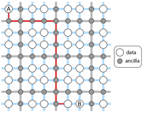
Figure 3: A $2D$ lattice of qubits, where half of the qubits are “data”, containing information, and half are “ancillas”, facilitating quantum routing. The logical qubit, $A$, is first teleported next to $B$ by employing the ESTP along the red trajectory; subsequently, a local two-site gate is applied to entangle the pair. Reversing the ESTP sends qubit $A$ back to its original location. The run time is constrained by (1).

5.2 Routing in two-dimensional arrays

Our bound (1) also establishes that current quantum “routing” protocols utilizing teleportation are optimal, as we now explain. Numerous quantum tasks require operations applied to well separated qubits (e.g., several widely known quantum algorithms Shor (1997); Grover (1996) and simulating dynamics with all-to-all interactions). However, many experimental quantum devices that realize arrays of qubits have only limited connectivity and often use immobile qubits (with the notable exception of trapped-ion devices).

The saturating protocol for (1) suggests that a quantum information processor with arbitrarily nonlocal connectivity can be efficiently built out of spatially localized (i.e., immobile) qubits using distributed quantum computing Beals et al. (2013). Essentially, one implements a two-site gate between arbitrarily distant qubits $A$ and $B$ via quantum routing Herbert (2018); Devulapalli et al. (2022), in which the state of qubit $A$ is teleported to an ancillary site adjacent qubit $B$, the two-body interaction is applied, and the state of the ancilla is then teleported back to the original location of qubit $A$. For example, see Fig. 3: One can use roughly half of the qubits in a $2D$ lattice as ancilla registers to teleport logical qubits across the lattice’s ancillary backbone for fast implementation of nonlocal gates. This entire process is optimized by using, e.g., the ESTP of Sec. 2.2 with $M$ measurement regions to decrease the time $T$ required.

5.3 Bell pair distillation

A simple Clifford protocol for preparing a well-separated Bell pair (2) follows from the entanglement-swapping teleportation protocol (ESTP) of Sec. 2.2. For Bell pair distillation, compared to Fig. 1, we remove qubit $A^{\,}_{1}$ along with all qubits to the left. The final Bell pair is recovered on sites $B^{\,}_{1}$ and $N=A^{\,}_{M+1}$ using one fewer measurement region compared to the ESTP depicted in Fig. 1. All other aspects of the protocol are the same.

Starting from the product state $\lvert\mathbf{0}\rangle$, we apply Bell encoding channels $\mathcal{B}$ to the $C$ and $D$ sites in each of the $M+1$ regions labelled $s=1,2,\dots,M+1$. We then use $T-2$ layers of SWAP gates—as for the ESTP—to move each Bell qubit $C^{\,}_{s}$ to site $B^{\,}_{s}$ and each Bell qubit $D^{\,}_{s}$ to site $A^{\,}_{s+1}$ with $A^{\,}_{M+2}=N$ the final site. We then perform Bell decoding $\mathcal{B}^{\dagger}$ on neighboring $A^{\,}_{s}$ and $B^{\,}_{s}$ qubits for $2\leq s\leq M+1$. For the case depicted in Fig. 1, there is only one measurement region (the first orange-shaded region of the ESTP is always excluded for Bell pair distillation). We then measure $Z^{\vphantom{*}}$ on both the $A^{\,}_{s}$ and $B^{\,}_{s}$ qubits, which determines the error-correction channel $\mathcal{R}$ to apply to site $N$ according to Tab. 1.

The default assignment recovers the Bell state (2) on qubits $B^{\,}_{1}$ and $N=A^{\,}_{M+2}$. Importantly, $m^{\,}_{A}$ and $m^{\,}_{B}$ always correspond to $Z^{\vphantom{*}}$ and $X^{\vphantom{*}}$ errors, respectively. However, we can independently choose whether to assign the $+1$ or $-1$ value to an error for each $m^{\,}_{A}$ and $m^{\,}_{B}$. The four different assignments of $\pm$ values in Tab. 1 to the QEC channel $\mathcal{R}$ corresponds to the four different Bell states.

This Bell-pair-producing modification of the ESTP is a Clifford protocol that distills a Bell state of two qubits separated by a distance $L$ given by

$$L^{\vphantom{\dagger}}_{\rm Bell}\,\leq\,2\,\left(M+1\right)\left(T-1\right)+1\,,~{}~{}$$ (83)

for $T-2$ layers of SWAP gates, two layers of CNOT gates (for Bell encoding and decoding), and $M$ measurement regions. The overall $+1$ compared to the circuit depicted in Fig. 1 comes from including two extra SWAP gates on the far left and right in parallel with the CNOTs in the Bell decoding layer (prior to the measurements). Replacing the $Z^{\vphantom{*}}$ measurements with Bell-basis measurements gives a task distance $L^{\vphantom{\dagger}}_{\rm Bell}\,<\,2\,\left(M+1\right)\,T$.

While similar protocols are certainly known in the literature, we note that (i) the protocol above allows for arbitrary tradeoffs between $M$ and $T$ and (ii) the fact that the task distance (83) saturates (1) establishes that more efficient protocols do not exist.

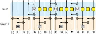
Figure 4: A protocol for generating the GHZ state (84) is depicted diagrammatically for a $1D$ chain of $N=16$ qubits with $T=4$ and $M=3$. The protocol creates and grows local GHZ states on each of the four-site patches shaded in orange. The blue-shaded portion of the protocol “patches” the local GHZ states into a single GHZ state using measurements (pointer dials), classical communication (the dashed line), and error correction (yellow boxes).

5.4 Preparing GHZ states

In Sec. 4.3 we extended the bound (1) to the preparation of GHZ states (3). We now discuss an optimal $1D$ protocol that prepares the GHZ state on $N$ qubits starting from the product state $\lvert\mathbf{0}\rangle$ (on all physical and Stinespring qubits). While aspects of this protocol are well known to the literature, the fact that this protocol saturates (1) implies (i) that more efficient protocols do not exist and (ii) that the bound (1) is optimal with respect to the preparation of GHZ states Greenberger et al. (1989, 2007); Meignant et al. (2019); Piroli et al. (2021).

As a reminder, the GHZ state is given by

$$\lvert\text{GHZ}\rangle\,\equiv\,\frac{1}{\sqrt{2}}\left(\lvert\boldsymbol{0}\rangle+\lvert\boldsymbol{1}\rangle\right)\,,~{}~{}$$ (84)

and a protocol that prepares this state in $1D$ is depicted in Fig. 4 for $N=16$, $M=3$, $T=4$. This protocol involves two distinct stages: the “growth” and “patch” stages, distinguished by orange and blue shading in Fig. 4.

The $1D$ protocol follows from Fig. 4: For a given $M\geq 0$ and $T\geq 3$, the $N$-qubit chain is divided into $M+1$ regions of size $\ell=2(T-1)$. We apply Bell encoding $\mathcal{B}$ to form a local GHZ state of the central two qubits in each region. We then apply $T-3$ layers of CNOT gates to grow these local GHZ states by two qubits per layer.

We then patch the local GHZ states together. We first apply a CNOT gate between each pair of regions, and then measure $Z^{\vphantom{*}}$ on the target qubit and reset its state to $\lvert 0\rangle$. If the measurement outcome was 1, we apply $X^{\vphantom{*}}$ to all other qubits in the same local patch as the measured state; otherwise, we do nothing. Finally, applying the same CNOT gate applied prior to measurement reincorporates the measured qubit into the GHZ state, which now contains all $N=L+1=\left(M+1\right)\,\ell$ qubits.

This $1D$ GHZ-preparation protocol with circuit depth $T$ and $M=\mathcal{M}$ single-qubit measurements satisfies

$$L^{\vphantom{\dagger}}_{\rm GHZ}\,\sim\,N\,=\,2\,\left(M+1\right)\left(T-1\right)\,,~{}~{}$$ (85)

which saturates (1) with $M^{\,}_{0}=2$ and $T^{\,}_{0}=-1$.

In $D>1$, analogous protocols saturate (1), though a slight modification to the “patch” stage is required. A protocol in $D>1$ with circuit depth $T$ and $M=\mathcal{M}$ single-qubit measurements satisfies

$$L^{D}_{\rm GHZ}\,\sim\,N\,=\,\mathsf{O}\left(M\times\left(2\,T\right)^{D}\right)\,,~{}~{}$$ (86)

and further details of the protocol—including the extension to $D>1$—appear in the SM sup .

Most importantly, the fact that (85) and (86) saturate the bound (1) implies that not only that the protocol depicted in Fig. 4 optimal, but the bound (1) itself is optimal with respect to the preparation of GHZ states.

5.5 Preparing W states

We now present a protocol for preparing W states (5) on a $1D$ chain of $N$ qubits prepared in the state $\lvert\mathbf{0}\rangle$ Piroli et al. (2021); Cruz et al. (2019). The protocol is illustrated in Fig. 5, and other technical details appear in the SM sup . As a reminder, the W state for the $N$ qubits in the set $V$ is given by

$$\lvert W\rangle\,=\,\frac{1}{\sqrt{N}}\,\sum\limits_{v\in V}\,\lvert 1\rangle^{\vphantom{\prime}}_{v}\otimes\lvert\mathbf{0}\rangle^{\vphantom{\prime}}_{V\setminus\{v\}}\,,~{}~{}$$ (87)

which is an equal-weight superposition over all configurations with a single qubit in the state $\lvert 1\rangle$ and all others in the state $\lvert 0\rangle$. Equivalently, the W state (87) is the $k=0$ quantum Fourier transform Coppersmith (2002) of the state $\lvert 1\rangle\otimes\lvert\mathbf{0}\rangle$.

In contrast to the other protocols discussed thus far, the protocol that prepares the W state (87), depicted in Fig. 5, does not saturate the corresponding bound (62), except in the $M=0$ limit where $T=\mathsf{O}\left(N\right)$. However, this protocol can be implemented in depth $T=\mathsf{O}\left(\log N\right)$, compared to the $T=\mathsf{O}\left(N\right)$ protocols described in Coppersmith (2002); Piroli et al. (2021).

The standard unitary ($M=0$) protocols for preparing the W state (87) are similar to the measurement-free protocols that prepare the GHZ state (84) Coppersmith (2002); Piroli et al. (2021). One first prepares the state $\lvert 1000\dots\rangle$ with a single flipped spin (or excitation) on the leftmost site; one then uses $\mathsf{O}\left(N\right)$ SWAP gates to move this excitation to the right, applying local single-site rotation gates (which do not count toward $T$) so that a fraction of the excitation is “left behind” Coppersmith (2002); Piroli et al. (2021). Unlike the GHZ state (84), there is no obvious means by which to use measurements to achieve an $\mathsf{O}\left(2M\right)$ enhancement to $v$. This is due in part to the fact that the W state (87) is not a stabilizer state. We also note that the protocol described in Piroli et al. (2021) replaces these $T$ SWAP gates with $T$ copies of the ESTP using ancilla qubits, so that $M,T=\mathsf{O}\left(N\right)$; however, this is far more costly than the protocol we now describe.

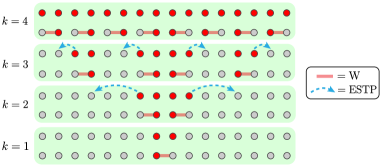
Figure 5: A protocol that generates the W state on $N=2^{n}$ sites is depicted for a $1D$ chain of $N=16$ qubits ($n=4$). The gray circles denote qubits still in the initial $\lvert 0\rangle$ state; the red circles denote the set of qubits $A$ that participate in the W state of $2^{k}$ qubits in step $k$ of the protocol. Measurements are only used to expedite the equal spacing of participating qubits in each stage via the ESTP of Sec. 2.2.

The workhorse of this W-state-preparation protocol is the following non-Clifford two-qubit gate of Cruz et al. (2019):

where the circuit above acts from left to right as

$$\operatorname{W}^{\vphantom{\dagger}}_{i,j}\,=\,\text{CNOT}\left(j\to i\right)\,\text{CH}\left(i\to j\right)\,,~{}~{}$$ (88)

meaning that $\operatorname{W}^{\,}_{i,j}$ first applies a Hadamard gate $H^{\,}_{j}=(X^{\vphantom{*}}_{j}+Z^{\vphantom{*}}_{j})/\sqrt{2}$ to qubit $j$ if qubit $i$ is in the state $\lvert 1\rangle$ (and does nothing otherwise), and then applies $X^{\vphantom{*}}_{i}$ to qubit $i$ if qubit $j$ is in the state $\lvert 1\rangle$ (and does nothing otherwise).

The non-Clifford gate $\operatorname{W}^{\,}_{i,j}$ (LABEL:eq:W_gate) can be used to double the size of an existing W state. Suppose an $\ell$-qubit subset $A\subset V$ of the physical qubits participate in a W state, while the $\ell$-qubit subset $B\subset V$ realizes the state $\lvert\mathbf{0}\rangle$. For every qubit $a\in A$ we identify a partner $b(a)\in B$ (in Fig. 5, these qubits are neighbors). We then have that

$$\lvert W\rangle^{\vphantom{\prime}}_{A\cup B}\,=\,\prod\limits_{a\in A}\,\operatorname{W}^{\vphantom{\dagger}}_{a,b(a)}\,\lvert W\rangle^{\vphantom{\prime}}_{A}\otimes\lvert\mathbf{0}\rangle^{\vphantom{\prime}}_{B}\,,~{}~{}$$ (89)

where the $\ell$ distinct gates $\operatorname{W}^{\,}_{a,b(a)}$ map the state $\lvert W\rangle^{\,}_{A}$ on $\ell$ qubits to the state $\lvert W\rangle^{\,}_{A\cup B}$ on $2\ell$ qubits. Since all $\ell$ gates can be applied in parallel, this costs $T=2$.

The following protocol creates a W state on $N=2^{n}$ qubits arranged in a $1D$ chain, and is illustrated in Fig. 5. The qubits in the initial state $\lvert 0\rangle$ are depicted as gray circles in Fig. 5, while those incorporated into the W state (87) are depicted as red circles. The protocol involves $n$ rounds in which a two-stage subroutine—corresponding to “growth” and “teleportation”—is applied.

We first seed a two-qubit W state (87)—equivalent to one of the Bell states—on the two central qubits. This is achieved in $T=1$ using the Bell encoding channel $\mathcal{B}$ followed by $X^{\vphantom{*}}$ on either qubit, and no teleportation is required. In each of the steps $1<k<n$, we first double the size of the W state as in (89) by applying $\operatorname{W}^{\,}_{a,b}$ gates, where $a$ runs over the incorporated qubits (the red circles in Fig. 5) and the corresponding unincorporated qubit $b(a)$ is the outward neighbor to $a$. We then teleport the newly incorporated $b(a)$ qubits by $L^{\,}_{k}=2^{n-k}-1$ sites (indicated by blue arrows in Fig. 5), which concludes the $k$th round. In the final round $k=n$, all $N/2$ remaining qubits are incorporated into the W state, without the need for teleportation, concluding the protocol.

As with the other protocols presented in this paper, this W-state-preparation protocol allows tradeoffs between $M$ and $T$. However, measurements are only helpful in expediting the “teleportation” step of each round $k$. In the absence of measurements ($M=0$), teleportation in round $k$ is achieved using $T=2^{n-k}-1$ layers of SWAP gates, so that the total circuit depth is

$$T^{\vphantom{\dagger}}_{\rm max}\,=\,\frac{1}{2}N+\log_{2}N-1\,<\,N,~{}~{}$$ (90)

which saturates the measurement-free bound $T\lesssim N$ Lieb and Robinson (1972).

Alternatively, we can use the ESTP to teleport the newly incorporated qubits in the steps $2\leq k\leq n-2$. Full details appear in the SM sup . Essentially, in round $k$ there are $2^{k-1}$ newly incorporated qubits, which we can teleport a distance $L^{\,}_{k}=2^{n-k}-1$ in parallel. In each of the $2^{k-1}$ teleportation regions, the ESTP first applies a SWAP gate to the qubit being teleported and its less central neighbor, and then generates $2^{n-k-1}-1$ Bell pairs per region. In each round $k$, only the outermost two regions utilize new measurement locations, and thus the $k$th round with minimum depth involves $2^{n}-2^{k}$ total measurement outcomes, and $2^{n-k}-2$ new measurement regions. Note that we eschew the Bell-decoding channels of the ESTP as depicted in Fig. 1, replacing the measurements of $Z^{\vphantom{*}}_{A}$ and $Z^{\vphantom{*}}_{B}$ with $M^{\,}_{k}$ Bell measurements of $X^{\vphantom{*}}_{A}X^{\vphantom{*}}_{B}$ and $Z^{\vphantom{*}}_{A}Z^{\vphantom{*}}_{B}$, respectively. The error-correction channel $\mathcal{R}$ is still determined according to Tab. 1.

Each round $k\in[2,n-2]$ requires circuit depth $T^{\,}_{k}=3$ and measurements in $2^{n-k}-2$ new regions, with $2^{n}-2^{k}$ new outcomes. The first round has $T=1$, the last round has $T=2$, and the penultimate round has $T=3$ (where teleportation is replaced by SWAP gates); these three rounds do not require measurements. The total resource costs are given by

$$T^{\vphantom{\dagger}}_{\rm min}\, =\,3\,\log_{2}N-3$$ (91a)

$$M^{\vphantom{\dagger}}_{\rm max}\, =\,N/2-2\,\log_{2}N+2\,,~{}~{}$$ (91b)

so that the depth scales as $T=\mathsf{O}\left(\log N\right)$ while the number of independent regions obeys $M\lesssim N$. Additionally, the number of measurement outcomes utilized scales as $\mathcal{M}=\mathsf{O}\left(N\,\log N\right)$. While using the ESTP to expedite the teleportation steps leads to a significant speed up compared to the $M=0$ case (90), this protocol does not saturate the bound (62) for $M>0$.

Importantly, although it does not saturate (62) or (63), this protocol generates the W state (5) faster than all protocols known to the literature—i.e., $T\sim\log_{2}N$ instead of $T\sim N$ Coppersmith (2002); Piroli et al. (2021). Most likely, it is the protocol above—rather than the bound (62) or (63)—that is suboptimal with respect to preparing $\lvert W\rangle$ (5). We also suspect that $T\gtrsim\log_{2}N$ is a generic bound on the measurement-based preparation of $W$, Dicke, and other nonstabilizer states with long-range correlations. However, we leave the proof of these conjectures to future work Hong et al. (2023b).

5.6 Locality of measurements

The unitary measurement formalism Friedman et al. (2022) detailed in Sec. 3 is a mathematical consequence of the Stinespring Dilation Theorem Stinespring (1955). Physically, the measurement channel (32) is unitary because—in an idealized limit—it describes the evolution of both the system and apparatus under measurement Barberena and Friedman (2023); Friedman et al. (2022); Everett (1956). A key advantage of this unitary representation is the ability to evolve operators in the Heisenberg picture in the presence of generic quantum channels, leading to the main bound (1).

However, the locality of measurements is also quite transparent applying the Stinespring formalism to the evolution of states. For example, consider the Bell state (2), where one qubit is sent to Alice and the other to Bob, who each measure $Z^{\vphantom{*}}$ on their respective qubits. The dilated state prior to measurement is

$$\lvert\text{Bell}\rangle\, =\,\frac{1}{\sqrt{2}}\left(\lvert 00\rangle+\lvert 11\rangle\right)^{\,}_{AB}\otimes\lvert 00\rangle^{\,}_{ab}$$

$$=\,\frac{1}{\sqrt{2}}\left(\lvert 00,00\rangle+\lvert 11,00\rangle\right)\,,~{}~{}$$ (92)

where, in the second line, the qubits correspond to $\lvert AB,ab\rangle$ with $A$ and $B$ the physical qubits for Alice and Bob and $a$ and $b$ the corresponding Stinespring qubits (i.e., the states of the two measurement apparati).

The measurement channels (32) corresponding to the two $Z^{\vphantom{*}}$ measurements are given by $\mathsf{V}^{\,}_{A}=\text{CNOT}(A\to a)$ and $\mathsf{V}^{\,}_{B}=\text{CNOT}(B\to b)$. Following the measurements, the state of the physical and Stinespring qubits is

$$\lvert\Psi\rangle\, =\,\mathsf{V}^{\vphantom{\dagger}}_{A}\,\mathsf{V}^{\vphantom{\dagger}}_{B}\,\lvert\text{Bell}\rangle\,=\,\mathsf{V}^{\vphantom{\dagger}}_{B}\,\mathsf{V}^{\vphantom{\dagger}}_{A}\,\lvert\text{Bell}\rangle$$

$$=\,\frac{1}{\sqrt{2}}\left(\lvert 00,00\rangle+\lvert 11,11\rangle\right)\,,~{}~{}$$ (93)

i.e., each measurement merely entangles the state of the apparatus with the state of the physical qubit.

More importantly, this entangling interaction is local. Note that the $a$ and $A$ qubits must be close by for the measurement to occur (and likewise for the $b$ and $B$ qubits). Additionally, the order of measurements is unimportant, and neither measurement ($A$/$B$) affects the state of the other physical qubit ($B$/$A$), suggesting that measurements alone cannot send quantum information nor generate entanglement or correlations.

In fact, this conclusion is even more generic. Provided that the state of the physical qubits is represented in the eigenbasis of the operator to be measured, measurements have no effect whatsoever on the physical state. For example, suppose that Alice intends to measure $Z^{\vphantom{*}}$ while Bob intends to measure $X^{\vphantom{*}}$. In the $Z^{\vphantom{*}}_{A}\otimes X^{\vphantom{*}}_{B}$ basis, the same Bell state (92) takes the form

$$\lvert\text{Bell}\rangle\, =\,\frac{1}{2}\left(\lvert 00\rangle+\lvert 01\rangle+\lvert 10\rangle-\lvert 11\rangle\right)\otimes\lvert 00\rangle\,,~{}~{}$$ (94)

and because we have written $\lvert\text{Bell}\rangle$ (94) in the measurement basis, the measurement channels again act as CNOT gates. After the two measurements, we find

$$\lvert\Psi\rangle =\mathsf{V}^{\vphantom{\dagger}}_{A}\,\mathsf{V}^{\vphantom{\dagger}}_{B}\,\lvert\text{Bell}\rangle\,=\,\mathsf{V}^{\vphantom{\dagger}}_{B}\,\mathsf{V}^{\vphantom{\dagger}}_{A}\,\lvert\text{Bell}\rangle$$

$$=\frac{1}{2}\left(\lvert 00,00\rangle+\lvert 01,01\rangle+\lvert 10,10\rangle-\lvert 11,11\rangle\right)\,,$$ (95)

so that the physical state is completely unaltered by the measurements. This is generic to any set of commuting measurement channels applied to qubits, when the state is expressed in the measurement basis.

The unitary representation of measurements Friedman et al. (2022); Barberena and Friedman (2023) applied to states elucidates why there is nothing paradoxical about measuring Bell states Einstein et al. (1935); Bell (1964). Additionally, this picture shows that information is not transferred—nor can entanglement or correlations be generated—using measurements of entangled states alone.

However, as demonstrated by numerous protocols detailed herein, the inclusion of a classical communication channel indicating the outcomes of measurements, followed by a quantum error-correction channel conditioned on those outcomes, is not only compatible with—but can expedite by a factor of $M+1$—the transfer of quantum information and generation of entanglement and/or correlations, provided that the bound (1) is obeyed.

5.7 Summary of results

We prove an emergent, finite speed of quantum information in the presence of arbitrary local quantum dynamics, projective measurements, instantaneous classical communications, and outcome-dependent operations captured by the main bound (1). That bound extends to arbitrary, finite-dimensional degrees of freedom assigned to any graph $G$ in any spatial dimension $D$. The bound holds for both time-dependent Hamiltonians and quantum circuits acting on connected regions of bounded size, which may depend arbitrarily on prior measurement outcomes. The bound extends the Lieb-Robinson Theorem Lieb and Robinson (1972) to generic quantum dynamics with measurements, feedback, and instantaneous classical communication for the first time.

The bound also captures generic local quantum channels (e.g., weak measurements). Additionally, we derive the bound (74) for the generation of $Q$ Bell pairs and the teleportation of $Q$ logical qubits, and recover numerous bound on the preparation of various classes of correlated states in Sec. 4.3. In this sense, our bounds constrain generic quantum tasks, which either generate or manipulate quantum information, entanglement, or correlations using local operations, which may depend on the outcomes of measurements, whose communication is instantaneous.

Prior to this work—and the development of the Stinespring formalism (see also Friedman et al. (2022); Barberena and Friedman (2023))—such a feat was not thought possible. Not only was the mathematical machinery required to evolve operators out of reach, but conventional wisdom held that measurements destroy any emergent notion of spatial locality. Our bound (1) proves that this is not the case by establishing a finite, $\mathsf{O}\left(M\right)$ enhancement to the measurement-free Lieb-Robinson velocity $v$ Lieb and Robinson (1972); Foss-Feig et al. (2015); Chen and Lucas (2019); Kuwahara and Saito (2020); Tran et al. (2020); Eisert and Gross (2009); Schuch et al. (2011); Kuwahara and Saito (2021); Yin and Lucas (2022) provided that the outcomes of measurements in $M$ local regions are known and utilized.

Our bound (1) constrains the most efficient quantum protocols (which feature measurements) for transferring quantum information and generating long-range entanglement and/or correlations, while highlighting the essential role of error-correcting feedback in performing generic useful quantum tasks. Applications of (1) include quantum error correction, measurement-based quantum computation, quantum routing, and the preparation of generic long-range-entangled many-body states of interest to condensed matter and atomic physics. We provide explicit, optimal protocols for numerous such tasks, establishing optimality of the bound (1) in these contexts.

As measurements both increase the speed of information and the additional qubits and resources necessary for active error-correction, our bound may elucidate fundamental limits on the operation of a large-scale quantum information processor built out of physical qubits.

As with the Lieb-Robinson Theorem Lieb and Robinson (1972) itself, there is no telling what new applications of the bound (1) the future may hold in store. In the near term, we expect that applications of (1) and the Stinespring formalism Friedman et al. (2022) will provide deep insight through more specialized consideration of various quantum tasks Hong et al. (2023a, b). Additionally, (1) provides for a more general classification of phases of matter, as it proves that states with short- and long-range entanglement cannot be connected by protocols $\mathcal{W}$ for which the combined resources $M\times T$ are finite, generalizing the concept of finite-depth circuits. More broadly, we hope that our results will lead to more efficient strategies for preparing useful resource states, achieving useful tasks, and optimizing compiling on near-term quantum devices.

See pages 1 of supplement.pdf

See pages 2 of supplement.pdf

See pages 3 of supplement.pdf

See pages 4 of supplement.pdf

See pages 5 of supplement.pdf

See pages 6 of supplement.pdf

See pages 7 of supplement.pdf

See pages 8 of supplement.pdf

See pages 9 of supplement.pdf

See pages 10 of supplement.pdf

See pages 11 of supplement.pdf

See pages 12 of supplement.pdf

See pages 13 of supplement.pdf

See pages 14 of supplement.pdf

See pages 15 of supplement.pdf

See pages 16 of supplement.pdf

See pages 17 of supplement.pdf

See pages 18 of supplement.pdf

See pages 19 of supplement.pdf

See pages 20 of supplement.pdf

See pages 21 of supplement.pdf

See pages 22 of supplement.pdf

See pages 23 of supplement.pdf

See pages 24 of supplement.pdf

See pages 25 of supplement.pdf

See pages 26 of supplement.pdf

See pages 27 of supplement.pdf

See pages 28 of supplement.pdf

See pages 29 of supplement.pdf

See pages 30 of supplement.pdf

See pages 31 of supplement.pdf

See pages 32 of supplement.pdf

See pages 33 of supplement.pdf

See pages 34 of supplement.pdf

See pages 35 of supplement.pdf

See pages 36 of supplement.pdf

See pages 37 of supplement.pdf

See pages 38 of supplement.pdf

See pages 39 of supplement.pdf

See pages 40 of supplement.pdf

See pages 41 of supplement.pdf

See pages 42 of supplement.pdf

See pages 43 of supplement.pdf

See pages 44 of supplement.pdf

See pages 45 of supplement.pdf

See pages 46 of supplement.pdf

See pages 47 of supplement.pdf

See pages 48 of supplement.pdf

See pages 49 of supplement.pdf

See pages 50 of supplement.pdf

See pages 51 of supplement.pdf

See pages 52 of supplement.pdf

See pages 53 of supplement.pdf

See pages 54 of supplement.pdf

See pages 55 of supplement.pdf

See pages 56 of supplement.pdf

See pages 57 of supplement.pdf

See pages 58 of supplement.pdf

See pages 59 of supplement.pdf

See pages 60 of supplement.pdf

See pages 61 of supplement.pdf

See pages 62 of supplement.pdf

See pages 63 of supplement.pdf

References

- Lieb and Robinson (1972) Elliott H. Lieb and Derek W. Robinson, “The finite group velocity of quantum spin systems,” Comm. Math. Phys. 28, 251–257 (1972).
- Foss-Feig et al. (2015) Michael Foss-Feig, Zhe-Xuan Gong, Charles W. Clark, and Alexey V. Gorshkov, “Nearly linear light cones in long-range interacting quantum systems,” Phys. Rev. Lett. 114, 157201 (2015).
- Chen and Lucas (2019) Chi-Fang Chen and Andrew Lucas, “Finite speed of quantum scrambling with long range interactions,” Phys. Rev. Lett. 123, 250605 (2019).
- Kuwahara and Saito (2020) Tomotaka Kuwahara and Keiji Saito, “Strictly linear light cones in long-range interacting systems of arbitrary dimensions,” Phys. Rev. X 10, 031010 (2020).
- Tran et al. (2020) Minh C. Tran, Chi-Fang Chen, Adam Ehrenberg, Andrew Y. Guo, Abhinav Deshpande, Yifan Hong, Zhe-Xuan Gong, Alexey V. Gorshkov, and Andrew Lucas, “Hierarchy of linear light cones with long-range interactions,” Phys. Rev. X 10, 031009 (2020).
- Eisert and Gross (2009) J. Eisert and D. Gross, “Supersonic quantum communication,” Phys. Rev. Lett. 102, 240501 (2009).
- Schuch et al. (2011) Norbert Schuch, Sarah K. Harrison, Tobias J. Osborne, and Jens Eisert, “Information propagation for interacting-particle systems,” Phys. Rev. A 84, 032309 (2011).
- Kuwahara and Saito (2021) Tomotaka Kuwahara and Keiji Saito, “Lieb-Robinson bound and almost-linear light cone in interacting boson systems,” Phys. Rev. Lett. 127, 070403 (2021).
- Yin and Lucas (2022) Chao Yin and Andrew Lucas, “Finite speed of quantum information in models of interacting bosons at finite density,” Phys. Rev. X 12 (2022).
- Jünemann et al. (2013) J. Jünemann, A. Cadarso, D. Pérez-García, A. Bermudez, and J. J. García-Ripoll, “Lieb-Robinson bounds for spin-boson lattice models and trapped ions,” Phys. Rev. Lett. 111, 230404 (2013).
- Poulin (2010) David Poulin, “Lieb-Robinson bound and locality for general Markovian quantum dynamics,” Phys. Rev. Lett. 104, 190401 (2010).
- Lucas (2020) Andrew Lucas, “Nonperturbative dynamics of the operator size distribution in the Sachdev–Ye–Kitaev model,” J. Math. Phys. 61, 081901 (2020).
- Einstein et al. (1935) A. Einstein, B. Podolsky, and N. Rosen, “Can quantum-mechanical description of physical reality be considered complete?” Phys. Rev. 47, 777–780 (1935).
- Li et al. (2021) Yaodong Li, Xiao Chen, Andreas W. W. Ludwig, and Matthew P. A. Fisher, “Conformal invariance and quantum nonlocality in critical hybrid circuits,” Phys. Rev. B 104, 104305 (2021).
- Ippoliti et al. (2021) Matteo Ippoliti, Michael J. Gullans, Sarang Gopalakrishnan, David A. Huse, and Vedika Khemani, “Entanglement phase transitions in measurement-only dynamics,” Phys. Rev. X 11, 011030 (2021).
- Bao et al. (2021) Yimu Bao, Maxwell Block, and Ehud Altman, “Finite-time teleportation phase transition in random quantum circuits,” arXiv (2021).
- Piroli et al. (2021) Lorenzo Piroli, Georgios Styliaris, and J. Ignacio Cirac, “Quantum circuits assisted by local operations and classical communication: Transformations and phases of matter,” Phys. Rev. Lett. 127, 220503 (2021).
- Verresen et al. (2021) Ruben Verresen, Nathanan Tantivasadakarn, and Ashvin Vishwanath, “Efficiently preparing Schrödinger’s cat, fractons and non-Abelian topological order in quantum devices,” arXiv (2021).
- Tantivasadakarn et al. (2021) Nathanan Tantivasadakarn, Ryan Thorngren, Ashvin Vishwanath, and Ruben Verresen, “Long-range entanglement from measuring symmetry-protected topological phases,” arXiv (2021).
- Bell (1964) J. S. Bell, “On the Einstein-Podolsky-Rosen paradox,” Physics Physique Fizika 1, 195–200 (1964).
- Briegel et al. (1998) H.-J. Briegel, W. Dür, J. I. Cirac, and P. Zoller, “Quantum repeaters: The role of imperfect local operations in quantum communication,” Phys. Rev. Lett. 81, 5932–5935 (1998).
- Herbert (2018) Steven Herbert, “On the depth overhead incurred when running quantum algorithms on near-term quantum computers with limited qubit connectivity,” arXiv (2018).
- Devulapalli et al. (2022) Dhruv Devulapalli, Eddie Schoute, Aniruddha Bapat, Andrew M. Childs, and Alexey V. Gorshkov, “Quantum routing with teleportation,” arXiv (2022).
- Bennett et al. (1993) Charles H. Bennett, Gilles Brassard, Claude Crépeau, Richard Jozsa, Asher Peres, and William K. Wootters, “Teleporting an unknown quantum state via dual classical and Einstein-Podolsky-Rosen channels,” Phys. Rev. Lett. 70, 1895–1899 (1993).
- Chung et al. (2009) Thomas Chung, Stephen D. Bartlett, and Andrew C. Doherty, “Characterizing measurement-based quantum gates in quantum many-body systems using correlation functions,” Can. J. Phys. 87, 219–224 (2009).
- (26) See Supplemental Material at [url] for additional details .
- Stinespring (1955) W. Forrest Stinespring, “Positive functions on -algebras,” Proc. Amer. Math. Soc. 6, 211 (1955).
- Friedman et al. (2022) Aaron J. Friedman, Oliver Hart, and Rahul Nandkishore, “Measurement-induced phases of matter require adaptive dynamics,” arXiv (2022), arXiv:2210.07256 [quant-ph] .
- Barberena and Friedman (2023) Diego Barberena and Aaron J. Friedman, “Theory of projective quantum measurements,” arXiv , to appear (2023).
- Hong et al. (2023a) Yifan Hong, David T. Stephen, and Aaron J. Friedman, “Clifford teleportation implies symmetry-protected topological order,” arXiv , to appear (2023a).
- Else et al. (2012) Dominic V. Else, Ilai Schwarz, Stephen D. Bartlett, and Andrew C. Doherty, “Symmetry-protected phases for measurement-based quantum computation,” Phys. Rev. Lett. 108 (2012).
- Jozsa (2005) Richard Jozsa, “An introduction to measurement-based quantum computation,” arXiv (2005).
- Greenberger et al. (1989) Daniel M Greenberger, Michael A Horne, and Anton Zeilinger, “Going beyond Bell’s theorem,” in Bell’s theorem, quantum theory and conceptions of the universe (Springer, 1989) pp. 69–72.
- Greenberger et al. (2007) Daniel M. Greenberger, Michael A. Horne, and Anton Zeilinger, “Going beyond Bell’s theorem,” arXiv (2007).
- Meignant et al. (2019) Clément Meignant, Damian Markham, and Frédéric Grosshans, “Distributing graph states over arbitrary quantum networks,” Phys. Rev. A 100, 052333 (2019).
- Sachdev (2000) Subir Sachdev, Quantum Phase Transitions (Cambridge University Press, 2000).
- Francesco et al. (2012) Philippe Francesco, Pierre Mathieu, and David Sénéchal, Conformal field theory (Springer Science & Business Media, 2012).
- Lu et al. (2022) Tsung-Cheng Lu, Leonardo A. Lessa, Isaac H. Kim, and Timothy H. Hsieh, “Measurement as a shortcut to long-range entangled quantum matter,” PRX Quantum 3, 040337 (2022).
- Dicke (1954) R. H. Dicke, “Coherence in spontaneous radiation processes,” Phys. Rev. 93, 99–110 (1954).
- Dür et al. (2000) W. Dür, G. Vidal, and J. I. Cirac, “Three qubits can be entangled in two inequivalent ways,” Phys. Rev. A 62, 062314 (2000).
- Ma et al. (2011) Jian Ma, Xiaoguang Wang, C.P. Sun, and Franco Nori, “Quantum spin squeezing,” Phys. Reports 509, 89–165 (2011).
- Kitagawa and Ueda (1993) Masahiro Kitagawa and Masahito Ueda, “Squeezed spin states,” Phys. Rev. A 47, 5138–5143 (1993).
- Wineland et al. (1992) D. J. Wineland, J. J. Bollinger, W. M. Itano, F. L. Moore, and D. J. Heinzen, “Spin squeezing and reduced quantum noise in spectroscopy,” Phys. Rev. A 46, R6797–R6800 (1992).
- Peres (1985) Asher Peres, “Reversible logic and quantum computers,” Phys. Rev. A 32, 3266–3276 (1985).
- Shor (1995) Peter W. Shor, “Scheme for reducing decoherence in quantum computer memory,” Phys. Rev. A 52, R2493–R2496 (1995).
- Steane (1996a) Andrew Steane, “Multiple-particle interference and quantum error correction,” Proc. Roy. Soc. London. A: MPES 452, 2551–2577 (1996a).
- Steane (1996b) A. M. Steane, “Error correcting codes in quantum theory,” Phys. Rev. Lett. 77, 793–797 (1996b).
- DiVincenzo and Shor (1996) David P. DiVincenzo and Peter W. Shor, “Fault-tolerant error correction with efficient quantum codes,” Phys. Rev. Lett. 77, 3260–3263 (1996).
- Gottesman (1998) Daniel Gottesman, “Theory of fault-tolerant quantum computation,” Phys. Rev. A 57, 127–137 (1998).
- Hong et al. (2023b) Yifan Hong, Chao Yin, Aaron Friedman, and Andrew Lucas, “Untitled work on the w state,” arXiv , to appear (2023b).
- Nielsen and Chuang (2010) Michael A. Nielsen and Isaac L. Chuang, Quantum Computation and Quantum Information: 10th Anniversary Edition (Cambridge University Press, 2010).
- Barenco et al. (1995) Adriano Barenco, Charles H. Bennett, Richard Cleve, David P. DiVincenzo, Norman Margolus, Peter Shor, Tycho Sleator, John A. Smolin, and Harald Weinfurter, “Elementary gates for quantum computation,” Phys. Rev. A 52, 3457–3467 (1995).
- Choi (1975) Man-Duen Choi, “Completely positive linear maps on complex matrices,” Linear Algebra and its Applications 10, 285–290 (1975).
- Everett (1956) Hugh Everett, III, The Theory of the Universal Wave Function, Ph.D. thesis, Princeton U. (1956).
- Hong et al. (2022) Yifan Hong, Jeremy T. Young, Adam M. Kaufman, and Andrew Lucas, “Quantum error correction in a time-dependent transverse-field ising model,” Phys. Rev. A 106 (2022).
- Gottesman and Chuang (1999) Daniel Gottesman and Isaac L. Chuang, “Demonstrating the viability of universal quantum computation using teleportation and single-qubit operations,” Nature 402, 390–393 (1999).
- Hoyer and Spalek (2005) Peter Hoyer and Robert Spalek, “Quantum fan-out is powerful,” Theory of Computing 1, 81–103 (2005).
- Browne et al. (2010) Dan Browne, Elham Kashefi, and Simon Perdrix, “Computational depth complexity of measurement-based quantum computation,” in Theory of Quantum Computation, Communication, and Cryptography, Vol. 6519 (Springer Berlin Heidelberg, 2010) pp. 35–46.
- Bao et al. (2020) Yimu Bao, Soonwon Choi, and Ehud Altman, “Theory of the phase transition in random unitary circuits with measurements,” Phys. Rev. B 101, 104301 (2020).
- Hamming (1950) R. W. Hamming, “Error-detecting and error-correcting codes,” Bell Sys. Tech. J. 29, 147–160 (1950).
- Calderbank and Shor (1996) A. R. Calderbank and Peter W. Shor, “Good quantum error-correcting codes exist,” Phys. Rev. A 54, 1098–1105 (1996).
- Bravyi and Kitaev (1998) S. B. Bravyi and A. Yu. Kitaev, “Quantum codes on a lattice with boundary,” arXiv (1998), 10.48550/ARXIV.QUANT-PH/9811052.
- Dennis et al. (2002) Eric Dennis, Alexei Kitaev, Andrew Landahl, and John Preskill, “Topological quantum memory,” J. Math. Phys. 43, 4452–4505 (2002).
- Kitaev (2003) A.Yu. Kitaev, “Fault-tolerant quantum computation by anyons,” Annals Phys. 303, 2–30 (2003).
- Kitaev (2006) Alexei Kitaev, “Anyons in an exactly solved model and beyond,” Ann. Phys. 321, 2–111 (2006).
- Wilson (1974) Kenneth G. Wilson, “Confinement of quarks,” Phys. Rev. D 10, 2445–2459 (1974).
- Shor (1997) P. W. Shor, “Polynomial-time algorithms for prime factorization and discrete logarithms on a quantum computer,” SIAM J. Comp. 26, 1484–1509 (1997).
- Grover (1996) Lov K. Grover, “A fast quantum mechanical algorithm for database search,” arXiv (1996), 10.48550/arxiv.QUANT-PH/9605043, 9605043 .
- Beals et al. (2013) Robert Beals, Stephen Brierley, Oliver Gray, Aram W. Harrow, Samuel Kutin, Noah Linden, Dan Shepherd, and Mark Stather, “Efficient distributed quantum computing,” Proc. Roy. Soc. A: MPES 469, 20120686 (2013).
- Cruz et al. (2019) Diogo Cruz, Romain Fournier, Fabien Gremion, Alix Jeannerot, Kenichi Komagata, Tara Tosic, Jarla Thiesbrummel, Chun Lam Chan, Nicolas Macris, Marc-André Dupertuis, and Clément Javerzac-Galy, “Efficient quantum algorithms for GHZ and W states, and implementation on the IBM quantum computer,” Adv. Quant. Tech. 2 (2019).
- Coppersmith (2002) D. Coppersmith, “An approximate Fourier transform useful in quantum factoring,” arXiv (2002).