A Temperature Trend for Clouds and Hazes in Exoplanets Atmospheres

Abstract

The transmission spectra of exoplanet atmospheres observed with the Hubble Space Telescope (HST) in the near-infrared range (1.1-1.65$\mu$m) frequently show evidence for some combination of clouds and hazes. Identification of systematic trends in exoplanet clouds and hazes is potentially important for understanding atmospheric composition and temperature structure. Here we report on the analysis of spectral modulation using a large, uniformly processed sample of HST/WFC3 transit spectra from 62 exoplanets. The spectral retrieval includes the capability to detect and represent atmospheres in which the composition departs from thermochemical equilibrium. By using this unique catalog and measuring the dampening of spectral modulations compared to strictly clear atmospheres, we identify two populations. One is completely cloud/haze free spanning a wide temperature range, while the other population, identified as “Partial cloud/hazes”, follows a trend from mostly cloudy/hazy around 500 K to mostly clear at $\sim$1500 K. We also find that a partially transparent aerosol component is frequently present and that it is typically vertically distributed throughout the atmospheric column. Our findings also suggest that while clouds and hazes are common in exoplanet atmospheres, the majority of planets have some level of detectable spectral modulation. Additionally, the empirical trend that clouds and hazes are minimized at 1460.86K${}^{+316}_{-405}$ revealed in our catalog has predictive utility for modelling the performance of large-scale transiting exoplanets survey, such as planned with the Ariel mission. This trend can also be used for making a probability-based forecast of spectral modulation for a given source in the context of future JWST observations. Future observations including the optical and/or a broader spectral coverage may be useful to further quantify the trend reported here.

1 Introduction

NASA’s Hubble Space Telescope (HST) has been used to observe exoplanet transits at wavelengths ranging from the ultraviolet (UV) to the visible to the near infrared (NIR) as long as 2.4 $\mu$m (Charbonneau et al., 2002; Vidal-Madjar et al., 2003; Swain et al., 2021; Deming et al., 2013). However, the majority of HST transiting-exoplanet spectroscopic observations have been conducted with the Wide Field Camera 3 (WFC3) instrument using the spatial-scan mode and the G141 grism covering wavelengths from 1.1 $\mu$m to 1.6 $\mu$m. Comparative planetology studies based on these observations show that the spectral modulation seen in the transmission spectra indicate atmospheres can vary from obscured to clear (Sing et al., 2016). The nature of the obscuring aerosols, which we will term “clouds and hazes” is an area of active investigation, and possible candidates range from various condensed species to photochemically produced hazes. The cloudy and hazy atmospheres are associated with a weaker absorption feature in the NIR portion of the transmission spectrum of the planet or a featureless spectra (Knutson et al., 2014a, b; Kreidberg et al., 2014). Although some of the low spectral amplitudes could also be associated with low water abundances, as has been pointed out by previous works (Barstow et al., 2017; Pinhas et al., 2019; Welbanks et al., 2019). While in the optical spectra, clouds/hazes can cause Rayleigh scattering–like opacity seen in several planets (Pont et al., 2008, 2013; McCullough et al., 2014; Sing et al., 2016; Estrela et al., 2021). These clouds are generally attributed to atmospheric condensates of salt, silicate, and metal vapors (Morley et al., 2012; Zhang, 2020; Gao et al., 2020), or to photochemically produced hazes due to energy input or energetic particle bombardment (Lavvas & Koskinen, 2017; Lavvas et al., 2019; Gao et al., 2020; Lavvas & Arfaux, 2021). Clouds and hazes can have a critical role in planetary atmospheres. They can affect the amount of light reflected by the atmosphere of the planet, which determines the Bond albedo and consequently the equilibrium temperature of the planet (Cahoy et al., 2010). They can also control the thermal structure, chemistry, and dynamics in the atmosphere (Tomasko & West, 2010; Müller-Wodarg et al., 2014).

A wide range of potential cloud compositions may be plausible due to the significant possibility of condensate materials (Zhang, 2020) and because of exoplanet properties, the potential for migration, and differences in formation/evolutionary scenarios. Particularly, cloud composition depends on the temperature of the atmosphere. Various scenarios using temperature dependence to infer cloud composition have been modeled (Burrows & Sharp, 1999; Morley et al., 2013; Parmentier et al., 2016). Some molecules will condense at high temperatures (e.g., TiO/VO, Al, and Ca), while others prefer moderate temperatures (e.g., Fe, Mg, Si, Cr, and Mn) or lower temperatures (e.g., K and Na) (Gao et al., 2021). Observations of exoplanet atmospheres illustrate this diversity. Many species, such as TiO/VO and metals, have been suggested to be present in ultrahot Jupiters (Ben-Yami et al., 2020; Cabot et al., 2020; Changeat et al., 2022), while smaller and cooler planets (sub-Neptunes and super-Earths) also have indicated the presence of high-altitude aerosols in their atmospheres (Ehrenreich et al., 2014; Wakeford et al., 2017; Kreidberg et al., 2020). Other planets have shown very steep optical slope in their spectra (Alderson et al., 2020; Estrela et al., 2021; Chen et al., 2021) due to scattering in the atmosphere, which could be explained by sulphide clouds (MnS, ZnS, Na₂S) (Pinhas & Madhusudhan, 2017). High-altitude photochemical hazes could also lead to super-Rayleigh optical slope, depending on their mixing and formation rate (Ohno & Kawashima, 2020). Advances in laboratory experiments are helping to better constrain cloud formations, and simulations for hot Jupiters’ atmospheres and even smaller planets’ atmospheres have shown photochemical haze production (Hörst et al., 2018; Fleury et al., 2019, 2020; Yu et al., 2021).

In addition to understanding cloud formation, the overall level of “cloudiness” in exoplanet atmospheres is a topic of great interest for planning exoplanet observations because of the potential for strong clouds to dampen spectral features and thus compromise the study of atmospheric composition (Kreidberg et al., 2014). A robust method of predicting the likelihood and impact of clouds and hazes in the detection of exoplanet atmospheres is of great value for planning observations. For example, the Ariel mission (Tinetti et al., 2018; Zellem et al., 2019) will conduct a transit spectroscopy survey of hundreds of exoplanets, and the ability to estimate cloud properties could be an important factor in planning the mission observations. Also, the detectability of molecular features on smaller planets with the James Webb Space Telescope (JWST) could be significantly compromised due to the presence of clouds/hazes (Fauchez et al., 2019). Several studies have used HST/WFC3-G141 transmission spectra to conduct statistical analysis using the amplitude of the water feature to identify planets affected by the presence of clouds/hazes. Based on the HST/WFC3-G141 catalog of Tsiaras et al. (2018), Iyer et al. (2016); Fu et al. (2017); Fisher & Heng (2018); Gao et al. (2020) have found that most planets had their amplitude diminished by aerosols when compared to a clear atmosphere. (Wakeford et al., 2019) show that 30% of the time the amplitude of the water spectral feature is find to be below 0.5Hs which deviates from a cloud-free scenario. An analysis by Stevenson (2016) suggest that there is a threshold for cloudiness level at a surface gravity of 2.8 dex. More recently, Dymont et al. (2021) have searched for correlations between cloudiness metrics and other physical parameters such as temperature using sample sizes of 23 planets. However, as noted by Dymont et al. (2021), the lack of a uniform data reduction was a less-than-ideal aspect of the sample they studied.

Given the importance of clouds and hazes for establishing planet properties and their impact on characterization using the transit spectroscopy method, additional investigation into the properties of exoplanet clouds and hazes is a priority. Rapid progress in exoplanet observations is leading to the ability to improve sample size with respect to previous works. Here, we report on an analysis of clouds and hazes using the largest uniformly processed exoplanet transmission spectra catalog available in Roudier et al. (2021).

2 Methodology

Detection of clouds and hazes is typically done through measuring the degree of spectral modulation (Sing et al., 2016), which can then be compared to estimates of the theoretical possible values (Iyer et al., 2016; Gao et al., 2020) or plotted against various physical parameters to search for correlations (Stevenson, 2016; Fu et al., 2017; Fisher & Heng, 2018; Gao et al., 2020; Dymont et al., 2021). Here, we perform this analysis using the catalog from Roudier et al. (2021) that consists of 62 planets observed with the WFC3 instrument onboard the HST using the G141 infrared (IR) grism (1.1–1.6 $\mu$m) spatial scan observations. Compared with previous works, this exoplanet catalog has three important advantages for the study of clouds. First, this catalog is the largest uniformly processed catalog of HST transmission spectra that has been published. In this case, the data have all been processed though the same pipeline, and they have all been analyzed with the same spectral retrieval code. A uniformly processed catalog is particularly important when performing comparative planetology because differences in planetary spectra can be attributed to differences in astrophysics rather than analysis methods. Second, this catalog is based on the EXoplanet CALIbration and Bayesian Unified Retrieval (EXCALIBUR) pipeline (Swain et al., 2021; Roudier et al., 2021; Estrela et al., 2021; Huber-Feely et al., 2022), which processes HST/WFC3-G141 data at the full spectral resolution of the instrument. Using the full G141 spectral resolution avoids the potential reduction in spectral feature amplitude that can be caused by additional spectral averaging. Third, the CERBERUS spectral retrieval code, used for modeling the transmission spectra in this catalog, is capable of modeling atmospheres assuming both thermal equilibrium chemistry (TEC) and disequilibrium chemistry (DisEQ). The majority of previous works interpreted planet populations observed with the HST/WFC3 instrument as being consistent only with bulk TEC conditions, while atmospheres can undergo DisEQ due to photochemistry, which can be associated with a water-depleted spectrum. The DisEQ atmosphere assumed by Roudier et al. (2021) does not fully exclude water but includes water as a subdominant feature and brings the possibility of other dominant signatures such as CH₄, C₂H₂, HCN, and CO₂. Roudier et al. (2021) identifies a third category of planets that could not be determined, based on the model selection criteria, to be either DisEQ or TEC. We term this category “Indeterminate” and divide this group into those that have spectral modulation greater than 1H_s and those that do not.

To estimate the amplitude of the spectral modulation in the transmission spectra, we take the difference between the Maximum and Minimum of the CERBERUS preferred model (henceforth referred to as CMM) in the NIR range between 1.15–1.6 $\mu$m (see Fig. 2). This method is based on the approach of Iyer et al. (2016) and has the advantage of naturally debiasing the impact of individual spectral channel values on estimates of spectral modulation. In the case of TEC models, the CMM will measure the strength of the water feature, while for the DisEQ planets it will measure the strength of the other possible dominant features (CH₄, C₂H₂, HCN, and CO₂). To facilitate the analysis, we convert the CMM to units of planetary scale height H_s:

$$H_{s}=\frac{k_{B}T_{eq}}{\mu g},$$ (1)

where $k_{B}$ is the Boltzmann constant, $\mu$ is the mean molecular weight of an atmosphere in solar composition ($\mu$ = 2.3 amu), $g$ is the surface gravity, and $T_{eq}$ is the calculated equilibrium temperature.

Next, we build an index of the spectral modulation that represents a fraction of the potential modulation a planet achieves. This index is obtained by dividing the difference between the CMM of the spectral modulation of the regular retrieved model (CMM_CRB) by the CMM of the cloud/haze free model (CMM_FREE) of each individual target:

$$Spec_{\rm index}=\frac{\rm CMM_{\rm CRB}}{\rm CMM_{\rm FREE}}$$ (2)

This index varies from 0 to 1, where 0 accounts for cloudy/hazy and 1 represents a clear atmosphere. The cloud/haze free model is obtained by setting the haze/clouds parameters to zero (see Fig. 1 for comparison between the retrieved model and the cloud/haze-free model).

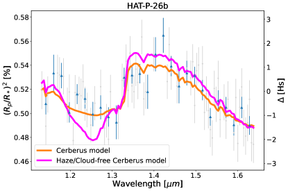
Figure 1: Comparison between the retrieved Cerberus model for the target HAT-P-26b and the model without clouds and hazes used to obtain the spectral modulation index.

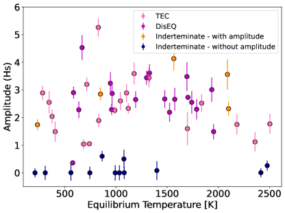
Figure 2: Amplitude of the spectral modulation in TEC (light pink), DisEQ (magenta), and Indeterminate (orange) targets in terms of scale height.

2.1 Clouds and Hazes

We also analyze the properties of the hazes and clouds obtained with the atmospheric retrieval CERBERUS. To derive information on the haze layer, CERBERUS uses a parametrization of Jupiter’s haze profiles (Zhang et al., 2015) constructed by taking the median of the haze latitude number density. The following free parameters characterize the haze properties and are retrieved by CERBERUS:

• HScale: Multiplicative scale factor (log10) of the haze optical depth (common to all pressure layers). In CERBERUS, the optical depth per length element $\tau$/dl [m^-1] is given by:

  $$\rm\frac{\tau_{cerb}}{dl}=\rm HScale\times\rho_{cerb}\times\sigma_{cerb}$$ (3)

  where $\rm\rho_{cerb}$ and $\rm\sigma_{cerb}$ are the haze density profile and cross section in CERBERUS, respectively.

• HLoc: The maximum density location of the haze cloud in log pressure (bars)

• HThick: Multiplicative factor (log10) of the width of the density haze profile

We illustrate in Fig. 4 how these parameters can vary for exoplanets. The aerosol density profile has a log-pressure maximum density location (HLoc) that is allowed to linearly translate vertically in the atmosphere. A multiplicative factor (HThick) is introduced to compress or stretch the vertical extent of the initial profile. Another multiplicative factor (HScale) is used to scale the haze optical depth for each pressure layer. In addition, the modeled atmosphere includes a bottom opaque cloud-top pressure (CTP) in a log unit of bars.

3 Results

The estimated amplitude of the spectral modulation of the TEC, DisEQ, and Indeterminate targets is shown in Fig. 2. The Indeterminate targets are classified into two groups: those with minimal to no spectral modulation and those with detected modulation $>=$1H_s. Targets in these groups are indecisive between TEC and DisEQ because the evidence of the model is not strong enough, and the model cannot decide between TEC or DisEQ to explain any modulation there. Fig. 2 shows that our sample is very diverse in terms of equilibrium temperature. The distribution of the modulation varies from planets that have large modulation and are potentially cloud/haze free to those with minimal spectral modulation that could be in a completely aerosol-dominated scenarios or have high molecular weight atmospheres. See appendix for values of the spectral amplitude presented in Fig. 2.

The planets’ range of cloudiness/haziness level is also well-illustrated in Fig. 3 through the spectral modulation index (see description in Section 2). We identify two groups in Fig. 3. One group is cloud/haze-free (blue region) with spectral modulation indexes above 0.9 that is distributed across different temperatures. Within this group, there are a few “Indeterminate” targets that have indexes greater than 1.3 due to steep slopes towards short wavelengths. We exclude these particular targets because their slopes could be associated to Rayleigh scattering by clouds/hazes or atmospheric escape. The second group has some level of cloudiness/haziness and we identified them as “Partial clouds/hazes” region (in grey). If we exclude the completely cloud/haze-dominated (blue targets in Fig. 2) and the cloud/haze-free targets, the “Partial clouds/hazes” targets show a rise in the spectral modulation index between 500–1500 K, indicating that we expect more clear atmospheres for planets with temperatures between $\sim$1200–1500 K. This trend is consistent with laboratory studies (Yu et al., 2021) that show that in the temperature range of 500–800 K, hazes can be removed more efficiently by direct deposition to the surface or deep atmosphere. Also, the trend seen from 500–1500 K is also in agreement with the cloudy-to-clear trend from 500-1000K seen in previous observational studies Crossfield & Kreidberg (2017); Libby-Roberts et al. (2020); Guilluy et al. (2021) for warm Neptunes. Planets with higher temperatures ($>$ 1700K) seem to indicate more cloudy/hazy atmospheres although we lack sufficient data to make firm conclusions. However, it is possible that heat transport is very inefficient above 1600 K, which would allow the nightside to cool and clouds to advect to the dayside (Parmentier et al., 2021). The temperature trend in the spectral modulation is well fitted using a second-order polynomial. The fit gives the relationship:

$$y=-2.9e-7^{+7.1e-8}_{-7.1e-8}x^{2}+8.4e-4^{+2e-4}_{-2e-4}x+1.4e-2^{+0.13}_{-0.13}.$$ (4)

If we fit a 4th order polynomial to the data (dashed blue line in Fig. 3), we see a trend raising towards reduced cloud/hazy atmospheres at low temperatures planets ($<$ 270K) in the Habitable Zone (HZ), K2-18b and LHS 1140b, where liquid water can exist and condense. This trend is also explained by laboratory studies (Yu et al., 2021), which has shown that high surface energy hazes can be formed in these planets and they are efficiently removed by cloud droplets formed through water condensation. However, any conclusions can’t be made due the lack of targets at lower temperatures. In addition, the 2nd order polynomial is still the best fit for the “Partial clouds/hazes” population (although the 4th order is not excluded), as shown by the Bayesian information criterion (BIC). The BIC for each fit is calculated by:

$${\rm BIC}=\chi^{2}+k\ln(n)$$ (5)

where $k$ is the number of free parameters, represented by the polynomial order plus 1, and n is the number of data points. The best model is the one with the lowest BIC, which is the quadratic model, as shown in Table 1. We also estimated the delta BIC with respect to the best model, and found a value of 0.6 for the 4-th model which provides weak evidence that the quadratic model is better. On the other hand, the linear model has a delta BIC greater than 10, which represents strong evidence that the quadratic model is better.

Model	BIC	$\Delta$BIC	$\Delta$BIC rules of thumb
Linear	190	70	evidence against the linear model is strong
2nd order	120	0	best model
3rd order	123	3	evidence against the 3rd order polynomial is moderate
4th order	121	1	weak evidence that best model is better

Table 1: Bayesian Inference Criteria (BIC) for each model fitted to the ‘Partial clouds/hazes” population.

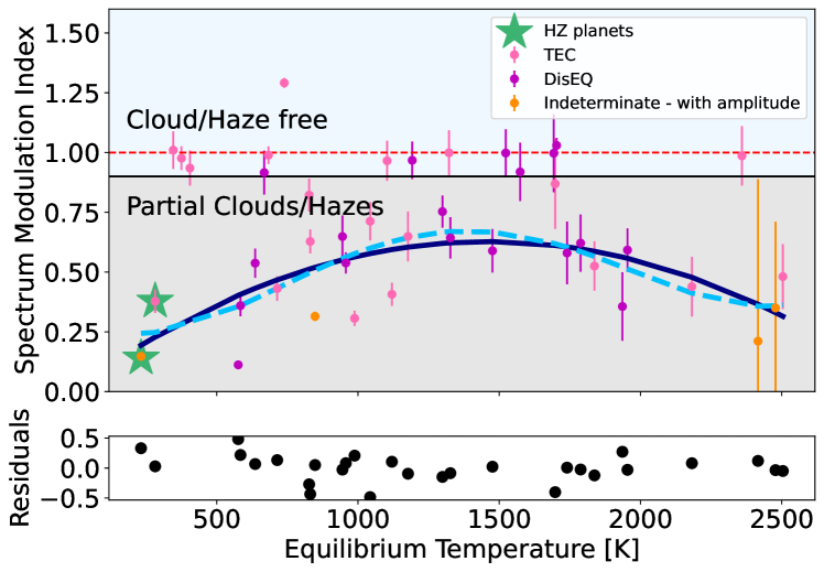
Figure 3: [Top] Spectral modulation index of the TEC (light pink), DisEQ (magenta) and Indeterminate (orange) targets from the Roudier et al. (2021) catalog gives the cloudiness level of each target. The solid blue line shows the best-fit for the “Partial clouds/hazes” targets (within grey region), a second-order polynomial to the data that can be used as a forecast of spectral modulation to future missions. The dashed blue line shows a 4th order polynomial that highlights an increase in reduced hazy/cloudy atmospheres for the lower temperatures planets that are in the habitable zone. The blue shaded region indicates the zone of the targets with cloud/haze-free atmospheres. [Bottom] Residual of the spectral modulation index subtracted from the model.

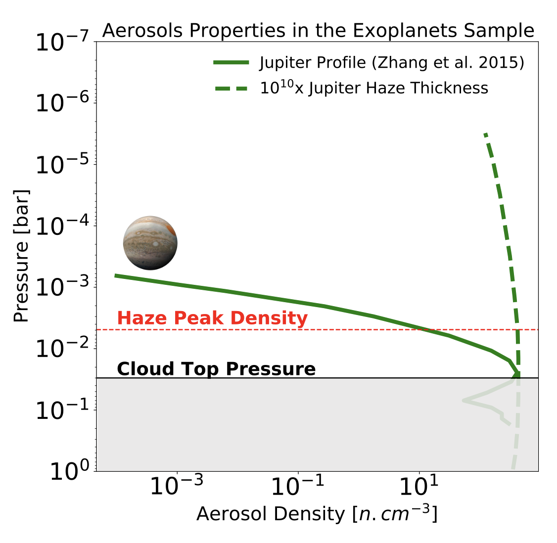
Figure 4: Comparison between the Jupiter’s haze profile and the scaled haze model obtained with the averaged aerosol properties found in the exoplanet sample. The thickness of Jupiter’s haze layer is shown by a solid line and the median thickness found for the exoplanet catalog in this study is indicated by a dashed line. For the exoplanet model, we also illustrate the location of the haze peak density (in terms of pressure) in red and the cloud top pressure (CTP), indicated by a solid line. Any atmospheric content below the CTP (within the grey region) would be muted.

Considering that future missions would largely benefit from a forecast of spectral modulation for planning observations, we note that the second order polynomial trend can be used to make a spectral modulation forecast. Including the forecast for the temperature dependence for spectral modulation has the potential to increase the fidelity of planning observations with JWST and Ariel, and based on the results of this study, we would anticipate that plenty of targets would likely show modulation in their spectra.

3.1 Aerosol Properties

Another key result that comes from the analysis of the Roudier et al. (2021) exoplanet catalog of TEC and DisEQ targets relies on the aerosol properties. To infer the aerosol properties, we take the best solution obtained with the CERBERUS atmospheric retrieval code by parametrizing the Jupiter aerosol layer (see Section 2). We find that this sample of exoplanets has a much more extended haze layer than Jupiter, and it is widely distributed throughout the atmosphere. The CTP is very similar in both TEC and DisEQ targets, showing pressures of $\sim$0.05 bars, which means that any atmospheric column below that pressure is blocked by the cloud layer and not sampled by transmission spectroscopy. These results are summarized in Table 2 and illustrated in Fig. 4, where the thickness of the haze layer, the location of the peak density, and the multiplicative factor of the haze opacity (with respect to Jupiter’s opacity) are shown.

We caution that our haze model parameters are a parametric scaling of Jupiter’s haze properties and thus do not capture the detailed microphysics of haze formation in these much hotter exoplanets. Our modeling suggests that haze in exoplanet atmospheres is typically distributed widely throughout the atmospheric column, similar to what was found for HD 209458b by Lavvas & Koskinen (2017) based on a microphysics model for haze formation. Similarly, our modeling suggests that the presence of a bottom cloud is detectable and influences the interpretation of WFC3/G141 observations. However, detailed physical conclusions about the vertical distribution of the haze and bottom cloud properties will need to be addressed with models that appropriately represent the chemistry and physics of these atmospheres—and we identify this as an area for further investigation.

Aerosol and Cloud Properties of the TEC and DisEQ Exoplanets in the Sample
	TEC	DisEQ	Indeterminate
HScale	0.008	0.0006	0.70
HLoc	0.005 bars	0.006 bars	0.003 bars
HThick	5.8 $\times$ 109	5.5 $\times$ 109	4.7 $\times$ 1010
CTP	0.03 bars	0.06 bars	0.002 bars

Table 2: Median values of the aerosol properties (HScale, HLoc, HThick) and the cloud top pressure (CTP) of the TEC and DisEQ population obtained with the atmospheric retrieval CERBERUS.

4 Discussion

4.1 Cloudy/Hazy-to-Clear Atmospheres

One of the key results from our analysis is that planets can take on a wide range of values from clear to cloudy atmospheres, but they are frequently somewhere in between, implying that the majority of the planets has some content of clouds and/or hazes. This result is consistent with previous work by Sing et al. (2016) that shows that planets can have cloudy and/or hazy or clear atmospheres. Although some of the observed low spectral amplitudes Sing et al. (2016) have been shown to be caused by low water abundances rather than by clouds/hazes exclusively (Barstow et al., 2017; Pinhas et al., 2019; Welbanks et al., 2019). Our work also supports the claim that clouds/haze can indeed mute spectral features, as previously discussed by Iyer et al. (2016). However, in the majority of cases, the atmospheres still have detectable spectral features that are sufficient for detailed study, such as whether the atmosphere is TEC or DisEQ.

4.2 Extended Aerosol Layer in Exoplanets

We find that the planets in our catalog have a population of aerosol particles that are typically widely vertical through the exoplanet atmosphere ($\sim$4 orders of magnitude in pressure). This wide distribution of particles raises questions about whether they could be condensates, as the T-P profile could vary considerably over this pressure range. Another possible explanation could be photochemical haze particles, as they have been shown to be distributed throughout the atmospheric column of the planet HD 189733b extending from 10² bar to millibars (Lavvas & Koskinen, 2017). However, the composition of the clouds is not explored in detail in this work because condensation of materials is strongly dependent on the temperature, and our atmospheric temperature is obtained with a 1D atmospheric retrieval, which in some cases can lead to biased values of the temperature of the atmosphere (Welbanks & Madhusudhan, 2022). Therefore, further investigation is needed to determine the nature of the aerosol particles.

4.3 Forecasting Spectral Modulation

Using the spectral amplitudes seen in our catalog, we estimate a spectrum modulation index that varies from 0 to 1, where 0 would be a cloudy atmosphere with no spectral amplitude and 1 would be a cloud-free atmosphere. We found a quadratic polynomial trend in the spectrum modulation index of the targets within the partial clouds/hazes region that can be used for forecasting cloudiness/haziness for a given source that could be potentially observed by current or future missions. By taking the derivative of this equation, we get that the minimum clouds/haze occurs at 1460.86${}^{+316}_{-405}$ K. The empirically determined trend is useful for forecasting the level of spectral modulation that will be detected in large-surveys, such as the one planned with the Ariel mission. Our findings suggest that additional time in the form of repeated visits should be considered for observations of lower temperature planets to increase the signal to noise of the transit spectrum to compensate for the reduction in spectral modulation caused by clouds and hazes. A larger sample such as the one anticipated by Ariel will certainly be useful for improving this type of empirical constraint on cloud/haze impacts on spectral modulation.

Step	Dependence Chain	Reference Used
Make Spectra	4 pixels spectra averaging	Tsiaras et al. (2018)
Model Spectra	TEC only model	Fu et al. (2017)
	H2O as the dominant opacity source
Estimate Modulation	Max/Min of best fit model at 1.3-1.65$\mu$m	Fu et al. (2017)
Step	Dependence Chain in this work	Reference Used
Make Spectra	No Averaging	Roudier et al. (2021)
Model Spectra	TEC and DisEQ models	Roudier et al. (2021)
	Many molecular species
Estimate Modulation	Max/Min of probable model at 1.1 and 1.6$\mu$m	Roudier et al. (2021)

Table 3: Summary of the key differences between the methods used in previous works in the literature and those used in this work.

4.4 Differences Between EXCALIBUR and Previous Works

In addition to conducting an analysis using a large, uniformly observed and processed catalog of transit spectra, there are two key aspects of our analysis. The first is that the transit spectra in this catalog are processed at the full spectral resolution of the HST/WFC3 instrument. The key advantage here is that it minimizes the potential for reducing spectral modulation by low-pass filtering. A previous sample analyzed by Fu et al. (2017) did not use a full resolution of the spectrum as EXCALIBUR does. Their sample was based on the data reduction by Tsiaras et al. (2018) that used a 4-pixel spectral averaging while our sample does not average spectral bins. Similarly, Edwards et al. (2022) applied the methods of Tsiaras et al. (2018) and Fu et al. (2017) to a larger sample and find qualitatively consistent results to Fu et al. (2017). Spectral averaging has the clear potential to decrease spectral modulation. The second key aspect is that the spectral retrieval analysis for the EXCALIBUR catalog can model both TEC and DisEQ atmospheric composition scenarios, including atmospheres that show spectral modulation due to water vapor. Thus, unlike some previous work (Fu et al., 2017; Fisher & Heng, 2018; Gao et al., 2020; Dymont et al., 2021; Edwards et al., 2022), our approach can measure and model spectral modulation independent of whether a water signature is present in the spectrum. Assuming only water to be the possible opacity in the spectrum has the potential to force a water-model fit to a water-depleted atmosphere, which could result in lower spectral modulation. This constitutes a substantial difference from the approach taken previously and is a point that needs to be borne in mind when comparing our results to previous work.

Another difference between our catalog and previous work relies on the estimation of the spectral modulation. Here, we take the difference between the maximum and minimum of the most probable CERBERUS model in that interval, while Fu et al. (2017) takes the difference between the maximum and minimum of the best-fit water model. All these factors together, summarized in Table 3, could explain the difference in trend seen in the amplitude of the spectral modulation between our work and that of the previous sample by Fu et al. (2017), with the average amplitude found by EXCALIBUR being higher.

However, similar to Dymont et al. (2021), planets in our catalog that are below 1000 K can vary widely in terms of cloudiness around the overall trend. Also, our work seems to quantitatively agree with the quadratic polynomial trend seen in Yu et al. (2021) that shows an increase in clear atmospheres from 500 K to 800 K. The inclusion of visible wavelengths would have the potential to reveal a better picture of the dominance of haze and clouds in the atmospheres, as has been explored by previous works (Heng, 2016; Pinhas et al., 2019). Therefore, future catalogs may benefit from including the spectral modulation from observations taken by the Space Telescope Imaging Spectrograph (STIS) on the HST. However, the merge of HST/STIS and HST/WFC3 can be challenging since there are multiple factors that could compromise the interpretation: (1) the average planet/star ratios measured with HST/STIS can be different from than that obtained with HST/WFC3, and this difference could be associated with intrinsic properties of the atmosphere, or due to different instrument systematics or stellar activity (Estrela et al., 2021); (2) effects from unocculted star spots that could produce slopes in the optical transmission spectrum (Rackham et al., 2017).

5 Conclusions

This work performs comparative planetology of a large, uniformly observed and processed catalog of transit spectra that were obtained at the full spectral resolution of the HST/WFC3 instrument. Our method is consistent for a large range of planet properties, and the sample is larger than those used in previous works. Another differentiating aspect of this work when compared with previous studies is that the spectral catalog used here is modeled with both TEC and DisEQ atmospheric composition scenarios. This implies that the spectral modulation in exoplanet spectra is modeled assuming not only H₂O but also other dominant spectral features due to disequilibrium chemistry. The amplitude of the spectral modulation in our catalog reveals that exoplanet atmospheres vary from cloudy to clear, with most of the planets typically lying in between. This suggests that transiting exoplanet atmospheres contain detectable spectral features that are partially muted. From the analysis of the haze properties, we find that haze layer is partially transparent and widely extended throughout the atmospheric column.

In addition, we estimated a spectral modulation index that quantifies the cloudiness/haziness in each target. We observe that there are two groups of planets, one is completely cloud/haze free spanning a wide temperature range. The other group, denominated “Partial cloud/haze”, follows a trend from cloudy/hazy to clear within 500–1500 K in the spectral modulation, with the least cloudy atmospheres lying at 1460.86K${}^{+316}_{-405}$. This trend is consistent with previous observational samples and laboratory studies from Yu et al. (2021) that indicate efficient haze removal in that temperature range. We find that a quadratic polynomial is the best fit for the trend seen in the spectral modulation indexes. However, a 4th order polynomial trend shows a rise of reduced hazy/cloudy atmospheres for planets with temperatures lower than 270K, including those in the HZ. At these temperatures, water can condense and hazes can be removed by wet deposition (Yu et al., 2021). The empirical quadratic polynomial trend can be used for predicting cloudiness/haziness for modeling large-scale surveys. This is particularly beneficial for forecasting potential targets that could have their atmospheres observed by JWST or future missions devoted to the the observation of exoplanet atmospheres, such as Ariel. A potentially more robust improvement in the estimation of the spectral modulation index could be achieved by including the measurements on the optical wavelengths from HST/STIS in future catalogs. HST/STIS can give information on scattering due to haze and clouds, and would provide a more definitive picture of the range of cloudiness in exoplanet atmospheres.

Appendix A Supplementary Material

Spectral Modulation Amplitude – TEC
Planet	Teq [K]	Amplitude [Hs]
GJ 3470b	683	1.04 $\pm$ 0.18
HAT-P-11b	831	1.89 $\pm$ 0.24
HAT-P-26b	1043	2.60 $\pm$ 0.33
HAT-P-32b	1837	2.52 $\pm$ 0.32
K2-18b	282	2.89 $\pm$ 0.25
K2-3c	375	2.04 $\pm$ 0,25
WASP-107b	739	1.05 $\pm$ 0.10
WASP-12b	2504	1.77 $\pm$ 0.36
WASP-17b	1698	1.60 $\pm$ 0.60
WASP-39b	1120	2.33 $\pm$ 0.19
WASP-6b	1103	2.89 $\pm$ 0.33
WASP-69b	988	2.26 $\pm$ 0.14
WASP-76b	2182	1.75 $\pm$ 0.37
WASP-80b	827	5.26 $\pm$ 0.33
XO-1b	1177	3.59 $\pm$ 0.40
HAT-P-1b	1322	3.44 $\pm$ 0.35
HD 97658b	714	3.20 $\pm$ 0.25
TRAPPIST-1b	405	1.49 $\pm$ 0.37
WASP-121b	2359	1.12 $\pm$ 0.35

Table A.1: Spectral Modulation Amplitude obtained with the Roudier et al. (2021) catalog of the TEC planets.

Spectral Modulation Amplitde – DisEQ
Planet	Teq [K]	Amplitude [Hs]
GJ 1132b	584	2.90 $\pm$ 0.22
GJ 1214b	576	0.36 $\pm$ 0.04
GJ 436b	636	2.28 $\pm$ 0.3
HAT-P-12b	957	2.29 $\pm$ 0.2
HAT-P-17b	945	3.24 $\pm$ 0.4
HAT-P-41b	1936	3.01 $\pm$ 0.44
HD 189733b	1192	2.65 $\pm$ 0.3
HD 209458b	1476	2.67 $\pm$ 0.32
KELT-11b	1703	2.73 $\pm$ 0.1
WASP-29b	962	2.87 $\pm$ 0.44
WASP-31b	1574	2.66 $\pm$ 0.41
WASP-52b	1299	3.44 $\pm$ 0.25
WASP-63b	1523	2.19 $\pm$ 0.34
WASP-74b	1788	2.30 $\pm$ 0.37
WASP-79b	1740	2.55 $\pm$ 0.41
55Cnc e	1954	1.49 $\pm$ 0.28
GJ 9827b	668	4.53 $\pm$ 0.45
XO-2b	1327	3.61 $\pm$ 0.32
HD 149026b	1693	3.48 $\pm$ 0.52
TRAPPIST-1c	346	2.55 $\pm$ 0.4

Table A.2: Spectral Modulation Amplitude obtained with the Roudier et al. (2021) catalog of the planets under DisEQ.

Spectral Modulation Amplitude – Indeterminate
Planet	Teq [K]	Amplitude [Hs]
GJ 3053b	232	1.74 $\pm$ 0.2
HAT-P-18b	848	2.85 $\pm$ 0.23
HAT-P-38b	1077	0.50 $\pm$ 0.33
HATS-7b	1080	0.00 $\pm$ 0.23
K2-24b	744	0.00 $\pm$ 0.22
K2-3d	308	0.00 $\pm$ 0.25
K2-33b	864	0.60 $\pm$ 0.19
K2-96c	559	0.00 $\pm$ 0.29
KELT-1b	2416	0.00 $\pm$ 0.16
KELT-7b	2089	3.56 $\pm$ 0.55
Kepler-16b	208	0.00 $\pm$ 0.16
WASP-101b	1565	4.13 $\pm$ 0.43
WASP-18b	2478	0.26 $\pm$ 0.18
WASP-19b	2100	2.32 $\pm$ 0.26
WASP-62b	1399	0.08 $\pm$ 0.34
WASP-67b	1033	0.00 $\pm$ 0.27

Table A.3: Spectral Modulation Amplitude obtained with the Roudier et al. (2021) catalog of the planets that could not be determined, based on model selection criteria of the the atmospheric retrieval, to be either DisEQ or TEC.

References

- Alderson et al. (2020) Alderson, L., Kirk, J., López-Morales, M., et al. 2020, MNRAS, 497, 5182, doi: 10.1093/mnras/staa2315
- Barstow et al. (2017) Barstow, J. K., Aigrain, S., Irwin, P. G. J., & Sing, D. K. 2017, ApJ, 834, 50, doi: 10.3847/1538-4357/834/1/50
- Ben-Yami et al. (2020) Ben-Yami, M., Madhusudhan, N., Cabot, S. H. C., et al. 2020, ApJ, 897, L5, doi: 10.3847/2041-8213/ab94aa
- Burrows & Sharp (1999) Burrows, A., & Sharp, C. M. 1999, ApJ, 512, 843, doi: 10.1086/306811
- Cabot et al. (2020) Cabot, S. H. C., Madhusudhan, N., Welbanks, L., Piette, A., & Gandhi, S. 2020, MNRAS, 494, 363, doi: 10.1093/mnras/staa748
- Cahoy et al. (2010) Cahoy, K. L., Marley, M. S., & Fortney, J. J. 2010, ApJ, 724, 189, doi: 10.1088/0004-637X/724/1/189
- Changeat et al. (2022) Changeat, Q., Edwards, B., Al-Refaie, A. F., et al. 2022, ApJS, 260, 3, doi: 10.3847/1538-4365/ac5cc2
- Charbonneau et al. (2002) Charbonneau, D., Brown, T. M., Noyes, R. W., & Gilliland, R. L. 2002, ApJ, 568, 377, doi: 10.1086/338770
- Chen et al. (2021) Chen, G., Pallé, E., Parviainen, H., et al. 2021, MNRAS, 500, 5420, doi: 10.1093/mnras/staa3555
- Crossfield & Kreidberg (2017) Crossfield, I. J. M., & Kreidberg, L. 2017, AJ, 154, 261, doi: 10.3847/1538-3881/aa9279
- Deming et al. (2013) Deming, D., Wilkins, A., McCullough, P., et al. 2013, ApJ, 774, 95, doi: 10.1088/0004-637X/774/2/95
- Dymont et al. (2021) Dymont, A. H., Yu, X., Ohno, K., Zhang, X., & Fortney, J. J. 2021, arXiv e-prints, arXiv:2112.06173. https://arxiv.org/abs/2112.06173
- Edwards et al. (2022) Edwards, B., Changeat, Q., Tsiaras, A., et al. 2022, arXiv e-prints, arXiv:2211.00649. https://arxiv.org/abs/2211.00649
- Ehrenreich et al. (2014) Ehrenreich, D., Bonfils, X., Lovis, C., et al. 2014, A&A, 570, A89, doi: 10.1051/0004-6361/201423809
- Estrela et al. (2021) Estrela, R., Swain, M. R., Roudier, G. M., et al. 2021, AJ, 162, 91, doi: 10.3847/1538-3881/ac0c7c
- Fauchez et al. (2019) Fauchez, T. J., Turbet, M., Villanueva, G. L., et al. 2019, ApJ, 887, 194, doi: 10.3847/1538-4357/ab5862
- Fisher & Heng (2018) Fisher, C., & Heng, K. 2018, MNRAS, 481, 4698, doi: 10.1093/mnras/sty2550
- Fleury et al. (2019) Fleury, B., Gudipati, M. S., Couturier-Tamburelli, I., & Carrasco, N. 2019, Icarus, 321, 358, doi: 10.1016/j.icarus.2018.11.030
- Fleury et al. (2020) Fleury, B., Gudipati, M. S., Henderson, B. L., & Swain, M. 2020, ApJ, 899, 147, doi: 10.3847/1538-4357/aba828
- Fu et al. (2017) Fu, G., Deming, D., Knutson, H., et al. 2017, ApJ, 847, L22, doi: 10.3847/2041-8213/aa8e40
- Gao et al. (2021) Gao, P., Wakeford, H. R., Moran, S. E., & Parmentier, V. 2021, Journal of Geophysical Research (Planets), 126, e06655, doi: 10.1029/2020JE006655
- Gao et al. (2020) Gao, P., Thorngren, D. P., Lee, E. K. H., et al. 2020, Nature Astronomy, 4, 951, doi: 10.1038/s41550-020-1114-3
- Guilluy et al. (2021) Guilluy, G., Gressier, A., Wright, S., et al. 2021, AJ, 161, 19, doi: 10.3847/1538-3881/abc3c8
- Heng (2016) Heng, K. 2016, ApJ, 826, L16, doi: 10.3847/2041-8205/826/1/L16
- Hörst et al. (2018) Hörst, S. M., He, C., Lewis, N. K., et al. 2018, Nature Astronomy, 2, 303, doi: 10.1038/s41550-018-0397-0
- Huber-Feely et al. (2022) Huber-Feely, N., Swain, M. R., Roudier, G., & Estrela, R. 2022, AJ, 163, 22, doi: 10.3847/1538-3881/ac341a
- Iyer et al. (2016) Iyer, A. R., Swain, M. R., Zellem, R. T., et al. 2016, ApJ, 823, 109, doi: 10.3847/0004-637X/823/2/109
- Knutson et al. (2014a) Knutson, H. A., Benneke, B., Deming, D., & Homeier, D. 2014a, Nature, 505, 66, doi: 10.1038/nature12887
- Knutson et al. (2014b) Knutson, H. A., Dragomir, D., Kreidberg, L., et al. 2014b, ApJ, 794, 155, doi: 10.1088/0004-637X/794/2/155
- Kreidberg et al. (2014) Kreidberg, L., Bean, J. L., Désert, J.-M., et al. 2014, Nature, 505, 69, doi: 10.1038/nature12888
- Kreidberg et al. (2020) Kreidberg, L., Mollière, P., Crossfield, I. J. M., et al. 2020, arXiv e-prints, arXiv:2006.07444. https://arxiv.org/abs/2006.07444
- Lavvas & Arfaux (2021) Lavvas, P., & Arfaux, A. 2021, MNRAS, 502, 5643, doi: 10.1093/mnras/stab456
- Lavvas & Koskinen (2017) Lavvas, P., & Koskinen, T. 2017, ApJ, 847, 32, doi: 10.3847/1538-4357/aa88ce
- Lavvas et al. (2019) Lavvas, P., Koskinen, T., Steinrueck, M. E., García Muñoz, A., & Showman, A. P. 2019, ApJ, 878, 118, doi: 10.3847/1538-4357/ab204e
- Libby-Roberts et al. (2020) Libby-Roberts, J. E., Berta-Thompson, Z. K., Désert, J.-M., et al. 2020, AJ, 159, 57, doi: 10.3847/1538-3881/ab5d36
- McCullough et al. (2014) McCullough, P. R., Crouzet, N., Deming, D., & Madhusudhan, N. 2014, ApJ, 791, 55, doi: 10.1088/0004-637X/791/1/55
- Morley et al. (2013) Morley, C. V., Fortney, J. J., Kempton, E. M. R., et al. 2013, ApJ, 775, 33, doi: 10.1088/0004-637X/775/1/33
- Morley et al. (2012) Morley, C. V., Fortney, J. J., Marley, M. S., et al. 2012, ApJ, 756, 172, doi: 10.1088/0004-637X/756/2/172
- Müller-Wodarg et al. (2014) Müller-Wodarg, I., Griffith, C. A., Lellouch, E., & Cravens, T. E. 2014, Titan: Interior, surface, atmosphere, and space environment, Vol. 14 (Cambridge University Press)
- Ohno & Kawashima (2020) Ohno, K., & Kawashima, Y. 2020, ApJ, 895, L47, doi: 10.3847/2041-8213/ab93d7
- Parmentier et al. (2016) Parmentier, V., Fortney, J. J., Showman, A. P., Morley, C., & Marley, M. S. 2016, ApJ, 828, 22, doi: 10.3847/0004-637X/828/1/22
- Parmentier et al. (2021) Parmentier, V., Showman, A. P., & Fortney, J. J. 2021, MNRAS, 501, 78, doi: 10.1093/mnras/staa3418
- Pinhas & Madhusudhan (2017) Pinhas, A., & Madhusudhan, N. 2017, MNRAS, 471, 4355, doi: 10.1093/mnras/stx1849
- Pinhas et al. (2019) Pinhas, A., Madhusudhan, N., Gandhi, S., & MacDonald, R. 2019, MNRAS, 482, 1485, doi: 10.1093/mnras/sty2544
- Pont et al. (2008) Pont, F., Knutson, H., Gilliland, R. L., Moutou, C., & Charbonneau, D. 2008, MNRAS, 385, 109, doi: 10.1111/j.1365-2966.2008.12852.x
- Pont et al. (2013) Pont, F., Sing, D. K., Gibson, N. P., et al. 2013, MNRAS, 432, 2917, doi: 10.1093/mnras/stt651
- Rackham et al. (2017) Rackham, B., Espinoza, N., Apai, D., et al. 2017, ApJ, 834, 151, doi: 10.3847/1538-4357/aa4f6c
- Roudier et al. (2021) Roudier, G. M., Swain, M. R., Gudipati, M. S., et al. 2021, AJ, 162, 37, doi: 10.3847/1538-3881/abfdad
- Sing et al. (2016) Sing, D. K., Fortney, J. J., Nikolov, N., et al. 2016, Nature, 529, 59, doi: 10.1038/nature16068
- Stevenson (2016) Stevenson, K. B. 2016, ApJ, 817, L16, doi: 10.3847/2041-8205/817/2/L16
- Swain et al. (2021) Swain, M. R., Estrela, R., Roudier, G. M., et al. 2021, AJ, 161, 213, doi: 10.3847/1538-3881/abe879
- Tinetti et al. (2018) Tinetti, G., Drossart, P., Eccleston, P., et al. 2018, Experimental Astronomy, 46, 135, doi: 10.1007/s10686-018-9598-x
- Tomasko & West (2010) Tomasko, M. G., & West, R. A. 2010, Aerosols in Titan’s Atmosphere, ed. R. H. Brown, J.-P. Lebreton, & J. H. Waite, 297, doi: 10.1007/978-1-4020-9215-2_12
- Tsiaras et al. (2018) Tsiaras, A., Waldmann, I. P., Zingales, T., et al. 2018, AJ, 155, 156, doi: 10.3847/1538-3881/aaaf75
- Vidal-Madjar et al. (2003) Vidal-Madjar, A., Lecavelier des Etangs, A., Désert, J. M., et al. 2003, Nature, 422, 143, doi: 10.1038/nature01448
- Wakeford et al. (2019) Wakeford, H. R., Wilson, T. J., Stevenson, K. B., & Lewis, N. K. 2019, Research Notes of the American Astronomical Society, 3, 7, doi: 10.3847/2515-5172/aafc63
- Wakeford et al. (2017) Wakeford, H. R., Sing, D. K., Kataria, T., et al. 2017, Science, 356, 628, doi: 10.1126/science.aah4668
- Welbanks & Madhusudhan (2022) Welbanks, L., & Madhusudhan, N. 2022, ApJ, 933, 79, doi: 10.3847/1538-4357/ac6df1
- Welbanks et al. (2019) Welbanks, L., Madhusudhan, N., Allard, N. F., et al. 2019, ApJ, 887, L20, doi: 10.3847/2041-8213/ab5a89
- Yu et al. (2021) Yu, X., He, C., Zhang, X., et al. 2021, Nature Astronomy, 5, 822, doi: 10.1038/s41550-021-01375-3
- Zellem et al. (2019) Zellem, R. T., Swain, M. R., Cowan, N. B., et al. 2019, PASP, 131, 094401, doi: 10.1088/1538-3873/ab2d54
- Zhang (2020) Zhang, X. 2020, Research in Astronomy and Astrophysics, 20, 099, doi: 10.1088/1674-4527/20/7/99
- Zhang et al. (2015) Zhang, X., West, R. A., Irwin, P. G. J., Nixon, C. A., & Yung, Y. L. 2015, Nature Communications, 6, 10231, doi: 10.1038/ncomms10231