Constraining R_V Variation Using Highly Reddened Type Ia Supernovae from the Pantheon+ Sample

Abstract

Type Ia supernovae (SNe Ia) are powerful tools for measuring the expansion history of the universe, but the impact of dust around SNe Ia remains unknown and is a critical systematic uncertainty. One way to improve our empirical description of dust is to analyse highly reddened SNe Ia ($E(B-V)>0.4$, roughly equivalent to the fitted SALT2 light-curve parameter $c>0.3$). With the recently released Pantheon+ sample, there are 57 SNe Ia that were removed because of their high colour alone (with colours up to $c=1.61$), which can provide enormous leverage on understanding line-of-sight $R_{V}$. Previous studies have claimed that $R_{V}$ decreases with redder colour, though it is unclear if this is due to limited statistics, selection effects, or an alternative explanation. To test this claim, we fit two separate colour-luminosity relationships, one for the main cosmological sample ($c<0.3$) and one for highly reddened ($c>0.3$) SNe Ia. We find the change in the colour-luminosity coefficient to be consistent with zero. Additionally, we compare the data to simulations with different colour models, and find that the data prefers a model with a flat dependence of $R_{V}$ on colour over a declining dependence. Finally, our results strongly support that line-of-sight $R_{V}$ to SNe Ia is not a single value, but forms a distribution.

1 Introduction

Type Ia supernovae (SNe Ia) were used to discover the acceleration of the universe (Riess et al., 1998; Perlmutter et al., 1999), and are now being used to make some of the most precise measurements of the equation-of-state of dark energy ($w$, e.g., Garnavich et al., 1998; Suzuki et al., 2012; Betoule et al., 2014; Scolnic et al., 2018; DES Collaboration et al., 2019; Brout et al., 2022) and the current expansion rate parameterized by the Hubble constant ($\text{H}_{0}$, e.g., Freedman et al., 2019; Riess et al., 2021). However, recent analyses have shown that one path for improvement of these measurements depends on a better understanding of the impact of dust around SNe Ia and how it relates to the scatter found in standardized SNe Ia brightnesses (Brout & Scolnic, 2021; Popovic et al., 2021a).

One way to gain leverage in characterizing the role of dust is to analyse highly-reddened SNe Ia ($E(B-V)>0.4$), where intrinsic colour variations of the SN Ia have a marginal effect compared to extragalactic dust (Phillips et al., 2013; Scolnic & Kessler, 2016). For cosmological analyses with the SN Ia light-curve fitter SALT2 (Guy et al., 2007, 2010), highly-reddened SN Ia are cut ($-0.3<c<0.3$ with $c\sim E(B-V)-0.1$, e.g., Betoule et al., 2014; Scolnic et al., 2018; Brout et al., 2022). These SNe Ia are not used in the training of the spectral model itself (Betoule et al., 2014; Taylor et al., 2021; Brout et al., 2021), but it has not been shown that they cannot be used. In this analysis, we investigate these highly-reddened SNe Ia to constrain the evolution and variability of reddening.

Dust properties are often parameterized with the total-to-selective extinction parameter, $R_{V}$. $R_{V}$ is defined as $A_{V}/(A_{B}-A_{V})$, where $A_{V}$ is the extinction in the V band ($\lambda\sim 5500~{}\text{\AA}$), and $A_{B}$ is the extinction in the B band ($\lambda\sim 4400~{}\text{\AA}$). $R_{V}$ is known to vary for different sizes and composition of dust grains. The diffuse interstellar medium of the Milky Way galaxy has an average $R_{V}$ of $\sim$3.1 (e.g., Schultz & Wiemer, 1975; De Marchi et al., 2021).

SN Ia studies typically find $R_{V}$ values lower than the Milky Way average (e.g., Jha et al., 2007; Goobar, 2008; Burns et al., 2014). These measurements are with large light-curve samples, however, with a limited colour range ($E(B-V)<0.4$). There are some $R_{V}$ measurements with spectrophotometric data (e.g., Krisciunas et al., 2006; Elias-Rosa et al., 2006; Phillips et al., 2013; Amanullah et al., 2015; Cikota et al., 2016). These also typically measure low $R_{V}$, but these are mostly from highly reddened SNe Ia, where it is easier to constrain $R_{V}$. It is uncertain whether $R_{V}$ evolves with colour or if these results are due to selection effects.

One of the largest studies of $R_{V}$ for highly-reddened objects was in Mandel et al. (2011, hereafter M11). They look at 127 SNe Ia, with 5 having $E(B-V)>0.5$. They found that SNe Ia with a lower dust extinction, $A_{V}<0.4~{}\text{mag}$, have a relationship between colour and absolute luminosity consistent with an $R_{V}\sim 2.5\text{--}2.9$, while at high extinctions ($A_{V}>1~{}\text{mag}$) low values of $R_{V}<2$ were favoured. However, this data set is from “targeted” SN Ia surveys where the observations target larger brighter galaxies, possibly biasing the data set’s colour demographics. Contrary to M11, Gonzalez-Gaitan et al. (2021) finds that $R_{V}$ grows with SN Ia colour, though with a limited colour range to $-0.3<c<0.3$. These conflicting results indicate the complexity of the relationship between $R_{V}$ and SN Ia colour.

It is also unclear if there is a distribution of $R_{V}$ values affecting measurements of SNe Ia. Amanullah et al. (2015) spectrophotometrically measured two SNe Ia (SN 2012cu, SN 20214J) with $E(B-V)\gtrsim 1$, one with an $R_{V}=1.4\pm 0.1$ and the other with an $R_{V}=2.8\pm 0.1$, respectively. This would indicate that SNe Ia of the same observed colour can have a range of $R_{V}$ values. Similarly, Huang et al. (2017) measured a SN Ia with an $R_{V}=2.95\pm 0.08$ with a $c=0.90\pm 0.03$, contrary to the trend with colour seen in M11. This variable $R_{V}$ for a given colour is one of the main ideas of Brout & Scolnic (2021). Brout & Scolnic (2021, hereafter BS21) assumes an intrinsic SN Ia colour and colour-luminosity relationship characterized by Gaussian distributions that are reddened by independent column-density extinction and selective extinction ($E(B-V)$ and $R_{V}$ respectively). A distribution of line-of-sight $R_{V}$ values is inferred in the Dark Energy Survey’s analysis of SNe Ia in redMaGiC galaxies (Chen et al., 2022) and it is shown in Meldorf et al. (2022) that $R_{V}$ determined from SNe Ia light curves appear to correlate with $R_{V}$ values of the SNe Ia hosts.

In this work, we investigate if highly reddened SNe Ia have a consistent colour-luminosity relationship when comparing to the colour-luminosity relationship of the traditional cosmological sample. Since highly reddened SN Ia are fainter, selection effects will be more prominent. Selection effects, along with a variable $R_{V}$ like the one described in BS21, would result in observed $R_{V}$ values being smaller than the true population mean, because the lowest $R_{V}$ values are brighter and therefore easier to observe. This combination could lead to a bias in measured $R_{V}$ values.

First, we present the Pantheon+ data set, including the highly reddened sub-sample (Section 2). We then discuss several empirical colour luminosity relationships as well as the ways we forward modelled the Pantheon+ selection effects in Section 3. We present our results in Section 4. Finally, we discuss the implications of these results by comparing them to previous measurements and present a specific details about how these results affect future cosmological analyses (Section 5).

2 Data

For this analysis, we use the Pantheon+ data set (Scolnic et al., 2021, the latest aggregated data set of spectroscopically confirmed SNe Ia), but without cutting the highly reddened SNe Ia. The main data set contains 1550 individual SN Ia (with 1701 total light curves) extending to a redshift of $z=$ 2.26. The photometry of the light curves are all corrected for Milky Way reddening. Pantheon+ is released as a series of papers. The redshifts and peculiar velocities of the SNe Ia are described in Carr et al. (2021). A comprehensive analysis of redshift systematics are presented in Peterson et al. (2021). The cross-calibration of the different photometric systems is presented in Brout et al. (2021), and calibration-related systematic uncertainty limits were determined in Brownsberger et al. (2021). These works culminate in measurements of the Hubble constant and dark energy equation-of-state (Riess et al., 2021; Brout et al., 2022, respectively). The full data set is available at pantheonplussh0es.github.io.

2.1 SALT2

In order to use SNe Ia as standardizable candles, the Pantheon+ data set provides fit parameters from SALT2 (Guy et al., 2007, 2010; Mosher et al., 2014) light-curve fits for each SNe Ia using the latest retraining and cross-survey calibration (Taylor et al., 2021; Brout et al., 2021). The code fits light curves in broad band photometry using spectral energy distribution (SED) training. The model separates out the temporal and colour variations of SN Ia. The SALT2 model can be approximately described as

$$x_{0}(M_{0}(t,\lambda)+x_{1}M_{1}(t,\lambda))\times e^{c~{}\mathrm{CL}(\lambda)}~{}~{}.$$ (1)

Here, $x_{0}$ is the overall flux normalization factor, $M_{0}$ is the mean spectral template, and $t$ is the rest-frame day since maximum luminosity in $B$-band. Deviations from the mean are modelled by $M_{1}$, $x_{1}$ characterizes the SN Ia light-curve shape. CL$(\lambda)$ represents the average colour-correction law. The colour law obtained when training SALT2 is very close to Cardelli et al. (1989) with $R_{V}$ = 3.1, however, there is a significant divergence between the two colour laws at wavelengths of $<$4000 Å. Specific deviations between the two colour laws are discussed in the original SALT2 paper and the recent retrainings (Guy et al., 2007; Taylor et al., 2021, respectively). $c$ is the fitted colour of the SN Ia light curve, and its definition is dependent on the exact CL$(\lambda)$ resulting from the model training, but can be approximated as $E(B-V)-0.1$.

To obtain a standardized absolute magnitude for use as a cosmological distance indicator, the SALT2 parameters $x_{1}$ and $c$ are used in the Tripp equation (Tripp, 1998). The standardized absolute magnitude (M) of each SN Ia is

$$\mathrm{M}=m_{B}-\mu(z,~{}\mathrm{cosmology})+\alpha x_{1}-\beta c+\delta$$ (2)

where $m_{B}$ is the apparent magnitude of a single SN Ia in the rest-frame $B$-band, $\mu$ is its theoretical distance modulus dependent on cosmology, $\alpha$ and $\beta$ are the global, linear standardization coefficients for the SN Ia light-curve shape and colour parameters, respectively, $\delta$ represents several additional small corrections like the host galaxy “mass step” or for observational biases (e.g. Sullivan et al., 2010; Smith et al., 2020; Popovic et al., 2021b; Popovic et al., 2021a). Finally, we define $\mathrm{M}$ to vary with each SN Ia due to intrinsic scatter and measurement noise.

2.2 Highly Reddened SNe Ia

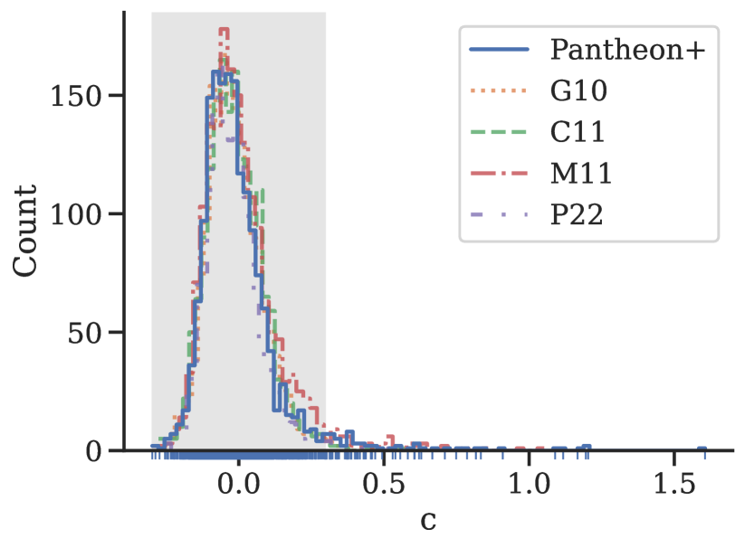
Figure 1: SALT2 colour distribution for our final data set ($N=1686$). We are still dominated by cosmological SNe Ia (gray shaded region, $-0.3<c<0.3$). This sample has 57 more SNe Ia than Pantheon+: 51 have $0.3<c\leq 1.0$ and 6 have $c>1.0$. The mean of the cosmological sample and the full sample are $c=-0.021$ and $c=-0.002$ respectively. The SALT2 training set has a mean color of 0, by definition. Simulations of the Pantheon+ catalogue using four scatter models (G10, C11, M11, and P22) of SNe Ia are also shown.

For this analysis, we remove the requirement that SN Ia have $c\leq 0.3$. We do, however, keep all the other quality cuts as defined in Scolnic et al. (2021). We simplify the FITPROB cut from Pantheon+, by only ensuring that FITPROB is non-zero instead of using survey specific cuts. We present the distribution of SALT2 colour in Figure 1. There are 57 more SNe Ia than in Pantheon+: 1686 in total, 51 have $0.3<c\leq 1.0$ and 6 have $c>1.0$. Beyond these 57 SNe Ia, Pantheon+ also cuts SNe Ia at the bias correction stage, something not addressed in this work. A similar distribution is seen in the volume limited sample from the Zwicky Transient Facility Bright Transient Survey (Sharon & Kushnir, 2022).

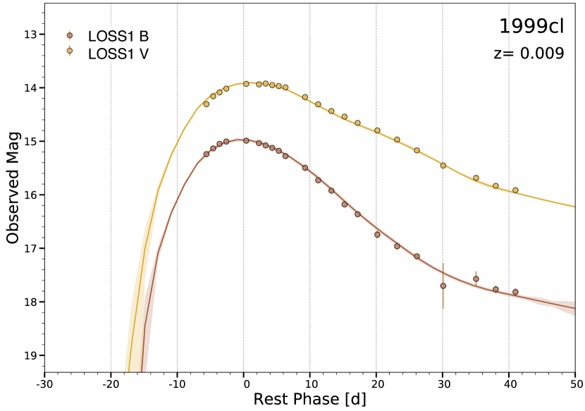
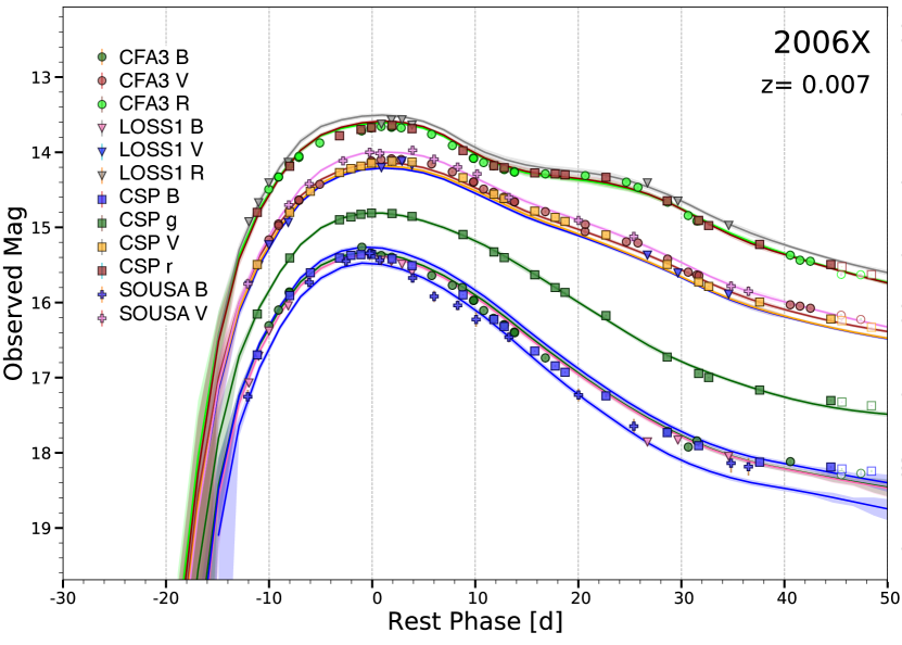
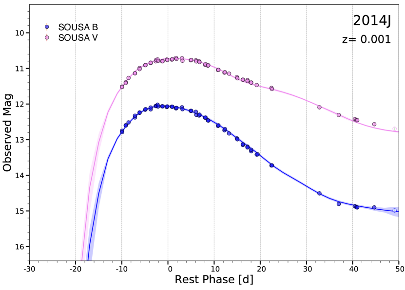
Figure 2: SALT2 light-curve fits for three representative extremely reddened SN Ia ($c>1$). The SALT2 model is not trained on SN Ia with $c>0.3$. However, SN1999cl (left), SN2006X (center), and SN2014J (right) have excellent SALT2 fits, even with $c$ values of $1.09\pm 0.04$, $1.19\pm 0.03$, $1.20\pm 0.05$ respectively.

The full Pantheon+ data set includes SN Ia observed from multiple telescopes. These are recorded, initially, as separate events to allow for cross-survey calibrations. However, for this analysis, they are combined into a single object. If the same SN Ia is observed by multiple telescopes, we set the colour and light-curve shape to be the mean of the observations. For the uncertainties on the average parameter, we take the maximum of the individual uncertainties or the range between the individual fits, whichever is greater. This ensures our final uncertainty encompasses all individual point estimates. In the Pantheon+ data release, there are two SNe Ia with data from four surveys (SN2006X and SN2007af). For these objects, we allow ourselves to reject one survey if the light-curve fits disagrees with the other three surveys. Following this reasoning, we remove the SWIFT data on SN2006X. We do not find similarly obvious discrepancies for SN Ia with data from three surveys.

We inspect the quality of the fits for several highly-reddened SNe Ia because of the concern that the light-curve model is not valid at this colour range. In Figure 2, we show three representative light curves of extremely reddened SN Ia: SN2014J ($c=1.20$), SN1999cl ($c=1.09$), and SN2006X ($c=1.17$). These SN Ia were selected for presentation prior to seeing their light curves. They all have excellent SALT2 fits, even with $c$ values $>$1.

We looked at the percent of SNe Ia that pass the light-curve FITPROB cut described in Scolnic et al. (2021). In general, red SNe Ia ($c>0.3$) have a lower percent of passing, from a $\sim$90% to a $\sim$80% pass rate. The highly reddened SNe Ia have some colour regions with a low percent of passing this quality cut ($\sim$60% at $c\sim 0.5$) but other regions where 70%–100% pass ($0.6<c<1.4$), implying the trustworthiness of light-curve fits resulting in $c>0.3$. The increase in fit quality after $c=0.5$ is likely do to stochastic effects since there are only $\sim$4 SNe Ia per $\Delta c=0.1$ bin at this point in the population distribution (Figure 1).

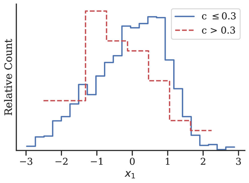
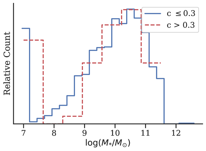
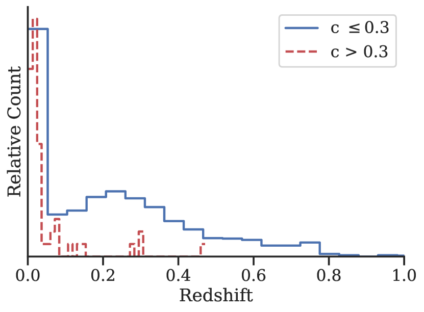
Figure 3: Distributions of SN Ia light-curve shape (left), host galaxy stellar mass (center), and redshift (right) for the cosmological and highly reddened sub-samples. Using the two-sample Kolmogorov-Smirnov test, we see a difference in $x_{1}$ ($3.0\sigma$) and redshift ($>$5$\sigma$) between these two samples, but not in stellar mass ($0.5\sigma$).

We show in Figure 3 the light-curve shape ($x_{1}$), host galaxy stellar mass ($M_{\star}$, in units of $\log(M_{\sun})$), and redshift distributions for the cosmological sample and the highly reddened sample. The reddened sample’s $x_{1}$ distribution changes significantly compared to the cosmological sample ($3.0\sigma$, via a two-sample Kolmogorov-Smirnov test), due to a relative increase of fast decliners ($x_{1}<0$). This shift in the $x_{1}$ population is not likely to be from an enhanced selection effect, since SNe Ia with negative $x_{1}$ are fainter on average. We speculate that this shift may be the result of a change in the host-galaxy population, although not a different stellar mass distribution, as seen below. It has been previously shown that $x_{1}$ is correlated with host galaxy properties (e.g., Hamuy et al., 2000), and that for any given galaxy, the apparent $x_{1}$ distribution is smaller than it is for the SNe Ia population as a whole (Scolnic et al., 2020). Alternatively, highly reddened SNe Ia may have an enhanced SN1991bg-like population. The redshift distributions also differ ($>$5$\sigma$). This is due to the increased effect of selection effects on highly reddened SNe Ia, resulting in a redshift distribution that favours low redshifts. However, the $M_{\star}$ distributions are consistent between these two samples ($0.5\sigma$).

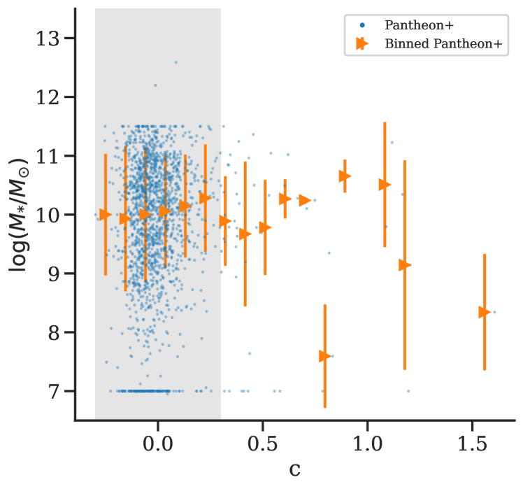
Figure 4: Host galaxy stellar mass as a function of SALT2 $c$. In bins of colour, the orange triangles show the median $\log(M_{*}/M_{\odot})$ and the uncertainty of the points show the robust scatter. At large values of $c$, the relative decrease of SNe Ia adds statistical noise, but the red SNe Ia are not found in a substantially different host galaxy population than the cosmological sample (gray shaded region). The lines at 11.5 and 7 are artefacts of the stellar mass fitting process. A value of 7 was given when a mass was indeterminable due to faint photometry. A value of 11.5 was given when the mass is sufficiently large to be extremely unlikely to be less than 10. Some masses are larger than 11.5 because they are from surveys that don’t follow the previous convention.

In Figure 4, we show the host galaxy stellar mass distribution as a function of SALT2 colour. At highly reddened colours, the relative decrease of SNe Ia adds statistical noise, but the red SNe Ia are not found in a substantially different host galaxy population than the cosmological sample.

2.3 Simulations

We use simulations of the Pantheon+ data set generated by the SNANA simulation software (Kessler et al., 2009b, 2019) with the PIPPIN (Hinton & Brout, 2020) wrapper. A brief overview of SNANA is as follows: 1) fluxes are generated from a source model (SALT2, Taylor et al. 2021), with noise and detection characterized in survey-specific methods alongside a rest-frame SED for each epoch that is subject to cosmological and galactic effects, 2) the SED is integrated for each filter to obtain broadband fluxes, which are further subjected to survey-specific measurement noise, and 3) candidate logic and spectroscopic identification efficiencies are applied. For this paper, we take our Pantheon+ simulation inputs from Brout et al. (2022), a brief overview of which is presented in Table 2 of Popovic et al. (2021a).

3 Method

In this work, both $R_{V}$ and $\beta$ represent a relationship between colour and luminosity. $\beta$ is a fit parameter used with SN Ia data and empirical models like SALT2, whereas $R_{V}$ is a physical property and used in forward model simulations. Therefore, a colour dependence of $R_{V}$ can be seen as a colour dependence of $\beta$.

We perform two types of fits on the Pantheon+ data. The first model assumes a single $\beta$ for the whole sample. This is described in Section 3.1. The second is a broken-linear model where $\beta$ can change after a certain colour value, to test the predictions of M11 and others that the colour-luminosity relationship is colour dependent (Section 3.2). We also discuss how we measure the scatter around the colour-luminosity relation in Section 3.3. Finally, we present four models of the intrinsic scatter of SNe Ia brightnesses, including possible colour dependence of $R_{V}$, we use in our forward model simulations (Section 3.4).

3.1 Colour-luminosity Relationship

We modify Equation 2 in order to define a non-colour corrected absolute magnitude (M^′) per SN Ia:

$$\mathrm{M}^{\prime}\equiv m_{B}-\mu(z,\mathrm{cosmology})+\alpha x_{1}~{}.$$ (3)

To focus this work on understanding $\beta$, we do not fit for either the cosmology or $\alpha$. Instead, we assume a flat $\Lambda$CDM cosmology of $h=0.70$, $\Omega_{M}=0.3$, $\Omega_{\Lambda}=0.7$ and use $\alpha=0.15$. These are similar to those derived from the Pantheon+ cosmological analysis (Brout et al., 2022). We note that in Equation 3 and throughout, no bias corrections are applied to any distance-like estimates.

3.2 Modelling the Colour-Luminosity Relationship

We introduce two models of the colour-luminosity relation to fit $\mathrm{M}^{\prime}$ defined in Equation 3: a linear one and a broken-linear one. Our linear one is defined such that

$$\mathrm{M}^{\prime}_{\mathrm{mod}}=\beta c~{}+\mathrm{M}^{{}^{\prime}}_{0}$$ (4)

where $\mathrm{M}{{}^{\prime}}_{0}$ is the absolute magnitude of a $c=0$ SN Ia and $\mathrm{M}^{\prime}_{\mathrm{mod}}$ is the model’s prediction for $\mathrm{M}^{\prime}$.

For the broken-linear model, we build a LINMIX-like (Kelly, 2007) Bayesian Hierarchical model (BHM) around the equation:

$$\mathrm{M}^{\prime}_{\mathrm{mod}}=\begin{cases}\beta c+\mathrm{M}^{{}^{\prime}}_{0}\hfill&\text{if}\,c\leq c_{\mathrm{break}}\\ (\beta+\Delta_{\beta})c+\mathrm{M}^{{}^{\prime}}_{0}-c_{\mathrm{break}}\Delta_{\beta}\quad&\text{if}\,c>c_{\mathrm{break}}\\ \end{cases}$$ (5)

where $\Delta_{\beta}$ is the change in the slope between the cosmological and highly reddened SN Ia. The $-c_{\mathrm{break}}\Delta_{\beta}$ term allows for the piecewise function to remain continuous at $c=c_{\mathrm{break}}$. In the fiducial analysis $c_{\mathrm{break}}=0.3$.

This model is partially derived from UNITY (Rubin et al., 2015). A full description of the BHM used can be seen in Appendix A. To fit for $\beta$, we use a Python port of the IDL package LINMIX_ERR (Kelly, 2007). We take advantage of two mathematical characteristics of LINMIX. First, it is Bayesian and naturally provides uncertainties on the model parameters. Secondly, it handles two-dimensional measurement uncertainties.

3.3 Residual Scatter

The best fit results from the models presented in Sections 3.1 and 3.2 will still result in residual scatter. The scatter in SN Ia absolute magnitude is a common diagnostic (e.g., BS21, ). For this work, we will calculate the root-mean-squared (RMS) scatter of the residuals as a function of colour to diagnose if this scatter is constant with colour, or if red SNe Ia have an increased scatter. An increase in scatter as a function of colour is a prediction of the variable $R_{V}$ model of BS21.

3.4 Forward Modelling Different Scatter Models

Simulating SN Ia data sets require an empirical model to describe brightness variations among the SN Ia population, or intrinsic scatter. In this work, we use four different scatter models—Guy et al., 2010 (G10), Chotard et al., 2011 (C11), the Popovic et al., 2021a (P22) fits for BS21, and Mandel et al., 2011 (M11). Both G10 and C11 are spectral variation models, though they differ in the amount of variation ascribed to chromatic scatter. G10 attributes approximately 70% of scatter to achromatic effects, with the rest coming from chromatic sources. C11 only 25% of scatter is achromatic, and the remaining 75% is from chromatic effects.

In contrast to G10 and C11, P22 and M11 do not have an explicit SED variation; instead, P22 and M11 ascribe scatter to dust effects. We use the updated BS21 model parameters from P22 for this paper. This assumes no relationship between $E(B-V)$ and $R_{V}$. We implement the M11 model by replacing the $R_{V}$ and $E(B-V)$ relationships from P22 with those from Mandel et al. (2011):

$$\frac{1}{R_{V}}=0.36+0.14A_{V}$$ (6)

with a Gaussian scatter around this mean $\frac{1}{R_{V}}$ of $\sigma=0.04$ (Mandel et al., 2011).

4 Results

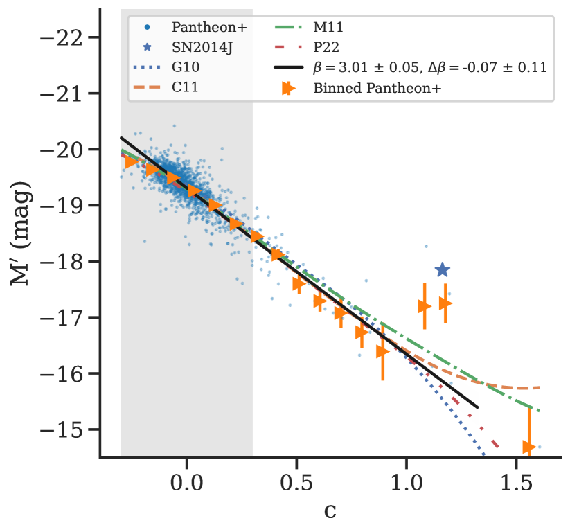
Figure 5: Colour-luminosity plot for our full sample (blue), including 57 highly reddened SN Ia. Bins in colour show the median $\mathrm{M}^{{}^{\prime}}$ (with error bars showing the RMS divided by the square-root of the number of objects per bin, orange). The median (and $1\sigma$) broken-linear model is shown in black. We find $\beta=3.01\pm 0.05$ and $\Delta\beta=-0.07\pm 0.11$. This is consistent with only one slope across this whole range. We also present the non-parametric kernel regression of the median luminosities for each scatter model (G10, blue-dotted line; C11, orange-dashed line; M11, green-dot-dashed line; P22, red-dot-dot-dashed line.) We note that SN2014J (blue star) is significantly brighter than the trend, as expected for its low $R_{V}$ value. The gray shaded region is the traditional cosmological sample.

We show the colour-luminosity plot for the Pantheon+ data set (including the highly reddened SNe Ia) in Figure 5. In addition to the data, we show equally sized colour bins of the median luminosity and root-mean-square (RMS) divided by the square-root of the number of objects per bin. We also plot the non-parametric kernel regression of the median luminosities for each scatter model. We use a variant of Nadaraya-Watson kernel regression (Nadaraya, 1964; Watson, 1964) that uses a local linear regression estimator, as implemented in the Python package statsmodels (Seabold & Perktold, 2010).

4.1 Measuring $\beta$

$c_{\mathrm{break}}$	$\beta$	$\Delta_{\beta}$	Significance
0.0	$2.64\pm 0.06$	$0.49\pm 0.08$	6.1$\sigma$
0.2	$2.96\pm 0.05$	$0.08\pm 0.10$	0.8$\sigma$
0.3	$3.01\pm 0.05$	$-0.07\pm 0.11$	0.6$\sigma$
0.4	$3.03\pm 0.05$	$-0.20\pm 0.12$	1.7$\sigma$
0.5	$3.03\pm 0.05$	$-0.28\pm 0.13$	2.2$\sigma$

Table 1: $\beta$ and $\Delta_{\beta}$ values for various broken-linear break points (Equation 5). The fiducial analysis breaks at $c=0.3$ because that is the typical cosmological cut.

Following the procedure described in Section 3.1, we calculate a single $\beta$ with a median plus or minus the robust scatter: $\beta=2.98\pm 0.04$. For the broken-linear BHM, described in Section 3.2, we see a consistent slope above and below the $c=0.3$ split. We find $\beta=3.01\pm 0.05$ and $\Delta_{\beta}=-0.07\pm 0.11$, resulting in a $\beta(c>0.3)=2.94\pm 0.12$. This is a $<$0.7$\sigma$ deviation from a constant linear trend. The result of our BHM can be seen plotted along with the data in Figure 5. All model parameters are well constrained, with $\beta$ and $\Delta_{\beta}$ being the only model parameters showing a notable correlation. For the full details of the fit, see Appendix B.

We present the $\beta$ and $\Delta_{\beta}$ estimates for several values of $c_{\mathrm{break}}$ in Table 1. Between $0.2\leq c_{\mathrm{break}}\leq 0.5$ there are no significant $\Delta_{\beta}$ values. However, there is a very significant shift in $\beta$ at $c=0$. A shift in $\beta$ at $c=0$ has been seen multiple times before (Scolnic et al., 2014; Rubin et al., 2015). This shift is thought to be a transition of the observed color being dominated from intrinsic color to dust.

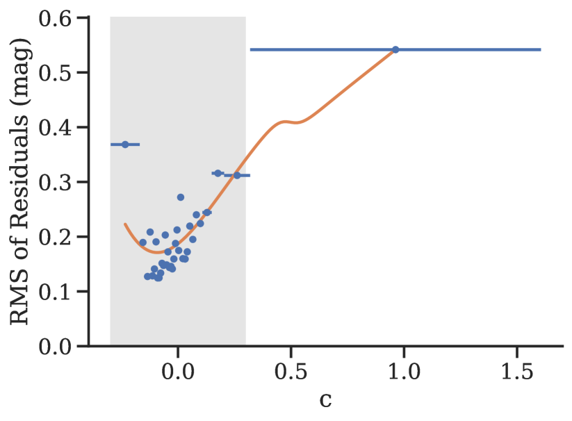
Figure 6: The root-mean-squared (RMS) scatter of the residuals between the data and the median broken linear model ($\beta=3.01$ and $\beta(c>0.3)=2.94$). Each bin is evenly filled with 50 objects each. Highly reddened SN Ia have more scatter than the cosmological sample. However, they do appear to continue the trend seen in the red half ($c>0$) of the cosmological sample. The full cosmological sample is denoted by the shaded region. A non-parametric kernel regression is plotted in orange. It smooths and interrelates between the points. We also calculated the robust scatter of the residual to see if this trend was dominated by outliers. Though the value of the scatter decreased, the trends seen in this plot did not change.

In Figure 6, we present the RMS scatter of the residuals vs colour. Each bin is evenly filled with 50 objects each. This allows for robust measurements of the RMS while distinguishing the highly reddened ($c>0.3$) SNe Ia from the cosmological sample. Highly reddened SN Ia have larger scatter than the cosmological sample. However, they continue the trend seen in the red half ($c>0$) of the cosmological sample. We use the same statsmodels kernel regression method to smooth and interpolate between the points. This trend is robust to changes in bin size. We also calculate the robust scatter of the residuals to verify that the observed trend is resilient to outliers. Though the value of the scatter decreases, the trends seen in this plot do not change. An increasing RMS with colour is predicted by the BS21 model, but G10 and C11 both assume a constant scale of remaining scatter with colour.

4.2 Comparison of Forward Model Simulations

We check the four scatter models described in Section 3.4 to determine which best matches the Pantheon+ data. To quantify this agreement, we take inspiration from the metrics presented in P22. We have one metric related to the distribution of $c$ and one related to the colour-luminosity relationship.

The first metric describes the relative number of SNe Ia with red colours and compares the predictions from simulations using different scatter models to the data. By using the scatter models from G10 and C11 with asymmetric Gaussian colour distributions (Scolnic & Kessler, 2016; Popovic et al., 2021b), we find that simulations with these models predict no $c>1$ SN Ia. This can be seen in colour histograms of the simulations in Figure 1. In fact, a $c>1$ SN Ia would be a $>$9$\sigma$ outlier. The Pantheon+ data set has 6 SNe Ia with $c>1$. On the other hand, the P22 model is based on an exponential dust distribution, and therefore simulations with this model predict more SNe Ia at redder colours, which better matches the data.

In order to quantify these colour-distribution predictions, we calculate a $\chi^{2}$ defined as:

$$\chi^{2}_{c}=\sum_{i}^{N_{\mathrm{bins}}}\frac{(N_{\mathrm{data,i}}-N_{\mathrm{sim,i}})^{2}}{\sigma_{\mathrm{Poisson,i}}^{2}}$$ (7)

where $N_{i}$ is the number of observed SN Ia per bin in either the data or simulation, and $\sigma_{\mathrm{Poisson}}$ is the typical Poisson counting uncertainty on the data bins ($\sqrt{N_{\mathrm{data}}}$).

	$\chi^{2}_{c}$	$\chi^{2}_{\mathrm{M}^{{}^{\prime}}}$	$\chi^{2}_{\mathrm{M}^{{}^{\prime}}},~{}c<1.0$
	($N_{\mathrm{bins}}=20)$	($N=1686$)	($N=1680$)
P22	38.3	1566.8	1537.9
M11	58.6	1568.8	1551.2
C11	45.2	1561.6	1538.4
G10	45.2	1580.5	1537.6

Table 2: $\chi^{2}$ Between Forward Model Simulations and the Pantheon+ Data Set

We also calculate a $\chi^{2}$ for the colour-luminosity relationship. This compares the data ($\mathrm{M}^{{}^{\prime}}_{i}$) to the kernel regression smoothed luminosity ($\mathrm{M}^{{}^{\prime}}_{\mathrm{sim}}(c_{i})$) of each simulation with the uncertainty coming from the measured scatter in the data:

$$\chi^{2}_{\mathrm{M}^{{}^{\prime}}}=\sum^{N}_{i}\frac{\left[\mathrm{M}^{{}^{\prime}}_{i}-\mathrm{M}^{{}^{\prime}}_{\mathrm{sim}}(c_{i})-\Delta\mathrm{M}_{0}\right]^{2}}{\mathrm{RMS}(c_{i})}$$ (8)

where $\mathrm{RMS}(c_{i})$ is the kernel regression smoothed for a given SN Ia colour ($c_{i}$), as presented in Figure 6. $\Delta\mathrm{M}_{0}$ is a single number for the whole dataset and is a shift in absolute magnitude of an $x_{1}=c=0$ SN Ia. This is calculated as the median of $(\mathrm{M}^{{}^{\prime}}_{i}-\mathrm{M}^{{}^{\prime}}_{\mathrm{sim}}(c_{i}))$ and is up to 0.1 mag, due to the different definitions used when defining different scatter models.

Our results are shown in Table 2. When looking at the colour distribution, P22 matches the data the best. G10 and C11 match the data better than M11, even though they see $c>1$ SN Ia as $>$9$\sigma$ outliers. For the colour-luminosity relationship, C11 does the best, but P22 and M11 have a similar $\chi^{2}$. Cutting the low statistic $c>1.0$ data range, G10, P22 and C11 are all within a $\Delta\chi^{2}$ of $<$1.

5 Discussion

5.1 Low $R_{V}$ SN Ia in the Literature

Though we find a consistent $\beta$ for Pantheon+ across a wide range of SN Ia colours, there are well measured highly reddened individual SN Ia, such as SN2014J, with low $R_{V}$ values ($R_{V}\sim 1.5$, Amanullah et al., 2015). In Figure 5, we show that SN2014J is above the measured $\beta$. We see individual SNe Ia with low $R_{V}$, even though the mean for the data set ($\beta$) is higher, which implies there is a range of $R_{V}$ values.

SN Ia	c	Stellar Mass	$\Delta\mathrm{mag}$	$R_{V}$	Reference
		$\log(M_{*}/M_{\sun})$	mag
1999cl	1.09	9.9	-1.25	$1.55\pm 0.08$	K06
2002bo	0.32		0.77	$1.00\pm 0.10$	ER06
				$1.22^{+0.26}_{-0.21}$	P13
				$1.1$	C16
2006X	1.17	10.3	-0.46	$1.31^{+0.08}_{-0.1}$	P13
2008fp	0.30	10.5	0.77	$1.20^{+0.26}_{-0.14}$	P13
2012cg	0.11	9.6	1.60	$2.7^{+0.9}_{-0.7}$	A15
2014J	1.16		-0.71	$1.4\pm 0.1$	A15

Table 3: Pantheon+ SNe Ia with $R_{V}$ Measurements in the Literature. Stellar mass and $c$ are from the Pantheon+ data release. $\Delta\mathrm{mag}$ is the residual between M^′ and the trend line presented in Figure 5.
References: A15 (Amanullah et al., 2015); C16 (Cikota et al., 2016); ER06 (Elias-Rosa et al., 2006); K06 (Krisciunas et al., 2006); P13 (Phillips et al., 2013).
^∗A SN Ia with $z<0.01$ and $c>0.3$.

In Table 3, we present a table of six SNe Ia with $R_{V}$ measurements from the literature. In this table we include the colour and host galaxy stellar mass from Pantheon+ as well as the residual from the median fit presented in Figure 5 ($\beta=3.01\pm 0.05$ and $\Delta_{\beta}=-0.07\pm 0.11$). SN1999cl, SN2006X, SN2012cg, and SN2014J all follow the expected trend of brighter residuals for lower $R_{V}$. However, a conclusion is hard to draw, both due to the low number of objects and that SN2002bo and SN2008fp do not follow this trend.

5.2 Improving $\text{H}_{0}$

Previous studies have raised that a variable $R_{V}$ may affect measurements of $\text{H}_{0}$. Mortsell et al. (2021) derived a colour-luminosity relation for each Cepheid host galaxy individually, though with large uncertainties. Directly measuring the line-of-sight $R_{V}$ for Cepheid and SNe Ia, especially with dust dominated, highly reddened SNe Ia, would provide an interesting comparison and illuminate whether the dust around SNe Ia is interstellar or circumstellar.

SN Ia	Host Galaxy	Redshift	c
2014J	M82	0.00138	1.16
1996ai	NGC 5005	0.00451	1.61
2002bo	NGC 3190	0.00613	0.32
2017drh	NGC 6384	0.00616	1.22
2008fp	ESO 428-G14	0.00618	0.31
2006X	M100	0.00664	1.17
1997dt	NGC 7448	0.00683	0.47
2007bm	NGC 3672	0.00727	0.38
1996bk	NGC 5308	0.00779	0.33
1999cl	M88	0.00850	1.09

Table 4: Possible $\text{H}_{0}$ Calibrators. We present all $c>0.3$ SNe Ia with $z<0.01$ (N=10). A total of 17 highly-reddened SNe Ia are available if calibration is possible to $z<0.015$ or $\mu\lesssim 34~{}\text{mag}$. This table excludes Pantheon+ SNe Ia with $c<0.3$ but are not typical $\text{H}_{0}$ calibrators, such as SN1989B ($c=0.298\pm 0.038$) and SN1998bu ($c=0.261\pm 0.025$).

Furthermore, without the $c<0.3$ cut, there is an increased number of $\text{H}_{0}$ calibrators ($z<0.01$ SN Ia where either Cepheid or Tip of the Red Giant Branch distances are possible, Freedman et al. 2019) by 10—see Table 4 for a full list. There are 17 possible calibrators if we extend this to $z<0.015$ or $\mu\sim 34$. The latest $\text{H}_{0}$ measurement, by the SH0ES collaboration, contains 42 Cepheid-calibrated SN Ia (Riess et al., 2021). The rate of new SN Ia calibrators is $\sim 1/\mathrm{year}$, so these highly reddened SN Ia pose a promising method to increase the precision of the local measurement of $\text{H}_{0}$, which can be forecasted using the precision per SN Ia with redder colours as seen in Figure 6.

6 Conclusions

Though SALT2 was optimized in the cosmological colour range ($-0.3<c<0.3$) it still has good agreement with the data out to $c>1$. We see no evidence for future research to cut at $c=0.3$, but suggest consideration of the use of SN Ia with $c\lesssim 1$.

We find a consistent slope between $c<0.3$ and $c>0.3$ ($\Delta_{\beta}=-0.07\pm 0.11$). Measurements of redder SNe Ia do have a larger post standardization scatter, but they follow a trend between RMS and colour also seen in the cosmological sample and explained by BS21. A limit in colour is still needed to avoid low number statistics where we will not be able to constrain the variability in $R_{V}$. Highly reddened SN Ia can be included in cosmological samples, or at least used for constraining systematic uncertainties in the more statistically powerful samples.

Our results strongly support that $R_{V}$ varies across the SNe Ia population, and must be accounted for in cosmological analyses. The P22 scatter model matches the colour distribution best, with C11, P22 and M11 matching the colour-luminosity relationship about equally. Additionally, the correlation between the spectroscopicly measured $R_{V}$ of SNe Ia and their residual scatter is inconclusive. However, we note this is from only six SNe Ia and would benefit from a larger sample.

Finally, we want to conclude by reiterating that highly reddened SNe Ia are highly affected by selection effects. A good model of these effects is required for any study of them or perform analyses with them.

Data Availability

This work uses the Pantheon+ data set. The Pantheon+ data set is available at pantheonplussh0es.github.io. The associated PyMC3 model can be found at github.com/benjaminrose/Investigating-Red-SN. Any other data requests can be directed to the lead author.

Appendix A Full Description of the Broken-linear Model

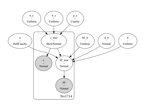
Figure 7: A probabilistic graphical model of our broken-linear BHM. Each observed parameter ($c$ and $M^{\prime}$) are drawn from Normal distributions with means of their true parameters (${c}_{\mathrm{true}}$, ${M^{\prime}}_{\mathrm{true}}$) and standard deviations of their measurement errors. There is one of each of these four parameters for every observed SN Ia ($N=1686$). The broken-linear relationship between ${c}_{\mathrm{true}}$ and ${M^{\prime}}_{\mathrm{true}}$ is parameterized by an intercept ($M^{\prime}_{0}$), angle of the $-0.3\leq c\leq 0.3$ line ($\theta$) and change of this angle after $c>0.3$ ($\Delta_{\theta}$). ${M^{\prime}}_{\mathrm{true}}$ forms a Normal distribution around a mean of this broken-linear relationship, with a scatter outside the model of $\sigma$. The ${c}_{\mathrm{true}}$ skew-normal distribution parameters ($\mu_{c}$, $\sigma_{c}$, $\alpha_{c}$) are fit along with the broken-linear parameters.

We built a Bayesian Hieratical model (BHM), imitating LINMIX, but using the broken-linear relationship of Equation 5. For this model, we fit the broken linear in the “true" parameter space. These “true” parameters are the model’s estimation of $c$ and $\mathrm{M}^{\prime}$ without the effects of observational noise. Each observed $c$ and $\mathrm{M}^{\prime}$ are drawn from normal distributions ($\mathcal{N}$) with means of ${c}_{\mathrm{true}}$ and ${\mathrm{M}^{\prime}}_{\mathrm{true}}$ and standard deviations equal to the measurement uncertainties ($\sigma_{\mathrm{M}^{\prime}}$ and $\sigma_{c}$)

$$\mathrm{M}^{\prime} \sim\mathcal{N}({\mathrm{M}^{\prime}}_{\mathrm{true}},~{}\sigma_{\mathrm{M}^{\prime}}^{2}),$$ (9)

$$c \sim\mathcal{N}({c}_{\mathrm{true}},~{}\sigma_{c}^{2}).$$ (10)

The relationship between ${c}_{\mathrm{true}}$ and ${M^{\prime}}_{\mathrm{true}}$ (Equation 5) is such that a unique unexplained scatter term ($\epsilon$) is applied to each observation. This is Equation 1 in Kelly (2007). $\epsilon$ is drawn from a normal distribution with a mean of zero and a variance of $\sigma^{2}$ ($\epsilon\sim\mathcal{N}(0,~{}\sigma^{2})$). Therefore,

$${\mathrm{M}^{\prime}}_{\mathrm{true}}\sim\mathcal{N}(f({c}_{\mathrm{true}},\beta,\Delta\beta,\mathrm{M}^{\prime}_{0}),~{}\sigma^{2}),$$ (11)

where the mean of each ${\mathrm{M}^{\prime}}_{\mathrm{true}}$ is defined by Equation 5, ${c}_{\mathrm{true}}$, and the three broken-linear parameters ($\beta$, $\Delta_{\beta}$, $\mathrm{M}^{\prime}_{0}$).

We are able to make one significant simplification compared to LINMIX. Instead of using a Gaussian mixture model to describe of the distribution of the independent variable, $c$, we are able to use a skew normal. Though population parameters have been fit in Scolnic & Kessler (2016) and Popovic et al. (2021b), our BHM marginalizes over these variables. Following the parameterization of the population distribution of $c$ as a skew normal (Rubin et al., 2015), we are able to reduce the number of population parameters from six (in LINMIX) to three. Therefore, each true $c$ value (${c}_{\mathrm{true}}$) is drawn from a skew normal distribution where the mean, standard deviation, and skewness parameters ($\mu_{c}$, $s_{c}$, $\alpha_{c}$ respectively) are fit along with the broken-linear parameters to avoid biases (Gull, 1989). We present our model visually in Figure 7. This model differs from LINMIX and Rubin et al. (2015) by ignoring correlations between the observed parameters.

For fitting, we do a simple transformation of variables from slope ($\beta$) to angle of line above horizontal ($\theta\equiv\arctan(\beta)$). A uniform prior in slope preferentially searches larger values. As described by VanderPlas (2014), an uniformed prior is achieved with either a transform of the variables, like above, or the use of invariant Jeffreys priors (Jeffreys, 1946). When possible, we use non-informative priors, except when required for an unbiased result (Gull, 1989). We present our priors in Table 5. A PyMC3 (Salvatier et al., 2016) implementation of this model and our associated analysis scripts can be found at https://github.com/benjaminrose/Investigating-Red-SN.

Variable	Name	Distribution
$\mathrm{M}^{\prime}_{0}$	Absolute magnitude for an $x_{1}=c=0$ SN Ia	Uniform($-19.4,~{}-19.2$)
$\theta$	Slope of color-luminosity relationship	Uniform($1.2,~{}1.45$)
$\Delta_{\theta}$	Change in color-luminosity relationship slope	$\mathcal{N}(0,~{}0.15^{2})$
$\sigma$	Scatter in data from outside the model	HalfCauchy($0.05$)
${c}_{\mathrm{true}}$	Estimated SN Ia color without measurement noise	SkewNormal($\mu_{c},~{}\sigma^{2}_{c},~{}\alpha_{c}$)
$\mu_{c}$	Mean of ${c}_{\mathrm{true}}$ distribution	Cauchy($0,~{}0.3$)
$\sigma_{c}$	Standard deviation of ${c}_{\mathrm{true}}$ distribution	Uniform($0.01,~{}0.2$)
$\alpha_{c}$	Skewness of ${c}_{\mathrm{true}}$ distribution	Uniform($-0.1,~{}2.0$)

Table 5: Parameters, and their priors, used in the borken-linear BHM.

Appendix B Detailed Results of the Broken-linear Fit

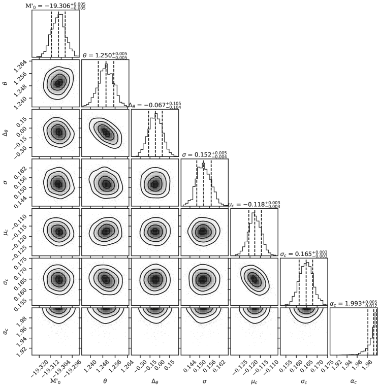
Figure 8: A corner plot representation of seven posterior parameters. Nothing is correlated except theta and delta-theta. We do hit the edge of the colour skewness parameter, but with a good predictive posterior (Figure 9) we conclude that this is sufficient.

We present a corner plot of the model parameters in Figure 8. All parameters are well fit ($\hat{R}=1.0$). $\alpha_{c}$ hits the prior bounds. This makes sense, since we find that Gaussian tails are not a good description for the extremely red SNe Ia. In addition, there is a strong correlation between $\theta$ and $\Delta_{\theta}$. We expect the slightly higher unexplained scatter ($\sigma=0.19\pm 0.01~{}\text{mag}$) because we do not perform a full fit, i.e., the light-curve shape standardization coefficient is fixed to $\alpha=0.15$.

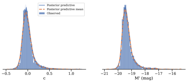
Figure 9: The posterior predictive distribution for the model described in Sections 3.2, A and 7. The posterior predictive distribution is the BHM prediction of the observed parameter distributions (orange dashed line). This is done by marginalizing over the model parameters to get the probability of a new data set (orange dashed line), given the original data set (blue histograms). We see that the model is able to reproduce the observed distributions of $c$ (left) and $M^{\prime}$ (right).

By marginalizing over the model parameters, we are able to create a probability distribution of new data ($\vec{x}$) given the observed data ($\mathscr{X}$), $P(\vec{x}|\mathscr{X})$. This is the posterior predictive distribution. In Figure 9, via the posterior predictive distribution, we see that the model can accurately recreate the observed distributions of $c$ and $M^{\prime}$ implying that our parameterization of the population distributions (i.e., $\mu_{c}$, $s_{c}$, $\alpha_{c}$) are sufficient.

As an additional validation, we fit the broken linear model on the P22 simulations directly. We successfully recovered $\beta=3.04\pm 0.01$ and $\Delta_{\beta}=-0.31\pm 0.55$, for a simulation with $\beta=3.10$ across the entire colour range.

References

- Al-Rfou et al. (2016) Al-Rfou R., et al., 2016, arXiv e-prints, abs/1605.02688
- Amanullah et al. (2015) Amanullah R., et al., 2015, Mon. Not. R. Astron. Soc., 453, 3301
- Astropy Collaboration (2013) Astropy Collaboration 2013, A&A, 558, A33
- Astropy Collaboration (2018) Astropy Collaboration 2018, Astronomical Journal, 156, 123
- Betoule et al. (2014) Betoule M., et al., 2014, A&A, 568, A22
- Brout & Scolnic (2021) Brout D., Scolnic D., 2021, ApJ, 909, 26
- Brout et al. (2021) Brout D., et al., 2021, arXiv:2112.03864 [astro-ph]
- Brout et al. (2022) Brout D., Scolnic D., Vincenzi M., Dwomoh A., Lidman C., Riess A., Ali N., Dai M., 2022, in prep.
- Brownsberger et al. (2021) Brownsberger S., Brout D., Scolnic D., Stubbs C. W., Riess A. G., 2021, arXiv e-prints, p. arXiv:2110.03486
- Burns et al. (2014) Burns C. R., et al., 2014, ApJ, 789, 32
- Cardelli et al. (1989) Cardelli J. A., Clayton G. C., Mathis J. S., 1989, The Astrophysical Journal, 345, 245
- Carr et al. (2021) Carr A., Davis T. M., Scolnic D., Said K., Brout D., Peterson E. R., Kessler R., 2021, arXiv e-prints, p. arXiv:2112.01471
- Chen et al. (2022) Chen R., et al., 2022, Measuring Cosmological Parameters with Type Ia Supernovae in redMaGiC Galaxies (arXiv:2202.10480)
- Chotard et al. (2011) Chotard N., et al., 2011, A&A, 529, L4
- Cikota et al. (2016) Cikota A., Deustua S., Marleau F., 2016, Astrophysical Journal, 819, 152
- DES Collaboration et al. (2019) DES Collaboration et al., 2019, ApJL, 872, L30
- De Marchi et al. (2021) De Marchi G., Panagia N., Milone A. P., 2021, arXiv e-prints, p. arXiv:2109.13914
- Elias-Rosa et al. (2006) Elias-Rosa N., et al., 2006, Monthly Notices of the Royal Astronomical Society, 369, 1880
- Foreman-Mackey (2016) Foreman-Mackey D., 2016, JOSS, 24
- Freedman et al. (2019) Freedman W. L., et al., 2019, ApJ, 882, 34
- Garnavich et al. (1998) Garnavich P. M., et al., 1998, ApJ, 509, 74
- Gonzalez-Gaitan et al. (2021) Gonzalez-Gaitan S., de Jaeger T., Galbany L., Mourao A., Paulina-Afonso A., Filippenko A. V., 2021, Monthly Notices of the Royal Astronomical Society, 508, 4656
- Goobar (2008) Goobar A., 2008, The Astrophysical Journal Letters, 686, L103
- Guillochon et al. (2017) Guillochon J., Parrent J., Kelley L. Z., Margutti R., 2017, Astrophysical Journal, 835, 64
- Gull (1989) Gull S. F., 1989, in An International Book Series on The Fundamental Theories of Physics: Their Clarification, Development and Application, Vol. 36, Maximum Entropy and Bayesian Methods. Fundamental Theories of Physics. Springer, Dordrecht
- Guy et al. (2007) Guy J., et al., 2007, A&A, 466, 11
- Guy et al. (2010) Guy J., et al., 2010, A&A, 523, A7
- Hamuy et al. (2000) Hamuy M., Trager S. C., Pinto P. A., Phillips M. M., Schommer R. A., Ivanov V., Suntzeff N. B., 2000, AJ, 120, 1479
- Harris et al. (2020) Harris C. R., et al., 2020, Nature, 585, 357
- Hinton & Brout (2020) Hinton S., Brout D., 2020, JOSS, 5, 2122
- Huang et al. (2017) Huang X., et al., 2017, The Astrophysical Journal, 836, 157
- Hunter (2007) Hunter J. D., 2007, CSE, 9, 90
- Jeffreys (1946) Jeffreys H., 1946, Proceedings of the Royal Society of London Series A, 186, 453
- Jha et al. (2007) Jha S., Riess A. G., Kirshner R. P., 2007, ApJ, 659, 122
- Jones et al. (2001) Jones E., Oliphant T., Peterson P., et al., 2001, Nature Methods, arXiv:1907.10121
- Kelly (2007) Kelly B. C., 2007, ApJ, 665, 1489
- Kessler & Scolnic (2017) Kessler R., Scolnic D., 2017, ApJ, 836, 56
- Kessler et al. (2009a) Kessler R., et al., 2009a, PASP, 121, 1028
- Kessler et al. (2009b) Kessler R., et al., 2009b, The Astrophysical Journal Supplement Series, 185, 32
- Kessler et al. (2019) Kessler R., et al., 2019, MNRAS, 485, 1171
- Krisciunas et al. (2006) Krisciunas K., Prieto J. L., Garnavich P. M., Riley J.-L. G., Rest A., Stubbs C., McMillan R., 2006, The Astronomical Journal, 131, 1639
- Kumar et al. (2019) Kumar R., Carroll C., Hartikainen A., Martin O. A., 2019, The Journal of Open Source Software
- Mandel et al. (2011) Mandel K. S., Narayan G., Kirshner R. P., 2011, ApJ, 731, 120
- McKinney (2010) McKinney W., 2010, Data Structures for Statistical Computing in Python
- Meldorf et al. (2022) Meldorf C., et al., 2022, The Dark Energy Survey Supernova Program Results: Type Ia Supernova Brightness Correlates with Host Galaxy Dust (arXiv:2206.06928)
- Mortsell et al. (2021) Mortsell E., Goobar A., Johansson J., Dhawan S., 2021, arXiv e-prints, p. arXiv:2105.11461
- Mosher et al. (2014) Mosher J., et al., 2014, ApJ, 793, 16
- Nadaraya (1964) Nadaraya E. A., 1964, Theory of Probability & Its Applications, 9, 141
- Perlmutter et al. (1999) Perlmutter S., et al., 1999, ApJ, 517, 565
- Peterson et al. (2021) Peterson E. R., et al., 2021, arXiv e-prints, p. arXiv:2110.03487
- Phillips et al. (2013) Phillips M. M., et al., 2013, The Astrophysical Journal, 779, 38
- Popovic et al. (2021a) Popovic B., Brout D., Kessler R., Scolnic D., 2021a, arXiv e-prints, p. arXiv:2112.04456
- Popovic et al. (2021b) Popovic B., Brout D., Kessler R., Scolnic D., Lu L., 2021b, The Astrophysical Journal, 913, 49
- Riess et al. (1998) Riess A. G., et al., 1998, ApJ, 116, 1009
- Riess et al. (2021) Riess A. G., et al., 2021, arXiv:2112.04510 [astro-ph]
- Rubin et al. (2015) Rubin D., et al., 2015, ApJ, 813, 137
- Salvatier et al. (2016) Salvatier J., Wiecki T. V., Fonnesbeck C., 2016, PeerJ Computer Science, 2
- Schultz & Wiemer (1975) Schultz G. V., Wiemer W., 1975, Astronomy and Astrophysics, 43, 133
- Scolnic & Kessler (2016) Scolnic D., Kessler R., 2016, ApJL, 822, L35
- Scolnic et al. (2014) Scolnic D. M., Riess A. G., Foley R. J., Rest A., Rodney S. A., Brout D. J., Jones D. O., 2014, ApJ, 780, 37
- Scolnic et al. (2018) Scolnic D. M., et al., 2018, ApJ, 859, 101
- Scolnic et al. (2020) Scolnic D., et al., 2020, ApJL, 896, L13
- Scolnic et al. (2021) Scolnic D., et al., 2021, arXiv:2112.03863 [astro-ph]
- Seabold & Perktold (2010) Seabold S., Perktold J., 2010, in 9th Python in Science Conference.
- Sharon & Kushnir (2022) Sharon A., Kushnir D., 2022, Monthly Notices of the Royal Astronomical Society, 509, 5275
- Smith et al. (2020) Smith M., et al., 2020, MNRAS, 494, 4426
- Sullivan et al. (2010) Sullivan M., et al., 2010, MNRAS, 406, 782
- Suzuki et al. (2012) Suzuki N., et al., 2012, ApJ, 746, 85
- Taylor et al. (2021) Taylor G., Lidman C., Tucker B. E., Brout D., Hinton S. R., Kessler R., 2021, Monthly Notices of the Royal Astronomical Society, 504, 4111
- Tripp (1998) Tripp R., 1998, A&A, 331, 815
- VanderPlas (2014) VanderPlas J., 2014, arXiv, 1411.5018
- Waskom et al. (2020) Waskom M., et al., 2020, Zenodo,
- Watson (1964) Watson G. S., 1964, Sankhyā: The Indian Journal of Statistics, Series A, 26, 359