The Sparse-Grid-Based Adaptive Spectral Koopman Method

Abstract

The adaptive spectral Koopman (ASK) method was introduced to numerically solve autonomous dynamical systems that lay the foundation of numerous applications across different fields in science and engineering. Although ASK achieves high accuracy, it is computationally more expensive for multi-dimensional systems compared with conventional time integration schemes like Runge-Kutta. In this work, we combine the sparse grid and ASK to accelerate the computation for multi-dimensional systems. This sparse-grid-based ASK (SASK) method uses the Smolyak structure to construct multi-dimensional collocation points as well as associated polynomials that are used to approximate eigenfunctions of the Koopman operator of the system. In this way, the number of collocation points is reduced compared with using the tensor product rule. We demonstrate that SASK can be used to solve partial differential equations based-on their semi-discrete forms. Numerical experiments illustrate that SASK balances the accuracy with the computational cost, and hence accelerates ASK.

Keywords: dynamical systems, sparse grids, Koopman operator, spectral-collocation method, partial differential equations

1 Introduction

The Koopman operator [11] is an infinite-dimensional linear operator that describes the evolution of a set of observables. It provides a principled and often global framework to describe the dynamics of a finite-dimensional nonlinear system. Consequently, the Koopman operator approach to nonlinear dynamical systems has attracted considerable attention in recent years. One can define its eigenvalues, eigenfunctions, and modes, and then use them to represent dynamically interpretable low-dimensional embeddings of high-dimensional state spaces to construct solutions through linear superposition [2]. In particular, the spectrum of the Koopman operator in properly defined spaces does not contain continuous spectra, and the observable of the system can be represented as a linear combination of eigenfunctions associated with discrete eigenvalues of the Koopman operator [17, 12, 18].

The Koopman operator provides powerful analytic tools to understand behaviors of dynamical systems by conducting Koopman mode analysis. Such analysis starts with a choice of a set of linearly independent observables, and the Koopman operator is then analyzed through its action on the subspace spanned by the chosen observables [16]. This approach has been applied to study ordinary differential equations (ODEs), partial differential equations (PDEs) [31, 19, 21, 18], disspative dynamical systems [17], etc. Furthermore, novel numerical schemes, especially data-driven algorithms, motivated by or related to the Koopman operator have attracted much attention in the past decade. For example, the dynamic mode decomposition (DMD) [23, 24, 29, 22, 14, 19, 1] and its variants like extended DMD (EDMD) [30] use snapshots of a dynamical system to extract temporal features as well as correlated spatial activity. Subsequently, they can predict the behavior of the system in a short time. These approaches have been applied to design filters (e.g., [27, 20]), train neural networks (e.g., [4]), etc.

In [15] we propose a novel numerical method based on the spectral-collocation method (i.e., the pseudospectral method) [5, 28] to implement the Koopman operator approach to solving nonlinear ordinary differential equations. This method leverages the differentiation matrix in spectral methods to approximate the generator of the Koopman operator, and then conducts eigen-decomposition numerically to obtain eigenvalues and eigenvectors that approximate Koopman operator’s eigenvalues and eigenfunctions, respectively. Here, each element of an eigenvector is the approximation of the associated eigenfunction evaluated at a collocation point. The Koopman modes are approximated by computing eigenvalues, eigenvectors, and the observable based on the initial state. This approach is more efficient than the conventional ODE solvers such as Runge-Kutta and Adam-Bashforth for low-dimensional ODEs in terms of computational time , especially when evaluating the dynamics is costly [15]. This is because it allows evaluating the dynamic of the system at multiple collocation points simultaneously instead of computing them sequentially at different time steps as the aforementioned state-of-the-art ODE solvers. In other words, ASK introduces a new parallelization mechanism for solving ODEs, which makes it more efficient than conventional approaches for some problems.

However, ASK’s efficiency decreases as the system’s dimension increases as it employs the tensor product rule to construct multi-dimensional collocation points and basis functions for polynomial interpolation. Consequently, the number of such points as well as basis functions increases exponentially. This number is associated with the size of the eigen-decomposition problem and the linear system in the ASK scheme. Therefore, ASK is less efficient in multi-dimensional cases. To overcome this difficulty, we propose to combine the sparse grids method with ASK, wherein the Smolyak structure is applied to construct collocations points. This sparse-grids-based ASK (SASK) method reduces the number of collocation points and that of basis functions used in the vanilla ASK. Hence, the computational efficiency is enhanced. In numerical experiments, we demonstrate that SASK can solve PDEs accurately based on their semi-discrete forms which are high-dimensional ODE systems.

The paper is organized as follows. Section 2 introduces the background topics. A detailed discussion of the sparse-grid-based adaptive spectral Koopman method follows in Section 3. We then show our numerical results in Section 5. Finally, Section 6 concludes the paper with a summary and further discussion.

2 Background

2.1 Koopman operator

Borrowing notions from [13], we consider an autonomous system described by the ordinary differential equations

$$\frac{\mathrm{d}\bm{x}}{\mathrm{d}t}=\mathbf{f}(\bm{x}),$$ (1)

where the state $\bm{x}=(x_{1},x_{2},\dotsc,x_{d})^{\top}$ belongs to an $d$-dimensional smooth manifold $\mathscr{M}$, and the dynamics $\mathbf{f}:\mathscr{M}\rightarrow\mathscr{M}$ does not explicitly depend on time $t$. Here, $\mathbf{f}$ is a possibly nonlinear vector-valued smooth function, of the same dimension as $\bm{x}$. In many studies, we aim to investigate the behavior of observables on the state space. For this purpose, we define an observable to be a scalar function $g:\mathscr{M}\rightarrow\mathbb{R}$, where $g$ is an element of some function space $\mathcal{G}$ (e.g., $\mathcal{G}=L^{2}(\mathscr{M})$ as in [16]). The flow map $\mathbf{F}_{t}:\mathscr{M}\rightarrow\mathscr{M}$ induced by the dynamical system (1) depicts the evolution of the system as

$$\bm{x}(t_{0}+t)=\mathbf{F}_{t}(\bm{x}(t_{0}))=\bm{x}(t_{0})+\int_{t_{0}}^{t_{0}+t}\mathbf{f}(\bm{x}(s))\,ds.$$ (2)

Now we define the Koopman operator for continuous-time dynamical systems as follows [17]:

Definition 2.1.

Consider a family of operators $\{\mathcal{K}_{t}\}_{t\geq 0}$ acting on the space of observables so that

$$\mathcal{K}_{t}g(\bm{x}_{0})=g(\mathbf{F}_{t}(\bm{x}_{0})),$$

where $\bm{x}_{0}=\bm{x}(t_{0})$. We call the family of operators $\mathcal{K}_{t}$ indexed by time t the Koopman operators of the continuous-time system (1).

By definition, $\mathcal{K}_{t}$ is a linear operator acting on the function space $\mathcal{G}$ for each fixed $t$. Moreover, $\{\mathcal{K}_{t}\}$ form a semi-group.

2.2 Infinitesimal generator

The Koopman spectral theory [16, 23] unveils properties that enable the Koopman operator to convert nonlinear finite-dimensional dynamics into linear infinite-dimensional dynamics. A key component in such spectral analysis is the infinitesimal generator (or generator for brievity) of the Koopman operator. Specifically, for any smooth obervable function $g$, the generator of the Koopman operator $\mathcal{K}_{t}$, denoted as $\mathcal{K}$, is given by

$$\mathcal{K}g=\lim_{t\rightarrow 0}\frac{\mathcal{K}_{t}g-g}{t},$$ (3)

which leads to

$$\mathcal{K}g(\bm{x})=\nabla g(\bm{x})\cdot\frac{\mathrm{d}\bm{x}}{\mathrm{d}t}=\frac{\mathrm{d}g(\bm{x})}{\mathrm{d}t}.$$ (4)

Denoting $\varphi$ an eigenfunction of $\mathcal{K}$ and $\lambda$ the eigenvalue associated with $\varphi$, we have $\mathcal{K}\varphi(\bm{x})=\lambda\varphi(\bm{x})$, and hence $\lambda\varphi(\bm{x})=\mathcal{K}\varphi(\bm{x})=\frac{\mathrm{d}\varphi(\bm{x})}{\mathrm{d}t}.$ This indicates that $\varphi(\bm{x}(t_{0}+t))=e^{\lambda t}\varphi(\bm{x}(t_{0}))$, i.e.,

$$\mathcal{K}_{t}\varphi(\bm{x}(t_{0}))=e^{\lambda t}\varphi(\bm{x}(t_{0})).$$ (5)

Therefor, $\varphi$ is an eigenfunction of $\mathcal{K}_{t}$ associated with eigenvalue $\lambda$. Of note, following notations in literatur, we consider the eigenpair for $\mathcal{K}_{t}$ as $(\varphi,\lambda)$ instead of $(\varphi,e^{\lambda t})$.

Now suppose $g$ exists in the function space spanned by all the eigenfunctions $\varphi_{j}$ (associated with eigenvalues $\lambda_{j}$) of $\mathcal{K}$, i.e., $g(\bm{x})=\sum_{j}^{\infty}c_{j}\varphi_{j}(\bm{x})$, then

$$\mathcal{K}_{t}[g(\bm{x}(t_{0}))]=\mathcal{K}_{t}\left[\sum_{j}^{\infty}c_{j}\varphi_{j}(\bm{x}(t_{0}))\right]=\sum_{j}^{\infty}c_{j}\mathcal{K}_{t}[\varphi_{j}(\bm{x}(t_{0}))].$$ (6)

Hence,

$$g(\bm{x}(t_{0}+t))=\sum_{j}^{\infty}c_{j}\varphi_{j}(\bm{x}(t_{0}))e^{\lambda_{j}t}.$$ (7)

Similarly, for a vector-valued observable $\bm{g}:\mathscr{M}\rightarrow\mathbb{R}^{d}$ with $\bm{g}:=(g_{1}(\bm{x}),g_{2}(\bm{x}),\dotsc,g_{d}(\bm{x}))^{\top}$, the system of observables becomes

$$\frac{\mathrm{d}\bm{g}(\bm{x})}{\mathrm{d}t}=\mathcal{K}\bm{g}(\bm{x})=\begin{bmatrix}\mathcal{K}g_{1}(\bm{x})\\ \mathcal{K}g_{2}(\bm{x})\\ \vdots\\ \mathcal{K}g_{d}(\bm{x})\\ \end{bmatrix}=\sum_{j}^{\infty}\lambda_{j}\varphi_{j}(\bm{x})\bm{c}_{j},$$ (8)

where $\bm{c}_{j}\in\mathbb{C}^{d}$ is called the $j$th Koopman mode with $\bm{c}_{j}:=(c_{j}^{1},c_{j}^{2},\dotsc,c_{j}^{d})^{\top}$.

The ASK method uses the following truncated form of Equation 7

$$g(\bm{x}(t_{0}+t))=\sum_{j}^{\infty}c_{j}\varphi_{j}(\bm{x}(t_{0}))e^{\lambda_{j}t}\approx\sum_{j=0}^{N}\tilde{c}_{j}\varphi_{j}^{N}(\bm{x}(t_{0}))e^{\tilde{\lambda}_{j}t}$$ (9)

for $d=1$. Here, $\varphi_{j}$ are approximated by $N$-th order interpolation polynomials $\varphi_{j}^{N}$, where $N$ is a positive integer. Also, $\lambda_{j}$ and $c_{j}$ are approximated by $\tilde{\lambda}_{j}$ and $\tilde{c}_{j}$ [15]. For $d>1$, $\varphi_{j}^{N}$ is constructed by tensor product rule with one-dimensional interpolation polynomials.

3 Sparse-Grid-Based Adaptive Spectral Koopman Method

As mentioned in [15], ASK suffers from the curse of dimensionality as we approach high-dimensional systems. It is not surprising to see this phenomenon in numerical integration and interpolation on multidimensional domains when the tensor product rule is used to construct high-dimensional quadrature points. Specifically, if $N$ denotes the number of points for one dimension and $d$ denotes the number of dimensions, the tensor product rule gives a domain containing $N^{d}$ points, which quickly grows prohibitive with $d$.

The sparse grid method is one of the most effective approaches to overcome the aforementioned difficulties to a certain extent as it needs significantly fewer points in the computation. This method is also known as the Smolyak grid (or Smolyak’s construction) in the name of Sergei A. Smolyak [26]. A series of seminal works further studied the properties of the sparse grid method and completed the framework [3, 8, 7, 32]. The full $N^{d}$-grid is a direct consequence of the tensor product of the points in each dimension, while the sparse grid method chooses only a subset of these grid points so that the total number increases much slower in $d$. As shown by Zenger [32], the total number of points is polynomial in $d$. This drastically reduces the computation complexity, enabling a more efficient variant of ASK. In this section, we introduce the sparse-grid-based adaptive spectral Koopman (SASK) method, an accelerated version of ASK.

3.1 Sparse grids for interpolation

The idea of sparse grids is that some grid points contribute more than the others in the numerical approximation. Thus, it does not undermine the interpolation if only a subset of the important grid points are utilized. In fact, the order of the error only increases slightly [32]. The polynomial interpolation in SASK borrows the ideas from [10] which leveraged Chebyshev extreme points to generate the sparse grids and Chebyshev polynomials to construct the basis functions. Following a similar structure, this subsection first discusses the generation of the sparse grid. Then, the basis function interpolation is explained, followed by the computation of the coefficients in the linear combination of the basis functions.

3.1.1 Sparse grid construction

In this work, the points of a sparse grid are based on the extreme points of the Chebyshev polynomials. Specifically, denote $\xi_{j}=\cos\big{(}\frac{j\pi}{n-1}\big{)}$ for $j\in\{0,1,\dotsc,n-1\}$. The construction of the sparse grids in a multi-dimensional domain builds on the uni-dimensional set of Chebyshev points that satisfy the Smolyak rule.

Let $\{\mathcal{N}_{i}\}_{i\geq 1}$ be a sequence of sets which contain the Chebyshev points such that the number of points in set $i$ is $m(i)=2^{i-1}+1$ for $i\geq 2$ and $m(1)=1$, and that $\mathcal{N}_{i}\subset\mathcal{N}_{i+1}$. Then,

$$\mathcal{N}_{1} =\{0\},\quad\mathcal{N}_{2}=\{0,-1,1\},\quad\mathcal{N}_{3}=\left\{0,-1,1,-\frac{\sqrt{2}}{2},\frac{\sqrt{2}}{2}\right\}.$$

To construct the sparse grid, we need another parameter, the approximation level $\kappa\in\mathbb{Z}_{\geq 0}$. This parameter controls the number of points $n$ in one dimension, thus further dictating the overall degree of approximation. In particular, $n=2^{\kappa}+1$ when $\kappa\geq 1$ and $n=1$ when $\kappa=0$. Let $i_{j}$ denote the index of the set in dimension $j$. Then, the Smolyak rule states that

$$d\leq\sum_{j=1}^{d}i_{j}\leq d+\kappa.$$

Here, we show an example with $d=2,\kappa=2$. In this case, $2\leq i_{1}+i_{2}\leq 4$, and hence the possible combinations are as follows:

$$1)\enspace i_{1}=1,i_{2}=1,\quad 2)\enspace i_{1}=2,i_{2}=1,\quad 3)\enspace i_{1}=3,i_{2}=1,$$ (10)

$$4)\enspace i_{1}=1,i_{2}=2,\quad 5)\enspace i_{1}=1,i_{2}=3,\quad 6)\enspace i_{1}=2,i_{2}=2.$$

Let $\mathcal{S}(\cdot,\cdot)$ be the tensor product of two sets of points. Then, the combinations $(i_{1},i_{2})$ in Equation 10 provide $\mathcal{S}(\mathcal{N}_{i_{1}},\mathcal{N}_{i_{2}})$. For example, $\mathcal{S}(\mathcal{N}_{1},\mathcal{N}_{3})=\left\{(0,0),(0,-1),(0,1),(0,-\frac{\sqrt{2}}{2}),(0,\frac{\sqrt{2}}{2})\right\}$. In this way, the sparse grid can be constructed as the union of $\mathcal{S}(\mathcal{N}_{i_{1}},\mathcal{N}_{i_{2}})$. The illustration of the sparse grids and its comparison with the full grids are enclosed in the appendix  Appendix A.

By construction, there are repetitions of points in the union of $\mathcal{S}(\mathcal{N}_{i_{1}},\mathcal{N}_{i_{2}})$ since the sets are nested. For example, $\mathcal{S}(\mathcal{N}_{1},\mathcal{N}_{2})\cap\mathcal{S}(\mathcal{N}_{1},\mathcal{N}_{3})=\mathcal{S}(\mathcal{N}_{1},\mathcal{N}_{2})$. Hence, a more concise way to construct sparse grids is to apply disjoint sets [7, 10]. Denote $\mathcal{A}_{i}:=\mathcal{N}_{i}\backslash\mathcal{N}_{i-1}$ for $i=2,3,\dotsc$ and $\mathcal{A}_{1}:=\mathcal{N}_{1}$. Then, we have $\mathcal{A}_{i}\cap\mathcal{A}_{j\neq i}=\emptyset$. The number of points in $\mathcal{A}_{i}$ is computed by $\bar{m}(i)=m(i)-m(i-1)=2^{i-2}$ for $i\geq 3$, $\bar{m}(1)=1$, and $\bar{m}(2)=2$. Specifically,

$$\mathcal{A}_{1} =\{0\},\quad\mathcal{A}_{2}=\{-1,1\},\quad\mathcal{A}_{3}=\left\{-\frac{\sqrt{2}}{2},\frac{\sqrt{2}}{2}\right\}.$$

Subsequently, we use the union of $\mathcal{S}(\mathcal{A}_{i_{1}},\mathcal{A}_{i_{2}})$ to construct sparse grids. By construction, $\bigcup_{i_{1},i_{2}}\mathcal{S}(\mathcal{N}_{i_{1}},\mathcal{N}_{i_{2}})=\bigcup_{i_{1},i_{2}}\mathcal{S}(\mathcal{A}_{i_{1}},\mathcal{A}_{i_{2}})$.

3.1.2 Polynomial interpolation

We aim to approximate a smooth multivariate function $h(\bm{x})$ with a linear combination of polynomials that serve as the basis functions. Here, we choose the Chebyshev polynomials of the first kind to be the univariate basis functions. It follows to construct multivariate basis functions with the tensor product of the univariate basis functions. The Chebyshev polynomials of the first kind $T_{n}$ are given by a recurrence relation: $T_{n+1}(x)=2xT_{n}(x)-T_{n-1}(x)$ with $T_{0}(x)=1,T_{1}(x)=x$ and $x\in[-1,1]$. Hence, the basis functions used are $\psi_{1}(x)=1,\psi_{2}(x)=x,\psi_{3}(x)=2x^{2}-1,\psi_{4}(x)=4x^{3}-3x$, and so on. Corresponding to the sets $\{\mathcal{A}_{i}\}$, we define the disjoint sets of uni-dimensional basis functions $\{\mathcal{F}_{i}\}$ by

$$\mathcal{F}_{1} =\{\psi_{1}(x)\},\quad\mathcal{F}_{2}=\{\psi_{2}(x),\psi_{3}(x)\},\quad\mathcal{F}_{3}=\left\{\psi_{4}(x),\psi_{5}(x)\right\}.$$

Let $(x_{1},x_{2})\in[-1,1]\times[-1,1]$. By the Smolyak rule, the example above has the following basis function tensor products,

$$1)\quad\mathcal{S}(\mathcal{F}_{1},\mathcal{F}_{1})=\{\psi_{1}(x_{1})\psi_{1}(x_{2})\},$$

$$2)\quad\mathcal{S}(\mathcal{F}_{2},\mathcal{F}_{1})=\{\psi_{2}(x_{1})\psi_{1}(x_{2}),\psi_{3}(x_{1})\psi_{1}(x_{2})\},$$

$$3)\quad\mathcal{S}(\mathcal{F}_{3},\mathcal{F}_{1})=\{\psi_{4}(x_{1})\psi_{1}(x_{2}),\psi_{5}(x_{1})\psi_{1}(x_{2})\},$$

$$4)\quad\mathcal{S}(\mathcal{F}_{1},\mathcal{F}_{2})=\{\psi_{1}(x_{1})\psi_{2}(x_{2}),\psi_{1}(x_{1})\psi_{3}(x_{2})\},$$

$$5)\quad\mathcal{S}(\mathcal{F}_{1},\mathcal{F}_{3})=\{\psi_{1}(x_{1})\psi_{4}(x_{2}),\psi_{1}(x_{1})\psi_{5}(x_{2})\},$$

$$6)\quad\mathcal{S}(\mathcal{F}_{2},\mathcal{F}_{2})=\{\psi_{2}(x_{1})\psi_{2}(x_{2}),\psi_{2}(x_{1})\psi_{3}(x_{2}),\psi_{3}(x_{1})\psi_{2}(x_{2}),\psi_{3}(x_{1})\psi_{3}(x_{2})\}.$$

The union of these $\mathcal{S}(\mathcal{F}_{i_{1}},\mathcal{F}_{i_{2}})$ forms the basis functions for the polynomial interpolation.

Suppose the total number of sparse grid points is $N$. Then, the total number of basis functions is also $N$, and we denote them as $\Psi_{l}(\bm{x})$ by ordering them with index $l$. For example, $\Psi_{1}(\bm{x})=\psi_{1}(x_{1})\psi_{1}(x_{2}),\Psi_{2}(\bm{x})=\psi_{2}(x_{1})\psi_{1}(x_{2})$ and so on. It then remains to approximate $h(\bm{x})$ as the following linear combination,

$$h(\bm{x})\approx h^{N}(\bm{x})=\sum_{l=1}^{N}w_{l}\Psi_{l}(\bm{x}),$$

where $w_{l}$ denote the unknown coefficients. Given the grid points $\{\bm{\xi}_{l}\}_{l=1}^{N}$, we can write

$$\begin{bmatrix}h^{N}(\bm{\xi}_{1})\\ h^{N}(\bm{\xi}_{2})\\ \vdots\\ h^{N}(\bm{\xi}_{N})\end{bmatrix}=\begin{bmatrix}\Psi_{1}(\bm{\xi}_{1})&\Psi_{2}(\bm{\xi}_{1})&\dots&\Psi_{N}(\bm{\xi}_{1})\\ \Psi_{1}(\bm{\xi}_{2})&\Psi_{2}(\bm{\xi}_{2})&\dots&\Psi_{N}(\bm{\xi}_{2})\\ \vdots&\vdots&\ddots&\vdots\\ \Psi_{1}(\bm{\xi}_{N})&\Psi_{2}(\bm{\xi}_{N})&\dots&\Psi_{N}(\bm{\xi}_{N})\\ \end{bmatrix}\begin{bmatrix}w_{1}\\ w_{2}\\ \vdots\\ w_{N}\end{bmatrix}$$ (11)

as $\bm{h}^{N}=\mathbf{M}\bm{w}$, where $\bm{h}^{N}=\left(h^{N}(\bm{\xi}_{1}),\dotsc,h^{N}(\bm{\xi}_{N})\right)^{\top},\bm{w}=(w_{1},\dotsc,w_{N})^{\top}$, and $M_{ij}=\Psi_{j}(\bm{\xi}_{i})$. Here, matrix $\mathbf{M}$ is full-ranked due to the orthogonality of Chebyshev polynomials. Vector $\bm{w}$ can be obtained by $\bm{w}=\mathbf{M}^{-1}\bm{h}^{N}$ when $\bm{h}^{N}$ and $\mathbf{M}$ are known.

3.2 Finite-dimensional approximation

To leverage the properties of the Koopman operator for solving dynamical systems, we intend to find the approximation of Equation 7 as

$$g(\bm{x}(t+t_{0}))\approx g_{N}(\bm{x}(t+t_{0}))=\sum_{j=1}^{N}\tilde{c}_{j}\varphi_{j}^{N}(\bm{x}(t_{0}))e^{\tilde{\lambda}_{j}t},$$ (12)

where $\tilde{c}_{j}$ is the approximate Koopman mode, $\tilde{\lambda}_{j}$ is the approximate eigenvalue, and $\varphi_{j}^{N}$ is the polynomial approximation of eigenfunction $\varphi_{j}$. Without loss of generality, we will assume that $t_{0}=0$ and denote $\bm{x}_{0}:=\bm{x}(t_{0})=\bm{x}(0)$. The property of the infinitesimal generator Equation 4 leads to $\mathcal{K}\varphi(\bm{x})=\frac{\mathrm{d}\bm{x}}{\mathrm{d}t}\cdot\nabla\varphi(\bm{x})$ for any eigenfunction $\varphi$. Since $\frac{\mathrm{d}\bm{x}}{\mathrm{d}t}=\mathbf{f}(\bm{x})$, we have

$$\mathcal{K}\varphi=\mathbf{f}\cdot\nabla\varphi=f_{1}\frac{\partial\varphi}{\partial x_{1}}+f_{2}\frac{\partial\varphi}{\partial x_{2}}+\dotsc+f_{d}\frac{\partial\varphi}{\partial x_{d}}.$$ (13)

The polynomial approximation $\varphi^{N}_{j}$ in Equation 12 can be obtained based on Equation 13.

Consider the following polynomial approximation of an eigenfunction

$$\varphi(\bm{x})\approx\varphi^{N}(\bm{x})=\sum_{l=1}^{N}w_{l}\Psi_{l}(\bm{x}).$$

It then follows that

$$\frac{\partial\varphi(\bm{x})}{\partial x_{i}}\approx\frac{\partial\varphi^{N}(\bm{x})}{\partial x_{i}}=\sum_{l=1}^{N}w_{l}\frac{\partial\Psi_{l}(\bm{x})}{\partial x_{i}}\quad\forall i.$$

Denote the sparse grid points in $\mathbb{R}^{d}$ by $\{\bm{\xi}_{l}\}_{l=1}^{N}$, where $\bm{\xi}_{l}:=(\xi_{l_{1}},\xi_{l_{2}},\dotsc,\xi_{l_{d}})\in\mathbb{R}^{d}$. Replacing $h$ in Equation 11 with $\varphi$, we have $\bm{{\varphi}}^{N}=\mathbf{M}\bm{w}$, where $\bm{{\varphi}}^{N}$ is the vector of $\varphi$ evaluated at $\bm{\xi}_{l}$. Accordingly, let matrix $\mathbf{G}_{i}$ be $\partial_{x_{i}}\Psi_{l}(\bm{x})$ evaluated at the sparse grids points, we have

$$\mathbf{G}_{i}=\begin{bmatrix}\frac{\partial\Psi_{1}}{\partial x_{i}}(\bm{\xi}_{1})&\frac{\partial\Psi_{2}}{\partial x_{i}}(\bm{\xi}_{1})&\dots&\frac{\partial\Psi_{N}}{\partial x_{i}}(\bm{\xi}_{1})\\ \frac{\partial\Psi_{1}}{\partial x_{i}}(\bm{\xi}_{2})&\frac{\partial\Psi_{2}}{\partial x_{i}}(\bm{\xi}_{2})&\dots&\frac{\partial\Psi_{N}}{\partial x_{i}}(\bm{\xi}_{2})\\ \vdots&\vdots&\ddots&\vdots\\ \frac{\partial\Psi_{1}}{\partial x_{i}}(\bm{\xi}_{N})&\frac{\partial\Psi_{2}}{\partial x_{i}}(\bm{\xi}_{N})&\dots&\frac{\partial\Psi_{N}}{\partial x_{i}}(\bm{\xi}_{N})\\ \end{bmatrix}.$$

Then, $\partial_{x_{i}}\bm{{\varphi}}^{N}=\mathbf{G}_{i}\bm{w}$, where $(\partial_{x_{i}}\varphi^{N})_{l}:=\frac{\partial\Psi}{\partial x_{i}}(\bm{\xi}_{l})$. Let $\mathbf{K}\in\mathbb{R}^{N\times N}$ be the finite-dimensional approximation of $\mathcal{K}$. Given the dynamics $\mathbf{f}=[f_{1},f_{2},\dotsc,f_{d}]^{\top}$, Equation 13 implies

$$\mathbf{K}\bm{{\varphi}}^{N}=\sum_{i}^{d}\>diag{\big{(}f_{i}(\bm{\xi}_{1}),\dotsc,f_{i}(\bm{\xi}_{N})\big{)}}\>\mathbf{G}_{i}\bm{w}.$$ (14)

3.3 Eigen-decomposition

With the discretized Koopman operator, we intend to obtain the eigenfunction values using the eigen-decomposition. One can formulate the eigenvalue problem $\mathcal{K}\varphi_{j}=\lambda_{j}\varphi_{j}$, where $(\varphi_{j},\lambda_{j})$ is an eigenpair of $\mathcal{K}$. Correspondingly, the discrete eigenvalue problem is $\mathbf{K}\bm{{\varphi}}^{N}_{j}=\tilde{\lambda}_{j}\bm{{\varphi}}^{N}_{j}$. By  Equation 14 and $\bm{{\varphi}}^{N}_{j}=\mathbf{M}\bm{w}_{j}$, we have

$$\sum_{i}^{d}\>diag{\big{(}f_{i}(\bm{\xi}_{1}),\dotsc,f_{i}(\bm{\xi}_{N})\big{)}}\>\mathbf{G}_{i}\bm{w}_{j}=\tilde{\lambda}_{j}\mathbf{M}\bm{w}_{j}.$$ (15)

Let $\mathbf{U}:=\sum_{i}^{d}\>diag{\big{(}f_{i}(\bm{\xi}_{1}),\dotsc,f_{i}(\bm{\xi}_{N})\big{)}}\>\mathbf{G}_{i}$, $\mathbf{U}\bm{w}_{j}=\tilde{\lambda}_{j}\mathbf{M}\bm{w}_{j}$ is a generalized eigenvalue problem, from which we solve for $\bm{w}_{j}$. For compactness, we write this in the matrix form

$$\mathbf{U}\mathbf{W}=\mathbf{M}\mathbf{W}\mathbf{\Lambda},$$ (16)

where $\mathbf{W}:=\begin{bmatrix}\bm{w}_{1}&\bm{w}_{2}&\dots&\bm{w}_{N}\end{bmatrix},\mathbf{\Lambda}:=\text{diag}\left(\tilde{\lambda}_{1},\tilde{\lambda}_{2},\dotsc,\tilde{\lambda}_{N}\right)$. Then, the matrix of eigenfunctions can be defined by $\mathbf{\Phi}^{N}:=\mathbf{M}\mathbf{W}$, whose $j$th column is $\bm{{\varphi}}^{N}_{j}$.

We note that SASK requires solving a generalized eigenvalue problem while ASK uses a standard eigen-decomposition. This is because matrix $\mathbf{M}$ is identity matrix $\mathbf{I}$ in ASK as it uses Lagrange polynomial for the interpolation which indicates that $\Psi_{i}(\bm{\xi}_{j})=\delta_{ij}$, where $\delta_{ij}$ is the Kronecker delta function. Thus, in this setting, the generalized eigenvalue problem Equation 16 is degenerated as $\mathbf{U}\mathbf{W}=\mathbf{W}\mathbf{\Lambda}$. Further, by construction, $\mathbf{G}_{i}=\mathbf{D}_{i}\mathbf{M}$, where $\mathbf{D}_{i}$ is the differentiation matrix in the $i$th direction. This formula reduces to $\mathbf{G}_{i}=\mathbf{D}_{i}$ when $\mathbf{M}=\mathbf{I}$ in ASK (see [15]). On the other hand, SASK uses a more general setting for the interpolation, i.e., $\Psi_{i}$ are not necessarily Lagrange polynomials. Therefore, $\mathbf{M}\neq\mathbf{I}$ and the differentiation matrices $\mathbf{D}_{i}$ need to be obtained by solving a linear system. Instead of computing $\mathbf{D}_{i}$ explicitly, we compute $\mathbf{G}_{i}$ in SASK.

3.4 Constructing the solution

The eigen-decomposition yields eigenfunction values $\varphi^{N}_{j}$ at the sparse grid points $\bm{\xi}_{l}$. By construction, the central point of the domain is also the first sparse grid point generated. For example, $(0,0,\dotsc,0)=\bm{\xi}_{1}$ for a multi-dimensional domain $[-1,1]^{d}$. Hence, to avoid interpolating the eigenfunction when $\bm{x}_{0}\notin\{\bm{\xi}_{l}\}$, we propose to construct a neighborhood of $\bm{x}_{0}$ defined by $[\bm{x}_{0}-\bm{r},\bm{x}_{0}+\bm{r}]$, where $\bm{r}=(r_{1},r_{2},\dotsc,r_{d})^{\top}$ is the radius. Equivalently, the neighborhood in dimension $i$ is $[x_{0}^{i}-r_{i},x_{0}^{i}+r_{i}]$. For simplicity, we apply the isotropic setting with $r:=r_{1}=r_{2}=\dotsc=r_{d}$ in this work, but we emphasize that it is not necessary, and that the anisotropic setting might be more effective. Therefore, the observable of the dynamical system is constructed as

$$g_{N}(\bm{x}(t))=\sum_{j=1}^{N}\tilde{c}_{j}\varphi^{N}_{j}(\bm{x}_{0})e^{\tilde{\lambda}_{j}t}.$$ (17)

Setting $t=0$, we compute the approximate Koopman modes $\tilde{c}_{j}$ using the following equation,

$$g(\bm{x}_{0})\approx g_{N}(\bm{x}_{0})=\sum_{j=1}^{N}\tilde{c}_{j}\varphi_{j}^{N}(\bm{x}_{0}),$$

which must be satisfied for different initial conditions in the neighborhood of $\bm{x}_{0}$. Thus, by considering all sparse grid points as different initial conditions, we have

$$g(\bm{\xi}_{l})\approx g_{N}(\bm{\xi}_{l})=\sum_{j=1}^{N}\tilde{c}_{j}\varphi_{j}^{N}(\bm{\xi}_{l}),\quad l=1,2,\dotsc,N.$$

These formulas can be summarized in a matrix form by defining the matrix of the sparse grid as

$$\mathbf{\Xi}:=\begin{bmatrix}(\bm{\xi}_{1})^{\top}\\ (\bm{\xi}_{2})^{\top}\\ \vdots\\ (\bm{\xi}_{N})^{\top}\end{bmatrix}=\begin{bmatrix}\xi_{11}&\xi_{12}&\dotsc&\xi_{1d}\\ \xi_{21}&\xi_{22}&\dotsc&\xi_{2d}\\ \vdots&\vdots&\ddots&\vdots\\ \xi_{N1}&\xi_{N2}&\dotsc&\xi_{Nd}\\ \end{bmatrix},$$

and denoting column $i$ of the matrix by $\mathbf{\Xi}_{i}$. If we choose the vector-valued observable $\bm{g}(\bm{x})=\bm{x}$, then the Koopman modes must satisfy $\mathbf{\Phi}^{N}\bm{c}_{i}=\mathbf{\Xi}_{i}$ for all $i$. The Koopman modes are computed by solving these linear systems. In a more compact form, $\mathbf{\Phi}^{N}\mathbf{C}=\mathbf{\Xi}$. In particular, $\bm{c}_{i}$ is column $i$ of the matrix $\mathbf{C}=(c_{ji})$, containing the Koopman modes for dimension $i$.

Finally, $\bm{\xi}_{1}=\bm{x}_{0}$ by construction, and hence, $\varphi_{j}^{N}(\bm{x}_{0})$ is the first element of vector $\bm{{\varphi}}^{N}_{j}$, denoted by $(\bm{{\varphi}}^{N}_{j})_{1}$. Therefore, the solution of the dynamical system is constructed as

$$\bm{x}(t)=\sum_{j=1}^{N}\tilde{c}_{j}\varphi^{N}_{j}(\bm{x}_{0})e^{\tilde{\lambda}_{j}t}=\sum_{j=1}^{N}\tilde{c}_{j}(\bm{{\varphi}}^{N}_{j})_{1}e^{\tilde{\lambda}_{j}t},$$ (18)

wherein the observable function is identity.

3.5 Adaptivity

Due to the finite-dimensional approximation of $\mathcal{K}$ and local approximation (in the neighborhood of $\bm{x}_{0}$) of $\varphi$, the accuracy of the solution decays as the system evolves in time. This is particularly the case for systems with highly nonlinear dynamics. To solve this problem, we adaptively update $\mathbf{\Phi}^{N}$, $\mathbf{\Lambda}$, and $\mathbf{C}$ via procedures discussed in Section 3.2– Section 3.4.

Specifically, we set a series of check points in the time span $0<\tau_{1}<\tau_{2}<\dotsc<\tau_{n}<T$. On each of the point, the algorithm examines whether the neighborhood of $\bm{x}(\tau_{k})$ is “valid”, so as to further guarantee the accuracy of the finite-dimensional approximation. For such a purpose, we define the acceptable range

$$R_{i}:=\left[L_{i}+\gamma r,U_{i}-\gamma r\right],$$ (19)

where $L_{i},U_{i}$ are the lower and upper bounds, $r$ is the radius mentioned in  Section 3.4, and $\gamma\in(0,1]$ is a tunable parameter. At the initial time point, $L_{i}=x_{0}^{i}-r$ and $U_{i}=x_{0}^{i}+r$. For the current state $\bm{x}(\tau_{k})=\left(x_{1}(\tau_{k}),x_{2}(\tau_{k}),\dotsc,x_{d}(\tau_{k})\right)^{\top}$, the neighborhood $R_{1}\times R_{2}\times\dotsc\times R_{d}$ is valid if $x_{i}(\tau_{k})\in R_{i}$ for all $i$. In the case where at least one component $x_{i}(\tau_{k})\notin R_{i}$, we realize the update by the following procedures:

1. Update $L_{i}=x_{i}(\tau_{k})-r,\>U_{i}=x_{i}(\tau_{k})+r$ for all $i$.

2. Generate the sparse grid and compute matrices $\mathbf{M},\mathbf{G}_{i}$.

3. Apply the eigen-decomposition to update $\mathbf{\Phi}^{N},\mathbf{\Lambda}$.

4. Compute the Koopman modes $\mathbf{C}$ with the updated $\mathbf{\Phi}^{N}$.

5. Construct solution $\bm{x}(t)$ by replacing $e^{\tilde{\lambda}_{j}t}$ with $e^{\tilde{\lambda}_{j}(t-\tau_{k})}$ in Equation 18.

Step 5 above comes from the adjustment $t_{0}=\tau_{k}$ and $\bm{x}_{0}=\bm{x}(t_{0})=\bm{x}(\tau_{k})$ whenever the update is performed. Notably, the parameter $\gamma$ controls the strictness of the validity check. When $\gamma$ is large, the updates occur more frequently. Setting $\gamma=1$ is tantamount to forcing an update at every check point. As addressed in [15], SASK also differs from traditional ODE solvers as it does not discretize the system in time, and the check points are essentially different from the time grid points in traditional solvers. Instead, the discretization is in the state space. As a result, SASK is time-mesh-independent.

3.6 Algorithm summary

To leverage the properties of the Koopman operator, Section 3.2– Section 3.4 finds the finite-dimensional approximation of the Koopman operator, and approximates the eigenfunctions and eigenvalues. The solution is obtained by a linear combination of the eigenfunctions. In order to preserve accuracy as time evolves, the adaptivity is added into the numerical scheme. The complete algorithm is summarized in  Algorithm 1.

Algorithm 1 Sparse-Grid-Based Adaptive Spectral Koopman Method

0:  $n,T,\bm{x}(0),r,\kappa,\gamma$

1:  Set check points at $0=\tau_{0},\tau_{1},\dotsc,\tau_{n}<T$.

2:  Let $L_{i}=x_{0}^{i}-r,U_{i}=x_{0}^{i}+r$ and set neighborhood $R_{i}=[L_{i}+\gamma r,U_{i}-\gamma r]$ for $i=1,2,...,d$.

3:  Generate sparse grid points $\{\bm{\xi}_{l}\}_{l=1}^{N}$ and compute $\mathbf{M},\mathbf{G}_{i}$ for $i=1,2,\dotsc,d$.

4:  Apply eigen-decomposition to $\mathbf{U}\mathbf{W}=\mathbf{M}\mathbf{W}\mathbf{\Lambda}$ and compute $\mathbf{\Phi}^{N}=\mathbf{M}\mathbf{W}$.

5:  Solve linear system $\mathbf{\Phi}^{N}\mathbf{C}=\mathbf{\Xi}$, where $\mathbf{\Xi}$ is defined in  Section 3.4.

6:  for $k=1,2,3,\dotsc,n$ do

7:     Let $\nu_{j}$ be the first element of the $j$th column of $\mathbf{\Phi}$. Construct solution at time $\tau_{k}$ as $\bm{x}(\tau_{k})=\displaystyle\sum_{j}\mathbf{C}(j,:)\nu_{j}e^{\tilde{\lambda}_{j}(\tau_{k}-\tau_{k-1})}$, where $\mathbf{C}(j,:)$ is the $j$th row of $\mathbf{C}$.

8:     if $x_{i}(\tau_{k})\notin R_{i}$ for any $i$ then

9:        Set $L_{i}=x_{i}(\tau_{k})-r,\>U_{i}=x_{i}(\tau_{k})+r$ and $R_{i}=[L_{i}+\gamma r,U_{i}-\gamma r].$

10:        Repeat steps 3 - 5.

11:     end if

12:  end for

13:  return  $\bm{x}(T)=\displaystyle\sum_{j}\mathbf{C}(j,:)\nu_{j}e^{\tilde{\lambda}_{j}(T-\tau_{n})}.$

Of note, the construction of the sparse grid is based on the reference domain $[-1,1]$ in practice. We then only need to re-scale the sparse grid points and matrices $\mathbf{G}_{i}$ on the reference domain by $\frac{U_{i}-L_{i}}{2}(\mathbf{\Xi}_{i}+1)+L_{i}$ and $\frac{2\mathbf{G}_{i}}{U_{i}-L_{i}}$ respectively, so that they match the real domain $[L_{i},U_{i}]$.

4 Numerical Analysis

In this section, we provide numerical analysis results to understand the performance of the ASK and SASK method. We start with a lemma adapted from [17]:

Lemma 4.1.

Consider a linear dynamical system $\frac{\mathrm{d}\bm{x}}{\mathrm{d}t}=\mathbf{A}\bm{x}$, where $\bm{x}\in\mathbb{R}^{d}$ and $\mathbf{A}\in\mathbb{R}^{d\times d}$. Then the eigenvalues of $\mathbf{A}$ are eigenvalues of the Koopman operator, and the associated Koopman eigenfunctions are $\varphi_{j}(\bm{x})=\langle\bm{x},\bm{w}_{j}\rangle$ for $j=1,2,\dotsc,d$, where $\bm{w}_{j}$ are eigenvectors of $\mathbf{A}^{\top}$ such that $\|w_{j}\|_{2}=1$ and $\langle\cdot,\cdot\rangle$ denotes the complex inner product on the manifold $\mathcal{M}$.

Proof.

Let $\lambda_{j}$ be an eigenvalue of $\mathbf{A}$, then it is also an eigenvalue of $\mathbf{A}^{\top}$. Assume $\mathbf{A}^{\top}\bm{w}_{j}=\lambda_{j}\bm{w}_{j}$, as shown in [17], we have

$$\frac{\mathrm{d}\varphi_{j}}{\mathrm{d}t}=\frac{\mathrm{d}}{\mathrm{d}t}\langle\bm{x},\bm{w}_{j}\rangle=\langle\frac{\mathrm{d}\bm{x}}{\mathrm{d}t},\bm{w}_{j}\rangle=\langle\mathbf{A}\bm{x},\bm{w}_{j}\rangle=\langle\bm{x},\mathbf{A}^{\top}\bm{w}_{j}\rangle=\lambda_{j}\langle\bm{x},\bm{w}_{j}\rangle=\lambda_{j}\varphi_{j}.$$

Thus, $\varphi_{j}$ is an eigenfunction of the linear system’s Koopman operator. Alternatively, using Equation 13, we have

$$\mathcal{K}\varphi_{j}=\sum_{i=1}^{d}(\mathbf{A}\bm{x})_{i}\dfrac{\partial\varphi_{j}}{\partial x_{i}}=\langle\mathbf{A}\bm{x},\bm{w}_{j}\rangle=\langle\bm{x},\mathbf{A}^{\top}\bm{w}_{j}\rangle=\lambda_{j}\langle\bm{x},\bm{w}_{j}\rangle=\lambda_{j}\varphi_{j}.$$

∎

These two different proofs of this lemma illustrate the connection of temporal derivatives and spatial derivatives via the Koopman operator.

Next, as long as $\mathbf{A}$ has a full set of eigenvectors at distinct eigenvalues $\lambda_{j}$, we have

$$g(\bm{x}(t_{0}+t))=\sum_{j=1}^{d}c_{j}\varphi_{j}(\bm{x}(t_{0}))e^{\lambda_{j}t}$$

for observable $g:\mathcal{M}\rightarrow\mathbb{R}$, and $g(\bm{x}(t_{0}))=\sum_{j=1}^{d}c_{j}\varphi_{j}(\bm{x}(t_{0}))$. When $\varphi_{j}$ and $\lambda_{j}$ are perturbed, we have the following convergence estimate:

Theorem 4.2.

Consider a linear dynamical system $\frac{\mathrm{d}\bm{x}}{\mathrm{d}t}=\mathbf{A}\bm{x}$, where $\bm{x}\in\mathbb{R}^{d}$ and $\mathbf{A}\in\mathbb{R}^{d\times d}$. Assume $\mathbf{A}^{\top}$ has a full set of eigenvectors at distinct eigenvalues $\lambda_{j}$. Let $\tilde{\varphi}_{j}(\bm{x})$ and $\tilde{\lambda}_{j}$ be approximations of $\varphi_{j}(\bm{x})$ and $\lambda_{j}$, respectively. Consider a scalar observable $g(\bm{x}(t_{0}+t))=\sum_{j}^{d}c_{j}\varphi_{j}(\bm{x}(t_{0}))e^{\lambda_{j}t}$. Denote $\varepsilon_{\varphi_{0}}=\max_{1\leq j\leq d}|\varphi_{j}(\bm{x}(t_{0}))-\tilde{\varphi}_{j}(\bm{x}(t_{0}))|$ and $\varepsilon_{\lambda}=\max_{1\leq j\leq d}|\lambda_{j}-\tilde{\lambda}_{j}|$. We have

$$\left|g(\bm{x}(t_{0}+t))-\tilde{g}(\bm{x}(t_{0}+t))\right|\leq d\|\bm{c}\|_{\infty}e^{Re\,\lambda_{\max}t}\left(\max_{j}|\varphi_{j}(\bm{x}(t_{0}))|\varepsilon_{\lambda}t+\varepsilon_{\varphi}e^{\varepsilon_{\lambda}t}\right),$$ (20)

where $\tilde{g}(\bm{x}(t_{0}+t))=\sum_{j=1}^{d}c_{j}\tilde{\varphi}_{j}(\bm{x}(t_{0}))e^{\tilde{\lambda}_{j}t}$ and $Re\,\lambda_{\max}=\max_{j}Re\,\lambda_{j}$.

Proof.

With the triangle inequality, we have

$$\left|g(\bm{x}(t_{0}+t))-\tilde{g}(\bm{x}(t_{0}+t))\right|$$ (21)

$$= \left|\sum_{j}^{d}c_{j}\varphi_{j}(\bm{x}(t_{0}))e^{\lambda_{j}t}-\sum_{j}^{d}c_{j}\tilde{\varphi}_{j}(\bm{x}(t_{0}))e^{\tilde{\lambda}_{j}t}\right|$$

$$\leq \sum_{j=1}^{d}|c_{j}|\cdot\left|\varphi_{j}(\bm{x}(t_{0}))e^{\lambda_{j}t}-\tilde{\varphi}_{j}(\bm{x}(t_{0}))e^{\tilde{\lambda}_{j}t}\right|$$

$$\leq \sum_{j=1}^{d}|c_{j}|\cdot\left(\left|\varphi_{j}(\bm{x}(t_{0}))e^{\lambda_{j}t}\right|\left|1-e^{(\tilde{\lambda}_{j}-\lambda_{j})t}\right|+|\varphi_{j}(\bm{x}(t_{0}))-\tilde{\varphi}_{j}(\bm{x}(t_{0}))|\cdot|e^{\lambda_{j}t}|\cdot|e^{(\tilde{\lambda}_{j}-\lambda_{j})t}|\right)$$

$$\leq d\|\bm{c}\|_{\infty}e^{Re\,\lambda_{\max}t}\left(\max_{j}|\varphi_{j}(\bm{x}(t_{0}))|\cdot|1-e^{\varepsilon_{\lambda}t}|+\varepsilon_{\varphi_{0}}e^{\varepsilon_{\lambda}t}\right).$$

∎

If the eigen-decomposition solver is accurate, then $\varepsilon_{\varphi_{0}}$ and $\varepsilon_{\lambda}$ are very close to zero. Consequently, $|1-e^{\varepsilon_{\lambda}t}|\approx\varepsilon_{\lambda}t$, and $\tilde{g}$ is very close to $g$ given accurate Koopman modes $c_{j}$. For example, when solving linear PDEs, $\mathbf{A}$ can be the differentiation matrix of $\nabla$ or $\Delta$ (or other differential operators in the finite difference or pseudo-spectral method). Hence, it is promising that when solving these PDEs based on their semi-discrete form, the time evolution can be very accurate by ASK. Moreover, since $\varphi_{j}(\bm{x})=\langle\bm{x},\bm{w}_{j}\rangle$ in the linear case, we can further bound $\varepsilon_{\varphi}$ and $|\varphi_{j}(\bm{x}(t_{0}))|$ by $\|\bm{x}(t_{0})\|_{2}$ via Cauchy-Schwartz inequality.

We note that in Theorem 4.2, Koopman modes $c_{j}$ are assumed to be accurate. As shown in Section 3.4, the ASK method computes these modes by solving linear systems based on the computed eigenfunctions $\tilde{\varphi}_{j}$ using different initial value $g(\bm{x}(t_{0}))$. The following theorem provides the error estimate in this practical scenario.

Theorem 4.3.

Given the condition in Theorem 4.2, if the Koopman modes $c_{j}$ are approximated by $\tilde{c}_{j}$ that are computed by solving a linear system $\tilde{\mathbf{\Phi}}\tilde{\bm{c}}=\bm{g}$, where $\tilde{\Phi}_{ij}=\tilde{\varphi}_{j}(\bm{x}_{i})$, $g_{j}=g(\bm{x}_{j})$, and $\bm{x}_{i}$ are $d$ different initial values. Let $\varepsilon_{\varphi_{\max}}=\max_{1\leq i\leq d}\max_{1\leq j\leq d}|\varphi_{j}(\bm{x}_{i})-\tilde{\varphi}_{j}(\bm{x}_{i})|$. Consider $\tilde{g}(\bm{x}(t_{0}+t))=\sum_{j=1}^{d}\tilde{c}_{j}\tilde{\varphi}_{j}(\bm{x}(t_{0}))e^{\tilde{\lambda}_{j}t}$, which is an approximation of $g(\bm{x}(t_{0}+t))$. Let $\delta\mathbf{\Phi}=\tilde{\mathbf{\Phi}}-\mathbf{\Phi}$. If $\|\mathbf{\Phi}^{-1}\|_{\infty}\varepsilon_{\varphi_{\max}}<1/d$, we have

$$\left|g(\bm{x}(t_{0}+t))-\tilde{g}(\bm{x}(t_{0}+t))\right|\leq\\ d\|\bm{c}\|_{\infty}\varepsilon_{\varphi_{\max}}e^{Re\,\lambda_{\max}t}\left(\max_{j}|\varphi_{j}(\bm{x}(t_{0}))|(|1-e^{\varepsilon_{\lambda}t}|+\eta e^{\varepsilon_{\lambda}t})+\varepsilon_{\varphi_{0}}e^{\varepsilon_{\lambda}t}\right),$$ (22)

where $\eta=\frac{\kappa d\varepsilon_{\varphi_{\max}}}{\|\mathbf{\Phi}\|_{\infty}-\kappa d\varepsilon_{\varphi}}$ and $\kappa=\|\mathbf{\Phi}\|_{\infty}\cdot\|\mathbf{\Phi}^{-1}\|_{\infty}$.

Proof.

The Koopman modes $c_{j}$ in this case satisfy $\mathbf{\Phi}\bm{c}=\bm{g}$, where $\Phi_{ij}=\varphi_{j}(\bm{x}_{i})$. Therefore, $\|\delta\mathbf{\Phi}\|_{\infty}\leq d\varepsilon_{\varphi_{\max}}$. Then, a well-known conclusion in numerical linear algebra indicates that

$$\dfrac{\|\bm{c}-\tilde{\bm{c}}\|_{\infty}}{\|\bm{c}\|_{\infty}}\leq\dfrac{\kappa\|\delta\mathbf{\Phi}\|_{\infty}}{\|\mathbf{\Phi}\|_{\infty}-\kappa\|\delta\mathbf{\Phi}\|_{\infty}}\leq\dfrac{\kappa d\varepsilon_{\varphi_{\max}}}{\|\mathbf{\Phi}\|_{\infty}-\kappa d\varepsilon_{\varphi_{\max}}},$$

we have

$$\left|g(\bm{x}(t_{0}+t))-\tilde{g}(\bm{x}(t_{0}+t))\right|$$ (23)

$$\leq \underbrace{\left|\sum_{j}^{d}c_{j}\varphi_{j}(\bm{x}(t_{0}))e^{\lambda_{j}t}-\sum_{j}^{d}c_{j}\tilde{\varphi}_{j}(\bm{x}(t_{0}))e^{\tilde{\lambda}_{j}t}\right|}_{I}$$

$$+\left|\sum_{j}^{d}c_{j}\tilde{\varphi}_{j}(\bm{x}(t_{0}))e^{\tilde{\lambda}_{j}t}-\sum_{j}^{d}\tilde{c}_{j}\tilde{\varphi}_{j}(\bm{x}(t_{0}))e^{\tilde{\lambda}_{j}t}\right|$$

$$\leq I+\sum_{j=1}^{d}|c_{j}-\tilde{c}_{j}|\cdot\left|\tilde{\varphi}_{j}(\bm{x}(t_{0}))e^{\tilde{\lambda}_{j}t}\right|$$

$$\leq I+d\eta\|\bm{c}\|_{\infty}\left(\max_{j}|\varphi_{j}(\bm{x}(t_{0}))|+\varepsilon_{\varphi_{\max}}\right)e^{(Re\,\lambda_{\max}+\varepsilon_{\lambda})t}$$

$$\leq d\|\bm{c}\|_{\infty}e^{Re\,\lambda_{\max}t}\left(\max_{j}|\varphi_{j}(\bm{x}(t_{0}))|\cdot|1-e^{\varepsilon_{\lambda}t}|+\varepsilon_{\varphi_{0}}e^{\varepsilon_{\lambda}t}\right)$$

$$+d\eta\|\bm{c}\|_{\infty}\left(\max_{j}|\varphi_{j}(\bm{x}(t_{0}))|+\varepsilon_{\varphi_{\max}}\right)e^{(Re\,\lambda_{\max}+\varepsilon_{\lambda})t}$$

$$\leq d\|\bm{c}\|_{\infty}\varepsilon_{\varphi_{\max}}e^{Re\,\lambda_{\max}t}\left(\max_{j}|\varphi_{j}(\bm{x}(t_{0}))|(|1-e^{\varepsilon_{\lambda}t}|+\eta e^{\varepsilon_{\lambda}t})+\varepsilon_{\varphi_{0}}e^{\varepsilon_{\lambda}t}\right)$$

∎

Theorem 4.3 also holds for general cases, i.e., when $\mathbf{f}$ in Equation 1 has a full set of eigenvectors at distinct eigenvalues.

Of note, these preliminary analysis results provide the first glance on the accuracy of the ASK (as well as the SASK) method, which will serve as the foundation of more comprehensive study. For the most general cases, we need to consider the error of: 1) approximating global eigenfunctions locally; 2) approximating local eigenfunctions using pre-decided basis functions (polynomials in this work); and 3) the eigen-solver and the linear solver. Also, we need to investigate the impact of continuous spectrum in some systems. These analyses require very systematic study and will be included in our future work.

5 Numerical Results

The performance of SASK is demonstrated in this section. To solve a PDE, SASK exploits the semi-discrete form of the PDE, where the spatial discretization is performed by the spectral-collocation method. In this way, the PDE is converted to a high-dimensional ODE system.

This section exemplifies how SASK is capable of solving PDEs accurately with two linear PDEs and two nonlinear PDEs. Notably, we apply a high-accuracy spectral collocation method to generate the reference solution for the PDEs without a close-form solution.

Computational efficiency is another focus of our work. To this end, we demonstrate the low computational cost of SASK on the PDEs, using the running time against the error in Section 5.2. As a comparison, fourth order Runge-Kutta (RK4) is incorporated to solve the semi-discretized form, since it is one of the most frequently used conventional numerical methods.

5.1 Solving PDEs

To illustrate SASK’s effectiveness, we implemented numerical experiments on four PDEs, the details of which will be exhibited subsequently. Specifically, the spatial discretization is based on the Fourier collocation method (see e.g., [25, 9, 28]) as we impose periodic boundary conditions to all the PDEs. The MATLAB code generating differentiation matrices can be found in [28]. Since the induced ODE systems tend to be high-dimensional, we fix the approximation level $\kappa=1$ so that the computation cost remains feasible as the number of sparse grid points is $2m+1$. Nevertheless, the results turn out to be accurate with such a low approximation level. Suppose the degree of freedom in space is $m$, then the ODE system is $m$-dimensional. We denote $y\in\mathbb{R}^{m}$ the SASK solution at different spatial grid points, and $y^{*}$ the exact solution (or the reference solution). The performance of SASK is quantified by the relative $L_{2}$ error defined by $\frac{\|y-y^{*}\|_{2}}{\|y^{*}\|_{2}}$ and $L_{\infty}$ error defined by $\|y-y^{*}\|_{\infty}$.

5.1.1 Advection equation

We consider the following advection equation with an initial condition:

$$\dfrac{\partial u}{\partial t}+\dfrac{\partial u}{\partial x}=0,\quad x\in[0,1],$$ (24)

$$u(x,0)=0.2+\sin(\cos(4\pi x)).$$

The closed-form solution is $u(x,t)=u(x-t,0)$. The collocation points in space are set as $x_{j}=\frac{j}{32},j=0,1,\dotsc,32$, which leads to a 32-dimensional ODE system. SASK applied the following set of parameters: $n=10,r=1,\gamma=0.2$. The errors at $T=10$ are $e_{L_{2}}=2.81\times 10^{-12}$ and $e_{L_{\infty}}=3.07\times 10^{-12}$. Figure 1 illustrates the SASK solutions compared with the exact solutions. It is also observed that the accuracy did not decrease significantly if $n=1$. This is because the semi-discretized system is linear, and adaptivity is barely triggered.

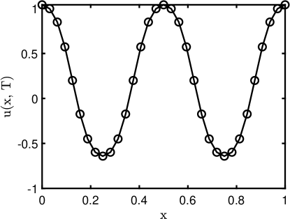
Figure 1: Advection equation: $\medcircle,-$ denote SASK and the reference, respectively.

5.1.2 Heat equation

The following is a heat diffusion equation. Here, we also incorporate an initial condition:

$$\dfrac{\partial u}{\partial t}=\dfrac{1}{80\pi^{2}}\dfrac{\partial^{2}u}{\partial x^{2}},\quad x\in[0,1],$$ (25)

$$u(x,0)=\sin(4\pi x).$$

This equation has a closed-form solution $u(x,t)=\sin(4\pi x)e^{-0.2t}$. Specifying parameters $m=32,n=10,r=0.1,\gamma=0.2$, we obtain SASK numerical solutions at $T=10$. The comparison between the exact solutions with the numerical solutions is exhibited in Figure 2. In particular, $e_{L_{2}}=8.69\times 10^{-16}$ and $e_{L_{\infty}}=9.08\times 10^{-15}$. As in the advection equation case, the semi-discrete form is a linear ODE system, and we observed that SASK achieved high accuracy even when $n=1$, because the adaptivity was barely triggered due to the linearity of the dynamics.

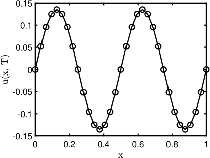
Figure 2: Heat equation: $\medcircle,-$ denote SASK and the reference, respectively.

5.1.3 Korteweg-de Vries equation

The next example is the Korteweg-de Vries (KdV) equation with a solitary wave solution:

$$\dfrac{\partial u}{\partial t}+\beta u\dfrac{\partial u}{\partial x}+\mu\dfrac{\partial^{3}u}{\partial x^{3}}=0,\quad x\in\mathbb{R},$$ (26)

$$u(x,0)=\dfrac{3c}{\beta}sech^{2}\left(\dfrac{1}{2}\sqrt{c/\mu}\,x\right).$$

The closed-form solution is $u(x,t)=\dfrac{3c}{\beta}sech^{2}\left(\dfrac{1}{2}\sqrt{c/\mu}(x-ct)\right)$. Here, $\beta,\mu,c$ are constants, and $c$ is the wave speed. In this test, we set $c=0.5,\beta=3,\mu=9$. In general, the solution decays to zeros for $|x|>>1$. Therefore, numerically we solve this equation in a finite domain $[-p,p]$ with a periodic boundary condition. In this example we set $p=45$. Furthermore, as shown in [6, 25], a change of variable step $(x\rightarrow\pi x/p+\pi)$ transforms the solution interval from $[-p,p]$ to $[0,2\pi]$. Consequently, $\beta$ and $\mu$ in Equation 26 are replaced by $\tilde{\beta}=\frac{\beta\pi}{p}$ and $\tilde{\mu}=\frac{\mu\pi^{3}}{p^{3}}$, respectively. For the spatial discretization, we set $m=100$ since the behavior of the KdV equation requires finer spatial grids. The parameter associated with SASK are $n=100,r=0.1,\gamma=0.8$. SASK computed the solutions at $T=10$, giving the illustration in Figure 3. Finally, the errors are $e_{L_{2}}=1.60\times 10^{-4}$ and $e_{L_{\infty}}=1.40\times 10^{-4}$.

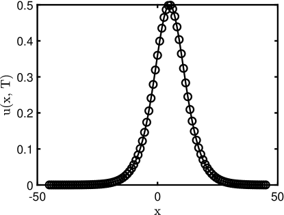
Figure 3: KdV equation: $\medcircle,-$ denote SASK and the reference, respectively.

5.1.4 Burgers equation

The last example is a viscous Burgers equation with an initial condition is considered:

$$\dfrac{\partial u}{\partial t}+u\dfrac{\partial u}{\partial x}=\nu\dfrac{\partial^{2}u}{\partial x^{2}},\quad x\in[0,1],$$ (27)

$$u(x,0)=0.2+\sin(2\pi x).$$

The advection term $uu_{x}$ is treated in the conservation form, i.e., $\frac{1}{2}(u^{2})_{x}$. Particularly, the reference solution is obtained by the high-order spectral method. For this example, the degree of freedom in space is $m=64$, and SASK admits the parameters $n=50,r=0.1,\gamma=1$. With $\nu=0.005$ and $T=1$, SASK yields $e_{L_{2}}=8.85\times 10^{-4}$ and $e_{L_{\infty}}=1.80\times 10^{-3}$. The result is presented in Figure 4, which indicates that the solution is accurate before the discontinuity is fully developed. Additionally, we will observe the Gibbs phenomenon near the discontinuity, if we keep increasing $T$.

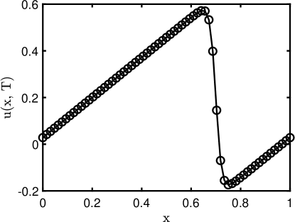
Figure 4: Burgers equation: $\medcircle,-$ denote SASK and the reference, respectively.

5.2 Efficiency comparison

To demonstrate the efficiency of SASK compared with RK4, we target on the running time of the two methods based on the PDEs. Particularly, RK4 leverages the Fourier differentiation matrix to solve the semi-discrete form after spatial discretization. The parameters used in the four PDEs are specified as follows:

1. Adevection equation: $m=32,T=100,n=1,r=1,\gamma=0.2$;

2. Heat equation: $m=32,T=10,n=10,r=0.1,\gamma=0.5$;

3. KdV equation: $c=0.5,\beta=3,\mu=9,p=45,m=100,T=10,n=100,r=0.1,\gamma=0.8$;

4. Burgers equation: $\nu=0.005,m=64,T=1,n=100,r=0.1,\gamma=1$.

We summarize the results in Table 1. The first row of each PDE is the running time, while the second and the third are the relative $L_{2}$ error and the $L_{\infty}$ error. For the advection equation and the heat equation, the dynamics of their semi-discrete form are linear so SASK needs only a small number of check points and updates to be accurate. This results in SASK’s higher computational efficiency than RK4’s. In contrast, Burgers equation and KdV equation require more updates, so it takes SASK more computations to preserve accuracy. For the KdV equation, SASK still outperforms RK4, but for the Burgers equation, SASK needs around 10 times the time of RK4 to reach a comparable level of accuracy. This is because for the Burgers equation, SASK requires more adaptivity steps to track the evolution of the states, which is probably due to the regularity of the system itself. Hence, SASK gains an edge over RK4 when $T$ is large, or when the dynamics are not so nonlinear that it allows for a small number of updates.

Table 1: Performance comparison between SASK and RK4 on PDEs: $L_{2}$ denotes the relative error computed with $2$-norm, while $L_{\infty}$ denotes the error computed with $\infty$-norm. The normalized time is reported.

		SASK	RK4
Advection Equation	time	1.00	21.47
	$L_{2}$	2.80e-11	1.49e-07
	$L_{\infty}$	3.02e-11	1.78e-07
Heat Equation	time	1.00	13.28
	$L_{2}$	7.57e-15	9.24e-15
	$L_{\infty}$	1.19e-15	1.85e-15
KdV Equation	time	1.00	3.97
	$L_{2}$	1.5972e-04	1.5968e-04
	$L_{\infty}$	1.4030e-04	1.4090e-04
Burgers Equation	time	1.00	0.1
	$L_{2}$	4.94e-04	4.88e-04
	$L_{\infty}$	6.13e-04	4.96e-04

6 Conclusion and Discussion

In this work, we propose the sparse-grid-based ASK method to solve autonomous dynamical systems. Leveraging the sparse grid method, SASK is an efficient extension of the ASK for high-dimensional ODE systems. Also, we demonstrate SASK’s potential of solving PDEs efficiently by solving semi-discrete systems. In particular, our numerical results demonstrate that if the semi-discrete form is a linear function of the discretized solution of the PDE, SASK is very accurate and much more efficient than conventional ODE-solver-based methods because SASK is a high order method for solving dynamical systems. Furthermore, by selecting the adaptivity criteria carefully, SASK can solve highly nonlinear PDEs like the KdV equation and deal with large total variation in the solution like the Burgers’ equation. Moreover, we only used level-1 sparse grid method in SASK to obtain good results in the illustrative examples. In our future work, we will further investigate the selection of adaptivity parameters and the requirement on the accuracy level of the sparse grid method. Finally, it is possible to use other sampling strategies combined with different basis functions like radial basis functions or activation functions used in neural networks to further enhance the accuracy and efficiency of ASK for some high-dimensional problems.

Appendix A Sparse grid illustration

Figure 5 is an illustration of sparse grids and their full grid counterparts.

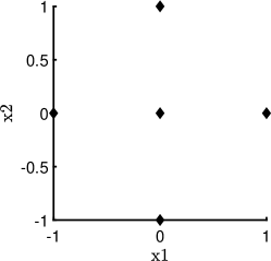
(a)

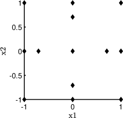
(b)

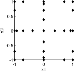
(c)

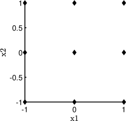
(d)

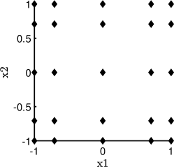
(e)

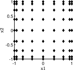
(f)

Figure 5: Sparse grid (first row) - full grid (second row): $n$ denotes the number of points in each dimension.

To give a brief view of the growth in the grid size, Table 2 shows that the full grid grows much faster than the sparse grid. Notably, the sparse grid grows surprisingly slow in practice, although its theoretical order is exponential in $d$.

Table 2: Grid Growth: $n$ denotes the number of points in each dimension.

$d$	$\kappa=1$	$n=3$	$\kappa=2$	$n=5$	$\kappa=3$	$n=9$
2	5	9	13	25	29	81
3	7	27	25	125	69	729
4	9	81	41	625	137	6561
5	11	243	61	3125	241	59049

References

- [1] Travis Askham and J Nathan Kutz. Variable projection methods for an optimized dynamic mode decomposition. SIAM Journal on Applied Dynamical Systems, 17(1):380–416, 2018.
- [2] Steven L Brunton, Marko Budišić, Eurika Kaiser, and J Nathan Kutz. Modern Koopman theory for dynamical systems. arXiv preprint arXiv:2102.12086, 2021.
- [3] Hans-Joachim Bungartz and Michael Griebel. Sparse grids. Acta numerica, 13:147–269, 2004.
- [4] Akshunna S Dogra and William Redman. Optimizing neural networks via Koopman operator theory. Advances in Neural Information Processing Systems, 33:2087–2097, 2020.
- [5] Bengt Fornberg. A practical guide to pseudospectral methods. Number 1. Cambridge university press, 1998.
- [6] Bengt Fornberg and Gerald Beresford Whitham. A numerical and theoretical study of certain nonlinear wave phenomena. Philosophical Transactions of the Royal Society of London. Series A, Mathematical and Physical Sciences, 289(1361):373–404, 1978.
- [7] Thomas Gerstner and Michael Griebel. Numerical integration using sparse grids. Numerical algorithms, 18(3):209–232, 1998.
- [8] Michael Griebel, Michael Schneider, and Christoph Zenger. A combination technique for the solution of sparse grid problems. 1990.
- [9] Jan S Hesthaven, Sigal Gottlieb, and David Gottlieb. Spectral methods for time-dependent problems, volume 21. Cambridge University Press, 2007.
- [10] Kenneth L Judd, Lilia Maliar, Serguei Maliar, and Rafael Valero. Smolyak method for solving dynamic economic models: Lagrange interpolation, anisotropic grid and adaptive domain. Journal of Economic Dynamics and Control, 44:92–123, 2014.
- [11] Bernard O Koopman. Hamiltonian systems and transformation in Hilbert space. Proceedings of the National Academy of Sciences of the United States of America, 17(5):315, 1931.
- [12] Milan Korda, Mihai Putinar, and Igor Mezić. Data-driven spectral analysis of the Koopman operator. Applied and Computational Harmonic Analysis, 48(2):599–629, 2020.
- [13] J Nathan Kutz, Steven L Brunton, Bingni W Brunton, and Joshua L Proctor. Dynamic mode decomposition: data-driven modeling of complex systems. SIAM, 2016.
- [14] J Nathan Kutz, Xing Fu, and Steven L Brunton. Multiresolution dynamic mode decomposition. SIAM Journal on Applied Dynamical Systems, 15(2):713–735, 2016.
- [15] Bian Li, Yi-An Ma, J Nathan Kutz, and Xiu Yang. The adaptive spectral koopman method for dynamical systems. arXiv preprint arXiv:2202.09501, 2022.
- [16] Igor Mezić. Spectral properties of dynamical systems, model reduction and decompositions. Nonlinear Dynamics, 41(1):309–325, 2005.
- [17] Igor Mezić. Spectrum of the Koopman operator, spectral expansions in functional spaces, and state-space geometry. Journal of Nonlinear Science, 30(5):2091–2145, 2020.
- [18] Hiroya Nakao and Igor Mezić. Spectral analysis of the Koopman operator for partial differential equations. Chaos: An Interdisciplinary Journal of Nonlinear Science, 30(11):113131, 2020.
- [19] J Nathan Kutz, Joshua L Proctor, and Steven L Brunton. Applied Koopman theory for partial differential equations and data-driven modeling of spatio-temporal systems. Complexity, 2018, 2018.
- [20] Marcos Netto and Lamine Mili. A robust data-driven Koopman kalman filter for power systems dynamic state estimation. IEEE Transactions on Power Systems, 33(6):7228–7237, 2018.
- [21] Jacob Page and Rich R Kerswell. Koopman analysis of Burgers equation. Physical Review Fluids, 3(7):071901, 2018.
- [22] Joshua L Proctor, Steven L Brunton, and J Nathan Kutz. Dynamic mode decomposition with control. SIAM Journal on Applied Dynamical Systems, 15(1):142–161, 2016.
- [23] Clarence W Rowley, Igor Mezić, Shervin Bagheri, Philipp Schlatter, and Dan S Henningson. Spectral analysis of nonlinear flows. Journal of fluid mechanics, 641:115–127, 2009.
- [24] Peter J Schmid. Dynamic mode decomposition of numerical and experimental data. Journal of fluid mechanics, 656:5–28, 2010.
- [25] Jie Shen and Tao Tang. Spectral and high-order methods with applications. Science Press Beijing, 2006.
- [26] Sergei Abramovich Smolyak. Quadrature and interpolation formulas for tensor products of certain classes of functions. In Doklady Akademii Nauk, volume 148, pages 1042–1045. Russian Academy of Sciences, 1963.
- [27] Amit Surana and Andrzej Banaszuk. Linear observer synthesis for nonlinear systems using Koopman operator framework. IFAC-PapersOnLine, 49(18):716–723, 2016.
- [28] Lloyd N Trefethen. Spectral methods in MATLAB. SIAM, 2000.
- [29] Jonathan H Tu, Clarence W Rowley, Dirk M Luchtenburg, Steven L Brunton, and J Nathan Kutz. On dynamic mode decomposition: Theory and applications. Journal of Computational Dynamics, 1(2):391–421, 2014.
- [30] Matthew O Williams, Ioannis G Kevrekidis, and Clarence W Rowley. A data–driven approximation of the Koopman operator: Extending dynamic mode decomposition. Journal of Nonlinear Science, 25(6):1307–1346, 2015.
- [31] Dan Wilson and Jeff Moehlis. Isostable reduction with applications to time-dependent partial differential equations. Physical Review E, 94(1):012211, 2016.
- [32] Christoph Zenger and W Hackbusch. Sparse grids. In Proceedings of the Research Workshop of the Israel Science Foundation on Multiscale Phenomenon, Modelling and Computation, page 86, 1991.