Sensitivity of Neutron Star Observations to Three-nucleon Forces

Abstract

Astrophysical observations of neutron stars have been widely used to infer the properties of the nuclear matter equation of state. Beside being a source of information on average properties of dense matter, the data provided by electromagnetic and gravitational wave (GW) facilities are reaching the accuracy needed to constrain, for the first time, the underlying nuclear dynamics. In this work we assess the sensitivity of current and future neutron star observations to directly infer the strength of repulsive three-nucleon forces, which are key to determine the stiffness of the equation of state. Using a Bayesian approach we focus on the constraints that can be derived on three-body interactions from binary neutron star mergers observed by second and third-generation of gravitational wave interferometers. We consider both single and multiple observations. For current detectors at design sensitivity the analysis suggests that only low mass systems, with large signal-to-noise ratios (SNR), allow to reliably constrain the three-body forces. However, our results show that a single observation with a third-generation interferometer, such as the Einstein Telescope or Cosmic Explorer, will constrain the strength of the repulsive three-nucleon potential with exquisite accuracy, turning third-generation GW detectors into new laboratories to investigate the properties of nucleon interactions.

I Introduction

Lying at the interface between electromagnetic (EM) observatories, gravitational wave interferometers, and Earth based laboratories, multi-messenger astrophysics has the potential to shape a novel view of both structure and dynamics of dense nuclear matter. Mass-radius measurements of rotating pulsars are rapidly improving thanks to the information provided by the NASA satellite NICER [1, 2, 3, 4, 5, 6], which has recently targeted the most massive neutron star (NS) known so far. Remarkably, NICER observations of PSR J0030+0451 and PSR J0740+662—the inferred masses of which are $M={1.34}_{-0.15}^{+0.16}$ ($M=1.44^{+0.15}_{-0.14}M_{\odot}$) and $M={2.072}_{-0.066}^{+0.067}\ M_{\odot}$, respectively—yield comparable values of the stellar radius, pointing to a stiff nuclear matter equation of state (EOS) up to densities around four times nuclear density. On the other hand, constraints inferred from binary NS mergers detected by the LIGO/Virgo Collaboration, and in particular from the landmark discovery of GW170817, [7, 8, 9, 9], have already ruled out some of the stiffest EOSs, which predict large tidal deformabilities, hinting instead to a softer matter content [10, 11, 12, 13, 14, 15]. In addition, astrophysical data are being complemented by the information coming from terrestrial experiments, such as heavy-ion collisions or the recent measurement of the neutron skin thickness of lead, performed at Jefferson Lab by the PREX-II Collaboration [16, 17, 18, 19, 20, 21, 22, 23].

Posterior distributions inferred from space- and ground-based facilities have been widely exploited in a variety of multi-messenger analyses, aimed at constraining models of the EOS or specific properties of neutron star matter. Examples of this approach include reconstruction of the EOS within both phenomenological and non-parametric frameworks, calculations based on microscopic models, and analyses focused on features such as the occurrence of phase transitions, or the behavior of the symmetry energy above nuclear density [24, 25, 26, 27, 28, 29, 30, 31, 32, 33, 34, 35, 35, 36, 37, 38, 39, 40, 41, 42, 43, 44, 45, 46, 47, 48, 49, 50]; for recent reviews, see also Refs. [51, 52] and references therein.

Recently, some of the authors of this article have proposed a novel approach, aimed at pushing the analyses based on multimessenger astrophysical information to a deeper level [53]. They argued that the accuracy of the currently available data—as well as that expected to be achieved by operating the existing detectors at design sensitivity—offer an unprecedented opportunity to constrain the microscopic models of nuclear dynamics at supranuclear density. The results reported in Ref. [53] show that the data set comprising the GW observation of the binary NS event GW170817, the spectroscopic observation of the millisecond pulsars PSR J0030+0451 performed by the NICER satellite, and the high-precision measurement of the radio pulsars timing of the binary PSR J0740+6620, providing information on the maximum NS mass, can, in fact, be exploited to infer quantitative insight on the strength of repulsive three-nucleon interactions in dense matter.

Unlike the nucleon-nucleon potential, the models of irreducible three-nucleon interactions are totally unconstrained beyond nuclear density. In most models, e.g. the Urbana IX potential employed to derive the EOS of Akmal, Pandharipande and Ravenhall (APR) [54], the strength of the isoscalar repulsive term—which plays a pivotal role in determining the stiffness of the nuclear matter EOS in the region relevant to neutron stars—is determined in such a way as to reproduce the empirical equilibrium density of isospin-symmetric matter [55, 56]. In this context, the availability of additional information constraining the three-nucleon potential at larger density would be a major breakthrough.

The present work can be seen as a complementary follow up to the pioneering study of Ref. [53]. The analysis is first extended to consider a near-future scenario, using current interferometers at design sensitivity and stacking multiple binary NS observations characterised by different masses and distances. In addition, we apply, for the first time, the Bayesian approach to gauge the sensitivity of the Einstein Telescope (ET), a proposed third-generation ground-based GW observatory [57, 58, 59]

The body of the article is structured as follows. In Sect. II we outline the dynamical model underlying our study, as well as the simple parametrisation adopted to characterise the strength of the repulsive component of the three-nucleon potential. The datasets considered in the analysis and the details of numerical simulations are described in Sections III.1 and III.2, respectively, while the results are reported and discussed in Sect. IV. Finally, a summary of our findings and the prospects for future developments can be found in in Sect. V.

II Modelling Nuclear Dynamics Beyond Nuclear Density

The EOSs considered in our study have been derived using the formalism of non-relativistic nuclear many-body theory (NMBT). Within this framework, nuclear matter is pictured as a uniform system of point like nucleons, the dynamics of which is completely determined by the Hamiltonian

$${H}=\sum_{i}\frac{p_{i}^{2}}{2m}+\sum_{i<j}v_{ij}+\sum_{i<j<k}V_{ijk}\ ,$$ (1)

where $m$ and $p_{i}$ denote the mass and momentum of the $i$-th nucleon, respectively. Interactions between matter constituents are driven by the nucleon-nucleon (NN) potential $v_{ij}$—providing an accurate description of the two-nucleon system in both bound and scattering states—supplemented by the three-nucleon (NNN) potential $V_{ijk}$, whose inclusion is needed to implicitly take into account the occurrence of processes involving the internal structure of the nucleon. As a consequence, the role of NNN interactions is expected to become more and more important with increasing density.

Starting from Eq. (1), a number of different EOSs have been obtained using both different Hamiltonian models and different many-body techniques to calculate the ground state energy of nuclear matter as a function of baryon density. Purely phenomenological Hamiltonians, fitted to the properties of two- and three-nucleon systems, have been shown to provide a remarkably accurate account of the energies of the ground and low-lying excited states of nuclei with mass number $A\leq 12$, as well as of their radii [60]. In addition, they allow to reproduce the empirical value of the equilibrium density of isospin-symmetric matter (SNM); see, e.g., Ref. [54]

Over the past two decades, a great deal of attention has been given to a novel generation of nuclear Hamiltonians, derived using the formalism of Chiral Effective Field Theory ($\chi$EFT). Within $\chi$EFT, the nuclear potentials are obtained from effective Lagrangians comprising pion and nucleon degrees of freedom, constrained by the chiral symmetry of strong interactions. The main advantage of this approach is the capability to determine two- and many-nucleon potentials in a fully consistent fashion. However, being based on a low momentum expansion its applicability is inherently limited to densities $\lesssim 2\varrho_{0}$, with $\varrho_{0}=0.16\ {\rm fm}^{-3}$ being the saturation density of SNM [61, 62].

In this study, we have considered purely phenomenological Hamiltonians, which are expected to be best suited to describe the properties of nuclear matter in the density region extending up to $\sim 5\varrho_{0}$, relevant to NS applications. The reference line of our analysis is the Hamiltonian comprising the Argonne $v_{18}$ NN potential [63] (AV18) and the Urbana IX NNN potential [56, 55] (UIX), which has been employed to obtain the APR EOS [64, 54].

The AV18 potential is written as a sum of eighteen terms, needed to describe the complex operator structure of nuclear forces. It provides an accurate fit of the NN scattering phase-shifts for laboratory-frame energies up to $\sim 600$ MeV, a value typical of NN collisions in strongly degenerate matter at density $\varrho\sim 4\varrho_{0}$ [61]. A comparison with the central densities obtained from the solution of the Tolman-Oppenheimer-Volkoff equations [65, 66] with the APR EOS [67] suggests that this phenomenological potential is adequate to describe NSs having masses as large as $\sim 2.1$ M_⊙.

The UIX model of the NNN interaction is written as the sum of an attractive potential first derived by Fujita and Miyazawa [68]—describing two-pion exchange NNN processes with excitation of a $\Delta$-resonance in the intermediate state—and a phenomenological repulsive potential; the resulting expression is

$$V_{ijk}=V_{ijk}^{2\pi}+V_{ijk}^{R}\ .$$ (2)

The strength of the two-pion exchange contribution is adjusted to reproduce the observed ground state energies of [3][]H and [4][]He, obtained from accurate Monte Carlo calculations [55], whereas that of the isoscalar repulsive term is fixed to obtain the empirical saturation density of SNM—inferred from nuclear data—from variational calculations carried out using advanced many-body techniques [56].

It should be kept in mind that the repulsive term $V_{ijk}^{R}$ implicitly takes into account relativistic corrections to the phenomenological two-nucleon potential $v_{ij}$, which is determined by fitting NN scattering data in the center-of-mass reference frame. In the presence of the nuclear medium, however, the center of mass of the interacting nucleon pair is not at rest, and $v_{ij}$ must be boosted to take into account its motion [69].

The authors of Ref. [54] have modified the free-space AV18 potential to include the boost correction $\delta v$, whose effect is an enhancement of the repulsive contribution to the potential energy. As a consequence, using the boosted AV18 potential in calculations of nuclear matter energy entails the introduction of a modified NNN potential, referred to as UIX^∗, which turns out to be considerably softer than the UIX. The impact of relativistic corrections to the nuclear Hamiltonian on the description of NS properties has been recently discussed in Ref. [67].

The potentials describing NNN interactions are only determined by nuclear phenomenology reflecting nucleon interactions at SNM saturation density. On the other hand, they are totally unconstrained in the high-density regime relevant to NSs, in which their contribution is known to become dominant.

Motivated by the above consideration, in this work we extend the study of Ref. [53], whose authors have explored the possibility of inferring the strength of the repulsive term of the UIX^∗ potential from data collected by multimessenger astrophysical observations, which carry information on nuclear dynamics at supranuclear denisity. Note that to pin down the dynamics of NNN interactions it is essential that the analysis be carried out using the the boost corrected NN potential.

Our study is based on the use of a set of Hamiltonians, obtained from the AV18 + $\delta v$ + UIX^∗ model performing the replacement

$$\langle V_{ijk}^{R}\rangle\rightarrow\alpha\langle V_{ijk}^{R}\rangle\ .$$ (3)

The energy-density of nuclear matter at arbitrary baryon density $\varrho$ and proton fraction $x_{p}$ has been obtained generalising the parametrisation employed in Ref.[54], that can be written in the form

$$\epsilon(\varrho,x_{p}) =\left[\frac{\hbar^{2}}{2m}+f(\varrho,x_{p})\right]\tau_{p}$$ (4)

$$+\left[\frac{\hbar^{2}}{2m}+f(\varrho,1-x_{p})\right]\tau_{n}+g(\varrho,x_{p}),$$

where

$$g(\rho,x_{p})=g(\rho,1/2)+\left[g(\rho,0)-g(\varrho,1/2)\right](1-2x_{p})^{2}.$$ (5)

The explicit expressions of the functions appearing in Eqs. (4) and (5) can be found in the Appendix. They involve a set of parameters which were determined by fitting the energy per nucleon of SNM and pure neutron matter (PNM) computed within the FHNC/SOC variational approach [70] using the AV18+ $\delta v$ + UIX^∗ Hamiltonian.

The first two terms of Eq. (4) correspond to the proton and neutron kinetic energy, respectively, whereas the function $g(\rho,x_{p})$ describes the contribution arising from interactions. The assumption of quadratic dependence of the interaction energy on the neutron excess $\delta=1-2x_{p}$ is routinely employed in the literature to obtain the EOS of $\beta$-stable matter from those of SNM and PNM, and has been shown to be remarkably accurate over a broad range of values of the proton fraction $x_{p}$; see, e.g. Ref. [71].

Implementing the substitution of Eq. (3) is equivalent to adding a term $(\alpha-1)V^{R}$ at first order in perturbation theory. The corresponding change of energy density turns out to be

$$g(\varrho,x_{p})\rightarrow g(\varrho,x_{p},\alpha)=g(\varrho,x_{p})+\delta g(\varrho,x_{p},\alpha),$$ (6)

with

$$\delta g(\varrho,x_{p},\alpha) =\delta g(\varrho,1/2,\alpha)\left[1-(1-2x_{p})^{2}\right]$$ (7)

$$+\delta g(\varrho,0,\alpha)(1-2x_{p})^{2}\ .$$

The functions $\delta g$ can be readily expressed in terms of expectation values of $V^{R}$ in the nuclear matter ground state using

$$\delta g(\varrho,1/2,\alpha)=\frac{\varrho}{A}(\alpha-1)\langle V^{R}_{ijk}\rangle_{\textnormal{SNM}}\ ,$$ (8)

$$\delta g(\varrho,0,\alpha)=\frac{\varrho}{A}(\alpha-1)\langle V^{R}_{ijk}\rangle_{\textnormal{PNM}}\ .$$ (9)

Tabulated values of $\langle V_{ijk}^{R}\rangle$ as a function of density can be found in Ref. [54]. In our analysis, we have employed a polynomial fit including powers up to $\varrho^{3}$

$$\langle V^{R}_{ijk}\rangle=a_{0}+a_{1}\,\varrho+a_{2}\,\varrho^{2}+a_{3}\,\varrho^{3}\ ,$$ (10)

which turned out to be very accurate. The values of the parameters $a_{i}$ are reported in Table 1.

Table 1: Values of the parameters appearing in Eq. (10), corresponding to $\langle V^{R}_{ijk}\rangle$ in MeV and $\varrho$ in fm^-3.

	$a_{0}$	$a_{1}$	$a_{2}$	$a_{3}$
	$[{\rm MeV}]$	$[{\rm MeV}\ {\rm fm}^{3}]$	$[{\rm MeV}\ {\rm fm}^{6}]$	$[{\rm MeV}\ {\rm fm}^{9}]$
SNM	0.754	-16.769	214.164	77.422
PNM	0.949	-27.403	241.407	64.995

Using the analytic expression of the energy density of nuclear matter at arbitrary proton fraction, composition and energy density of $\beta$-stable matter can be easily determined, by minimising with respect to $x_{p}$, with the additional constraints of conservation of baryon number and charge neutrality. Finally, the matter pressure $P$, derived from standard thermodynamic relations, is used to obtain the EOS $P(\epsilon)$.

It has to be kept in mind that changing the strength of $V^{R}_{ijk}$ affects the value of the nuclear saturation density predicted by the AV18 + $\delta v$ + UIX^∗ Hamiltonian. For this reason, we have limited the acceptable range of $\alpha$ to the interval $[0.7,2.0]$. Within this range, the departure from the empirical value of $\varrho_{0}$ turns out to be $\sim 15\%$ at most, and the corresponding change of the energy per particle never exceeds 3%.

Moreover, because the contribution of the repulsive NNN potential becomes large at supranuclear densities, the modification of its strength $\alpha$ marginally affect the ground-state energy of atomic nuclei. Using the results reported in Ref. [72], obtained from accurate Quantum Monte Carlo calculations, we have found that changing $\alpha$ from 1 to 1.3 results in a change of $4\%$ and $6\%$ of the ground state energies of [4][]He and [12][]C, respectively. These discrepancies appear to be fully acceptable in the context of our exploratory study.

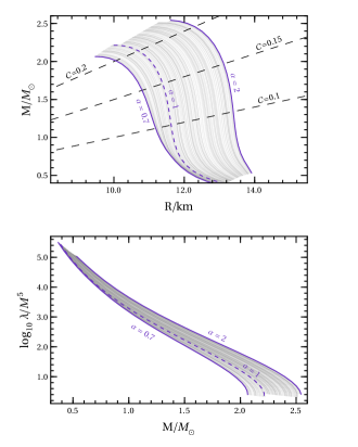
Figure 1: (Top) Representative ensemble of the mass-radius profiles for the family of EOS considered in this work. Each gray curve corresponds to a specific value of $\alpha$ drawn between the solid violet lines which refer to the lower and upper bounds of $\alpha$ assumed in the analysis, i.e. $\alpha=0.7$ and $\alpha=2$, respectively. The dashed curve identifies the baseline APR model with $\alpha=1$. We also show lines of constant compactness ${\cal C}=M/R$. (Bottom) Same as top panel but for the dimensionless tidal deformability $\lambda/M^{5}$ as a function of the NS mass.

III Methods and observations

We consider a family of EOS for which the observables of a neutron star (mass, radius and tidal deformability) depend uniquely on the three-body coefficient $\alpha$ and on the central pressure $p_{c}$:

$$\{\alpha,p_{c}\}\rightarrow\{M,R,\lambda\}\ .$$ (11)

Figure 1 shows the stable stellar configurations in the mass-radius plane and the mass-tidal deformability plane. Given a set $O_{i=1,\dots,n}$ of observations, we infer $\{\alpha,p_{c}^{(1)}\dots p_{c}^{(m)}\}$ using a hierarchical Bayesian approach,

$$\mathcal{P}(\alpha,\vec{p}_{c}|\vec{O})\propto\mathcal{P}_{0}(\alpha,\vec{p}_{c})\prod_{i=1}^{m}\mathcal{L}(O_{i}|\theta_{i})$$ (12)

where $\vec{p}_{c}=\{p_{c}^{(1)}\dots p_{c}^{(m)}\}$, $\mathcal{L}(O_{i}|\theta_{i})$ is the likelihood of the $i$-th event (see Sec. III.1 below) and $\theta_{i}$ denotes the set of relevant NS observables — mass and radius for pulsars, symmetric mass ratio and effective tidal deformability for GW observations — evaluated at $\{\alpha,p_{c}^{(i)}\}$ via (11). We assume that the priors on $\alpha$ and on each central pressure in Eq. (12) are uncorrelated.

The posteriors in Eq. (12) are sampled using the emcee with stretch move [73]. For each observation we run 100 walkers of $10^{6}$ samples with a thinning factor of $0.02$. The final distribution for $\alpha$ is obtained by marginalizing over the central pressures $\vec{p}_{c}$. When presenting results, we quote the median alongside the bounds of the $90\%$ symmetric posterior density intervals.

We sample the central pressures of each star uniformly in log-space between $\ln_{10}p_{c}^{\textnormal{min}}(\alpha)\simeq 34.58$, where $p_{c}$ is expressed in $\mbox{dyne}/\mbox{cm}^{2}$, and $\ln_{10}p_{c}^{\textnormal{max}}(\alpha)$, where $p_{c}^{\textnormal{max}}$ corresponds to the central pressure of the heaviest stable configuration for each EOS specified by $\alpha$. The lower value $p_{c}^{\textnormal{min}}$ is chosen such that the nuclear model supports masses larger than $0.8M_{\odot}$. The values of $\alpha$ are drawn from a uniform distribution in the range $[0.7,2]$. We also impose a causality constraint, requiring that the speed of sound $c_{s}=\sqrt{dp/d\epsilon}$ is subluminal at the center of each NS.

III.1 Astrophysical datasets

We consider three real datasets corresponding to (i) the binary coalescence GW170817, (ii) the millisecond pulsar PSR J0030+0451 and (iii) the heaviest NS observed so far PSR J0740+6620. Dataset (iii) provides and update w.r.t. [53], in which PSR J0740+6620 was included only through the measurement of its mass, while here we also include the radius. We briefly summarize here the basic properties of each dataset and the corresponding likelihood functions that enter Eq. (12).

(i) — GW170817 is the first binary neutron star system observed by LIGO and Virgo. Under a low spin prior, the LVC analysis constrained the source component masses $(m_{1},m_{2})$ between $\sim 1.16M_{\odot}$ and $\sim 1.6M_{\odot}$. GW170817 provided the first evidence that GW signals from coalescing systems are sensitive to matter effects induced by the NS structure, yielding a measurement for the effective tidal parameter

$$\tilde{{\Lambda}}=\frac{16}{13}\left[\frac{(m_{1}+12m_{2})m_{1}^{4}\Lambda_{1}}{(m_{1}+m_{2})^{5}}\ +\ 1\leftrightarrow 2\right]$$ (13)

of $\tilde{\Lambda}=300^{+420}_{-230}$ within $90\%$ of the highest posterior density interval, with $\Lambda_{1,2}=\lambda_{1,2}/m_{1,2}^{5}$ being the NS individual, dimensionless, tidal deformabilities [7].

We construct the likelihood $\mathcal{L}(O_{\rm GW170817}|\eta,\tilde{\Lambda})$ from the joint posterior ${\cal P}({\cal M},\eta,\tilde{{\Lambda}}|O_{\textnormal{GW170817}})$ for $\tilde{\Lambda}$, the chirp mass ${\cal M}=(m_{1}m_{2})^{3/5}/(m_{1}+m_{2})^{1/5}$, and the symmetric mass ratio $\eta=m_{1}m_{2}/(m_{1}+m_{2})^{5}$. The calculation can be simplified by the fact that the chirp mass in the source frame is measured with $\sim 0.1\%$ precision, which allows to fix it to its median value $\mathcal{M}_{\star}=1.186~{}M_{\odot}$ and restrict to the conditional probability $\mathcal{P}(\eta,\tilde{\Lambda}|\mathcal{M}_{\star},O_{\rm GW170817})$. Moreover, as shown in [33], the latter can be replaced by the marginalized posterior ${\cal P}(\eta,\tilde{\Lambda}|O_{\textnormal{GW170817}})$ to very good accuracy. This choice reduces the number of parameters to be sampled, since the central pressure $p_{c}^{(2)}$ of the secondary component is uniquely determined by $\{\mathcal{M}_{\star},p_{c}^{(1)}\}$ and $\alpha$ , and similarly for the individual masses $m_{1,2}$ and tidal deformabilities $\Lambda_{1,2}$. The likelihood function is then obtained by re-weighting the posterior by the joint prior on $\eta$ and $\tilde{\Lambda}$ as derived from [7],

$${\cal L}(O_{\textnormal{GW170817}}|\eta,\tilde{\Lambda})=\frac{{\cal P}(\eta,\tilde{\Lambda}|O_{\textnormal{GW170817}})}{{\cal P}_{0}(\eta,\tilde{\Lambda})}\ .$$ (14)

Note that, although $p_{c}^{(2)}$ is not independently sampled, we still require it to lie within its prior support.

(ii) — For the millisecond pulsar PSR J0030+0451 we use the joint mass-radius posterior ${\cal P}(M,R|O_{J0030})$ inferred by the NICER collaboration, which has carried out two independent studies of the stellar spectroscopic observations, obtaining consistent results. The mass-radius constraints provided by the two collaborations led to $M=1.34^{+0.15}_{-0.16}M_{\odot}$ and $R=12.71^{+1.14}_{-1.19}$km [3], and $M=1.44^{+0.15}_{-0.14}M_{\odot}$ and $R=13.02^{+1.24}_{-1.06}$km [4] respectively ($68\%$ credibility). Here we use the data publicly available in [74], for which the likelihood can be derived straightforwardly from ${\cal P}(M,R|O_{J0030})$ because the joint prior on $\{M,R\}$ is flat,

$$\mathcal{L}(O_{\rm J0030}|M,R)\propto\mathcal{P}(M,R|O_{\rm J0030})\,.$$ (15)

(iii) — PSR J0740+6620 [5, 6] is the most massive pulsar discovered so far. Previous observations of this source constrained its mass to $M=2.08^{+0.072}_{-0.069}M_{\odot}$ (68.3% credibility) [2]. This measurement, combined with data obtained from the XMM Newton European Photon Imaging Camera to improve the NICER background, was used in [5, 75] and [6, 76] to infer the pulsar radius, with the two teams obtaining $R=12.39^{+1.30}_{-0.98}$km and $R=13.7^{+2.62}_{-1.50}$km [6] respectively (68% credibility). Here we use the data in [77], for which the likelihood can be immediately inferred from the posterior due to uniform priors,

$$\mathcal{L}(O_{\rm J0740}|M,R)\propto\mathcal{P}(M,R|O_{\rm J0740})\,.$$ (16)

III.2 Simulations for 2G and 3G detectors

We simulate 30 binary neutron star events for two choices of the three-body strength, $\alpha=1$ and $\alpha=1.3$, either for a network (HLV) composed by the LIGO Hanford, LIGO Livingston, and Virgo detectors at design sensitivity [79], or for the future third-generation interferometer Einstein Telescope in its ET-D configuration [58]. We inject 64-second long waveforms into a zero-noise configuration as described in [80], with sky location and inclination uniformily distributed over the sky. Posterior parameters are recovered using the bilby software [81, 82] for GW injections and parameter estimation. For both injection and recovery, we model binary neutron star signals with the IMRPhenomPv2_NRTidal waveform template [83, 84]. Injected binaries are nonspinning, while component spins are recovered imposing a low-spin prior $\chi_{1,2}\in[-0.05,0.05]$ and assuming that spins are (anti-) aligned.

We assume that tidal parameters are recovered uniformly w.r.t. $\tilde{\Lambda}$ and the tidal parameter $\delta\Lambda$ which contributes at higher post-Newtonian order in the waveform phase expansion [85], with the additional constraint that the individual deformabilities $\Lambda_{1,2}$ of the binary components lie between $0$ and $5000$.

Figure 2: Component masses, luminosity distance, chirp mass, and tidal parameter for the catalogue of NS binaries simulated for HLV and ET observations. Full and empty dots in the left bottom panel correspond to values of $m_{1}$ and $m_{2}$, with $m_{1}\geq m_{2}$. Full and empty markers in the bottom right plot identify the tidal parameter for the two values of $\alpha$ we considered, $\alpha=1$ and $\alpha=1.3$, respectively.

IV Results

We start the discussion of our results by focusing first on the the Bayesian analysis applied to the three real observations described in the previous section.

The inferred probability distributions for $\alpha$ are summarized by the density plots in the left column of Fig. 3, together with their median values and 90% confidence intervals. The analyses for GW170817 and for J0030+0451 have been already presented in [53], while the novel mass-radius measurement obtained by NICER allows us to perform an independent study of the three-body strength for J0740+6620, and a direct comparison with other observations. Interestingly the posterior densities of Fig. (3) show very similar results for the two EM observations, with a nearly identical median around $\alpha\simeq 1.4$. The probability distribution for J0740+6620 peaks around a slightly larger value compared to the lighter pulsar, J0030+0451, since larger values of $\alpha$ tend to support more massive configurations. Moreover, even if ${\cal P}(\alpha)$ shows support for the baseline model $\alpha=1$, which lies within the 90% CL of the distributions, EM observations seem to consistently favour larger values of the 3-body amplitude, reflecting stronger repulsive NNN interactions. As observed in [53], the distribution of $\alpha$ inferred by GW data alone is unconstrained, with the posterior rallying against the lower prior at $\alpha=0.7$, while the multi-messenger analysis is dominated by the pulsar measurements, and in particular by J0740+6620, leading to values of $\alpha\gg 1$.

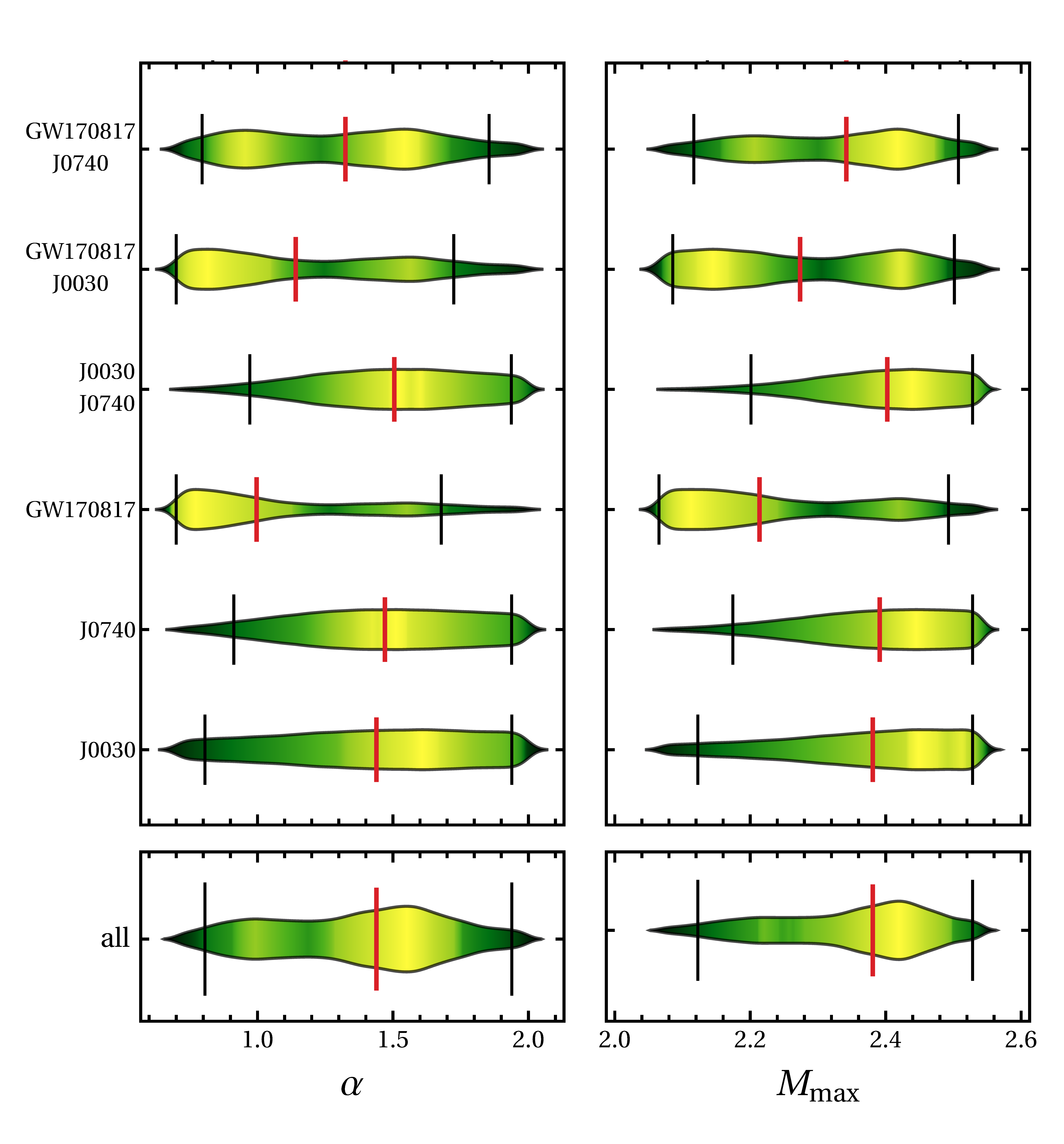
Figure 3: (Left Row) Posterior probability densities for the three-body strength $\alpha$ inferred from different astrophysical datasets. (Right row) Posterior densities for the maximum mass allowed by the EOS corresponding to the inferred distribution of $\alpha$. Bottom panels provide results with all datasets stacked together. Vertical red and black lines identify the median and the the 90% posterior density intervals of each distribution, respectively.

Constraints on $\alpha$, i.e on the microscopic Hamiltonian (1), can be translated into bounds on the stellar macroscopic observables. The right column of Fig. (3) shows, for example, the maximum mass density distributions predicted by the values of $\alpha$ inferred for each dataset. All the observations lead to median values of $M_{\textnormal{max}}\gtrsim 2.2M_{\odot}$, with the multi-messenger analysis yielding a probability distribution with large support for $M_{\textnormal{max}}\sim 2.5M_{\odot}$.

In Fig. 4 we also show the $M$-$R$ density distribution corresponding to the 90% CL of $\alpha$ for the multi-messenger case. Light (dark) colors identify stellar profiles with high (low) probability. Pulsar observations drive the profiles far from the $\alpha=1$ baseline, i.e. towards stiffer NS configurations, with an expected radius $R\gtrsim 12$ km for a prototype NS with $M=1.4M_{\odot}$.

So far our analysis shows that, although the constraining power of current measurements is still limited, astrophysical data are already sensitive to nucleon dynamics. We will therefore explore the insights that can be inferred on three-body nuclear forces exploiting future GW observations of binary inspirals.

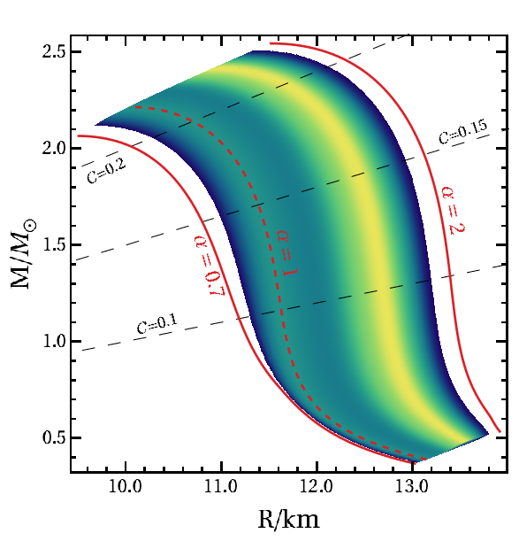
Figure 4: Mass-radius profile density corresponding to the 90% confidence interval of $\alpha$ inferred for the GW-EM multi-messenger analysis. Dark (light) regions correspond to stellar profiles with small (large) probability. As for Fig. 1 red curves identify configurations with specific values of the three-body strength, while dashed black lines correspond to configurations with constant compactness.

As discussed in Sec. III.2 we have simulated two catalogues of $30$ binary NS mergers, observed either by 2G network or by ET, assuming two different values of the three-nucleon strength. Source parameters, i.e. masses and tidal deformabilities, are first recovered with Bilby, and then analyzed by our Bayesian pipeline which samples the posterior distribution of $\alpha$.

Figure 5 shows the posterior densities ${\cal P}(\alpha)$ of each event, for injected NSs with $\alpha=1$, detected by the HLV network. The ability of 2G detectors to discriminate the actual value of the three-body strength substantially depends on both the SNR and on the component masses of the binary. We find that observations with SNR smaller than $\sim 25$ lead $\alpha$ to be almost unconstrained, with the true value always lying outside the 90% confidence interval of the distribution. However, even for strong signals, accurate measurements only occur for low-mass systems with a chirp mass ${\cal M}\lesssim 1.4M_{\odot}$. This is particular evident for the event with the largest SNR ($\sim 35$) in our set. Such binary features two heavy NSs with a chirp mass ${\cal M}\simeq 1.6M_{\odot}$, and provides loose bounds on $\alpha$. Moreover, Fig. 5 shows that, with the exception of four events with SNR$>30$ and ${\cal M}<1.4M_{\odot}$, the remaining posteriors always prefer large values of the three-nucleon strength, at the edge of the upper prior boundary. This particular behavior reflects a systematic bias we find in the posteriors of $\tilde{\Lambda}$ inferred by GW observations for binaries with heavy components, which tend to favour large values of the tidal parameter. Its effect on the marginal distribution of $\alpha$ becomes even more pronounced in the high mass scenario where the tidal deformability becomes less sensitive to variations of $\alpha$. We believe such bias may be induced by our choice of priors on the tidal parameters, which has strong support against the BBH hypothesis $\tilde{\Lambda}=0$, and reflects the physical assumption that compact objects with $m_{1,2}\lesssim 3M_{\odot}$ are neutron stars. Moreover, the stack of multiple GW signals only partially alleviate the bias in favour of large three-body strength. We have indeed combined different observations with SNR larger than 20, finding a mild improvement of the posterior support towards the true value of $\alpha$. The results discussed so far hold qualitatively also when we consider binary NSs simulated with $\alpha=1.3$.

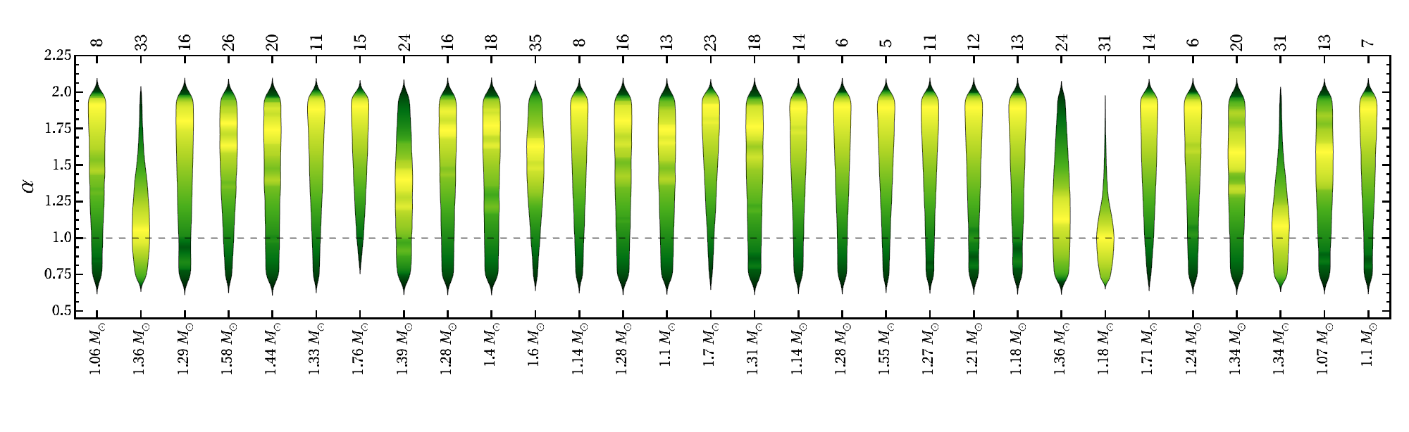
Figure 5: Posterior densities ${\cal P}(\alpha)$ inferred from simulated GW data, assuming $\alpha=1$ (dashed horizontal line). Yellow (green) colors identify region with high (low) probability. Signals are observed by a network HLV of three advanced detectors, with a combined SNR given in the top axis of the plot. Labels in the bottom axis provide the values of the binary chirp masses.

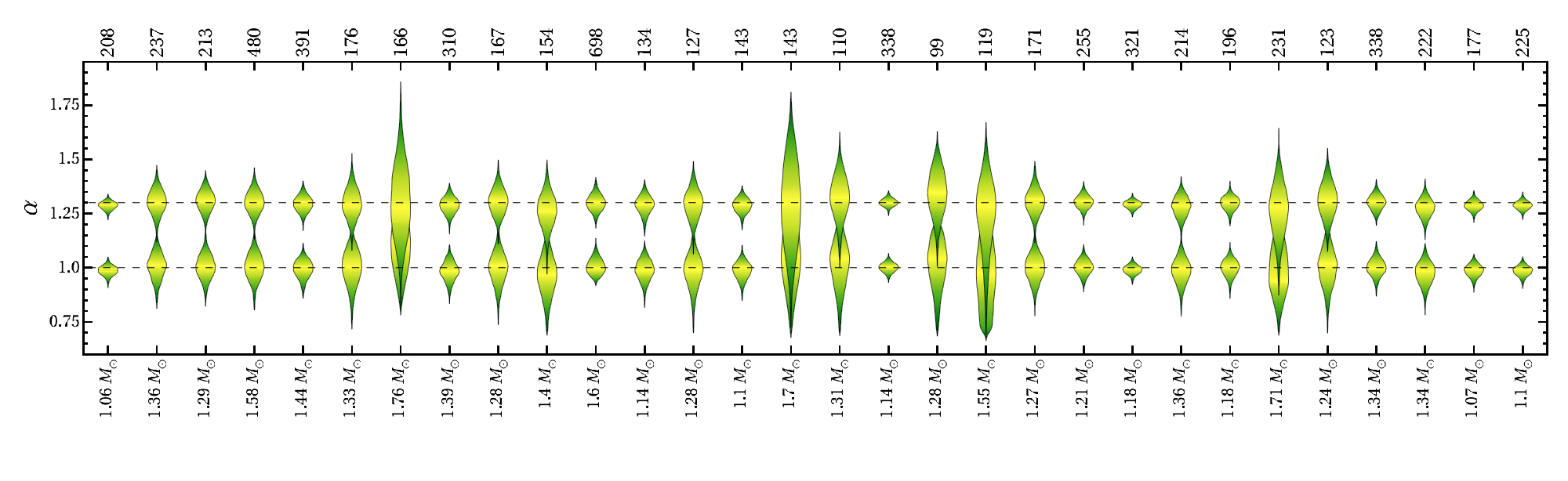
Figure 6: Same as Fig. 5 but assuming that binary NS are observed by the Einstein Telescope. We show results for signals simulated with both $\alpha=1$ and $\alpha=1.3$. Injected values of the three body amplitude are identified by the horizontal dashed lines.

This picture changes dramatically when signals are observed by the Einstein Telescope. Figure 6 shows indeed the distributions of the three-nucleon strength inferred by the 3G detector, for both families of events simulated with $\alpha=1$ and $\alpha=1.3$. The exquisite sensitivity of ET allows to gauge away the bias arising from the 2G network. All the posteriors peak around the injected values of $\alpha$, showing no support on the prior boundaries. In the best (worse) case scenario we find that $\alpha$ can be constrained with $\sim 2\%$ ($\sim 30\%$) of accuracy at $68\%$ confidence level. Such accuracy allows to disentangle the two values of the three-body strength we consider. Even in the most pessimistic cases, where the inferred ${\cal P}(\alpha)$ are not narrow enough to identify a specific value of $\alpha$, stacking of few events would render the distributions clearly distinguishable. Figure 7 shows the posteriors obtained by combining six events of our catalogue leading to loose constraints on $\alpha$. The final posteriors for $\alpha=1$ and $\alpha=1.3$ are clearly separated, with a negligible overlap on the tails.

Such accuracy translates into very narrow constraints on the mass-radius (or equivalently mass-tidal deformability) diagram. As an example, we show in Fig. (8) the $M$-$R$ profile density computed from the values of $\alpha$ inferred from event number 17 of our dataset. A direct comparison with Fig. 4, where a similar plot was made for data from current facilities, provides a clear hint on the possibility to use ET as a new laboratory to study the dynamics of nucleon interactions in the stellar cores.

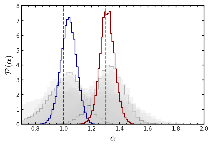
Figure 7: Probability distribution ${\cal P}(\alpha)$ obtained by stacking six events of our dataset as measured by the Einstein Telescope. Empty histograms refer to the full stacked posteriors for signals injected with $\alpha=1$ and $\alpha=1.3$. Empty shaded histograms on the background correspond to the individual posteriors. The vertical dashed lines identify the injected values of $\alpha$.

V Conclusions

We have investigated the sensitivity of NS observations to the strength of repulsive three-nucleon forces, which are known to be critical in determining the stiffness of the nuclear matter EOS at supranuclear densities. Our analysis is based on the AV18 + $\delta v$ + UIX^∗ nuclear Hamiltonian and involves a single free parameter, to be constrained by data, determining the coupling constant appearing in the repulsive contribution to the UIX^∗ potential.

We have performed hierarchical bayesian inference employing the current available multimessenger datasets in order to constrain this parameter. We have then repeated the analysis with a set of simulated GW observations that could be performed by both current (LIGO/Virgo) and future (Einstein Telescope) interferometers at design sensitivity. This analysis has the main purpose to explore the potential of near and next generation facilities into inferring crucial information about the microscopic dynamics of nuclear matter.

The analysis with real data has been carried out employing some of the dataset used in a previous work  [53]. Our results suggest that even if current facilities show a clear sensitivity to small variation of the NNN repulsive potential, they are not accurate enough to capture significant insights. This picture is cross-validated by the population analysis performed with mocked LIGO/Virgo data, with binaries generated with two different values of the three-body strength, $\alpha=1$ and $\alpha=1.3$. Only few, low-mass and high SNR events provide a meaningful constraint on $\alpha$, with posterior distributions correctly peaked around the injected values. Moreover, even for the most constraining event, the inferred posteriors do not allow a clear disentanglement between the two values of $\alpha$ we considered. The picture improves only slightly with the stacking of multiple observations.

These results exhibit a striking upgrade when we assume that the population of binaries is observed by the Einstein Telescope. In most of the cases, the large SNRs obtained by such events in combination with the 3G detector allow the posteriors for the injected values of $\alpha$ to be clearly separated, and only a single observation is needed to resolve them.

Moreover, in the few cases where posteriors overlap, stacking of $\sim 2-3$ observations would allow to unambiguously distinguish between $\alpha=1$ and $\alpha=1.3$. The same conclusion would apply assuming that binaries are detected by the proposed Cosmic Explorer [86, 87]. The large SNRs expected in the 3G era also require a careful assessment of waveform systematics which could bias the parameter reconstruction [88, 89, 90, 85]. However, our results strongly support the evidence that with the upcoming third generation detectors, our understanding of neutron star matter will make a great step forward into the direction of using NS observations to probe fundamental physics at the fermi scale.

Further applications of our approach can be pursued following multiple directions, and in particular considering how constraints on nucleon dynamics would improve by joint analyses of the inspiral and of the post-merger phase, exploiting for the latter either GW oscillation modes [91, 92, 93], or electromagnetic counterparts emitted by the binary remnant [94].

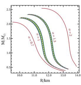
Figure 8: Same as Fig. 4 but for simulated events observed by the Einstein Telescope. The values of $\alpha$ used to build the mass-radius profiles correspond correspond to event number 17 of our catalogue. We show results for both $\alpha=1$ and $\alpha=1.3$. Solid and dashed red curves identify the profiles corresponding to prior boundaries and to the injected values of $\alpha$, respectively.$\alpha$

Appendix A Parametrisation of energy density

In this Appendix, we report the explicit expression of the energy density of nuclear matter employed to carry out our analysis. This expression was originally derived from a fit to the EOSs of SNM and PNM obtained by Akmal et al. [54] using the AV18 + $\delta v$ + UIX^∗ nuclear Hamiltonian and the variational FHNC/SOC formalism.

The energy density of nuclear matter at baryon density $\varrho$ and proton fraction $x_{p}$ is written according to Eqs. (4) and (5)

$$\epsilon(\varrho,x_{p}) =\Big{[}\frac{\hbar^{2}}{2m}+f(\varrho,x_{p})\Big{]}\tau_{p}$$

$$+\Big{[}\frac{\hbar^{2}}{2m}+f(\varrho,1-x_{p})\Big{]}\tau_{n}$$ (17)

$$+g(\varrho,1/2)\Big{[}1-(1-2x_{p})^{2}\Big{]}$$

$$+g(\rho,0)(1-2x_{p})^{2},$$

with

$$\tau_{p} =\varrho x_{p}\ \frac{3}{5}(3\pi^{2}\varrho x_{p})^{2/3}\ ,$$ (18)

$$\tau_{n} =\varrho(1-x_{p})\ \frac{3}{5}[(3\pi^{2}\varrho(1-x_{p})]^{2/3}\ .$$ (19)

The explicit form of the functions $f(\varrho,x_{p})$ and $g(\varrho,x_{p})$ appearing in Eq. (17) are

$$f(\varrho,x_{p})=\left(a_{1}+x_{p}a_{2}\right)\varrho e^{-a_{3}\varrho}$$ (20)

and

$$g(\varrho,x_{p})=\left\{\begin{tabular}[]{ll}$g_{L}(\varrho,x_{p})$&$\varrho\leq\bar{\varrho}$\\ $g_{H}(\varrho,x_{p})$&$\varrho\geq\bar{\varrho}$\end{tabular}\right.\ ,$$ (23)

where

$$g_{L}(\varrho,1/2) =-\varrho^{2}\Big{[}a_{4}+a_{5}\varrho+a_{6}\varrho^{2}+(a_{7}+a_{8}\varrho)e^{-a_{9}^{2}\varrho^{2}}\Big{]}\ ,$$

$$g_{L}(\rho,0) =-\varrho^{2}\Big{(}a_{10}\varrho^{-1}+a_{11}+a_{12}\varrho\Big{)}\ ,$$ (24)

$$g_{H}(\varrho,1/2) =g_{L}(\varrho,1/2)-\varrho^{2}a_{13}(\varrho-a_{14})e^{a_{15}(\rho-a_{14})},$$

$$g_{H}(\rho,0) =g_{L}(\rho,0)-\varrho^{2}a_{16}(\varrho-a_{17}){\rm e}^{a_{18}(\varrho-a_{17})}\ .$$

The density $\bar{\varrho}\lesssim 2\varrho_{0}$ corresponds to the onset of the high-density phase—featuring spin-isospin density waves associated with neutral pion condensation—predicted by the study of Ref. [54].

The values of the parameters appearing in the above equations are given in Table 2

Table 2: Values of the parameters appearing in the definition of the energy density of nuclear matter of Eqs. (17)- (24), expressed in ${\rm MeV\ fm}^{-3}$.

$a_{1}$	$a_{2}$	$a_{3}$	$a_{4}$	$a_{5}$	$a_{6}$
$[{\rm MeV}\ {\rm fm}^{5}]$	$[{\rm MeV}\ {\rm fm}^{5}]$	$[{\rm fm}^{3}]$	$[{\rm MeV}\ {\rm fm}^{3}]$	$[{\rm MeV}\ {\rm fm}^{6}]$	$[{\rm MeV}\ {\rm fm}^{9}]$
89.8	-59.0	0.457	337.2	-382.	-19.1
$a_{7}$	$a_{8}$	$a_{9}$	$a_{10}$	$a_{11}$	$a_{12}$
$[{\rm MeV}\ {\rm fm}^{3}]$	$[{\rm MeV}\ {\rm fm}^{6}]$	$[{\rm fm}^{3}]$	$[{\rm MeV}]$	$[{\rm MeV}\ {\rm fm}^{3}]$	$[{\rm MeV}\ {\rm fm}^{6}]$
69.0	-33.0	6.4	0.35	214.6	-384.0
$a_{13}$	$a_{14}$	$a_{15}$	$a_{16}$	$a_{17}$	$a_{18}$
$[{\rm MeV}\ {\rm fm}^{6}]$	$[{\rm fm}^{-3}]$	$[{\rm MeV}\ {\rm fm}^{6}]$	$[{\rm MeV}\ {\rm fm}^{6}]$	$[{\rm MeV}]$	$[{\rm fm}^{3}]$
175.0	0.32	-1.45	287.0	0.195	-1.54

References

- [1] H. T. Cromartie et al., “Relativistic Shapiro delay measurements of an extremely massive millisecond pulsar,” arXiv:1904.06759.
- [2] E. Fonseca et al., “Refined Mass and Geometric Measurements of the High-mass PSR J0740+6620,” Astrophys. J. Lett. 915 no. 1, (2021) L12, arXiv:2104.00880 [astro-ph.HE].
- [3] T. E. Riley et al., “A View of PSR J0030+0451: Millisecond Pulsar Parameter Estimation,” Astrophys. J. Lett. 887 no. 1, (2019) L21, arXiv:1912.05702 [astro-ph.HE].
- [4] M. C. Miller et al., “PSR J0030+0451 Mass and Radius from Data and Implications for the Properties of Neutron Star Matter,” Astrophys. J. Lett. 887 no. 1, (2019) L24, arXiv:1912.05705 [astro-ph.HE].
- [5] T. E. Riley et al., “A NICER View of the Massive Pulsar PSR J0740+6620 Informed by Radio Timing and XMM-Newton Spectroscopy,” Astrophys. J. Lett. 918 no. 2, (2021) L27, arXiv:2105.06980 [astro-ph.HE].
- [6] M. C. Miller et al., “The Radius of PSR J0740+6620 from NICER and XMM-Newton Data,” Astrophys. J. Lett. 918 no. 2, (2021) L28, arXiv:2105.06979 [astro-ph.HE].
- [7] LIGO Scientific, Virgo Collaboration, B. P. Abbott et al., “Properties of the binary neutron star merger GW170817,” Phys. Rev. X 9 no. 1, (2019) 011001, arXiv:1805.11579 [gr-qc].
- [8] LIGO Scientific, Virgo Collaboration, B. P. Abbott et al., “GW170817: Observation of Gravitational Waves from a Binary Neutron Star Inspiral,” Phys. Rev. Lett. 119 no. 16, (2017) 161101, arXiv:1710.05832 [gr-qc].
- [9] LIGO Scientific, Virgo Collaboration, B. P. Abbott et al., “GW190425: Observation of a Compact Binary Coalescence with Total Mass ,” Astrophys. J. Lett. 892 no. 1, (2020) L3, arXiv:2001.01761 [astro-ph.HE].
- [10] T. Hinderer, “Tidal Love numbers of neutron stars,” Astrophys. J. 677 (2008) 1216–1220, arXiv:0711.2420 [astro-ph].
- [11] T. Damour and A. Nagar, “Relativistic tidal properties of neutron stars,” Phys. Rev. D 80 (2009) 084035, arXiv:0906.0096 [gr-qc].
- [12] T. Binnington and E. Poisson, “Relativistic theory of tidal Love numbers,” Phys. Rev. D 80 (2009) 084018, arXiv:0906.1366 [gr-qc].
- [13] E. E. Flanagan and T. Hinderer, “Constraining neutron star tidal Love numbers with gravitational wave detectors,” Phys. Rev. D 77 (2008) 021502, arXiv:0709.1915 [astro-ph].
- [14] J. E. Vines and E. E. Flanagan, “Post-1-Newtonian quadrupole tidal interactions in binary systems,” Phys. Rev. D 88 (2013) 024046, arXiv:1009.4919 [gr-qc].
- [15] J. Vines, E. E. Flanagan, and T. Hinderer, “Post-1-Newtonian tidal effects in the gravitational waveform from binary inspirals,” Phys. Rev. D 83 (2011) 084051, arXiv:1101.1673 [gr-qc].
- [16] G. Colò, “The compression modes in atomic nuclei and their relevance for the nuclear equation of state,” Physics of Particles and Nuclei 39 no. 2, (Mar., 2008) 286–305.
- [17] B.-A. Li and X. Han, “Constraining the neutron-proton effective mass splitting using empirical constraints on the density dependence of nuclear symmetry energy around normal density,” Phys. Lett. B 727 (2013) 276–281, arXiv:1304.3368 [nucl-th].
- [18] P. Russotto et al., “Results of the ASY-EOS experiment at GSI: The symmetry energy at suprasaturation density,” Phys. Rev. C 94 no. 3, (2016) 034608, arXiv:1608.04332 [nucl-ex].
- [19] M. B. Tsang, Y. Zhang, P. Danielewicz, M. Famiano, Z. Li, W. G. Lynch, and A. W. Steiner, “Constraints on the density dependence of the symmetry energy,” Phys. Rev. Lett. 102 (2009) 122701, arXiv:0811.3107 [nucl-ex].
- [20] P. Danielewicz, R. Lacey, and W. G. Lynch, “Determination of the equation of state of dense matter,” Science 298 (2002) 1592–1596, arXiv:nucl-th/0208016.
- [21] B. A. Brown, “Constraints on the Skyrme Equations of State from Properties of Doubly Magic Nuclei,” Phys. Rev. Lett. 111 no. 23, (2013) 232502, arXiv:1308.3664 [nucl-th].
- [22] Z. Zhang and L.-W. Chen, “Constraining the symmetry energy at subsaturation densities using isotope binding energy difference and neutron skin thickness,” Phys. Lett. B 726 (2013) 234–238, arXiv:1302.5327 [nucl-th].
- [23] PREX Collaboration, D. Adhikari et al., “Accurate Determination of the Neutron Skin Thickness of 208Pb through Parity-Violation in Electron Scattering,” Phys. Rev. Lett. 126 no. 17, (2021) 172502, arXiv:2102.10767 [nucl-ex].
- [24] E. Annala, T. Gorda, A. Kurkela, and A. Vuorinen, “Gravitational-wave constraints on the neutron-star-matter Equation of State,” Phys. Rev. Lett. 120 no. 17, (2018) 172703, arXiv:1711.02644 [astro-ph.HE].
- [25] B. Margalit and B. D. Metzger, “Constraining the Maximum Mass of Neutron Stars From Multi-Messenger Observations of GW170817,” Astrophys. J. Lett. 850 no. 2, (2017) L19, arXiv:1710.05938 [astro-ph.HE].
- [26] D. Radice, A. Perego, F. Zappa, and S. Bernuzzi, “GW170817: Joint Constraint on the Neutron Star Equation of State from Multimessenger Observations,” Astrophys. J. Lett. 852 no. 2, (2018) L29, arXiv:1711.03647 [astro-ph.HE].
- [27] A. Bauswein, O. Just, H.-T. Janka, and N. Stergioulas, “Neutron-star radius constraints from GW170817 and future detections,” Astrophys. J. Lett. 850 no. 2, (2017) L34, arXiv:1710.06843 [astro-ph.HE].
- [28] Y. Lim and J. W. Holt, “Neutron star tidal deformabilities constrained by nuclear theory and experiment,” Phys. Rev. Lett. 121 no. 6, (2018) 062701, arXiv:1803.02803 [nucl-th].
- [29] Y. Lim, A. Bhattacharya, J. W. Holt, and D. Pati, “Radius and equation of state constraints from massive neutron stars and GW190814,” Phys. Rev. C 104 no. 3, (2021) L032802, arXiv:2007.06526 [nucl-th].
- [30] E. R. Most, L. R. Weih, L. Rezzolla, and J. Schaffner-Bielich, “New constraints on radii and tidal deformabilities of neutron stars from GW170817,” Phys. Rev. Lett. 120 no. 26, (2018) 261103, arXiv:1803.00549 [gr-qc].
- [31] S. De, D. Finstad, J. M. Lattimer, D. A. Brown, E. Berger, and C. M. Biwer, “Tidal Deformabilities and Radii of Neutron Stars from the Observation of GW170817,” Phys. Rev. Lett. 121 no. 9, (2018) 091102, arXiv:1804.08583 [astro-ph.HE]. [Erratum: Phys.Rev.Lett. 121, 259902 (2018)].
- [32] E. Annala, T. Gorda, A. Kurkela, J. Nättilä, and A. Vuorinen, “Evidence for quark-matter cores in massive neutron stars,” Nature Phys. 16 no. 9, (2020) 907–910, arXiv:1903.09121 [astro-ph.HE].
- [33] G. Raaijmakers et al., “Constraining the dense matter equation of state with joint analysis of NICER and LIGO/Virgo measurements,” Astrophys. J. Lett. 893 no. 1, (2020) L21, arXiv:1912.11031 [astro-ph.HE].
- [34] M. C. Miller, C. Chirenti, and F. K. Lamb, “Constraining the equation of state of high-density cold matter using nuclear and astronomical measurements,” arXiv:1904.08907 [astro-ph.HE].
- [35] B. Kumar and P. Landry, “Inferring neutron star properties from GW170817 with universal relations,” Phys. Rev. D 99 no. 12, (2019) 123026, arXiv:1902.04557 [gr-qc].
- [36] M. Fasano, T. Abdelsalhin, A. Maselli, and V. Ferrari, “Constraining the Neutron Star Equation of State Using Multiband Independent Measurements of Radii and Tidal Deformabilities,” Phys. Rev. Lett. 123 no. 14, (2019) 141101, arXiv:1902.05078 [astro-ph.HE].
- [37] P. Landry, R. Essick, and K. Chatziioannou, “Nonparametric constraints on neutron star matter with existing and upcoming gravitational wave and pulsar observations,” Phys. Rev. D 101 no. 12, (2020) 123007, arXiv:2003.04880 [astro-ph.HE].
- [38] H. Güven, K. Bozkurt, E. Khan, and J. Margueron, “Multimessenger and multiphysics Bayesian inference for the GW170817 binary neutron star merger,” Phys. Rev. C 102 no. 1, (2020) 015805, arXiv:2001.10259 [nucl-th].
- [39] S. Traversi, P. Char, and G. Pagliara, “Bayesian Inference of Dense Matter Equation of State within Relativistic Mean Field Models using Astrophysical Measurements,” Astrophys. J. 897 (2020) 165, arXiv:2002.08951 [astro-ph.HE].
- [40] G. Raaijmakers, S. K. Greif, K. Hebeler, T. Hinderer, S. Nissanke, A. Schwenk, T. E. Riley, A. L. Watts, J. M. Lattimer, and W. C. G. Ho, “Constraints on the Dense Matter Equation of State and Neutron Star Properties from NICER’s Mass–Radius Estimate of PSR J0740+6620 and Multimessenger Observations,” Astrophys. J. Lett. 918 no. 2, (2021) L29, arXiv:2105.06981 [astro-ph.HE].
- [41] J. Zimmerman, Z. Carson, K. Schumacher, A. W. Steiner, and K. Yagi, “Measuring Nuclear Matter Parameters with NICER and LIGO/Virgo,” arXiv:2002.03210 [astro-ph.HE].
- [42] H. O. Silva, A. M. Holgado, A. Cárdenas-Avendaño, and N. Yunes, “Astrophysical and theoretical physics implications from multimessenger neutron star observations,” Phys. Rev. Lett. 126 no. 18, (2021) 181101, arXiv:2004.01253 [gr-qc].
- [43] A. Sabatucci and O. Benhar, “Tidal Deformation of Neutron Stars from Microscopic Models of Nuclear Dynamics,” Phys. Rev. C 101 no. 4, (2020) 045807, arXiv:2001.06294 [nucl-th].
- [44] D. Blaschke, A. Ayriyan, D. E. Alvarez-Castillo, and H. Grigorian, “Was GW170817 a Canonical Neutron Star Merger? Bayesian Analysis with a Third Family of Compact Stars,” Universe 6 no. 6, (2020) 81, arXiv:2005.02759 [astro-ph.HE].
- [45] S.-P. Tang, J.-L. Jiang, W.-H. Gao, Y.-Z. Fan, and D.-M. Wei, “Constraint on phase transition with the multimessenger data of neutron stars,” Phys. Rev. D 103 no. 6, (2021) 063026, arXiv:2009.05719 [astro-ph.HE].
- [46] B. Biswas, P. Char, R. Nandi, and S. Bose, “Towards mitigation of apparent tension between nuclear physics and astrophysical observations by improved modeling of neutron star matter,” Phys. Rev. D 103 no. 10, (2021) 103015, arXiv:2008.01582 [astro-ph.HE].
- [47] C. Pacilio, A. Maselli, M. Fasano, and P. Pani, “Ranking Love Numbers for the Neutron Star Equation of State: The Need for Third-Generation Detectors,” Phys. Rev. Lett. 128 no. 10, (2022) 101101, arXiv:2104.10035 [gr-qc].
- [48] T. Malik and C. Providência, “Bayesian inference of signatures of hyperons inside neutron stars,” arXiv:2205.15843 [nucl-th].
- [49] S. Altiparmak, C. Ecker, and L. Rezzolla, “On the Sound Speed in Neutron Stars,” arXiv:2203.14974 [astro-ph.HE].
- [50] P. K. Gupta, A. Puecher, P. T. H. Pang, J. Janquart, G. Koekoek, and C. Broeck Van Den, “Determining the equation of state of neutron stars with Einstein Telescope using tidal effects and r-mode excitations from a population of binary inspirals,” arXiv:2205.01182 [gr-qc].
- [51] L. Baiotti, “Gravitational waves from neutron star mergers and their relation to the nuclear equation of state,” Prog. Part. Nucl. Phys. 109 (2019) 103714, arXiv:1907.08534 [astro-ph.HE].
- [52] K. Chatziioannou, “Neutron star tidal deformability and equation of state constraints,” Gen. Rel. Grav. 52 no. 11, (2020) 109, arXiv:2006.03168 [gr-qc].
- [53] A. Maselli, A. Sabatucci, and O. Benhar, “Constraining three-nucleon forces with multimessenger data,” Phys. Rev. C 103 no. 6, (2021) 065804, arXiv:2010.03581 [astro-ph.HE].
- [54] A. Akmal, V.R. Pandharipande, and D.G. Ravenhall, “Equation of state of nucleon matter and neutron star structure,” Phys. Rev. C 58 (1998) 1804.
- [55] B. S. Pudliner, V. R. Pandharipande, J. Carlson, and R. B. Wiringa, “Quantum Monte Carlo calculations of A ¡= 6 nuclei,” Phys. Rev. Lett. 74 (1995) 4396–4399.
- [56] J. Carlson, V. R. Pandharipande, and R. B. Wiringa Nucl. Phys. A 401 (1983) 59.
- [57] M. Punturo et al., “The Einstein Telescope: A third-generation gravitational wave observatory,” Class. Quant. Grav. 27 (2010) 194002.
- [58] S. Hild et al., “Sensitivity Studies for Third-Generation Gravitational Wave Observatories,” Class. Quant. Grav. 28 (2011) 094013, arXiv:1012.0908 [gr-qc].
- [59] M. Maggiore et al., “Science Case for the Einstein Telescope,” JCAP 03 (2020) 050, arXiv:1912.02622 [astro-ph.CO].
- [60] J. Carlson, S. Gandolfi, F. Pederiva, S. C. Pieper, R. Schiavilla, K. E. Schmidt, and R. B. Wiringa Rev. Mod. Phys. 87 (2015) 1067.
- [61] O. Benhar Int. J. Mod. Phys. E 9 (2021) 2130009.
- [62] R. Essick, I. Tews, P. Landry, S. Reddy, and D. E. Holz, “Direct astrophysical tests of chiral effective field theory at supranuclear densities,” Phys. Rev. C 102 (Nov, 2020) 055803. https://link.aps.org/doi/10.1103/PhysRevC.102.055803.
- [63] R. B. Wiringa, V. G. J. Stoks, and R. Schiavilla, “An Accurate nucleon-nucleon potential with charge independence breaking,” Phys. Rev. C 51 (1995) 38–51.
- [64] A. Akmal and V. R. Pandharipande, “Spin-isospin structure and pion condensation in nucleon matter,” Phys. Rev. C 56 (Oct, 1997) 2261–2279. https://link.aps.org/doi/10.1103/PhysRevC.56.2261.
- [65] Tolman, R. C., “Static solutions of Einstein’s field equations for spheres of fluid,” Phys. Rev. 55 (1939) 364.
- [66] Oppenheimer, J. R. and Volkoff, G. M., “On massive neutron cores,” Phys. Rev. 55 (1939) 374.
- [67] A. Sabatucci and O. Benhar, “Tidal deformation of neutron stars from microscopic models of nuclear dynamics,” Phys. Rev. C 101 (Apr, 2020) 045807. https://link.aps.org/doi/10.1103/PhysRevC.101.045807.
- [68] J. Fujita and H. Miyazawa, “Pion Theory of Three-Body Forces,” Prog. Theor. Phys. 17 (1957) 360–365.
- [69] J. Forest, V. R. Pandharipande, and J. L. Friar Phys. Rev. C 52 (1995) 568.
- [70] V. R. Pandharipande and R. B. Wiringa Rev. Mod. Phys. 51 (1979) 821.
- [71] O. Benhar and A. Lovato, “Perturbation theory of nuclear matter with a microscopic effective interaction,” Phys. Rev. C 96 (2017) 054301.
- [72] J. Carlson, S. Gandolfi, F. Pederiva, S. C. Pieper, R. Schiavilla, K. E. Schmidt, and R. B. Wiringa, “Quantum monte carlo methods for nuclear physics,” Rev. Mod. Phys. 87 (Sep, 2015) 1067–1118. https://link.aps.org/doi/10.1103/RevModPhys.87.1067.
- [73] D. Foreman-Mackey, D. W. Hogg, D. Lang, and J. Goodman, “emcee: The MCMC Hammer,” PASP 125 no. 925, (Mar., 2013) 306, arXiv:1202.3665 [astro-ph.IM].
- [74] T. E. Riley, A. L. Watts, S. Bogdanov, P. S. Ray, R. M. Ludlam, S. Guillot, Z. Arzoumanian, C. L. Baker, A. V. Bilous, D. Chakrabarty, K. C. Gendreau, A. K. Harding, W. C. G. Ho, J. M. Lattimer, S. M. Morsink, and T. E. Strohmayer, “A NICER View of PSR J0030+0451: Nested Samples for Millisecond Pulsar Parameter Estimation,” Mar., 2020. https://doi.org/10.5281/zenodo.5506838.
- [75] T. E. Riley, A. L. Watts, P. S. Ray, S. Bogdanov, S. Guillot, S. M. Morsink, A. V. Bilous, Z. Arzoumanian, D. Choudhury, J. S. Deneva, K. C. Gendreau, A. K. Harding, W. C. Ho, J. M. Lattimer, M. Loewenstein, R. M. Ludlam, C. B. Markwardt, T. Okajima, C. Prescod-Weinstein, R. A. Remillard, M. T. Wolff, E. Fonseca, H. T. Cromartie, M. Kerr, T. T. Pennucci, A. Parthasarathy, S. Ransom, I. Stairs, L. Guillemot, and I. Cognard, “A NICER View of the Massive Pulsar PSR J0740+6620 Informed by Radio Timing and XMM-Newton Spectroscopy: Nested Samples for Millisecond Pulsar Parameter Estimation,” Apr., 2021. https://doi.org/10.5281/zenodo.4697625.
- [76] M. Miller, F. K. Lamb, A. J. Dittmann, S. Bogdanov, Z. Arzoumanian, K. C. Gendreau, S. Guillot, W. C. G. Ho, J. M. Lattimer, S. M. Morsink, P. S. Ray, M. T. Wolff, C. L. Baker, T. Cazeau, S. Manthripragada, C. B. Markwardt, T. Okajima, S. Pollard, I. Cognard, H. T. Cromartie, E. Fonseca, L. Guillemot, M. Kerr, A. Parthasarathy, T. T. Pennucci, S. Ransom, I. Stairs, and M. Loewenstein, “NICER PSR J0740+6620 Illinois-Maryland MCMC Samples,” Apr., 2021. https://doi.org/10.5281/zenodo.4670689.
- [77] G. Raaijmakers, S. Greif, K. Hebeler, T. Hinderer, S. Nissanke, A. Schwenk, T. Riley, J. Lattimer, and W. Ho, “Constraints on the dense matter equation of state and neutron star properties from NICER’s mass- radius estimate of PSR J0740+6620 and multimessenger observations: posterior samples and scripts for generating plots,” Apr., 2021. https://doi.org/10.5281/zenodo.4696232.
- [78] D. Wysocki, R. O’Shaughnessy, L. Wade, and J. Lange, “Inferring the neutron star equation of state simultaneously with the population of merging neutron stars,” arXiv:2001.01747 [gr-qc].
- [79] M. Pitkin, S. Reid, S. Rowan, and J. Hough, “Gravitational Wave Detection by Interferometry (Ground and Space),” Living Rev. Rel. 14 (2011) 5, arXiv:1102.3355 [astro-ph.IM].
- [80] L. Wade, J. D. E. Creighton, E. Ochsner, B. D. Lackey, B. F. Farr, T. B. Littenberg, and V. Raymond, “Systematic and statistical errors in a bayesian approach to the estimation of the neutron-star equation of state using advanced gravitational wave detectors,” Phys. Rev. D89 no. 10, (2014) 103012, arXiv:1402.5156 [gr-qc].
- [81] G. Ashton et al., “BILBY: A user-friendly Bayesian inference library for gravitational-wave astronomy,” Astrophys. J. Suppl. 241 no. 2, (2019) 27, arXiv:1811.02042 [astro-ph.IM].
- [82] I. M. Romero-Shaw et al., “Bayesian inference for compact binary coalescences with bilby: validation and application to the first LIGO–Virgo gravitational-wave transient catalogue,” Mon. Not. Roy. Astron. Soc. 499 no. 3, (2020) 3295–3319, arXiv:2006.00714 [astro-ph.IM].
- [83] T. Dietrich, S. Bernuzzi, and W. Tichy, “Closed-form tidal approximants for binary neutron star gravitational waveforms constructed from high-resolution numerical relativity simulations,” Phys. Rev. D 96 no. 12, (2017) 121501, arXiv:1706.02969 [gr-qc].
- [84] T. Dietrich et al., “Matter imprints in waveform models for neutron star binaries: Tidal and self-spin effects,” Phys. Rev. D 99 no. 2, (2019) 024029, arXiv:1804.02235 [gr-qc].
- [85] G. Castro, L. Gualtieri, A. Maselli, and P. Pani, “Impact and detectability of spin-tidal couplings in neutron star inspirals,” arXiv:2204.12510 [gr-qc].
- [86] R. Essick, S. Vitale, and M. Evans, “Frequency-dependent responses in third generation gravitational-wave detectors,” Phys. Rev. D 96 no. 8, (2017) 084004, arXiv:1708.06843 [gr-qc].
- [87] LIGO Scientific Collaboration, B. P. Abbott et al., “Exploring the Sensitivity of Next Generation Gravitational Wave Detectors,” Class. Quant. Grav. 34 no. 4, (2017) 044001, arXiv:1607.08697 [astro-ph.IM].
- [88] K. Chatziioannou, “Uncertainty limits on neutron star radius measurements with gravitational waves,” Phys. Rev. D 105 no. 8, (2022) 084021, arXiv:2108.12368 [gr-qc].
- [89] R. Gamba, M. Breschi, S. Bernuzzi, M. Agathos, and A. Nagar, “Waveform systematics in the gravitational-wave inference of tidal parameters and equation of state from binary neutron star signals,” Phys. Rev. D 103 no. 12, (2021) 124015, arXiv:2009.08467 [gr-qc].
- [90] T. Narikawa, N. Uchikata, K. Kawaguchi, K. Kiuchi, K. Kyutoku, M. Shibata, and H. Tagoshi, “Reanalysis of the binary neutron star mergers GW170817 and GW190425 using numerical-relativity calibrated waveform models,” Phys. Rev. Res. 2 no. 4, (2020) 043039, arXiv:1910.08971 [gr-qc].
- [91] S. H. Völkel and C. J. Krüger, “Constraining the Nuclear Equation of State from Rotating Neutron Stars,” arXiv:2203.05555 [gr-qc].
- [92] L. Tonetto, A. Sabatucci, and O. Benhar, “Impact of three-nucleon forces on gravitational wave emission from neutron stars,” Phys. Rev. D 104 no. 8, (2021) 083034, arXiv:2106.16131 [nucl-th].
- [93] M. Wijngaarden, K. Chatziioannou, A. Bauswein, J. A. Clark, and N. J. Cornish, “Probing neutron stars with the full premerger and postmerger gravitational wave signal from binary coalescences,” Phys. Rev. D 105 no. 10, (2022) 104019, arXiv:2202.09382 [gr-qc].
- [94] M. Breschi, A. Perego, S. Bernuzzi, W. Del Pozzo, V. Nedora, D. Radice, and D. Vescovi, “AT2017gfo: Bayesian inference and model selection of multicomponent kilonovae and constraints on the neutron star equation of state,” Mon. Not. Roy. Astron. Soc. 505 no. 2, (2021) 1661–1677, arXiv:2101.01201 [astro-ph.HE].