Resonance production in partial chemical equilibrium

Abstract

In high energy collisions, a dense, strongly interacting medium could be created, the quark gluon plasma. In rapid expansion, from the soup of quarks and gluons a gas of resonance and stable particles is formed at the chemical freeze-out and after that, as the system cools down, the kinetic freeze-out takes place and interaction between particles ceases. By measuring resonance ratios one could get information about the dominant physical processes in the intermediate temperature ranges, i.e. between the chemical and kinetic freeze-out. These quantities are measured at RHIC and LHC energies. In the present analysis we employ the hadron resonance gas model assuming partial chemical equilibrium to characterize these measured data. We calculate the ratios of several resonances to their stable counterpart and compare these model calculations to available experimental data.

I Introduction

Collisions of atomic nuclei at ultrarelativistic energies provide an environment for studying the properties of very hot and dense strongly interacting matter. Hadrons, which escape from the fireball after its breakup carry direct information about its dynamical state at the end of the evolution.

Resonances mediate the interactions among hadrons. Thus a measurement of their production in nuclear collisions carries information about the interactions that are going on in the hot medium, especially towards the end of its evolution.

A standard baseline that is used for the interpretation of hadron data is built upon the idea of statistical production of hadrons. It has been shown, that at lowest order of the virial expansion, interactions between ground state hadrons can be incorporated into the statistical model by introducing the resonances into the partition function and treating them as free particles Dashen et al. (1969).

Statistical model has been quite successful in describing the abundances of ground state hadrons Becattini et al. (2006); Abelev et al. (2009a, 2013); Andronic et al. (2019, 2018); Bhattacharyya et al. (2019, 2020), and even—which is rather puzzling—clusters like deuterons, tritons, or ³He Acharya et al. (2020); Biswas (2020). It leads to the introduction of the so-called chemical freeze-out. This is the thermodynamic state of the fireball, specified by its temperature, chemical potentials, and volume, which reproduces the observed abundances of stable hadrons. It should be stressed that it also accounts for the production of stable hadrons from (chains of) decays of resonances, which are present in the thermalised fireball. The average number of resonances is also set by the same parameters.

However, transverse momentum spectra seem to indicate hadron production from locally thermalised fireball at much lower temperature Melo and Tomášik (2016). The fireball thus cools down in the hadronic phase from the chemical freeze-out down to the thermal freeze-out, while the final state abundances of ground state hadrons must be fixed. Note, though, that there are other studies, also, which do not indicate such a low kinetic freeze-out temperature Mazeliauskas and Vislavicius (2020). The issue is thus somewhat inconclusive at the moment.

In an extended hadron phase, a decrease of the temperature affects the ratio of resonance abundances to those of stable hadrons. The condition of fixed stable species abundance implies specific prescription for non-equilibrium chemical potentials of individual species Bebie et al. (1992). Such a state is usually described as Partial Chemical Equilibrium (PCE). Consequently, it also influences the resonance-to-stable ratios of abundances. Hence, the measurement of this ratio would probe such a scenario. One could argue that the proper treatment of resonance production would be by employing transport simulation. This would also be the relevant treatment for the case that resonances cannot be reliably measured due to rescattering of their decay products Knospe et al. (2016). Nevertheless, we want to explore PCE as a simple and economic alternative to the complicated and computationally expensive transport simulations. In this study we thus investigate the limits of applicability of the PCE model.

In this paper we therefore entertain the idea of a scenario with an extended hadronic phase and PCE. For this scenario we calculate the production of resonances and determine the resonance-to-stable ratios for selected types of resonances which have been measured experimentally. Within the used model, such a ratio can be assigned to a value of the temperature, although this may not always be possible. The extracted temperatures can be compared with those of kinetic freeze-out in order to see if the instantaneous freeze-out is a good approximation or to what extent it is distant from reality.

We describe the basics of the statistical model with PCE in Section II. In Section III, we explain our selection of experimental data and the method of comparison of theoretical results to them. The actual results are summarised in Section IV, followed by conclusions in Section V.

II Description of the model

II.1 Hadron resonance gas model

The analysis is performed in framework of the hadron resonance gas model Dashen et al. (1969). The model is given by the logarithm of its partition function:

$$\ln Z(T,\mu,V) =\sum_{i}\ln Z_{i}(T,\mu_{i},V)$$

$$=\sum_{i}\pm\frac{g_{i}V}{2\pi^{2}}\int_{0}^{\infty}\,p^{2}\ln\left[1\pm e^{\frac{\mu_{i}-\varepsilon(p)}{T}}\right]dp$$ (1)

where the sum runs over the stable and resonance hadron species, $p$ is the momentum, $\varepsilon(p)=\sqrt{p^{2}+m_{i}^{2}}$ is the energy, $g_{i}$ is the spin degeneracy factor, and the $\pm$ sign corresponds to the Bose/Fermi case respectively. The chemical potentials $\mu_{i}$ are set for every particle species. From the partition function, based on thermodynamical identities, one can get the partial pressure, energy density, and number density for species $i$

$$P_{i} =\frac{T\ln(Z_{i})}{V}$$ (2)

$$e_{i} =\frac{g_{i}}{2\pi^{2}}\int_{0}^{\infty}\frac{p^{2}\varepsilon(p)}{\exp\left[\frac{\varepsilon(p)-\mu_{i}}{T}\right]\pm 1}dp$$ (3)

$$n_{i} =\frac{g_{i}}{2\pi^{2}}\int_{0}^{\infty}\frac{p^{2}}{\exp\left[\frac{\varepsilon(p)-\mu_{i}}{T}\right]\pm 1}dp.$$ (4)

In our calculations , we shall also need the entropy density, which can be determined from the thermodynamic relation

$$s=\sum_{i}\frac{P_{i}+e_{i}-n_{i}\mu_{i}}{T}$$ (5)

where the sum, again, runs over the hadron species including the resonances.

II.2 Partial chemical equilibrium

During the time evolution of the fireball, two freeze-out stages take place. As it cools down and reaches certain temperature, the chemical freeze-out happens when inelastic processes cease. Data indicate that this happens in the proximity of the hadronisation transition Andronic et al. (2018). After further cooling, the kinetic freeze-out is reached where all interactions between the particles are assumed to disappear.

Measurements showed that the kinetic and the chemical freeze-out temperature differ by about 50–70 MeV/c² (see in Ref. Melo and Tomášik (2020)). However, the multiplicities are frozen at the chemical freeze-out temperature. Consequently, the subsequent cooling and expansion should evolve in such a way that the average effective number of the stable particle species is conserved. Here, the hadrons which are produced from decays of unstable resonances are also included. This can be formulated as

$$\langle N^{\textmd{eff}}_{h}\rangle=\sum_{i}c_{i\rightarrow h}\langle N_{i}\rangle.$$ (6)

The sums runs over both the stable as well as resonance hadron species and $\langle N_{i}\rangle$ is the average number of species $i$. The weights $c_{i\rightarrow h}$ mean the average number of hadron $h$ that originates from one resonance $i$. (N.B.: $c_{h\rightarrow h}=1$.)

Since the abundance ratios between stable hadrons are kept constant even in spite of decreasing temperature, this is a non-equilibrium feature which will be parametrised with the help of chemical potentials. However, PCE also means that the resonances are in equilibrium with their daughter particles. Consequently, chemical potential of resonance species is given by the sum of chemical potentials of its daughters. A simple example is the $\Delta^{++}$ with only one decay channel into a proton and pion

$$\Delta^{++} \rightarrow p+\pi^{+}$$

$$\mu_{\Delta^{++}} =\mu_{p}+\mu_{\pi^{+}}\,.$$

Resonances with more then one decay channel are also considered. Their chemical potential is then obtained as weighted average with branching ratios as weights. Let us use $\Delta^{+}$ as an example

$$\Delta^{+} \rightarrow n+\pi^{+}\hskip 14.22636pt\textmd{or}\hskip 14.22636pt\Delta^{+}\rightarrow p+\pi^{0}$$

$$\mu_{\Delta^{+}} =a_{[\Delta^{+}\rightarrow n+\pi^{+}]}(\mu_{n}+\mu_{\pi^{+}})$$

$$\qquad+a_{[\Delta^{+}\rightarrow p+\pi^{0}]}(\mu_{p}+\mu_{\pi^{0}})\,.$$

where the numbers $a_{[...]}$ denote the branching ratios. After summing up contributions from chain decays of heavier resonances, the chemical potential of resonance species $i$ is given as

$$\mu_{i}=\sum_{h}c_{i\rightarrow h}\mu_{h}\,,$$ (7)

where the sum runs through all stable hadrons species.

As we mentioned above, the effective numbers of stable hadrons are conserved. This requires that each stable species obtain their own $\mu_{h}$ as the system cools down. However, chemical potentials as functions of temperature cannot be calculated from the condition of constant $\langle N^{\textmd{eff}}_{h}\rangle$, solely, because the numbers also depend on volume, which is unknown and also changes. The trick is in the assumption of isentropic expansion and the use of entropy $S$ as another conserved quantity. The volume-independent ratio $\langle N^{\textmd{eff}}_{h}\rangle/S$ is then also conserved. We can thus work with the corresponding densities

$$\frac{\langle N^{\textmd{eff}}_{h}\rangle}{S} =\frac{n^{\textmd{eff}}_{h}}{s}$$ (8)

$$n^{\textmd{eff}}_{h} =\sum_{i}c_{i\rightarrow h}n_{i}\,,$$ (9)

where $s$ can be determined from eq. (5) and $n_{i}$’s from eq. (4). Hence, the following system of algebraic equations can be used for the calculation of $\mu_{h}(T)$’s

$$\frac{n^{\textmd{eff}}_{h}(T)}{s(T)}=\left.\frac{n^{\textmd{eff}}_{h}(T)}{s(T)}\right|_{T=T_{\textmd{chem}}}$$ (10)

where $T_{\textmd{chem}}$ is the temperature of the chemical freeze-out and the equations are indexed by $h$.

The starting point of the evolution is given at the chemical freeze-out. Chemical equilibrium with the temperature ($T_{\textmd{chem}}$), baryochemical potential ($\mu_{B}$), the strangeness chemical potential ($\mu_{S}$) is assumed so that for each species its chemical potential is given as

$$\mu_{i}=B_{i}\mu_{B}+S_{i}\mu_{S}\,.$$ (11)

Strange species may be undersaturated and this is parametrised by fugacity factor $\gamma_{S}$. The partition function then becomes

$$\ln Z(T,\mu,V)=\sum_{i}\pm\frac{g_{i}V}{2\pi^{2}}\int_{0}^{\infty}dpp^{2}\ln\left[1\pm\gamma_{S}^{|S_{i}|}e^{\frac{\mu_{i}-\varepsilon(p)}{T}}\right].$$ (12)

Hence, the initial values for the non-equilibrium chemical potentials are determined as

$$\mu_{i}(T=T_{\textmd{chem}})=B_{i}\mu_{B}+S_{i}\mu_{S}+|S_{i}|T_{\textmd{chem}}\ln\gamma_{S}\,.$$ (13)

II.3 Ratios of abundancies

Our goal is to calculate the multiplicity ratios of resonance species to stable hadrons. The multiplicities scale with the volume, but it drops out in such ratios and it is sufficient to determine the ratios of the effective densities. Resonance production of the stable hadrons is included as in eq. (9). In the same way, also the effective densities of resonances include contributions from decays of heavier resonances.

The ratios will be calculated as functions of temperature. Through a comparison with experimental data, a temperature will be determined at which the best agreement is reached. In a scenario with instantaneous kinetic freeze-out, this should correspond to the freeze-out temperature of the given species.

We considered the following ratios as they were measured in heavy-ion collisions: $\phi/K^{-}$, $K^{*}/K^{-}$, $\rho^{0}/\pi$, $\Lambda^{*}/\Lambda$, $\Sigma^{*}/\Lambda$.

III Comparison with data

III.1 Description of the analysed data

The resonance ratios we analyse in this paper were measured by the ALICE experiment in Pb+Pb collisions at $\sqrt{s_{\textmd{NN}}}$ = 2.76 TeV and by the STAR experiment in Au+Au collisions at $\sqrt{s_{\textmd{NN}}}$  = 200 GeV. The data sets along with the references to publications of the measured values are listed in Table 1.

Table 1: The data sets considered in the analysis. We will refer to the different data sets by the running number in the first column.

#	particle ratio(s)	Experiment	Energy [GeV]	Ref.
1	$K^{*}(892)^{0}/K^{-}$, $\phi(1020)/K^{-}$	ALICE	2760	Abelev et al. (2015)
2	$2\rho(770)^{0}/(\pi^{+}+\pi^{-})$	ALICE	2760	Acharya et al. (2019a)
3	$\Lambda(1520)/\Lambda$	ALICE	2760	Acharya et al. (2019b)
4	$K^{*}(892)^{0}/K^{-}$	ALICE	2760	A. et al. (2017)
5	$K^{*}(892)^{0}/K^{-}$, $K^{*}(892)^{0}/\phi(1020)$	STAR	200	Aggarwal et al. (2011)
6	$\phi(1020)/K^{-}$	STAR	200	Abelev et al. (2009b)
7	$\Sigma(1385)/\Lambda$, $\Lambda(1520)/\Lambda$, $K^{*}(892)^{0}/K^{-}$, $\phi(1020)/K^{-}$	STAR	200	Abelev et al. (2006)

There are other ratios available in the literature measured in different colliding systems, e.g. p+p and p+Pb, but we only use the heavy-ion data, here.

In the literature, the data are presented depending on centrality, which is in different papers quantified as $\left({dN}/{d\eta}\right)^{1/3}$, $N_{\textmd{part}}$, $\frac{dN}{d\eta}$, $\frac{dN}{dy}$ or centrality percentile. In order to put them on equal footing, we chose $\left({dN}/{d\eta}\right)^{1/3}$ as the variable for the analysis and convert the others into this by utilizing the related publications of the given experiment (for ALICE, see Aamodt et al. (2011); for STAR, see Abelev et al. (2009a); Abdallah et al. (2021)).

III.2 The comparison method

From the model described above, we determined the kinetic freeze-out temperature which would correspond to the available particle ratios from heavy-ion data. The method how the temperature is extracted is illustrated in Fig. 1, and can be summarized as follows. From eqs. (10) the chemical potentials are calculated as functions of temperature ($\mu_{h}(T)$).

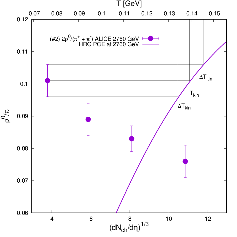
Figure 1: The $\rho^{0}/\pi$ ratio as function of centrality (experimental data) and temperature (theoretical curves). The determination of the kinetic freeze-out temperature and its uncertainty is illustrated. The lower horizontal axis belongs to the measured data points, the upper, temperature axis belongs to the model calculations. The value of the measured data point is projected onto the theoretical curve and the corresponding temperature is read off.

The calculations were started from the initial values listed in Table 2.

Table 2: The initial temperature, chemical potentials and strangeness saturation parameters for the model calculations. In the case of ALICE, the values we utilized the parametrization published in Ref. Andronic et al. (2018)., for STAR, the parameters are given in Ref. Adamczyk et al. (2017). For wider centrality bins (e.g. $0-10\%$ bin), we calculate the error-weighted-average from the centrality bins that cover the needed one. In the cases of tighter bins we use the same values in each bin which value was given for the covering one (e.g. $60-70\%$ and $70-80\%$ bins have the same value from the $60-80\%$ centrality bin).

ALICE ($\sqrt{s_{\textmd{NN}}}=$ 2760 GeV)
centrality	$T_{\textmd{chem}}$ [GeV]	$\mu_{B}$ [GeV]	$\mu_{S}$ [GeV]	$\gamma_{S}$
$-$	0.159	0	0	1
STAR ($\sqrt{s_{\textmd{NN}}}=$ 200 GeV)
centrality	$T_{\textmd{chem}}$ [GeV]	$\mu_{B}$ [GeV]	$\mu_{S}$ [GeV]	$\gamma_{S}$
0-5%	0.1643	0.0284	0.0056	0.93
5-10%	0.1635	0.0284	0.0050	0.95
10-20%	0.1624	0.0277	0.0059	0.94
20-30%	0.1639	0.0274	0.0064	0.90
30-40%	0.1616	0.0239	0.0060	0.90
40-50%	0.1623	0.0229	0.0058	0.84
50-60%	0.1623	0.0229	0.0058	0.84
60-70%	0.1613	0.0182	0.0054	0.76
70-80%	0.1613	0.0182	0.0054	0.76
0-10%	0.1639	0.0284	0.0053	0.94
10-40%	0.1627	0.0264	0.0061	0.91
40-60%	0.1623	0.0229	0.0058	0.84
60-80%	0.1613	0.0182	0.0054	0.76

In the case of STAR the $T_{\textmd{chem}}$, chemical freeze-out temperatures, differ slightly from what one would obtain from the parametrisation in Andronic et al. (2018). We decided to use the given values because they do not differ significantly from the one given by the parametrisation. On the other hand, we utilised the parametrisation for the higher energy Adamczyk et al. (2017). The obtained $\mu_{h}(T)$ are employed to determine the number densities for each resonance species, as functions of $T$. Based on this, temperature dependence of the particle ratios can be predicted. This is illustrated in Fig. 1. on the example of $\rho^{0}/\pi$ ratio. The solid line in the Figure shows the calculated ratio as the function of temperature.

The calculations were done for every particle species for which measurements are available in the literature (see Tab. 1.), and the temperature-dependent ratios were compared to the corresponding experimental data point(s). This comparison is illustrated in Fig. 1. Notice the two horizontal scales on this plot: the bottom one corresponds to the data points, and the top scale is the temperature of the model calculations. The kinetic freeze-out temperature can be determined by projecting the experimental values onto the theoretical curve, as illustrated with one data point in the Figure. The uncertainties can be determined in the same way.

It could happen that a data point or a measured uncertainty does not intercept with the calculated curve within the considered temperature range. In such cases we give an estimate, i.e., we do not give the kinetic freeze out temperature value with an uncertainty but we give the range where the experimental uncertainty interval overlaps with the theoretical curve.

IV Results

The first ratio—$\rho^{0}/\pi$—was illustrated in Fig. 1. Qualitatively, we observe that as collisions become more central, the data points correspond to a lower temperature. The temperatures for all data points will be summarised later.

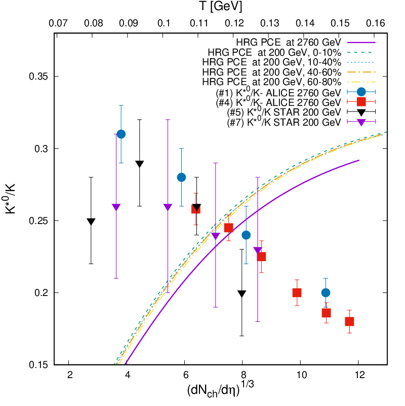
Figure 2: The $K^{*}/K$ ratios as functions of centrality (experimental data points) and temperature (theoretical curves). Solid curve stands for calculation for Pb+Pb collisions at $\sqrt{s_{NN}}=2.76$ TeV (all centralities). Non-solid curves correspond to different centralities of Au+Au collisions at $\sqrt{s_{NN}}=200$ GeV (and practically overlap). For the data points, the numbers in brackets refer to data set numbers from Table 1.

Model calculations and other measured data points are superimposed in Figs. 2-5. In Fig. 2, we plot the data on $K^{*}/K$ ratio for different centralities of Au+Au collisions at $\sqrt{s_{\textmd{NN}}}=200$ GeV as well as Pb+Pb collisions at $\sqrt{s_{\textmd{NN}}}=2.76$ TeV. At RHIC energies, the theoretical curves for different centralities are practically on top of each other, while there is always only one theoretical curve for ALICE, since the chemical potentials for all centralities are identical. The rough qualitative picture is again that more central data indicate lower kinetic freeze-out temperature. Nevertheless, the most peripheral ALICE data points do not match the theoretical curves anywhere and we can only find an overlap of the theoretical value with a fraction of the measured uncertainty interval.

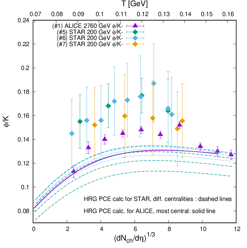
Figure 3: Same at Fig. 2, but for the $\phi/K$ ratios. Solid curve for Pb+Pb at $\sqrt{s_{NN}}=2.76$ TeV (all centralities). Non-solid curves for Au+Au at $\sqrt{s_{NN}}=200$ GeV from central (top curves) to peripheral (bottom curves) collisions. For the data points, the numbers in brackets refer to data set numbers from Table 1.

The disagreement of theory to experiment becomes most severe for the $\phi/K$ ratio, plotted in Fig. 3. Practically all measured data points are above the theoretical curve. In the present scheme, only the mesons from the pseudo-scalar octet are treated as stable. Hence, in spite of its rather long lifetime, $\phi$ is treated as an unstable resonance. This means that it stays always in equilibrium with its decay products, notably with $K$ and $\bar{K}$. To stay consistently in framework of the PCE model, we do not modify this assumption. Note that the calculated ratio barely changes all the way down to the temperature $T=110$ MeV. For the collisions at the LHC, the ratios in central collisions are reproduced by PCE calculations for a large interval of temperatures. However, the measured ratios for more peripheral collisions overshoot the theoretical values. This also seems to be the case for all measured values at $\sqrt{s_{\textmd{NN}}}=200$ GeV. It indicates some non-equilibrium mechanism beyond the current PCE treatment, possibly the decoupling of $\phi$ from the tower of $K$ and $\bar{K}$ resonances.

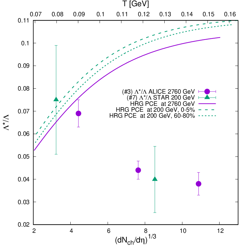
Figure 4: Same at Fig. 2, but for the $\Lambda^{*}/\Lambda$. Solid curve for Pb+Pb at $\sqrt{s_{NN}}=2.76$ TeV (all centralities). Dashed and dotted lines for Au+Au collisions at $\sqrt{s_{NN}}=200$ GeV, centrality 0–5% and 60-80%, respectively. For the data points, the numbers in brackets refer to data set numbers from Table 1.

An opposite situation appears for the $\Lambda^{*}/\Lambda$ ratio, see Fig. 4. The overall trend seems similar as for the $K^{*}/K$: data for more central collisions appear to correspond to a lower temperature than those from peripheral collisions. However, the actual measured values are so low that the calculation would have to be brought to temperature below 70 MeV in order to reproduce central and mid-central data, but the fireball would have broken up before it would cool down so much. For two data points from $\sqrt{s_{\textmd{NN}}}=200$ GeV we can find an overlap with the theoretical curves only cthanks to the large error bars.

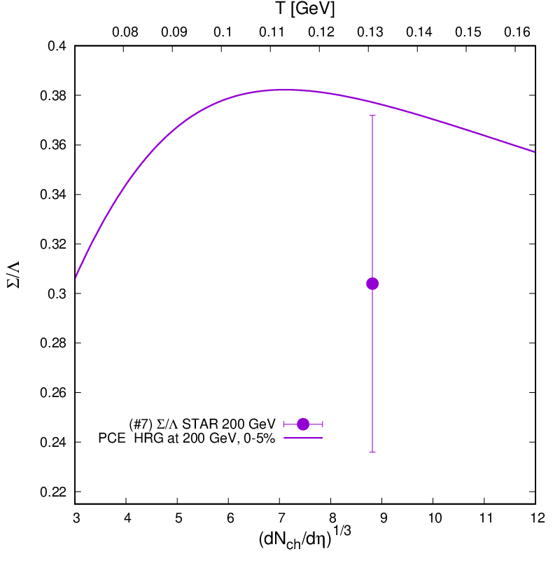
Figure 5: Same at Fig. 2, but for the $\Sigma^{*}/\Lambda$ ratio. Data point and calculation for Au+Au collisions at $\sqrt{s_{NN}}=200$ GeV, centrality 0–5%.

There is only one data point measured for the $\Sigma^{*}/\Lambda$ ratio, as seen in Fig. 5. Even though the actual data point is below the theoretical curve, there is an overlap of the uncertainty interval with a portion of the curve, owing to the large measured error bars.

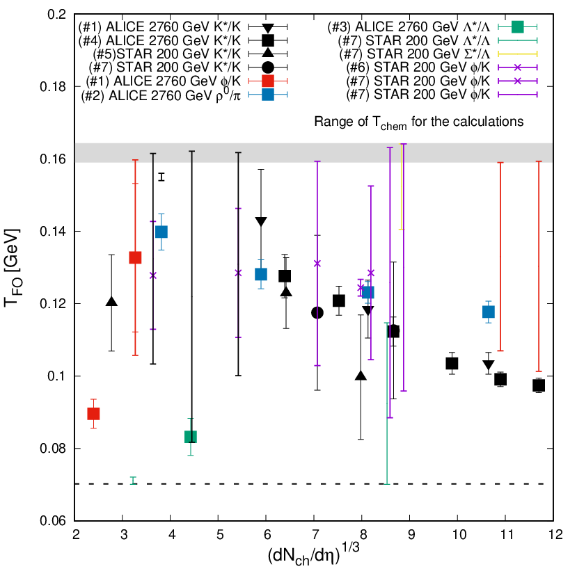
Figure 6: The freeze-out temperatures resulting from the measured values of resonance ratios. For the data points, the numbers in brackets refer to data set numbers from Table 1.

We summarize our results for the extracted temperatures in Fig. 6, for all the ratios included in our analyses. In cases where we had the overlap of the measured value with the theory, we show the resulting temperature. If there was just a partial overlap with the uncertainty interval, we only show bars in the plot. Due to their large abundance, the dominant behaviour seems to be set by the $K^{*}/K$ data, which generally decrease when moving to more central collisions. The $\rho/\pi$ ratios seem to fall into the same temperature dependence, with some difference for the most central collisions. There, $\rho/\pi$ indicates a temperature higher by 15 MeV than the $K^{*}/K$ ratio. The ratios of $\phi/K$ and $\Lambda^{*}/\Lambda$ either fall out of this temperature dependence or are connected with too large uncertainty intervals to make any reasonable conclusions.

V Conclusions

A part of the motivation for this study was to check if and how the resonance production indicates the same freeze-out parameters as the single-particle $p_{t}$ spectra. An analysis if the $p_{t}$ spectra, which lead to the kinetic freeze-out temperatures for different centralities of Pb+Pb collisions at $\sqrt{s_{\textmd{NN}}}=2.76$ TeV Melo and Tomášik (2016) yielded results that are consistent with those of $K^{*}/K$ ratios. This is plotted in Fig. 7.

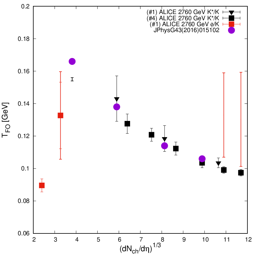
Figure 7: The freeze-out temperatures from the $K^{*}/K$ ratios from Pb+Pb collisions at $\sqrt{s_{\textmd{NN}}}=2.76$ TeV, compared with the kinetic freeze-out temperatures obtained from fitting $p_{t}$ spectra of pions, (anti)protons, and kaons Melo and Tomášik (2016).

Nevertheless, the partial chemical equilibrium is but one special scenario, which can be assumed for the evolution of the fireball after the chemical freeze-out.

The disagreement of the $\phi/K$ ratio best points to the shortcomings of the model setup. While $\phi$ is rather stable on the time scale of the hadronic fireball lifetime, the PCE treats it as unstable to such an extent, that it remains in equilibrium with its decay products. Accounting for $\phi$ as stable particle would possibly increase its abundance.

This may be the strongest hint to the non-equilibrium behaviour of higher-mass states and possible rescattering of their daughter particles Knospe et al. (2016). Such an mechanism would also include the scenario with a short hadron phase Mazeliauskas and Vislavicius (2020).

Another shortcoming of the PCE model is the assumption of isentropic evolution. It remains to be studied in the future, how this assumption can be relaxed and what impact on the results it would have.