On Data-Driven Log-Optimal Portfolio:
A Sliding Window Approach

Abstract

In this paper, we propose a data-driven sliding window approach to solve a log-optimal portfolio problem. In contrast to many of the existing papers, this approach leads to a trading strategy with time-varying portfolio weights rather than fixed constant weights. We show, by conducting various empirical studies, that the approach possesses a superior trading performance to the classical log-optimal portfolio in the sense of having a higher cumulative rate of returns.

and

1 Introduction

The take-off point for this paper is the so-called log-optimal portfolio, which is any portfolio that maximizes the Expected Logarithmic Growth (ELG) of a trader’s wealth. This ELG maximization idea was originated from Kelly jr (1956) to solve repeated coin-flipping gambling problems. Since then, various ramifications and extensions along this line are studied extensively; e.g., see Algoet and Cover (1988); Rotando and Thorp (1992); Cover and Thomas (2006); Thorp (2006). Specifically, the objective for solving the classical ELG problem is to seek a portfolio with weight $K$ of its account value that maximizes the ELG at the terminal stage. Some good and bad properties are studied in MacLean et al. (2010). A rather comprehensive survey of the Kelly-based approach can be found in MacLean et al. (2011) and the references therein. While many of the existing papers contributed to Kelly’s problem and its application to stock trading; e.g., see Rotando and Thorp (1992); Algoet and Cover (1988); Cover and Thomas (2006); Lo et al. (2018); Kuhn and Luenberger (2010); Thorp (2006); Hsieh et al. (2016), the resulting optimal weights $K$ are typically time-invariant.

According to Cover and Thomas (2006); Cornuejols and Tütüncü (2006), it is known that if the returns are independent and identically distributed (IID) and known perfectly to the trader, then the constant weight $K$ is optimal. However, in practice, the returns are typically neither IID nor perfectly known to the trader; see Fama (2021) and Luenberger (2013). To this end, various approaches are proposed to solve the log-optimal portfolio problem by relaxing the IID assumptions; e.g., see Cover (1991) for proposing a universal portfolio with unknown return distributions and Rujeerapaiboon et al. (2018, 2016); Sun and Boyd (2018) for solving various robust Kelly optimal portfolio problems. In contrast, this paper, under somewhat weak assumptions on returns, aimed at studying the data-driven log-optimal portfolio problem via a sliding window approach. Unlike many of the papers mentioned above that considering a portfolio with a fixed constant weight; see Algoet and Cover (1988); Thorp (2006); Nekrasov (2014); Hsieh et al. (2018); Hsieh (2021, 2022), our approach leads to a time-varying portfolio weight, which generalizes the case with a fixed constant weight. To close this brief introduction, we also mention some related work here; e.g., see Park and Irwin (2007) for a good survey of the profitability of technical analysis, Wu et al. (2022) for an interesting application of using Kelly-based approach in options trading, Hsieh (2020) for analyzing log-optimal fraction using Taylor-based approximation approach.

1.1 Plans for Section to Follow

In Section 2, we provide some preliminaries and formulate a data-driven log-optimal portfolio problem in a discrete-time setting. Then, in Section 3, a sliding window algorithm is provided to solve the portfolio problem. Subsequently, in Section 4, with the sliding window approach, we provide various empirical studies using historical stock price data. Lastly, in Section 5, some concluding remarks and future research directions are discussed.

2 Problem Formulation

Fix an integer $N>1$. For stages $k=0,1,\dots,N-1$, we consider a trader who is forming a portfolio consisting of $m\geq 2$ assets. If an asset is riskless, its return is deterministic and is treated as a degenerate random variable with value $X(k)=r\geq 0$ for all $k$ with probability one. Alternatively, if Asset $i$ is a stock whose price at time $k$ is $S_{i}(k)>0$, then its return is

$$X_{i}(k)=\frac{S_{i}(k+1)-S_{i}(k)}{S_{i}(k)}.$$

In the sequel, we assume that the return vectors

$$X(k):=\left[X_{1}(k)\;X_{2}(k)\;\cdots\;X_{m}(k)\right]^{T}.$$

The return vector $X(k)$ is drawn according to an unknown but identically distributed distribution which is supported on $J$ distinct points. For $k=0,1,\dots,N-1$, the corresponding joint probability mass function can be estimated by

$$P(X_{1}(k)=x_{1}^{j},\dots,X_{m}(k)=x_{m}^{j})=P(X(k)=x^{j})=p_{j}$$

for $j=1,2,\dots,J$ with $p_{j}\geq 0$ and $\sum_{j=1}^{J}p_{j}=1.$ We also assume that the returns satisfy $X_{\min,i}\leq X_{i}(k)\leq X_{\max,i}$ with known bounds above and with $X_{\max,i}$ being finite and $X_{\min,i}>-1$.

2.1 Portfolio Weight and Account Value Dynamics

For $k=0,1,\dots$, let $V(k)$ be the trader’s account value at stage $k$. Now, for $i=1,2,\dots,m$, take $0\leq K_{i}\leq 1,$ which represents a weight of the portfolio allocated to the $i$th asset. In the sequel, we require that the trade is long-only and cash-financed. Specifically, using a shorthand notation $K:=[K_{1}\;K_{2}\;\cdots\;K_{m}]^{T},$ we require that the weight must satisfy the classical unit simplex constraint; i.e.,

$$K\in\mathcal{K}:=\left\{K\in\mathbb{R}^{m}:K_{i}\geq 0\text{ for all }\ i,\ \sum_{i=1}^{m}K_{i}=1\right\}.$$

Now, at stage $k=0,$ we begin with the initial account value $V(0):=V_{0}>0$. The associated account value dynamics can be described as the following stochastic recursive equation

$$V(k+1) =(1+K^{T}X(k))V(k).$$

The per-period log-return is defined as

$$g(k):=\log\frac{V(k+1)}{V(k)}$$

which is used as the objective of the maximization in the sections to follow.

2.2 Data-Driven Log-Optimal Portfolio Problem

To incorporate with available data, we modify the problem and consider the data-driven log-optimal portfolio problem:

$$\max_{K\in\mathcal{K}}\ \mathbb{E}\left[g(k)\right] =\max_{K\in\mathcal{K}}\ \mathbb{E}[\ \log(1+K^{T}X(k))\ ]$$

$$=\max_{K\in\mathcal{K}}\ \sum_{j=1}^{J}p_{j}\log(1+K^{T}x^{j}).$$ (1)

The problem above is readily verified as a concave program; i.e., a maximization problem with a concave objective and a convex constraint set $\mathcal{K}$; see Boyd and Vandenberghe (2004). In this paper, we will use a modeling language called CVXPY (using Python language); see Diamond and Boyd (2016). CVXPY enable us to solve the problem in a very efficient manner.

Remark 2.1

To close this section, it is worth mentioning that, unlike many of the existing papers in solving log-optimal portfolio using fixed constant weight, our approach seeks to find a portfolio weight $K\in\mathcal{K}$ by solving the latest optimal portfolio problem with sliding window sizes $M\geq 1$. The resulting optimal weight $K\in\mathcal{K}$ will be applied to the successive stage $k+1$. Then we “slide” the window and resolve the problem. The procedure is repeated until the terminal stage.

3 Sliding Window Algorithm

In this section, we are ready to introduce our sliding window approach aimed at solving the data-driven log-optimal portfolio problem stated in Section 2. Specifically, for each $k=0,1,\dots$, we rebalance our portfolio using a sliding window with sizes $M$ days to obtain the latest optimal weight.

Using $s_{i}(k)$ to denote the realized prices for Asset $i$ at stage $k$, the associated realized returns $x_{i}(k)$ satisfy

$$x_{i}(k):=\frac{s_{i}(k+1)-s_{i}(k)}{s_{i}(k)}$$ (2)

for $i=1,2,\dots,m$. Let

$$x(k):=\left[x_{1}(k)\;x_{2}(k)\;\cdots\;x_{m}(k)\right]^{T}.$$

Now sitting at $k=k_{0}$, the sliding window approach is aimed at obtaining an optimal $K^{*}$ that will be applied to the next stage $k_{0}+1$. To this end, we proceed as follows. We begin by selecting a collection of realized returns $\{x(j)\}_{j=k_{0}-M}^{k_{0}-1}$, which is obtained in $M$ past stages. Subsequently, we solve the maximization problem to obtain the $K^{*}$. The detailed algorithm is summarized below.

Algorithm 1 Data-Driven Sliding Window Algorithm

1:Consider $m\geq 2$ assets, stock prices $\{s_{i}(j)\}_{k=0}^{N-1}$ for $i=1,2,\dots,m$, and sliding window size $M$.

2:Optimal portfolio weight $K^{*}$ for each stage

3:Compute realized returns $\{x_{i}(k)\}_{k=0}^{N-1}$ with $x_{i}(k)$ defined in Equation (2).

4:if $k\geq M$ then

5:     Choose $\{x(j)\}_{j=k-M}^{k-1}$ from $\{x(k)\}_{k=0}^{N-1}$ with joint probability $p_{j}:=1/M$ for all $j=k-M,\dots,k-1$.

6:     Solve the maximization problem

$$\max_{K\in\mathcal{K}}\ \frac{1}{M}\sum\limits_{j=k-M}^{k-1}\ \log(1+K^{T}x(j)).$$

7:     Having obtained optimal $K^{*}(k):=K^{*}$, we apply it at stage $k+1$. Set $k=k+1$ then back to Step 2.

8:end if

4 Empirical Studies

To illustrate our sliding window approach, two empirical studies are considered: The first one is a three-asset portfolio using daily prices and the second one is the same portfolio using the flipped upside down prices. Consistent with the existing literature; e.g., Bodie et al. (2018), to compare the trading performance, some typical metrics are used as follows.

4.1 Performance Metrics

For $k=0,1,\dots,N-1$, the first performance metric to be used in the analysis to follow is the portfolio realized return in period $k$. That is,

$$R^{p}(k):=\frac{V(k+1)-V(k)}{V(k)}.$$

The (realized) cumulative return up to stage $k=N$ is given by $(V(N)-V(0))/V(0)$ and the log-growth rate is the logarithm of the realized cumulative return; i.e., $\log(V(N)/V(0))$. The excess return denoted

$$R^{p}(k):=R^{p}(k)-r_{f}$$

where $r_{f}$ is the risk-free rate. The realized (per-period) Sharpe ratio, denoted by $SR$, of the portfolio is the average of the excess returns $\overline{R^{p}}$ over the standard deviation of the excess returns $\sigma$; i.e.,

$$SR:=\frac{\overline{R^{p}}-r_{f}}{\sigma}$$

and the N-period realized Sharpe ratio can be approximated by $\sqrt{N}\cdot SR$; see Lo (2002). Lastly, other than standard deviation, to scrutinize the downside risks over multi-period trading performance, we include the maximum percentage drawdown as an alternative risk metric; i.e.,

$$d^{*}:=\max_{0\leq\ell<k\leq N}\frac{V(\ell)-V(k)}{V(\ell)}.$$

Lastly, we also report the running times of the sliding window approach. For example, with $m=3$ assets, we generate $10,000$ of sample paths using the historical daily price data with window sizes $M=10$. On a laptop with $2.5$ GHz with $4$GB RAM, the data-driven log-optimal problem can be solved about $3.18$ seconds, which is in the same scale of solving classical log-optimal portfolio.

Example 4.1 (Three Assets Portfolio)

Consider a portfolio consisting of three underlying assets: The first asset is Vanguard Total World Stock (Ticker: VT), the second asset is Vanguard Total Bond Market ETF (Ticker: BND), and the third asset is Vanguard Total International Bond ETF (Ticker: BNDX). Assuming $r_{f}:=0$ and a two-year duration from February 14, 2018 to February 14, 2020, we solve the log-optimal portfolio problem to obtain the optimal weight $K^{*}$. The corresponding prices are shown in Figure 1. Beginning with an initial account value $V(0)=\$1$, we compare our sliding window approach with the classical log-optimal portfolio.

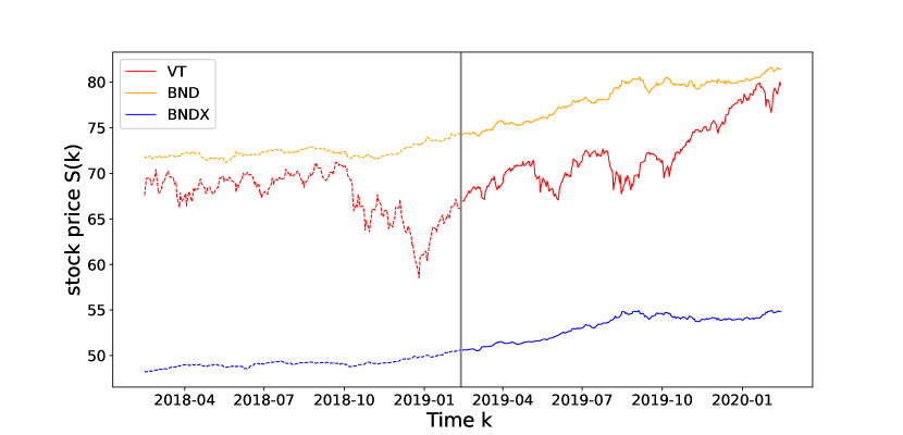
Figure 1: Daily Stock Prices for VT, BND, and BNDX

Specifically, to obtain the classical log-optimal portfolio $K^{*}$, we solve Problem (1) for the first year of the data from August 14, 2018 to February 13, 2019. The corresponding optimal $K^{*}$ is given by $K^{*}=e_{3}:=[0\;0\;1]^{T},$ which suggests that one should invest all of available funds on BNDX. The out-of-sample performance metrics under classical log-optimal portfolio are summarized in Table 1. The corresponding account value trajectory is shown in Figure 2 with a bold solid line in black color. From the figure, we see that at the terminal stage, $V(N)\approx 1.0849$ with a maximum percentage drawdown about $d^{*}=2.21\%$.

Table 1: Performance Metrics under Classical Log-Optimal Portfolio

Classical log-optimal portfolio $K^{*}$
Maximum percentage drawdown $d^{*}$	$2.21$%
Cumulative rate of return $\frac{V(N)-V_{0}}{V_{0}}$	$8.49$%
Realized Log-Growth $\log\frac{V(N)}{V(0)}$	$8.15$%
volatility (Annualized) $\sigma$	$2.85$%
Sharpe ratio $\sqrt{N}\cdot SR$	$2.87$
Running Times (secs)	$3.17$

4.2 Log-Optimal Portfolio with Sliding Window Approach

With various window sizes $M=5,10,30,60,$ and $100$, we calculate the log-optimal portfolio weight $K^{*}(k)$ via the sliding window approach mentioned in Section 3. Having obtained $K^{*}(k)$, we then implement it on the next trading stage $k+1$; see Figure 2 for an illustration. According to the figure, we find that a relatively small $M$; e.g., $M=5$ or $M=10$, appears to lead to a higher cumulative return. Instead of investing on BNDX only as suggested by the classical log-optimal portfolio with a constant weight, the sliding window approach yields a time-varying weight; e.g., see Figure 3.

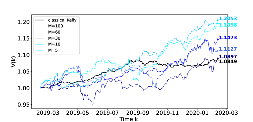
Figure 2: Classical Log-Optimal Portfolio Versus Sliding Window Approach with Sizes $M=5,10,30,60,$ and $100$

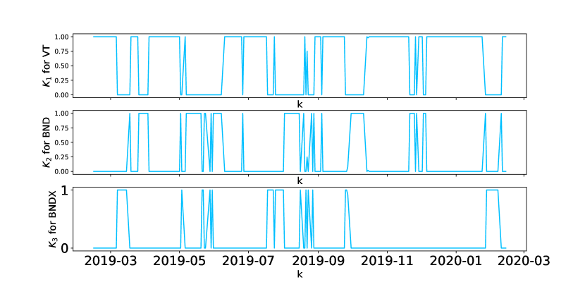
Figure 3: Time-Varying Portfolio Weights $K(k)$ with size $M=10$ for the Three-Asset Portfolio

Various performance metrics are summarized in Table 2. It is worth noting that one can view the window size $M$ as a new design variable in the following sense: One seeks an optimal size $M^{*}$ that gives the largest return or lowest volatility. In this example, $M=10$ appears to be the best choice in terms of various performance metrics such as Sharpe ratio.

Table 2: Performance Metrics Under Sliding Window Approach

Log-Optimal Portfolio with Sliding Window Approach
Sliding window sizes $M$	$100$	$60$	$30$	$10$	$5$
Maximum percentage drawdown $d^{*}$	$6.39\%$	$4.99\%$	$6.44\%$	$2.35\%$	$6.27\%$
Cumulative rate of return $\frac{V(N)-V_{0}}{V_{0}}$	$8.80\%$	$14.53\%$	$11.29\%$	$20.55\%$	$19.40\%$
Realized Log-Growth $\log\frac{V(N)}{V(0)}$	$8.43\%$	$13.56\%$	$10.70\%$	$18.69\%$	$17.73\%$
Volatility (Annualized) $\sigma$	$8.36\%$	$7.70\%$	$8.30\%$	$6.30\%$	$7.54\%$
Sharpe ratio (Annualized) $\sqrt{N}\cdot SR$	$1.050$	$1.801$	$1.331$	$2.998$	$2.389$
Running Times (secs)	$3.614$	$6.277$	$3.325$	$3.187$	$2.880$

Example 4.2 (A Hypothetical Case)

Here we consider the same setting but with the hypothetical flipped upside-down prices, which corresponds to a bear market situation. Using the sliding window algorithm in Section 3 to test for the flipped upside-down case. Figure 4 shows the hypothetical prices of all these three assets (VT, BND, BNDX) from February 14, 2018 to February 14, 2020. To obtain a classical log-optimal portfolio $K^{*}$, we solve the log-optimal portfolio problem for one year ago from February 14, 2018 to February 13, 2019, and apply optimal $K^{*}$ into the next year from February 14, 2019 to February 14, 2020. In this case, corresponding log-optimal portfolio $K^{*}$ is given by $K^{*}=e_{3}:=[0\;0\;1]^{T},$ which suggests one should invest all of available money on asset BNDX. The corresponding account value trajectory is shown in Figure 5 in a bold solid line with black color. Other performance metrics are summarized in Table 3.

Table 3: Performance Metrics of Classical Log-Optimal Portfolio (Hypothetical Case)

Classical log-optimal portfolio $K^{*}$
Maximum percentage drawdown $d^{*}$	$4.81\%$
Cumulative rate of return $\frac{V(N)-V_{0}}{V_{0}}$	$-4.73\%$
Realized Log-Growth $\log\frac{V(N)}{V(0)}$	$-4.84\%$
Volatility (Annualized) $\sigma$	$1.89\%$
Sharpe ratio $\sqrt{N}\cdot SR$	$-2.56$
Running Times (secs)	$4.36$

Similar to Example 4.1, we again implement Algorithm 1 with various window sizes $M=5,10,30,60$, and $100$ days. The corresponding account value trajectories are shown in Figure 5. Consistent with our theory, the resulting strategy yields a time-varying portfolio weight; see Figure 6 for an example of this fact with size $M=10$.

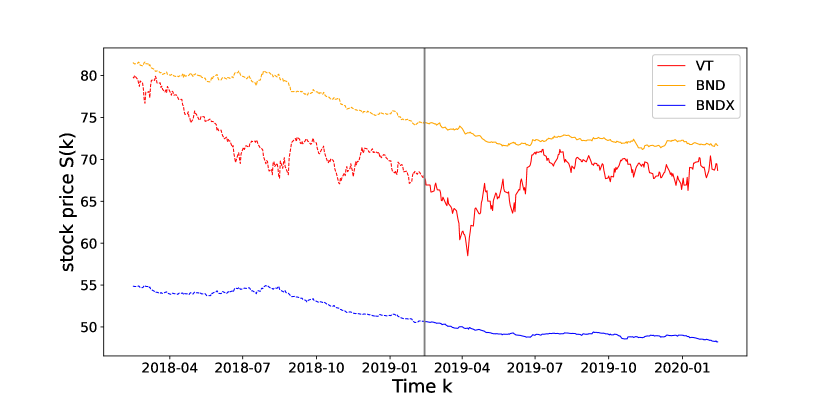
Figure 4: Hypothetical Daily Stock Prices for VT, BND, and BNDX

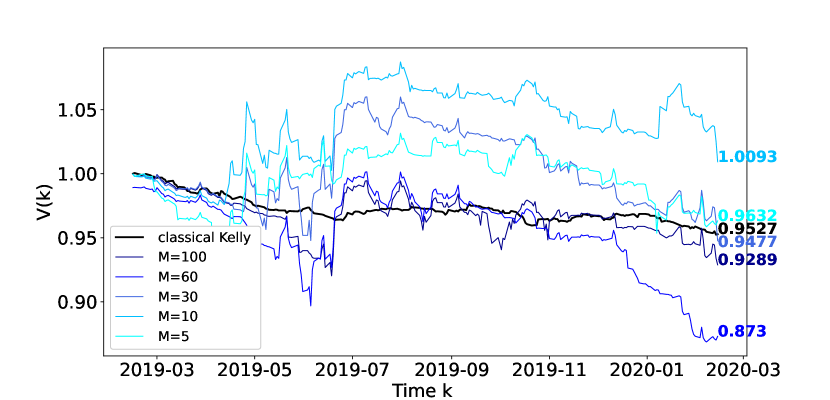
Figure 5: Classical Log-Optimal Portfolio Versus Sliding Window Approach with Sizes $M=5,10,30,60,$ and $100$ (Hypothetical Case)

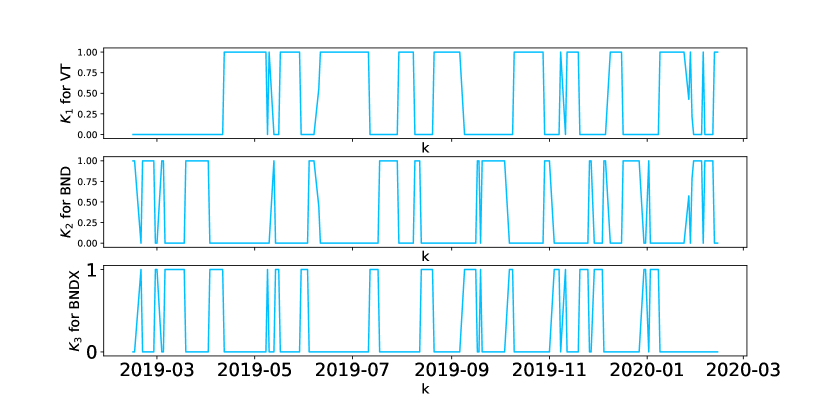
Figure 6: Time-Varying Portfolio Weights $K(k)$ with size $M=10$ (Hypothetical Case)

Even if in this (hypothetical) bear market, the sliding window approach appears to maintain the account value without falling too much. In Table 4, we see that the annualized rate of return in $M=10$ is even surprisingly positive.

Table 4: Performance Metrics Under Sliding Window Approach (Hypothetical Case)

Log-Optimal Portfolio with Sliding Window Approach
Sliding window sizes $M$	$100$	$60$	$30$	$10$	$5$
Maximum percentage drawdown $d^{*}$	$7.96\%$	$13.27\%$	$10.60\%$	$7.16\%$	$7.56\%$
Cumulative rate of return $\frac{V(N)-V_{0}}{V_{0}}$	$-7.08\%$	$-11.75\%$	$-5.20\%$	$0.97\%$	$-3.64\%$
Realized Log-Growth $\log\frac{V(N)}{V(0)}$	$-7.34\%$	$-12.49\%$	$-5.34\%$	$0.97\%$	$-3.71\%$
Volatility (Annualized) $\sigma$	$8.36\%$	$8.81\%$	$10.28\%$	$9.62\%$	$9.97\%$
Sharpe ratio (Annualized) $\sqrt{N}\cdot SR$	$-0.858$	$-1.375$	$-0.468$	$0.148$	$-0.322$
Running Times (secs)	$4.826$	$4.087$	$3.909$	$3.580$	$3.431$

5 Concluding Remarks

In this paper, we studied a sliding window approach for solving a data-driven log-optimal portfolio problem. In contrast to the classical log-optimal portfolio with a constant weight, our approach leads to a time-varying weight, which generalizes the classical case. We show, by example, that our approach may be potentially superior to that with classical log-optimal portfolio in terms of the cumulative account value. To close this brief conclusion section, we provide two possible research directions.

Optimal Window Sizes $M$. As mentioned previously in Section 4, the window sizes $M$ can be viewed as a new design variable. Hence, determining an “optimal” size would be of interest to pursue further. It is also worth mentioning that the optimization using a sliding window approach with applying the resulting optimal weights to the next trading day is indeed closely related to the idea of model predictive control; e.g., see Mayne et al. (2000) and Rawlings et al. (2017). Hence, pursuing this direction might be also fruitful.

Computational Complexity Issues. While we solve a data-driven log-optimal portfolio problem via a sliding window approach and report corresponding running times for the algorithm, we did not address the computational complexity of the proposed algorithm. Hence, it would be of great interest to analyze the time computational complexities.

References

- Algoet and Cover (1988) Algoet, P.H. and Cover, T.M. (1988). Asymptotic Optimality and Asymptotic Equipartition Properties of Log-Optimum Investment. The Annals of Probability, 16(2), 876–898.
- Bodie et al. (2018) Bodie, Z., Kane, A., and Marcus, A. (2018). Investments. McGraw Hill.
- Boyd and Vandenberghe (2004) Boyd, S. and Vandenberghe, L. (2004). Convex Optimization. Cambridge University Press.
- Cornuejols and Tütüncü (2006) Cornuejols, G. and Tütüncü, R. (2006). Optimization Methods in Finance. Cambridge University Press.
- Cover (1991) Cover, T.M. (1991). Universal Portfolios. Mathematical Finance, 1(1), 1–29.
- Cover and Thomas (2006) Cover, T.M. and Thomas, J.A. (2006). Elements of Information Theory. Wiley-Interscience.
- Diamond and Boyd (2016) Diamond, S. and Boyd, S. (2016). CVXPY: A Python-embedded modeling language for convex optimization. Journal of Machine Learning Research, 17(83), 1–5.
- Fama (2021) Fama, E.F. (2021). Market Efficiency, Long-Term Returns, and Behavioral Finance. University of Chicago Press.
- Hsieh (2020) Hsieh, C.H. (2020). On Feedback Control in Kelly Betting: An Approximation Approach. In 2020 IEEE Conference on Control Technology and Applications (CCTA), 903–908.
- Hsieh (2021) Hsieh, C.H. (2021). Necessary and Sufficient Conditions for Frequency-Based Kelly Optimal Portfolio. IEEE Control Systems Letters, 5(1), 349–354.
- Hsieh (2022) Hsieh, C.H. (2022). Generalization of Affine Feedback Stock Trading Results to Include Stop-Loss Orders. Automatica, 136, 110051.
- Hsieh et al. (2016) Hsieh, C.H., Barmish, B.R., and Gubner, J.A. (2016). Kelly Betting Can Be Too Conservative. In Proceedings of the IEEE Conference on Decision and Control (CDC), 3695–3701.
- Hsieh et al. (2018) Hsieh, C.H., Gubner, J.A., and Barmish, B.R. (2018). Rebalancing Frequency Considerations for Kelly-Optimal Stock Portfolios in a Control-Theoretic Framework. In Proceedings of the IEEE Conference on Decision and Control (CDC), 5820–5825.
- Kelly jr (1956) Kelly jr, J. (1956). A New Interpretation of Information Rate. The Bell System Technical Journal.
- Kuhn and Luenberger (2010) Kuhn, D. and Luenberger, D.G. (2010). Analysis of the Rebalancing Frequency in Log-Optimal Portfolio Selection. Quantitative Finance, 10(2), 221–234.
- Lo (2002) Lo, A.W. (2002). The Statistics of Sharpe Ratios. Financial Analysts Journal, 58(4), 36–52.
- Lo et al. (2018) Lo, A.W., Orr, H.A., and Zhang, R. (2018). The Growth of Relative Wealth and The Kelly Criterion. Journal of Bioeconomics, 20(1), 49–67.
- Luenberger (2013) Luenberger, D.G. (2013). Investment Science. Oxford university press.
- MacLean et al. (2010) MacLean, L.C., Thorp, E.O., and Ziemba, W.T. (2010). Good and Bad Properties of the Kelly Criterion. Risk, 20(2), 1.
- MacLean et al. (2011) MacLean, L.C., Thorp, E.O., and Ziemba, W.T. (2011). The Kelly Capital Growth Investment Criterion: Theory and Practice. World Scientific.
- Mayne et al. (2000) Mayne, D.Q., Rawlings, J.B., Rao, C.V., and Scokaert, P.O. (2000). Constrained model predictive control: Stability and optimality. Automatica, 36(6), 789–814.
- Nekrasov (2014) Nekrasov, V. (2014). Kelly Criterion for Multivariate Portfolios: A Model-Free Approach. Available at SSRN 2259133.
- Park and Irwin (2007) Park, C.H. and Irwin, S.H. (2007). What do we know about the profitability of technical analysis? Journal of Economic surveys, 21(4), 786–826.
- Rawlings et al. (2017) Rawlings, J.B., Mayne, D.Q., and Diehl, M. (2017). Model Predictive Control: Theory, Computation, and Design, volume 2. Nob Hill Publishing.
- Rotando and Thorp (1992) Rotando, L.M. and Thorp, E.O. (1992). The Kelly Criterion and the Stock Market. The American Mathematical Monthly, 99(10), 922–931.
- Rujeerapaiboon et al. (2018) Rujeerapaiboon, N., Barmish, B.R., and Kuhn, D. (2018). On risk reduction in kelly betting using the conservative expected value. In Proceedings of the IEEE conference on decision and control (CDC), 5801–5806.
- Rujeerapaiboon et al. (2016) Rujeerapaiboon, N., Kuhn, D., and Wiesemann, W. (2016). Robust Growth-Optimal Portfolios. Management Science, 62(7), 2090–2109.
- Sun and Boyd (2018) Sun, Q. and Boyd, S. (2018). Distributional Robust Kelly Gambling. arXiv preprint arXiv:1812.10371.
- Thorp (2006) Thorp, E.O. (2006). The Kelly Criterion in Blackjack Sports Betting, and The Stock Market. Handbook of Asset and Liability Management: Theory and Methodology, 1, 385.
- Wu et al. (2022) Wu, M.E., Syu, J.H., and Chen, C.M. (2022). Kelly-Based Options Trading Strategies on Settlement Date via Supervised Learning Algorithms. Computational Economics.