Data-Driven optimal shrinkage of singular values under high-dimensional noise with separable covariance structure with application

Abstract.

We develop a data-driven optimal shrinkage algorithm for matrix denoising in the presence of high-dimensional noise with a separable covariance structure; that is, the noise is colored and dependent across samples. The algorithm, coined extended OptShrink (eOptShrink) depends on the asymptotic behavior of singular values and singular vectors of the random matrix associated with the noisy data. Based on the developed theory, including the sticking property of non-outlier singular values and delocalization of the non-outlier singular vectors associated with weak signals with a convergence rate, and the spectral behavior of outlier singular values and vectors, we develop three estimators, each of these has its own interest. First, we design a novel rank estimator, based on which we provide an estimator for the spectral distribution of the pure noise matrix, and hence the optimal shrinker called eOptShrink. In this algorithm we do not need to estimate the separable covariance structure of the noise. A theoretical guarantee of these estimators with a convergence rate is given. On the application side, in addition to a series of numerical simulations with a comparison with various state-of-the-art optimal shrinkage algorithms, we apply eOptShrink to extract maternal and fetal electrocardiograms from the single channel trans-abdominal maternal electrocardiogram.

Keywords: matrix denoising; random matrix; high dimensional noise noise; spike model; separable covariance.

1. Introduction

We are interested in denoising a $p\times n$ signal-plus-noise data matrix $\widetilde{S}$ formed by aligning $n\in\mathbb{N}$ samples of dimension $p\in\mathbb{N}$, which is modeled by

(1) $$\widetilde{S}=S+Z=\sum_{i=1}^{r}d_{i}\mathbf{u}_{i}\mathbf{v}_{i}^{\top}+Z\in\mathbb{R}^{p\times n},$$

where $Z$ is a noise-only random matrix that may have some dependence structure, $S$ is a low-rank signal matrix with the singular value decomposition (SVD) $\sum_{i=1}^{r}d_{i}\mathbf{u}_{i}\mathbf{v}_{i}^{\top}$, where $r\geq 1$ is assumed to be small compared with $p$ and $n$, $\mathbf{u}_{i}\in\mathbb{R}^{p}$ and $\mathbf{v}_{i}\in\mathbb{R}^{n}$ are left and right singular vectors prescribing the signal, and $d_{i}>0$ are the associated singular values describing “signal strength” that may depend on $n$. We focus on the high dimensional setup; that is $p=p(n)$ and $p/n\to\beta\in(0,\infty)$ when $n\to\infty$. The setting is considered as a generalization of the traditional high dimensional spiked model [4, 5, 7]. It has been shown in [11] that under this high dimensional setup, if the empirical distribution of singular values from $Z$ converges to a non-random compactly supported probability measure, the top singular values of $\widetilde{S}$ and associated left and right singular vectors are all biased from those of $S$. These biases converge to a closed form depending on the D-transform [11] and the Stieltjes transform [56] of the limiting singular value distribution of the noise only matrix $Z$. Moreover, we have a phase transition when the signal strength $d_{i}$ exceeds a critical value, which is usually called the BBP (Baik-Ben Arous-Pèchè) phase transition named after the authors of [6]. Therefore, unlike the traditional SVD truncation scheme [27], when applying SVD to recover $S$ from $\widetilde{S}$ under the large $p$ and large $n$ set-up, we need to handle these bias. A celebrated optimal weighting approach that is later called the optimal shrinkage (OS) method [43, 47, 25] for recovering $S$ from $\widetilde{S}$ by SVD has been actively studied in the last decade. The idea of OS is selecting a proper nonlinear function $\varphi:[0,\infty)\rightarrow[0,\infty)$ and denoise the matrix by

(2) $$\widehat{S}_{\varphi}=\sum_{i=1}^{p\wedge n}\varphi(\widetilde{\lambda}_{i})\widetilde{\bm{\xi}}_{i}\widetilde{\bm{\zeta}}_{i}^{\top},$$

where ${\widetilde{\lambda}_{1}}\geq{\widetilde{\lambda}_{2}}\geq\cdots\geq{\widetilde{\lambda}_{p\wedge n}}\geq 0$, are common eigenvalues of $\widetilde{S}\widetilde{S}^{\top}$ and $\widetilde{S}^{\top}\widetilde{S}$ and $\{\widetilde{\bm{\xi}}_{i}\}$ and $\{\widetilde{\bm{\zeta}}_{i}\}$ are the left and right singular vectors of $\widetilde{S}$ respectively. Such a $\varphi$ is called a shrinker. By choosing a proper loss function $L_{n}$ that comparing $\widehat{S}_{\varphi}$ and $S$, the optimal shrinker $\varphi^{*}$ is defined as $\varphi^{*}:=\operatorname*{arg\,min}_{\varphi}\lim_{n\to\infty}L_{n}(\widehat{S}_{\phi},S)$. The close form of the optimal shrinker when $L_{n}$ is the Frobenius norm loss is derived in [40] (See Proposition 2.6 below), which requires that the empirical spectral distribution (ESD) of $Z$ asymptotically converges to a non-random compactly supported probability measure, so that the derivative of the D-transform of this measure is $-\infty$ at the right most edge of the compact support, and a critical delocalization conjecture of singular vectors. A matrix denoising algorithm named OptShrink is provided in [40] by approximating the D-transform with respect to the truncated singular value distribution of $\widetilde{S}$ assuming the knowledge of rank. OptShrink is very general, but to our knowledge, it is challenging to directly apply it to real-world problems, unless some assumptions are imposed.

Consider the white noise as a special example; that is, $Z=X$, where the entries of $X$ are i.i.d. with zero mean, variance $\sigma^{2}/n$ with $\sigma>0$, and finite fourth moment. Under such setup, asymptotically the ESD of $ZZ^{\top}$ follows the Marchenko-Pastur (MP) law [39], and in [25], the optimal shrinker $\varphi^{*}$ under various loss functions are derived using the closed form of the rightmost bulk edge $\lambda_{+}$, and $\varphi^{*}$ are determined solely by $\widetilde{\lambda}_{i}$, $\sigma$ and $\beta$. This OS approach under the white noise assumption (called TRAD hereafter) has been widely applied; for example, the fetal electrocardiogram (fECG) extraction problem from the trans-abdominal maternal ECG (ta-mECG) [50], ECG T wave quality evaluation [51], otoacoustic emission signal denoising [38], stimulation artifact removal from the intracranial electroencephalogram (EEG) [1] and cardiogenic artifact removal from the EEG [13].

We illustrate how to apply OS to one of these signal processing challenges. See Figure 1 for the fECG extraction problem. The ta-mECG recorded from the mother’s abdomen during pregnancy is shown in Figure 1(a). It is truncated into pieces indicated by the red boxes, and the truncated pieces are aligned according to the maternal R peaks. The fetal R peaks are labeled blue crosses. The associated data matrix $\widetilde{S}$ is shown in Figure 1(b), where the maternal ECG (mECG) is viewed as the signal, saved as the matrix $S$, and the fECG and inevitable noise are jointly viewed as the noise, saved as the matrix $Z$. The results of TRAD, indicated by $\widehat{S}$, are shown in red curves in Figure 1(c), which is the recovered mECG after denoise. In 1(d), we show $S-\widehat{S}$, which is the recovered fECG. The mECG and fECG have been well decomposed, and we can better visualize the fetal R peaks in Figure 1(d), while there are visible poorly recovered parts indicated by the black box, which is zoomed in in Figure 1(e). We refer readers to [50] for details, a literature review for relevant algorithms, and its clinical application.

While we have successfully applied TRAD to several applications, the white noise assumption is too strong. For example, physiologically the fECG (the noise) should not be white, and the noises among different samples should not be independent. See Figure 1(f) for an illustration of the nontrivial covariance structure of the fECG. Thus, the ESD of $ZZ^{\top}$ may not follow the MP law asymptotically, and the performance of TRAD may be suboptimal. Another common resource of the non-white noise is the application of various filters; that is, even if we assume the noise is white, the commonly applied filters could destroy the white structure. Therefore, a modification of the white noise model and TRAD to handle more complicated noise is needed. In this paper, we focus on noise with the separable covariance structure [45]:

(3) $$Z=A^{1/2}XB^{1/2}\,,$$

where the entries of $X$ are i.i.d. with zero mean and mild moment conditions that will be specified later, and $A$ and $B$ are respectively $p\times p$ and $n\times n$ deterministic positive-definite matrices that describe the colorness and dependence structure of noise, respectively. A random matrix satisfying the separable covariance structure has been studied and applied to many problems, like spatiotemporal analysis, wireless communication and several recent applications [21, 28, 26, 20]. When $B=I_{n}$, it is known that the ESD of $ZZ^{\top}$ converges to the deformed MP law [39], and the distribution of the largest eigenvalue follows the Tracy-Widom law [52, 53], or commonly referred to as the edge universality. The edge universality has been proved for $A=I_{p}$ [29, 46] and for general $A$ [22, 41, 8, 33, 17, 32] under various moment assumptions on the entries for $X$. For the sample singular vectors, the delocalization [32, 42] and ergodicity [12] have been constructed. When the general separable covariance structure is assumed, the convergence of the ESD to a limiting law is shown in [45, 55, 59], the edge universality and delocalization of eigenvectors is established in [17, 58], and the local law (local estimates of the resolvents or the Green’s functions) of $ZZ^{\top}$ is recently proved in [57, 58].

Based on the above established results under various random matrix assumptions, efforts have been devoted to design matrix denoising algorithms when the noise satisfies the separable covariance model. The special $B=I$ is discussed in [36] and the general $B$ is discussed in [37], where the author proposes to apply the whitening technique before applying TRAD; that is, perform TRAD on the whitened matrix $\widehat{A}^{-1/2}\widetilde{S}\widehat{B}^{-1/2}$, where $\widehat{A}$ and $\widehat{B}$ are the estimated $A$ and $B$ respectively. This approach works well when $A$ and $B$ can be accurately estimated; for example, when both $A$ and $B$ are diagonal. A fast numerical algorithm for $\lambda_{+}$ and the Stieltjes transform is available [34] when $Z=A^{1/2}XB^{1/2}$ and the asymptotic spectral distribution of $A$ and $B$ can be accurately estimated. In [19], if the upper bound of $r$ is known, $d_{i}$’s are distinct and several assumptions about the asymptotic ESD of $Z$ hold, a hard thresholding method named ScreeNOT is defined as

(4) $$\widehat{S}_{\texttt{SN}}=\sum_{i=1}^{p\wedge n}\sqrt{\widetilde{\lambda}_{i}}\mathbbm{1}(\widetilde{\lambda}_{i}>\vartheta)\widetilde{\bm{\xi}}_{i}\widetilde{\bm{\zeta}}_{i}^{\top},$$

where $\vartheta\geq 0$ is the hard threshold evaluated by the Steiltjes transform of the estimated ESD of $Z$ via imputation, and the case $Z=A^{1/2}X$ is discussed for the theoretical guarantee.

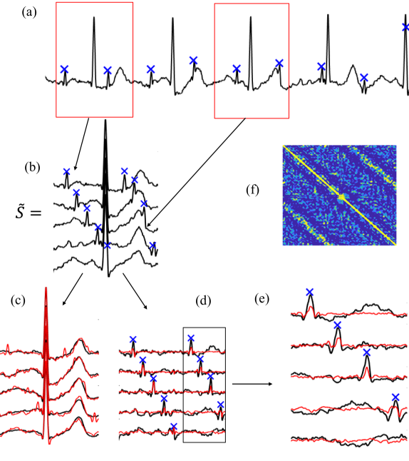
Figure 1. An illustration of extracting fECG from the ta-mECG shown in (a), where the fetal R peaks labeled by experts are marked as blue crosses. (b) is the data matrix including the pieces truncated from the ta-mECG and aligned by the maternal R peaks. The results of TRAD and our eOptShrink (both with the operator norm) as the estimated mECG are shown as red and black curves shown in (c) respectively. By subtracting the estimated mECG from the ta-mECG, we obtain the estimated fECG shown in (d). The mECG estimation error could be visualized in the estimated fECG indicated by the black box, zoomed in in (e). The covariance structure of the fECG as noise is shown in (f).

Inspired by the success and limitation of existing methods and its broad application in data science, the focus of this paper is proposing a novel matrix denoisng algorithm that is practical for denoising noisy data matrix for real world data analysis. The algorithm can be viewed as an extension of OptShrink [40], and we coin it extended OptShrink (eOptShrink). Our contributions are multifold. First, we extend the results in [9] and derive asymptotic behavior of the outlier singular values and the associated biased singular vectors of the noisy data matrix $\widetilde{S}=S+A^{1/2}XB^{1/2}$, including the BBP phase transition, the sticking properties of non-outlier singular values, and the delocalization of the non-outlier singular vectors, where the convergence rate is established. We point out that our results are in the same vine as those for deformed Wigner matrix [30, 31], deformed rectangular matrix [11, 15] and spiked covariance matrices [44, 12, 18, 16], but not yet been established for our setup to our best knowledge. Recall that the delocalization is an essential conjecture needed for OptShrink [40]. Second, based on the developed theorems, we propose a fully data-driven OS algorithm based on these results, which is composed of two novel ingredients, each of which has its own interest. The first ingredient is a novel data-driven rank estimation from $\widetilde{S}$, which is essential for OptShrink and ScreeNOT. The second ingredient is a novel approach to estimate the spectral density distribution of $Z$, which is based on an accurate recovery of the singular values of $Z$ from those of $\widetilde{S}$ that are deviated by signals. With these two ingredients, we can construct a more accurate estimate of the Steiltjes transform and D-transform compared to using the existing imputation [19] and truncation [40] approaches. We also extend OptShrink [40] to cover various loss functions other than the Frobenius norm. Numerically, we evaluate the developed theory and algorithm and compare it with existing algorithms [40, 19] from different aspects in both simulated datasets and a real-world ta-mECG database. Overall, eOptShrink outperforms other algorithms.

NOTATION: For any random variable ${X}$, denote ${\widetilde{X}}$ as the perturbed ${X}$, and ${\widehat{X}}$ as the estimator of ${X}$. $C$ denotes a generic positive constant, whose value may change from one line to another. For sequences $\{a_{n}\}$ and $\{b_{n}\}$ indexed by $n$, $a_{n}=\operatorname{O}(b_{n})$ means that $|a_{n}|\leq C|b_{n}|$ for some constant $C>0$ as $n\to\infty$ and $a_{n}=\operatorname{o}(b_{n})$ means that $|a_{n}|\leq c_{n}|b_{n}|$ for some positive sequence $c_{n}\downarrow 0$ as $n\to\infty$. We also use $a_{n}\lesssim b_{n}$ if $a_{n}=\operatorname{O}(b_{n})$, $|a_{n}|\ll|b_{n}|$ if $a_{n}=\operatorname{o}(b_{n})$, and $a_{n}\asymp b_{n}$ if $a_{n}=\operatorname{O}(b_{n})$ and $b_{n}=\operatorname{O}(a_{n})$. For a matrix $M$, $\|M\|$ means its operator norm and we may abuse the notation and write $M=\operatorname{O}(a)$ if $\|M\|=\operatorname{O}(a)$. $I$ is reserved for the identity matrix of any dimension. For $a,b\in\mathbb{R}$, $a\vee b$ and $a\wedge b$ mean the maximal and minimal value of $a$ and $b$ respectively. We reserve $E+i\eta$ to indicate a point in $\mathbb{C}^{+}$, the upper half plan of $\mathbb{C}$. See Tables S.1 and S.2 for a list of notations.

2. Preliminaries

2.1. Background on random matrix theory

To study singular values and singular vectors of $Z$ and $\widetilde{S}$, we need to review the following results about Green functions and Stieltjes transforms. The Stieltjes transform of a probability measure, $\nu$ is $m_{\nu}(z):=\int{\frac{1}{\lambda-z}}d\nu(\lambda)$, where $z\in\mathbb{C}^{+}$. For an $n\times n$ symmetric matrix $H$, the ESD of $H$ is defined as $\pi_{H}:=\frac{1}{n}\sum_{i=1}^{n}\delta_{\ell_{i}}$, where $\ell_{1}\geq\ell_{2}\geq\cdots\geq\ell_{n}$ are the eigenvalues of $H$ and $\delta$ means the Dirac delta measure. Denote the common eigenvalues of $ZZ^{\top}$ and $Z^{\top}Z$ (respectively $\widetilde{S}\widetilde{S}^{\top}$ and $\widetilde{S}^{\top}\widetilde{S}$) by $\{\lambda_{i}\}_{i=1}^{p\wedge n}$ (respectively $\{\widetilde{\lambda}_{i}\}_{i=1}^{p\wedge n}$). For $z\in\mathbb{C}^{+},$ denote the Green functions of $ZZ^{\top}$ and $Z^{\top}Z$ as

(5) $$\mathcal{G}_{1}(z):=(ZZ^{\top}-z{I_{p}})^{-1}\ \mbox{ and }\ \mathcal{G}_{2}(z):=(Z^{\top}Z-z{I_{n}})^{-1}$$

respectively. The Stieltjes transforms of ESDs of $ZZ^{\top}$ and $Z^{\top}Z$ are formulated respectively by the Green functions $\mathcal{G}_{1}(z)$ and $\mathcal{G}_{2}(z)$ via

(6) $$m_{1}(z):=\frac{1}{p}\text{Tr}\mathcal{G}_{1}(z)\ \mbox{ and }\ m_{2}(z):=\frac{1}{n}\text{Tr}\mathcal{G}_{2}(z).$$

Denote $\beta_{n}:=\frac{p}{n}.$ By a direct calculation, we have the relationship $m_{2}(z)=-\frac{1-\beta_{n}}{z}+\beta_{n}m_{1}(z)$. Similarly, we denote the Green functions of $\widetilde{S}\widetilde{S}^{\top}$ and $\widetilde{S}^{\top}\widetilde{S}$ as

(7) $$\mathcal{\widetilde{G}}_{1}(z):=(\widetilde{S}\widetilde{S}^{\top}-z{I_{p}})^{-1}\ \mbox{ and }\ \mathcal{\widetilde{G}}_{2}(z):=(\widetilde{S}^{\top}\widetilde{S}-z{I_{n}})^{-1}$$

respectively and the Stieltjes transforms of ESDs of $\widetilde{S}\widetilde{S}^{\top}$ and $\widetilde{S}^{\top}\widetilde{S}$ as

(8) $$\widetilde{m}_{1}(z):=\frac{1}{p}\text{Tr}\mathcal{\widetilde{G}}_{1}(z)\ \mbox{ and }\ \widetilde{m}_{2}(z):=\frac{1}{n}\text{Tr}\mathcal{\widetilde{G}}_{2}(z)\,.$$

Next we summarize the asymptotic behavior of $m_{1}(z)$ and $m_{2}(z)$. From [45], if $\beta_{n}\to\beta\in(0,\infty)$ and $\pi_{A}$ and $\pi_{B}$ converge to nonrandom probability distributions $\rho_{A}$ and $\rho_{B}$ with compact supports when $n\to\infty$, and the entries $X$ are independent with mean 0 and the same variance, then almost surely $\pi_{ZZ^{\top}}$ and $\pi_{Z^{\top}Z}$ converge to deterministic distributions with compact supports. Define $(\mathsf{m}_{1c}(z),\mathsf{m}_{2c}(z))\in\mathbb{C}^{+}\times\mathbb{C}^{+}$ as the unique solution to the following system of self-consistent equations

$$\mathsf{m}_{1c}(z)=\beta_{n}\int\frac{x}{-z[1+x\mathsf{m}_{2c}(z)]}\pi_{A}(dx)\ \mbox{ and }\ \mathsf{m}_{2c}(z)=\int\frac{x}{-z[1+x\mathsf{m}_{1c}(z)]}\pi_{B}(dx)\,.$$

From the above equations, if we define a function $f$ on $\mathbb{C}^{+}\times\mathbb{C}^{+}$ by $f(z,m):=-m+\int\frac{x}{-z+x\beta_{n}\int\frac{t}{1+tm}\pi_{A}(dt)}\pi_{B}(dx)$, then $\mathsf{m}_{2c}(z)$ can be characterized as the unique solution so that $f(z,\mathsf{m}_{2c}(z))=0$ for $z\in\mathbb{C}^{+}$ [45]. Moreover, $\mathsf{m}_{1c}(z)$ and $\mathsf{m}_{2c}(z)$ are the Stieltjes transforms of the densities $\varrho_{1c}$ and $\varrho_{2c}$ since

(9) $$\varrho_{1c}(E)=\lim_{\eta\downarrow 0}\frac{1}{\pi}\operatorname{Im}\,\mathsf{m}_{1c}(E+i\eta)\ \mbox{ and }\ \varrho_{2c}(E)=\lim_{\eta\downarrow 0}\frac{1}{\pi}\operatorname{Im}\,\mathsf{m}_{2c}(E+i\eta)\,,$$

where $z=E+i\eta\in\mathbb{C}^{+}$. Define

(10) $$m_{1c}(z):=\int\frac{1}{-z[1+x\mathsf{m}_{2c}(z)]}\pi_{A}(dx)\ \mbox{ and }\ m_{2c}(z):=\int\frac{1}{-z[1+x\mathsf{m}_{1c}(z)]}\pi_{B}(dx)\,.$$

It has been known that when $n\to\infty$, $m_{1c}(z)-m_{1}(z)$ and $m_{2c}(z)-m_{2}(z)$ converge to zero uniformly with respect to $z$. See [58, Theorem 3.6] and [18, Theorem S.3.9] for details. Again, by letting $\eta\downarrow 0$, we obtain their corresponding probability measures with the inverse formula

(11) $$\rho_{1c}(E)=\lim_{\eta\downarrow 0}\frac{1}{\pi}\operatorname{Im}\,m_{1c}(E+i\eta)\ \mbox{ and }\ \rho_{2c}(E)=\lim_{\eta\downarrow 0}\frac{1}{\pi}\operatorname{Im}\,m_{2c}(E+i\eta)\,.$$

We recall the following lemma from Section 3 of [14].

Lemma 2.1.

Let $A$ and $B$ be deterministic symmetric matrices with eigenvalues $\sigma_{1}^{a}\geq\sigma_{2}^{a}\geq\ldots\geq\sigma_{p}^{a}$ and $\sigma_{1}^{b}\geq\sigma_{2}^{b}\geq\ldots\geq\sigma_{n}^{b}$ respectively and satisfy

(12) $$\sigma_{1}^{a}\vee\sigma_{1}^{b}\leq\tau^{-1}\ \mbox{ and }\ \pi_{A}([0,\tau])\vee\pi_{B}([0,\tau])\leq 1-\tau.$$

Then the densities $\rho_{1c}$, $\rho_{2c}$, $\varrho_{1c}$ and $\varrho_{2c}$ all have the same support on $(0,\infty)$, which is a union of finite intervals $\bigcup_{k=1}^{L}[e_{2k},e_{2k-1}]\cap(0,\infty)$, where $L\in\mathbb{N}$ depends only on $\pi_{A}$ and $\pi_{B}$ and $e_{1}>e_{2}>\ldots>e_{2L}$. Moreover, $(x,m)=(e_{k},\mathsf{m}_{2c}(e_{k}))$ are the real solutions of the equations $f(x,m)=0$ and $\frac{\partial f}{\partial m}(x,m)=0$. Finally, $e_{1}$ is bounded, $\mathsf{m}_{1c}(e_{1})\in(-(\max_{j}\sigma_{j}^{b})^{-1},0)$ and $\mathsf{m}_{2c}(e_{1})\in(-(\max_{i}\sigma_{i}^{a})^{-1},0)$.

We call $e_{k}$ the spectral edges. In this paper, we focus on the rightmost edge $\lambda_{+}:=e_{1}$. $[e_{2L},2_{1}]$ could be viewed as the “spectral spreading” of the noise, and intuitively, the signal should be sufficiently strong compared with $\lambda_{+}$ “in some way” so that the signal can be observed. This “strength” will be precisely described below. For $z\in\mathbb{C}^{+}$, we denote the $D$-transform of $\rho_{1c}$ as

(13) $$\mathcal{T}(z):=zm_{1c}(z)m_{2c}(z)\,.$$

See the free probability theory, e.g., [11, Section 2.5], for more details. $m_{1c}$ and $m_{2c}$ can be extended to $x>\lambda_{+}$ so that

(14) $$m_{1c}(x)=\int_{0}^{\lambda_{+}}\frac{\rho_{1c}(t)}{t-x}dt\ \mbox{ and }\ m_{2c}(x)=\int_{0}^{\lambda_{+}}\frac{\rho_{2c}(t)}{t-x}dt\,.$$

Thus, when $x>\lambda_{+}$, $m_{1c}(x)$, $m_{2c}(x)$ and $\mathcal{T}(x)$ are well-defined. Moreover, by a direct calculation, both $m_{1c}(x)$ and $m_{2c}(x)$ are negative and monotonically increasing and $\mathcal{T}(x)$ is monotonically decreasing, such that $m_{1c}(x)$, $m_{2c}(x)$ and $\mathcal{T}(x)$ are invertible. This is the key property we count on to study the signal deformation under the high dimensional noise. We denote the $j$-th classical location of the probability density $\rho_{2c}$, where $j=1,\ldots,n$, as

(15) $$\gamma_{j}:=\sup_{x}\left\{\int_{x}^{+\infty}\rho_{2c}(x)dx>\frac{j-1}{n}\right\}\,.$$

In particular, we have $\gamma_{1}=\lambda_{+}$.

2.2. Model Assumption

We impose assumptions on the data matrix model (1).

Definition 2.2.

(Bounded support condition). A random matrix $X=[x_{ij}]_{i=1,\ldots,p,j=1,\ldots,n}$ has a bounded support $\phi_{n}>0$ if $\max_{i,j}|x_{i,j}|\leq\phi_{n}$, where $\phi_{n}$ is a deterministic parameter and satisfies $\phi_{n}=n^{2/a-1/2}$ for some constant $a>4$.

This bounded support assumption is introduced to simplify the discussion, and it can be easily removed. Recall that for a random matrix $X$ whose entries are i.i.d. and have at least $4+\epsilon$ moments, it can be reduced to a random matrix with bounded support with probability $1-o(1)$ using the truncation, centralization, and rescaling [3, Section 4.3.2]. Since we do not assume the entries of $X$ are identically distributed, the means and variances of the truncated entries may be different.

Assumption 2.3.

Fix a small constant $0<\tau<1$. We need the following assumptions for the model (1):

• (Assumption on $x_{ij}$). Suppose $X$ has a bounded support $\phi_{n}$,

  (16) $$\max_{i,j}\left|\mathbb{E}x_{ij}\right|\leq n^{-2-\tau}\ \mbox{ and }\ \max_{i,j}\left|\mathbb{E}|x_{ij}|^{2}-n^{-1}\right|\leq n^{-2-\tau}\,.$$

  Further, we assume that there exists a constant $C_{4}>0$ such that

  (17) $$\mathbb{E}|\sqrt{n}x_{ij}|^{4}\leq C_{4}.$$

• (Assumptions on $p/n$). $p=p(n)$ satisfies

  (18) $$\tau<\frac{p}{n}<\tau^{-1}\,.$$

• (Assumption on $A$ and $B$). Assume $A$ and $B$ are deterministic symmetric matrices with eigendecompositions

  (19) $$A=Q^{a}\Sigma^{a}(Q^{a})^{\top}\ \mbox{ and }\ B=Q^{b}\Sigma^{b}(Q^{b})^{\top}$$

  respectively, where $\Sigma^{a}=\textup{diag}(\sigma_{1}^{a},\ldots,\sigma_{p}^{a})$, $\Sigma^{b}=\textup{diag}(\sigma_{1}^{b},\ldots,\sigma_{n}^{b})$, $\sigma_{1}^{a}\geq\sigma_{2}^{a}\geq\ldots\geq\sigma_{p}^{a}$, $\sigma_{1}^{b}\geq\sigma_{2}^{b}\geq\ldots\geq\sigma_{n}^{b},$ $Q^{a}=({\bf q}^{a}_{1},\cdots,{\bf q}^{a}_{p})\in O(p)$ and $Q^{b}=({\bf q}^{b}_{1},\cdots,{\bf q}^{b}_{n})\in O(n)$. We assume that

  (20) $$1+\mathsf{m}_{1c}(\lambda_{+})\sigma_{1}^{b}\geq\tau\ \mbox{ and }\ 1+\mathsf{m}_{2c}(\lambda_{+})\sigma_{1}^{a}\geq\tau\,.$$

  Moreover, for all sufficiently large $n$, we assume (12) holds.

• (Assumption on the signal strength). We assume

  (21) $$d_{1}\geq d_{2}\geq\cdots\geq d_{r}>0$$

  for some $r\geq 1$. Further, we assume that $d_{i}<\tau^{-1}.$ Denote a fixed value $\alpha>0$ as

  (22) $$\alpha:=1/\sqrt{\mathcal{T}(\lambda_{+})}\,.$$

  We allow the singular values $d_{k}$ to depend on $n$ under the condition that there exists an integer $1\leq r^{+}\leq r$ such that

  (23) $$d_{k}-\alpha>\phi_{n}+n^{-1/3}\ \mbox{ for }\ 1\leq k\leq r^{+}\,.$$

• (Assumption on distribution of the singular vectors). Let $G_{\mathbf{u}}^{p}\in\mathbb{R}^{p\times r}$ and $G_{\mathbf{v}}^{n}\in\mathbb{R}^{n\times r}$ be two independent matrices with i.i.d entries distributed according to a fixed probability measure $\nu$ on $\mathbb{R}$ with mean zero and variance one, and satisfy the log-Sobolev inequality (see below). We assume that the left and right singular vectors, $\mathbf{u}_{i}\in\mathbb{R}^{p}$ and $\mathbf{v}_{i}\in\mathbb{R}^{n}$, are the $i$-th columns obtained from the Gram-Schmidt (or QR factorization) of $\frac{1}{\sqrt{n}}G_{\mathbf{u}}^{n}$ and $\frac{1}{\sqrt{n}}G_{\mathbf{v}}^{n}$ respectively.

In (iii), (20) and (12) guarantees a regular square-root behavior of the spectral densities $\rho_{1c}$ and $\rho_{2c}$ near $\lambda_{+}$ (See Lemma S.2.6) and rules out the existence of outlier eigenvalues from $ZZ^{\top}$. Therefore, it also makes sure that $\mathcal{T}(\lambda_{+})$ is well-defined so as $\alpha$ in (iv). The second condition means that the spectra of $A$ and $B$ cannot concentrate at zero. In (iv), $d_{i}$ that fulfills (23) is considered “sufficiently strong” that is associated with a “strong signal”. Below we will see that when a signal is sufficiently strong, it leads to an “outlier” in the spectrum of $\tilde{S}$, so that it is possible to study the signal. Note that not all signals lead an outlier. If $d_{i}$ does not satisfy (23), they are considered “weak” that is associated with a “weak signal”, and we will show in Theorem 3.2 that the weak signals will lead to “non-outlier” singular values of $\tilde{S}$; that is, these singular values lie within a neighborhood of order $n^{-2/3}+\phi_{n}^{2}$ of the rightmost edge of singular values of $Z$, which is related to the BBP phase transition. Hence in (23), $r^{+}$ is considered the “efficient rank” of $\widetilde{S}$. In (v), the log-Sobolev inequality implies that entries of $\mathbf{u}_{i}$ and $\mathbf{v}_{i}$ have sub-Gaussian tails, and hence nice concentration properties [2, Section 2.3.2] that we will describe in Lemma S.2.5. See Figure S.5 for an illustration of the relationship of $\mathcal{T}$, $\alpha$ and $\lambda_{+}$.

2.3. Optimal shrinkers for various loss functions

Recall the definition of asymptotic loss and optimal shrinker provided in [25, Definitions 1 and 2] .

Definition 2.4 (Asymptotic loss).

Let $\mathcal{L}:=\{L_{p,n}|p,n\in\mathbb{N}\}$ be a family of loss functions, where each $L_{p,n}:M_{p\times n}\times M_{p\times n}\rightarrow[0,\infty)$ is a loss function obeying $L_{p,n}(S,S)=0.$ Suppose $p=p(n)$ and $\lim_{n\to\infty}p(n)/n\to\beta>0$. Let $\varphi:[0,\infty)\rightarrow[0,\infty)$ be a nonlinear function and consider $\widehat{S}_{\varphi}$ to be the singular shinkage estimate (2). When $\lim_{n\rightarrow\infty}L_{p,n}$ exists, we define the asymptotic loss of the shrinker $\varphi$ with respect to $L_{p,n}$ with the signal $\mathbf{d}=(d_{1},\cdots,d_{r})$ as $L_{\infty}(\varphi|\mathbf{d})=\lim_{n\rightarrow\infty}L_{p,n}(S,\widehat{S}_{\varphi})$, where $S$ is defined in (1).

Definition 2.5 (Optimal shrinker).

Let $L_{\infty}$ and $\varphi$ as defined in Definition 2.4. If a shrinker $\varphi^{*}$ has an asymptotic loss that satisfies $L_{\infty}(\varphi^{*}|\mathbf{d})\leq L_{\infty}(\varphi|\mathbf{d})$ for any other shrinker $\varphi$, any $r\geq 1$, and any $\mathbf{d}\in\mathbb{R}^{r},$ then we say that $\varphi^{*}$ is unique asymptotically admissible (or simply “optimal”) for the loss family $\mathcal{L}$ and that class of shrinkers.

In [25, Sections IV. A and C], the optimal shrinkers under different loss functions were computed. When the loss function is the operator norm, the optimal shrinker was proved to be $\varphi_{i}=d_{i}$ when $p=n$ in [25, Section IV.B]. Later in [35, Lemma 5.1], it is shown that $\varphi_{i}=d_{i}\sqrt{\frac{a_{1,i}\wedge a_{2,i}}{a_{1,i}\vee a_{2,i}}}$ when $p\neq n$, where $a_{1,i}:=\lim_{n\to\infty}\langle\mathbf{u}_{i},\widetilde{\bm{\xi}}_{i}\rangle^{2}$ and $a_{2,i}:=\lim_{n\to\infty}\langle\mathbf{v}_{i},\widetilde{\bm{\zeta}}_{i}\rangle^{2}$. We list the results here for readers’ convenience. Denote $\varphi_{i}:=\varphi^{*}(\widetilde{\lambda}_{i})$.

Proposition 2.6 ([25, 35]).

When $d_{i}\geq\alpha$, the optimal shrinker is $\varphi_{i}=d_{i}\sqrt{a_{1,i}a_{2,i}}$, $\varphi_{i}=d_{i}\sqrt{\frac{a_{1,i}\wedge a_{2,i}}{a_{1,i}\vee a_{2,i}}}$ and $\varphi_{i}=d_{i}\big{(}\sqrt{a_{1,i}a_{2,i}}-\sqrt{(1-a_{1,i})(1-a_{2,i})}\ \big{)}$ when the Frobenius norm, operator norm and nuclear norm are considered in the loss function respectively. When $d_{i}<\alpha$, for any loss function, we have $\varphi_{i}=0$.

With Proposition 2.6, if we can estimate $d_{i}$, $a_{1,i}$ and $a_{2,i}$ using the eigenstructure of the noisy matrix $\widetilde{S}\widetilde{S}^{\top}$, we could obtain the desired optimal shrinkers. For example, as shown in [11], if the ESD of $Z$ converges almost surely weakly to a compactly supported probability measure, then when $d_{i}>\alpha$, we have that $d_{i}=\frac{1}{\sqrt{\mathcal{T}(\widetilde{\lambda}_{i})}}$, $a_{1,i}=\frac{m_{1c}(\widetilde{\lambda}_{i})}{d_{i}^{2}\mathcal{T}^{\prime}(\widetilde{\lambda}_{i})}$ and $a_{2,i}=\frac{m_{2c}(\widetilde{\lambda}_{i})}{d_{i}^{2}\mathcal{T}^{\prime}(\widetilde{\lambda}_{i})}$, based on which the optimal shrinker with respect to the Frobenius norm is derived by replacing $d_{i}\sqrt{a_{1,i}a_{2,i}}$ with the corresponding values in [40]. Moreover, as shown in [25], when the noise is white with $\sigma>0$, and $X$ have independent entries with zero mean, unit variance, and finite fourth moment, if $d_{i}>\beta^{1/4}$, we have $\widetilde{\lambda}_{i}>\sigma(1+\sqrt{\beta})$ as $n\to\infty$. Denote $y_{i}=\widetilde{\lambda}_{i}/\sigma^{2}$. We have $d_{i}=\ell_{i}$, $a_{1,i}={\frac{\ell_{i}^{4}-\beta}{\ell_{i}^{4}+\beta\ell_{i}^{2}}}$ and $a_{2,i}={\frac{\ell_{i}^{4}-\beta}{\ell_{i}^{4}+\ell_{i}^{2}}}$, where $\ell_{i}:=\frac{1}{\sqrt{2}}\sqrt{y_{i}-\beta-1+\sqrt{({y_{i}}-\beta-1)^{2}-4\beta}}.$ In this special case, when $\widetilde{\lambda}_{i}>\sigma(1+\sqrt{\beta})$, the optimal shrinker has the closed form ${\varphi}_{i}=\frac{\sigma}{y_{i}}\sqrt{(y_{i}^{2}-\beta-1)^{2}-4\beta}$, ${\varphi}_{i}=\sigma\ell_{i}$ and ${\varphi}_{i}=\frac{\sigma}{\ell_{i}^{2}y_{i}}(\ell_{i}^{4}-\beta-\sqrt{\beta}\ell_{i}y_{i})$ respectively when the Frobenius norm, operator norm, and nuclear norm respectively is considered, and when $\widetilde{\lambda}_{i}\leq\sigma(1+\sqrt{\beta})$, $\varphi_{i}=0$ for any loss function. The rank can be decided by how many $\widetilde{\lambda}_{i}>\sigma(1+\sqrt{\beta})$. If $\sigma$ is unknown, it is suggested in [24] to estimate $\sigma$ by $\check{\sigma}(\widetilde{S}):=s_{med}/\sqrt{\mu_{\beta}}$, where $s_{med}$ is a median singular value of $\widetilde{S}$ and $\mu_{\beta}$ is the median of the MP distribution. To extend OptShrink under our noise setup (3), we study the asymptotic behavior of singular values and vectors and their relation with $d_{i}$, $a_{1,i}$ and $a_{2,i}$ with a convergence rate.

3. Main Results

In this section we state the main theoretical results about the biased singular values and vectors, including the limiting behavior and the associated convergence rate. These results form the foundation of the proposed eOptShrink algorithm. To simplify the presentation of our results and their proofs, we apply the notion of stochastic domination, which is a systematic framework to state results of the form “$\xi$ is bounded by $\zeta$ with high probability up to a small power of $n$” [23].

Definition 3.1 (Stochastic domination).

Let $\xi=\left(\xi^{(n)}(u):n\in\mathbb{N},u\in U^{(n)}\right)$ and $\zeta=\left(\zeta^{(n)}(u):n\in\mathbb{N},u\in U^{(n)}\right)$ be two families of nonnegative random variables, where $U^{(n)}$ is a possibly $n$-dependent parameter set. We say $\xi$ is stochastically dominated by $\zeta$, uniformly in $u$, if for any fixed (small) $\epsilon>0$ and (large) $D>0$, $\sup_{u\in U^{(n)}}\mathbb{P}\left[\xi^{(n)}(u)>n^{\epsilon}\zeta^{(n)}(u)\right]\leq n^{-D}$ for large enough $n\geq n_{0}(\epsilon,D)$, and we shall use the notation $\xi\prec\zeta$ or $\xi=O_{\prec}(\zeta)$. Throughout this paper, the stochastic domination will always be uniform in all parameters that are not explicitly fixed, such as matrix indices, and $z$ that takes values in some compact set. Note that $n_{0}(\epsilon,D)$ may depend on quantities that are explicitly constant, such as $\tau$ in Assumption 2.3. Moreover, we say an event $\Xi$ holds with high probability if for any constant $D>0$, $\mathbb{P}(\Xi)\geq 1-n^{-D}$, when $n$ is sufficiently large.

We denote $\{\bm{\xi}_{i}\}_{i=1}^{p}$ and $\{\bm{\zeta}_{i}\}_{i=1}^{n}$ as respectively the left and right singular vectors of the noise matrix $Z$, and $\{\widetilde{\bm{\xi}}_{i}\}_{i=1}^{p}$ and $\{\widetilde{\bm{\zeta}}_{i}\}_{i=1}^{n}$ as respectively the left and right singular vectors of $\widetilde{S}$, which can be viewed as a perturbation of $Z$ by adding $S$. For $x>\alpha$, denote $\theta(x)$, $a_{1}(x)$ and $a_{2}(x)$ by

(24) $$\theta(x):=\mathcal{T}^{-1}(x^{-2}),\ a_{1}(x)=\frac{m_{1c}(\theta(x))}{x^{2}\mathcal{T}^{\prime}(\theta(x))},\ a_{2}(x)=\frac{m_{2c}(\theta(x))}{x^{2}\mathcal{T}^{\prime}(\theta(x))}\,.$$

These terms are used to estimate the signal strength $d_{i}$ and inner products of the clean and noisy left singular vectors $\langle\mathbf{u}_{i},\widetilde{\bm{\xi}}_{j}\rangle$ and clean and noisy right singular vectors $\langle\mathbf{v}_{i},\widetilde{\bm{\zeta}}_{j}\rangle$, which we will detail in the following theorems.

3.1. Results of singular values

We first state the results for singular values. Define

(25) $$\mathbb{O}_{+}=\{1,\cdots,r^{+}\}\ \mbox{ and }\ \Delta(d_{i}):=|d_{i}-\alpha|^{1/2}\,.$$

Recall that the singular values index by $\mathbb{O}_{+}$ are called outliers and others are non-outliers. The followings are our main theorems, and their proofs are postponed to the supplementary. Part of the proof of the following theorems is motivated by [58] and [18], where the focus is the covariance matrix analysis. The main difference comes from the fact that in general, the covariance model in [58, 18] cannot be directly decomposed into the summation of two independent matrices, like $S$ and $Z=A^{1/2}XB^{1/2}$ in our model, so the results cannot be directly applied. We first state the location of the outlier eigenvalues and the first a few non-outlier eigenvalues of $\widetilde{S}\widetilde{S}^{\top}$.

Theorem 3.2.

Suppose Assumption 2.3 holds. Then we have for $1\leq i\leq r^{+},$

(26) $$|\widetilde{\lambda}_{i}-\theta(d_{i})|\prec\phi_{n}\Delta^{2}(d_{i})+n^{-1/2}\Delta(d_{i})\,.$$

Furthermore, for a fixed integer $\varpi>r^{+}$, we have for $r^{+}+1\leq i\leq\varpi$,

(27) $$|\widetilde{\lambda}_{i}-\lambda_{+}|\prec n^{-2/3}+\phi_{n}^{2}\,.$$

The above theorem gives the large deviation bounds for the locations of the outliers and the top finite non-outlier eigenvalues of $\widetilde{S}\widetilde{S}^{\top}$. Consider the case when $0<d_{i}-\alpha=\Delta(d_{i})^{2}\leq n^{-1/3}+\phi_{n}$, then the right-hand side of (26) is bounded by $n^{-2/3}+\phi_{n}^{2}$, which is the same as (27). This implies the occurrence of the BBP transition [6]. Moreover, when $\phi_{n}\leq n^{-1/3}$, the right-hand side of (27) becomes $n^{-2/3}$, which means the non-outlier eigenvalues associated with weak signals follow the Tracy-Widom law [54]. Next, we study the eigenvalue sticking, which states how the non-outlier eigenvalues of $\widetilde{S}\widetilde{S}^{\top}$ “stick” to the eigenvalues of $ZZ^{\top}$.

Theorem 3.3.

Suppose Assumption 2.3 holds and

(28) $$\alpha_{+}:=\min_{1\leq i\leq r}\left|d_{i}-\alpha\right|\geq n^{\varepsilon}(\phi_{n}+n^{-1/3})$$

for a small constant $0<\varepsilon<\frac{1}{2}-\frac{2}{a}$. Fix a small constant $\tau>0$. We have

(29) $$\left|\widetilde{\lambda}_{r^{+}+i}-\lambda_{i}\right|\prec\frac{1}{n\alpha_{+}}+n^{-3/4}+i^{1/3}n^{-5/6}+n^{-1/2}\phi_{n}+i^{-2/3}n^{-1/3}\phi_{n}^{2}$$

for all $1\leq i\leq\tau n$. If either (a) $\mathbb{E}x_{ij}^{3}=0$ for all $1\leq i\leq p$ and $1\leq j\leq n$, or (b) either $A$ or $B$ is diagonal, we have a stronger bound for all $1\leq i\leq\tau n$:

(30) $$\left|\widetilde{\lambda}_{r^{+}+i}-\lambda_{i}\right|\prec\frac{1}{n\alpha_{+}}\,.$$

Theorem 3.3 establishes the large deviation bound for the non-outlier eigenvalues of $\widetilde{S}\widetilde{S}^{\top}$ with respect to the eigenvalues of $ZZ^{\top}$. The parameter $\alpha_{+}$ impacts how strongly non-outlier eigenvalues of $\widetilde{S}\widetilde{S}^{\top}$ stick to eigenvalues of $ZZ^{\top}$. When $\alpha_{+}$ is too small, we do not expect the stickness; instead, when $r>r^{+}$, the behavior of $\widetilde{\lambda}_{i}$ for $i=r^{+}+1,\ldots,r$ follows (27). On the contrary, when $\alpha_{+}\gg n^{-1/3}$ and $\phi_{n}\leq n^{-1/6}$, the right-hand side of (29) and (30) are much smaller than $n^{-2/3}$ for a fixed finite $i$.

3.2. Results of singular vectors

Next we discuss the singular vectors. We first show that when $i\notin\mathbb{O}_{+}$, the non-outlier singular vectors, $\widetilde{\bm{\xi}}_{i}$ and $\widetilde{\bm{\zeta}}_{i}$, are distributed roughly uniformly and approximately perpendicular to the space spanned by $\{\mathbf{u}_{j}\}_{j=1}^{r}$ and $\{\mathbf{v}_{j}\}_{j=1}^{r}$ respectively. This delocalization is the key step toward designing eOptShrink.

Theorem 3.4.

Suppose Assumption 2.3 holds. For $i=1,\ldots,n$, denote $\eta_{i}:=n^{-3/4}+n^{-5/6}i^{1/3}+n^{-1/2}\phi_{n}$ and $\varkappa_{i}:=i^{2/3}n^{-2/3}$. For any sufficiently small constant $c>0$ and $r^{+}+1\leq i\leq cn$, we have for $j=1,\ldots,r$,

(31) $$|\langle\mathbf{u}_{j},\widetilde{\bm{\xi}}_{i}\rangle|^{2}\vee|\langle\mathbf{v}_{j},\widetilde{\bm{\zeta}}_{i}\rangle|^{2}\prec\frac{n^{-1}+\phi_{n}^{3}+\eta_{i}\sqrt{\varkappa_{i}}}{\Delta(d_{j})^{4}+\phi_{n}^{2}+\varkappa_{i}}\,.$$

If either $A$ or $B$ is diagonal, the right hand side of (31) becomes $\frac{n^{-1}+\phi_{n}^{3}}{\Delta(d_{j})^{4}+\phi_{n}^{2}+\varkappa_{i}}$. Moreover, fix a constant $\widetilde{\tau}\in(0,1/9)$ such that $n^{\widetilde{\tau}}(\phi_{n}+n^{-1/3})\to 0$ as $n\to\infty$. If $i\in\mathbb{O}_{+}$ satisfies

(32) $$\Delta(d_{i})^{2}\leq n^{\widetilde{\tau}}(\phi_{n}+n^{-1/3})\,,$$

we have for $j=1,\ldots,r$,

(33) $$|\langle\mathbf{u}_{j},\widetilde{\bm{\xi}}_{i}\rangle|^{2}\vee|\langle\mathbf{v}_{j},\widetilde{\bm{\zeta}}_{i}\rangle|^{2}\prec n^{3\widetilde{\tau}}\left(\frac{n^{-1}+\phi_{n}^{3}+\eta_{i}\sqrt{\varkappa_{i}}}{\Delta(d_{j})^{4}+\phi_{n}^{2}+\varkappa_{i}}\right).$$

To appreciate this theorem, assume $\phi_{n}\leq n^{-1/3}$ and $d_{j}$, $1\leq j\leq r^{+}$, satisfies $d_{j}-\alpha\gtrsim 1$. Then $\widetilde{\xi}_{i}$ and $\widetilde{\zeta}_{i}$ are completely delocalized so that for all $r^{+}+1\leq i\leq n^{1/4}$, $|\langle\mathbf{u}_{j},\widetilde{\bm{\xi}}_{i}\rangle|^{2}\vee|\langle\mathbf{v}_{j},\widetilde{\bm{\zeta}}_{i}\rangle|^{2}\prec n^{-1}$. On the other hand, when $d_{j}$ is close to the threshold $\alpha$, for a fixed finite $i$ so that $\widetilde{\lambda}_{i}$ is near the edge $\lambda_{+}$, (31) gives $|\langle\mathbf{u}_{j},\widetilde{\bm{\xi}}_{i}\rangle|^{2}\vee|\langle\mathbf{v}_{j},\widetilde{\bm{\zeta}}_{i}\rangle|^{2}\prec\frac{n^{-1}}{|d_{j}-\alpha|^{2}+n^{-2/3}}$; that is, the delocalization bound changes from the optimal order $n^{-1}$ to $n^{-1/3}$ as $d_{j}$ approaches $\alpha$.

Next, we state the behavior of the “outlier” singular vectors. For any $\textbf{A}\subset\mathbb{O}_{+}$, define

(34) $$\nu_{i}(\textbf{A}):=\begin{cases}\min_{j\notin\textbf{A}}|d_{j}-d_{i}|,&\textup{ if }i\in\textbf{A},\\ \min_{j\in\textbf{A}}|d_{j}-d_{i}|,&\textup{ if }i\notin\textbf{A}\end{cases}$$

and two projections,

(35) $$\mathcal{P}_{\textbf{A}}:=\sum_{k\in\textbf{A}}\widetilde{\bm{\xi}}_{k}\widetilde{\bm{\xi}}_{k}^{\top}\ \mbox{ and }\ \mathcal{P}^{\prime}_{\textbf{A}}:=\sum_{k\in\textbf{A}}\widetilde{\bm{\zeta}}_{k}\widetilde{\bm{\zeta}}_{k}^{\top}.$$

Theorem 3.5.

Suppose Assumption 2.3 holds. Fix any $\textbf{A}\subset\mathbb{O}_{+}$, we have

(36) $$\left|\langle\mathbf{u}_{i},\mathcal{P}_{\textbf{A}}\operatorname{\mathbf{u}}_{j}\rangle-\delta_{ij}\mathbbm{1}(i\in\textbf{A})a_{1}(d_{i})\right|\vee\left|\langle\mathbf{v}_{i},\mathcal{P}^{\prime}_{\textbf{A}}\mathbf{v}_{j}\rangle-\delta_{ij}\mathbbm{1}(i\in\textbf{A})a_{2}(d_{i})\right|\prec Q(i,j,\textbf{A},n)$$

for all $i,j=1,\cdots,r$, where

$$Q(i,j,\textbf{A},n)= \,\mathbbm{1}(i\in\textbf{A},j\notin\textbf{A})\Delta(d_{i})\left[\frac{\phi_{n}}{\nu^{1/2}_{j}(\textbf{A})}+\frac{\psi_{1}(d_{j})\Delta(d_{j})}{\nu_{j}(\textbf{A})}\right]$$

$$+\mathbbm{1}(i\notin\textbf{A},j\in\textbf{A})\Delta(d_{j})\left[\frac{\phi_{n}}{\nu^{1/2}_{i}(\textbf{A})}+\frac{\psi_{1}(d_{i})\Delta(d_{i})}{\nu_{i}(\textbf{A})}\right]+\sqrt{R(i,\textbf{A})R(j,\textbf{A})}\,,$$

$R(i,\textbf{A}):=\mathbbm{1}(i\in\textbf{A})\psi_{1}(d_{i})+\mathbbm{1}(i\notin\textbf{A})\frac{\phi_{n}^{2}}{\nu_{i}(\textbf{A})}+\frac{\psi_{1}^{2}(d_{i})\Delta^{2}(d_{i})}{\nu^{2}_{i}(\textbf{A})}$ and $\psi_{1}(d_{i}):=\phi_{n}+\frac{n^{-1/2}}{\Delta(d_{i})}$.

Theorem 3.5 establishes the large deviation bound for the relationship between singular vectors of $\widetilde{S}$ and $S$, which is the foundation of our proposed eOptShrink algoritthm. Take the left singular vectors $\mathbf{u}_{i}$ and $\widetilde{\xi}_{i}$ for example. Let $\textbf{A}=\{i\}$. From (36) we have that

(37) $$|\langle\mathbf{u}_{i},\widetilde{\xi}_{i}\rangle|^{2}=a_{1}(d_{i})+\operatorname{O}_{\prec}\left(\psi_{1}(d_{i})+\frac{\psi_{1}^{2}(d_{i})\Delta^{2}(d_{i})}{\nu_{i}^{2}(i)}\right).$$

Note that by (13), (14), and (26), we have that $a_{1}(d_{i})=\frac{m_{1c}(\theta(d_{i}))}{d_{i}^{2}\mathcal{T}^{\prime}(\theta(d_{i}))}\approx 1$ when $d_{i}$ is a strong signal, it leads to an outlier of the bulk by Theorem 3.2. When the outlier is well-separated in that $\nu_{i}(i)\gg\phi_{n}+n^{-1/2}\Delta^{-1}(d_{i})$, the error term in (37) is much smaller than $a_{1}(d_{i})$, which leads to $|\langle\mathbf{u}_{i},\widetilde{\xi}_{i}\rangle|^{2}\approx a_{1}(d_{i})$.

4. Proposed eOptShrink algorithm

We are ready to introduce a data-driven algorithm to estimate the optimal shrinker $\varphi$. We call this algorithm extended OptShrink (eOptShrink). There are three main steps in eOptShrink. Based on the delocalization and bias estimate of singular vectors in Theorems 3.4 and 3.5 and the sticking result in Theorem 3.3, we show that under a mild condition, we could accurately estimate $\lambda_{k}$ by $\widetilde{\lambda}_{k+r^{+}}$ for the top finite $k$ eigenvalues of $ZZ^{\top}$ when $n$ is sufficiently large and when $r^{+}$ is known, and hence a more precise estimate of $\pi_{ZZ^{\top}}$. However, in practice $r$ and $r^{+}$ are unknown, and based on the established theory, estimating $r$ might be challenging. We show that we could accurately estimate $r^{+}$ via estimating $\lambda_{+}$. The pseudocode of eOptShrink is summarized in Algorithm 1. The Matlab implementation can be found in https://github.com/PeiChunSu/eOptShrink. Below we detail the algorithm and its associated theoretical support with a asymptotic convergence rate.

  Input: $\widetilde{S}=\sum_{i=1}^{p\wedge n}\sqrt{\widetilde{\lambda}_{i}}\widetilde{\bm{\xi}}_{i}\widetilde{\bm{\zeta}}_{i}^{\top}$, $0<c<1/2$, $k\geq 1$ and the desired loss function.

  Compute: (i) $\widehat{\lambda}_{+}$ in (41) and $\widehat{r}^{+}$ in (42).(ii) $\widehat{F}_{\texttt{e}}(x)$ in (47) and $\widehat{d}_{\texttt{e},j}$, $\widehat{a}_{\texttt{e},1,j}$ and $\widehat{a}_{\texttt{e},2,j}$ for $1\leq j\leq\widehat{r}^{+}$ in (50). (iii) $\widehat{\varphi}_{\texttt{e},i}$ for $1\leq i\leq\widehat{r}^{+}$ in (51) for the associated norm.

  Output: The estimator of the clean data matrix $\widehat{S}_{\widehat{\varphi}}=\sum_{i=1}^{\widehat{r}^{+}}\widehat{\varphi}_{\texttt{e},i}\widetilde{\bm{\xi}}_{i}\widetilde{\bm{\zeta}}_{i}^{\top}$.

Algorithm 1 eOptShrink

4.1. Existing imputation approach

We review an imputation scheme proposed in [19]. With the square root behavior that $\rho_{1c}(x)\asymp(\lambda_{+}-x)^{1/2}$ as $x\to\lambda_{+}$, where $x\in\mathbb{R}$, when $Z=A^{1/2}X$ [49], for a fixed large integer $\varpi$, when $p$ and $n$ are sufficiently large, we have

(38) $$\frac{\ell-1}{p}=\int_{\gamma_{\ell}}^{\lambda_{+}}\rho_{1c}(z)dz=C^{\prime}\int_{\gamma_{\ell}}^{\lambda_{+}}(\lambda_{+}-z)^{1/2}dz=\frac{2C^{\prime}}{3}(\lambda_{+}-\gamma_{\ell})^{3/2}$$

for $1\leq\ell\leq\varpi$ and $C^{\prime}>0$, where $\gamma_{\ell}$ is the classical location defined in (15). Since $\gamma_{\ell}$ can be approximated by $\lambda_{\ell}$ (see Lemma S.2.10 for details), this leads to an estimate of the distance between the $j$-th and $\ell$-th eigenvalues, where $1\leq j,\ell\leq\varpi$,

(39) $$\lambda_{\ell}-\lambda_{j}\approx C^{\prime\prime}\left[\left(\frac{j-1}{p}\right)^{2/3}-\left(\frac{\ell-1}{p}\right)^{2/3}\right]\,,$$

for some unknown $C^{\prime\prime}>0$. In [19], by fixing an integer $k$ so that $r\leq k$ and $2k+1<\varpi$ for a large constant $\varpi$, $C^{\prime\prime}$ is estimated by $\check{C}^{\prime\prime}:=\frac{\widetilde{\lambda}_{k+1}-\widetilde{\lambda}_{2k+1}}{(2k/p)^{2/3}-(k/p)^{2/3}}$ and the $j$-th eigenvalue, where $j=1,\ldots,k$, as a missing value is imputed by $\check{\lambda}_{j}:=\widetilde{\lambda}_{k+1}+\frac{1-(\frac{j-1}{k})^{2/3}}{2^{2/3}-1}(\widetilde{\lambda}_{k+1}-\widetilde{\lambda}_{2k+1})$, where $k=2r$ is suggested assuming the knowledge of $r$. The cumulative distribution function (CDF) of $\pi_{ZZ^{\top}}$ is estimated by

(40) $$\widehat{F}_{\texttt{imp}}(x):=\frac{1}{p}\sum_{j=k+1}^{p}\mathbbm{1}(\widetilde{\lambda}_{j}\leq x)+\frac{1}{p}\sum_{j=1}^{k}\mathbbm{1}(\check{\lambda}_{j}\leq x)\,.$$

With $\widehat{F}_{\texttt{imp}}$, the matrix denoising algorithm, ScreeNOT, is given in (4).

4.2. Proposed data-driven optimal shrinker, eOptShrink

4.2.1. Step 1: estimate $r^{+}$

We estimate $\lambda_{+}$ first and use it to estimate $r^{+}$. With the discussion for (39) and the sticking behavior in (29), we modify the estimator $\check{C}^{\prime\prime}$ for the constant $C^{\prime\prime}$ by constructing $\widehat{C}:=\frac{\widetilde{\lambda}_{k+r^{+}+1}-\widetilde{\lambda}_{2k+r^{+}+1}}{(2k/p)^{2/3}-(k/p)^{2/3}}$. Since $r^{+}$ is unknown, we set $k=\lfloor n^{c}\rfloor\gg r^{+}$ for a small fixed constant $c>0$ and construct an estimator of $\lambda_{+}$ as

(41) $$\widehat{\lambda}_{+}:=\widetilde{\lambda}_{\lfloor n^{c}\rfloor+1}+\frac{1}{2^{2/3}-1}\left(\widetilde{\lambda}_{\lfloor n^{c}\rfloor+1}-\widetilde{\lambda}_{2\lfloor n^{c}\rfloor+1}\right)\,,$$

where $\lfloor n^{c}\rfloor$ is the integer part of $n^{c}$. Note that since $r^{+}$ is fixed, when $n$ is large, $n^{c}\gg r^{+}$. Then we estimate $r^{+}$ based on Theorem 3.2 and set

(42) $$\widehat{r}^{+}=\left|\{\widetilde{\lambda}_{i}|\widetilde{\lambda}_{i}>\widehat{\lambda}_{+}+n^{-1/3}\}\right|\,.$$

The following theorems guarantee the performance of $\widehat{\lambda}_{+}$ and $\widehat{r}^{+}$.

Theorem 4.1.

Suppose Assumption 2.3 and (28) hold and $c\in(0,1)$. We have

(43) $$|\widehat{\lambda}_{+}-\lambda_{+}|\prec\frac{1}{n\alpha^{+}}+n^{-\min\{\frac{2}{3}+\frac{c}{3},\frac{3}{4},\frac{5}{6}-\frac{c}{3},\frac{4}{3}-\frac{4c}{3}\}}+n^{-1/2}\phi_{n}+n^{-1/3-2c/3}\phi_{n}^{2}.$$

Theorem 4.2.

Suppose Assumption 2.3 and (28) hold true for some $\varepsilon$ such that $n^{\varepsilon}(\phi_{n}+n^{-1/3})>n^{-1/6}$. Denote the event $\Xi(r^{+}):=\{\widehat{r}^{+}=r^{+}\}$ and let $0<c<1/2$. Then $\Xi(r^{+})$ is an event with high probability.

4.2.2. Step 2: estimate the CDF of the eigenvalue distribution of $ZZ^{\top}$

We achieve this goal by modifying the eigenvalue distribution of $\widetilde{S}\widetilde{S}^{\top}$. Similar to the idea of the truncated spectrum in [40], we omit the first $\widehat{r}^{+}$ eigenvalues of $\widetilde{S}\widetilde{S}^{T}$. Moreover, as the discussion in the last section, we estimate $C^{\prime\prime}$ via $\widehat{C}^{\prime\prime}:=\frac{\widetilde{\lambda}_{\lfloor n^{c}\rfloor+\widehat{r}^{+}+1}-\widetilde{\lambda}_{2\lfloor n^{c}\rfloor+\widehat{r}^{+}+1}}{(2\lfloor n^{c}\rfloor/p)^{2/3}-(\lfloor n^{c}\rfloor/p)^{2/3}}$, and thus we reconstruct the $(\widehat{r}^{+}+1)$th to the $(\widehat{r}^{+}+\lfloor n^{c}\rfloor)$th eigenvalues by

(44) $$\widehat{\lambda}_{j}:=\widetilde{\lambda}_{\lfloor n^{c}\rfloor+\widehat{r}^{+}+1}+\frac{1-\big{(}\frac{j-\widehat{r}^{+}-1}{\lfloor n^{c}\rfloor}\big{)}^{2/3}}{2^{2/3}-1}\left(\widetilde{\lambda}_{\lfloor n^{c}\rfloor+\widehat{r}^{+}+1}-\widetilde{\lambda}_{2\lfloor n^{c}\rfloor+\widehat{r}^{+}+1}\right),$$

where $1\leq j\leq\lfloor n^{c}\rfloor$ and $c$ is a small fixed positive constant. By (29) and the fact that $|\gamma_{\lfloor n^{c}\rfloor}-\gamma_{\lfloor n^{c}\rfloor+r^{+}+1}|\asymp n^{-2/3}$, we immediately have the following comparison for $\check{\lambda}_{j}$ and $\widehat{\lambda}_{j}$.

Theorem 4.3.

Suppose Assumption 2.3 and (28) hold true and $c\in(0,1/2)$. With high probability, for $i=1,\ldots,\lfloor n^{c}\rfloor$, we have

(45) $$|\check{\lambda}_{i}-\lambda_{i}|\vee|\check{\lambda}_{i+\widehat{r}^{+}}-\lambda_{i}|\prec\frac{1}{n\alpha_{+}}+n^{-2/3}+n^{-1/2}\phi_{n}+n^{-1/3-2c/3}\phi_{n}^{2}\,,$$

(46) $$|\widehat{\lambda}_{i+\widehat{r}^{+}}-\lambda_{i}|\prec\frac{1}{n\alpha^{+}}+n^{-\min\{\frac{2}{3}+\frac{c}{3},\frac{3}{4},\frac{5}{6}-\frac{c}{3},\frac{4}{3}-\frac{4c}{3}\}}+n^{-1/2}\phi_{n}+n^{-1/3-2c/3}\phi_{n}^{2}.$$

When $4<a\leq 6$, the right-hand side of both (45) and (46) are both dominated by $n^{-1/2}\phi_{n}+n^{-1/3}\phi_{n}^{2}$. When $a>6$, our estimator $\widehat{\lambda}_{j}$ is better than $\check{\lambda}_{j}$. Finally, we propose to estimate the CDF of $\pi_{ZZ^{\top}}$ by

(47) $$\widehat{F}_{\texttt{e}}(x):=\frac{1}{p-\widehat{r}^{+}}\left(\sum_{j=\widehat{r}^{+}+1}^{\lfloor n^{c}\rfloor+\widehat{r}^{+}}\mathbbm{1}(\widehat{\lambda}_{j}\leq x)+\sum_{j=\lfloor n^{c}\rfloor+\widehat{r}^{+}+1}^{p}\mathbbm{1}(\widetilde{\lambda}_{j}\leq x)\right)\,.$$

4.3. Step 3: estimate the optimal shrinker

With $\widehat{F}_{\texttt{e}}$, we now state our optimal shrinker with the proposed rank estimator. The CDF of ESD of $ZZ^{T}$ is estimated by (47) with $r^{+}$ estimated by $\widehat{r}^{+}$ in (42). Consider the following “discretization” of the associated quantities. For $1\leq i\leq\widehat{r}^{+}$, denote the estimators of $m_{1c}(\widetilde{\lambda}_{i})$ and $m_{2c}(\widetilde{\lambda}_{i})$ as

$$\widehat{m}_{e,1,i}:=\int\frac{d\widehat{F}_{e}(x)}{x-\widetilde{\lambda}_{i}}=\frac{1}{p-\widehat{r}^{+}}\left(\sum_{j=\widehat{r}^{+}+1}^{\lfloor n^{c}\rfloor+\widehat{r}^{+}}\frac{1}{\widehat{\lambda}_{j}-\widetilde{\lambda}_{i}}+\sum_{j=\lfloor n^{c}\rfloor+\widehat{r}^{+}+1}^{p}\frac{1}{\widetilde{\lambda}_{j}-\widetilde{\lambda}_{i}}\right),\$$

(48) $$\widehat{m}_{e,2,i}:=\frac{1-\beta_{n}}{\widetilde{\lambda}_{i}}+\beta_{n}\widehat{m}_{e,1,i}.$$

Similarly, denote the discretization of $m^{\prime}_{1c}(\widetilde{\lambda}_{i})$ and $m^{\prime}_{2c}(\widetilde{\lambda}_{i})$ as

$$\widehat{m}^{\prime}_{e,1,i}=\frac{1}{p-\widehat{r}^{+}}\left(\sum_{j=\widehat{r}^{+}+1}^{\lfloor n^{c}\rfloor+\widehat{r}^{+}}\frac{1}{(\widehat{\lambda}_{j}-\widetilde{\lambda}_{i})^{2}}+\sum_{j=\lfloor n^{c}\rfloor+\widehat{r}^{+}+1}^{p}\frac{1}{(\widetilde{\lambda}_{j}-\widetilde{\lambda}_{i})^{2}}\right),\ \widehat{m}^{\prime}_{e,2,i}=\frac{1-\beta_{n}}{\widetilde{\lambda}_{i}^{2}}+\beta_{n}\widehat{m}^{\prime}_{e,1,i}.$$

For $1\leq i\leq\widehat{r}^{+}$, the estimators of the D-transform $\mathcal{T}(\widetilde{\lambda}_{i})$ and its derivative $\mathcal{T}^{\prime}(\widetilde{\lambda}_{i})$ are

(49) $$\widehat{\mathcal{T}}_{e,i}=\widetilde{\lambda}_{i}\widehat{m}_{e,1,i}\widehat{m}_{e,2,i},\quad\widehat{\mathcal{T}}^{\prime}_{e,i}=\widehat{m}_{e,1,i}\widehat{m}_{e,2,i}+\widetilde{\lambda}_{i}\widehat{m}^{\prime}_{e,1,i}\widehat{m}_{e,2,i}+\widetilde{\lambda}_{i}\widehat{m}^{\prime}_{e,2,i}\widehat{m}_{e,1,i},$$

and the estimators of $d_{i}$, $a_{1,i}=\langle\mathbf{u}_{i},\widetilde{\bm{\xi}}_{i}\rangle^{2}$, and $a_{2,i}=\langle\mathbf{v}_{i},\widetilde{\bm{\zeta}}_{i}\rangle^{2}$ are

(50) $$\widehat{d}_{e,i}=\sqrt{\frac{1}{\widehat{\mathcal{T}}_{e,i}}},\quad\widehat{a}_{e,1,i}=\frac{\widehat{m}_{e,1,i}}{\widehat{d}_{i}^{2}\widehat{\mathcal{T}}^{\prime}_{e,i}},\ \mbox{ and }\ \widehat{a}_{e,2,i}=\frac{\widehat{m}_{e,2,i}}{\widehat{d}_{i}^{2}\widehat{\mathcal{T}}^{\prime}_{e,i}}.$$

As a result, we estimate the optimal shrinker, $\varphi_{i}$ in Proposition 2.6, by

(51) $$\begin{array}[]{lr}\widehat{\varphi}_{\texttt{e},i}=\widehat{d}_{\texttt{e},i}\sqrt{\widehat{a}_{\texttt{e},1,i}\widehat{a}_{\texttt{e},2,i}},&\mbox{(Frobenius norm)}\\ \widehat{\varphi}_{\texttt{e},i}=\widehat{d}_{\texttt{e},i},&\mbox{(Operator norm)}\\ \widehat{\varphi}_{\texttt{e},i}=\widehat{d}_{\texttt{e},i}\Big{(}\sqrt{\widehat{a}_{\texttt{e},1,i}\widehat{a}_{\texttt{e},2,i}}-\sqrt{(1-\widehat{a}_{\texttt{e},1,i})(1-\widehat{a}_{\texttt{e},2,i})}\Big{)}\,,&\mbox{(Nuclear norm)}\end{array}$$

for $1\leq i\leq\widehat{r}^{+}$, and $\widehat{\varphi}_{\texttt{e},i}=0$ otherwise. The following theorem gives the convergence guarantee of the proposed estimator.

Theorem 4.4.

Suppose Assumption 2.3 and (28) hold true. For all three types of loss functions mentioned in Proposition 2.6, for $1\leq i\leq\widehat{r}^{+}$, conditional on $\Xi(r^{+})$, we have $|\varphi_{i}-\widehat{\varphi}_{\texttt{e},i}|\prec\phi_{n}+n^{-1/2}/\Delta(d_{i})$.

If we replace $\widehat{F}_{e}(x)$ by $\widehat{F}_{\texttt{T}}(x):=\frac{1}{p-\widehat{r}^{+}}\sum_{i=\widehat{r}^{+}+1}^{p}\mathbbm{1}(\widetilde{\lambda}_{i}\leq x)$, then by Theorem 4.2, eOptShrink with the Frobenius norm loss is reduced to OptShrink proposed in [40]. It is possible to estimate $\varphi_{i}$ by $\widehat{F}_{\texttt{T}}(x)$ or $\widehat{F}_{\texttt{imp}}(x)$. We denote that resulting estimates of $\varphi_{i}$ as $\widehat{\varphi}_{\texttt{T},i}$ and $\widehat{\varphi}_{\texttt{imp},i}$ respectively. In the next section, we numerically show that using $\widehat{F}_{\texttt{e}}(x)$ results in a lower estimation error compared to either using $\widehat{F}_{\texttt{T}}(x)$ or $\widehat{F}_{\texttt{imp}}(x)$.

5. Numerical evaluation

We evaluate eOptShrink by applying numerical simulations with different types of noises and the single channel fECG extraction problem. In all results, to confirm one method outperforms the other, we provide the interquartile range error bar or mean $\pm$ standard deviation and carry out the paired t test. The Bonferroni correction is carried out when we have multiple testing. We view $p<0.005$ as statistically significant.

5.1. Simulated signals

We consider different types of noises. Suppose $X\in\mathbb{R}^{p\times n}$ has i.i.d. entries with Student’s t-distribution with $10$ degrees of freedom followed by a proper normalization that $\mathbb{E}X^{2}_{ij}=1/n$. Set $A=\frac{1}{L_{A}}Q_{A}D_{A}Q_{A}^{T}\in\mathbb{R}^{p\times p}$, where $D_{A}=\textup{diag}\{\ell_{1},\ell_{2},\ldots,\ell_{p}\}$, $Q_{A}\in O(p)$ is generated by the QR decomposition of a $p\times p$ random matrix independent of $X$, and $L_{A}=\sum_{i=1}^{p}\ell_{i}$ is a normalizing factor. The same method is applied to generate $B=\frac{1}{L_{B}}Q_{B}D_{B}Q_{B}^{T}\in\mathbb{R}^{n\times n}$, which is assumed to be independent of $A$ and $X$. Here we consider two types of noise. The first one is the white noise (called TYPE1 below); that is, $D_{A}=I_{p}$ and $D_{B}=I_{n}$. The second one has a separable covariance structure (called TYPE2 below) with a gap in the limiting distribution; that is, $D_{A}=\textup{diag}\Big{\{}\sqrt{1+9\times\frac{1}{p}},\sqrt{1+9\times\frac{2}{p}},\cdots,\sqrt{1+9\times\frac{p-1}{p}},\sqrt{10}\Big{\}}$ and
$D_{B}=\textup{diag}\Big{\{}\sqrt{10+\frac{1}{n}},\sqrt{10+\frac{2}{n}},\cdots,\sqrt{10+\frac{\lfloor n/4\rfloor}{n}},$ $\sqrt{0.3},\cdots,\sqrt{0.3},\sqrt{0.3}\Big{\}}$. The signal matrix is designed to be $S=\sum_{i=1}^{r}d_{i}\mathbf{u}_{i}\mathbf{v}_{i}^{\top}$, where $r=15$, $d_{i}$ are i.i.d. sampled uniformly from $[0,4]$ and ordered so that $d_{1}\geq d_{2}\ldots\geq d_{15}$, and the left and right singular vectors are generated by the QR decomposition of two independent random matrices. Below, we independently realize $\tilde{S}=S+A^{1/2}XB^{1/2}$ for $100$ times for different $n$, different noise types and $p/n=0.5$ or $1$, and report the comparison of different algorithms from different angles. More simulations are provided in Section S.1 in the supplementary material.

To compare the performance of different algorithms, we need to calculate $\alpha$ (22). For Type I noise, $\alpha$ is determined by $\widehat{\alpha}:=(p/n)^{1/4}$ as described in the paragraph after Proposition 2.6. For Type II noise, it is challenging to directly calculate $\alpha$ from its definition, so we apply the following numerical calculation to determine $\alpha$. For the chosen $p/n$, construct $Z=A^{1/2}XB^{1/2}\in\mathbb{R}^{p^{\prime}\times n^{\prime}}$ with $n^{\prime}$ large and $p^{\prime}/n^{\prime}=p/n$, and denote the eigenvalues of $Z^{\top}Z$ as $\{\lambda_{i}\}_{i=1}^{n^{\prime}}$. Denote $\widehat{\alpha}:=1/\sqrt{\lambda_{1}\check{m}_{1}(\lambda_{1})\check{m}_{2}(\lambda_{1})}$, where $\check{m}_{1}(x)=\frac{1}{p^{\prime}-1}\left(\sum_{j=2}^{p^{\prime}}\frac{1}{\lambda_{j}-x}\right)$ and $\check{m}_{2}(x)=\frac{1}{n^{\prime}-1}\left(\sum_{j=2}^{n^{\prime}}\frac{1}{\lambda_{j}-x}\right)$. By Lemma S.2.10 and Theorem S.2.15, $|\widehat{\alpha}-\alpha|\lesssim(n^{\prime})^{-1/3}$, which is sufficiently small when $n^{\prime}$ is large. We set $n^{\prime}=10000$ and independently construct $\widehat{\alpha}$ for $100$ times and have $\widehat{\alpha}=1.3495\pm 0.0290$ when $p/n=0.5$, and $\widehat{\alpha}=1.6515\pm 0.0180$ when $p/n=1$, where we show the mean $\pm$ standard deviation. We take the mean of the 100 constructions to determine $\alpha$, and for simplicity we still denote the mean as $\widehat{\alpha}$ afterwards.

5.1.1. Visualization of ESDs and thresholds

For TRAD, the noise level is estimated by $\check{\sigma}(\widetilde{S})$ for a fair comparison. For ScreeNOT, we use the ground truth rank and set $k=2r$ and call the estimated rank by the hard threshold $\vartheta$ in (4) the ScreeNOT rank. For eOptShrink, we set $c=1/2.01$. Figure 2 illustrates ESDs of $\widetilde{S}=S+A^{1/2}XB^{1/2}$ for both noise types when $n=2000$, where there is an obvious gap in the bulks associated with the TYPE2 noise when $p/n=1$. The black line indicates the the estimated bulk edge from (41), which separates the noise and signal for both types of noise. The yellow line is the estimated bulk edge by TRAD using $\check{\sigma}(\widetilde{S})(1+\sqrt{p/n})$, which separate the noise and the signal well for TYPE1 noise but not for TYPE2 noise. The red line is the ScreeNOT rank, which cannot separate the noise and signal for both types of noise. Note that with TYPE1 noise, the black and yellow lines are exactly around $1+\sqrt{p/n}$.

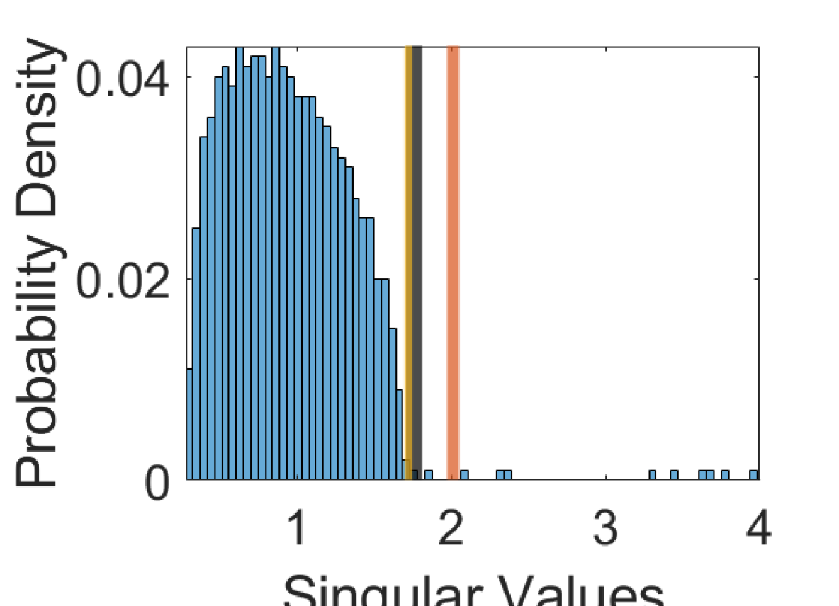
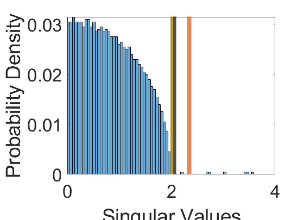
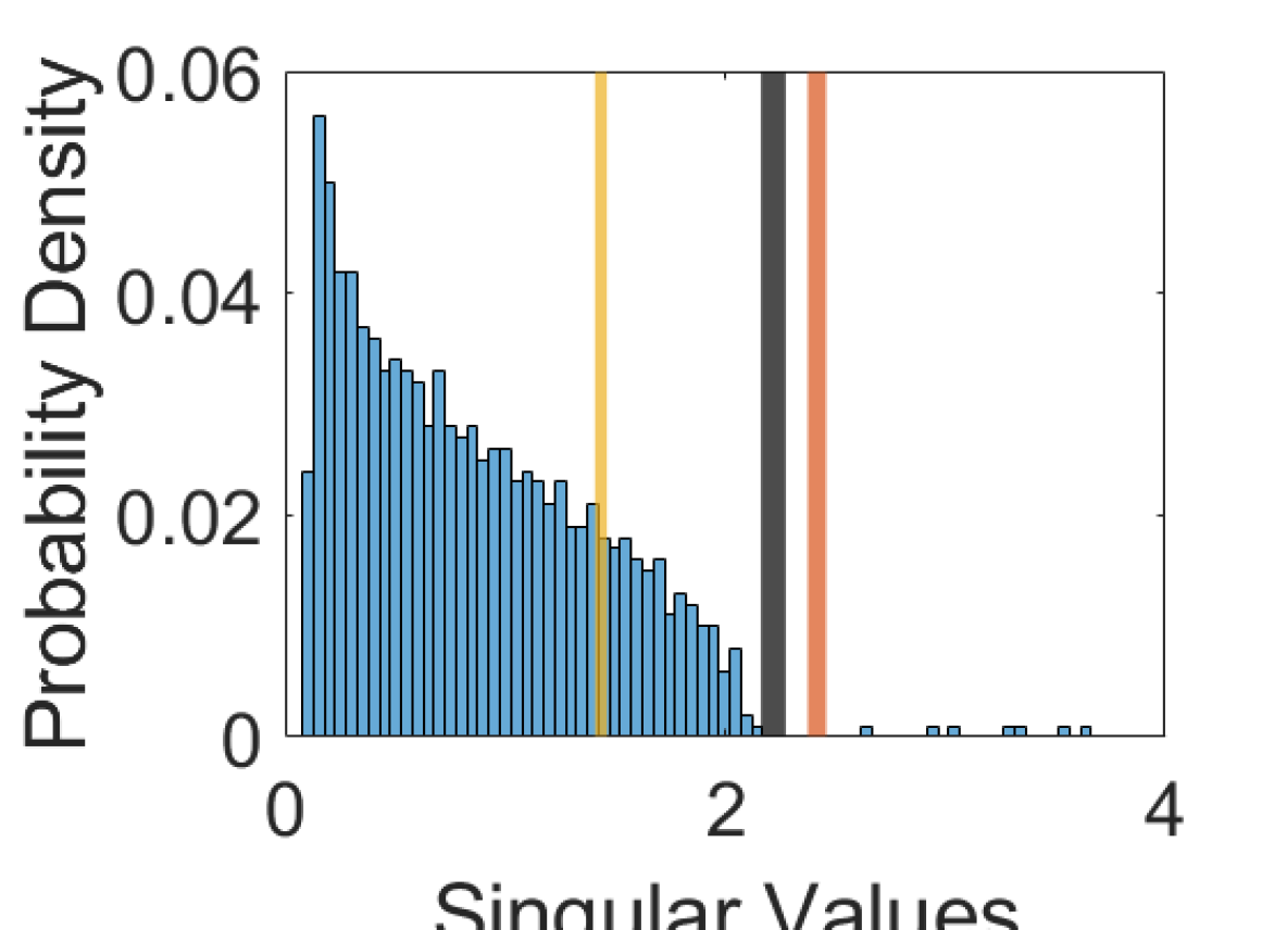
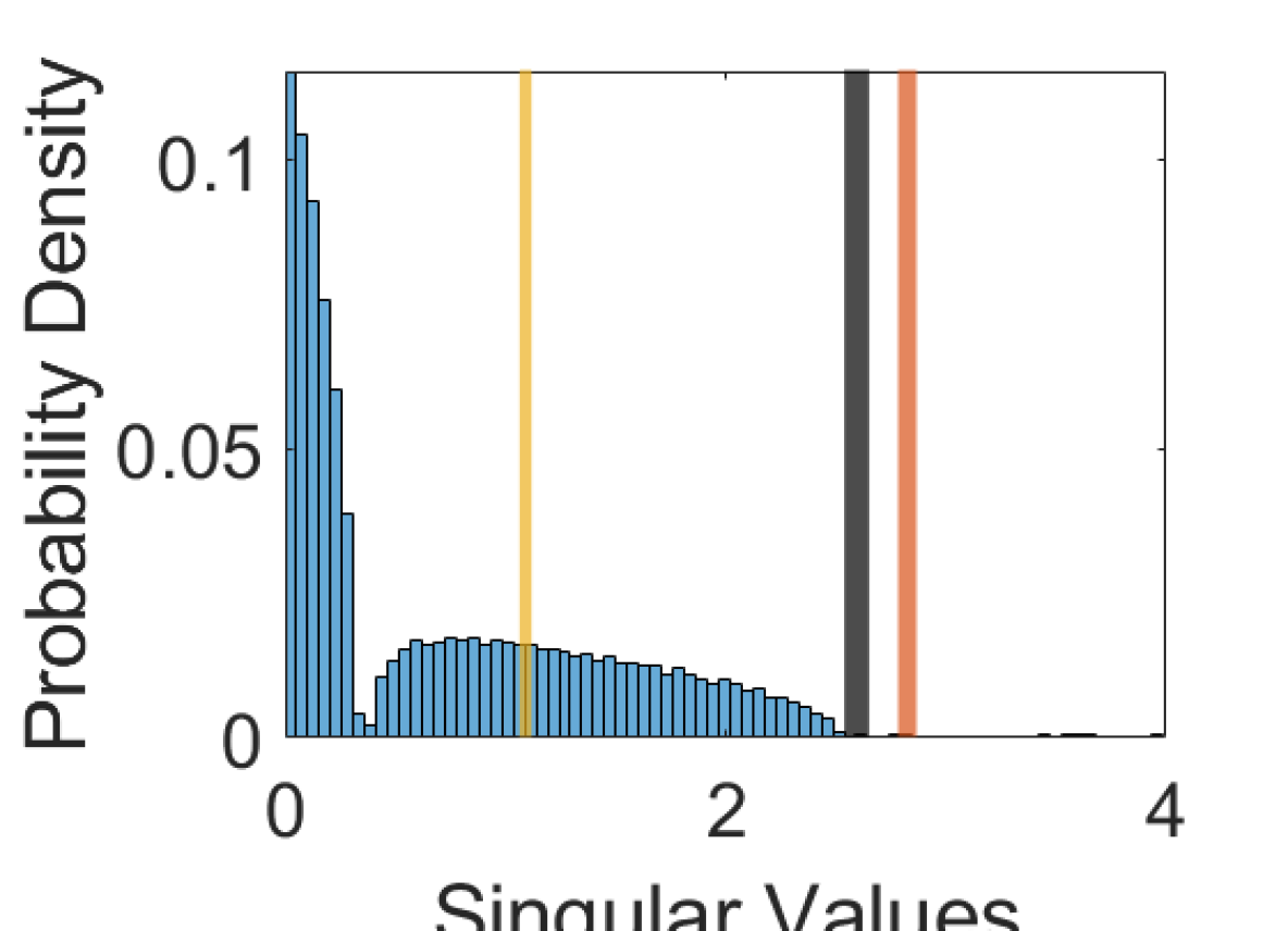
Figure 2. ESD of $\widetilde{S}$ when $n=2000$. The black and yellow lines are the estimated bulk edge from (41) and TRAD respectively. The red line is $\vartheta$ in (4) by ScreeNOT. From left to right: TYPE1 noise with $p/n=0.5$ and $p/n=1$ and TYPE2 noise with $p/n=0.5$ and $p/n=1$.

5.1.2. Rank estimation

To evaluate the rank estimation, the ground truth is determined with $\widehat{\alpha}$; that is $r^{+}$ is determined by $r^{+}_{*}:=\#\{i|d_{i}-\widehat{\alpha}>n^{-2/5}\}$, where $n^{-2/5}$ comes from the fact that the entries of $X$ are of 10 degrees of freedom. Note that since $\widehat{\alpha}$ is sufficiently close to $\alpha$, we can safely assume that $r^{+}=r^{+}_{*}$ and check the performance of our rank estimator $\widehat{r}^{+}$. In Figure 3, we compare the estimated rank using (42), the ScreeNOT rank, and the rank estimated by TRAD, which is the number of eigenvalues of $\widetilde{S}\widetilde{S}^{\top}$ larger than $\check{\sigma}(\widetilde{S})(1+\sqrt{p/n})$. TRAD always overestimates the rank for TYPE2 noise and sometimes overestimates the rank for TYPE1 noise. ScreeNOT rank is often underestimating the rank, with a larger error compared to our approach, and it does not seem to improve when $n$ grows. Our approach outperforms others. Note that since there is no gap of order $n^{-1/3}$ as in (42) to rule out eigenvalues of $\widetilde{S}\widetilde{S}^{\top}$ that do not contain information, when $n$ is small, like $300$, our rank estimator sometimes underestimates the rank.

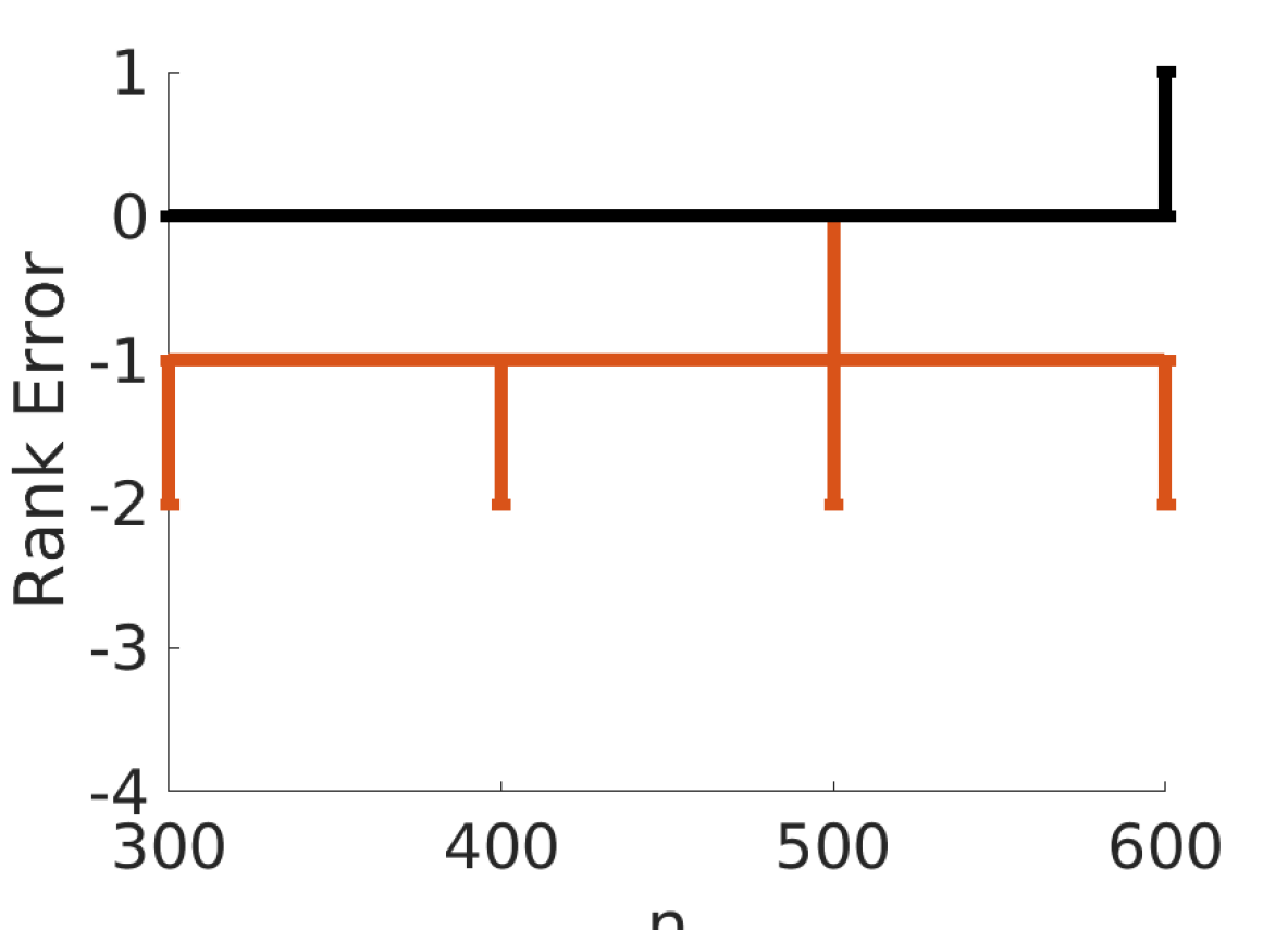
Figure 3. A comparison of different rank estimators, where we show $\widehat{r}^{+}-r^{+}$. The black (red and yellow respectively) lines are errors of rank estimator from our estimator (42) (ScreeNot and TRAD respectively). From left to right: TYPE1 noise with $p/n=0.5$ and $p/n=1$ and TYPE2 noise with $p/n=0.5$ and $p/n=1$. The solid and dashed magnets lines overlap for TYPE2 noise. Note that for Type 2 noise, the TRAD always overestimates $\widehat{r}^{+}$, and thus the error yellow lines are outside of the current scale.

5.1.3. Frobenius norm loss

In Figure 4, we show the Frobenius norm loss. When TYPE1 noise is considered, the loss of ScreeNOT is higher compared with other methods, TRAD has the lowest norm with statistical significance, and the loss of eOptShrink is similar to that of TRAD. When TYPE2 noise is considered, overall eOptShrink outperforms others with statistical significance.

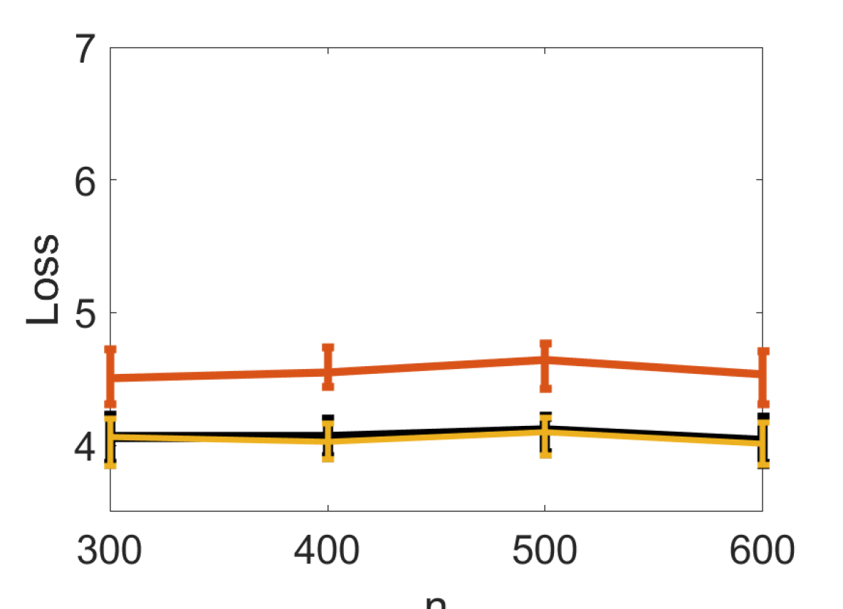
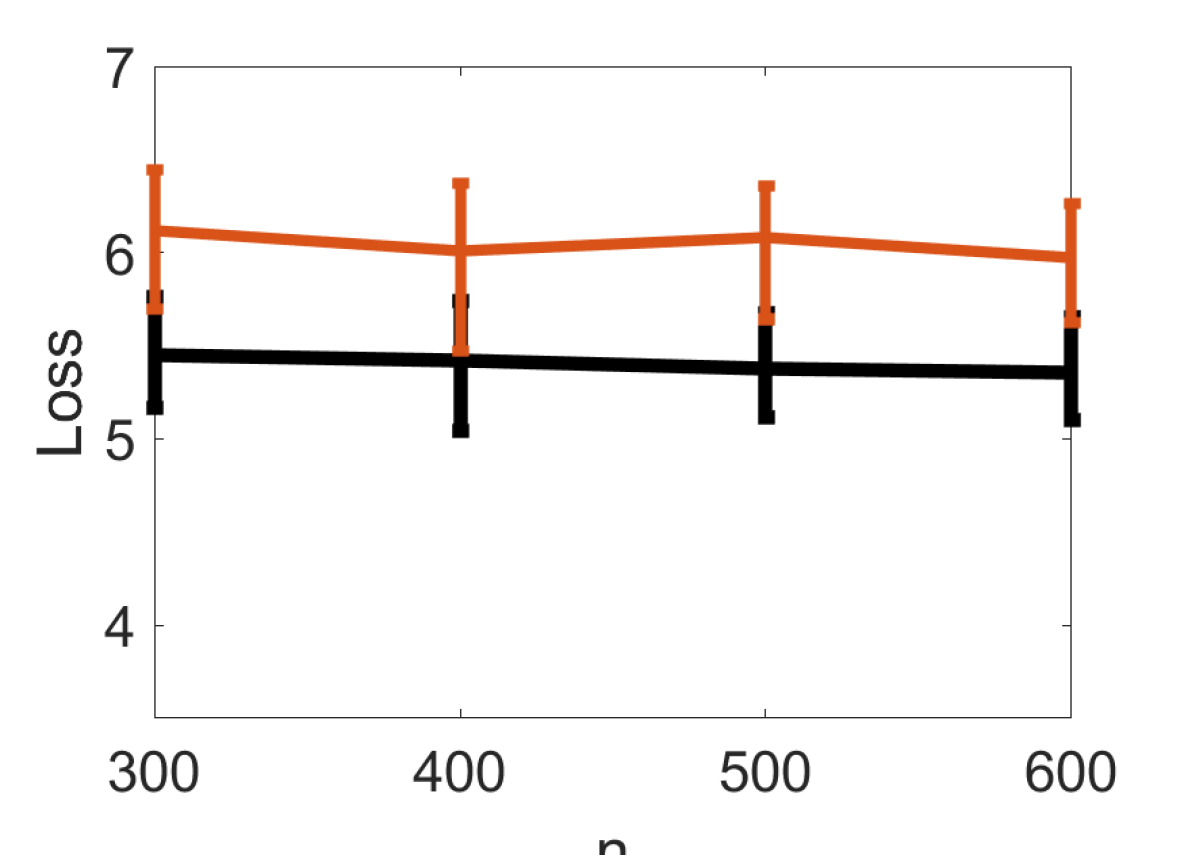
Figure 4. The Frobenius norm error of different algorithms. The black, red, and yellow lines are for eOptShrink, ScreeNOT, and TRAD respectively. From left to right: TYPE1 noise with $p/n=0.5$ and $p/n=1$ and TYPE2 noise with $p/n=0.5$ and $p/n=1$. In the TYPE2 noise, the yellow lines are not shown since they are too large.

Results in Sections 5.1.2 and 5.1.3 show that when TYPE1 noise is considered, TRAD always has the best performance. This is because TRAD has the closed form of $\lambda_{+}$ and optimal shrinkers. However, when the noise is TYPE2, the closed form is invalid and TRAD leads to a large error. ScreeNOT cannot detect weak signals and does not perform shrinkage, thus it always has high errors for both types of noise. eOptShrink has a similar performance as TRAD when $n$ is large under TYPE1 noise and has the best performance under TYPE2 noise. In summary, these simulations guarantee that (42) is a precise estimator of $r^{+}$. This finding supports the application of $\widehat{r}^{+}$ (42) in the proposed eOptShrink.

5.1.4. Optimal shrinkage estimation via $\widehat{F}_{\texttt{T}}(x)$, $\widehat{F}_{\texttt{imp}}(x)$ and $\widehat{F}_{\texttt{e}}(x)$

We compare how well we could use the proposed pseudo-distribution $\widehat{F}_{\texttt{e}}$ and existing $\widehat{F}_{\texttt{T}}(x)$ and $\widehat{F}_{\texttt{imp}}(x)$ to estimate the optimal shrinkage in Proposition 2.6 via estimating $d_{r^{+}}$ and $\sqrt{a_{1,r^{+}}a_{2,r^{+}}}$. Set $k=2r$ for $\widehat{F}_{\texttt{imp}}(x)$ in (40) by using the oracle rank information. For a fair comparison, we set $c$ so that $\lfloor n^{c}\rfloor=2r$ when we modify the top $2\widehat{r}^{+}$ eigenvalues of $\widetilde{S}\widetilde{S}^{\top}$ in $\widehat{F}_{\texttt{e}}(x)$ (47). As shown in the last simulation, our rank estimator is precise when $n$ is large, but errors happen when $n$ is small. Since $\widehat{F}_{\texttt{T}}(x)$ and $\widehat{F}_{\texttt{e}}(x)$ depend on the estimated rank $\widehat{r}^{+}$, we consider the case when $\widehat{r}^{+}$ satisfies $\widehat{r}^{+}-r^{+}=-2,\ldots,+2$; that is, we study how badly the erroneous rank estimate could impact the final result. In Figures 5 and 6, the error ratio of estimating $d_{\min\{r^{+},\widehat{r}^{+}\}}$ and $\sqrt{a_{1,\min\{r^{+},\widehat{r}^{+}\}}a_{2,\min\{r^{+},\widehat{r}^{+}\}}}$ respectively for $n=300$ and $n=600$ with different pseudo-distributions. Note that the $r^{+}$th singular value is the smallest “strong” one, which is the most challenging one to recover. For each $n$, we repeat the simulation for $100$ times. Clearly, our approach has the lowest error ratio with a statistical significance, and the error decreases when $n$ grows from $300$ to $600$. This result shows that compared with ScreeNot, eOptShrink is robust to a slightly erroneous rank estimation. We thus have a theoretical guarantee for the application of $\widehat{F}_{\texttt{e}}(x)$ in eOptShrink.

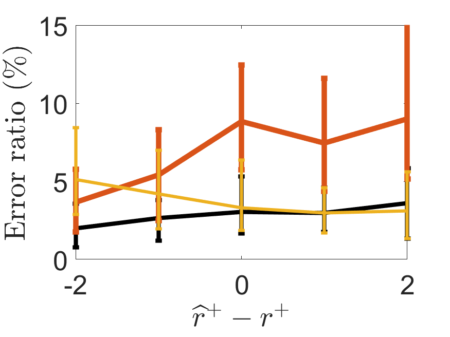
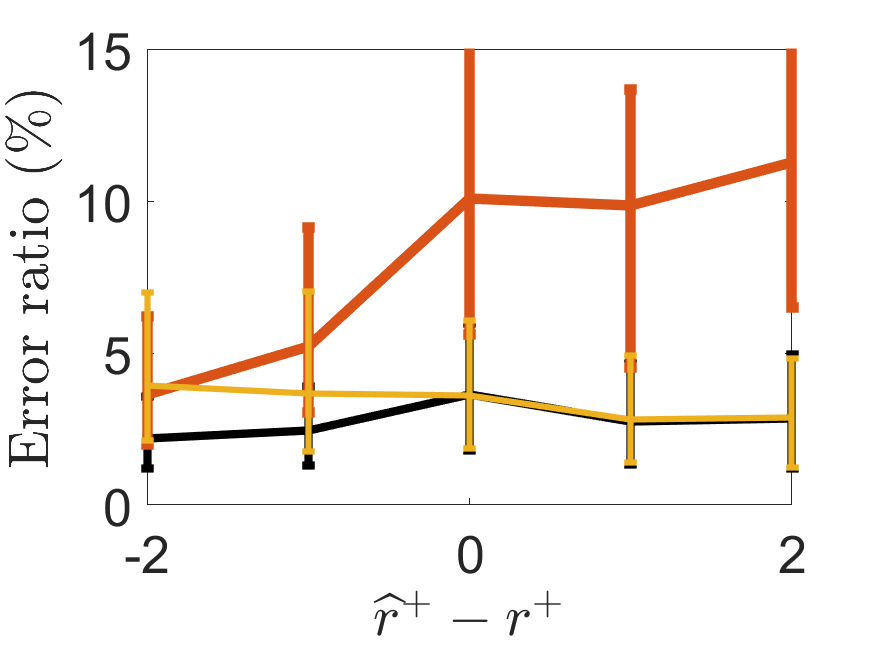
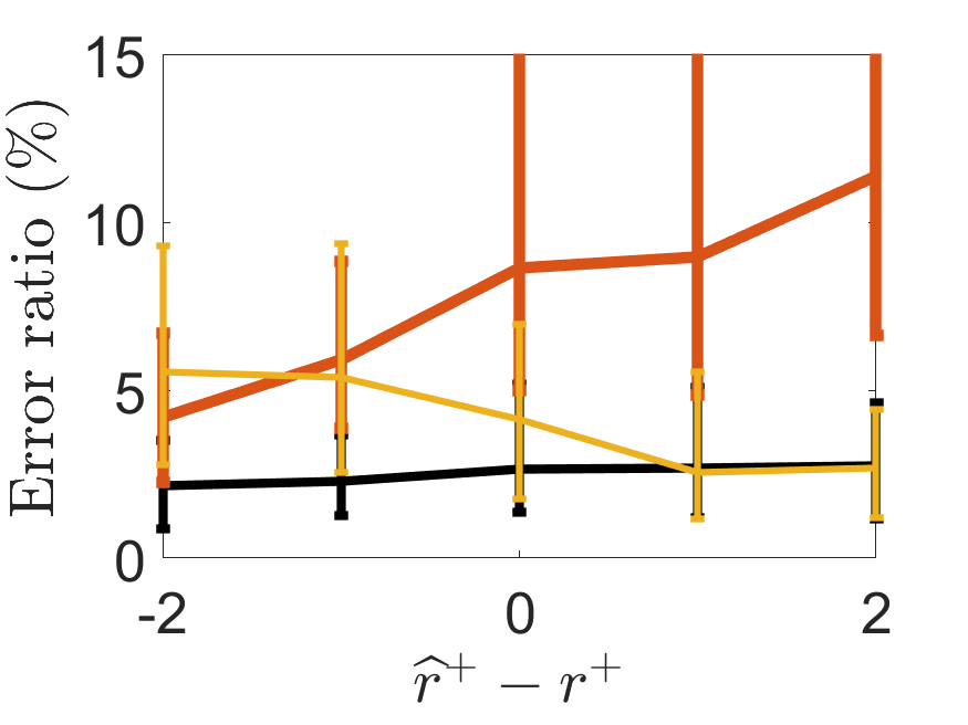
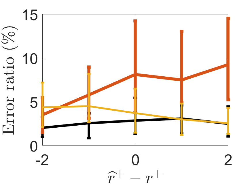
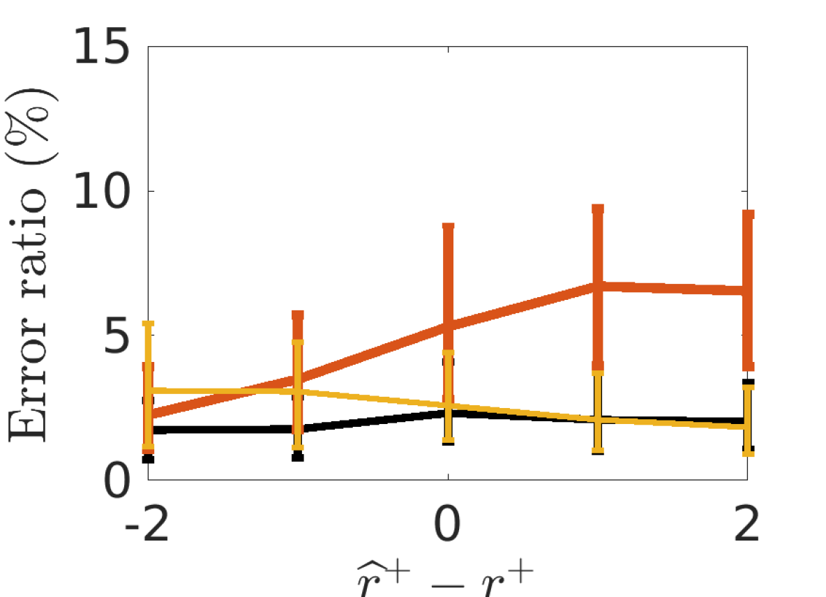
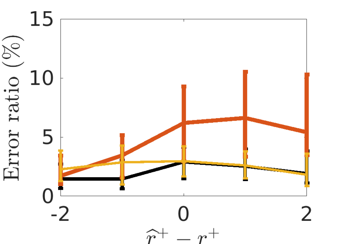
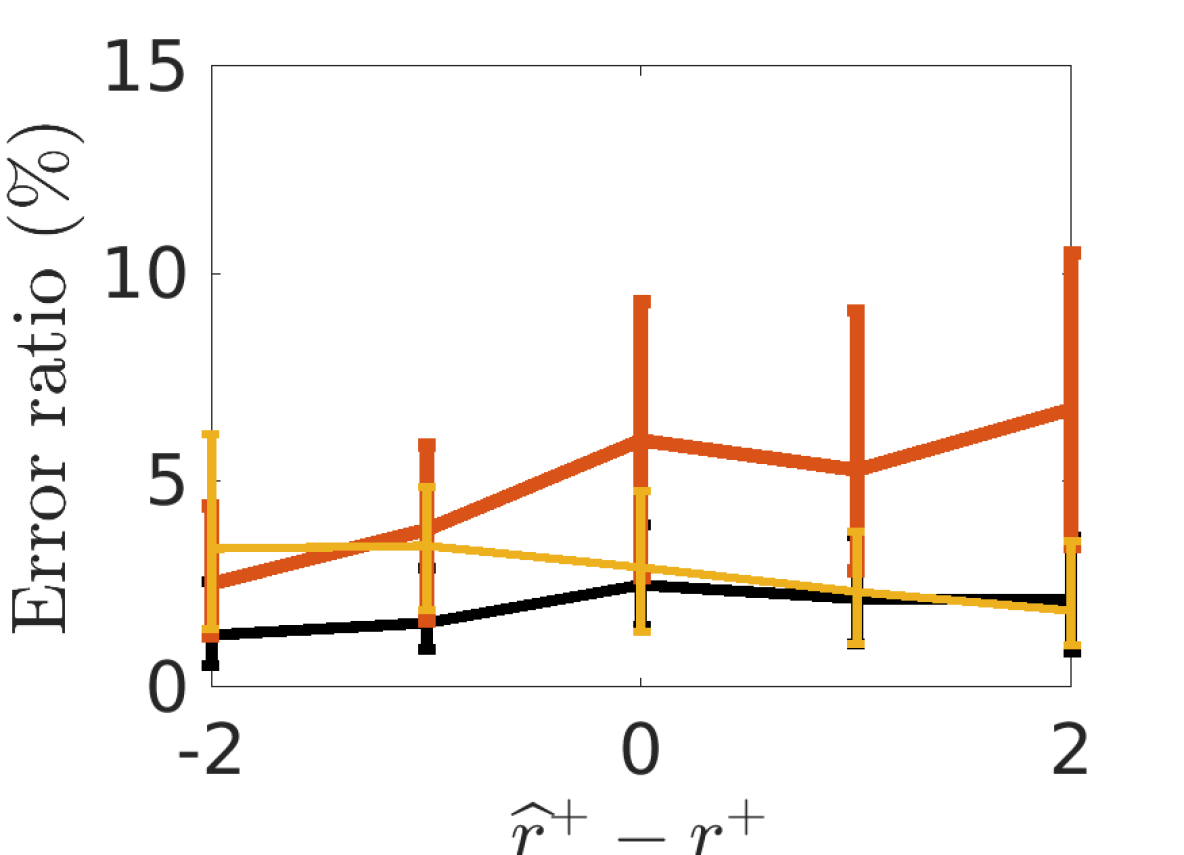
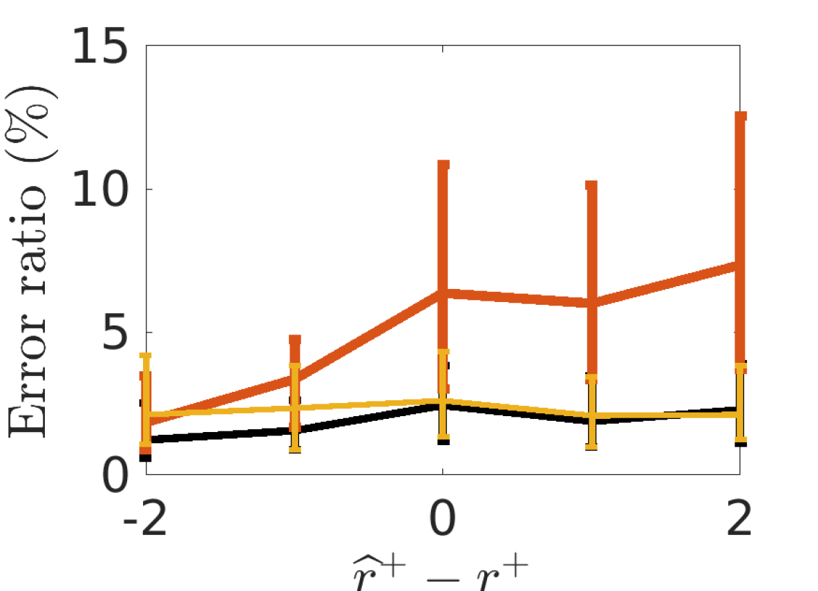
Figure 5. Interquartile errorbars of error ratios of estimating $d_{\min\{r^{+},\widehat{r}^{+}\}}$ by using $F_{\texttt{e}}(x)$, $F_{\texttt{T}}(x)$ and $F_{\texttt{imp}}(x)$, shown in black, yellow, and red lines respectively. If the corresponding error ratio is too high, the associated curve is not totally plotted to enhance the visualization. From left to right: TYPE1 noise with $p/n=0.5$ and $p/n=1$ and TYPE2 noise with $p/n=0.5$ and $p/n=1$. $n=300$ is shown in the first row and $n=600$ in the second row.

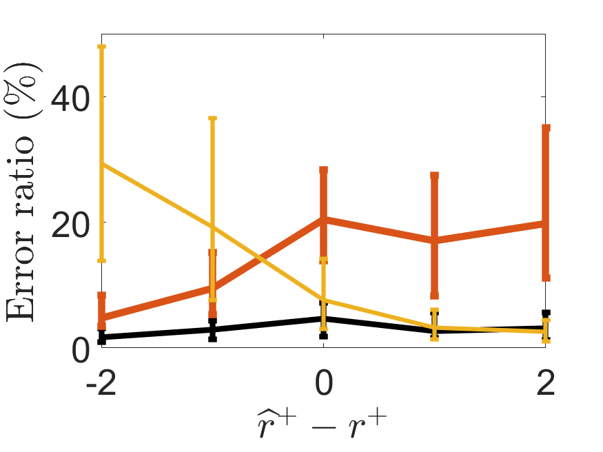
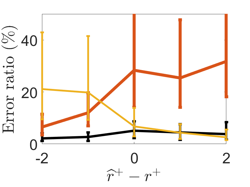
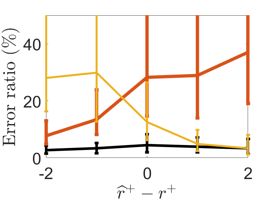
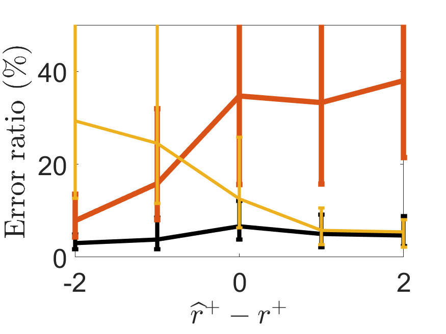
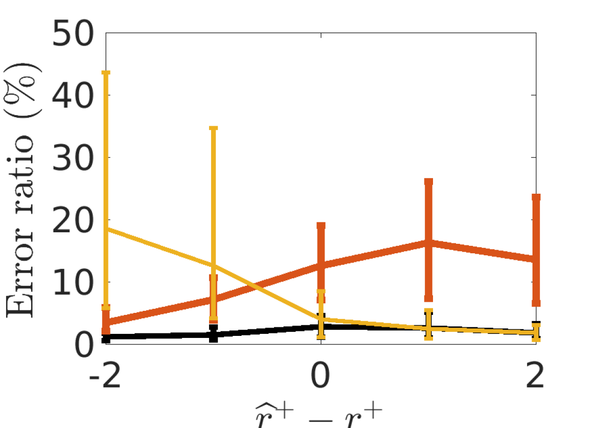
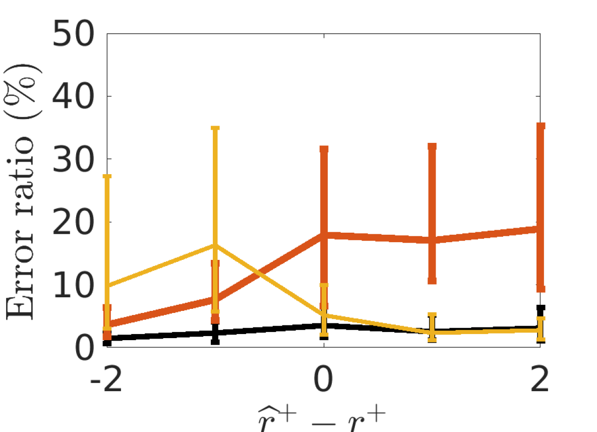
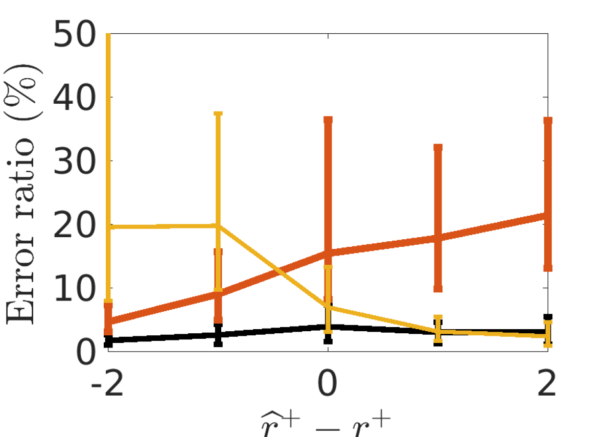
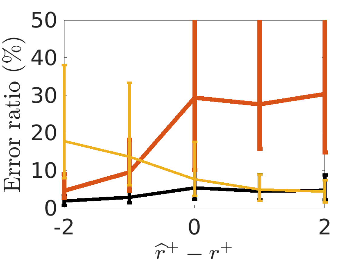
Figure 6. Interquartile errorbars of error ratios of estimating $\sqrt{a_{1,\min\{r^{+},\widehat{r}^{+}\}}a_{2,\min\{r^{+},\widehat{r}^{+}\}}}$ using $F_{\texttt{e}}(x)$, $F_{\texttt{T}}(x)$ and $F_{\texttt{imp}}(x)$, shown in black, yellow, and red lines respectively. If the corresponding error ratio is too high, the associated curve is not totally plotted to enhance the visualization. From left to right: TYPE1 noise with $p/n=0.5$ and $p/n=1$ and TYPE2 noise with $p/n=0.5$ and $p/n=1$. $n=300$ is shown in the first row and $n=600$ in the second row.

5.2. Fetal ECG extraction problem

In our previous work [50], TRAD is the critical step of the algorithm to recover the mECG when we have only one or two ta-mECG channels. The algorithm is composed of two steps. The first step is mainly for two channels, and we ignore it when we only have one channel. The second step is composed of two substeps. Step 2-1 is designed to detect the maternal R peaks from the single channel ta-mECG, which is not the concern of OS. Step 2-2 is mainly illustrated in Figure 1, where we view fECG as noise and mECG as the signal, and OS is applied to recover mECG from the ta-mECG. As is mentioned in Introduction, fECG, when viewed as noise, is not white, and there is a dependence among segments. Thus, it is natural to consider replacing TRAD in [50] by ScreeNOT or eOptShrink. We consider a semi-real simulated database and a real-world database from 2013 PhysioNet/Computing in Cardiology Challenge [48], abbreviated as CinC2013.

5.2.1. Semi-real simulated database

The semi-real ta-mECG data is constructed from the Physikalisch-Technische Bundesanstalt (PTB) Database https://physionet.org/physiobank/database/ptbdb/, abbreviated as PTBDB following the same way detailed in [50]. The database contains 549 recordings from 290 subjects (one to five recordings for one subject) aged 17 to 87 with the mean age 57.2. 52 out of 290 subjects are healthy. Each recording includes simultaneously recorded conventional 12 lead and the Frank lead ECGs. Each signal is digitalized with the sampling rate 1000 Hz. More technical details can be found online. Take 57-second Frank lead ECGs from a healthy recording, denoted as $V_{x}(t)$, $V_{y}(t)$ and $V_{z}(t)$ at time $t\in\mathbb{R}$, as the maternal vectocardiogram (VCG). Take $(\theta_{xy},\theta_{z})=(\frac{\pi}{4},\frac{\pi}{4})$, and the simulated mECG is created by $\text{mECG}(t)=(V_{x}(t)\cos{\theta_{xy}}+V_{y}(t)\sin{\theta_{xy}})\cos{\theta_{z}}+V_{z}(t)\sin{\theta_{z}}$. We create 40 mECGs. The simulated fECG of healthy fetus are created from another 40 recordings from healthy subjects, where $114$-second V2 and V4 recordings are taken. The simulated and simulated fECG come from different subjects. The simulated fECG then are resampled at $500$ Hz. As a result, the simulated fECG has about double the heart rate compared with the simulated mECG if we consider both signals sampled at $1000$ Hz. The amplitude of the simulated fECG is normalized to the same level of simulated mECG and then multiplied by $0<R<1$ shown in the second column of Table 1 to make the amplitude relationship consistent with the usual situation of real ta-mECG signals. We generate 40 simulated healthy fECGs. The clean simulated ta-mECG is generated by directly summing simulated mECG and fECG. We then create a simulated noise starting with a random vector $\textbf{x}=(x_{1},x_{2},x_{3},\ldots)$ with i.i.d entries with student t-10 distribution. The noise is then created and denotes as z with the entries $z_{i}=(1+0.5\sin((i\mod 500)/500))(x_{i}+x_{i+1}+x_{i+2})$. The final simulated ta-mECG is generated by adding the created noise to the clean simulated ta-mECG according to the desired SNR ratio shown in the first column of Table 1. As a result, we acquire $40$ recordings of $57$ seconds simulated ta-mECG signals with the sampling rate $1000$ Hz.

For each recording in the simulated database, we apply different OS algorithms, including TRAD, ScreeNot and eOptShrink, in Step 2-2 and report the root mean square error (RMSE) of the recovered mECG by comparing the recovered mECG with the ground truth mECG. See Table 1 for the result. As is shown in Table 1, eOptShrink has the smallest RMSE in all scenarios compared with ScreeNot and TRAD. A lower SNR results in a higher RMSE over every amplitude ratio $R$ for all OS methods. Moreover, a higher fECG amplitude results in a higher noise level for the recovery of mECG and thus a higher RMSE over all SNRs for all OS methods.

SNR	$R$	TRAD	ScreeNot	eOptShrink
$1$ dB	1/4	12.20 $\pm$ 1.57	9.25* $\pm$ 1.91	8.86*$\star$ $\pm$ 1.76
	1/6	10.03$\pm$ 1.31	7.76*$\pm$ 1.60	7.45*$\star\pm$ 1.47
	1/8	8.73 $\pm$ 1.11	6.81* $\pm$ 1.34	6.57* $\star\pm$ 1.24
$0$ dB	1/4	12.56 $\pm$ 1.69	9.29* $\pm$ 2.07	8.97* $\star\pm$ 1.83
	1/6	10.31 $\pm$ 1.36	7.74*$\pm$ 1.61	7.48* $\star\pm$ 1.44
	1/8	8.98 $\pm$ 1.18	6.88* $\pm$ 1.40	6.62* $\star\pm$ 1.28
$-1$ dB	1/4	12.94 $\pm$ 1.76	9.31* $\pm$2.09	9.07*$\star\pm$ 1.79
	1/6	10.66 $\pm$1.47	7.88*$\pm$ 1.62	7.61*$\star\pm$ 1.46
	1/8	9.27$\pm$ 1.26	6.94* $\pm$ 1.42	6.71* $\star\pm$ 1.26

Table 1. The comparison of RMSE for the mECG morphology of different algorithms applied to the simulated ta-mECG database. $R$ is the simulated fECG amplitude. All results are presented as mean $\pm$ standard deviation. The asteroids next to mean stand for the statistical significance when comparing ScreeNot or eOptShrink and TRAD using the paired t-test, and the stars next to mean stand for the statistical significance when comparing ScreeNot and eOptShrink.

5.2.2. CinC2013 database

Each recording in CinC2013 includes four ta-mECG channels and the simultaneously recorded directly contact fECG, all resampled at the sampling rate 1000 Hz and last for 1 minute. For each channel of each recording, we run the fECG extraction algorithm with different OS algorithms in Step 2-2. In Figure 7, we compared the recovered mECG and the detected fetal R peak locations by TRAD, ScreeNot, and eOptShrink. It is obvious that eOptShrink has a better recovery of the morphology of mECG and hence the fECG. Particularly, we can easily visualize the ventricular activity residues indicated by purple arrows when the mECG is recovered by ScreeNot, but these residues are removed by eOptShrink. As a result, with eOptShrink, the electrophysiological properties of both the maternal and fetal hearts could be better evaluated. The clinical application will be reported in our future work.

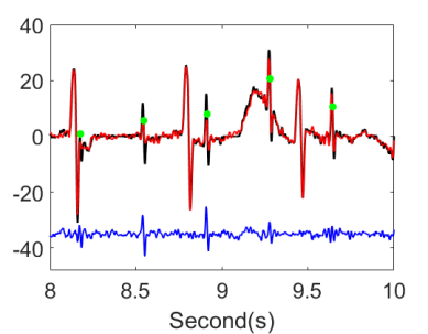
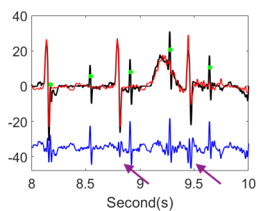
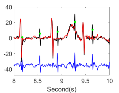
Figure 7. A comparison of mECG and fECG recovery by different algorithms (recording 1 and channel 1 from CinC2013). The left panel is by TRAD, the middle one is by ScreeNot, and the right one is by eOptShrink. The original ta-mECG is shown in black with the recovered mECG superimposed in red and the fetal R peaks labeled by experts are superimposed as green dots. The difference of the ta-mECG and the recovered mECG is shown in blue, which represents the recovered fetal ECG. The purple arrows indicate the ventricular activity residue, which is the limitation of the hard threshold approach like ScreeNot.

Table S.1. List of default notations, part 1.

$S$	clean data matrix of size $p\times n$
$\beta_{n}$,$\beta$	$\beta_{n}:=p/n\to\beta$ as $p,\ n\to\infty$
$r$	rank of $S$
$\{d_{i}\}_{i=1}^{r}$	singular values of $S$
$\{\mathbf{u}_{i},\ \mathbf{v}_{i}\}_{i=1}^{r}$	left and right singular vectors of $S$
$Z$	$Z=A^{1/2}XB^{1/2}$, noise matrix of size $p\times n$
$X$	noise matrix with i.i.d. entries
$A$,$B$	colorness and dependence for noise
$\{\sigma_{i}^{a}\}_{i=1}^{p}$	eigenvalues of $A$
$\{\sigma_{i}^{b}\}_{i=1}^{n}$	eigenvalues of $B$
$\{\lambda_{i}\}_{i=1}^{p}$	eigenvalues of $ZZ^{\top}$
$\widetilde{S}$	$\widetilde{S}=S+Z$, noisy data matrix
$\{\widetilde{\lambda}_{i}\}_{i=1}^{p}$	eigenvalues of $\widetilde{S}\widetilde{S}^{\top}$
$\{\widetilde{\bm{\xi}}_{i}\}_{i=1}^{p}$	left singular vectors of $\widetilde{S}$
$\{\widetilde{\bm{\zeta}}_{i}\}_{i=1}^{n}$	right singular vectors of $\widetilde{S}$
$G_{\mathbf{u}}^{n}$, $G_{\mathbf{v}}^{n}$	independent matrices for generating $\mathbf{u}_{i}$ and $\mathbf{v}_{i}$
$\nu$	probability measure of entires in $G_{\mathbf{u}}^{n}$ and $G_{\mathbf{v}}^{n}$
$\varphi$, $\varphi^{*}$	the shrinker and optimal shrinkger
$\widehat{\varphi}_{i}$	estimator of $\varphi_{i}=\varphi^{*}(\widetilde{\lambda}_{i})$
$\widehat{S}_{\varphi}$	Estimator constructed by shrinker $\varphi$.
$\vartheta$	The hard threshold
$\pi^{(n)}_{H}$	empirical spectral distribution (ESD) of an $n\times n$ symmetric matrix $H$
$m_{\nu}(z)$	Steiljes transform for probability measure $\nu$ for $z\in\mathbb{C}^{+}$
$\mathcal{G}_{1},\ \mathcal{G}_{2}$	Green functions for $ZZ^{\top}$ and $Z^{\top}Z$
$m_{1},\ m_{2}$	Stieltjes transforms of ESD of $ZZ^{\top}$ and $Z^{\top}Z$
$\widetilde{\mathcal{G}}_{1},\ \widetilde{\mathcal{G}}_{2}$	Green functions for $\widetilde{S}\widetilde{S}^{\top}$ and $\widetilde{S}^{\top}\widetilde{S}$
$\widetilde{m}_{1},\ \widetilde{m}_{2}$	Stieltjes transforms of ESD of $\widetilde{S}\widetilde{S}^{\top}$ and $\widetilde{S}^{\top}\widetilde{S}$
$\mathsf{m}^{(p)}_{1c}(z)$	$\beta_{n}\int\frac{x}{-z\left[1+x\mathsf{m}^{(n)}_{2c}(z)\right]}\pi_{A}^{(p)}(dx)$
$\mathsf{m}^{(n)}_{2c}(z)$	$\int\frac{x}{-z\left[1+x\mathsf{m}^{(p)}_{1c}(z)\right]}\pi_{B}^{(n)}(dx)$
$\varrho^{(p)}_{1c}$, $\varrho^{(p)}_{2c}$	Corresponding densities derived from $\mathsf{m}^{(p)}_{1c}(z)$ and $\mathsf{m}^{(n)}_{2c}(z)$
$m^{(p)}_{1c}(z)$	$\int\frac{1}{-z\left[1+x\mathsf{m}^{(n)}_{2c}(z)\right]}\pi_{A}^{(p)}(dx)$
$m^{(n)}_{2c}(z)$	$\int\frac{1}{-z\left[1+x\mathsf{m}^{(p)}_{1c}(z)\right]}\pi_{B}^{(n)}(dx)$

Table S.2. List of default notations, part 2.

$\rho_{1c}^{(p)},\ \rho_{2c}^{(n)}$	Corresponding densities derived from $m^{(p)}_{1c}(z)$ and $m^{(n)}_{2c}(z)$
$\lambda_{+}$	the right most edge of support of $\varrho_{1c}$, $\varrho_{2c}$, $\rho_{1c}$, and $\rho_{2c}$ on $(0,\infty)$
$\Delta(d_{i})$	$(d_{i}-\alpha)^{1/2}$
$\mathcal{T}(z)$	$\mathcal{T}(z)=zm_{1c}(z)m_{2c}(z)$, the D-transform of $\rho_{1c}$
$\alpha$	threshold $\alpha=1/\sqrt{\mathcal{T}(\lambda_{+})}$
$\phi_{n}$	bound for entries of $X$
$r^{+}$	the index of singular values that are sufficiently strong to pass the BBP phase transition
$\mathbb{O}_{+}$	the set $\{1,\cdots,r^{+}\}$
${\mathcal{P}}_{\bf A},\ {\mathcal{P}}^{\prime}_{\bf A}$	the random projections for $\textbf{A}\subset\mathbb{O}^{+}$, ${\mathcal{P}}_{\bf A}:=\sum_{k\in\bf A}\widetilde{\xi}_{k}\widetilde{\xi}_{k}^{\top}$ and ${\mathcal{P}}^{\prime}_{\bf A}:=\sum_{k\in\bf A}\widetilde{\zeta}_{k}\widetilde{\zeta}_{k}^{\top}$
$\nu_{i}(\textbf{A})$	defined as $\begin{cases}\min_{j\notin\textbf{A}}|d_{j}-d_{i}|,&\textup{ if }i\in\textbf{A},\\ \min_{j\in\textbf{A}}|d_{j}-d_{i}|,&\textup{ if }i\notin\textbf{A}\end{cases}$
$\widehat{\lambda}_{j}$	defined as $\widetilde{\lambda}_{k+1,n}+\frac{1-\left(\frac{j-1}{k}\right)^{2/3}}{2^{2/3}-1}\left(\widetilde{\lambda}_{2k+1,n}-\widetilde{\lambda}_{k+1,n}\right)$
$F_{imp}$	The cumulative eigenvalue distribution function (CDF) constructed by imputation method
$F_{1}$	The CDF of $ZZ^{\top}$
$\widehat{m}_{1,i}$, $\widehat{m}_{2,i}$	Estimators of $m_{1c}(\widetilde{\lambda}_{i})$ and $m_{2c}(\widetilde{\lambda}_{i})$
$\widehat{m}_{1,i}^{\prime}$, $\widehat{m}_{2,i}^{\prime}$	Estimators of $m_{1c}^{\prime}(\widetilde{\lambda}_{i})$ and $m_{2c}^{\prime}(\widetilde{\lambda}_{i})$
$\theta(x):=\mathcal{T}^{-1}(x^{-2}),\ a_{1}(x):=\frac{m_{1c}(\theta(x))}{x^{2}\mathcal{T}^{\prime}(\theta(x))},\ a_{2}(x):=\frac{m_{2c}(\theta(x))}{x^{2}\mathcal{T}^{\prime}(\theta(x))}$
$\widehat{\mathcal{T}}_{i}=\widetilde{\lambda}_{i}\widehat{m}_{1,i}\widehat{m}_{2,i},\quad\widehat{\mathcal{T}}^{\prime}_{i}=\widehat{m}_{1,i}\widehat{m}_{2,i}+\widetilde{\lambda}_{i}\widehat{m}^{\prime}_{1,i}\widehat{m}_{2,i}+\widetilde{\lambda}_{i}\widehat{m}^{\prime}_{2,i}\widehat{m}_{1,i}$
$\widehat{d}_{i}=\sqrt{\frac{1}{\widehat{\mathcal{T}}_{i}}},\quad\widehat{a}_{1,i}=\frac{\widehat{m}_{1,i}}{\widehat{d}_{i}^{2}\widehat{\mathcal{T}}^{\prime}_{i}}\ \mbox{ and }\ \widehat{a}_{2,i}=\frac{\widehat{m}_{2,i}}{\widehat{d}_{i}^{2}\widehat{\mathcal{T}}^{\prime}_{i}}$
$\gamma_{j}:=\sup_{x}\{\int_{x}^{+\infty}\rho_{1c}(x)dx>\frac{j-1}{n}\}$
$\varkappa_{i}:=i^{2/3}n^{-2/3},$ for $i=1,\ldots,n$
$\eta_{i}:=n^{-3/4}+n^{-5/6}i^{1/3}+n^{-1/2}\phi_{n}$
$\eta_{\ell}(E)\mbox{ satisfies }n^{1/2}\left[\Psi^{2}(E+i\eta_{l}(E))+\frac{\phi_{n}}{n\eta_{l}(E)}\right]=1$
$\kappa_{z}:=|E-\lambda_{+}|$, for $z=E+i\eta\in\mathbb{C}$
$\Psi(z):=\sqrt{\frac{\text{Im }\mathsf{m}_{2c}(z)}{n\eta}}+\frac{1}{n\eta}$
$\omega(d_{i}):=\phi_{n}\Delta^{2}(d_{i})+n^{-1/2}\Delta(d_{i})$
$\psi_{1}(d_{i}):=\phi_{n}+\frac{n^{-1/2}}{\Delta(d_{i})}$
$I_{i}:=[\theta(d_{i})-n^{\epsilon}\omega(d_{i}),\theta(d_{i})+n^{\epsilon}\omega(d_{i})]$
$I_{0}:=[0,\lambda_{+}+n^{3\epsilon}\phi_{n}^{2}+n^{-2/3+3\epsilon}]$
$I:=I_{0}\cup\bigcup_{i\in\mathbb{O}_{\epsilon}}I_{i}$
$\Omega_{i}:=\Big{\{}x\in[\lambda_{i-r-1},\lambda_{+}+c_{0}n^{2\epsilon}(\phi_{n}^{2}+n^{-2/3})]:$
$\qquad\text{dist}\Big{(}x,\text{Spec}({ZZ^{\top}})\Big{)}>n^{-1+\epsilon}\alpha_{+}^{-1}+n^{\epsilon}\eta_{l}(x)\Big{\}}$
$\mathbf{D}_{1}(\tau_{1},\varsigma):=\{z=E+i\eta:\lambda_{+}<E<\varsigma,\,-\tau_{1}<\eta<\tau_{1}\}$
$\mathbf{D}_{2}(\tau_{2},\varsigma):=\{\zeta=E+i\eta:\alpha<E<1/\sqrt{\mathcal{T}(\varsigma)},\,-\tau_{2}<\eta<\tau_{2}\}$
$S_{0}(\varsigma_{1},\varsigma_{2},\omega):=S(\varsigma_{1},\varsigma_{2})\cap\{z=E+i\eta:\eta\geq n^{-1+\omega}\}$
$S(\varsigma_{1},\varsigma_{2}):=\{z=E+i\eta:\lambda_{+}-\varsigma_{1}\leq E\leq\varsigma_{2}\lambda_{+},0<\eta\leq 1\}$
$\widetilde{S}_{0}(\varsigma_{1},\varsigma_{2},\omega):=S_{0}(\varsigma_{1},\varsigma_{2},\omega)\cap\left\{z=E+i\eta:n^{1/2}\left(\Psi^{2}(z)+\frac{\phi_{n}}{n\eta}\right)\leq n^{-\omega/2}\right\}$
$S_{out}(\varsigma_{2},\omega):=\{E+i\eta:\lambda_{+}+n^{\omega}(n^{-2/3}+n^{-1/3}\phi_{n}^{2})\leq E\leq\varsigma_{2}\lambda_{+},\eta\in[0,1]\}$
$H(z):=\begin{pmatrix}0&z^{1/2}Z\\ z^{1/2}Z^{\top}&0\end{pmatrix},\quad\widetilde{H}(z):=\begin{pmatrix}0&z^{1/2}\widetilde{S}\\ z^{1/2}\widetilde{S}^{\top}&0\end{pmatrix}$
$G(z):=(H-z)^{-1},\quad\widetilde{G}(z):=(\widetilde{H}-z)^{-1},\quad\mathbf{D}=\begin{pmatrix}0&z^{1/2}D\\ z^{1/2}D&0\end{pmatrix},\quad\mathbf{U}=\begin{pmatrix}U&0\\ 0&V\end{pmatrix}$
$\Pi(z):=\left({\begin{array}[]{*{20}c}{\Pi_{1}}(z)&0\\ 0&{\Pi_{2}}(z)\\ \end{array}}\right),\quad\Pi_{1}(z):=-z^{-1}\left(1+\mathsf{m}_{2c}(z)A\right)^{-1},\quad\Pi_{2}(z):=-z^{-1}(1+\mathsf{m}_{1c}(z)B)^{-1}.$
$\overline{\Pi}(z):=\begin{pmatrix}m_{1c}(z)I_{r}&0\\ 0&m_{2c}(z)I_{r}\end{pmatrix},\quad\Omega(z):=\mathbf{U}^{\top}G(z)\mathbf{U}-\overline{\Pi}(z)$

Appendix S.1 More results: simulated signal

Following the same approach in Section 5.1, in this section we provide a more extensive numerical study with more $D_{A}$ and $D_{B}$ using the distributions proposed in [19]. We create three types of one-sided noises so that $D_{B}$ is the identity matrix $I_{n}$ and $D_{A}$ follows the eigenvalue distribution of Mix2, Unif[1,10], or Fisher3n, where Mix2 stands for an equal mixture of $1$ and $10$ as eigenvalues, Unif[1,10] stands for sampling eigenvalues uniformly from [1, 10], and Fisher3n stands generating eigenvalues from the eigenvalues of $W^{\top}W$, where $W\in\mathbb{R}^{3p\times p}$ is a random matrix with i.i.d Gaussian entries with mean $0$ and variance $1/(3p)$. Moreover, by the same approach mentioned in Section 5.1, the resulting $\widehat{\alpha}$ for Mix2, Unif[1,10], or Fisher3n are $1.9160\pm 0.0211$, $1.2477\pm 0.0182$, and $1.2237\pm 0.0156$ respectively, where we show the mean $\pm$ standard deviation over 100 realizations with $n^{\prime}=10000$. We also generate three types of two-sided noises, where $D_{A}$ and $D_{B}$ follow Mix2 and Unif[1,10], Mix2 and Fisher3n, and Unif[1,10] and Fisher3n respectively, and the resulting $\widehat{\alpha}$ has mean $\pm$ standard deviation as $2.1354\pm 0.0206$, $2.0779\pm 0.0177$, and $1.4158\pm 0.0135$ respectively, where we show the mean $\pm$ standard deviation over 100 realizations with $n^{\prime}=10000$. The signal matrix is designed in the same way as that in Section 5.1.

As in Section 5.1.1, in Figure S.1, we compare the estimated rank using (42), the ScreeNOT rank, and the rank estimated by TRAD when $p/n=1$ with different $n$. Similar to the results of TYPE2 noise, TRAD always overestimates the rank for all combinations of noise types, and ScreeNOT rank often underestimates the rank with a larger error compared to eOptShrink.

In Figure S.2, we show the Frobenius norm loss as that studied in Section 5.1.3 when $p/n=1$ with different $n$. Overall eOptShrink outperforms all other methods with the lowest loss with statistical significance.

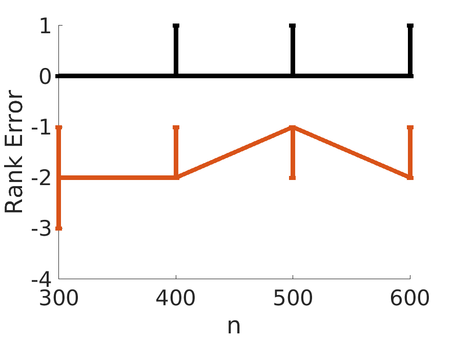
Figure S.1. A comparison of different rank estimators when $p/n=1$, where we show $\widehat{r}^{+}-r^{+}$. The black (red and yellow respective) lines are errors of rank estimator from our rank estimator (42) (ScreeNot and TRAD respectively). The one-sided noises are shown in the first row, where from left to right are the results when $D_{A}$ follows Mix2, Unif[1,10], and Fisher3n respectively. The two-sided noises are shown in the second row, where from left to right are the results when $D_{A}$ and $D_{B}$ follow Mix2 and Unif[1,10], Mix2 and Fisher3n, and Unif[1,10] and Fisher3n respectively. If the corresponding error ratio is too high, the associated curve is not totally plotted to enhance the visualization.

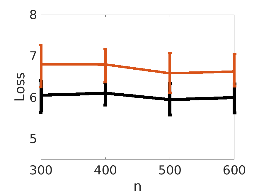
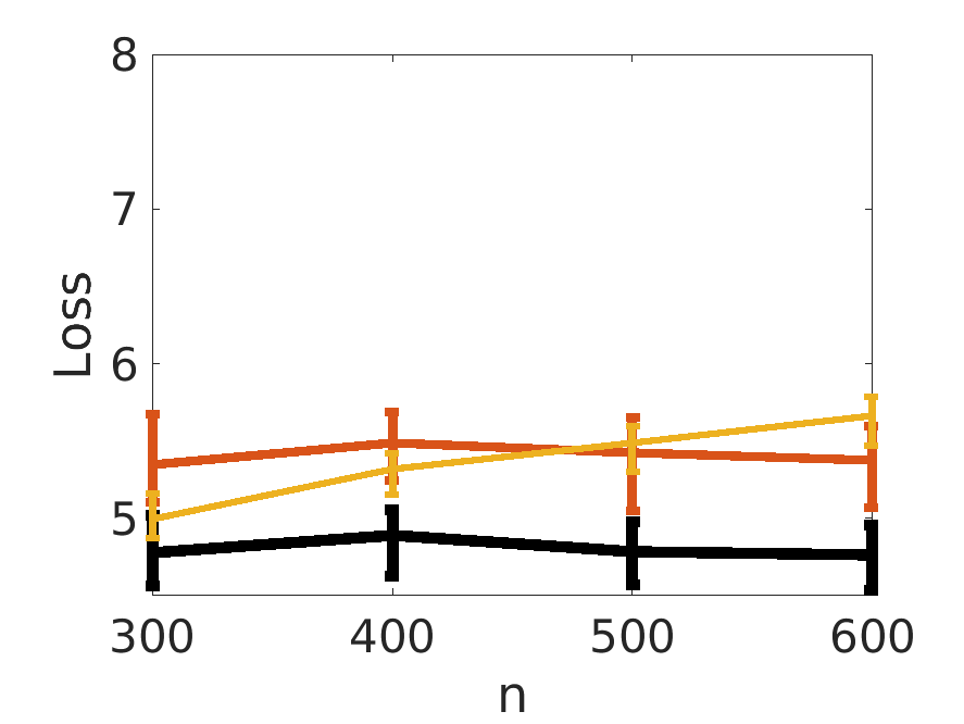
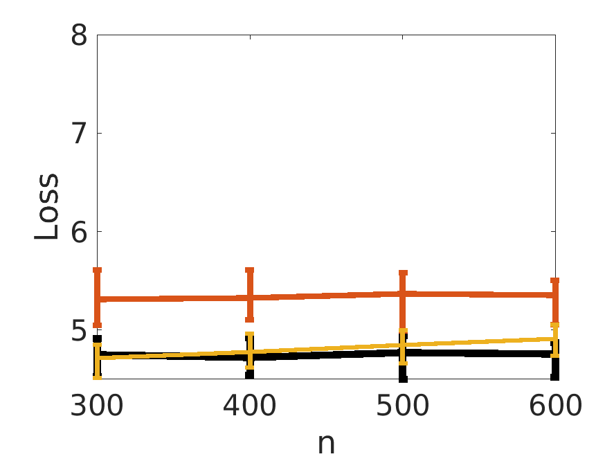
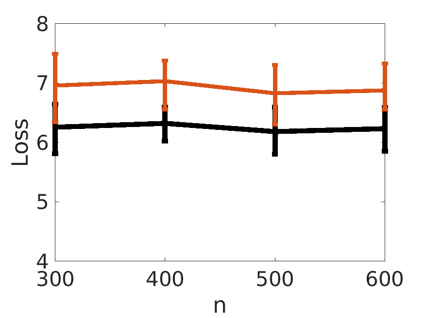
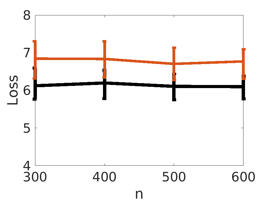
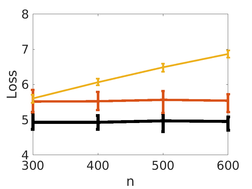
Figure S.2. The Frobenius norm error of different algorithms. The black, red and yellow lines are for eOptShrink, ScreeNOT and TRAD respectively. The one-sided noises are shown in the first row, where from left to right are the results when $D_{A}$ follows Mix2, Unif[1,10], and Fisher3n respectively. The two-sided noises are shown in the second row, where from left to right are the results when $D_{A}$ and $D_{B}$ follow Mix2 and Unif[1,10], Mix2 and Fisher3n, and Unif[1,10] and Fisher3n respectively. If the corresponding error ratio is too high, the associated curve is not totally plotted to enhance the visualization.

In Figure S.3 and S.4, we compare the error ratio of estimating $d_{\min\{r^{+},\widehat{r}^{+}\}}$ and $\sqrt{a_{1,\min\{r^{+},\widehat{r}^{+}\}}a_{2,\min\{r^{+},\widehat{r}^{+}\}}}$ with different pseudo distributions as that in Section 5.1.4 for different combinations of $A$ and $B$. We fix $n=600$ and $p/n=1$. The black, yellow, and red lines indicate the estimator using $\widehat{F}_{\texttt{e}}(x)$, $\widehat{F}_{\texttt{T}}(x)$, and $\widehat{F}_{\texttt{imp}}(x)$ respectively. Clearly, our $\widehat{F}_{\texttt{e}}(x)$ always has a lower error ratio over every $\widehat{r}^{+}$ with statistical significance over every $\widehat{r}^{+}$ while comparing each estimator. This result shows that eOptShrink is robust to a slightly erroneous rank estimation.

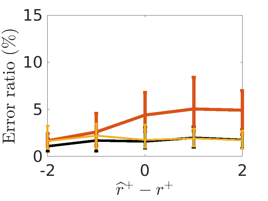
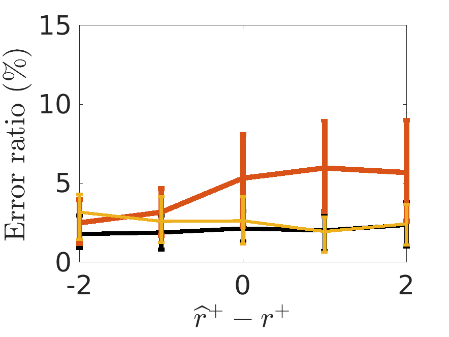
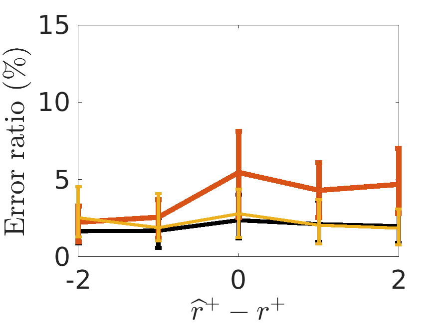
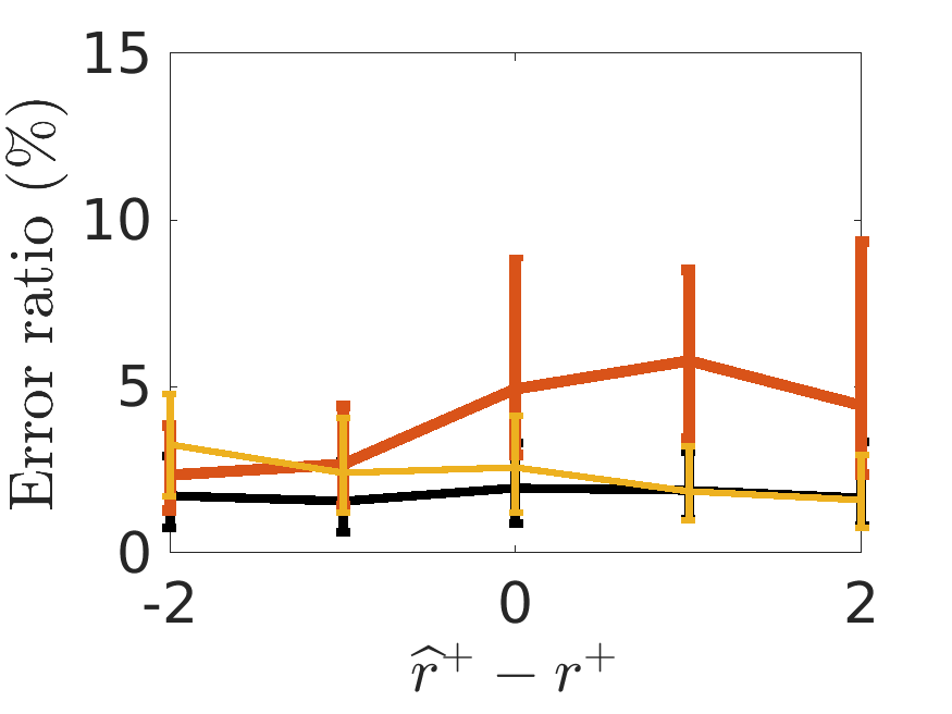
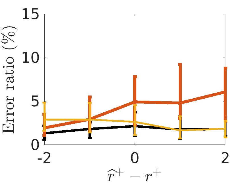
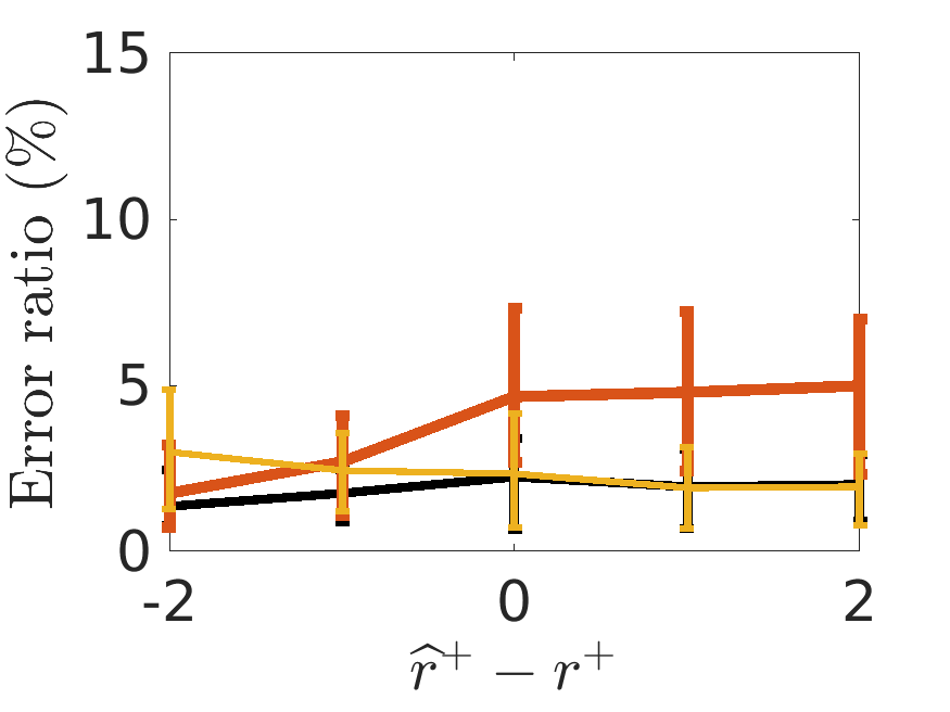
Figure S.3. Interquartile errorbars of error ratios of estimating $d_{\min\{r^{+},\widehat{r}^{+}\}}$ using $\widehat{F}_{\texttt{e}}(x)$, $\widehat{F}_{\texttt{T}}(x)$, and $\widehat{F}_{\texttt{imp}}(x)$, shown in black, yellow and red lines respectively. The one-sided noises are shown in the first row, where from left to right are the results when $D_{A}$ follows Mix2, Unif[1,10], and Fisher3n respectively. The two-sided noises are shown in the second row, where from left to right are the results when $D_{A}$ and $D_{B}$ follow Mix2 and Unif[1,10], Mix2 and Fisher3n, and Unif[1,10] and Fisher3n respectively. We fix $n=600$ and $p/n=1$.

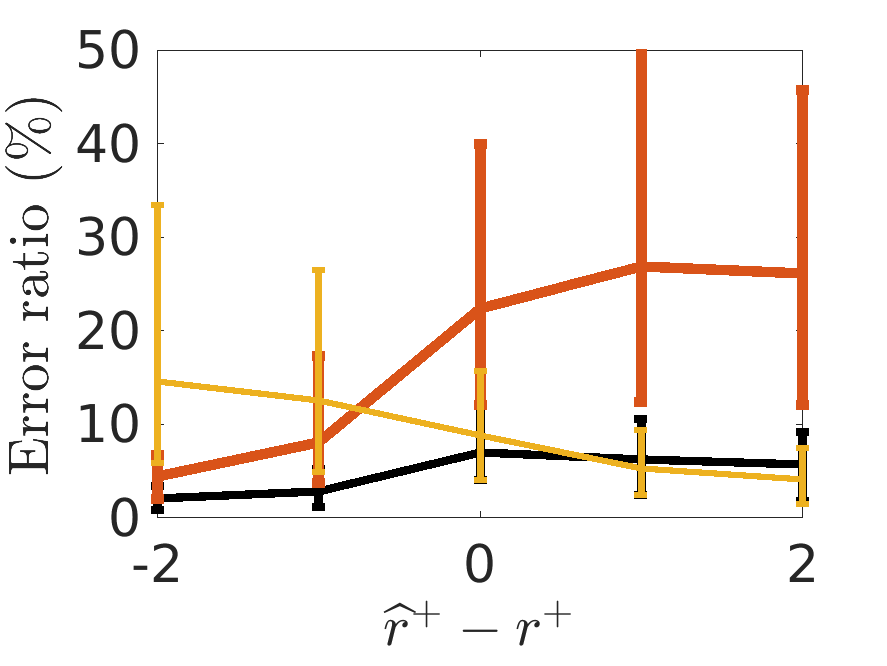
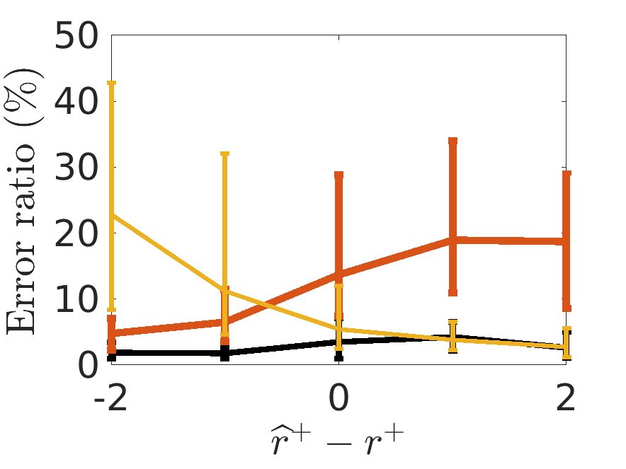
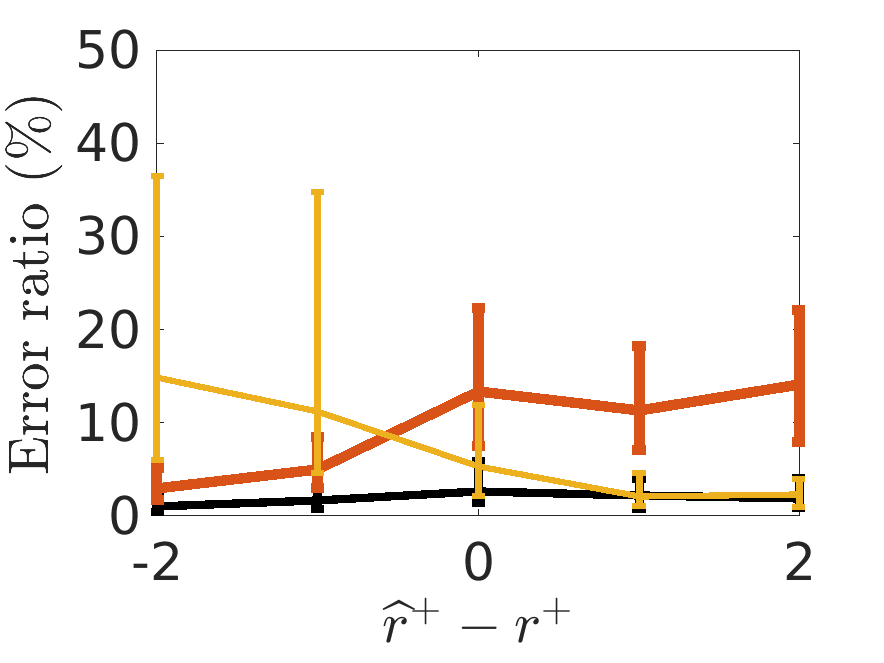
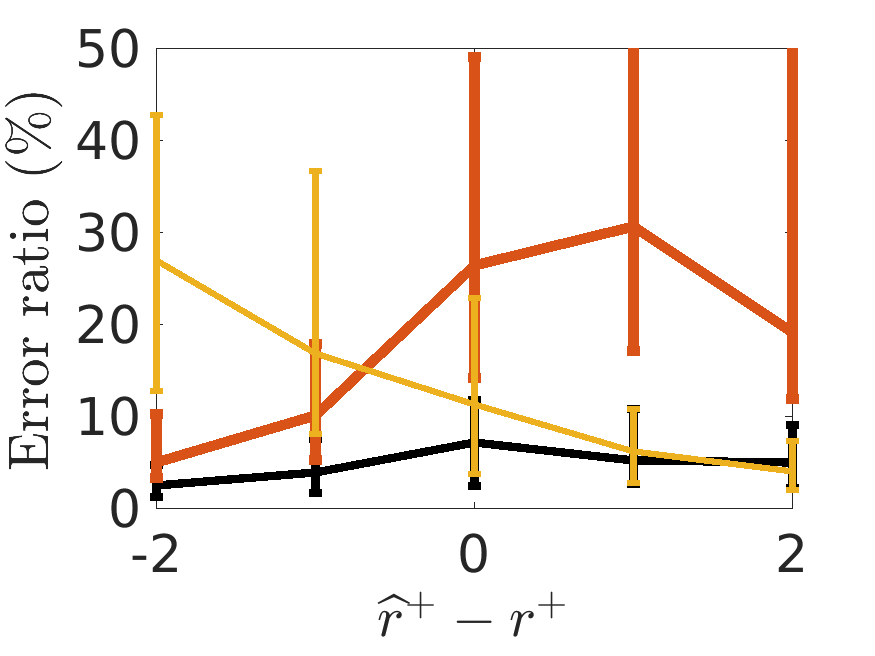
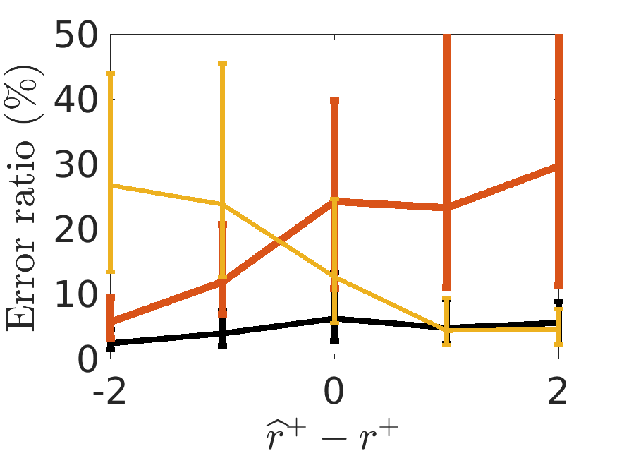
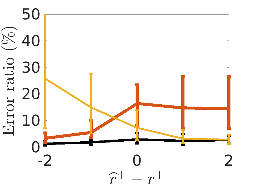
Figure S.4. Interquartile errorbars of error ratios of estimating $\sqrt{a_{1,\min\{r^{+},\widehat{r}^{+}\}}a_{2,\min\{r^{+},\widehat{r}^{+}\}}}$ using $\widehat{F}_{\texttt{e}}(x)$, $\widehat{F}_{\texttt{T}}(x)$, and $\widehat{F}_{\texttt{imp}}(x)$, shown in black, yellow and red lines respectively. The one-sided noises are shown in the first row, where from left to right are the results when $D_{A}$ follows Mix2, Unif[1,10], and Fisher3n respectively. The two-sided noises are shown in the second row, where from left to right are the results when $D_{A}$ and $D_{B}$ follow Mix2 and Unif[1,10], Mix2 and Fisher3n, and Unif[1,10] and Fisher3n respectively. We fix $n=600$ and $p/n=1$.

Appendix S.2 Background knowledge

S.2.1. Some linear algebra tools

We recall a perturbation bound for determinants.

Lemma S.2.1.

Let $A$ and $E$ be two $m\times m$ matrices, where $\sigma_{1}\geq\sigma_{2}\geq\cdots\geq\sigma_{m}$ are singular values of $A$. Then

$$|\det(A+E)-\det(A)|\leq\sum_{i=1}^{m}s_{m-i}\left\lVert E\right\rVert^{i}_{2}\,,$$

where $s_{k}:=\sum_{1\leq i_{1}<i_{2}<\cdots<i_{k}\leq m}\sigma_{i_{1}}\cdots\sigma_{i_{k}}$ is the $k$-th elementary symmetric functions of singular values of $A$ and $s_{0}:=1$.

Lemma S.2.2.

For any $a,b,\alpha_{1},\ldots,\alpha_{r}\in\mathbb{R}$ and $r\in\mathbb{N}$, we have

(S.2.1) $$\det\begin{pmatrix}aI_{r}&\textup{diag}\{\alpha_{1},\cdots,\alpha_{r}\}\\ \textup{diag}\{\alpha_{1},\cdots,\alpha_{r}\}&bI_{r}\end{pmatrix}=\prod_{i=1}^{r}(ab-\alpha_{i}^{2})\,.$$

Further, we summarize the Weyl’s inequality for the singular values of rectangular matrix.

Lemma S.2.3.

For any $p\times n$ matrices $A$ and $B,$ denote $\sigma_{i}(A)$ as the $i$-th largest singular value of $A$. Then we have

$$\sigma_{i+j-1}(A+B)\leq\sigma_{i}(A)+\sigma_{j}(B),\ 1\leq i,j,i+j-1\leq p\wedge n.$$

Lemma S.2.4.

[10, Lemma F.5] Let $z=E+i\eta\in\mathbb{C}^{+}$. For $n\times n$ Hermitian matrices $A$ and $\widetilde{A}$, denote $s(z)$ and $\widetilde{s}(z)$ to be the Stieltjes transforms of their ESD’s. Then we have

(S.2.2) $$|s(z)-\widetilde{s}(z)|\leq\frac{\texttt{rank}(A-\widetilde{A})}{n}\left(\frac{2}{\eta}\wedge\frac{\|A-\widetilde{A}\|}{\eta^{2}}\right)\,.$$

Lemma S.2.5.

[9, Proposition 6.2] Take a measure $\nu$ satisfying the Assumption 2.3(v). Then there exists a constant $c>0$ so that for any matrix $A:=(a_{jk})_{1\leq j,k\leq n}$ with complex entries, any $\delta>0$, and any $g=(g_{1},\ldots,g_{n})^{\top}$ with i.i.d. entries with law $\nu$, we have

$$\mathbb{P}\left(|\langle g,Ag\rangle-\mathbb{E}\langle g,Ag\rangle|>\delta\right)\leq 4e^{-c\left(\frac{\delta}{C}\wedge\frac{\delta^{2}}{C^{2}}\right)}\,,$$

where $C=\sqrt{\operatorname{Tr}(AA^{\top})}$.

S.2.2. Some complex analysis tools

We first provide the following lemma, which is similar to Lemma 2.6 of [58].

Lemma S.2.6.

Assume Assumption 2.3 holds. Then there exist constants $c_{1},c_{2}>0$ such that for $x\in\mathbb{R}$ and $x\downarrow 0$, we have

(S.2.3) $$\rho_{1c}(\lambda_{+}-x)=c_{1}x^{1/2}+\operatorname{O}(x)\ \mbox{ and }\ \rho_{2c}(\lambda_{+}-x)=c_{2}x^{1/2}+\operatorname{O}(x)\,,$$

and for $z\in\mathbb{C}^{+}$ and $z\to\lambda_{+}$, we have

$$\quad m_{1c}(z) \,=m_{1c}(\lambda_{+})+\pi c_{1}(z-\lambda_{+})^{1/2}+\operatorname{O}(|z-\lambda_{+}|)\,,$$

(S.2.4) $$\quad m_{2c}(z) \,=m_{2c}(\lambda_{+})+\pi c_{2}(z-\lambda_{+})^{1/2}+\operatorname{O}(|z-\lambda_{+}|)\,,$$

where $(z-\lambda_{+})^{1/2}$ is taken with the positive imaginary part as the branch cut (the same convention holds in the following). These estimates also hold for $\varrho_{1c}$, $\varrho_{2c}$, $\mathsf{m}_{1c}$ and $\mathsf{m}_{2c}$ with different constants. Moreover, there exists a constant $c_{\mathcal{T}}>0$ such that for $z\in\mathbb{C}^{+}$ and $z\to\lambda_{+}$, we have

(S.2.5) $$\mathcal{T}(z)=\mathcal{T}(\lambda_{+})+\pi c_{\mathcal{T}}(z-\lambda_{+})^{1/2}+\operatorname{O}(|z-\lambda_{+}|)\,.$$

Proof.

Equations (S.2.3) and (S.2.6) are directly from Lemma 2.6 of [58]. By (S.2.6) and the definition of $\mathcal{T}$ in (13), we obtain (S.2.5). ∎

For some properly chosen constants $\varsigma_{1}>0$ and $\varsigma_{2}>1$, we denote the domain of the spectral parameter $z$ as

(S.2.6) $$S(\varsigma_{1},\varsigma_{2}):=\{z=E+i\eta:\lambda_{+}-\varsigma_{1}\leq E\leq\varsigma_{2}\lambda_{+},\,0<\eta\leq 1\}\,.$$

Moreover, for any $z=E+i\eta$, denote

(S.2.7) $$\kappa_{z}:=|E-\lambda_{+}|.$$

The following lemma is similar to Lemma 3.4 in [58] and Lemma S.3.5 in [18].

Lemma S.2.7.

Suppose Assumption 2.3 holds. Then we have

1. for $z\in S(\varsigma_{1},\varsigma_{2})$,

   (S.2.8) $$|\mathcal{T}(z)|\asymp|m_{1c}(z)|\asymp|m_{2c}(z)|\asymp 1\,,$$

   $$\textup{Im }\mathcal{T}(z)\asymp\textup{Im }m_{1c}(z)\asymp\textup{Im }m_{2c}(z)\asymp\begin{cases}\frac{\eta}{\sqrt{\kappa_{z}+\eta}}&\textup{if }E\geq\lambda_{+}\\ \sqrt{\kappa_{z}+\eta}&\textup{if }E\leq\lambda_{+}\,,\end{cases}$$

   and

   $$|\textup{Re }\mathcal{T}(z)-\mathcal{T}(\lambda_{+})| \,\asymp|\textup{Re }m_{1c}(z)-m_{1c}(\lambda_{+})|\asymp|\textup{Re }m_{2c}(z)-m_{2c}(\lambda_{+})|$$

   (S.2.9) $$\,\asymp\begin{cases}\sqrt{\kappa_{z}+\eta},&\textup{if }E\geq\lambda_{+}\\ \frac{\eta}{\sqrt{\kappa_{z}+\eta}}+\kappa_{z},&\textup{if }E\leq\lambda_{+}\,.\end{cases}$$

   The estimates (S.2.8)-(S.2.9) hold for $\varrho_{1c}$, $\varrho_{2c}$, $\mathsf{m}_{1c}$ and $\mathsf{m}_{2c}$.

2. there exists constant $\tau^{\prime}>0$ such that for any $z\in S(\varsigma_{1},\varsigma_{2})$,

   (S.2.10) $$\min_{j=1,\ldots,n}|1+\mathsf{m}_{1c}(z)\sigma_{j}^{b}|\geq\tau^{\prime}\ \ \mbox{and}\ \ \min_{i=1,\ldots,p}|1+\mathsf{m}_{2c}(z)\sigma_{i}^{a}|\geq\tau^{\prime}\,,$$

   where $\sigma_{i}^{a}$ and $\sigma_{j}^{b}$ are eigenvalues of $A$ and $B$ stated in Assumption 2.3.

The above estimates (i)-(ii) hold for $z$ on the real axis, $i.e.,z\in\overline{S(\varsigma_{1},\varsigma_{2})}$.

Proof.

The estimates for $m_{1c}$ and $m_{2c}$ have been proved in Lemma S.3.5 in [18]. Estimates for $\mathcal{T}$ in (S.2.8) and (S.2.9) can be directly derived from (S.2.5), and we omit details. ∎

The following lemma describes the behavior of $\theta$ and the derivatives of $m_{1c}$, $m_{2c}$ and $\mathcal{T}$ on the real line.

Lemma S.2.8.

Suppose Assumption 2.3 holds. For $d\geq\alpha$, we have

(S.2.11) $$|\theta(d)-\lambda_{+}|\asymp(d-\alpha)^{2}.$$

For $x>\lambda_{+}$, we have

(S.2.12) $$m^{\prime}_{1c}(x)\asymp\kappa_{x}^{-1/2},\quad m^{\prime}_{2c}(x)\asymp\kappa_{x}^{-1/2}\ \mbox{ and }\ \mathcal{T}^{\prime}(x)\asymp\kappa_{x}^{-1/2}\,.$$

Proof.

With (S.2.5), we obtain that

$$d_{i}^{-2}=\mathcal{T}(\theta(d_{i}))=\alpha^{-2}+C\sqrt{\theta(d_{i})-\lambda_{+}}+\operatorname{O}(|\theta(d_{i})-\lambda_{+}|)$$

if $\theta(d_{i})-\lambda_{+}\leq\varsigma_{1}$ for some sufficiently small constant $0<\varsigma_{1}<1$, and

$$d_{i}^{-2}=\mathcal{T}(\theta(d_{i}))\geq\mathcal{T}(\lambda_{+}+\varsigma_{1})=\alpha^{-2}+C\sqrt{\varsigma_{1}}+\operatorname{O}(\varsigma_{1})$$

if $\theta(d_{i})-\lambda_{+}\geq\varsigma_{1}$, where in the inequality we use the fact that $\mathcal{T}(x)$ is monotone increasing when $x>\lambda_{+}.$ The above two estimates imply (S.2.11). The first two statements of (S.2.12) have been proved in Lemma S.3.6 in [18], and the third statement then can be derived by

$$\mathcal{T}^{\prime}(x) \,=m_{1c}(x)m_{2c}(x)+xm^{\prime}_{1c}(x)m_{2c}(x)+xm_{1c}(x)m^{\prime}_{2c}(x)$$

(S.2.13) $$\,\asymp C_{1}+C_{2}\kappa_{x}^{-1/2}\asymp\kappa_{x}^{-1/2},$$

where we used the first statement of (S.2.12) and (S.2.8) in the first $\asymp$ and the fact that $\kappa_{x}^{-1/2}$ blows up when $x\to\lambda_{+}$ in the last approximation. ∎

Note that by (S.2.11) and (S.2.12), for $d\geq\alpha$, we have

(S.2.14) $$m_{1c}^{\prime}(\theta(d))\asymp\frac{1}{d-\alpha},\quad m_{2c}^{\prime}(\theta(d))\asymp\frac{1}{d-\alpha},\quad\mathcal{T}^{\prime}(\theta(d))\asymp\frac{1}{d-\alpha}$$

and

(S.2.15) $$\theta^{\prime}(d)\asymp d-\alpha\,.$$

Lemma S.2.9.

Suppose Assumption 2.3 holds. Then for any constant $\varsigma>\lambda_{+}$, there exist constants $\tau_{1},\tau_{2}>0$ such that the following statements hold.

1. $\mathcal{T}$ is a holomorphic homeomorphism on the spectral domain

   (S.2.16) $$\mathbf{D}_{1}(\tau_{1},\varsigma):=\{z=E+i\eta:\lambda_{+}<E<\varsigma,\,-\tau_{1}<\eta<\tau_{1}\}.$$

   As a consequence, the inverse of $\mathcal{T}$ exists and we denote it by $\theta$.

2. $\theta$ is holomorphic homeomorphism on $\mathbf{D}_{2}(\tau_{2},\varsigma)$, where

   (S.2.17) $$\mathbf{D}_{2}(\tau_{2},\varsigma):=\{\zeta=E+i\eta:\alpha<E<1/\sqrt{\mathcal{T}(\varsigma)},\,-\tau_{2}<\eta<\tau_{2}\},$$

   such that $\mathbf{D}_{2}(\tau_{2},\varsigma)\subset 1/\sqrt{\mathcal{T}(\mathbf{D}_{1}(\tau_{1},\varsigma))}$.

3. For $z\in\mathbf{D}_{1}(\tau_{1},\varsigma)$, we have

   (S.2.18) $$|\mathcal{T}(z)-\mathcal{T}(\lambda_{+})|\asymp|z-\lambda_{+}|^{1/2}\ \mbox{ and }\ |\mathcal{T}^{\prime}(z)|\asymp|z-\lambda_{+}|^{-1/2}.$$

4. For $\zeta\in\mathbf{D}_{2}(\tau_{2},\varsigma)$, we have

   (S.2.19) $$|\theta(\zeta)-\lambda_{+}|\asymp|\zeta-\alpha|^{2}\ \mbox{ and }\ |\theta^{\prime}(\zeta)|\asymp|\zeta-\alpha|.$$

5. For $z_{1},z_{2}\in\mathbf{D}_{1}(\tau_{1},\varsigma)$ and $w_{1},w_{2}\in\mathbf{D}_{2}(\tau_{2},\varsigma)$, we have

   (S.2.20) $$|\mathcal{T}(z_{1})-\mathcal{T}(z_{2})|\asymp\frac{|z_{1}-z_{2}|}{\max_{i=1,2}|z_{i}-\lambda_{+}|^{1/2}},$$

   and

   (S.2.21) $$|\theta(w_{1})-\theta(w_{2})|\asymp|w_{1}-w_{2}|\cdot\max_{i=1,2}|w_{i}-\alpha|.$$

Note that in (24), $\theta$ is only defined on the real line, but in Lemma S.2.9(i), we extend its definition to the complex plane. The relationship between $\theta$ and $\mathcal{T}$ is summarized in Figure S.5.

Proof.

Similar results for $m_{1c}$ and $m_{2c}$ and their proofs can be found in [18, Lemma S.3.7]. We derive this Lemma specifically using the definition of $\mathcal{T}(z)$ and $\theta(\zeta)$ with the same approach, and we omit the detail here. ∎

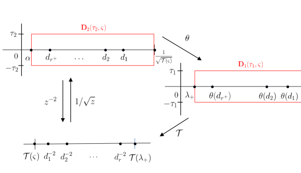
Figure S.5. An illustration of the relationship of $\mathcal{T}$, $\theta$ and several quantities used in the proof. Note that $\theta(\alpha)=\lambda_{+}$.

S.2.3. Some random matrix tools

We record some results from the random matrix theorem that we will repeatedly apply in the following proofs. Recall that the eigenvalues of $ZZ^{\top}$ are $\lambda_{1}\geq\lambda_{2}\geq\cdots\geq\lambda_{p\wedge n}$.

Denote

(S.2.22) $$\Psi(z):=\sqrt{\frac{\text{Im }\mathsf{m}_{2c}(z)}{n\eta}}+\frac{1}{n\eta}.$$

Note that for any $z=E+i\eta\in S(\varsigma_{1},\varsigma_{2})$, from (i) of Lemma S.2.7 and (S.2.10), we have [58, (3.19)]

(S.2.23) $$\Psi(z)\gtrsim n^{-1/2},\quad\Psi^{2}(z)\lesssim 1/n\eta,$$

and $\Psi^{2}(E+i\eta)+\phi_{n}/n\eta$ is monotonically decreasing with respect to $\eta$ [58, below Lemma 3.7]. Hence there is a unique $\eta_{l}(E)$ such that

$$n^{1/2}\left[\Psi^{2}(E+i\eta_{l}(E))+\frac{\phi_{n}}{n\eta_{l}(E)}\right]=1.$$

Note that by (S.2.8) and (S.2.22), we have

(S.2.24) $$\eta_{l}(E)\asymp n^{-3/4}+n^{-1/2}\left(\sqrt{\kappa_{E}}+\phi_{n}\right),\quad\text{ for }\ \ E\leq\lambda_{+}\,.$$

For $E>\lambda_{+}$, we define $\eta_{l}(E):=\eta_{l}(\lambda_{+})=\operatorname{O}(n^{-3/4}+n^{-1/2}\phi_{n})$. Then we have the following rigidity result. Recall the definition of classical location $\gamma_{j}$ in (15).

Lemma S.2.10.

(Rigidity of eigenvalues [58, Theorem 3.8]). Suppose Assumption 2.3 holds. Then we have the following estimates for any fixed $0<\varsigma<\varsigma_{1}$, where $\varsigma_{1}$ comes from the definition of $S(\varsigma_{1},\varsigma_{2})$ in (S.2.6). For any $j$ such that $\lambda_{+}-\varsigma\leq\gamma_{j}\leq\lambda_{+}$, we have

(S.2.25) $$|\lambda_{j}-\gamma_{j}|\prec n^{-2/3}\left(j^{-1/3}+\mathbbm{1}(j\leq n^{1/4}\phi_{n}^{3/2})\right)+\eta_{l}(\gamma_{j})+n^{2/3}j^{-2/3}\eta_{l}^{2}(\gamma_{j})\,,$$

where $\eta_{l}(\gamma_{j}){\asymp n^{-3/4}+n^{-5/6}j^{1/3}+n^{-1/2}\phi_{n}}$. Moreover, if either $A$ or $B$ is diagonal, the bound (S.2.25) is improved to

(S.2.26) $$|\lambda_{j}-\gamma_{j}|\prec n^{-2/3}j^{-1/3}.$$

Also, we have the delocalization result for eigenvectors.

Lemma S.2.11.

(Isotropic delocalization of eigenvectors [18, Lemma S.3.13]) Suppose Assumption 2.3 hold. Then we have the following estimates for any fixed constant $0<\varsigma<\varsigma_{1}$. For any deterministic unit vectors $\mathbf{u}\in\mathbb{C}^{p}$ and $\mathbf{v}\in\mathbb{C}^{n}$, we have

(S.2.27) $$\left|\langle\mathbf{u},{\xi}_{k}\rangle\right|^{2}+\left|\langle\mathbf{v},{\zeta}_{k}\rangle\right|^{2}\prec n^{-1}+\eta_{l}(\gamma_{k})\left(\frac{k}{n}\right)^{1/3}+\eta_{l}(\gamma_{k})\phi_{n},$$

for all $k$ such that $\lambda_{+}-\varsigma\leq\gamma_{k}\leq\lambda_{+}$, where $\eta_{l}(\gamma_{k})=\operatorname{O}(n^{-3/4}+n^{-5/6}k^{1/3}+\phi_{n}n^{-1/2})$. If the extra assumptions for (30) in Theorem 3.3 hold, we have

(S.2.28) $$\max_{k:\lambda_{+}-\varsigma\leq\gamma_{k}\leq\lambda_{+}}\left\{\left|\langle\mathbf{u},{\bm{\xi}}_{k}\rangle\right|^{2}+\left|\langle\mathbf{v},{\bm{\zeta}}_{k}\rangle\right|^{2}\right\}\prec n^{-1}.$$

Next, we discuss some properties of resolvents and local laws. For any $z\in\mathbb{C}^{+},$ denote

$$H:=H(z):=\begin{pmatrix}0&{z^{1/2}}Z\\ z^{1/2}Z^{\top}&0\end{pmatrix}\in\mathbb{C}^{(p+n)\times(p+n)}$$

and

(S.2.29) $$\widetilde{H}:=\widetilde{H}(z):=\begin{pmatrix}0&z^{1/2}\widetilde{S}\\ z^{1/2}\widetilde{S}^{\top}&0\end{pmatrix}\in\mathbb{C}^{(p+n)\times(p+n)},$$

where $z^{1/2}$ is defined with the positive imaginary part as the branch cut. Note that we have

(S.2.30) $$\widetilde{H}(z)=\begin{pmatrix}0&z^{1/2}Z\\ z^{1/2}Z^{\top}&0\end{pmatrix}+\begin{pmatrix}0&z^{1/2}S\\ z^{1/2}S^{\top}&0\end{pmatrix}=H(z)+\mathbf{U}\mathbf{D}\mathbf{U}^{\top},$$

where

(S.2.31) $$\mathbf{D}=\begin{pmatrix}0&{z^{1/2}}D\\ z^{1/2}D&0\end{pmatrix}\in{\mathbb{C}^{2r\times 2r}}\ \mbox{ and }\ \mathbf{U}=\begin{pmatrix}U&0\\ 0&V\end{pmatrix}\in\mathbb{R}^{(p+n)\times 2r}$$

such that $D=\textup{diag}\{d_{1},\cdots,d_{r}\}\in\mathbb{R}^{r\times r}$ is a diagonal matrix formed by singular values, and $U=(\mathbf{u}_{1},\cdots,\mathbf{u}_{r})\in\mathbb{R}^{p\times r}$ and $V=(\mathbf{v}_{1},\cdots,\mathbf{v}_{r})\in\mathbb{R}^{n\times r}$ are matrices formed by left and right singular vectors defined in (1). The eigenvalues of $\widetilde{H}$ coincide with the singular values of $z^{1/2}\widetilde{S}.$ Therefore, it suffices to study the matrix $\widetilde{H}$. Further, we denote the Green functions of $H$ and $\widetilde{H}$ respectively as

$$G:=G(z):=(H-z)^{-1}\ \mbox{ and }\ \widetilde{G}:=\widetilde{G}(z):=(\widetilde{H}-z)^{-1}\,,$$

where $z\in\mathbb{C}^{+}$. By the Schur’s complement, we have

(S.2.34) $$G(z) \,=\left({\begin{array}[]{*{20}c}{\mathcal{G}_{1}(z)}&z^{-1/2}\mathcal{G}_{1}(z)Z\\ z^{-1/2}Z^{\mathrm{T}}\mathcal{G}_{1}(z)&\mathcal{G}_{2}(z)\\ \end{array}}\right)$$

(S.2.37) $$\widetilde{G}(z) \,=\left({\begin{array}[]{*{20}c}{\widetilde{\mathcal{G}}_{1}(z)}&z^{-1/2}\widetilde{\mathcal{G}}_{1}(z)Z\\ z^{-1/2}Z^{\mathrm{T}}\widetilde{\mathcal{G}}_{1}(z)&\widetilde{\mathcal{G}}_{2}(z)\\ \end{array}}\right),$$

where $\mathcal{G}_{1}$ and $\mathcal{G}_{2}$ are defined in (5). Further, by the spectral decomposition, we have

(S.2.40) $${G}(z)=\sum_{k=1}^{p\wedge n}\frac{1}{{\lambda}_{k}-z}\left({\begin{array}[]{*{20}c}{{\bm{\xi}}_{k}{\bm{\xi}}^{\top}_{k}}&z^{-1/2}\sqrt{{\lambda}}_{k}{\bm{\xi}}_{k}{\bm{\zeta}}_{k}^{\top}\\ z^{-1/2}\sqrt{{\lambda}}_{k}{\bm{\zeta}}_{k}{\bm{\xi}}_{k}^{\top}&{\bm{\zeta}}_{k}{\bm{\zeta}}_{k}^{\top}\\ \end{array}}\right)\in\mathbb{C}^{(p+n)\times(p+n)}$$

(S.2.43) $$\widetilde{G}(z)=\sum_{k=1}^{p\wedge n}\frac{1}{{\widetilde{\lambda}}_{k}-z}\left({\begin{array}[]{*{20}c}{{\widetilde{\bm{\xi}}}_{k}{\widetilde{\bm{\xi}}}^{\top}_{k}}&z^{-1/2}\sqrt{{\widetilde{\lambda}}}_{k}{\widetilde{\bm{\xi}}}_{k}{\widetilde{\bm{\zeta}}}_{k}^{\top}\\ z^{-1/2}\sqrt{{\widetilde{\lambda}}}_{k}{\widetilde{\bm{\zeta}}}_{k}{\widetilde{\bm{\xi}}}_{k}^{\top}&{\widetilde{\bm{\zeta}}}_{k}{\widetilde{\bm{\zeta}}}_{k}^{\top}\\ \end{array}}\right)\in\mathbb{C}^{(p+n)\times(p+n)}\,.$$

The following lemma characterizes the locations of the outlier eigenvalues of $\widetilde{H}$.

Lemma S.2.12.

[30, Lemma 6.1] Assume $\mu\in\mathbb{R}-\text{Spec}(H)$. Then $\mu\in\text{Spec}(\widetilde{H})$ if and only if

(S.2.44) $$\det(\mathbf{U}^{\top}G(\mu)\mathbf{U}+\mathbf{D}^{-1})=0\,.$$

Next lemma provides a link between the Green functions $G(z)$ and $\widetilde{G}(z).$ The proof is straightforward depending on the Woodbury formula and the basic identity $A-A(A+B)^{-1}A=B-B(A+B)^{-1}B$ when $A$, $B$ and $A+B$ are all invertible.

Lemma S.2.13.

[15, Lemma 4.8] For $z\in\mathbb{C}^{+},$ we have

(S.2.45) $$\widetilde{G}(z)=G(z)-G(z)\mathbf{U}(\mathbf{D}^{-1}+\mathbf{U}^{\top}G(z)\mathbf{U})^{-1}\mathbf{U}^{\top}G(z)\,.$$

This lemma immediately leads to the following relationship.

(S.2.46) $$\mathbf{U}^{\top}\widetilde{G}(z)\mathbf{U}=\mathbf{D}^{-1}-\mathbf{D}^{-1}(\mathbf{D}^{-1}+\mathbf{U}^{\top}G(z)\mathbf{U})^{-1}\mathbf{D}^{-1}.$$

Next, for any $z\in\mathbb{C}^{+}$, denote

(S.2.47) $$\Pi(z):=\left({\begin{array}[]{*{20}c}{\Pi_{1}}(z)&0\\ 0&{\Pi_{2}}(z)\\ \end{array}}\right)\in\mathbb{C}^{(p+n)\times(p+n)},$$

where

$$\Pi_{1}(z):=-z^{-1}\left(1+\mathsf{m}_{2c}(z)A\right)^{-1}\ \mbox{ and }\ \Pi_{2}(z):=-z^{-1}(1+\mathsf{m}_{1c}(z)B)^{-1}.$$

Denote

(S.2.48) $$\overline{\Pi}(z):=\begin{pmatrix}m_{1c}(z)I_{r}&0\\ 0&m_{2c}(z)I_{r}\end{pmatrix}\in\mathbb{C}^{2r\times 2r}.$$

Note that $\Pi(z)$ and $\overline{\Pi}(z)$ are related via $m_{1c}(z)=\frac{1}{p}\operatorname{Tr}{\Pi_{1}}(z)$ and $m_{2c}(z)=\frac{1}{n}\operatorname{Tr}{\Pi_{2}}(z)$, and we will show below the relationship between $\Pi(z)$ and $\overline{\Pi}(z)$ and how $\mathbf{U}^{\top}\Pi(z)\mathbf{U}$ converges to $\overline{\Pi}(z)$. We denote the difference

(S.2.49) $$\Omega(z):=\mathbf{U}^{\top}G(z)\mathbf{U}-\overline{\Pi}(z)\,,$$

which will be used to control the noise part in the analysis. With $\Omega(z)$, we have the following identity

(S.2.50) $$(\mathbf{D}^{-1}+\mathbf{U}^{\top}G(z)\mathbf{U})^{-1}=(\mathbf{D}^{-1}+\overline{\Pi}(z))^{-1}+(\mathbf{D}^{-1}+\overline{\Pi}(z))^{-1}\Omega(z)(\mathbf{D}^{-1}+\mathbf{U}^{\top}G(z)\mathbf{U})^{-1}.$$

By iteration, we have the following $\ell$-th resolvent expansion.

Lemma S.2.14.

(Resolvant identity [10]) For $\ell\geq 1$, we have the following $\ell$-th order resolvent expansion:

$$(\mathbf{D}^{-1}+\mathbf{U}^{\top}G(z)\mathbf{U})^{-1}= \sum_{k=0}^{\ell-1}(\mathbf{D}^{-1}+\overline{\Pi}(z))^{-1}[\Omega(z)(\mathbf{D}^{-1}+\overline{\Pi}(z))]^{k}$$

(S.2.51) $$+[(\mathbf{D}^{-1}+\overline{\Pi}(z))^{-1}\Omega(z)]^{\ell}[\mathbf{D}^{-1}+\mathbf{U}^{\top}G(z)\mathbf{U}]^{-1}.$$

We define the following spectral regions. Recall the definition of $S(\varsigma_{1},\varsigma_{2})$ in (S.2.6). Denote the following domains of the spectral parameter $z$ as

$$S_{0}(\varsigma_{1},\varsigma_{2},\omega):= \,S(\varsigma_{1},\varsigma_{2})\cap\{z=E+i\eta:\eta\geq n^{-1+\omega}\}\,,$$

(S.2.52) $$\widetilde{S}_{0}(\varsigma_{1},\varsigma_{2},\omega):= \,S_{0}(\varsigma_{1},\varsigma_{2},\omega)\cap\left\{z=E+i\eta:n^{1/2}\left(\Psi^{2}(z)+\frac{\phi_{n}}{n\eta}\right)\leq n^{-\omega/2}\right\}$$

and

(S.2.53) $$S_{out}(\varsigma_{2},\omega):=\{E+i\eta:\lambda_{+}+n^{\omega}(n^{-2/3}+n^{-1/3}\phi_{n}^{2})\leq E\leq\varsigma_{2}\lambda_{+},\eta\in[0,1]\}.$$

Inside these domains, we have the following local laws.

Theorem S.2.15.

(Local laws “near” $\lambda_{+}$ [18, Theorem S.3.9]). Suppose that Assumption 2.3 holds. Fix constant $\varsigma_{1}>0$ and $\varsigma_{2}>1$ as those in Lemma S.2.7. Then for any fixed $\epsilon>0$, the following estimates hold.

1. Anisotropic local law: For any $z\in\widetilde{S}_{0}(\varsigma_{1},\varsigma_{2},\omega)$ and deterministic unit vectors $\bm{\mu},\bm{\nu}\in\mathbb{C}^{p+n}$, we have

   (S.2.54) $$\left|\langle\bm{\mu},(G(z)-\Pi(z))\bm{\nu}\rangle\right|\prec\phi_{n}+\Psi(z).$$

2. Averaged local law: For any $z\in\widetilde{S}_{0}(\varsigma_{1},\varsigma_{2},\omega)$, we have

   (S.2.55) $$|m_{1}(z)-m_{1c}(z)|+|m_{2}(z)-m_{2c}(z)|\prec(n\eta)^{-1}.$$

   Moreover, when $z\in\widetilde{S}_{0}(\varsigma_{1},\varsigma_{2},\omega)\cap\{z=E+i\eta:E\geq\lambda_{+},n\eta\sqrt{\kappa_{z}+\eta}\geq{n^{\omega}}\}$, we have the following stronger estimate

   (S.2.56) $$|m_{1}(z)-m_{1c}(z)|+|m_{2}(z)-m_{2c}(z)|\prec\frac{n^{-\omega/4}}{n\eta}+\frac{1}{n(\kappa_{z}+\eta)}+\frac{1}{(n\eta)^{2}\sqrt{\kappa_{z}+\eta}},$$

   which is uniformly on $z$.

Note that the term “anisotropic” means that the resolvent $G(z)$ is well approximated by a deterministic matrix that is not a multiple of an identity matrix.

Theorem S.2.16.

(Anisotropic local law beyond $\lambda_{+}$ [18, Theorem S.3.12]). Suppose Assumption 2.3 holds. For any $0<\omega<2/3$, $z\in S_{out}(\varsigma_{2},\omega)$ and deterministic unit vectors $\mathbf{v},\mathbf{w}\in\mathbb{C}^{p+n},$ we have

(S.2.57) $$\left|\langle\mathbf{v},(G(z)-\Pi(z))\mathbf{w}\rangle\right|\prec\phi_{n}+\sqrt{\frac{\textup{Im}m_{2c}(z)}{n\eta}}\asymp\phi_{n}+n^{-1/2}(\kappa_{z}+\eta)^{-1/4}.$$

Finally, we derive the following lemma to describe the difference between $\Pi(z)$ and $\overline{\Pi}(z)$ near and beyond $\lambda_{+}$.

Lemma S.2.17.

Under Assumption 2.3, for any $z\in\widetilde{S}_{0}(\varsigma_{1},\varsigma_{2},\omega)\cup S_{out}(\varsigma_{2},\omega)$ and $i,j=1,\ldots,r$, we have

$$|\langle\mathbf{u}_{i},\,z^{-1}(1+ \mathsf{m}_{2c}(z)A)^{-1}\mathbf{u}_{j}\rangle-\delta_{ij}m_{1c}(z)|$$

$$\vee|\langle\mathbf{v}_{i},\,z^{-1}(1+\mathsf{m}_{1c}(z)B)^{-1}\mathbf{v}_{j}\rangle-\delta_{ij}m_{2c}(z)|\prec n^{-1}\,;$$

that is,

(S.2.58) $$\left\lVert\mathbf{U}^{\top}\Pi(z)\mathbf{U}-\overline{\Pi}(z)\right\rVert\prec n^{-1}\,.$$

Proof.

When $z\in\widetilde{S}_{0}(\varsigma_{1},\varsigma_{2},\omega)\cup{S}_{out}(\varsigma_{2},\omega)$, by (10) and Lemma S.2.5, for any $\delta>0$ we have that

$$\mathbb{P}\left(|n\langle\mathbf{u}_{i},\,z^{-1}(1+\mathsf{m}_{2c}(z)A)^{-1}\mathbf{u}_{j}\rangle-\mathbb{\delta}_{ij}\operatorname{Tr}(z^{-1}(1+\mathsf{m}_{2c}(z)A)^{-1})|>\delta\right)$$

$$=\, \mathbb{P}\left(|\langle\mathbf{u}_{i},\,z^{-1}(1+\mathsf{m}_{2c}(z)A)^{-1}\mathbf{u}_{j}\rangle-\mathbb{\delta}_{ij}m_{1c}(z)|>n^{-1}\delta\right)\leq 4e^{-c\left(\frac{\delta}{C}\wedge\frac{\delta^{2}}{C^{2}}\right)}$$

and some constants $c,C>0$, where $n$ is used to normalize $\mathbf{u}_{i}$ and $\mathbf{u}_{j}$ to fit the conditions of $g$ in Lemma S.2.5. Thus, given any small constant $\epsilon>0$ and large constant $D>0$, by letting $\delta=n^{\omega}$, we have

$$\mathbb{P}\left(|\langle\mathbf{u}_{i},z^{-1}(1+\mathsf{m}_{2c}(z)A)^{-1}\mathbf{u}_{j}\rangle-\delta_{ij}m_{1c}(z)|>n^{-1+\epsilon}\right)\leq 4n^{-\frac{cn^{\omega}}{C}}\leq n^{-D}$$

when $n$ is sufficiently large. By a similar approach we have the same control for the other term, and hence the proof. ∎

Appendix S.3 Proof of Theorem 3.2

With Lemmas S.2.10, S.2.15, S.2.16 and S.2.17 and the triangle inequality, for some given fixed small $\epsilon>0,$ we find that there exists an event $\Xi$ of high probability such that the followings hold when conditional on $\Xi$:

1. For $z\in\widetilde{S}_{0}(\varsigma_{1},\varsigma_{2},\epsilon)$, from Lemmas S.2.15 and S.2.17, and since $r$ is bounded, we have that

   (S.3.59) $$\left\lVert\mathbf{U}^{\top}G(z)\mathbf{U}-\overline{\Pi}(z)\right\rVert\leq n^{\epsilon/2}(\phi_{n}+\Psi(z)).$$

2. For $z\in S_{out}(\varsigma_{2},\epsilon),$ from Lemmas S.2.15 and S.2.17, and since $r$ is bounded, we have that

   (S.3.60) $$\left\lVert\mathbf{U}^{\top}G(z)\mathbf{U}-\overline{\Pi}(z)\right\rVert\leq n^{\epsilon/2}(\phi_{n}+n^{-1/2}(\kappa_{z}+\eta)^{-1/4})\,.$$

3. From Lemma S.2.10, there exists a large integer $\varpi$, such that for $1\leq i\leq\varpi,$ we have

   (S.3.61) $$|\lambda_{i}-\lambda_{+}|\leq n^{\epsilon}(n^{-1/3}\phi_{n}^{2}+n^{-2/3})\,,$$

   where $\varpi>r$ is a fixed integer.

Below, the proof is conditional on $\Xi$ such that (S.3.59), (S.3.60) and (S.3.61) hold.

Step I. Find asymptotic outlier locations $\theta(d_{i})$ and the threshold $\alpha$. We start with finding the asymptotic outlier locations for eigenvalues of $\widetilde{S}\widetilde{S}^{\top}$. As is shown in (S.3.60), $\mathbf{U}^{\top}G(z)\mathbf{U}$ converges to $\overline{\Pi}(z)$ in the operator norm for $z\in S_{out}(\varsigma_{2},\epsilon)$. Together with Lemma S.2.12 and the continuity of determinant, $\mu>\lambda_{+}$ is asymptotically an outlier location if and only if

(S.3.62) $$\lim_{n\to\infty}\det(\mathbf{U}^{\top}G(\mu)\mathbf{U}+\mathbf{D}^{-1})=\det\left(\overline{\Pi}(\mu)+\mathbf{D}^{-1}\right)=0$$

By Lemma S.2.2, (S.3.62) becomes

$$\det\left(\overline{\Pi}(\mu)+\mathbf{D}^{-1}\right)=\det\left(\begin{pmatrix}m_{1c}(\mu)I_{r}&0\\ 0&m_{2c}(\mu)I_{r}\end{pmatrix}+\mathbf{D}^{-1}\right)$$

(S.3.63) $$=\, \mu^{-r}\prod_{i=1}^{r}(\mu m_{1c}(\mu)m_{2c}(\mu)-d_{i}^{-2})=\mu^{-r}\prod_{i=1}^{r}(\mathcal{T}(\mu)-d_{i}^{-2})=0\,.$$

By the definition of $\theta(\cdot)$, the determinant is zero when $\mu=\theta(d_{i})$ for $1\leq i\leq r$. Note that since $\mathcal{T}(x)$ is a monotonically decreasing function for $x>\lambda_{+}$, we have $\theta(d_{i})$ as a solution of (S.3) if and only if $d_{i}^{-2}<\lambda_{+}m_{1c}(\lambda_{+})m_{2c}(\lambda_{+})$, which is equivalent to $d_{i}>\alpha$. In other words, $\alpha$ is the desired signal strength threshold.

Step II. Define the permissible intervals for the spectrum. Now the strategy is to prove that with high probability there are no eigenvalues outside a neighbourhood of each $\theta(d_{i})$. Define the index set

(S.3.64) $$\mathbb{O}_{\epsilon}:=\{i:d_{i}-\alpha\geq n^{\epsilon}(\phi_{n}+n^{-1/3})\}=\{1,2,\ldots,r_{\epsilon}\}\subset\mathbb{O}_{+},$$

for some $r_{\epsilon}\leq r^{+}$. This means the signal strength $d_{i}$ is strong enough if $i\in\mathbb{O}_{\epsilon}$. For $1\leq i\leq r$, define the interval

(S.3.65) $$I_{i}:=[\theta(d_{i})-n^{\epsilon}\omega(d_{i}),\,\theta(d_{i})+n^{\epsilon}\omega(d_{i})],$$

where

(S.3.66) $$\omega(d_{i}):=\phi_{n}\Delta(d_{i})^{2}+n^{-1/2}\Delta(d_{i})\,.$$

Also, define

$$I_{0}:=[0,\,\lambda_{+}+n^{3\epsilon}(\phi_{n}^{2}+n^{-2/3})]\quad\mbox{and}\quad I:=I_{0}\cup\bigcup_{i\in\mathbb{O}_{\epsilon}}I_{i}\,.$$

Step III. Show that $I$ contains all eigenvalues of $\widetilde{H}$. By (S.2.49), we have

(S.3.67) $$\mathbf{U}^{\top}G(z)\mathbf{U}+\mathbf{D}^{-1}=\overline{\Pi}(z)+\mathbf{D}^{-1}+\Omega(z)\,.$$

Again, by Lemma S.2.12 and let $z=\mu\in I$ in (S.3.60), where $\mu$ is an eigenvalue of $\widetilde{H}$ if and only if

$$\det(\mathbf{U}^{\top} G(\mu)\mathbf{U}+\mathbf{D}^{-1})=\det(\overline{\Pi}(\mu)+\mathbf{D}^{-1})+O(n^{\epsilon/2}(\phi_{n}+n^{-1/2}\kappa_{\mu}^{-1/4}))$$

(S.3.68) $$=\mu^{-r}\prod_{i=1}^{r}(\mu m_{1c}(\mu)m_{2c}(\mu)-d_{i}^{-2})+O(n^{\epsilon/2}(\phi_{n}+n^{-1/2}\kappa_{\mu}^{-1/4}))=0\,,$$

where the first bound comes from Lemma S.2.1 and the bounded $2r$ eigenvalues of $\overline{\Pi}(\mu)+\mathbf{D}^{-1}$. To prove that $\text{Spec}(\widetilde{H})\subset I$, by (S.3) and $\lambda_{+}=\operatorname{O}(1)$, it suffices to show that

(S.3.69) $$\min_{1\leq i\leq r}|\mu m_{1c}(\mu)m_{2c}(\mu)-d_{i}^{-2}|\gg n^{\epsilon/2}(\phi_{n}+n^{-1/2}\kappa_{\mu}^{-1/4})$$

when $\mu>\lambda_{+}$ and $\mu\notin I$. Before proving (S.3.69), we claim that for any $\mu\notin I$ and $1\leq i\leq r$,

(S.3.70) $$|\mu-\theta(d_{i})|>n^{\epsilon}\omega({d_{i}})\,.$$

Step IV. Prove Claim (S.3.70). To show that the claim is true, we consider two cases. (i) When $i\in\mathbb{O}_{\epsilon}$, (S.3.70) is true by the definition of $I_{i}$. (ii) When $i\notin\mathbb{O}_{\epsilon}$, from (S.3.64) we have

(S.3.71) $$\Delta(d_{i})^{2}=d_{i}-\alpha<n^{\epsilon}(\phi_{n}+n^{-1/3})\,.$$

Thus, by (S.2.11), we have

(S.3.72) $$\theta(d_{i})-\lambda_{+}\asymp(d_{i}-\alpha)^{2}<2n^{2\epsilon}(\phi_{n}^{2}+n^{-2/3})\,,$$

which is controlled by $n^{3\epsilon}(\phi_{n}^{2}+n^{-2/3})$ when $n$ is sufficiently large. Thus, $\theta(d_{i})\in I_{0}$ and $|\mu-\theta(d_{i})|>n^{3\epsilon}(\phi_{n}^{2}+n^{-2/3})$ when $\mu\notin I$ by the definition of $I_{0}$. Moreover, by the definition of $\omega(d_{i})$ and (S.3.71), we have

(S.3.73) $$\omega(d_{i})\lesssim n^{\epsilon}(\phi_{n}^{2}+n^{-2/3})$$

for $i\notin\mathbb{O}_{\epsilon}$, which leads to $|\mu-\theta(d_{i})|>n^{\epsilon}\omega(d_{i})$. We thus obtain the claim.

Step V. Prove (S.3.69). With the above claim, we are ready to prove (S.3.69). Note that

(S.3.74) $$|\mu m_{1c}(\mu)m_{2c}(\mu)-d_{i}^{-2}|=|\mathcal{T}(\mu)-d_{i}^{-2}|=|\mathcal{T}(\mu)-\mathcal{T}(\theta(d_{i}))|\,.$$

We decompose the problem into the following two cases.
Case (a): Suppose $\theta(d_{i})\in[\mu-c\kappa_{\mu},\mu+c\kappa_{\mu}]$ for some constant $0<c<1$, which is chosen sufficiently small so that $x-\lambda_{+}=\kappa_{x}\asymp\kappa_{\mu}$ for $x\in I_{i}$. From (S.2.11), we have $\theta(d_{i})-\lambda_{+}\asymp\Delta(d_{i})^{4}$. Together with $\mathcal{T}^{\prime}(x)\asymp\kappa_{x}^{-1/2}$ from (S.2.12), for $x\in I_{i}$, we have

(S.3.75) $$|\mathcal{T}^{\prime}(x)|\asymp|\mathcal{T}^{\prime}(\theta(d_{i})))|\asymp[\Delta(d_{i})]^{-2}\,.$$

From the claim in (S.3.70), when $\mu\notin I_{i}$, it is either $\mu<\theta(d_{i})-n^{\epsilon}\omega(d_{i})$ or $\mu>\theta(d_{i})+n^{\epsilon}\omega(d_{i})$. When $\mu<\theta(d_{i})-n^{\epsilon}\omega(d_{i})$, we have

$$\mathcal{T}(\mu)-\mathcal{T}(\theta(d_{i})) >\mathcal{T}(\theta(d_{i})-n^{\epsilon}\omega(d_{i}))-\mathcal{T}(\theta(d_{i}))\gtrsim n^{\epsilon}\omega(d_{i})\Delta(d_{i})^{-2}$$

$$=n^{\epsilon}\phi_{n}+n^{-1/2+\epsilon}\Delta(d_{i})^{-1}\asymp n^{\epsilon}\phi_{n}+n^{-1/2+\epsilon}(\theta(d_{i})-\lambda_{+})^{-1/4}$$

(S.3.76) $$\gg n^{\epsilon/2}\phi_{n}+n^{-1/2+\epsilon/2}\kappa_{\mu}^{-1/4}=n^{\epsilon/2}(\phi_{n}+n^{-1/2}\kappa_{\mu}^{-1/4}),$$

where we use the monotonicity of $\mathcal{T}$ in the first step, the mean value theorem and (S.3.75) in the second step, the definition of $\omega(d_{i})$ in the third step, and (S.2.11) in the fourth step. Similarly, when $\mu\notin I_{i}$ such that $\mu>\theta(d_{i})+n^{\epsilon}\omega(d_{i})$, the same argument leads to

(S.3.77) $$\mathcal{T}(\theta(d_{i}))-\mathcal{T}(\mu)\gg n^{\epsilon/2}(\phi_{n}+n^{-1/2}\kappa_{\mu}^{-1/4})\,.$$

By (S.3) and (S.3.77), the relationship (S.3.74) leads to (S.3.69) when $\theta(d_{i})\in[\mu-c\kappa_{\mu},\mu+c\kappa_{\mu}]$.
Case (b): Suppose $\theta(d_{i})\notin[\mu-c\kappa_{\mu},\mu+c\kappa_{\mu}]$ for the same constant $c$ from the previous case. For $\theta(d_{i})>\mu+c\kappa_{\mu}$, since $\mathcal{T}$ is monotonically decreasing on $(\lambda_{+},+\infty)$, we have that

(S.3.78) $$\mathcal{T}(\mu)-\mathcal{T}(\theta(d_{i}))>\mathcal{T}(\mu)-\mathcal{T}(\mu+c\kappa_{\mu})\asymp\kappa_{\mu}^{1/2}\gg n^{\epsilon/2}(\phi_{n}+n^{-1/2}\kappa_{\mu}^{-1/4}).$$

where we used (S.2.12) and mean value theorem in the second step and $\kappa_{\mu}>n^{3\epsilon}(\phi_{n}^{2}+n^{-2/3})$ for $\mu\notin I_{0}$ by the definition of $I_{0}$ in the last step. By a similar argument, when $\theta(d_{i})<\mu-c\kappa_{\mu}$, we have

(S.3.79) $$\mathcal{T}(\theta(d_{i}))-\mathcal{T}(\mu)\gg n^{\epsilon/2}(\phi_{n}+n^{-1/2}\kappa_{\mu}^{-1/4})\,.$$

By (S.3.78) and (S.3.79), we obtained (S.3.69) when $\theta(d_{i})\notin[\mu-c\kappa_{\mu},\mu+c\kappa_{\mu}]$, and hence the proof of (S.3.69).

Step VI. Show that each $I_{i}$ contains exactly the right number of outliers. We apply the continuity argument used in [30, Section 6.5]. Set $\widetilde{S}(t)=S(t)+A^{1/2}XB^{1/2}$, where the singular values of $S(t)$ are $(d_{1}(t),\ldots,d_{r}(t))$ so that $d_{i}(t)$ is a continuous function on $[0,1]$ for $i=1,\ldots,r$ satisfying some conditions detailed below, $(d_{1}(1),\ldots,d_{r}(1))=(d_{1},\ldots,d_{r})$ satisfying Assumption 2.3(iv) and $(d_{1}(0),\ldots,d_{r}(0))$ are set in the following way.

First, we construct $(d_{1}(0),\ldots,d_{r}(0))$. Consider $d_{1}(0),\cdots,d_{r}(0)>0$ so that Assumption 2.3(iv) is satisfied but independent of $n$ and denote $\mathbf{x}(0):=(x_{1}(0),\cdots,x_{r_{\epsilon}}(0))=(\theta(d_{1}(0)),\cdots,\theta(d_{r_{\epsilon}}(0)))$. Assume $d_{1}(0)>d_{2}(0)>\cdots>d_{r_{\epsilon}}(0)$ and $d_{i}(0)-d_{i+1}(0)\gtrsim 1$ for $1\leq i\leq r_{\epsilon}-1$, such that

(S.3.80) $$x_{1}(0)>x_{2}(0)>\cdots>x_{r_{\epsilon}}(0).$$

We claim that when $n$ is large enough, each $I_{i}(0):=[\theta(d_{i}(0))-n^{\epsilon}\omega(d_{i}(0)),\,\theta(d_{i}(0))+n^{\epsilon}\omega(d_{i}(0))]$, $1\leq i\leq r_{\epsilon}$, contains only the $i$-th eigenvalue of $\widetilde{S}(0)\widetilde{S}(0)^{\top}$. To show this, fix any $1\leq i\leq r_{\epsilon}$ and choose a small positively oriented closed contour $\mathcal{C}\subset\mathbb{C}\backslash[0,\lambda_{+}]$ so that $\mathcal{C}$ only enclose $I_{i}(0)$ but no other intervals $I_{j}(0)$ for $j\neq i$. Define two functions,

$$f_{0}(z):=\det(\mathbf{U}^{\top}G(z)\mathbf{U}+\mathbf{D}(0)^{-1})\ \mbox{ and }\ g_{0}(z):=\det(\overline{\Pi}(z)+\mathbf{D}(0)^{-1})\,,$$

where $\mathbf{D}(0)$ is defined in the same way as (S.2.31) with $d_{1}(0),\ldots,d_{r}(0)$. Both $f(z)$ and $g(z)$ are holomorphic on and inside $\mathcal{C}$ by the definition. By Lemma S.2.2 we have $g_{0}(z)=z^{-r}\prod_{i=1}^{r}(zm_{1c}(z)m_{2c}(z)-d_{i}(0)^{-2})=z^{-r}\prod_{i=1}^{r}(\mathcal{T}(z)-\mathcal{T}(\theta(d_{i}(0))))$. Thus, $g_{0}(z)$ has precisely one zero at $z=\theta(d_{i}(0))$ inside $\mathcal{C}.$ So, by a proper choice of the contour $\mathcal{C}$, we have

$$\min_{z\in\mathcal{C}}|g_{0}(z)| \,=\min_{z\in\mathcal{C}}|z|^{-r}\prod_{i=1}^{r}|\mathcal{T}(z)-\mathcal{T}(\theta(d_{i}(0)))|\gtrsim\frac{n^{\epsilon}\omega(d_{i}(0))}{\prod_{i=1}^{r}|\theta(d_{i}(0))-\lambda_{+}|^{1/2}}$$

$$\,\gtrsim n^{\epsilon}\omega(d_{i}(0))\gtrsim n^{3\epsilon}\phi_{n}(\phi_{n}+n^{-1/3})^{2}+n^{2\epsilon}n^{-1/2}(\phi_{n}+n^{-1/3})\,,$$

where first bound comes from the fact that $\lambda_{+}\leq|z|\leq\tau^{-1}$, the control of $\mathcal{T}(z)-\mathcal{T}(\theta(d_{j}(0)))$ by (S.2.20) for any $1\leq j\leq r$, and the control of $|z-\theta(d_{j}(0))|\geq|\theta(d_{i}(0))-\theta(d_{j}(0))|/2\gtrsim 1$ for any $j\neq i$ by (S.2.21) and the assumption $d_{i}(0)-d_{i+1}(0)\gtrsim 1$, the second bound comes from (S.2.11) since $|\theta(d_{i}(0))-\lambda_{+}|^{1/2}\asymp|d_{i}(0)-\alpha|^{1/2}\lesssim\tau^{-1}$, and the last bound comes from the definition of $\omega(d_{i}(0))$ and the lower bound assumption of $d_{i}(0)$. Also, by (S.3.60), we have for any $z\in\mathcal{C}$ that

$$|f_{0}(z)-g_{0}(z)|\lesssim n^{\epsilon/2}(\phi_{n}+n^{-1/2}(\kappa_{z}+\eta)^{-1/4})\,,$$

which is clearly dominated by $\min_{z\in\mathcal{C}}|g_{0}(z)|$. Hence, the claim follows from Rouché’s theorem.

Second, we set the conditions for the paths $d_{i}(t)$. Set $\mathbf{x}(t):=(x_{1}(t),x_{2}(t),\cdots,x_{r_{\epsilon}}(t))=(\theta(d_{1}(t)),\ldots,\theta(d_{r_{\epsilon}}(t))$. By the construction, $\mathbf{x}(t)$ is a continuous path over $[0,1]$. and we require that $\mathbf{x}(t)$ satisfies the following properties:

• For all $t\in[0,1]$, the number $r_{\epsilon}$ is unchanged. Moreover, we always have the following order of the outliers: $x_{1}(t)\geq x_{2}(t)\geq\cdots\geq x_{r_{\epsilon}}(t)>\lambda_{+}$.

• For all $t\in[0,1]$, we denote the permissible intervals as $I_{i}(t)$. If $I_{i}(1)\cap I_{j}(1)=\emptyset$ for $1\leq i<j\leq r_{\epsilon}$, then $I_{i}(t)\cap I_{j}(t)=\emptyset$ for all $t\in[0,1]$. The interval $I_{0}$ is unchanged along the path.

It is straightforward that such a path $\mathbf{x}(t)$ exists. Define $I(t):=I_{0}\cup(\bigcup_{1\leq i\leq r_{\epsilon}}I_{i}(t))$, where $I_{i}(t):=[\theta(d_{i}(t))-n^{\epsilon}\omega(d_{i}(t)),\,\theta(d_{i}(t))+n^{\epsilon}\omega(d_{i}(t))]$. The corresponding continuous path of outliers is denoted as $\{\widetilde{\lambda}_{i}(t)\}_{i=1}^{r_{\epsilon}}$. Since $t\to\widetilde{S}(t)\widetilde{S}(t)^{\top}$ is continuous, we find that $\widetilde{\lambda}_{i}(t)$ is continuous in $t\in[0,1]$ for all $i$. Note that when $t=0$, we already obtain above that $\widetilde{\lambda}_{i}(0)\in I_{i}(0)$ for $1\leq i\leq r_{\epsilon}$ and $\widetilde{\lambda}_{i}(0)\in I_{0}$ for $i>r_{\epsilon}$. By the same approach shown in Step III and IV, we can also show that all the eigenvalues $\{\widetilde{\lambda}_{i}(t)\}\subset I(t)$ for all $t\in[0,1]$.

With the above preparation, we can finish the proof. We decompose the problem into two cases.
Case (a): If are $r_{\epsilon}$ intervals are disjoint at $t=1$, then they are disjoint for all $t\in[0,1]$ by property (ii). Together with the results when $t=0$ and the continuity of $\widetilde{\lambda}_{i}(t),$ we conclude that $\widetilde{\lambda}_{i}(t)\in I_{i}(t),\quad 1\leq i\leq r_{\epsilon}$ for all $t\in[0,1]$, and hence the claim.
Case (b): If some of the intervals are not disjoint at $t=1$, let $\mathcal{B}$ denote the finest partition of $\{1,\cdots,r_{\epsilon}\}$ such that $i$ and $j$ belong to the same block of $\mathcal{B}$ if $I_{i}(1)\cap I_{j}(1)\neq\emptyset$. Denote by $B_{i}$ the block of $\mathcal{B}$ that contains $i$. Note that elements of $B_{i}$ are sequences of consecutive integers. We now pick any $1\leq i\leq r_{\epsilon}$ so that $|B_{i}|>1$, and let $j\in B_{i}$ such that it is not the smallest index in $B_{i}$. Note that

(S.3.81) $$x_{j-1}(1)-x_{j}(1)\leq 2n^{\epsilon}w(d_{j})$$

by assumption. Since the number of elements in $B_{i}$ is bounded by $r_{\epsilon}$, we obtain that

(S.3.82) $$\left|\bigcup_{j\in B_{i}}I_{j}(1)\right|\leq r_{\epsilon}n^{\epsilon}w(d_{\min\{j:j\in B_{i}\}})=r_{\epsilon}n^{\epsilon}w(d_{i})\,,$$

where $\left|\bigcup_{j\in B_{i}}I_{j}(1)\right|$ stands for the length of $\bigcup_{j\in B_{i}}I_{j}(1)$. Thus, by the continuity construction, we have

(S.3.83) $$|\widetilde{\lambda}_{j}(1)-\theta(d_{j})|\leq r_{\epsilon}n^{\epsilon}w(d_{i}),\quad j\in B_{i}\,,$$

and hence the claim.

Step VII. Locations of weak (non-outlier) signals. First, we fix a configuration $\mathbf{x}(0)$ satisfying the same setup in Step VI. In this setup, when $t=0$, (S.3.61) and eigenvalue interlacing from Lemma S.2.3, we have that for $i\not\in\mathbb{O}_{\epsilon}$,

(S.3.84) $$\widetilde{\lambda}_{i}(0)\in I_{0}\ \ \text{and}\ \ \widetilde{\lambda}_{i}(0)\geq\lambda_{+}-n^{\epsilon}(n^{-1/3}\phi_{n}^{2}+n^{-2/3})\,.$$

Thus, we find that

$$|\widetilde{\lambda}_{i}(0)-\lambda_{+}|\leq n^{3\epsilon}(\phi_{n}^{2}+n^{-2/3}),\ i\notin\mathbb{O_{\epsilon}}\,.$$

Next we employ a similar continuity argument as that in Step VI. For $t\in[0,1],$ by (S.2.10) and Lemma S.2.3, for any $t\in[0,1]$, we always have that

(S.3.85) $$\widetilde{\lambda}_{i}(t)\geq\lambda_{+}-n^{\epsilon}(n^{-1/3}\phi_{n}^{2}+n^{-2/3}),\quad i\notin\mathbb{O_{\epsilon}}.$$

If $I_{0}$ is disjoint from the other $I_{j}$’s, then by the continuity of $\widetilde{\lambda}_{i}(t)$ and $\text{Spec}(\widetilde{S}\widetilde{S}^{\top})\subset I$, we can conclude that $\widetilde{\lambda}_{i}(t)\in I_{0}(t)$ for all $t\in[0,1]$. Otherwise, we again consider the partition $\mathcal{B}$ as in Step VI, and let $B_{0}$ be the block of $\mathcal{B}$ that contains $i$. With the same arguments, we can prove that

$$I_{0}(1)\cup\left(\bigcup_{j\in B_{0}}I_{j}(1)\right)\subset[0,\lambda_{+}+Cn^{3\epsilon}(\phi_{n}^{2}+n^{-2/3})].$$

Then using (S.3.84), (S.3.85) and the continuity of the eigenvalues along the path, we obtain that for all $r_{\epsilon}<i\leq r$,

$$\left|\widetilde{\lambda}_{i}(t)-\lambda_{+}\right|\leq Cn^{3\epsilon}(\phi_{n}^{2}+n^{-2/3})$$

for all $t\in[0,1]$.

Appendix S.4 Proof of Theorem 3.3

By Theorem 3.2, Lemma S.2.15, Lemma S.2.10, Theorem S.2.16 and Lemma S.2.11, for any small constants $\tau>0$, we can choose a high-probability event $\Xi$ in which (S.3.59)-(S.3.61) and the following estimates hold:

(S.4.86) $$|\widetilde{\lambda}_{i}-\lambda_{+}|\leq n^{\varepsilon/2}\left(\phi_{n}^{2}+n^{-2/3}\right),\quad\text{ for }\ r^{+}+1\leq i\leq\varpi,$$

for some fixed large integer $\varpi\geq r$ and

(S.4.87) $$\begin{split}|\lambda_{i}-\gamma_{i}|\leq&\,n^{-2/3+\varepsilon/2}\left(i^{-1/3}+\mathbf{1}(i\leq n^{1/4}\phi_{n}^{3/2})\right)+n^{\varepsilon/2}\eta_{l}(\gamma_{i})\\ &+n^{2/3+\varepsilon/2}i^{-2/3}\eta_{l}^{2}(\gamma_{i})\,,\end{split}$$

for $i\leq\tau p.$ For any $i$, define a set

(S.4.88) $$\begin{split}\Omega_{i}:=\Big{\{}x\in[\lambda_{i-r-1},\,&\lambda_{+}+c_{0}n^{2\varepsilon}(\phi_{n}^{2}+n^{-2/3})]\Big{|}\\ &\text{dist}\big{(}x,\,\text{Spec}({ZZ^{\top}})\big{)}>n^{-1+\varepsilon}\alpha_{+}^{-1}+n^{\varepsilon}\eta_{l}(x)\Big{\}},\end{split}$$

where we define $\lambda_{i}=\infty$ if $i<1$ and $\lambda_{i}=0$ if $i>p$, $\text{Spec}(ZZ^{\top})$ stands for the spectrum of $ZZ^{\top}$ and $c_{0}>0$ is a small constant. Note that by (S.4.87), we have

(S.4.89) $$|x-\lambda_{+}|>n^{-1+\varepsilon}\alpha_{+}^{-1}+n^{\varepsilon}\eta_{l}(x)$$

for all $x\in\Omega_{i}$. We then have the following Lemm.

Lemma S.4.1.

For $\alpha_{+}\geq n^{\varepsilon}(\phi_{n}+n^{-1/3})$ and $i\leq n^{1-2\varepsilon}\alpha_{+}^{3},$ there exists a constant $c_{0}>0$ such that the set $\Omega_{i}$ contains no eigenvalue of $\widetilde{S}\widetilde{S}^{\top}.$

With Lemma S.4.1, the rest of the proof is exactly the same as the proof for [18, Lemma S.4.5] by letting $s=0$. Thus we omit it here. Below is the proof of Lemma S.4.1.

Proof.

(Proof of Lemma S.4.1) Define

(S.4.90) $$\eta_{x}:=n^{-1+\varepsilon}\alpha_{+}^{-1}+n^{\varepsilon}\eta_{l}(x)\ \mbox{and}\ z_{x}:=x+i\eta_{x}\,,$$

where $x\in\Omega_{i}$. Denote $G_{\mathbf{a}\mathbf{b}}(z)=\mathbf{a}^{\prime}G(z)\mathbf{b}$ for $z\in\mathbb{C}^{+}$ and $\mathbf{a},\mathbf{b}\in\mathbb{C}^{p+n}$. Recall (S.2.40) and set $\mathbf{u}=\begin{pmatrix}\mathbf{u}_{1}\\ 0\end{pmatrix}$ and $\mathbf{v}=\begin{pmatrix}0\\ \mathbf{v}_{2}\end{pmatrix}$, we have

$$|G_{\mathbf{u}\mathbf{v}}(z_{x})-G_{\mathbf{u}\mathbf{v}}(x)|$$

$$\lesssim \,\eta_{x}|G_{\mathbf{u}\mathbf{v}}(z_{x})|+\sum_{k=1}^{p\wedge n}\sqrt{\lambda_{k}}\left|\langle\mathbf{u},{\xi}_{k}\rangle\langle{\zeta}_{k},\mathbf{v}\rangle\right|\left|\frac{\eta_{x}}{(\lambda_{k}-x-i\eta_{x})(\lambda_{k}-x)}\right|$$

$$\lesssim \,\sum_{k}\left(\left|\langle\mathbf{u},{\xi}_{k}\rangle\right|^{2}+\left|\langle{\zeta}_{k},\mathbf{v}\rangle\right|^{2}\right)\frac{\eta_{x}}{(\lambda_{k}-x)^{2}+(\eta_{x})^{2}}$$

$$= \,\operatorname{Im}G_{\mathbf{u}\mathbf{u}}(z_{x})+\operatorname{Im}G_{\mathbf{v}\mathbf{v}}(z_{x}),$$

where in the second step we use $|x-\lambda_{k}|\geq\eta_{x}$ for $x\in\Omega_{i}$. We have similar bounds for $G_{\mathbf{u}\mathbf{u}}(\cdot)$, $G_{\mathbf{v}\mathbf{u}}(\cdot)$ and $G_{\mathbf{v}\mathbf{v}}(\cdot)$. Now together with (S.3.59), we obtain that

(S.4.91) $$\mathcal{D}^{-1}+\mathbf{U}^{*}G(x)\mathbf{U}$$

$$=\, \mathcal{D}^{-1}+\mathbf{U}^{*}G(z_{x})\mathbf{U}+\mathbf{U}^{*}(G(x)-G(z_{x}))\mathbf{U}$$

$$=\, \mathcal{D}^{-1}+\mathbf{U}^{*}\overline{\Pi}(z_{x})\mathbf{U}+\operatorname{O}\left(n^{\varepsilon/2}\Psi(z_{x})+n^{\varepsilon/2}\phi_{n}+\operatorname{Im}m_{2c}(z_{x})\right)$$

$$=\, \mathcal{D}^{-1}+\mathbf{U}^{*}\overline{\Pi}(x)\mathbf{U}+\operatorname{O}\left(n^{\varepsilon/2}\operatorname{Im}m_{2c}(z_{x})+\frac{n^{\varepsilon/2}}{n\eta_{x}}+n^{\varepsilon/2}\phi_{n}\right),$$

where in the last step we used (S.2.8) and

$$\Psi(z_{x})\lesssim\operatorname{Im}m_{2c}(z_{x})+({n\eta_{x}})^{-1}.$$

Therefore, by Lemma S.2.12 and Lemma S.2.1, we conclude that for $x\in\Omega_{i}$, $x$ is not an eigenvalue of $\widetilde{Z}\widetilde{Z}^{\top}$ if

(S.4.92) $$\min_{1\leq j\leq r}|\mu m_{1c}(x)m_{2c}(x)-d_{j}^{-2}|\gg n^{\varepsilon/2}\operatorname{Im}m_{2c}(z_{x})+\frac{n^{\varepsilon/2}}{n\eta_{x}}+n^{\varepsilon/2}\phi_{n}\,.$$

Since $i\leq n^{1-2\varepsilon}\alpha_{+}^{3}$, by (S.4.87) we have

(S.4.93) $$\begin{split}-c_{0}n^{2\varepsilon}&(\phi_{n}^{2}+n^{-2/3})\leq\lambda_{+}-x\\ &\lesssim\left(\frac{i}{n}\right)^{2/3}+n^{-2/3+\varepsilon/2}+n^{\varepsilon/2}\eta_{l}(\gamma_{i})+\frac{n^{2/3+\varepsilon/2}}{i^{2/3}}\eta_{l}^{2}(\gamma_{i})\lesssim n^{-4\varepsilon/3}\alpha_{+}^{2}\end{split}$$

for $x\in\Omega_{i}$, where we also used $\gamma_{i}\asymp(i/n)^{2/3}$ and $\alpha_{+}\geq n^{\varepsilon}(\phi_{n}+n^{-1/3})$. Then by (S.2.6), we have

$$|m_{2c}(x)-m_{2c}(\lambda_{+})|\leq Cn^{-2\varepsilon/3}{\alpha_{+}}\ll\alpha_{+}$$

for $x\in\Omega_{i}\cap\{x:x\leq\lambda_{+}\}$ and

$$|m_{2c}(x)-m_{2c}(\lambda_{+})|\leq C\sqrt{c_{0}}n^{\varepsilon}\left(n^{-1/3}+\phi_{n}\right)\leq C\sqrt{c_{0}}\alpha_{+}$$

for $x\in\Omega_{i}\cap\{x:x>\lambda_{+}\}$, where the constant $C>0$ is independent of $c_{0}$. Using similar approach, we can derive the same bounds for $m_{1c}(x)$. Plugging the above two estimates into (S.4.92) and using $|\lambda_{+}m_{1c}(\lambda_{+})m_{2c}(\lambda_{+})-d_{j}^{-2}|\asymp|d_{j}-\alpha|\geq\alpha_{+}$ (S.4.89) and the triangle inequality, we obtain that

$$\min_{1\leq j\leq r}|\mu m_{1c}(x)m_{2c}(x)-d_{j}^{-2}|\gtrsim\alpha_{+}$$

as long as $c_{0}$ is sufficiently small. On the other hand, using (S.2.8), (S.4.90) and (S.4.93), we can verify that for $x\in\Omega_{i}$ and $x\leq\lambda_{+}$,

$$n^{\varepsilon/2}\left(\operatorname{Im}m_{2c}(z_{x})+\frac{1}{n\eta_{x}}+\phi_{n}\right)\lesssim n^{\varepsilon/2}\left(\sqrt{\kappa_{x}+\eta_{x}}+\frac{1}{n\eta_{x}}+\phi_{n}\right)\ll\alpha_{+}\,,$$

and for $x\in\Omega_{i}$ and $x>\lambda_{+}$,

$$n^{\varepsilon/2}\left(\operatorname{Im}m_{2c}(z_{x})+\frac{1}{n\eta_{x}}+\phi_{n}\right)\lesssim n^{\varepsilon/2}\left(\frac{\eta_{x}}{\sqrt{\kappa_{x}+\eta_{x}}}+\frac{1}{n\eta_{x}}+\phi_{n}\right)\ll\alpha_{+}.$$

This proves (S.4.92), which further concludes the proof of Lemma S.4.1. ∎

Appendix S.5 Proof of Theorem 3.4

The proof is composed of several steps.

Step I. Prepare an event. Let $\epsilon>0$ be a small positive constant and take $0<\omega<1$. By Theorem 3.2 and Lemmas S.2.10 and S.2.16, we find that there exists some high probability event $\Xi$ such that the followings hold when conditional on $\Xi$.

1. Recall the definition of $S_{out}$ in (S.2.53). Set $\varsigma_{2}=(\lambda_{+}\omega)^{-1}$ and hence

   $$S_{out}((\lambda_{+}\omega)^{-1},\omega)$$

   (S.5.94) $$=\, \{E+i\eta:\lambda_{+}+n^{\omega}(n^{-2/3}+n^{-1/3}\phi_{n}^{2})\leq E\leq\omega^{-1},\eta\in[0,1]\}\,.$$

   For all $z\in S_{out}((\lambda_{+}\omega)^{-1},\omega)$, we have the anisotropic local law by Theorem S.2.16

   (S.5.95) $$\|\Omega\|\leq n^{\epsilon}[\phi_{n}+n^{-1/2}(\kappa_{z}+\eta)^{-1/4}]\,.$$

2. For $i\leq r^{+},$ we have

   (S.5.96) $$|\widetilde{\lambda}_{i}-\theta(d_{i})|\leq n^{\epsilon}[n^{-1/2}\Delta(d_{i})+\phi_{n}\Delta^{2}(d_{i})]\,.$$

3. From Theorem 3.2 and the rigidity of eigenvalues in Lemma S.2.10, we have

   (S.5.97) $$|\widetilde{\lambda}_{i}-\theta(d_{i})|\leq n^{\epsilon}(n^{-1/2}\Delta(d_{i})+\phi_{n}\Delta^{2}(d_{i})),\quad 1\leq i\leq r^{+},$$

   (S.5.98) $$|\widetilde{\lambda}_{i}-\lambda_{+}|\leq n^{\epsilon/2}\left(\phi_{n}^{2}+n^{-2/3}\right),\quad r^{+}+1\leq i\leq\varpi$$

   for some fixed large integer $\varpi\geq r$, and

   (S.5.99) $$|\lambda_{i}-\gamma_{i}|$$

   $$\leq\, n^{\epsilon/2}\left[n^{-2/3}\left(i^{-1/3}+\mathbbm{1}(i\leq n^{1/4}\phi_{n}^{3/2})\right)+\eta_{l}(\gamma_{i})+n^{2/3}i^{-2/3}\eta_{l}^{2}(\gamma_{i})\right]$$

   for $1\leq i\leq\varpi$.

The rest of the proof is restricted to the event $\Xi$.

Step II. Prepare some quantities. We prepare some notations that will be used in the following proofs. For $i=1,\cdots,r$, let $\mathbf{u}_{i}^{e}=(\mathbf{u}_{i}^{\top},\mathbf{0})^{\top}$ be the embedding of $\mathbf{u}_{i}$ in $\mathbb{R}^{p+n}.$ By (S.2.34), it is easy to see that

(S.5.100) $$\mathbf{u}_{i}^{\top}\widetilde{\mathcal{G}}_{1}(z)\mathbf{u}_{j}=(\mathbf{u}_{i}^{e})^{\top}\widetilde{G}(z)\mathbf{u}_{j}^{e}=e_{i}^{\top}\mathbf{U}^{\top}\widetilde{G}(z)\mathbf{U}e_{j}\,,$$

where $e_{j}\in\mathbb{R}^{2r}$ is a unit vector with the $i$-th entry $1$. When $1\leq i,j\leq r$, by (S.2.46), we have

$$\mathbf{u}_{i}^{\top}\widetilde{\mathcal{G}}_{1}(z)\mathbf{u}_{j}=e_{i}^{\top}[\mathbf{D}^{-1}-\mathbf{D}^{-1}(\mathbf{D}^{-1}+\mathbf{U}^{\top}G(z)\mathbf{U})^{-1}\mathbf{D}^{-1}]e_{j}\,.$$

To study $(\mathbf{D}^{-1}+\mathbf{U}^{\top}G(z)\mathbf{U})^{-1}$, by the resolvent expansion from (S.2.14), we will encounter the term $(\mathbf{D}^{-1}+\overline{\Pi}(z))^{-1}$. By an elementary computation based on the Schur complement, we have

(S.5.101) $$[(\mathbf{D}^{-1}+\overline{\Pi}(z))^{-1}]_{ij}=\begin{cases}\delta_{ij}\frac{zm_{2c}(z)}{zm_{1c}(z)m_{2c}(z)-d_{i}^{-2}},&1\leq i,j\leq r;\\ \delta_{ij}\frac{zm_{1c}(z)}{zm_{1c}(z)m_{2c}(z)-d_{i-r}^{-2}},&r\leq i,j\leq 2r;\\ -\delta_{\bar{i}j}\frac{z^{1/2}d_{i}^{-1}}{zm_{1c}(z)m_{2c}(z)-d_{i}^{-2}},&1\leq i\leq r,\ r\leq j\leq 2r;\\ -\delta_{i\bar{j}}\frac{z^{1/2}d_{j}^{-1}}{zm_{1c}(z)m_{2c}(z)-d_{j}^{-2}},&r\leq i\leq 2r,\ 1\leq j\leq r.\end{cases}$$

Next, by definition of $\lambda_{+}$ and $\gamma_{i}$ in Definition 15 and the approximation of $\rho_{1c}$ around the bulk in (S.2.3), when $r^{+}+1\leq i\leq\varpi$, we have

(S.5.102) $$|\gamma_{i}-\lambda_{+}|\lesssim n^{-2/3}.$$

Together with the triangle inequality and (S.5.98), when $r^{+}+1\leq i\leq r$, we have

(S.5.103) $$\begin{split}|\widetilde{\lambda}_{i}-\gamma_{i}|\leq|\widetilde{\lambda}_{i}-\lambda_{+}|+|\lambda_{+}-\gamma_{i}|\leq n^{\epsilon/2}\left(n^{-2/3}+\phi_{n}^{2}\right)\,.\end{split}$$

Moreover, when $r+1\leq i\leq\varpi$, with the interlacing lemma from Lemma S.2.3, we have $\lambda_{i}\leq\widetilde{\lambda}_{i}\leq\lambda_{i-r}\leq\lambda_{+}$. Together with the triangle inequality, (S.5.102) and (S.5.99), for $r+1\leq i\leq\varpi$, we have

(S.5.104) $$\begin{split}|\widetilde{\lambda}_{i}-\gamma_{i}|\leq|\widetilde{\lambda}_{i}-\lambda_{+}|+|\lambda_{i}-\lambda_{+}|+|\gamma_{i}-\lambda_{i}|\lesssim|\gamma_{i}-\lambda_{i}|\end{split}$$

In conclusion, by (S.5.99), (S.5.103), and (S.5.104), for $r^{+}+1\leq i\leq\varpi$ we have

(S.5.105) $$\begin{split}|\widetilde{\lambda}_{i}-\gamma_{i}|&\leq|\widetilde{\lambda}_{i}-\lambda_{+}|+|\lambda_{+}-\gamma_{i}|+|\gamma_{i}-\lambda_{i}|+|\lambda_{i}-\gamma_{i}|\\ &\leq n^{\epsilon/2}\left(i^{-1/3}n^{-2/3}+\eta_{l}(\gamma_{i})+i^{-2/3}n^{-1/3}\phi_{n}^{2}+\phi_{n}^{2}\mathbbm{1}_{i\leq r}\right)\,.\end{split}$$

Next, we claim that for any $1\leq i\leq\varpi$, the equation

(S.5.106) $$\eta\operatorname{Im}m_{1c}(\widetilde{\lambda}_{i}+i\eta)=n^{2\epsilon}\phi_{n}\eta+n^{-1+6\epsilon}$$

over $\eta\in[0,1]$ has a unique solution. Indeed, note that $\eta\operatorname{Im}m_{1c}(\widetilde{\lambda}_{i}+i\eta)$ is a strictly monotonically increasing function of $\eta$. Since $\widetilde{\lambda}_{i}+i\eta\in S(\varsigma_{1},\varsigma_{2})$ when $n$ is sufficiently large, the behavior of $\eta\operatorname{Im}m_{1c}(\widetilde{\lambda}_{i}+i\eta)$ is detailed in (S.2.8). First, consider the case $1\leq i\leq r_{+}$. Since $\widetilde{\lambda}_{i}$ is of order $1$ in this case, $\eta\operatorname{Im}m_{1c}(\widetilde{\lambda}_{i}+i\eta)$ grows quadratically when $\eta\leq n^{3\epsilon}\phi_{n}$. Thus we find a unique solution $\widehat{\eta}_{i}$ over the region $0\leq\eta\leq n^{3\epsilon}\phi_{n}$. When $\eta>n^{3\epsilon}\phi_{n}$, we cannot find a solution since $\eta^{2}$ dominates $n^{2\epsilon}\phi_{n}\eta$. Second, consider the case $r_{+}+1\leq i\leq\varpi$. In this case, we should consider the case when ${\widetilde{\lambda}}_{i}$ is less than or greater than $\lambda_{+}$. When ${\widetilde{\lambda}}_{i}\geq\lambda_{+}$, $\eta\operatorname{Im}m_{1c}(\widetilde{\lambda}_{i}+i\eta)$ grows approximately like $\eta^{3/2}$ when $\eta>n^{\epsilon}\phi_{n}$, and we can find a unique solution $\widehat{\eta}_{i}$ of order $n^{4\epsilon}\phi_{n}^{2}$. When $0\leq\eta<n^{\epsilon}\phi_{n}$, we cannot find a solution since $n^{2\epsilon}\phi_{n}\eta$ dominates $\eta\operatorname{Im}m_{1c}(\widetilde{\lambda}_{i}+i\eta)$ in this region. The case ${\widetilde{\lambda}}_{i}<\lambda_{+}$ can be argued in the same way. We thus obtain the claim. More precisely, with (S.2.8), one can check that

(S.5.107) $$\widehat{\eta}_{i}\asymp\begin{cases}n^{4\epsilon}\left(\phi_{n}^{2}+n^{-2/3}\right)\ &\text{if }\ |\widetilde{\lambda}_{i}-\lambda_{+}|\leq n^{4\epsilon}\left(\phi_{n}^{2}+n^{-2/3}\right)\\ n^{2\epsilon}\phi_{n}\sqrt{\kappa_{\widetilde{\lambda}_{i}}}+n^{-1/2+3\epsilon}\kappa_{\widetilde{\lambda}_{i}}^{1/4}\ &\text{if }\ \widetilde{\lambda}_{i}\geq\lambda_{+}+n^{4\epsilon}\left(\phi_{n}^{2}+n^{-2/3}\right)\\ n^{-1+6\epsilon}\kappa_{\widetilde{\lambda}_{i}}^{-1/2}\ &\text{if }\ \widetilde{\lambda}_{i}\leq\lambda_{+}-n^{4\epsilon}\left(\phi_{n}^{2}+n^{-2/3}\right)\end{cases}.$$

Note that $i\in\mathbb{O}_{+}$ when $\widehat{\eta}_{i}\asymp n^{2\epsilon}\phi_{n}\sqrt{\kappa_{\widetilde{\lambda}_{i}}}+n^{-1/2+3\epsilon}\kappa_{\widetilde{\lambda}_{i}}^{1/4}$, and $r^{+}+1\leq i\leq r$ when $\eta_{i}\asymp n^{4\epsilon}\left(\phi_{n}^{2}+n^{-2/3}\right)$.

Based on the above claim, in the discussion afterwards, we fix $z_{i}=\widetilde{\lambda}_{i}+\mathrm{i}\eta_{i}\in\widetilde{S}_{0}(\varsigma_{1},\varsigma_{2},\epsilon)$, where $\eta_{i}:=\widehat{\eta}_{i}\vee n^{\epsilon}\eta_{l}(\gamma_{i})$, such that Lemma S.2.7 can be applied. Next, we claim that for such $z_{i}$, we have

$$\|\Omega(z_{i})\|=\left\lVert\mathbf{U}^{\top}G(z_{i})\mathbf{U}-\overline{\Pi}(z_{i})\right\rVert\lesssim n^{-\epsilon}\operatorname{Im}m_{1c}(z_{i})\,.$$

To show this claim, we discuss two cases: (i) $\widehat{\eta}_{i}\geq n^{\epsilon}\eta_{l}(\gamma_{i})$ and (ii) $\widehat{\eta}_{i}<n^{\epsilon}\eta_{l}(\gamma_{i})$. In case (i), since $z_{i}\in\widetilde{S}(\varsigma_{1},\varsigma_{2},\epsilon)$, (S.3.59) can be applied to $z_{i}$ and we have

(S.5.108) $$\begin{split}\|\Omega(z_{i})\|\leq n^{\epsilon/2}(\phi_{n}+\Psi(z_{i}))\lesssim n^{-3\epsilon/2}\operatorname{Im}m_{1c}(z_{i})\,,\end{split}$$

where the last inequality is by (S.5.106) and the definition of $\Psi(z_{i})$ in (S.2.22). In case (ii), note that by (S.5.105) and $\eta_{l}(\gamma_{i})\asymp n^{-3/4}+n^{-1/2}\left(\sqrt{\kappa_{\gamma_{i}}}+\phi_{n}\right)$ by (S.2.24), we have

(S.5.109) $$|\kappa_{\widetilde{\lambda}_{i}}-\kappa_{\gamma_{i}}|\lesssim n^{\epsilon/2}\left(i^{-1/3}n^{-2/3}+n^{-3/4}+n^{-1/2}\left(\sqrt{\kappa_{\gamma_{i}}}+\phi_{n}\right)+i^{-2/3}n^{-1/3}\phi_{n}^{2}+\phi_{n}^{2}\mathbbm{1}_{i\leq r}\right)\,.$$

Since $\kappa_{\gamma_{i}}=|\lambda_{+}-\gamma_{i}|\leq\lambda_{+}$ and we consider $1\leq i\leq\varpi$, when $n$ is sufficiently large, we have

$$\kappa_{\widetilde{\lambda}_{i}}\asymp\kappa_{\gamma_{i}}\,,$$

which with (S.2.24) immediately leads to

$$\eta_{l}(\widetilde{\lambda}_{i})\asymp\eta_{l}(\gamma_{i})\,.$$

Recall the condition $\widehat{\eta}_{i}<n^{\epsilon}\eta_{l}(\gamma_{i})$. By comparing $\widehat{\eta}_{i}$ and $n^{\epsilon}\eta_{l}(\gamma_{i})$ using (S.5.107), we conclude that $\widetilde{\lambda}_{i}\leq\lambda_{+}-n^{4\epsilon}\left(\phi_{n}^{2}+n^{-2/3}\right)$, and hence $\kappa_{\widetilde{\lambda}_{i}}\gtrsim n^{4\epsilon}(\phi_{n}^{2}+n^{-2/3})$. Thus, by a direct comparison using (S.2.24), we also have

(S.5.110) $$n^{\epsilon}\eta_{l}(\gamma_{i})\ll\kappa_{\gamma_{i}}\,.$$

Since $\widetilde{\lambda}_{i}\leq\lambda_{+}-n^{4\epsilon}\left(\phi_{n}^{2}+n^{-2/3}\right)$, we have $\kappa_{\widetilde{\lambda}_{i}}\gtrsim n^{4\epsilon}(\phi_{n}^{2}+n^{-2/3})$, which when combined with By (S.5.107)we have

(S.5.111) $$\frac{n^{5\epsilon}}{n\eta_{l}(\gamma_{i})}\lesssim\sqrt{\kappa_{\gamma_{i}}}.$$

Next, from (S.2.8) and (S.5.111), we derive that

(S.5.112) $$\operatorname{Im}m_{1c}(z_{i})\asymp\sqrt{\kappa_{\widetilde{\lambda}_{i}}+n^{\epsilon}\eta_{l}(\gamma_{i})}\asymp\sqrt{\kappa_{\gamma_{i}}}\,,$$

where the last approximation comes from (S.5.111). By putting the above together, we have

(S.5.113) $$\begin{split}&\|\Omega(z_{i})\|\leq n^{\epsilon/2}\big{(}\phi_{n}+\Psi(\widetilde{\lambda}_{i}+in^{\epsilon}\eta_{l}(\gamma_{i}))\big{)}\\ \lesssim&\,n^{\epsilon/2}\left(\phi_{n}+\sqrt{\frac{\sqrt{\kappa_{\gamma_{i}}}}{n\eta_{l}(\gamma_{i})}}+\frac{1}{n\eta_{l}(\gamma_{i})}\right)\leq n^{\epsilon/2}\phi_{n}+n^{-2\epsilon}\sqrt{\kappa_{\gamma_{i}}}\lesssim n^{-\epsilon}\operatorname{Im}m_{1c}(z_{i}),\end{split}$$

where the second bound comes from the definition of $\Psi$ and (S.5.112), the third bound comes from (S.5.111), and the last inequality comes from applying (S.5.106) and (S.5.112).

Step III. Prove the theorem. With the above bounds, we start the proof. For $j=1,\cdots,r$, set $\mathbf{u}_{j}^{e}=(\mathbf{u}_{j}^{\top},\mathbf{0})^{\top}$ be the embedding of $\mathbf{u}_{j}$ in $\mathbb{R}^{p+n}.$ With the spectral decomposition (S.2.40), we have that for $1\leq i\leq cn$,

(S.5.114) $$\operatorname{Im}\,\langle\mathbf{u}_{j}^{e},{\widetilde{G}}(z_{i})\mathbf{u}_{j}^{e}\rangle=\sum_{k=1}^{p\wedge n}\frac{\eta_{i}|\langle\mathbf{u}_{j},\widetilde{\bm{\xi}}_{k}\rangle|^{2}}{(\widetilde{\lambda}_{k}-\widetilde{\lambda}_{i})^{2}+\eta^{2}_{i}}=\frac{|\langle\mathbf{u}_{j},\widetilde{\bm{\xi}}_{k}\rangle|^{2}}{\eta_{i}}+\sum_{k\neq i}\frac{\eta_{i}|\langle\mathbf{u}_{j},\widetilde{\bm{\xi}}_{k}\rangle|^{2}}{(\widetilde{\lambda}_{k}-\widetilde{\lambda}_{i})^{2}+\eta^{2}_{i}}\,,$$

and thus

(S.5.115) $$|\langle\mathbf{u}_{j},\widetilde{\bm{\xi}}_{i}\rangle|^{2}\leq\eta_{i}\operatorname{Im}\langle\mathbf{u}_{j}^{e},\widetilde{G}(z_{i})\mathbf{u}_{j}^{e}\rangle\,.$$

By Lemma S.2.13, we obtain another identity

$$\langle\mathbf{u}_{j}^{e},\widetilde{G}(z_{i})\mathbf{u}_{j}^{e}\rangle=-\frac{1}{z_{i}d_{j}^{2}}[(\mathbf{D}^{-1}+\mathbf{U}^{\top}G(z_{i})\mathbf{U})^{-1}]_{\bar{j}\bar{j}}.$$

Using the second order resolvent expansion shown in (S.2.14) for $(\mathbf{D}^{-1}+\mathbf{U}^{\top}G(z_{i})\mathbf{U})^{-1}$ and (S.5.101), we have

$$\langle\mathbf{u}_{j}^{e},\, \widetilde{G}(z_{i})\mathbf{u}_{j}^{e}\rangle=-\frac{1}{z_{i}d_{j}^{2}}\Big{[}\frac{z_{i}m_{1c}(z_{i})}{\mathcal{T}(z_{i})-d^{-2}_{j}}+\frac{z_{i}f(z_{i})}{(\mathcal{T}(z_{i})-d_{j}^{-2})^{2}}$$

(S.5.116) $$+\left([(\mathbf{D}^{-1}+\overline{\Pi}(z_{i}))^{-1}\Omega(z_{i})]^{2}(\mathbf{D}^{-1}+\mathbf{U}^{\top}G(z_{i})\mathbf{U})^{-1}\right)_{\bar{j}\bar{j}}\Big{]}\,,$$

where $f(z)=f_{1}(z)+f_{2}(z)$ and

$$f_{1}(z):=m_{1c}(z)[zm_{1c}(z)\Omega(z)_{\bar{j}\bar{j}}+(-1)^{r}z^{1/2}d_{j}^{-1}\Omega(z)_{j\bar{j}}],$$

$$f_{2}(z):=d_{j}^{-1}[(-1)^{r}z^{1/2}m_{1c}(z)\Omega(z)_{\bar{j}j}+d_{j}^{-1}\Omega(z)_{jj}].$$

To estimate the right-hand side of (S.5), note that by (S.2.8) and the definition of $f$,

(S.5.117) $$|f(z_{i})|\lesssim\left\lVert\Omega(z_{i})\right\rVert\,$$

and

(S.5.118) $$\min_{j}|\mathcal{T}(z_{i})-d_{j}^{-2}|\geq\operatorname{Im}\mathcal{T}(z_{i})\underset{(\ref{eq_estimm})}{\asymp}\operatorname{Im}m_{1c}(z_{i})\underset{\eqref{ll1}}{\gg}\left\lVert\Omega(z_{i})\right\rVert\,.$$

Jointly by (S.5.117) and (S.5.118), the second term on the right-hand side of (S.5) is dominated by the first term. For the third term in (S.5), we apply the second order resolvent expansion on $(\mathbf{D}^{-1}+\mathbf{U}^{\top}G(z_{i})\mathbf{U})^{-1}$, then we acquire a similar formula as in (S.5) times $[(\mathbf{D}^{-1}+\overline{\Pi}(z_{i}))^{-1}\Omega(z_{i})]^{2}$. By (S.5.101) and (S.5.118), we have that

(S.5.119) $$\left\|(\mathbf{D}^{-1}+\mathbf{U}^{\top}G(z_{i})\mathbf{U})^{-1}\right\|\lesssim\frac{1}{|\mathcal{T}(z_{i})-d_{j}^{-2}|}\lesssim\frac{1}{\text{Im}\ m_{1c}(z_{i})}\ll\|\Omega(z_{i})\|^{-1}\,.$$

Inserting bounds from (S.5.117)-(S.5.119) into (S.5), we obtain that

(S.5.120) $$\langle\mathbf{u}_{j}^{e},\widetilde{G}(z_{i})\mathbf{u}_{j}^{e}\rangle=\frac{m_{1c}(z_{i})}{1-d_{j}^{2}\mathcal{T}(z_{i})}+O\left(\frac{d_{j}^{2}\|\Omega(z_{i})\|}{|1-d_{j}^{2}\mathcal{T}(z_{i})|^{2}}\right)\,.$$

The next lemma provides a lower bound for $\left|1-d_{j}^{2}\mathcal{T}(z_{i})\right|$. Its proof is the same as the one for Lemma 5.6 of [15], so we omit it and we refer readers with interest to [15].

Lemma S.5.1.

Take $z_{i}=\widetilde{\lambda}_{i}+i\eta_{i}$ and $1\leq j\leq r$. For any fixed $\epsilon_{0}<1/3$ and $\delta\in[0,1/3-\epsilon_{0})$, when $\widetilde{\lambda}_{i}\in[0,\theta(\alpha+(\phi_{n}+n^{-1/3})n^{\delta+\omega})]$, there exists a constant $c>0$ such that

$$|1-d_{j}^{2}\mathcal{T}(z_{i})|\geq cd_{j}^{2}(n^{-2\delta}|d_{j}^{-2}-\mathcal{T}(\lambda_{+})|+\operatorname{Im}\mathcal{T}(z_{i})).$$

Now we fix the $\delta$ in Lemma S.5.1. By (S.5.115) and (S.5.120), we have that

$$\left|\langle\mathbf{u}_{j},\widetilde{\bm{\xi}}_{i}\rangle\right|^{2} \leq\eta_{i}\left(\operatorname{Im}\left[\frac{m_{1c}(z_{i})}{1-d_{j}^{2}\mathcal{T}(z_{i})}\right]+\frac{Cd_{j}^{2}\|\Omega(z_{i})\|}{|1-d_{j}^{2}\mathcal{T}(z_{i})|^{2}}\right)$$

$$=\frac{\eta_{i}}{|1-d^{2}_{j}\mathcal{T}(z_{i})|^{2}}[\operatorname{Im}m_{1c}(z_{i})(1-\operatorname{Re}(d_{j}^{2}\mathcal{T}(z_{i})))$$

$$\qquad+d_{j}^{2}\operatorname{Re}m_{1c}(z_{i})\operatorname{Im}\mathcal{T}(z_{i})+Cd_{j}^{2}\|\Omega(z_{i})\|]$$

$$=\frac{\eta_{i}}{|1-d^{2}_{j}\mathcal{T}(z_{i})|^{2}}[\operatorname{Im}m_{1c}(z_{i})(1-d^{2}_{j}\mathcal{T}(\lambda_{+})+d_{j}^{2}\operatorname{Re}(\mathcal{T}(\lambda_{+})-\mathcal{T}(z_{i})))$$

(S.5.121) $$\qquad+d_{j}^{2}\operatorname{Re}m_{1c}(z_{i})\operatorname{Im}\mathcal{T}(z_{i})+Cd_{j}^{2}\|\Omega(z_{i})\|].$$

We next bound the terms in (S.5) one by one. For the first term, by (S.2.9) and (S.5.106), we have

$$|\eta_{i}\operatorname{Im} m_{1c}(z_{i})[(1-d_{j}^{2}\mathcal{T}(\lambda_{+}))+d_{j}^{2}\operatorname{Re}(\mathcal{T}(\lambda_{+})-\mathcal{T}(z_{i}))]|$$

(S.5.122) $$\lesssim|\eta_{i}\operatorname{Im}m_{1c}(z_{i})|\left(|d_{j}-\alpha|+\sqrt{\kappa_{\widetilde{\lambda}_{i}}+\eta}_{i}\vee\Big{(}\frac{\eta_{i}}{\sqrt{\kappa_{\widetilde{\lambda}_{i}}+\eta_{i}}}+\kappa_{\widetilde{\lambda}_{i}}\Big{)}\right).$$

For the second item of (S.5), by Lemma S.2.7 we have

(S.5.123) $$|\eta_{i}\operatorname{Re}m_{1c}(z_{i})\operatorname{Im}\mathcal{T}(z_{i})|\asymp|\eta_{i}\operatorname{Im}m_{1c}(z_{i})|\,.$$

Note that by (S.5.106), (S.5.111), and (S.2.8), we have

(S.5.124) $$|\eta_{i}\operatorname{Im}m_{1c}(z_{i})|\lesssim\begin{cases}n^{2\epsilon}\phi_{n}\widehat{\eta}_{i}+n^{-1+6\epsilon},\ &\text{if }\widehat{\eta}_{i}\geq n^{\epsilon}\eta_{l}(\gamma_{i})\\ n^{\epsilon}\eta_{l}(\gamma_{i})\sqrt{\kappa_{\gamma_{i}}},\ &\text{if }\widehat{\eta}_{i}<n^{\epsilon}\eta_{l}(\gamma_{i})\end{cases}.$$

For the third term, by (S.5.108), (S.5.113) and (S.5.124), we have

(S.5.125) $$\|\eta_{i}\Omega(z_{i})\|\leq\begin{cases}n^{\epsilon}\phi_{n}\widehat{\eta}_{i}+n^{-1+5\epsilon},\ &\text{if }\widehat{\eta}_{i}\geq n^{\epsilon}\eta_{l}(\gamma_{i})\\ {\eta_{l}(\gamma_{i})\sqrt{\kappa_{\gamma_{i}}}},\ &\text{if }\widehat{\eta}_{i}<n^{\epsilon}\eta_{l}(\gamma_{i})\end{cases}.$$

Inserting the estimates from (S.5.107), (S.5), (S.5.123), (S.5.124) and (S.5.125) into (S.5) together, we have

(S.5.126) $$|\langle\mathbf{u}_{j},\widetilde{\bm{\xi}}_{i}\rangle|^{2}\lesssim\frac{n^{4\epsilon}\phi_{n}\widehat{\eta}_{i}+n^{\epsilon}\eta_{l}(\gamma_{i})\sqrt{\kappa_{\gamma_{i}}}+n^{6\epsilon}n^{-1}}{|1-d_{i}^{2}\mathcal{T}(z_{i})|^{2}}\lesssim\frac{n^{6\epsilon+\delta}(\phi_{n}^{3}+\eta_{l}(\gamma_{i})\sqrt{\kappa_{\gamma_{i}}}+n^{-1})}{|1-d_{i}^{2}\mathcal{T}(z_{i})|^{2}},$$

where in the last inequality we used that for $\widehat{\eta}_{i}\geq n^{\epsilon}\eta_{l}(\gamma_{i})$,

(S.5.127) $$\phi_{n}\widehat{\eta}_{i} \lesssim n^{4\epsilon+\delta}\phi_{n}(\phi_{n}^{2}+n^{-2/3})\lesssim n^{4\epsilon+\delta}(\phi_{n}^{3}+n^{-1}).$$

We still need to bound the denominator of (S.5.126) from below using Lemma S.5.1, which requires a lower bound on $\operatorname{Im}\mathcal{T}(z_{i}).$ When $i\notin\mathbb{O}^{+}$ ,with (S.2.8), (S.5.105), and (S.5.107), we find that $\operatorname{Im}\mathcal{T}(z_{i})\asymp\operatorname{Im}m_{1c}(z_{i})\gtrsim\phi_{n}+\sqrt{\kappa_{\gamma_{i}}}$. Together with (S.5.126), this concludes the proof of (31) for $|\langle\mathbf{u}_{j},\widetilde{\bm{\xi}}_{i}\rangle|^{2}$. The proof of $|\langle\mathbf{v}_{j},\widetilde{\bm{\zeta}}_{i}\rangle|^{2}$ is based on the same steps and we omit details. by choosing $\delta=0$ in Lemma S.5.1. On the other hand, when $i\in\mathbb{O}^{+}$ such that (32) holds, with (S.5.97) and (S.5.107) we can verify that $\widetilde{\lambda}_{i}\lesssim\theta(d_{i})+n^{\epsilon+\widetilde{\tau}}(\phi_{n}^{2}+n^{-/3})$ and by (S.2.21) we have $\theta\left(\alpha+n^{\widetilde{\tau}+\epsilon}(\phi_{n}+n^{-1/3})\right)-\theta(d_{i})\asymp n^{2\epsilon+2\widetilde{\tau}}(\phi_{n}^{2}+n^{-2/3}).$ By the two inequalities, we have

$$\widetilde{\lambda}_{i}\lesssim\theta\left(\alpha+n^{\widetilde{\tau}+\epsilon}(\phi_{n}+n^{-1/3})\right),$$

and thus by (S.2.18) we have

(S.5.128) $$|\widetilde{\lambda}_{i}-\lambda_{+}|\lesssim n^{2\widetilde{\tau}+2\epsilon}(n^{-2/3}+\phi_{n}^{2}).$$

Moreover, together with (S.5.107) and (S.2.8), we conclude that

(S.5.129) $$\operatorname{Im}\mathcal{T}(z_{i})\asymp\operatorname{Im}m_{1c}(z_{i})\geq n^{2\epsilon+2\widetilde{\tau}}(\phi_{n}+n^{-1/3})\geq n^{2\epsilon-2\widetilde{\tau}}(\phi_{n}+\sqrt{\kappa_{\gamma_{i}}}).$$

We can therefore conclude the proof of (33) with (S.5.126) by letting $\delta=\widetilde{\tau}-\epsilon$ in Lemma S.5.1.

Appendix S.6 Proof of Theorem 3.5

We only show the detailed proof for the control of $|\langle\mathbf{u}_{i},{\mathcal{P}}_{\textbf{A}}\mathbf{u}_{j}\rangle-\delta_{ij}\mathbbm{1}(i\in\textbf{A})a_{1}(d_{i})|$ in (36). The control of the other term is the same and we omit details. The proof is decomposed into three main parts. First, we prove Theorem 3.5 under two stronger assumptions, which is stated in Proposition S.6.3. Then, we remove these two assumptions. We start with introducing these two assumptions.

Assumption S.6.1.

(Non-overlapping condition). For some fixed constant $\widetilde{\tau}>0$, we assume that for all $i\in\textbf{A}$,

(S.6.130) $$\nu_{i}(\textbf{A})\geq n^{\widetilde{\tau}}([\Delta(d_{i})]^{-1}n^{-1/2}+\phi_{n})=n^{\widetilde{\tau}}\psi_{1}(d_{i}).$$

By Assumption S.6.1, an outlier indexed by A does not overlap with an outlier indexed by $\textbf{A}^{c}$. That is, when $d_{i}\neq d_{j}$, they are sufficiently separated if $i\in\mathbf{A}$ and $j\in\mathbf{A}^{c}$. However, outliers indexed by A can overlap among themselves.

Assumption S.6.2.

For some fixed small constant $0<\tau^{\prime}<1/3$, we assume that for $i\in\textbf{A}$,

(S.6.131) $$d_{i}-\alpha\geq n^{\tau^{\prime}}(\phi_{n}+n^{-1/3})\,.$$

The necessary argument to remove this assumption will be given in Section S.6.3 after we complete the proof of Theorem 3.4, since we need the delocalization bounds there.

S.6.1. Proof of Theorem 3.5 Under Stronger Assumptions

We first provide the following proposition, which is needed for Theorem 3.5.

Proposition S.6.3.

Grant the assumptions and notations in Theorem 3.5. Then under Assumptions S.6.1 and S.6.2, we have that for all $i,j=1,\ldots,r$,

(S.6.132) $$|\langle\mathbf{u}_{i},{\mathcal{P}}_{\textbf{A}}\mathbf{u}_{j}\rangle-\delta_{ij}\mathbbm{1}(i\in\textbf{A})a_{1}(d_{i})|$$

$$\prec \,\mathbbm{1}(i\in\textbf{A},j\in\textbf{A})\left(\phi_{n}+{n^{-1/2}(\Delta(d_{i})\Delta(d_{j})})^{-1/2}\right)$$

$$+n^{-1}\left(\frac{1}{\nu_{i}(\textbf{A})}+\frac{\mathbbm{1}(i\in\textbf{A})}{\Delta^{2}(d_{i})}\right)\left(\frac{1}{\nu_{j}(\textbf{A})}+\frac{\mathbbm{1}(j\in\textbf{A})}{\Delta^{2}(d_{j})}\right)$$

$$+\phi_{n}^{2}\left[\left(\frac{\Delta^{2}(d_{i})}{\nu_{i}(\textbf{A})}+1\right)\left(\frac{1}{\nu_{j}(\textbf{A})}+\frac{\mathbbm{1}(j\in\textbf{A})}{\Delta^{2}(d_{j})}\right)\wedge\left(\frac{\Delta^{2}(d_{j})}{\nu_{j}(\textbf{A})}+1\right)\left(\frac{1}{\nu_{i}(\textbf{A})}+\frac{\mathbbm{1}(i\in\textbf{A})}{\Delta^{2}(d_{j})}\right)\right]$$

$$+\mathbbm{1}(i\in\textbf{A},j\notin\textbf{A})\frac{\psi_{1}(d_{i})\Delta^{2}(d_{i})}{|d_{j}-d_{i}|}+\mathbbm{1}(i\notin\textbf{A},j\in\textbf{A})\frac{\psi_{1}(d_{j})\Delta^{2}(d_{j})}{|d_{j}-d_{i}|}\,.$$

Proof.

Consider the event space $\Xi$ introduced in the proof of Theorem 3.4 in Section S.5, where $\epsilon>0$ is a small positive constant satisfying $0<\epsilon<\min\{\tau^{\prime},\widetilde{\tau}\}/10$, and let $\omega<\tau^{\prime}/2$. The rest of the proof is restricted to the event $\Xi$.

For $i\in\textbf{A},$ we define the contour $\Gamma_{i}:=\partial B_{\rho_{i}}(d_{i})$, where

(S.6.133) $$\rho_{i}:=c_{i}(\nu_{i}(\textbf{A})\wedge(d_{i}-\alpha))=c_{i}(\nu_{i}(\textbf{A})\wedge\Delta^{2}(d_{i}))$$

for some small constant $0<c_{i}<1$. Define

(S.6.134) $$\Upsilon:=\cup_{i\in\bf{A}}B_{\rho_{i}}(d_{i})\ \ \mbox{and}\ \ \Gamma:=\cup_{i\in\bf{A}}\Gamma_{i}\,.$$

By choosing small enough $c_{i}$, we can assume that $\Upsilon\subset\mathbf{D}_{2}(\tau_{2},\varsigma)$, where $\mathbf{D}_{2}$ is defined in Lemma S.2.9. The following lemma shows that (i) $\overline{\theta(\Upsilon)}$ is a subset of $S_{out}(\omega)$ so that we can use the estimates of (S.5.95); (ii) $\partial\theta(\Upsilon)=\theta(\Gamma)$ only encloses the outlier eigenvalues indexed by A. The proof will be provided in Section S.6.4.

Lemma S.6.4.

Suppose that Assumptions S.6.1 and S.6.2 hold. The set $\overline{\theta(\Upsilon)}$ lies in the spectral set $S_{out}(\omega)$ as long as the $c_{i}^{\prime}s$ are sufficiently small. Moreover, by selecting proper $\omega$ and $\epsilon$, we have $\{\widetilde{\lambda}_{a}\}_{a\in\textbf{A}}\subset\theta(\Upsilon)$ and all the other eigenvalues lie in the complement of $\overline{\theta(\Upsilon)}$ .

For $i=1,\cdots,r$, let $\mathbf{u}_{i}^{e}=(\mathbf{u}_{i}^{\top},\mathbf{0})^{\top}$ be the embedding of $\mathbf{u}_{i}$ in $\mathbb{R}^{p+n}.$ By (S.2.34), it is easy to see that

(S.6.135) $$\mathbf{u}_{i}^{\top}\widetilde{\mathcal{G}}_{1}(z)\mathbf{u}_{j}=(\mathbf{u}_{i}^{e})^{\top}\widetilde{G}(z)\mathbf{u}_{j}^{e}\,.$$

By expanding $\widetilde{G}(z)$ by (S.2.40), Cauchy’s integral formula over $\theta(\Gamma)$ and Lemma S.6.4, we have

(S.6.136) $$-\frac{1}{2\pi\mathrm{i}}\oint_{\theta(\Gamma)}\langle\mathbf{u}_{i},\widetilde{\mathcal{G}}_{1}(z)\mathbf{u}_{j}\rangle dz=\langle\mathbf{u}_{i},{\mathcal{P}}_{\textbf{A}}\mathbf{u}_{j}\rangle\,.$$

We first analyze the condition when $1\leq i,j\leq r$, and then extend the result to $1\leq i,j\leq p$ afterwards.

Assume $1\leq i,j\leq r$. By (S.6.135) and (S.6.136), since $(\mathbf{u}_{i}^{e})^{\top}\widetilde{G}(z)\mathbf{u}_{j}^{e}=e_{i}^{\top}\mathbf{U}^{\top}\widetilde{G}(z)\mathbf{U}e_{j}$, where $e_{j}\in\mathbb{R}^{2r}$ is a unit vector with the $i$-th entry $1$, by (S.2.46), we obtain that

(S.6.137) $$\langle\mathbf{u}_{i},{\mathcal{P}}_{\textbf{A}}\mathbf{u}_{j}\rangle=\frac{1}{2\pi\mathrm{i}d_{i}d_{j}}\oint_{\theta(\Gamma)}\left[(\mathbf{D}^{-1}+\mathbf{U}^{\top}G(z)\mathbf{U})^{-1}\right]_{\bar{i}\,\bar{j}}\frac{dz}{z}\,,$$

where $\bar{i}:=i+r$ and $\bar{j}:=j+r.$ By the resolvent expansion from (S.2.14), we have

(S.6.138) $$\langle\mathbf{u}_{i},{\mathcal{P}}_{\textbf{A}}\mathbf{u}_{j}\rangle=s_{0}^{ij}+s_{1}^{ij}+s_{2}^{ij},$$

where $s_{\ell}^{ij},\ell=0,1,2,$ are respectively defined as

$$s_{0}^{ij}=\frac{1}{2\pi\mathrm{i}d_{i}d_{j}}\oint_{\theta(\Gamma)}\left[(\mathbf{D}^{-1}+\overline{\Pi}(z))^{-1}\right]_{\bar{i}\,\bar{j}}\frac{dz}{z},$$

$$s_{1}^{ij}=\frac{1}{2\pi\mathrm{i}d_{i}d_{j}}\oint_{\theta(\Gamma)}\left[(\mathbf{D}^{-1}+\overline{\Pi}(z))^{-1}\Omega(z)(\mathbf{D}^{-1}+\overline{\Pi}(z))^{-1}\right]_{\bar{i}\,\bar{j}}\frac{dz}{z},$$

$$s_{2}^{ij}=\frac{1}{2\pi\mathrm{i}d_{i}d_{j}}\oint_{\theta(\Gamma)}\left[({\mathbf{D}^{-1}+\overline{\Pi}(z)})^{-1}\Omega(z)(\mathbf{D}^{-1}+\overline{\Pi}(z))^{-1}\Omega(z)(\mathbf{D}^{-1}+\mathbf{U}^{\top}G(z)\mathbf{U})^{-1}\right]_{\bar{i}\,\bar{j}}\frac{dz}{z}.$$

From now on, we write $s_{\ell}^{ij}$ as $s_{\ell}$ to simplify the notation. We start with $s_{0}$. By using the expansion in (S.5.101), we have

$$s_{0} =\delta_{ij}\frac{1}{2\pi\mathrm{i}d_{i}^{2}}\oint_{\theta(\Gamma)}\frac{m_{1c}(z)}{\mathcal{T}(z)-d_{i}^{-2}}dz=\delta_{ij}\frac{1}{2\pi\mathrm{i}d_{i}^{2}}\oint_{\Gamma}\frac{m_{1c}(\theta(\zeta))}{\zeta^{-2}-d_{i}^{-2}}\theta^{\prime}(\zeta)d\zeta$$

(S.6.139) $$=-\delta_{ij}\frac{d_{i}m_{1c}(\theta(d_{i}))\theta^{\prime}(d_{i})}{2}=\delta_{ij}\frac{m_{1c}(\theta(d_{i}))}{d_{i}^{2}\mathcal{T}^{\prime}(\theta(d_{i}))}=\delta_{ij}a_{1}(d_{i}),$$

where in the second equality we use the change of variable $z=\theta(\zeta)$, in the third equality of use the residual theorem, and in the fourth equality we simply use $\theta^{\prime}(d_{i})=2d_{i}^{-3}(\mathcal{T}^{-1})^{\prime}(d_{i}^{-2})=2d_{i}^{-3}/\mathcal{T^{\prime}}(\theta(d_{i}))$.

Next, we control $s_{1}$. Similarly, for $s_{1}$ we can write it as

$$s_{1} =\frac{1}{2\pi\mathrm{i}d_{i}d_{j}}\oint_{\theta(\Gamma)}\left[(\mathbf{D}^{-1}+\overline{\Pi}(z))^{-1}\Omega(z)(\mathbf{D}^{-1}+\overline{\Pi}(z))^{-1}\right]_{\bar{i}\bar{j}}\frac{dz}{z}$$

(S.6.140) $$=\frac{d_{i}d_{j}}{2\pi\mathrm{i}}\oint_{\Gamma}\frac{f(\zeta)\theta^{\prime}(\zeta)\zeta^{4}}{(\zeta^{2}-d_{i}^{2})(\zeta^{2}-d_{j}^{2})}d\zeta,$$

where $f(\zeta)=f_{1}(\zeta)+f_{2}(\zeta)$ and

$$f_{1}(\zeta):=m_{1c}(\theta(\zeta))[\theta(\zeta)m_{1c}(\theta(\zeta))\Omega(\theta(\zeta))_{\bar{i}\bar{j}}+(-1)^{\bar{i}+j}\theta(\zeta)^{1/2}d_{j}^{-1}\Omega(\theta(\zeta))_{i\bar{j}}],$$

$$f_{2}(\zeta):=d_{i}^{-1}[(-1)^{i+\bar{j}}\theta(\zeta)^{1/2}m_{1c}(\theta(\zeta))\Omega(\theta(\zeta))_{\bar{i}j}+(-1)^{i+j+\bar{i}+\bar{j}}d_{i}^{-1}\Omega(\theta(\zeta))_{ij}].$$

To continue to bound $s_{1}$, we prepare a bound. Denote

(S.6.141) $$f_{ij}(\zeta)=\frac{f(\zeta)\theta^{\prime}(\zeta)\zeta^{4}}{(d_{i}+\zeta)(d_{j}+\zeta)}.$$

We know $f(\zeta)$ is holomorphic inside the contour $\Gamma$ by the assumption on $\epsilon$ and $\omega$ and $\theta^{\prime}(\zeta)$ is holomorphic as well by Lemma S.2.9. So, by Cauchy’s differentiation formula, we have

(S.6.142) $$f_{ij}^{\prime}(\zeta)=\frac{1}{2\pi i}\int_{\mathcal{C}}\frac{f_{ij}(\xi)}{(\xi-\zeta)^{2}}d\xi,$$

where $\mathcal{C}$ is the circle of radius $|\zeta-\alpha|/2$ centered at $\zeta.$ For $\zeta=E+\mathrm{i}\eta\in\Gamma$,

$$|f(\zeta)\theta^{\prime}(\zeta)\zeta^{4}| \lesssim n^{\epsilon}(\phi_{n}+n^{-1/2}|\kappa_{E}+\eta|^{-1/4})|\zeta-\mathcal{T}(\lambda_{+})|$$

$$\lesssim n^{\epsilon}(\phi_{n}+n^{-1/2}|\theta(\zeta)-\lambda_{+}|^{-1/4})|\zeta-\mathcal{T}(\lambda_{+})|$$

(S.6.143) $$\lesssim n^{\epsilon}(\phi_{n}|\zeta-\mathcal{T}(\lambda_{+})|+n^{-1/2}|\zeta-\mathcal{T}(\lambda_{+})|^{1/2})\,,$$

where in the first inequality we use the bound of $\left\lVert\Omega\right\rVert$ provided in (S.5.95) and $\theta^{\prime}(\zeta)\asymp|\zeta-\alpha|$ given by (S.2.19), in the second inequality we use $(\kappa_{E}+\eta)|_{z=\theta(\zeta)}\gtrsim|\theta(\zeta)-\lambda_{+}|$, and in the third inequality we use $|\theta(\zeta)-\lambda_{+}|\asymp|\zeta-\alpha|^{2}$ given in (S.2.19). As a consequence, we conclude that

(S.6.144) $$|f^{\prime}_{ij}(\zeta)|\leq Cn^{\epsilon}(\phi_{n}+n^{-1/2}|\zeta-\mathcal{T}(\lambda_{+})|^{-1/2})\,.$$

We consider three different cases.

1. Suppose that $i\in\textbf{A}$ and $j\in\textbf{A}$. If $d_{i}\neq d_{j}$, we have

   (S.6.145) $$\begin{split}|s_{1}|&\leq\left|\frac{d_{i}d_{j}}{2\pi\mathrm{i}}\right|\left|\oint_{\Gamma}\frac{f_{ij}(\zeta)}{(\zeta-d_{i})(\zeta-d_{j})}d\zeta\right|\leq C\left|\oint_{\Gamma}\frac{1}{d_{i}-d_{j}}\left\{\frac{f_{ij}(\zeta)}{\zeta-d_{i}}-\frac{f_{ij}(\zeta)}{\zeta-d_{j}}\right\}d\zeta\right|\\ &=C\left|\frac{f_{ij}(d_{i})-f_{ij}(d_{j})}{d_{i}-d_{j}}\right|\leq\frac{C}{|d_{i}-d_{j}|}\left|\int_{d_{i}}^{d_{j}}|f^{\prime}_{ij}(\zeta)|d\zeta\right|\\ &\underset{\eqref{eq_hjjbound'}}{\leq}Cn^{\epsilon}\left[\phi_{n}+\frac{n^{-1/2}}{{\Delta(d_{i})+\Delta(d_{j})}}\right]\leq Cn^{\epsilon}\left[\phi_{n}+\frac{n^{-1/2}}{\sqrt{\Delta(d_{i})\Delta(d_{j})}}\right]\end{split}$$

   for some constant $C>0$, where we use the arithmetic and geometric means in the last inequality. If $d_{i}=d_{j}$, then by the application of the residue’s theorem we get a similar bound

   (S.6.146) $$\begin{split}|s_{1}|&\leq\left|\frac{d_{i}^{2}}{2\pi\mathrm{i}}\right|\left|\oint_{\Gamma}\frac{f_{ii}(\zeta)}{(\zeta-d_{i})^{2}}d\zeta\right|\leq C\left|f^{\prime}_{ij}(d_{i})\right|\leq Cn^{\epsilon}\left[\phi_{n}+\frac{n^{-1/2}}{\Delta(d_{i})}\right]\,.\end{split}$$

2. Suppose $i\in\textbf{A}$ and $j\notin\textbf{A}$. Then we get from (S.6.1) that

   (S.6.147) $$|s_{1}|\leq C\frac{|f_{ij}(d_{i})|}{|d_{i}-d_{j}|}\leq Cn^{\epsilon}\frac{n^{-1/2}\Delta(d_{i})+\phi_{n}\Delta^{2}(d_{i})}{|d_{i}-d_{j}|}=Cn^{\epsilon}\frac{\psi_{1}(d_{i})\Delta^{2}(d_{i})}{|d_{i}-d_{j}|}.$$

   We have a similar estimate if $i\notin\textbf{A}$ and $j\in\textbf{A}$.

3. If $i\notin\textbf{A}$ and $j\notin\textbf{A}$, we have $s_{1}=0$ by Cauchy’s residue theorem since there is no poles inside the contour. We thus conclude the bound of $s_{1}$.

It remains to estimate the second order error $s_{2}$. Recall (S.6.134) that $\Gamma=\bigcup_{i\in\textbf{A}}\Gamma_{i}$ We have the following basic estimates on each of these components, whose proof is given in Section S.6.4.

Lemma S.6.5.

For any $k\in\textbf{A}$, $1\leq\ell\leq r$ and $\zeta\in\Gamma_{k}$, we have

(S.6.148) $$|\zeta-d_{\ell}|\asymp\rho_{k}+|d_{k}-d_{\ell}|\,.$$

Now we finish the estimate of $s_{2}$. By a trivial bound, we have

(S.6.149) $$|s_{2}|\leq\frac{1}{2\pi\mathrm{i}d_{i}d_{j}}\oint_{\theta(\Gamma)}\left|\left(({\mathbf{D}^{-1}+\overline{\Pi}(z)})^{-1}\Omega(z)(\mathbf{D}^{-1}+\overline{\Pi}(z))^{-1}\Omega(z)({\mathbf{D}^{-1}+\mathbf{U}^{\top}G(z)\mathbf{U}})^{-1}\right)_{\bar{i}\bar{j}}\frac{1}{z}\right|dz.$$

By the bound of $\left\lVert\Omega\right\rVert$ in (S.5.95), $(\kappa_{E}+\eta)|_{z=\theta(\zeta)}\gtrsim|\theta(\zeta)-\lambda_{+}|$ and $|\theta(\zeta)-\lambda_{+}|\asymp|\zeta-\alpha|^{2}$ given by (S.2.19), the entries of $({\mathbf{D}^{-1}+\overline{\Pi}(z)})^{-1}$ in (S.5.101) together with (S.2.8), and a simple change of variable, (S.6.149) is bounded by

(S.6.150) $$C\oint_{\Gamma}\frac{n^{2\epsilon}(\phi_{n}^{2}+n^{-1}|\zeta-\alpha|^{-1})}{|\zeta-d_{i}||\zeta-d_{j}|}\times\left\|\left(\mathbf{D}^{-1}+\mathbf{U}^{\top}G(\theta(\zeta))\mathbf{U}\right)^{-1}\right\||\theta^{\prime}(\zeta)|d\zeta$$

for some constant $C>0$, which is further bounded by

(S.6.151) $$C\oint_{\Gamma}\frac{n^{2\epsilon}(\phi_{n}^{2}|\zeta-\alpha|+n^{-1})}{|\zeta-d_{i}||\zeta-d_{j}|}\left\|\left(\mathbf{D}^{-1}+\mathbf{U}^{\top}G(\theta(\zeta))\mathbf{U}\right)^{-1}\right\|d\zeta$$

by using the fact that $|\theta^{\prime}(\zeta)|\asymp|\zeta-\alpha|$ from (S.2.19). To continue to bound (S.6.151), we use the same method as that for (S.5.119). Assume $\zeta\in\Gamma_{k}$, we can bound $\left\lVert\Omega(\theta(\zeta))\right\rVert$ using (S.5.95) and obtain

(S.6.152) $$\left\lVert\Omega(\theta(\zeta))\right\rVert\lesssim n^{\epsilon}\left[\phi_{n}+n^{-1/2}\Delta(d_{k})^{-1}\right].$$

By (S.2.18) and (S.2.19), we have for any $1\leq\ell\leq r$,

$$|\mathcal{T}(\theta(\zeta))-d_{\ell}^{-2}| =|\zeta^{-2}-d_{\ell}^{-2}|\gtrsim|\zeta-d_{\ell}|\geq|\zeta-d_{k}|$$

(S.6.153) $$=\rho_{k}\geq n^{\widetilde{\tau}}(\phi_{n}+n^{-1/2}\Delta(d_{k})^{-1})\,,$$

where the last bound comes from Assumption (S.6.1). By (S.6.152) and (S.6.1), we have $|\mathcal{T}(\theta(\zeta))-d_{\ell}^{-2}|\gg\left\lVert\Omega(\theta(\zeta))\right\rVert$ since we have assumed $\widetilde{\tau}>\epsilon$. Hence, as we derive the bound in (S.5.119), by the resolvent expansion and (S.5.101), we have

(S.6.154) $$\left\|\left(\mathbf{D}^{-1}+\mathbf{U}^{\top}G(\theta(\zeta))\mathbf{U}\right)^{-1}\right\|\lesssim 1/|\mathcal{T}(\theta(\zeta))-d_{\ell}^{-2}|\lesssim\frac{1}{\rho_{k}},$$

where the last bound comes from (S.6.1). Together with Assumptions S.6.1 and S.6.2, and the fact that $\Gamma_{k}$ has length $2\pi\rho_{k}$, we obtain

(S.6.155) $$|s_{2}|\lesssim\sum_{k\in\textbf{A}}\sup_{\zeta\in\Gamma_{k}}\frac{n^{-1+2\epsilon}+n^{2\epsilon}\phi_{n}^{2}\Delta^{2}(d_{k})}{|\zeta-d_{i}||\zeta-d_{j}|}\asymp\sum_{k\in\textbf{A}}\frac{n^{-1+2\epsilon}+n^{2\epsilon}\phi_{n}^{2}\Delta^{2}(d_{k})}{(\rho_{k}+|d_{k}-d_{i}|)(\rho_{k}+|d_{k}-d_{j}|)},\\$$

where we apply Lemma S.6.5 in the last inequality. Finally, we bound (S.6.155). First, by triangle inequality we have

$$\Delta^{2}(d_{k})=|d_{k}-\alpha|\leq|d_{i}-\alpha|+|d_{k}-d_{i}|=\Delta^{2}(d_{i})+|d_{k}-d_{i}|.$$

For $i\notin\textbf{A}$, $k\in\textbf{A}$, we have

$$\frac{1}{(\rho_{k}+|d_{k}-d_{i}|)}\leq\frac{1}{|d_{k}-d_{i}|}\leq\frac{1}{\nu_{i}(\textbf{A})}\,.$$

For $i,k\in\textbf{A}$, by triangle inequality, we have

$$\rho_{k}+|d_{k}-d_{i}|\geq\rho_{i}.$$

Then we have

$$\frac{1}{(\rho_{k}+|d_{k}-d_{i}|)}\leq\frac{1}{\rho_{i}}\lesssim\frac{1}{\nu_{i}(\textbf{A})}+\frac{1}{\Delta(d_{i})^{2}}\,,$$

where the last inequality is by the definition of $\rho_{i}$. Plugging the above estimates into (S.6.155), we get that

(S.6.156) $$|s_{2}|\lesssim \,n^{-1+2\epsilon}\left(\frac{1}{\nu_{i}(\textbf{A})}+\frac{\mathbbm{1}(i\in\textbf{A})}{\Delta(d_{i})^{2}}\right)\left(\frac{1}{\nu_{j}(\textbf{A})}+\frac{\mathbbm{1}(j\in\textbf{A})}{\Delta(d_{j})^{2}}\right)$$

$$+n^{2\epsilon}\phi_{n}^{2}\left[\left(\frac{\Delta(d_{i})^{2}}{\nu_{i}(\textbf{A})}+1\right)\left(\frac{1}{\nu_{j}(\textbf{A})}+\frac{\mathbbm{1}(j\in\textbf{A})}{\Delta(d_{j})^{2}}\right)\wedge\left(\frac{\Delta(d_{j})^{2}}{\nu_{j}(\textbf{A})}+1\right)\left(\frac{1}{\nu_{i}(\textbf{A})}+\frac{\mathbbm{1}(i\in\textbf{A})}{\Delta(d_{i})^{2}}\right)\right]\,.$$

Combining (S.6.1) for the bound of $s_{0}$, (S.6.145) (S.6.146)(S.6.147) for the bound of $s_{1}$, and (S.6.156) for the bound of $s_{2}$, we obtain (S.6.132) for $1\leq i,j\leq r$ since $\epsilon$ can be arbitrarily small.

Finally, we extend the above results to $1\leq i,j\leq p$. Define $\mathcal{R}:=\{1,\cdots,r\}\cup\{i,j\}$. Then we define a perturbed model with SVD as

$$S_{\widetilde{\epsilon}}:=\sum_{i\in\mathcal{R}}\widetilde{d}_{i}\mathbf{u}_{i}\mathbf{v}_{i}^{\top},$$

where $\widetilde{\epsilon}>0$ and $\widetilde{d}_{k}=d_{k}$ when $1\leq k\leq r$ and $\widetilde{d}_{k}=\widetilde{\epsilon}$ when $k>r$ and $k\in\mathcal{R}$. Then all the previous proof goes through for the perturbed model. Taking $\widetilde{\epsilon}\downarrow 0$ and using continuity, we get (S.6.132) for general $i,j\in\{1,\cdots,p\}$.

∎

Note that Proposition S.6.3 is essentially Theorem 3.5 with stronger assumptions. Thus, to finish the proof of Theorem 3.5, we need to remove Assumptions S.6.1 and S.6.2, and this is done in the following two subsections.

S.6.2. Removing Assumption S.6.1

Proof.

Recall the constants $\tau^{\prime}$ in Assumption S.6.2 and $\widetilde{\tau}$ in Assumption S.6.1 and set $\widetilde{\tau}<\tau^{\prime}/4$. Recall (S.3.64), we write an index set $\mathbb{O}_{\tau^{\prime}/2}=\{i:d_{i}-\alpha\geq n^{\tau^{\prime}/2}(\phi_{n}+n^{-1/3})\}$. We say that ${\mathfrak{a}},{\mathfrak{b}}\in\mathbb{O}_{\tau^{\prime}/2}$, ${\mathfrak{a}}\neq{\mathfrak{b}}$, overlap if

(S.6.157) $$|d_{\mathfrak{a}}-d_{\mathfrak{b}}|\leq n^{\widetilde{\tau}}(\psi_{1}(d_{\mathfrak{a}})\vee\psi_{1}(d_{\mathfrak{b}}))\,.$$

For A satisfying Assumption S.6.2, we define sets $L_{1}(\textbf{A})$, $L_{2}(\textbf{A})\subset\mathbb{O}_{\tau^{\prime}/2}$, such that $L_{1}(\textbf{A})\subset\textbf{A}\subset L_{2}(\textbf{A})$. $L_{1}(\textbf{A})$ is constructed by successively removing $k\in\textbf{A}$, such that $k$ overlaps with an index of $\textbf{A}^{c}$. This process is repeated until no such $k$ exists. In other words, $L_{1}(\textbf{A})$ is the largest subset of A that do not overlap with $L_{1}(\textbf{A})^{c}$. on the other hand, $L_{2}(\textbf{A})$ is constructed by successively adding $k\in\mathbb{O}_{\tau^{\prime}/2}\backslash\mathbf{A}$ into $\mathbf{A}$, where $k$ overlaps with an index of $\mathbf{A}$. This process is repeated until no such k exists. In other words, $L_{2}(\textbf{A})$ is the smallest subset of $\mathbb{O}_{\tau^{\prime}/2}$ that do not overlap with $L_{2}(\textbf{A})^{c}$. See Figure $5.2$ in [12] for an illustration of construction of $L_{1}(\textbf{A})$ and $L_{2}(\textbf{A})$. It is easy to see that $L_{1}(\textbf{A})$ and $L_{2}(\textbf{A})$ exist and are unique. The main reason for defining these two sets is that (S.6.132) now holds under Assumption S.6.2 with the parameter sets as $(\tau^{\prime}/2,L_{1}(\textbf{A}))$ or $(\tau^{\prime}/2,L_{2}(\textbf{A}))$. Now we are ready to prove (36). There are four cases, (a)-(d), to consider.

1. $i,j\notin\textbf{A}$ and $i=j$. If $i\notin L_{2}(\textbf{A})$, then using $r$ is bounded, we see that $\nu_{i}(\textbf{A})\asymp\nu_{i}(L_{2}(\textbf{A}))$. Then using Proposition S.6.3 and the definition of $\psi_{1}$, we have

   (S.6.158) $$\begin{split}&\langle\mathbf{u}_{i},{\mathcal{P}}_{\textbf{A}}\mathbf{u}_{i}\rangle\leq\langle\mathbf{u}_{i},{\mathcal{P}}_{L_{2}(\textbf{A})}\mathbf{u}_{i}\rangle\\ \underset{\eqref{eq_spikedvector0}}{\prec}&\frac{1}{n\nu^{2}_{i}(L_{2}(\textbf{A}))}+\phi_{n}^{2}\frac{\Delta^{2}(d_{i})+\nu_{i}(L_{2}(\textbf{A}))}{\nu_{i}^{2}(L_{2}(\textbf{A}))}\lesssim\frac{\psi_{1}^{2}(d_{i})\Delta^{2}(d_{i})}{\nu^{2}_{i}(\textbf{A})}+\frac{\phi_{n}^{2}}{\nu_{i}(\textbf{A})}.\end{split}$$

   If $i\in L_{2}(\textbf{A})$, which implies that $L_{2}(\textbf{A})\setminus\textbf{A}\neq\emptyset$. Since A overlaps with $L_{2}(\textbf{A})$, this gives that

   (S.6.159) $$\nu_{i}(\textbf{A})\underset{\eqref{eq_overlap}}{\leq}\left[\Delta(d_{i})\right]^{-1}n^{-1/2+\widetilde{\tau}}+n^{\widetilde{\tau}}\phi_{n}=n^{\widetilde{\tau}}\psi_{1}(d_{i})\underset{\eqref{eq_assnonover}}{\leq}\nu_{i}(L_{2}(\textbf{A})),$$

   Then Proposition S.6.3 gives that

   (S.6.160) $$\begin{split}&\left|\langle\mathbf{u}_{i},{\mathcal{P}}_{\textbf{A}}\mathbf{u}_{i}\rangle-a_{1}(d_{i})\right|\leq\langle\mathbf{u}_{i},{\mathcal{P}}_{L_{2}(\textbf{A})}\mathbf{u}_{i}\rangle+a_{1}(d_{i})\\ \underset{\eqref{eq_spikedvector0}}{\prec}&\,\frac{m_{1c}(\theta(d_{i}))}{d_{i}^{2}\mathcal{T}^{\prime}(\theta(d_{i}))}+\phi_{n}+\frac{1}{n^{1/2}\Delta(d_{i})}+\frac{1}{n\nu^{2}_{i}(L_{2}(\textbf{A}))}\\ &+\frac{\phi_{n}^{2}\Delta^{2}(d_{i})}{\nu_{i}^{2}(L_{2}(\textbf{A}))}+\frac{\phi_{n}^{2}}{\Delta^{2}(d_{i})}{\prec}\Delta^{2}(d_{i})\underset{\eqref{proofout_a2}}{\leq}\frac{n^{2\widetilde{\tau}}\psi_{1}^{2}(d_{i})\Delta^{2}(d_{i})}{\nu^{2}_{i}(\textbf{A})},\end{split}$$

   where in the second step we used (S.2.14) such that $1/\mathcal{T}^{\prime}(\theta(d_{i}))\asymp(d_{i}-\alpha)=\Delta^{2}(d_{i})$, and (S.6.159) such that $\frac{1}{n\nu^{2}_{i}(L_{2}(\textbf{A}))}+\frac{\phi_{n}^{2}\Delta^{2}(d_{i})}{\nu_{i}^{2}(L_{2}(\textbf{A}))}\leq\Delta^{2}(d_{i})$, and (S.6.131) for the rest terms. From (S.6.158) and (S.6.160), we conclude

   (S.6.161) $$\begin{split}\left|\langle\mathbf{u}_{i},{\mathcal{P}}_{\textbf{A}}\mathbf{u}_{i}\rangle-a_{1}(d_{i})\right|\prec\frac{n^{2\widetilde{\tau}}\psi_{1}^{2}(d_{i})\Delta^{2}(d_{i})}{\nu^{2}_{i}(\textbf{A})},\quad i\notin\textbf{A}.\end{split}$$

2. $i,j\in\textbf{A}$ and $i=j$. We first consider the case $i\in L_{1}(\textbf{A})$. We can write

   (S.6.162) $$\langle\mathbf{u}_{i},{\mathcal{P}}_{\textbf{A}}\mathbf{u}_{i}\rangle=\langle\mathbf{u}_{i},{\mathcal{P}}_{L_{1}(\textbf{A})}\mathbf{u}_{i}\rangle+\langle\mathbf{u}_{i},{\mathcal{P}}_{\textbf{A}\setminus L_{1}(\textbf{A})}\mathbf{u}_{i}\rangle.$$

   Using (S.6.132) and the fact that $\nu_{i}(\textbf{A})\asymp\nu_{i}(L_{1}(\textbf{A}))$ (because $i$ do not overlap with either $\textbf{A}^{c}$ or $L_{1}(\textbf{A})^{c}$), we can estimate the first term as

   $$\left|\langle\mathbf{u}_{i},{\mathcal{P}}_{L_{1}(\textbf{A})}\mathbf{u}_{i}\rangle-a_{1}(d_{i})\right|\prec\psi_{1}(d_{i})+\psi^{2}_{1}(d_{i})\Delta^{2}(d_{i})\left(\frac{1}{\nu^{2}_{i}(L_{1}(\textbf{A}))}+\frac{1}{\Delta^{4}(d_{i})}\right)$$

   (S.6.163) $$\prec \,\psi_{1}(d_{i})+\psi^{2}_{1}(d_{i})\Delta^{2}(d_{i})\left(\frac{1}{\nu^{2}_{i}(\textbf{A})}+\frac{1}{\Delta^{4}(d_{i})}\right)\prec\psi_{1}(d_{i})+\frac{\psi^{2}_{1}(d_{i})\Delta^{2}(d_{i})}{\nu^{2}_{i}(\textbf{A})}\,,$$

   where we used that $\nu_{i}(\textbf{A})\leq\Delta^{2}(d_{i})$ (by Assumption S.6.2) in the last step. For the second term in (S.6.162), it suffices to assume that $\textbf{A}\setminus L_{1}(\textbf{A})\neq\emptyset$ (otherwise it is equal to zero). Then we observe that $\nu_{i}(\textbf{A})\asymp\nu_{i}(\textbf{A}\setminus L_{1}(\textbf{A}))$. By (S.6.132), similar to (S.6.158) with A replaced by $\textbf{A}\setminus L_{1}(\textbf{A})$, we obtain that

   (S.6.164) $$\langle\mathbf{u}_{i},{\mathcal{P}}_{\textbf{A}\setminus L_{1}(\textbf{A})}\mathbf{u}_{i}\rangle\prec\frac{\psi_{1}^{2}(d_{i})\Delta^{2}(d_{i})}{\nu^{2}_{i}(\textbf{A})}+\frac{\phi_{n}^{2}}{\nu_{i}(\textbf{A})}\prec\phi_{n}+\frac{\psi^{2}_{1}(d_{i})\Delta^{2}(d_{i})}{\nu^{2}_{i}(\textbf{A})}\,,$$

   where the last step comes from the fact that $i$ does not overlap with its complement since $i\in L_{1}(\textbf{A})$. Next, for the case $i\notin L_{1}(\textbf{A})$, this implies $\textbf{A}\setminus L_{1}(\textbf{A})\neq\emptyset$, A overlaps with its complement, and thus $L_{2}(\textbf{A})\setminus\textbf{A}\neq\emptyset$. With these conditions, (S.6.159) holds by the same arguments, and with similar steps in deriving (S.6.160), we get

   (S.6.165) $$\left|\langle\mathbf{u}_{i},{\mathcal{P}}_{\textbf{A}}\mathbf{u}_{i}\rangle-a_{1}(d_{i})\right|\leq\langle\mathbf{u}_{i},{\mathcal{P}}_{L_{2}(\textbf{A})}\mathbf{u}_{i}\rangle+a_{1}(d_{i})\prec\frac{n^{2\widetilde{\tau}}\psi_{1}^{2}(d_{i})\Delta^{2}(d_{i})}{\nu^{2}_{i}(\textbf{A})}.$$

   Combining (S.6.161) and (S.6.163)-(S.6.165), we conclude that

   (S.6.166) $$\begin{split}&\left|\langle\mathbf{u}_{i},{\mathcal{P}}_{\textbf{A}}\mathbf{u}_{i}\rangle-\mathbbm{1}(i\in\textbf{A})a_{1}(d_{i})\right|\prec n^{2\widetilde{\tau}}R(i,\textbf{A}).\end{split}$$

   This concludes (36) for the $i=j$ case since $\widetilde{\tau}$ can be chosen arbitrarily small.

3. $i\neq j$ and $i\notin\textbf{A}$ or $j\notin\textbf{A}$. Using Cauchy-Schwarz inequality such that

   (S.6.167) $$\left|\langle\mathbf{u}_{i},{\mathcal{P}}_{\textbf{A}}\mathbf{u}_{j}\rangle\right|^{2}\leq\langle\mathbf{u}_{i},{\mathcal{P}}_{\textbf{A}}\mathbf{u}_{i}\rangle\langle\mathbf{u}_{j},{\mathcal{P}}_{\textbf{A}}\mathbf{u}_{j}\rangle,$$

   and combine with (S.6.161) and (S.6.166), we find that in this case (S.6.132) holds since $\widetilde{\tau}$ can be chosen arbitrarily small.

4. $i\neq j$ and $i,j\in\textbf{A}$. Our goal is to prove that

   (S.6.168) $$\left|\langle\mathbf{u}_{i},{\mathcal{P}}_{\textbf{A}}\mathbf{u}_{j}\rangle\right|\prec n^{2\widetilde{\tau}}\left[\psi_{1}^{1/2}(d_{i})+\frac{\psi_{1}(d_{i})\Delta(d_{i})}{\nu_{i}(\textbf{A})}\right]\left[\psi_{1}^{1/2}(d_{j})+\frac{\psi_{1}(d_{j})\Delta(d_{j})}{\nu_{j}(\textbf{A})}\right]\,.$$

   We again split ${\mathcal{P}}_{\textbf{A}}$ into

   (S.6.169) $$\langle\mathbf{u}_{i},{\mathcal{P}}_{\textbf{A}}\mathbf{u}_{j}\rangle=\langle\mathbf{u}_{i},{\mathcal{P}}_{L_{1}(\textbf{A})}\mathbf{u}_{j}\rangle+\langle\mathbf{u}_{i},{\mathcal{P}}_{\textbf{A}\setminus L_{1}(\textbf{A})}\mathbf{u}_{j}\rangle.$$

   There are four cases: (i) $i,j\in L_{1}(\textbf{A})$; (ii) $i\in L_{1}(\textbf{A})$ and $j\notin L_{1}(\textbf{A})$; (iii) $i\notin L_{1}(\textbf{A})$ and $j\in L_{1}(\textbf{A})$; (iv) $i,j\notin L_{1}(\textbf{A})$. In case (i), we can bound the first term in (S.6.169) using Proposition S.6.3 and the estimates that $\nu_{i}(\textbf{A})\asymp\nu_{i}(L_{1}(\textbf{A}))$ and $\nu_{j}(\textbf{A})\asymp\nu_{j}(L_{1}(\textbf{A}))$. The second term in (S.6.169) can be bounded as in case (c) above (with A replaced by $\textbf{A}\setminus L_{1}(\textbf{A})$) together with the estimates $\phi_{n}\leq\nu_{i}(\textbf{A})\leq C\nu_{i}(\textbf{A}\setminus L_{1}(\textbf{A}))$ and $\phi_{n}\leq\nu_{j}(\textbf{A})\leq C\nu_{j}(\textbf{A}\setminus L_{1}(\textbf{A}))$. In case (ii), we have

   (S.6.170) $$\begin{split}&\nu_{i}(\textbf{A})\asymp\nu_{i}(L_{1}(\textbf{A}))\asymp\nu_{i}(\textbf{A}\setminus L_{1}(\textbf{A})),\quad\nu_{i}(\textbf{A})\leq C|d_{i}-d_{j}|,\\ &\nu_{j}(\textbf{A})\lesssim\nu_{j}(\textbf{A}\setminus L_{1}(\textbf{A}))\lesssim n^{\widetilde{\tau}}\psi_{1}(d_{j})\lesssim\nu_{j}(L_{1}(\textbf{A})).\end{split}$$

   Then with Proposition S.6.3, we can bound the first term in (S.6.169) as

   $$\left|\langle\mathbf{u}_{i},{\mathcal{P}}_{L_{1}(\textbf{A})}\mathbf{u}_{j}\rangle\right|$$

   $$\prec \,\frac{1}{n\nu_{i}(L_{1}(\textbf{A}))\nu_{j}(L_{1}(\textbf{A}))}+\frac{1}{n\nu_{j}(L_{1}(\textbf{A}))\Delta^{2}(d_{i})}$$

   $$+\phi_{n}^{2}\Delta(d_{i})\Delta(d_{j})\left[\left(\frac{1}{\nu_{i}(L_{1}(\textbf{A}))}+\frac{1}{\Delta^{2}(d_{i})}\right)\left(\frac{1}{\nu_{j}(L_{1}(\textbf{A}))}+\frac{1}{\Delta^{2}(d_{j})}\right)\right]$$

   $$+\frac{\psi_{1}(d_{i})\Delta^{2}(d_{i})}{|d_{i}-d_{j}|}$$

   $$\lesssim \,\left[\psi_{1}^{1/2}(d_{i})+\frac{\psi_{1}(d_{i})\Delta(d_{i})}{\nu_{i}(\textbf{A})}\right]\left[\psi_{1}^{1/2}(d_{j})+\frac{\psi_{1}(d_{j})\Delta(d_{j})}{\nu_{j}(\textbf{A})}\right]+\frac{\psi_{1}(d_{i})\Delta^{2}(d_{i})}{|d_{i}-d_{j}|}\,.$$

   For the last term, we first assume that $d_{j}\leq d_{i}$ and $d_{i}-\alpha\leq 2|d_{i}-d_{j}|$. Then

   $$\frac{\psi_{1}(d_{i})\Delta^{2}(d_{i})}{|d_{i}-d_{j}|}\leq 2\psi_{1}(d_{i})\leq\sqrt{\psi_{1}(d_{i})\psi_{1}(d_{j})}.$$

   On the other hand, if $d_{j}\geq d_{i}$ or $d_{i}-\alpha\geq 2|d_{i}-d_{j}|$, we have $\Delta(d_{i})\lesssim\Delta(d_{j})$. Hence using (S.6.170), we get

   $$\frac{\psi_{1}(d_{i})\Delta^{2}(d_{i})}{|d_{i}-d_{j}|}\lesssim n^{\widetilde{\tau}}\frac{\psi_{1}(d_{i})\Delta(d_{i})\psi_{1}(d_{j})\Delta(d_{j})}{\nu_{i}(\textbf{A})\nu_{j}(\textbf{A})}.$$

   The above estimates show that $|\langle\mathbf{u}_{i},{\mathcal{P}}_{L_{1}(\textbf{A})}\mathbf{u}_{j}\rangle|$ can be bounded by the right-hand side of (S.6.168). The second term in (S.6.169) can be bounded as in case (c) above (with A replaced by $\textbf{A}\setminus L_{1}(\textbf{A})$) together with the estimates in (S.6.170) such that

   $$\nu_{i}(\textbf{A})\asymp\nu_{i}(\textbf{A}\setminus L_{1}(\textbf{A}))\gtrsim n^{\widetilde{\tau}}\phi_{n},\ \ \nu_{j}(\textbf{A})\lesssim\nu_{j}(\textbf{A}\setminus L_{1}(\textbf{A}))\lesssim n^{\widetilde{\tau}}\psi_{1}(d_{j}).$$

   Then we get that

   $$\begin{split}&\left|\langle\mathbf{u}_{i},{\mathcal{P}}_{\textbf{A}\setminus L_{1}(\textbf{A})}\mathbf{u}_{j}\rangle\right|\\ \prec&\,n^{2\widetilde{\tau}}\left[\frac{\phi_{n}}{\nu^{1/2}_{i}(\textbf{A}\setminus L_{1}(\textbf{A}))}+\frac{\psi_{1}(d_{i})\Delta(d_{i})}{\nu_{i}(\textbf{A}\setminus L_{1}(\textbf{A}))}\right]\left[\psi_{1}^{1/2}(d_{j})+\frac{\psi_{1}(d_{j})\Delta(d_{j})}{\nu_{j}(\textbf{A}\setminus L_{1}(\textbf{A}))}\right]\\ \prec&\,n^{2\widetilde{\tau}}\left[\psi_{1}^{1/2}(d_{i})+\frac{\psi_{1}(d_{i})\Delta(d_{i})}{\nu_{i}(\textbf{A})}\right]\left[\psi_{1}^{1/2}(d_{j})+\frac{\psi_{1}(d_{j})\Delta(d_{j})}{\nu_{j}(\textbf{A})}\right].\end{split}$$

   This concludes the proof of (S.6.168) for case (ii). The case (iii) can be handled in the same way as case (ii) by interchanging $i$ and $j$. Finally, we deal with case (iv). Again we again split ${\mathcal{P}}_{\textbf{A}}$ as (S.6.169). For the first term in (S.6.169), we have

   $$\nu_{i}(\textbf{A})\lesssim\nu_{i}(L_{1}(\textbf{A})),\quad\nu_{i}(L_{1}(\textbf{A}))\gtrsim\psi_{1}(d_{i}),$$

   and similar estimates for the $j$ case. Then using Proposition S.6.3, we can obtain that

   $$\left|\langle\mathbf{u}_{i},{\mathcal{P}}_{L_{1}(\textbf{A})}\mathbf{u}_{j}\rangle\right|\prec\frac{1}{n\nu_{i}(L_{1}(\textbf{A}))\nu_{j}(L_{1}(\textbf{A}))}$$

   $$\qquad+\phi_{n}^{2}\left[\left(\frac{\Delta^{2}(d_{i})}{\nu_{i}(L_{1}(\textbf{A}))}+1\right)\frac{1}{\nu_{j}(L_{1}(\textbf{A}))}\right]\wedge\left[\left(\frac{\Delta^{2}(d_{j})}{\nu_{j}(L_{1}(\textbf{A}))}+1\right)\frac{1}{\nu_{i}(L_{1}(\textbf{A}))}\right]$$

   $$\lesssim \,\frac{\psi_{1}(d_{i})\psi_{1}(d_{j})\Delta(d_{i})\Delta(d_{j})}{\sqrt{\nu_{i}(L_{1}(\textbf{A}))\nu_{j}(L_{1}(\textbf{A}))}}\left[\left(\frac{1}{\nu_{i}(L_{1}(\textbf{A}))}+\frac{1}{\Delta^{2}(d_{i})}\right)\left(\frac{1}{\nu_{j}(L_{1}(\textbf{A}))}+\frac{1}{\Delta^{2}(d_{j})}\right)\right]^{1/2}$$

   $$\lesssim \,\left[\psi_{1}^{1/2}(d_{i})+\frac{\psi_{1}(d_{i})\Delta(d_{i})}{\nu_{i}(\textbf{A})}\right]\left[\psi_{1}^{1/2}(d_{j})+\frac{\psi_{1}(d_{j})\Delta(d_{j})}{\nu_{j}(\textbf{A})}\right].$$

   For the second term in (S.6.169), we use the estimate

   $$\nu_{i}(\textbf{A})\lesssim\nu_{i}(\textbf{A}\setminus L_{1}(\textbf{A}))\lesssim n^{\widetilde{\tau}}\psi_{1}(d_{i})$$

   and the same discussion in case (b) to get that

   $$\langle\mathbf{u}_{i},{\mathcal{P}}_{\textbf{A}\setminus L_{1}(\textbf{A})}\mathbf{u}_{i}\rangle \prec\Delta^{2}(d_{i})+\psi_{1}(d_{i})+n^{2\widetilde{\tau}}\left(\psi_{1}(d_{i})+\frac{\psi_{1}^{2}(d_{i})\Delta^{2}(d_{i})}{\nu^{2}_{i}(\textbf{A}\setminus L_{1}(\textbf{A}))}\right)$$

   $$\lesssim n^{2\widetilde{\tau}}\left(\psi_{1}(d_{i})+\frac{\psi_{1}^{2}(d_{i})\Delta^{2}(d_{i})}{\nu^{2}_{i}(\textbf{A})}\right).$$

   A similar estimate holds for $\langle\mathbf{u}_{j},{\mathcal{P}}_{\textbf{A}\setminus L_{1}(\textbf{A})}\mathbf{u}_{j}\rangle$. Then we conclude that

   $$\left|\langle\mathbf{u}_{i},{\mathcal{P}}_{\textbf{A}}\mathbf{u}_{j}\rangle\right| \leq\langle\mathbf{u}_{i},{\mathcal{P}}_{\textbf{A}}\mathbf{u}_{i}\rangle^{1/2}\langle\mathbf{u}_{j},{\mathcal{P}}_{\textbf{A}}\mathbf{u}_{j}\rangle^{1/2}$$

   $$\prec n^{2\widetilde{\tau}}\left[\psi_{1}^{1/2}(d_{i})+\frac{\psi_{1}(d_{i})\Delta(d_{i})}{\nu_{i}(\textbf{A})}\right]\left[\psi_{1}^{1/2}(d_{j})+\frac{\psi_{1}(d_{j})\Delta_{1}(d_{j})}{\nu_{j}(\textbf{A})}\right].$$

   This proves (S.6.168) for case (iv), and hence concludes the proof for case (d).

Combining cases (c) and (d), we conclude (36) for the $i\neq j$ case since $\widetilde{\tau}$ can be chosen arbitrarily small. This finishes the proof of Theorem 3.5 under Assumption S.6.2 together with (S.6.166). ∎

S.6.3. Removing Assumption S.6.2

By (iv) of Assumption 2.3, for all $i\in\textbf{A}\subset\mathbb{O}_{+}$, we have

(S.6.171) $$\Delta^{2}(d_{i})=d_{i}-\alpha\geq\phi_{n}+n^{-1/3}.$$

Recall in Assumption S.6.2 we had a stronger condition that $d_{i}-\alpha\geq n^{\tau^{\prime}}(\phi_{n}+n^{-1/3})$ for $0<\tau^{\prime}<1/3$, and now we remove it.

Proof.

The proof is devoted to showing that (36) holds for $\textbf{A}\subset\mathbb{O}^{+}$. Fix a small constant $0<\epsilon<1/3$. Note that the following gap property can be checked by contradiction; that is, there exists some $x_{0}\in[1,r]$ so that for all $k$ such that $d_{k}>\alpha+x_{0}n^{\epsilon}(\phi_{n}+n^{-1/3})$, we have $d_{k}\geq\alpha+(x_{0}+1)n^{\epsilon}(\phi_{n}+n^{-1/3})$. Following the idea in [12, Section 6.2], for such $x_{0}$, we split $\textbf{A}=S_{0}\cup S_{1}$ such that $d_{k}\leq\alpha+x_{0}n^{\epsilon}(\phi_{n}+n^{-1/3})$ for $k\in S_{0}$, and $d_{k}\geq\alpha+(x_{0}+1)n^{\epsilon}(\phi_{n}+n^{-1/3})$ for $k\in S_{1}$. Note that Assumption S.6.2 fit in $S_{1}$ by letting $\tau^{\prime}=\epsilon$, thus Theorem 3.5 is valid when $\mathbf{A}=S_{1}$ as we proved in Section S.6.2. Therefore, without loss of generality, we assume that $S_{0}\neq\emptyset$. There are totally six cases: (a) $i,j\in S_{0}$; (b) $i\in S_{0}$ and $j\in S_{1}$; (c) $i\in S_{0}$ and $j\notin\textbf{A}$; (d) $i,j\in S_{1}$; (e) $i\in S_{1}$ and $j\notin\textbf{A}$; (f) $i,j\notin\textbf{A}$.

1. $i,j\in S_{0}$. We have the splitting

   (S.6.172) $$\langle\mathbf{u}_{i},{\mathcal{P}}_{\textbf{A}}\mathbf{u}_{j}\rangle=\langle\mathbf{u}_{i},{\mathcal{P}}_{S_{0}}\mathbf{u}_{j}\rangle+\langle\mathbf{u}_{i},{\mathcal{P}}_{S_{1}}\mathbf{u}_{j}\rangle.$$

   Applying Cauchy-Schwarz inequality as in (S.6.167) and (33) to the first term, and Theorem 3.5 to the second term, we get that

   $$\left|\langle\mathbf{u}_{i},{\mathcal{P}}_{\textbf{A}}\mathbf{u}_{j}\rangle-\delta_{ij}a_{1}(d_{i})\right|$$

   $$\prec \,\frac{n^{3\epsilon}\left(\phi_{n}^{3}+n^{-1}\right)}{\Delta^{2}(d_{i})\Delta^{2}(d_{j})}+\left(\frac{\phi_{n}}{\nu^{1/2}_{i}(S_{1})}+\frac{\psi_{1}(d_{i})\Delta(d_{i})}{\nu_{i}(S_{1})}\right)\left(\frac{\phi_{n}}{\nu^{1/2}_{j}(S_{1})}+\frac{\psi_{1}(d_{j})\Delta(d_{j})}{\nu_{j}(S_{1})}\right)$$

   $$\lesssim \,n^{4\epsilon}\psi_{1}^{1/2}(d_{i})\psi_{1}^{1/2}(d_{j})\,,$$

   where in the first step we use $\eta_{l}(\gamma_{i})\sqrt{\kappa_{\gamma_{i}}}\lesssim n^{-1}+\phi_{n}n^{-5/6}\lesssim n^{-1}+\phi_{n}^{3}$ for $i\in\mathbf{A}$ derived by (S.2.24) and $\kappa_{\gamma_{i}}\asymp n^{-2/3}$, and

   $$\frac{n^{3\epsilon}\left(\phi_{n}^{3}+n^{-1}\right)}{\Delta^{2}(d_{i})\Delta^{2}(d_{j})}\lesssim n^{3\epsilon}(\phi_{n}+n^{-1/3})\lesssim n^{4\epsilon}\psi_{1}^{1/2}(d_{i})\psi_{1}^{1/2}(d_{j}),$$

   and

   $$\frac{\phi_{n}}{\nu^{1/2}_{i}(S_{1})}+\frac{\psi_{1}(d_{i})\Delta(d_{i})}{\nu_{i}(S_{1})}\lesssim\frac{\psi_{1}(d_{i})}{\nu_{i}^{1/2}(S_{1})}\lesssim\phi_{n}^{1/2}+\frac{n^{-1/3}}{\Delta(d_{i})}\lesssim(\phi_{n}+n^{-1/3})^{1/2}\lesssim\psi_{1}^{1/2}(d_{i})$$

   in the second step, since for $d=d_{i}$ or $d=d_{j}$, we have $\phi_{n}+n^{-1/3}\leq\Delta^{2}(d)\lesssim n^{\epsilon}(\phi_{n}+n^{-1/3})\lesssim\nu_{i}(S_{1})$ and $\psi_{1}(d)=\phi_{n}+n^{-1/2}/\Delta(d)\gtrsim\phi_{n}+\phi_{n}^{-1/2}n^{-1/2-\epsilon/2}+n^{-1/3-\epsilon/2}\gtrsim n^{-\epsilon/2}(\phi_{n}+n^{-1/3})$.

2. $i\in S_{0}$ and $j\in S_{1}$. Similar to the previous case, by applying Cauchy-Schwarz and Theorem 3.4 to the first term in (S.6.172), we get that

   (S.6.173) $$|\langle\mathbf{u}_{i},{\mathcal{P}}_{S_{0}}\mathbf{u}_{j}\rangle|\prec\frac{n^{3\epsilon}(n^{-1}+\phi_{n}^{3})}{\Delta^{2}(d_{i})\Delta^{2}(d_{j})}\lesssim n^{4\epsilon}\psi_{1}^{1/2}(d_{i})\psi_{1}^{1/2}(d_{j})\,.$$

   For the second term, we first let Assumption S.6.1 hold and apply Proposition S.6.3 and get that

   $$|\langle\mathbf{u}_{i},\,{\mathcal{P}}_{S_{1}}\mathbf{u}_{j}\rangle|\prec \,\frac{\psi_{1}(d_{j})\Delta^{2}(d_{j})}{|d_{j}-d_{i}|}+\psi_{1}^{2}(d_{i})\Delta^{2}(d_{i})\left(\frac{1}{\nu_{i}(S_{1})}+\frac{1}{\Delta^{2}(d_{i})}\right)\left(\frac{1}{\nu_{j}(S_{1})}+\frac{1}{\Delta^{2}(d_{j})}\right)$$

   (S.6.174) $$\lesssim \,\left[\psi_{1}^{1/2}(d_{i})+\frac{\psi_{1}(d_{i})\Delta(d_{i})}{\nu_{i}(\textbf{A})}\right]\left[\psi_{1}^{1/2}(d_{j})+\frac{\psi_{1}(d_{j})\Delta(d_{j})}{\nu_{j}(\textbf{A})}\right],$$

   where we use

   $$\nu_{i}(S_{1})\gtrsim\Delta^{2}(d_{i}),\ \ \nu_{j}(S_{1})\gtrsim\Delta^{2}(d_{j})\wedge\nu_{j}(\textbf{A}),\ \ \psi_{1}(d_{j})\lesssim\psi_{1}(d_{i})\,,$$

   $$|d_{j}-d_{i}|\gtrsim\Delta^{2}(d_{j})\gtrsim\Delta^{2}(d_{i}),\ \ \psi_{1}(d_{j})\Delta(d_{j})\gtrsim\psi_{1}(d_{i})\Delta(d_{i})\,.$$

   This concludes the proof of case (b) if the non-overlapping condition hold. Otherwise, we can remove the non-overlapping condition as in Section S.6.2.

3. Since (e) and (f) follow the same proof, we prove them together here. Note that in all cases $j\notin\mathbf{A}$, and we have $\nu_{j}(\textbf{A})\leq\nu_{j}(S_{1})$. In case (c) with $i\in S_{0}$ and $j\notin\textbf{A}$, we use the splitting in (S.6.172) and apply Cauchy-Schwarz, Theorem 3.4, and Proposition S.6.3 to the first term to obtain that

   (S.6.175) $$|\langle\mathbf{u}_{i},{\mathcal{P}}_{S_{0}}\mathbf{u}_{j}\rangle|\lesssim n^{5\epsilon}\psi_{1}^{1/2}(d_{i})\left[\frac{\phi_{n}}{\nu^{1/2}_{j}(\textbf{A})}+\frac{\psi_{1}(d_{j})\Delta(d_{j})}{\nu_{j}(\textbf{A})}\right],$$

   and then we use Theorem 3.5 to the second term and obtain that

   (S.6.176) $$\begin{split}|\langle\mathbf{u}_{i},{\mathcal{P}}_{S_{1}}\mathbf{u}_{j}\rangle|&\prec\left[\frac{\phi_{n}}{\nu^{1/2}_{i}(S_{1})}+\frac{\psi_{1}(d_{i})\Delta(d_{i})}{\nu_{i}(S_{1})}\right]\left[\frac{\phi_{n}}{\nu^{1/2}_{j}(S_{1})}+\frac{\psi_{1}(d_{j})\Delta(d_{j})}{\nu_{j}(S_{1})}\right]\\ &\lesssim\psi_{1}^{1/2}(d_{i})\left[\frac{\phi_{n}}{\nu^{1/2}_{j}(\textbf{A})}+\frac{\psi_{1}(d_{j})\Delta(d_{j})}{\nu_{j}(\textbf{A})}\right],\end{split}$$

   where in the last step we also used the last inequality in solving case (a). In case (e) with $i\in S_{1}$ and $j\notin\textbf{A}$, $|\langle\mathbf{u}_{i},{\mathcal{P}}_{S_{0}}\mathbf{u}_{j}\rangle|$ can be bounded in the same way as case (c). On the other hand, by Theorem 3.5 we have

   $$|\langle\mathbf{u}_{i},{\mathcal{P}}_{S_{1}}\mathbf{u}_{j}\rangle|\prec \,\Delta(d_{i})\left[\frac{\phi_{n}}{\nu^{1/2}_{j}(S_{1})}+\frac{\psi_{1}(d_{j})\Delta(d_{j})}{\nu_{j}(S_{1})}\right]$$

   $$+\left[\psi^{1/2}(d_{i})+\frac{\psi_{1}(d_{i})\Delta(d_{i})}{\nu_{i}(S_{1})}\right]\left[\frac{\phi_{n}}{\nu^{1/2}_{j}(S_{1})}+\frac{\psi_{1}(d_{j})\Delta(d_{j})}{\nu_{j}(S_{1})}\right]$$

   $$\lesssim \,\Delta(d_{i})\left[\frac{\phi_{n}}{\nu^{1/2}_{j}(\textbf{A})}+\frac{\psi_{1}(d_{j})\Delta(d_{j})}{\nu_{j}(\textbf{A})}\right]$$

   $$+\left[\psi^{1/2}(d_{i})+\frac{\psi_{1}(d_{i})\Delta(d_{i})}{\nu_{i}(\textbf{A})}\right]\left[\frac{\phi_{n}}{\nu^{1/2}_{j}(\textbf{A})}+\frac{\psi_{1}(d_{j})\Delta(d_{j})}{\nu_{j}(\textbf{A})}\right],$$

   where we used $\nu_{i}(S_{1})\gtrsim\Delta^{2}(d_{i})\wedge\nu_{i}(\textbf{A})$ in the second bound. In case (f) with $i,j\notin\textbf{A}$, by Theorem 3.4 we obtain that

   $$|\langle\mathbf{u}_{i},{\mathcal{P}}_{S_{0}}\mathbf{u}_{j}\rangle| \prec\frac{n^{3\epsilon}(n^{-1}+\phi_{n}^{3})}{\left(\Delta^{2}(d_{i})+\phi_{n}+n^{-1/3}\right)\left(\Delta^{2}(d_{j})+\phi_{n}+n^{-1/3}\right)}$$

   $$\lesssim n^{5\epsilon}\left[\frac{\phi_{n}}{\nu_{i}^{1/2}(\textbf{A})}+\frac{\psi_{1}(d_{i})\Delta(d_{i})}{\nu_{i}(\textbf{A})}\right]\left[\frac{\phi_{n}}{\nu^{1/2}_{j}(\textbf{A})}+\frac{\psi_{1}(d_{j})\Delta(d_{j})}{\nu_{j}(\textbf{A})}\right],$$

   where in the second bound we use the fact that for some $k\in S_{0}$,

   $$\nu_{i}(\textbf{A}) \,\lesssim|d_{i}-\alpha|+|d_{k}-\alpha|\lesssim n^{\epsilon}(\Delta^{2}(d_{i})+\phi_{n}+n^{-1/3}),$$

   $$\nu_{j}(\textbf{A}) \,\lesssim|d_{j}-\alpha|+|d_{k}-\alpha|\lesssim n^{\epsilon}(\Delta^{2}(d_{j})+\phi_{n}+n^{-1/3}),$$

   and

   $$\Delta(d_{i})\psi_{1}(d_{i})+\phi_{n}v_{i}(\mathbf{A})^{1/2} \,\gtrsim\phi_{n}^{3/2}+\phi_{n}n^{-1/6}+n^{-1/2}+\phi_{n}v_{i}^{1/2}(\mathbf{A})\gtrsim(\phi_{n}^{3}+n^{-1})^{1/2},$$

   $$\Delta(d_{j})\psi_{1}(d_{j})+\phi_{n}v_{j}(\mathbf{A})^{1/2} \,\gtrsim\phi_{n}^{3/2}+\phi_{n}n^{-1/6}+n^{-1/2}+\phi_{n}v_{j}^{1/2}(\mathbf{A})\gtrsim(\phi_{n}^{3}+n^{-1})^{1/2},$$

   by $\Delta(d_{k})^{2}=d_{k}-\alpha\gtrsim\phi_{n}+n^{-1/3}$, for $k=1,\ldots r$. For the ${\mathcal{P}}_{S_{1}}$ term, we have

   $$|\langle\mathbf{u}_{i},{\mathcal{P}}_{S_{1}}\mathbf{u}_{j}\rangle| \prec\left[\frac{\phi_{n}}{\nu_{i}^{1/2}(S_{1})}+\frac{\psi_{1}(d_{i})\Delta(d_{i})}{\nu_{i}(S_{1})}\right]\left[\frac{\phi_{n}}{\nu^{1/2}_{j}(S_{1})}+\frac{\psi_{1}(d_{j})\Delta(d_{j})}{\nu_{j}(S_{1})}\right]$$

   $$\leq\left[\frac{\phi_{n}}{\nu_{i}^{1/2}(\textbf{A})}+\frac{\psi_{1}(d_{i})\Delta(d_{i})}{\nu_{i}(\textbf{A})}\right]\left[\frac{\phi_{n}}{\nu^{1/2}_{j}(\textbf{A})}+\frac{\psi_{1}(d_{j})\Delta(d_{j})}{\nu_{j}(\textbf{A})}\right],$$

   where we use $\nu_{i}(\textbf{A})\leq\nu_{i}(S_{1})$ and $\nu_{j}(\textbf{A})\leq\nu_{j}(S_{1})$ in the second bound.

4. $i,j\in S_{1}$. Again, using (S.6.172), Theorem 3.4, Theorem 3.5, and similar steps in case (a), we get that

   $$\left|\langle\mathbf{u}_{i},{\mathcal{P}}_{\textbf{A}}\mathbf{u}_{j}\rangle-\delta_{ij}a_{1}(d_{i})\right|$$

   $$\prec \,n^{4\epsilon}\psi_{1}^{1/2}(d_{i})\psi_{1}^{1/2}(d_{j})+\left[\psi^{1/2}(d_{i})+\frac{\psi_{1}(d_{i})\Delta(d_{i})}{\nu_{i}(S_{1})}\right]\left[\psi^{1/2}(d_{j})+\frac{\psi_{1}(d_{j})\Delta(d_{j})}{\nu_{j}(S_{1})}\right]$$

   $$\prec \,n^{4\epsilon}\left[\psi^{1/2}(d_{i})+\frac{\psi_{1}(d_{i})\Delta(d_{i})}{\nu_{i}(\textbf{A})}\right]\left[\psi^{1/2}(d_{j})+\frac{\psi_{1}(d_{j})\Delta(d_{j})}{\nu_{j}(\textbf{A})}\right]\,,$$

   where we used $\nu_{i}(S_{1})\gtrsim\Delta^{2}(d_{i})\wedge\nu_{i}(\textbf{A})$ and $\nu_{j}(S_{1})\gtrsim\Delta^{2}(d_{j})\wedge\nu_{j}(\textbf{A})$ in the second step.

Combining all the above six cases, we conclude that even without Assumption S.6.2, the estimate (36) still holds with an additional factor $n^{6\epsilon}$ multiplying on the right hand side. Since $\epsilon$ can be arbitrarily small, we conclude the proof. ∎

S.6.4. Proof of Lemmas S.6.4 and S.6.5

Proof of Lemma S.6.4.

Let $\zeta\in\Gamma$. We first show that there exists $\widetilde{c}_{0}:=\widetilde{c}_{0}(c_{i})$, such that when $c_{i}$ is sufficiently small, then $\zeta$ satisfies (1) $\operatorname{Re}\zeta\geq\alpha$, (2) $|\text{Im}\zeta|\leq\widetilde{c}_{0}(\operatorname{Re}\zeta-\alpha)$ and (3) $|\zeta|\leq C$, and then there exists a constant $\widetilde{c}_{1}:=\widetilde{c}_{1}(\widetilde{c}_{0},C)$ such that

(S.6.177) $$\operatorname{Re}\theta(\zeta)\geq\lambda_{+}+\widetilde{c}_{1}(\operatorname{Re}\zeta-\alpha)^{2}.$$

By Assumption S.6.2 and the definition of $\rho_{i}$, (1) and (3) are satisfied. For (2), because we have that for all $\zeta\in\Gamma_{i}$,

$$|\operatorname{Im}\zeta|\leq\rho_{i}\leq c_{i}(d_{i}-\alpha)$$

and

$$\operatorname{Re}\zeta-\alpha\geq d_{i}-\rho_{i}-\alpha\geq d_{i}-c_{i}(d_{i}-\alpha)-\alpha=(1-c_{i})(d_{i}-\alpha),$$

which together lead to

$$|\text{Im}\zeta|\leq\frac{c_{i}}{1-c_{i}}(\operatorname{Re}\zeta-\alpha).$$

Thus (1), (2) and (3) are fulfilled. To show (S.6.177), by (1) and (3), we have $0\leq\operatorname{Re}\zeta-\alpha\leq c_{0}$ for some constant $c_{0}>0$, then (S.6.177) follows from (S.2.19) that

$$\operatorname{Re}\theta(\zeta)-\lambda_{+}\asymp\operatorname{Re}(\zeta-\alpha)^{2}\asymp(\operatorname{Re}\zeta-\alpha)^{2}\,,$$

where the second $\asymp$ comes from (2) shown above. The claim (S.6.177) then follows by first choosing a sufficiently small constant $\widetilde{c}_{0}$ and then choosing an appropriate constant $\widetilde{c}_{1}$.

Now we can finish the proof of the first statement in the Lemma. By (S.2.19), we have $|\theta(\zeta)|\leq\omega^{-1}$ for all $\zeta\in\Gamma$ as long as $\omega$ is sufficiently small. Also, using (S.6.177), we can find the lower bound of $\Re\theta(\zeta)$. Thus we can conclude that $\theta(\Gamma_{i})\subset S_{out}((\lambda_{+}\omega)^{-1},\omega)$ as long as $c_{i}$ is sufficiently small, so as $\overline{\theta(\Upsilon)}$.

To prove the second statement, it suffices to show that:

• $\widetilde{\lambda}_{i}\in\theta(\Upsilon_{i})$ for all $i\in\textbf{A}$;

• $\widetilde{\lambda}_{j}\notin\theta(\Upsilon_{i})$ for all $j\notin\textbf{A}$ and $i\in\textbf{A}$.

To prove (i), we notice that under Assumptions S.6.1,

(S.6.178) $$\rho_{i}\geq c_{i}(\left[\Delta(d_{i})\right]^{-1}n^{-1/2}+\phi_{n})n^{\widetilde{\tau}}\,.$$

Together with (S.2.15), by mean value theorem we get that

$$\left|\theta\left(d_{i}+\rho_{i}\right)-\theta\left(d_{i}\right)\right|\gtrsim(\Delta(d_{i})n^{-1/2}+\phi_{n}\Delta^{2}(d_{i}))n^{\widetilde{\tau}}$$

and

$$\left|\theta\left(d_{i}-\rho_{i}\right)-\theta\left(d_{i}\right)\right|\gtrsim(\Delta(d_{i})n^{-1/2}+\phi_{n}\Delta^{2}(d_{i}))n^{\widetilde{\tau}}$$

for $i\in\textbf{A}.$ Then we conclude (i) using (S.5.96). In order to prove (ii), we consider the two cases: (1) $j\in\mathbb{O}^{+}\setminus\textbf{A}$; (2) $j\notin\mathbb{O}^{+}$. In case (1), if $d_{j}>d_{i}$, we have

$$\widetilde{\lambda}_{j}-\theta(d_{i})>\theta(d_{j}-\rho_{j})-\theta(d_{i})\geq\theta^{\prime}(d_{j})(d_{j}-d_{i}-\rho_{j})\gtrsim(\Delta(d_{j})n^{-1/2}+\Delta^{2}(d_{j})\phi_{n})n^{\widetilde{\tau}},$$

where we used that $\theta$ is monotone in the first inequality, mean value theorem in the second inequality, and the definition of $\rho_{i}$, (S.6.130), and (S.2.15) in the third inequality. Similarly, when $d_{j}<d_{i}$, we have

$$\theta(d_{i})-\widetilde{\lambda}_{j}\gtrsim(\Delta(d_{j})n^{-1/2}+\Delta^{2}(d_{j})\phi_{n})n^{\widetilde{\tau}}.$$

In conclusion, we have

$$|\widetilde{\lambda}_{j}-\theta(d_{i})|\gtrsim(\Delta(d_{j})n^{-1/2}+\Delta^{2}(d_{j})\phi_{n})n^{\widetilde{\tau}}.$$

Together with (S.5.96) and that $\epsilon<\widetilde{\tau}$, case (1) is proved. For case (2), the claim follows from (S.5.98) and (S.2.19). This concludes the proof. ∎

Proof of Lemma S.6.5.

The upper bound in (S.6.148) follows from the triangle inequality and the definition of $\rho_{k}$ in (S.6.133):

$$|\zeta-d_{\ell}|\leq\rho_{k}+|d_{k}-d_{\ell}|.$$

It remains to prove a lower bound. For $\ell\notin\textbf{A}$, again by the definition of $\rho_{k}$, we trivially have $|d_{k}-d_{\ell}|\geq 2\rho_{k}$, from which we obtain that

$$|\zeta-d_{\ell}|\geq|d_{k}-d_{\ell}|-\rho_{k}\geq\rho_{k}.$$

Next we consider the case $\ell\in\textbf{A}$. Define $\delta:=|d_{k}-d_{\ell}|-\rho_{\ell}-\rho_{k}$, which is the distance between $B_{\rho_{k}}(d_{k})$ and $B_{\rho_{\ell}}(d_{\ell})$. First suppose that $C_{0}\delta>|d_{k}-d_{\ell}|$ for some constant $C_{0}>1$. It then follows that $\rho_{k}+\rho_{\ell}\leq\frac{C_{0}-1}{C_{0}}|d_{k}-d_{\ell}|.$ As a consequence, we obtain

(S.6.179) $$|\zeta-d_{\ell}| \geq\left|d_{k}-d_{\ell}\right|-\rho_{k}\geq\frac{1}{C_{0}}\left|d_{k}-d_{\ell}\right|+\rho_{\ell}>\frac{1}{C_{0}}\left|d_{k}-d_{\ell}\right|\gtrsim\rho_{k}+\left|d_{k}-d_{\ell}\right|.$$

Suppose now that $C_{0}\delta\leq\left|d_{k}-d_{\ell}\right|$. Then we have

$$\left|d_{k}-d_{\ell}\right|\leq\frac{C_{0}}{C_{0}-1}(\rho_{k}+\rho_{\ell}).$$

We claim that for a sufficiently large constant $C_{0}>0$, there exists a constant $\widetilde{C}(c_{k},c_{\ell},C_{0})>0$ such that

(S.6.180) $$\widetilde{C}^{-1}\rho_{k}\leq\rho_{\ell}\leq\widetilde{C}\rho_{k}.$$

If (S.6.180) holds, then we have

$$|\zeta-d_{\ell}|\geq\rho_{\ell}\gtrsim\rho_{k}+\rho_{\ell}\gtrsim\rho_{k}+\left|d_{k}-d_{\ell}\right|.$$

This concludes (S.6.148).

It remains to prove (S.6.180). Recall the definition of $\rho_{k}$ in (S.6.133). Consider the following two cases. (i) If $\rho_{\ell}=c_{\ell}\left|d_{\ell}-d_{s}\right|$ for some $s$ such that $s\notin\textbf{A}$, we have

(S.6.181) $$\frac{\rho_{\ell}}{c_{\ell}}=\left|d_{\ell}-d_{s}\right|\leq\left|d_{k}-d_{s}\right|+\left|d_{s}-d_{\ell}\right|\leq\frac{\rho_{k}}{c_{k}}+\frac{C_{0}}{C_{0}-1}(\rho_{k}+\rho_{\ell}).$$

Thus as long as $c_{\ell}$ and $C_{0}$ is chosen such that $c_{\ell}^{-1}>\frac{C_{0}}{C_{0}-1}$, we obtain the upper bound in (S.6.180). (ii) If $\rho_{k}=c_{k}(d_{k}-\alpha)$, the proof is the same as that in case (i), and we omit details. ∎

Appendix S.7 Proof of Theorems 3.5 and 3.6

We have the following remarks that guide us toward the proof. Suppose Assumption 2.3 and (28) hold. Give any constant $0<\epsilon\leq\varepsilon$, we find that there exists an event $\Xi$ of high probability such that the followings hold when conditional on $\Xi$:

1. By Theorem 3.2 and (S.2.11), for $1\leq i\leq r^{+}$,

   (S.7.182) $$|\widetilde{\lambda}_{i}-\theta(d_{i})|\leq n^{\epsilon}(\phi_{n}\Delta^{2}(d_{i})+n^{-1/2}\Delta(d_{i}))\,.$$

   and

   (S.7.183) $$\widetilde{\lambda}_{i}-\lambda_{+}\asymp\Delta(d_{i})^{4},$$

   and for a fixed integer $\varpi>r$, when $r^{+}+1\leq i\leq\varpi$ we have

   (S.7.184) $$|\widetilde{\lambda}_{i}-\lambda_{+}|\leq n^{\epsilon}(n^{-2/3}+\phi_{n}^{2})$$

2. By Theorem 3.5, fix any $\textbf{A}\subset\mathbb{O}^{+}$, we have that for all $i,j=1,\cdots,r$,

   $$\left|\langle\mathbf{u}_{i},{\mathcal{P}}_{\textbf{A}}\mathbf{u}_{j}\rangle-\delta_{ij}\mathbbm{1}(i\in\textbf{A})a_{1}(d_{i})\right|\vee\left|\langle\mathbf{v}_{i},{\mathcal{P}}^{\prime}_{\textbf{A}}\mathbf{v}_{j}\rangle-\delta_{ij}\mathbbm{1}(i\in\textbf{A})a_{2}(d_{i})\right|$$

   (S.7.185) $$\leq \,n^{\epsilon}(\phi_{n}+n^{-1/2}/\Delta(d_{i}))\,.$$

3. By Theorem 3.4, for $r_{+}+1\leq i\leq r$, we have for $j=1,\ldots,r$

   (S.7.186) $$|\langle\mathbf{u}_{j},\widetilde{\bm{\xi}}_{i}\rangle|^{2}\vee|\langle\mathbf{v}_{j},\widetilde{\bm{\zeta}}_{i}\rangle|^{2}\leq n^{\epsilon}(\phi_{n}+n^{-1/3}).$$

4. By Lemmas S.2.10, there exists a large integer $\varpi$, such that for $1\leq i\leq\varpi,$ we have

   (S.7.187) $$|\lambda_{i}-\lambda_{+}|\leq n^{\epsilon}(\phi_{n}^{2}+n^{-2/3}),$$

   where $\varpi>r$ is a fixed integer.

5. From Theorem S.2.16 and that $r$ is bounded, we have that for $z\in S_{out}(\varsigma_{2},\epsilon)$

   (S.7.188) $$|m_{1}(z)-m_{1c}(z)|+|m_{2}(z)-m_{2c}(z)|\leq n^{\epsilon}(\phi_{n}+n^{-1/2}(\kappa_{z}+\eta)^{-1/4}).$$

6. By Lemma S.2.10, for any fixed $0<\varsigma<\varsigma_{1}$, where $\varsigma_{1}$ comes from the definition of $S(\varsigma_{1},\varsigma_{2})$ in (S.2.6), for any $j$ such that $\lambda_{+}-\varsigma\leq\gamma_{j}\leq\lambda_{+}$, we have

   (S.7.189) $$|\lambda_{j}-\gamma_{j}|\leq n^{\epsilon}[n^{-2/3}\left(j^{-1/3}+\mathbbm{1}(j\leq n^{1/4}\phi_{n}^{3/2})\right)+\eta_{l}(\gamma_{j})+n^{2/3}j^{-2/3}\eta_{l}^{2}(\gamma_{j})]\,,$$

7. By Theorem 3.3, for any sufficiently small constant $\tau>0.$ We have that for $1\leq i\leq\tau n$,

   (S.7.190) $$\left|\widetilde{\lambda}_{i+r^{+}}-\lambda_{i}\right|\leq n^{\epsilon}(\frac{1}{n\alpha_{+}}+n^{-3/4}+i^{1/3}n^{-5/6}+n^{-1/2}\phi_{n}+i^{-2/3}n^{-1/3}\phi_{n}^{2}).$$

Hereafter, we restrict our discussion in the event space $\Xi$.

S.7.1. Proof of Theorem 4.4

Denote the CDF of $ZZ^{\top}$ as $F_{1}(x):=\frac{1}{p}\sum_{j=1}^{p}\mathbbm{1}(\lambda_{j}\leq x)$. Recall the following Lemma that compares $F_{imp}$ and $F_{1}$.

Lemma S.7.1.

[19, Lemma 4] Suppose $k\geq r$. Then the Kolmogorov-Smirnov (KS) distance between $F_{imp}$ and $F_{1}$ is controlled by

$$d_{\texttt{KS}}(F_{imp},\,F_{1})=\sup_{x}\left|F_{imp}(x)-F_{1}(x)\right|\leq\frac{k}{p}\,.$$

The proof is then divided into several steps for clearance.

Step 1: Bound $|m_{1}(\widetilde{\lambda}_{i})-\widehat{m}_{1,i}|$ and $|m_{2}(\widetilde{\lambda}_{i})-\widehat{m}_{2,i}|$: As the bound derived in [19, page 30], if $F_{a}$ and $F_{b}$ are CDFs of probability measures supported on an interval $I$ and $g:I\to\mathbb{R}$ is bounded and continuously differentiable, with an integral by part we have

$$\left|\int g(t)(dF_{a}(t)-dF_{b}(t))\right| =\left|g(t)(F_{a}(t)-F_{b}(t))|_{I}+\int g^{\prime}(t)(F_{a}(t)-F_{b}(t))dt\right|$$

(S.7.191) $$\leq\|g^{\prime}\|_{L^{1}(I)}d_{\texttt{KS}}(F_{a},\,F_{b})$$

Fix $1\leq i\leq r^{+}$. Note that $|\lambda_{1}-\lambda_{+}|\leq n^{\epsilon}(\phi_{n}^{2}+n^{-2/3})$ and $|\widehat{\lambda}_{r^{+}+1}-\lambda_{+}|\leq n^{\epsilon}(\phi_{n}^{2}+n^{-2/3})$ by the definition of $\widehat{\lambda}_{r^{+}+1}$ (see the summary in the beginning of Section S.7). Together with (S.7.183), we have $\lambda_{1}\vee\widehat{\lambda}_{r^{+}+1}<\widetilde{\lambda}_{i}$. Thus, if we take $F_{a}=F_{imp}$, $F_{b}=F_{1}$, $g(t)={1}/(t-\widetilde{\lambda}_{i})$ and $I=[0,\lambda_{1}\vee\widehat{\lambda}_{r^{+}+1}]$ in (S.7.1), we have

(S.7.192) $$|m_{1}(\widetilde{\lambda}_{i})-\widehat{m}_{1,i}|=|m_{1}(\widetilde{\lambda}_{i})-\widehat{m}_{1}(\widetilde{\lambda}_{i})|\lesssim\frac{1}{n(|\widetilde{\lambda}_{i}-\lambda_{1}|\vee|\widetilde{\lambda}_{i}-\widehat{\lambda}_{\widehat{r}+1}|)}\,,$$

where the last bound comes from Lemma S.7.1. By the definition of $\widehat{\lambda}_{r^{+}+1}$ in (44) and (S.7.183), we have

(S.7.193) $$|m_{1}(\widetilde{\lambda}_{i})-\widehat{m}_{1,i}|\lesssim\frac{1}{n\Delta^{4}(d_{i})}.$$

With the same approach, we have

(S.7.194) $$|m_{2}(\widetilde{\lambda}_{i})-\widehat{m}_{2,i}|\lesssim\frac{1}{n\Delta^{4}(d_{i})}.$$

Step 2: Bound $|\widehat{m}_{1,i}-m_{1c}(\widetilde{\lambda}_{i})|$ and $|\widehat{m}_{2,i}-m_{2c}(\widetilde{\lambda}_{i})|$: By (S.7.183) and (S.7.188), we have that for $1\leq i\leq r^{+},$

(S.7.195) $$|m_{1}(\widetilde{\lambda}_{i})-m_{1c}(\widetilde{\lambda}_{i})|\leq n^{\epsilon}(\phi_{n}+n^{-1/2}/\Delta(d_{i})),$$

$$|m_{2}(\widetilde{\lambda}_{i})-m_{2c}(\widetilde{\lambda}_{i})|\leq n^{\epsilon}(\phi_{n}+n^{-1/2}/\Delta(d_{i})).$$

By (S.7.193), (S.7.194) and (S.7.195), we conclude that for $1\leq i\leq r^{+},$

(S.7.196) $$|\widehat{m}_{1,i}-m_{1c}(\widetilde{\lambda}_{i})|\leq n^{\epsilon}(\phi_{n}+n^{-1/2}/\Delta(d_{i})),$$

$$|\widehat{m}_{2,i}-m_{2c}(\widetilde{\lambda}_{i})|\leq n^{\epsilon}(\phi_{n}+n^{-1/2}/\Delta(d_{i})).$$

Step 3: Finish the claim: With the above preparation and that $\widetilde{\lambda}_{i}$, $m_{1c}(\widetilde{\lambda}_{i})$, $m_{2c}(\widetilde{\lambda}_{i})$, $\widehat{m}_{1,i}$, and $\widehat{m}_{2,i}$ are all $\asymp 1$ by (S.2.8) and (S.7.196), we immediately have

$$|\widehat{\mathcal{T}}_{i}-\mathcal{T}(\widetilde{\lambda}_{i})| =|\widetilde{\lambda}_{i}(\widehat{m}_{1,i}\widehat{m}_{2,i}-m_{1c}(\widetilde{\lambda}_{i})m_{2c}(\widetilde{\lambda}_{i}))|$$

$$=|\widetilde{\lambda}_{i}((\widehat{m}_{1,i}-m_{1c}(\widetilde{\lambda}_{i}))\widehat{m}_{2,i}+m_{1c}(\widetilde{\lambda}_{i})(\widehat{m}_{2,i}-m_{2c}(\widetilde{\lambda}_{i})))|$$

(S.7.197) $$\lesssim n^{\epsilon}(\phi_{n}+n^{-1/2}/\Delta(d_{i}))\,.$$

Together with (S.2.8) we also have $\widehat{\mathcal{T}}_{i}\asymp\mathcal{T}(\widetilde{\lambda}_{i})\asymp 1$. Recall the definition of $\widehat{d}_{i}$ in (50). We have

(S.7.198) $$\left|\widehat{d}_{i}-1/\sqrt{\mathcal{T}(\widetilde{\lambda}_{i})}\right|\asymp\left|\sqrt{\mathcal{T}(\widetilde{\lambda}_{i})}-\sqrt{\widehat{\mathcal{T}}_{i}}\right|\asymp\left|\mathcal{T}(\widetilde{\lambda}_{i})-\widehat{\mathcal{T}}_{i}\right|\lesssim n^{\epsilon}(\phi_{n}+n^{-1/2}/\Delta(d_{i})),$$

Also, with (S.7.182), (S.2.15), and the mean value theorem, for some $d$ between $d_{i}$ and $1/\sqrt{\mathcal{T}(\widetilde{\lambda}_{i})}$ we have that

(S.7.199) $$|d_{i}-1/\sqrt{\mathcal{T}(\widetilde{\lambda}_{i})}|=|\theta(d_{i})-\widetilde{\lambda}_{i}|/\theta^{\prime}(d)\lesssim n^{\epsilon}(\phi_{n}+n^{-1/2}/\Delta(d_{i})).$$

Thus, by combining (S.7.198) and (S.7.199), and the triangle inequality, we have

(S.7.200) $$|\widehat{d}_{i}-d_{i}|\lesssim n^{\epsilon}(\phi_{n}+n^{-1/2}/\Delta(d_{i}))\,,$$

which concludes the case of the operator norm.

For the case of the Frobenius norm, by triangle inequality, we can show that for $1\leq i\leq r^{+}$

(S.7.201) $$|a_{1,i}-\widehat{a}_{1,i}|\leq|a_{1,i}-a_{1}(d_{i})|+|a_{1}(d_{i})-\widehat{a}_{1,i}|.$$

Now we need to bound the two terms on the right hand side. For the first term, by (S.7.185) we have

(S.7.202) $$|a_{1,i}-a_{1}(d_{i})|\leq n^{\epsilon}(\phi_{n}+n^{-1/2}/\Delta(d_{i})).$$

For the second term, again by triangle inequality, we have

(S.7.203) $$|a_{1}(d_{i})-\widehat{a}_{1,i}| \,=\left|\frac{m_{1c}(\theta(d_{i}))}{d_{i}^{2}\mathcal{T}^{\prime}(\theta(d_{i}))}-\frac{\widehat{m}_{1,i}}{\widehat{d}_{i}^{2}\widehat{\mathcal{T}^{\prime}_{i}}}\right|$$

$$\,\leq\left|\frac{m_{1c}(\theta(d_{i}))}{d_{i}^{2}\mathcal{T}^{\prime}(\theta(d_{i}))}-\frac{m_{1c}(\widetilde{\lambda}_{i})}{d_{i}^{2}\mathcal{T}^{\prime}(\widetilde{\lambda}_{i})}\right|+\left|\frac{m_{1c}(\widetilde{\lambda}_{i})}{d_{i}^{2}\mathcal{T}^{\prime}(\widetilde{\lambda}_{i})}-\frac{\widehat{m}_{1,i}}{\widehat{d}_{i}^{2}\widehat{\mathcal{T}^{\prime}_{i}}}\right|\,.$$

For some $s$ between $\theta(d_{i})$ and $\widetilde{\lambda}_{i}$, by mean value theorem and the order of $m_{1c}^{\prime}$, $\mathcal{T}^{\prime}$ and $\mathcal{T}^{\prime\prime}$ from (S.2.14), together with the bound of $|\theta(d_{i})-\widetilde{\lambda}_{i}|$ in (S.7.182) we have

(S.7.204) $$\left|\frac{m_{1c}(\theta(d_{i}))}{d_{i}^{2}\mathcal{T}^{\prime}(\theta(d_{i}))}-\frac{m_{1c}(\widetilde{\lambda}_{i})}{d_{i}^{2}\mathcal{T}^{\prime}(\widetilde{\lambda}_{i})}\right| \,=\left|\frac{m^{\prime}_{1c}(s)T^{\prime}(s)-m_{1c}(s)T^{\prime\prime}(s)}{d_{i}^{2}\mathcal{(}T^{\prime}(s))^{2}}\right||\theta(d_{i})-\widetilde{\lambda}_{i}|$$

$$\,\lesssim n^{\epsilon}(\phi_{n}\Delta^{2}(d_{i})+n^{-1/2}\Delta(d_{i}))\,.$$

Also, again by triangle inequality, the order of $\mathcal{T}^{\prime}$ from (S.2.14), and the error bounds from (S.7.196), (S.7.196), and (S.7.200), we have

$$\left|\frac{m_{1c}(\widetilde{\lambda}_{i})}{d_{i}^{2}\mathcal{T}^{\prime}(\widetilde{\lambda}_{i})}-\frac{\widehat{m}_{1,i}}{\widehat{d}_{i}^{2}\widehat{\mathcal{T}^{\prime}_{i}}}\right| \leq\left|\frac{m_{1c}(\widetilde{\lambda}_{i})}{d_{i}^{2}\mathcal{T}^{\prime}(\widetilde{\lambda}_{i})}-\frac{\widehat{m}_{1,i}}{d_{i}^{2}{\mathcal{T}^{\prime}(\widetilde{\lambda}_{i})}}\right|+\left|\frac{\widehat{m}_{1,i}}{d_{i}^{2}\mathcal{T}^{\prime}(\widetilde{\lambda}_{i})}-\frac{\widehat{m}_{1,i}}{\widehat{d}_{i}^{2}{\mathcal{T}^{\prime}(\widetilde{\lambda}_{i})}}\right|+\left|\frac{\widehat{m}_{1,i}}{\widehat{d}_{i}^{2}{\mathcal{T}^{\prime}(\widetilde{\lambda}_{i})}}-\frac{\widehat{m}_{1,i}}{\widehat{d}_{i}^{2}\widehat{\mathcal{T}^{\prime}_{i}}}\right|$$

(S.7.205) $$\lesssim n^{\epsilon}(\phi_{n}+n^{-1/3})\Delta^{2}(d_{i})\,.$$

Combine (S.7.201)-(S.7.1) and the upper bound from (iv) of Assumption 2.3, we conclude that

(S.7.206) $$|a_{1,i}-\widehat{a}_{1,i}|\lesssim n^{\epsilon}(\phi_{n}+n^{-1/2}/\Delta(d_{i})).$$

Also, with similar approach, we have

(S.7.207) $$|a_{2,i}-\widehat{a}_{2,i}|\lesssim n^{\epsilon}(\phi_{n}+n^{-1/2}/\Delta(d_{i})).$$

Thus, with (S.7.200),(S.7.206), and (S.7.207), we have

$$|d_{i}\sqrt{a_{1,i}a_{2,i}}- \,\widehat{d}_{i}\sqrt{\widehat{a}_{1,i}\widehat{a}_{2,i}}|\leq|d_{i}\sqrt{a_{1,i}a_{2,i}}-\widehat{d}_{i}\sqrt{a_{1,i}a_{2,i}}|+|\widehat{d}_{i}\sqrt{a_{1,i}a_{2,i}}-\widehat{d}_{i}\sqrt{\widehat{a}_{1,i}a_{2,i}}|$$

(S.7.208) $$+|\widehat{d}_{i}\sqrt{\widehat{a}_{1,i}a_{2,i}}-\widehat{d}_{i}\sqrt{\widehat{a}_{1,i}\widehat{a}_{2,i}}|\leq n^{\epsilon}(\phi_{n}+n^{-1/2}/\Delta(d_{i}))\,,$$

which concludes the case of the Frobenius norm. The proof for the nuclear norm follows the similar approach and we omit the detail.

S.7.2. Proof of Theorem 4.1 and 4.2

Proof of Theorem 4.1.

Fix a constant $0<c<1$. Note that $n^{c}\gg r$ holds when $n$ is sufficiently large, since $r$ is fixed. From the definition of $\rho_{2c}$ in (11), we have

(S.7.209) $$n\int_{\gamma_{2n^{c}-r^{+}+1}}^{\gamma_{n^{c}-r^{+}+1}}\rho_{2c}(x)dx =n\int_{\gamma_{n^{c}-r^{+}+1}}^{\lambda_{+}}\rho_{2c}(x)dx+r^{+}=n^{c}.$$

Together with S.2.6 to approximate $\rho_{2c}(x)$ as $x\downarrow 0$, we have

(S.7.210) $$2(\lambda_{+}-\gamma_{n^{c}-r^{+}+1})^{3/2}=(\lambda_{+}-\gamma_{2n^{c}-r^{+}+1})^{3/2}+\operatorname{O}((\lambda_{+}-\gamma_{2n^{c}-r^{+}+1})^{2}+n^{-1})\,.$$

Note that from (S.2.3), we have

(S.7.211) $$\lambda_{+}-\gamma_{2n^{c}-r^{+}+1}=\operatorname{O}(n^{2(c-1)/3}).$$

Thus we have

(S.7.212) $$\lambda_{+}=\, \gamma_{n^{c}-r^{+}+1}+\frac{1}{2^{2/3}-1}(\gamma_{n^{c}-r^{+}+1}-\gamma_{2n^{c}-r^{+}+1})+\operatorname{O}(n^{4(c-1)/3}+n^{-1})$$

$$=\, \lambda_{n^{c}-r^{+}+1}+\frac{1}{2^{2/3}-1}(\lambda_{n^{c}-r^{+}+1}-\lambda_{2n^{c}-r^{+}+1})+\operatorname{O}(n^{4(c-1)/3}+n^{-1})+\operatorname{O}(\lambda_{n^{c}}-\gamma_{n^{c}})$$

$$=\, \widetilde{\lambda}_{n^{c}+1}+\frac{1}{2^{2/3}-1}(\widetilde{\lambda}_{n^{c}+1}-\widetilde{\lambda}_{2n^{c}+1})+\operatorname{O}(n^{4(c-1)/3}+n^{-1})+\operatorname{O}(\lambda_{n^{c}}-\gamma_{n^{c}})+\operatorname{O}(\widetilde{\lambda}_{n^{c}+1}-\lambda_{n^{c}-r^{+}+1})$$

$$=\, \widehat{\lambda}_{+}+\operatorname{O}\Big{(}n^{\epsilon}\big{[}\frac{1}{n\alpha^{+}}+n^{4c/3-4/3}+n^{-2/3-c/3}+n^{-3/4}+n^{-5/6+c/3}+n^{-1/2}\phi_{n}+n^{-1/3-2c/3}\phi_{n}^{2}\big{]}\Big{)}\,,$$

where in the last equality we used (S.7.189), (S.7.190), and (S.7.211). ∎

Proof of Theorem 4.2.

When $0<c<1/2$, from (S.7.212), with high probability we have that

(S.7.213) $$|\widehat{\lambda}_{+}-\lambda_{+}|\leq n^{\epsilon}(\phi_{n}^{2}+n^{-2/3})\,,$$

which together with Assumption 2.3, (28) and (S.7.183) lead to

(S.7.214) $$\widetilde{\lambda}_{i}-\widehat{\lambda}_{+}\gtrsim n^{2\varepsilon}(\phi_{n}^{2}+n^{-2/3})$$

for all $1\leq i\leq r^{+}$. Note that $n^{2\varepsilon}(\phi_{n}^{2}+n^{-2/3})>n^{-1/3}$ by assumption of $\varepsilon$. Also, by (S.7.213) and (S.7.190), we have

(S.7.215) $$|\widetilde{\lambda}_{i}-\widehat{\lambda}_{+}|\leq n^{\epsilon}(\phi_{n}^{2}n^{-1/3}+n^{-2/3})\leq n^{-1/3}$$

for $i=r^{+}+1,\ldots,r$ when $\epsilon$ is chosen small enough. We thus conclude that $\Xi(r^{+})$ is an event with high probability. ∎

References

- [1] Sankaraleengam Alagapan, Hae Won Shin, Flavio Fröhlich, and Hau-Tieng Wu. Diffusion geometry approach to efficiently remove electrical stimulation artifacts in intracranial electroencephalography. Journal of neural engineering, 16(3):036010, 2019.
- [2] Greg W Anderson, Alice Guionnet, and Ofer Zeitouni. An introduction to random matrices. Number 118. Cambridge university press, 2010.
- [3] Zhidong Bai and Jack W Silverstein. Spectral analysis of large dimensional random matrices, volume 20. Springer, 2010.
- [4] Zhidong Bai and Jian-feng Yao. Central limit theorems for eigenvalues in a spiked population model. In Annales de l’IHP Probabilités et statistiques, volume 44, pages 447–474, 2008.
- [5] Zhidong Bai and Jianfeng Yao. On sample eigenvalues in a generalized spiked population model. J. Multivar. Anal., 106:167–177, 2012.
- [6] Jinho Baik, Gérard Ben Arous, Sandrine Péché, et al. Phase transition of the largest eigenvalue for nonnull complex sample covariance matrices. Ann. Probab., 33(5):1643–1697, 2005.
- [7] Jinho Baik and Jack W Silverstein. Eigenvalues of large sample covariance matrices of spiked population models. J. Multivar. Anal., 97(6):1382–1408, 2006.
- [8] Zhigang Bao, Guangming Pan, and Wang Zhou. Universality for the largest eigenvalue of sample covariance matrices with general population. Ann. Stat., 43(1):382–421, 2015.
- [9] Florent Benaych-Georges, Alice Guionnet, and Mylène Maida. Fluctuations of the extreme eigenvalues of finite rank deformations of random matrices. Electron. J. Probab., 16:1621–1662, 2011.
- [10] Florent Benaych-Georges and Antti Knowles. Lectures on the local semicircle law for wigner matrices. arXiv preprint arXiv:1601.04055, 2016.
- [11] Florent Benaych-Georges and Raj Rao Nadakuditi. The singular values and vectors of low rank perturbations of large rectangular random matrices. J. Multivar. Anal., 111:120 – 135, 2012.
- [12] Alex Bloemendal, Antti Knowles, Horng-Tzer Yau, and Jun Yin. On the principal components of sample covariance matrices. Probab Theory Relat Fields, 164(1-2):459–552, 2016.
- [13] Neng-Tai Chiu, Stephanie Huwiler, M Laura Ferster, Walter Karlen, Hau-Tieng Wu, and Caroline Lustenberger. Get rid of the beat in mobile eeg applications: A framework towards automated cardiogenic artifact detection and removal in single-channel eeg. Biomed Signal Process Control, 72:103220, 2022.
- [14] Romain Couillet and Walid Hachem. Analysis of the limiting spectral measure of large random matrices of the separable covariance type. Random Matrices: Theory Appl., 3(04):1450016, 2014.
- [15] Xiucai Ding. High dimensional deformed rectangular matrices with applications in matrix denoising. Bernoulli, 26(1):387–417, 2020.
- [16] Xiucai Ding. Spiked sample covariance matrices with possibly multiple bulk components. Random Matrices: Theory and Applications, 10(01):2150014, 2021.
- [17] Xiucai Ding and Fan Yang. A necessary and sufficient condition for edge universality at the largest singular values of covariance matrices. Ann Appl Probab, 28(3):1679–1738, 2018.
- [18] Xiucai Ding and Fan Yang. Spiked separable covariance matrices and principal components. Ann. Stat., 2021.
- [19] David L Donoho, Matan Gavish, and Elad Romanov. ScreeNOT: Exact mse-optimal singular value thresholding in correlated noise. arXiv preprint arXiv:2009.12297, 2020.
- [20] Mathias Drton, Satoshi Kuriki, and Peter Hoff. Existence and uniqueness of the kronecker covariance mle. Ann. Stat., 49(5):2721–2754, 2021.
- [21] Bradley Efron. Are a set of microarrays independent of each other? Ann Appl Stat, 3(3):922, 2009.
- [22] Noureddine El Karoui. Tracy–widom limit for the largest eigenvalue of a large class of complex sample covariance matrices. Ann. Probab., 35(2):663–714, 2007.
- [23] László Erdős, Antti Knowles, and Horng-Tzer Yau. Averaging fluctuations in resolvents of random band matrices. In Ann. Henri Poincaré, volume 14, pages 1837–1926. Springer, 2013.
- [24] Matan Gavish and David L Donoho. The optimal hard threshold for singular values is . IEEE Transactions on Information Theory, 60(8):5040–5053, 2014.
- [25] Matan Gavish and David L. Donoho. Optimal shrinkage of singular values. IEEE Trans. Inform. Theory, 63(4):2137–2152, 2017.
- [26] David Gerard and Peter Hoff. Equivariant minimax dominators of the mle in the array normal model. J. Multivar. Anal., 137:32–49, 2015.
- [27] Gene Golub and William Kahan. Calculating the singular values and pseudo-inverse of a matrix. Journal of the Society for Industrial and Applied Mathematics, Series B: Numerical Analysis, 2(2):205–224, 1965.
- [28] Peter D Hoff. Limitations on detecting row covariance in the presence of column covariance. J. Multivar. Anal., 152:249–258, 2016.
- [29] Iain M Johnstone. On the distribution of the largest eigenvalue in principal components analysis. Ann. Stat., 29(2):295–327, 2001.
- [30] Antti Knowles and Jun Yin. The isotropic semicircle law and deformation of wigner matrices. Commun Pure Appl Math, 66(11):1663–1749, 2013.
- [31] Antti Knowles and Jun Yin. The outliers of a deformed wigner matrix. Ann Probab, 42(5):1980–2031, 2014.
- [32] Antti Knowles and Jun Yin. Anisotropic local laws for random matrices. Probab. Theory Relat. Fields, 169(1):257–352, 2017.
- [33] Ji Oon Lee and Kevin Schnelli. Tracy–widom distribution for the largest eigenvalue of real sample covariance matrices with general population. Ann Appl Probab, 26(6):3786–3839, 2016.
- [34] William Leeb. Rapid evaluation of the spectral signal detection threshold and stieltjes transform. Advances in Computational Mathematics, 47(4):1–29, 2021.
- [35] William Leeb. Optimal singular value shrinkage for operator norm loss: Extending to non-square matrices. Statistics & Probability Letters, 186:109472, 2022.
- [36] William Leeb and Elad Romanov. Optimal spectral shrinkage and pca with heteroscedastic noise. IEEE Trans. Inform. Theory, 67(5):3009–3037, 2021.
- [37] William E Leeb. Matrix denoising for weighted loss functions and heterogeneous signals. SIAM Journal on Mathematics of Data Science, 3(3):987–1012, 2021.
- [38] Tzu-Chi Liu, Yi-Wen Liu, and Hau-Tieng Wu. Denoising click-evoked otoacoustic emission signals by optimal shrinkage. J. Acoust. Soc. Am., 149(4):2659–2670, 2021.
- [39] Vladimir A Marčenko and Leonid Andreevich Pastur. Distribution of eigenvalues for some sets of random matrices. Mathematics of the USSR-Sbornik, 1(4):457, 1967.
- [40] Raj Rao Nadakuditi. Optshrink: An algorithm for improved low-rank signal matrix denoising by optimal, data-driven singular value shrinkage. IEEE Trans. Inform. Theory, 60(5):3002–3018, 2014.
- [41] Alexei Onatski. The tracy–widom limit for the largest eigenvalues of singular complex wishart matrices. Ann Appl Probab, 18(2):470–490, 2008.
- [42] Sean O’Rourke, Van Vu, and Ke Wang. Eigenvectors of random matrices: a survey. J. Comb. Theory Ser. A., 144:361–442, 2016.
- [43] Art B Owen and Patrick O Perry. Bi-cross-validation of the svd and the nonnegative matrix factorization. Ann. Appl. Stat., 3(2):564–594, 2009.
- [44] Debashis Paul. Asymptotics of sample eigenstructure for a large dimensional spiked covariance model. Statistica Sinica, pages 1617–1642, 2007.
- [45] Debashis Paul and Jack W Silverstein. No eigenvalues outside the support of the limiting empirical spectral distribution of a separable covariance matrix. J Multivar Anal, 100(1):37–57, 2009.
- [46] Natesh S Pillai and Jun Yin. Universality of covariance matrices. Ann Appl Probab, 24(3):935–1001, 2014.
- [47] Andrey A Shabalin and Andrew B Nobel. Reconstruction of a low-rank matrix in the presence of gaussian noise. J. Multivar. Anal., 118:67–76, 2013.
- [48] Ikaro Silva, Joachim Behar, Reza Sameni, Tingting Zhu, Julien Oster, Gari D Clifford, and George B Moody. Noninvasive fetal ecg: the physionet/computing in cardiology challenge 2013. In Computing in Cardiology 2013, pages 149–152. IEEE, 2013.
- [49] Jack W Silverstein and Sang-Il Choi. Analysis of the limiting spectral distribution of large dimensional random matrices. Journal of Multivariate Analysis, 54(2):295–309, 1995.
- [50] Pei-Chun Su, Stephen Miller, Salim Idriss, Piers Barker, and Hau-Tieng Wu. Recovery of the fetal electrocardiogram for morphological analysis from two trans-abdominal channels via optimal shrinkage. Physiol. Meas., 40(11):115005, 2019.
- [51] Pei-Chun Su, Elsayed Z Soliman, and Hau-Tieng Wu. Robust t-end detection via t-end signal quality index and optimal shrinkage. Sensors, 20(24):7052, 2020.
- [52] Craig A Tracy and Harold Widom. Level-spacing distributions and the airy kernel. Commun Math Phys, 159(1):151–174, 1994.
- [53] Craig A Tracy and Harold Widom. On orthogonal and symplectic matrix ensembles. Commun Math Phys, 177(3):727–754, 1996.
- [54] Craig A Tracy and Harold Widom. Distribution functions for largest eigenvalues and their applications. arXiv preprint math-ph/0210034, 2002.
- [55] Lili Wang and Debashis Paul. Limiting spectral distribution of renormalized separable sample covariance matrices when . J. Multivar. Anal., 126:25–52, 2014.
- [56] DV Widder. The stieltjes transform. Trans. Am. Math. Soc., 43(1):7–60, 1938.
- [57] Haokai Xi, Fan Yang, and Jun Yin. Convergence of eigenvector empirical spectral distribution of sample covariance matrices. Ann. Stat., 48(2):953–982, 2020.
- [58] Fan Yang. Edge universality of separable covariance matrices. Electron. J. Probab., 24:1–57, 2019.
- [59] Lixin Zhang. Spectral analysis of large dimensional random matrices. PhD thesis, National University of Singapore, 2007.