Complementing Brightness Constancy with Deep Networks for Optical Flow Prediction

Abstract

State-of-the-art methods for optical flow estimation rely on deep learning, which require complex sequential training schemes to reach optimal performances on real-world data. In this work, we introduce the COMBO deep network that explicitly exploits the brightness constancy (BC) model used in traditional methods. Since BC is an approximate physical model violated in several situations, we propose to train a physically-constrained network complemented with a data-driven network. We introduce a unique and meaningful flow decomposition between the physical prior and the data-driven complement, including an uncertainty quantification of the BC model. We derive a joint training scheme for learning the different components of the decomposition ensuring an optimal cooperation, in a supervised but also in a semi-supervised context. Experiments show that COMBO can improve performances over state-of-the-art supervised networks, e.g. RAFT, reaching state-of-the-art results on several benchmarks. We highlight how COMBO can leverage the BC model and adapt to its limitations. Finally, we show that our semi-supervised method can significantly simplify the training procedure.

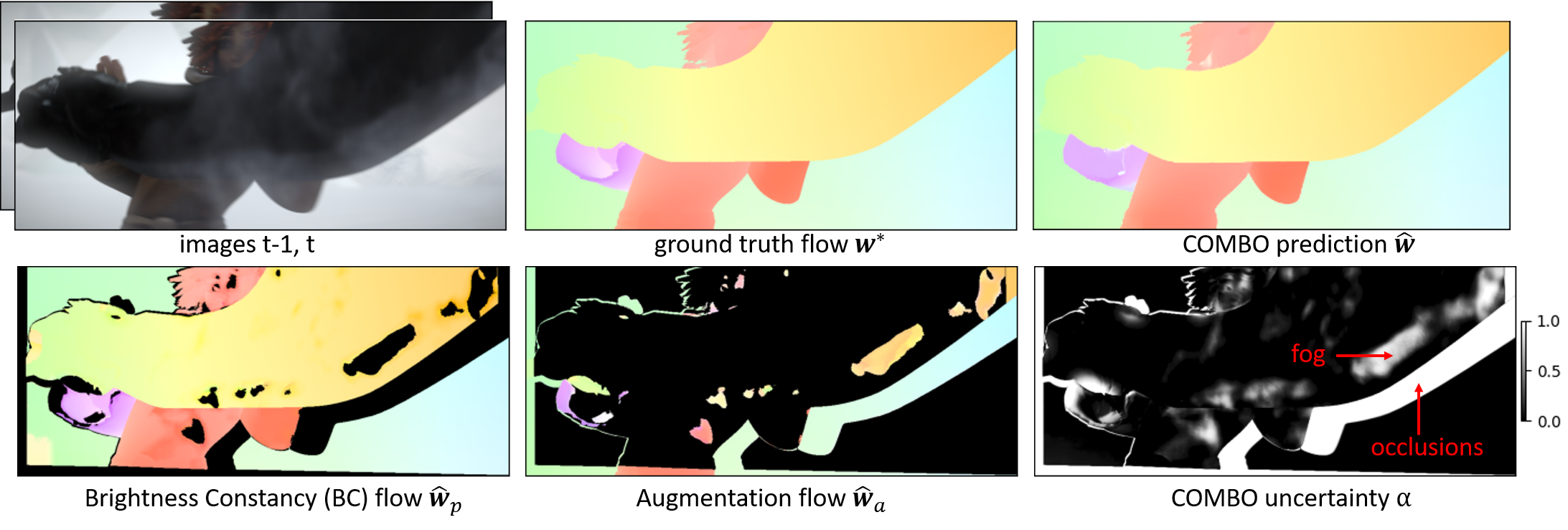
Figure 1: Proposed COMBO model for flow estimation between two images $I_{1}$ and $I_{2}$. We explicitly leverage the brightness constancy (BC) assumption in Eq. (1) for estimating the physical flow prediction $\hat{\mathbf{w}}_{p}$. Since BC is an approximate model violated in several usual situations, COMBO learns an uncertainty map $\hat{\alpha}$ specifying areas where $\hat{\mathbf{w}}_{p}$ is relevant, and an augmentation data-driven flow $\hat{\mathbf{w}}_{a}$ to compensate for the BC violations (in this example, related to fog and occlusions). The final COMBO prediction combining $(\hat{\mathbf{w}}_{a},\hat{\mathbf{w}}_{p},\hat{\alpha})$ is both physically-regularized and accurate.

1 Introduction

Optical flow estimation is a classical problem in computer vision, consisting in computing the per-pixel motion between video frames. This is a core visual task useful in many applications, such as video compression [1], medical imaging [4] or object tracking [11]. Yet, this remains a particularly challenging task for real-world scenes, especially in presence of fast-moving objects, occlusions, changes of illumination or textureless surfaces.

Traditional model-based estimation methods [35, 17] assume that the intensity of pixels is conserved during motion $\mathbf{w}$: $I_{t-1}(\mathbf{x})=I_{t}(\mathbf{x}+\mathbf{w})$, which is known as the brightness constancy (BC) model. Linearizing this constraint for small motion leads to the famous optical flow partial differential equation (PDE) solved by variational methods since the seminal work of Horn and Schunk [17]:

$$\frac{\partial I}{\partial t}(t,\mathbf{x})+\mathbf{w}(t,\mathbf{x})\cdot\nabla I(t,\mathbf{x})=0$$ (1)

However this physical model for optical flow is only a rather coarse approximation of the reality. The BC assumption is violated in many situations: in presence of occlusions, global or local illumination changes, specular reflexions, or complex natural situations such as fog. The correspondence problem is also ambiguous for textureless surfaces. To solve this ill-posed inverse problem, this is necessary to inject prior knowledge about the flow, such as spatial smoothness, sparsity or small total variation.

In contrast to these traditional model-based approaches, deep neural networks have become state-of-the-art for learning optical flow in a pure data-driven fashion [13, 20, 44, 51, 18, 61, 53]. However, since flow labelling on real images is expensive, supervised deep learning methods mostly use complex curriculum training schemes on synthetic datasets to progressively adapt to the complexity of real-world scenes.

More recently, unsupervised deep learning approaches are closer in spirit to traditional approaches [22, 45, 39, 30, 24, 49]. Without ground-truth labels, they rely on a photometric reconstruction loss based on the BC assumption, and additional regularization losses like spatial smoothness. They also use of specific modules, e.g. occlusion detection, to identify images areas where the BC in Eq. (1) is violated.

In this work, we introduce a hybrid model-based machine learning (MB/ML) model dedicated to optical flow estimation, which COMplements Brightness constancy with deep networks for accurate Optical flow prediction (COMBO). As illustrated in Figure 1, COMBO decomposes the estimation process into a physical flow based on the simplified Brightness Constancy (BC) hypothesis and a data-driven augmentation for compensating for the limitations of the physical model. COMBO also simultaneously learns an uncertainty model of the brightness constancy, useful for fusing the two flow branches into an accurate flow estimation. Importantly, the two branches are learned jointly and a principled optimization ensures an optimal cooperation between them.

Our contributions are the following:

• We propose a principled way to regularize supervised flow models with an explicit exploitation of the BC assumption. We introduce with COMBO a meaningful and unique flow decomposition into a physical part optimizing the BC and an augmentation part compensating for its limitations.

• We propose to jointly learn the physical, augmented flows and a uncertainty measure of the BC validity, generalizing occlusion detection approaches or robust photometric losses. It also enables to exploit the model in semi-supervised contexts for non-annotated pixels where we know that the BC assumption is satisfied.

• To learn the COMBO model, we define and compute a fine-grained supervision by decomposing the ground-truth flow into a BC flow, a residual flow and an uncertainty map.

• Experiments (section 4) show that when included into a state-of-the-art supervised network, i.e. RAFT, COMBO can improve performances consistently over datasets and training curriculum steps. COMBO also reaches state-of-the-art performances on several benchmarks, and we show that the semi-supervised scheme can be leveraged to grandly simplify the training curriculum. We also provide detailed ablations and qualitative analyses attesting the benefits of our principled decomposition framework.

2 Related work

Traditional optical flow

Since the seminal works of Lucas-Kanade [35] and Horn-Schunck [17], optical flow estimation is traditionally casted as an optimization problem over the space of motion fields between a pair of images [40, 58, 8]. As mentionned in introduction, the cost function is usually based on the conservation assumption of an image descriptor during motion, i.e. the brightness constancy (BC). Since the number of optical flow variables is twice the number of observations, the search problem is underconstrained. Existing methods typically add spatial smoothness constraints on the flow to regularize the problem, enabling to propagate information from non-ambiguous to ambiguous pixels, e.g. occluded. Since, progress has been made for handling the limitations of the brightness constancy with more robust matching loss, such as the gradient constancy [7], the structural similarity (SSIM), the Charbonnier loss [9], the census loss [39] or involving descriptors learned by deep neural networks [3, 59]. However, these traditional methods are limited for handling large motion and often suffer from a high computational cost.

Deep supervised methods

Deep neural networks have proven effective for directly learning the optical flow end-to-end from a labelled dataset [13, 20, 44, 51, 18, 53, 23]. Although some methods borrow ideas from traditional methods such as cost volume processing [61] and pyramidal coarse-to-fine warping [44], they do not rely anymore on the conservation of an image descriptor. One of the current state-of-the-art architectures is the Recurrent All-Pairs Field Transforms (RAFT) [53]. This model exploits the correlation volume between all pairs of pixels and iteratively refines the flow with a recurrent neural network. Since obtaining ground-truth flow annotations is very expensive, supervised methods mostly train on synthetic datasets. This leads to a non-negligible generalization gap when transferring to real-world datasets. Consequently, complex curriculum learning schemes are needed to progressively adapt the learned optical flow from synthetic data to real scenarios [53, 50].

Deep unsupervised methods

More recently, unsupervised approaches proved to outperform traditional methods even without flow labels [22, 45, 39, 30, 24, 49]. They revisit the brightness constancy assumption by warping the target image with the estimated flow and optimizing a photometric loss. However they still lag behind supervised methods and require additional mechanisms for overcoming the limitations of the BC assumption, e.g. occlusion reasoning [39, 57] or self-supervision [31, 32, 24]. Occlusions were traditionally treated as outliers in a robust estimation setting [7], or estimated with a forward-backward consistency check [2, 39]. More recent approaches jointly learn occlusion maps with convolutional neural networks in a supervised way (i.e. with ground-truth occlusions) [37, 20, 19] or unsupervised way [63, 15, 21]. Nonetheless, most of these methods focus on specific cases of deviations from the brightness constancy assumption, e.g. occlusions or illumination changes. Our approach is more general and learns to compensate for any failure case of this simplified assumption. Besides, we learn from supervised flow data a confidence model of the BC assumption, which enables to learn our model in a semi-supervised setting [26, 60].

Hybrid MB/ML

Combining model-based (MB) and machine learning (ML) models is a long-standing subject [42, 54, 46] that yet remains widely open nowadays. Leveraging physical knowledge enables to design machine learning models that learn from less data, and offer better generalization while conserving physical plausibility. Many ideas were explored, such as imposing soft physical constraints [43, 48, 34, 28, 56] in the training loss function or hard constraints in the network architectures [6, 12, 27, 16, 36, 41]. However, most existing approaches assume a fully-known prior physical model. Very few works have investigated how to exploit incomplete physical models with deep neural networks [33, 38, 47, 29, 62]. Besides, exploiting incomplete physical knowledge in a deep hybrid model has never been explored for optical flow to the best of our knowledge.

3 COMBO model for optical flow

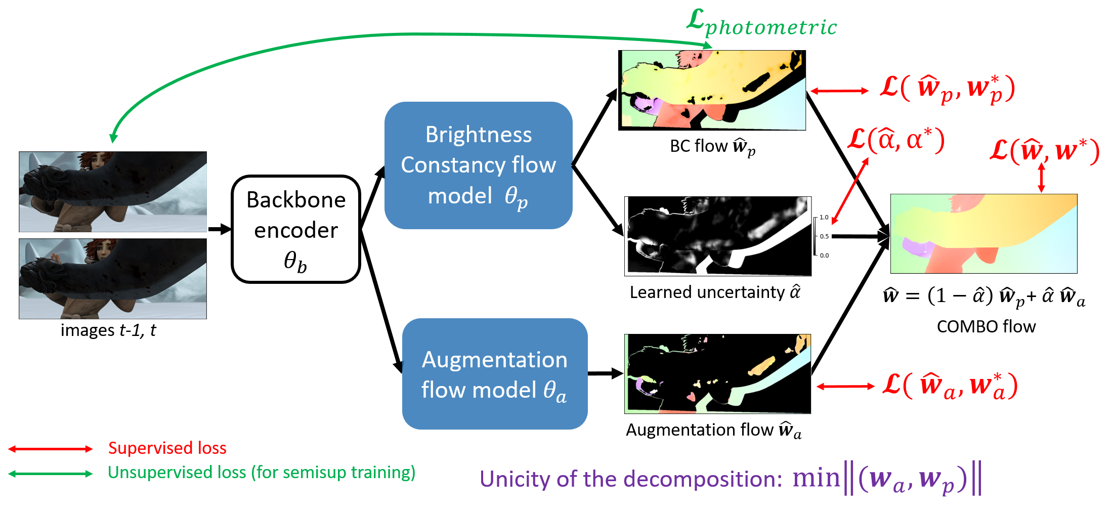
Figure 2: Our proposed COMBO model for optical flow estimation. Given a pair of input frames ($I_{t-1},I_{t}$), COMBO first extract convolutional features. The model is composed of three branches that compute an estimate for the physical flow $\hat{\mathbf{w}}_{p}$, the augmentation flow $\hat{\mathbf{w}}_{a}$ and the uncertainty map $\hat{\alpha}$.

Given a pair of frames $I_{t-1}$ and $I_{t}\in\mathbb{R}^{W\times H\times 3}$, the optical flow task consists in estimating the dense motion field $\mathbf{w}=(u,v)\in\mathbb{R}^{W\times H\times 2}$ that maps each pixel from the source image $I_{t-1}$ to its corresponding relative location in the target image $I_{t}$.

We introduce COMBO, a deep learning model that explicitly exploits the brightness constancy (BC) assumption and learns the complementary information to compensate for the BC modeling errors.

The COMBO model is depicted in Figure 2. The model takes a pair of input frames $(I_{t-1},I_{t})$ and first encodes them into a feature space. From this common representation space, the rationale of COMBO is to decompose the dense flow $\hat{\mathbf{w}}$ using 3 main quantities: a physical term $\hat{\mathbf{w}}_{p}\in\mathbb{R}^{W\times H\times 2}$ fulfilling the BC assumption, an augmentation term $\hat{\mathbf{w}}_{a}\in\mathbb{R}^{W\times H\times 2}$ dedicated to capture the remaining information for accurate flow prediction. For each pixel, our decomposition also involves an uncertainty map $\hat{\alpha}\in[0,1]^{W\times H}$ representing the violation of the BC assumption at each pixel.

In section 3.1, we present our proposed BC augmentation framework, ensuring a unique and meaningful decomposition of $\hat{\mathbf{w}}$ between the physical $\hat{\mathbf{w}}_{p}$, augmented $\hat{\mathbf{w}}_{a}$ and uncertainty $\hat{\alpha}$ terms. From this formulation, we derive in section 3.2 a training scheme to learn the model parameters, including a supervised but also a semi-supervised variant leveraging the learned BC confidence $\hat{\alpha}$.

3.1 BC-augmented flow decomposition

We consider the flow $\mathbf{w}(\mathbf{x})$ representing the displacement of pixel $\mathbf{x}=(x,y)$ from $I_{t-1}(\mathbf{x})$ to $I_{t}(\mathbf{x})$. Let us define the brightness constancy divergence as $\mathcal{L}_{BC}(\mathbf{x},\mathbf{w}):=\ell(I_{t-1}(\mathbf{x})-I_{t}(\mathbf{x}+\mathbf{w}))$ measured with the photometric loss $\ell$ (e.g. the L1 loss). In COMBO, we propose to decompose the ground truth flow $\mathbf{w}^{*}$ between a physical flow $\mathbf{w}_{p}^{*}$, an augmentation flow $\mathbf{w}_{a}^{*}$ and an uncertainty map $\alpha^{*}$:

$$\mathbf{w}^{*}(\mathbf{x})=(1-\alpha^{*}(\mathbf{x}))~{}\mathbf{w}_{p}^{*}(\mathbf{x})+\alpha^{*}(\mathbf{x})~{}\mathbf{w}_{a}^{*}(\mathbf{x}).$$ (2)

Since the decomposition in Eq. (2) is not necessarily unique, we define the COMBO decomposition ($\mathbf{w}_{p}^{*},\mathbf{w}_{a}^{*},\alpha^{*}$) as the solution of the following constrained optimization problem:

$$\underset{\mathbf{w}_{p},\mathbf{w}_{a}}{\min}~{}~{}~{}\left\|(\mathbf{w}_{a},\mathbf{w}_{p})\right\|~{}~{}~{}~{}~{}~{}~{}\text{subject to: ~{}~{}~{}~{}~{}~{}}$$ (3)

$$\begin{cases}(1-\alpha^{*}(\mathbf{x}))~{}\mathbf{w}_{p}(\mathbf{x})+\alpha(\mathbf{x})~{}\mathbf{w}_{a}(\mathbf{x})=\mathbf{w}^{*}(\mathbf{x})\\ (1-\alpha^{*}(\mathbf{x}))~{}|I_{1}(\mathbf{x})-I_{2}(\mathbf{x}+\mathbf{w}_{p}(\mathbf{x}))|=0\\ \alpha^{*}(\mathbf{x})=\sigma\left(|I_{1}(\mathbf{x})-I_{2}(\mathbf{x}+\mathbf{w}^{*}(\mathbf{x}))|\right).\\ \end{cases}$$

Theoretical properties of the decomposition:

Under these constraints, the decomposition problem in Eq. (3) admits a unique solution $(\mathbf{w}_{p}^{*},\mathbf{w}_{a}^{*},\alpha^{*})$ (we detail the proof in supplementary LABEL:sup:proof). The uniqueness in decomposition of a given flow into the three $(\mathbf{w}_{p}^{*},\mathbf{w}_{a}^{*},\alpha^{*})$ components is important since it ensures a well posed problem for learning the different terms.

Beyond its sound mathematical formulation, the decomposition in Eq. (3) is also meaningful. It ensures to properly and explicitly exploit the BC model and to overcome its limitations to represent real data in diverse and complex situations. We detail now each component of this decomposition problem:

Brightness constancy flow $\hat{\mathbf{w}}_{p}(\mathbf{x})$:

We define the brightness constancy flow $\hat{\mathbf{w}}_{p}$ as a minimizer of the BC condition, similarly to traditional and unsupervised methods. The BC is a very useful constraint not fully exploited in deep supervised methods. However, as mentioned in introduction, this BC assumption is often violated in real data, e.g. in case of occlusions, illumination changes, textureless surfaces, etc. When directly minimizing $\mathcal{L}_{BC}(\mathbf{x},\mathbf{w})=\ell(I_{t-1}(\mathbf{x})-I_{t}(\mathbf{x}+\mathbf{w}))$, for a given pixel $\mathbf{x}$ in the source image, there may exist multiple possible matches in the target image satisfying the BC constraint. Therefore, the BC constraint is only applied to $\mathbf{w}_{p}$ in Eq. (3), not to the final flow vector $\mathbf{w}^{*}$, and is weighted by the BC confidence measure ($1-\alpha^{*}(\mathbf{x})$). This is done on purpose, since the BC constraint is not always verified when training a model from ground truth supervision, making this term possibly conflicting with the supervised objective. We verify experimentally that a naive incorporation of the BC loss during training is not effective. In contrast, COMBO exploits an augmented flow to jointly incorporate the BC knowledge with an adaptive compensation for its violation.

BC augmented flow $\hat{\mathbf{w}}_{a}(\mathbf{x})$:

In contrast to traditional and unsupervised methods, we do not leverage prior knowledge on the flow but instead rely on a data-driven augmentation $\hat{\mathbf{w}}_{a}$ to learn how to optimally compensate for the simplified model, as investigated by several recent augmented physical models [33, 55, 38, 47, 29, 62]. To ensure a unique decomposition in Eq. (3), we minimize the norm of the concatenated vector $(\hat{\mathbf{w}}_{a},\hat{\mathbf{w}}_{p})$. The rationale is to compensate with the minimal correction $\|\hat{\mathbf{w}}_{a}\|$ from the brightness constancy assumption. This least-action augmentation also prevents $\hat{\mathbf{w}}_{p}(\mathbf{x})$ from being too large: the BC flow is enforced to be as close as possible to the ground-truth flow $\mathbf{w}^{*}$. Minimizing the norm of $\hat{\mathbf{w}}_{p}$ also prevents degenerate cases with possibly several admissible $\hat{\mathbf{w}}_{p}$ equidistant to $\mathbf{w}^{*}$ (see supplementary LABEL:sup:proof for a discussion).

BC uncertainty $\alpha^{*}(\mathbf{x})$:

We weight the decomposition between $\hat{\mathbf{w}}_{p}$ and $\hat{\mathbf{w}}_{a}$ in Eq. (3) with the uncertainty map $\alpha^{*}(\mathbf{x})=\sigma(\mathcal{L}_{BC}(\mathbf{x},\mathbf{w}^{*}))$ quantifying the per-pixel validity of the BC assumption, where $\sigma$ is a nonlinear function ensuring that the uncertainty values spread over $[0;1]$. When $\alpha^{*}(\mathbf{x})=0$, the BC assumption is verified; in that case, our decomposition reduces to the physical flow $\hat{\mathbf{w}}(\mathbf{x})=\hat{\mathbf{w}}_{p}(\mathbf{x})$ as in traditional methods. On the contrary, when the BC is violated ($\alpha^{*}(\mathbf{x})>0$), the errors of the brightness constancy modelling are compensated by the data-driven model $\hat{\mathbf{w}}_{a}$. This leads to a meaningful decomposition between $\hat{\mathbf{w}}_{p}$ and $\hat{\mathbf{w}}_{a}$.

3.2 Training

In this section, we propose to jointly learn the three quantities $\mathbf{w}_{p}^{*}$, $\mathbf{w}_{a}^{*}$ and $\alpha^{*}$ of the flow decomposition Eq. (2) with a deep neural architecture named COMBO. We introduce a practical learning framework to solve the decomposition problem in Eq. (3) in the supervised and semi-supervised settings. Given a dataset of labelled image pairs $\mathcal{D}_{sup}=\left\{(I_{t-1},I_{t},\mathbf{w}^{*})_{i}\right\}_{i=1}^{N_{sup}}$ and unlabelled image pairs $\mathcal{D}_{unsup}=\left\{(I_{t-1},I_{t})_{i}\right\}_{i=1}^{N_{unsup}}$, the goal is to learn the parameters $\theta=\left\{\theta_{b},\theta_{p},\theta_{a}\right\}$ of the COMBO model depicted in Figure 2, where $\theta_{b}$ are the backbone encoder parameters, $\theta_{p}$ the parameters of the BC flow model, $\theta_{a}$ are the parameters of the augmented flow model.

The general loss for learning the COMBO model is the following:

$$\mathcal{L}(\mathcal{D},\theta)=\lambda_{p}~{}\|\hat{\mathbf{w}}_{p}-\mathbf{w}_{p}^{*}\|_{2}^{2}+\lambda_{a}~{}\|\hat{\mathbf{w}}_{a}-\mathbf{w}_{a}^{*}\|_{2}^{2}+\lambda_{total}~{}\|\hat{\mathbf{w}}-\mathbf{w}^{*}\|_{2}^{2}\\ +\lambda_{photo}~{}\mathcal{L}_{photo}(\mathcal{D},\theta)+\lambda_{w}~{}\|(\hat{\mathbf{w}}_{a},\hat{\mathbf{w}}_{p})\|^{2}+\lambda_{\alpha}~{}\mathcal{L}_{\alpha}(\mathcal{D},\theta),$$ (4)

where $\hat{\mathbf{w}}(\mathbf{x})=(1-\hat{\alpha}(\mathbf{x}))~{}\hat{\mathbf{w}}_{p}(\mathbf{x})+\hat{\alpha}(\mathbf{x})~{}\hat{\mathbf{w}}_{a}(\mathbf{x})$ is the flow predicted by COMBO.

The total loss in Eq. (4) is composed of supervised losses on the final flow $\hat{\mathbf{w}}$, the BC flow $\hat{\mathbf{w}}_{p}$ and the augmentation flow $\hat{\mathbf{w}}_{a}$. In addition to the supervised loss on $\hat{\mathbf{w}}_{p}$, we also use a photometric loss similarly to traditional and unsupervised methods. We use the L1 loss weighted by the certainty measure $(1-\alpha^{*}(\mathbf{x}))$:

$$\mathcal{L}_{photo}(\mathcal{D},\theta)=\sum_{I_{1},I_{2}\in\mathcal{D}}\sum_{\mathbf{x}}\;(1-\alpha^{*}(\mathbf{x}))~{}|I_{1}(\mathbf{x})-I_{2}(\mathbf{x}+\hat{\mathbf{w}}_{p})|_{1}.$$ (5)

With the L1 loss, the physical branch of COMBO directly models the brightness conservation at the pixel level and the learned uncertainty captures the limitations of this hypothesis. Other photometric losses more robust to the brightness constancy limitations could have been chosen, e.g. the Charbonnier [9], SSIM [24] or census loss [39], that would produce a different physical flow. Our augmentation framework can seamlessly adapt to the level of approximation of the BC model at each pixel. Note that the photometric loss is complementary with the supervised loss $\|\hat{\mathbf{w}}_{p}-\mathbf{w}_{p}^{*}\|_{2}^{2}$: a small error on the predicted flow $\hat{\mathbf{w}}_{p}$ results in a small endpoint error (EPE) but can have a large photometric error if $\hat{\mathbf{w}}_{p}$ leads to a large photometric change in the target image.

Finally, we define the uncertainty loss as:

$$\mathcal{L}_{\alpha}(\mathcal{D}_{sup},\theta)=\sum_{I_{1},I_{2}\in\mathcal{D}_{sup}}\sum_{\mathbf{x}}\;\|\hat{\alpha}(\mathbf{x})-\sigma(\mathcal{L}_{BC}(\mathbf{x},\mathbf{w}^{*}))\|_{2}^{2}.$$ (6)

Curriculum learning for the BC uncertainty: In the COMBO decomposition $\hat{\mathbf{w}}(\mathbf{x})=(1-\hat{\alpha}(\mathbf{x}))~{}\hat{\mathbf{w}}_{p}(\mathbf{x})+\hat{\alpha}(\mathbf{x})~{}\hat{\mathbf{w}}_{a}(\mathbf{x})$, a bad estimate of the uncertainty $\alpha$ could be harmful for learning $\hat{\mathbf{w}}_{p}$ and $\hat{\mathbf{w}}_{a}$. Therefore, similarly to the teacher forcing strategy in sequential models, we choose a scheduled sampling strategy [5] where we use the ground truth $\alpha^{*}$ with high probability at the beginning of learning, and decrease progressively this probability towards 0 to rely more and more on the prediction $\hat{\alpha}$ (see Algorithm 1).

3.2.1 Supervised learning:

In the supervised learning setting, we only exploit the supervised set $\mathcal{D}_{sup}$. We minimize the total loss in Eq. (4) by using the fine-grained supervision on $(\mathbf{w}_{p}^{*},\mathbf{w}_{a}^{*},\alpha^{*})$ that we have created (see supplementary LABEL:sup:supervision for examples of tuples $(\mathbf{w}_{p}^{*},\mathbf{w}_{a}^{*},\alpha^{*})$ for each dataset).

3.2.2 Semi-supervised learning:

COMBO can be also favorably used in a semi-supervised training setting, which consists in exploiting the information of non-annotated images in $\mathcal{D}_{unsup}$ in addition to the annotated frames in $\mathcal{D}_{sup}$. This is an important context in practice since labelling flow images is expensive at scale (in general $N_{unsup}\gg N_{sup}$). Leveraging unlabelled data directly on the target dataset is an appealing way for unsupervised domain adaptation.

When learning in semi-supervised mode (see Algorithm 1), we mix in a mini-batch labelled image pairs from $\mathcal{D}_{sup}$ and unlabelled image pairs from $\mathcal{D}_{unsup}$. For labelled images, we again minimize the supervised loss $\mathcal{L}$ defined in Eq. (4). For unlabelled frames, we refine the estimation of $\hat{\mathbf{w}}_{p}$ by exploiting the photometric loss on pixels that are likely to satisfy the BC constraint (measured by the uncertainty map $\alpha$ learned with ground-truth data). We only minimize in that case the photometric loss $\mathcal{L}_{photo}(\mathcal{D}_{unsup},\theta)$, which corresponds to the particular case of Eq. (4) by setting $\lambda_{photo}=1$ and $\lambda_{p}=\lambda_{a}=\lambda_{total}=\lambda_{w}=\lambda_{\alpha}=0$. Importantly, for unlabelled images, we block the gradient flow in the uncertainty branch $\alpha$ since $\alpha$ can only be estimated in supervised mode.

Parameters: $\lambda_{p},\lambda_{a},\lambda_{total},\lambda_{photo},\lambda_{w},\lambda_{\alpha}\geq 0,\tau>0$ ;

for epoch = $1:N_{epochs}$ do

       for each batch $b=(b_{sup},b_{unsup})$ do

            

            If $Rand(0,1)<1-epoch/50$ Then: $~{}~{}~{}~{}\#$ scheduled sampling

            $\hat{\mathbf{w}}(\mathbf{x})=(1-\alpha^{*}(\mathbf{x}))~{}\hat{\mathbf{w}}_{p}(\mathbf{x})+\alpha^{*}(\mathbf{x})~{}\hat{\mathbf{w}}_{a}(\mathbf{x})$

             Else:

             $\hat{\mathbf{w}}(\mathbf{x})=(1-\hat{\alpha}(\mathbf{x}))~{}\hat{\mathbf{w}}_{p}(\mathbf{x})+\hat{\alpha}(\mathbf{x})~{}\hat{\mathbf{w}}_{a}(\mathbf{x})$

             Compute $\mathcal{L}_{sup}=\mathcal{L}(b_{sup},\theta,\lambda_{sup},\lambda_{photo},\lambda_{w},\lambda_{\alpha})$ with Eq. (4)

             Compute $\mathcal{L}_{unsup}=\mathcal{L}_{photo}(b_{unsup},\theta)$

             $\theta_{j+1}=\theta_{j}-\tau~{}\nabla(\mathcal{L}_{sup}+\mathcal{L}_{unsup})\;$

Algorithm 1 COMBO optimization:

Stage Method Chairs Sintel-test-resplit KITTI-test-resplit Clean Final Fl-epe Fl-all C RAFT 0.82 1.11 1.76 10.7 39.7 C COMBO 0.74 1.04 1.58 10.2 39.3 C+T RAFT 1.15 0.82 1.17 5.67 17.9 C+T COMBO 1.09 0.77 0.96 5.46 17.3 C+T+ RAFT 1.23 0.57 0.76 1.79 7.12 S+H+K COMBO 1.16 0.56 0.71 1.75 6.58

Table 1: Performances of COMBO compared to the RAFT model (run with online code). COMBO consistently outperforms RAFT on the three training stages, illustrating the relevance of leveraging the BC physical model and complementing its failure cases.

4 Experiments

We evaluate and compare COMBO to recent state-of-the-art models on the optical flow datasets FlyingChairs [13], MPI Sintel [10] and KITTI-2015 [14], in the supervised and semi-supervised contexts. For model analysis, we perform a train/test resplit of the Sintel and KITTI training datasets, as done by [30]. Our code is available at https://github.com/vincent-leguen/COMBO.

4.1 Experimental setup

We adopt for the backbone encoder and flow network the RAFT architecture [53], which is one of the current state-of-the-art methods for supervised optical flow. The encoder is composed of convolutional layers that extract features from images $I_{t-1}$ and $I_{t}$ at resolution $1/8$. Then visual similarity is modelled by constructing a 4D correlation volume that computes matching costs for all possible displacements. The optical flow branch is a gated recurrent unit (GRU) that progressively refines the flow from an initial estimate, with lookups on the correlation volume. The final flow is the sum of residual refinements from the GRU, upsampled at full resolution.

In the COMBO model, the encoder and correlation volume are shared, and each branch has its own GRU initialized from zero. The uncertainty branch is simply adapted to provide a unique output channel. We give details on the network architectures and hyperparameters in supplementary LABEL:sup:implem. The code of COMBO will be released if accepted. Note that our method is agnostic to the optical flow backbone. Any other deep architecture than RAFT could be used for computing the physical, augmentation flow and the uncertainty map.

4.2 Supervised state-of-the-art comparison

Following the supervised learning curriculum of prior works [63, 52, 53, 23], we pretrain our models successively on the synthetic datasets FlyingChairs [13] and FlyingThings3D [37]. We then finetune on Sintel [10] by combining data from Sintel, KITTI-2015 and HD1K [25]. We finally finetune on KITTI-2015 with only data from KITTI.

Stage Method Chairs Sintel (train) KITTI-15 (train) Clean Final Fl-epe Fl-all C RAFT [53] 0.82 2.26 4.52 10.67 39.72 C GMA [23] 0.79 2.32 4.10 10.32 36.91 C COMBO 0.74 2.19 4.37 10.19 39.02 C+T LiteFlowNet [20] - 2.48 4.04 10.39 28.5 C+T PWC-Net [51] - 2.55 3.93 10.35 33.7 C+T VCN [61] - 2.21 3.68 8.36 25.1 C+T MaskFlowNet [63] - 2.25 3.61 - 23.1 C+T RAFT [53] 1.15 1.43 2.71 5.01 17.5 C+T GMA [23] 1.19 1.31 2.73 4.69 17.1 C+T COMBO 1.09 1.31 2.58 4.69 16.5

Table 2: State-of-the-art performance comparison on FlyingChairs, Sintel-train and KITTI-train, when learning on FlyingChairs (C) and FlyingChairs+FlyingThings (C+T). Scores are reported from corresponding papers.

In Table 1, we compare the endpoint error (EPE) of COMBO with RAFT [53], by running the code from the authors. Since we rely on a RAFT architecture, the results in Table 1 directly evaluate the impact of the proposed augmented model and learning scheme. We see that COMBO consistently outperforms RAFT on FlyingChairs, Sintel-test-resplit and KITTI-test-resplit from all stages of the curriculum. This confirms the relevance of leveraging the BC constraint for regularizing supervised models, and the use of the augmentation for compensating its violations.

In Table 2, we compare COMBO to competitive supervised optical flow baselines, from the stages FlyingChairs (C) and FlyingChairs+FlyingThings (C+T). When generalizing to Sintel-train and KITTI-train, COMBO outperforms RAFT [53] in all cases, and is superior or equivalent to the recent GMA model [23] in 6/8 cases. Note also that COMBO outperforms all other methods on FlyingChairs.

4.3 Semi-supervised results

model	mode	checkpoint	KITTI (test-resplit)
			F1-epe	F1-all
RAFT [53]	sup	C	2.28	7.60
COMBO	sup	C	2.19	7.30
COMBO	semisup	C	1.75	6.88
RAFT [53]	sup	S	1.79	7.12
COMBO	sup	S	1.75	6.58
COMBO	semisup	S	1.74	6.58

Table 3: Comparison with RAFT on KITTI-test-resplit from the FlyingChairs (C) and Sintel (S) checkpoints, with supervised and semisup training on KITTI. We see that COMBO in semisup from Chairs is almost equivalent to COMBO from Sintel, showing that the training curriculum can be drastically reduced.

We analyze the performances of COMBO in a semi-supervised learning setting in Table 3. We evaluate the different models on KITTI test-resplit, using for training the annotated images of KITTI train-resplit (sup) and the additional unlabelled images of KITTI (semisup). When training on KITTI from the earliest stage of the curriculum (FlyingChairs), we can see that COMBO-semisup (Fl-epe=1.75) largely improves over RAFT-sup (2.28) and COMBO-sup (2.19). It confirms that leveraging the vast amount of unlabelled frames is crucial for adapting the model to a target dataset from an early checkpoint. Interestingly, the semisup training from Chairs is almost equivalent to the COMBO model trained from the Sintel checkpoint (1.74). It shows that COMBO trained in a semisup context enables to greatly simplify the training curriculum to reach similar performances. This feature of COMBO is of crucial interest in many domains for transferring models to target datasets from a single synthetic training stage.

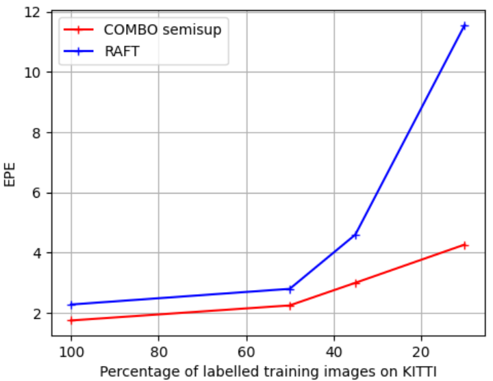
Figure 3: Performances on KITTI-resplit trained from the Chairs, w.r.t. the number of labelled frames.

To further analyze the semi-supervised learning ability of COMBO, we progressively reduce the number of training images on KITTI-resplit and compare the performances of RAFT and COMBO-semisup trained from the FlyingChairs checkpoint. In Figure 3, we observe that RAFT degrades much more sharply than COMBO with fewer training images, and the difference in EPE becomes very large with 10% of training images (EPE=11.6 for RAFT v.s. 4.4 for COMBO). It highlights the crucial ability of COMBO to leverage the BC assumption on unlabelled frames.

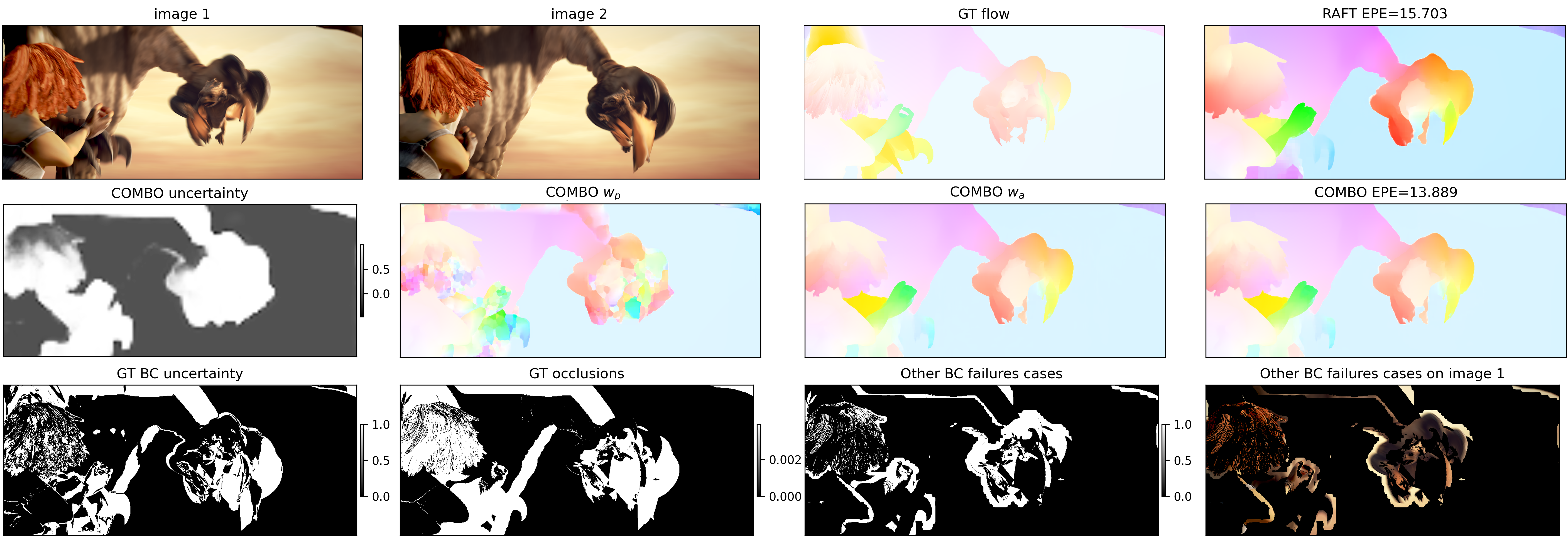
Figure 4: Qualitative prediction results on MPI Sintel. We observe that in zones of high uncertainty of the BC, the physical flow $\hat{\mathbf{w}}_{p}$ is ill-defined; the augmentation flow $\hat{\mathbf{w}}_{a}$ successfully complements it for accurate flow estimation. We also show that the uncertainty learned by COMBO is consistent with the GT BC uncertainty, and that it detects other cases of violation of the BC different from occlusions.

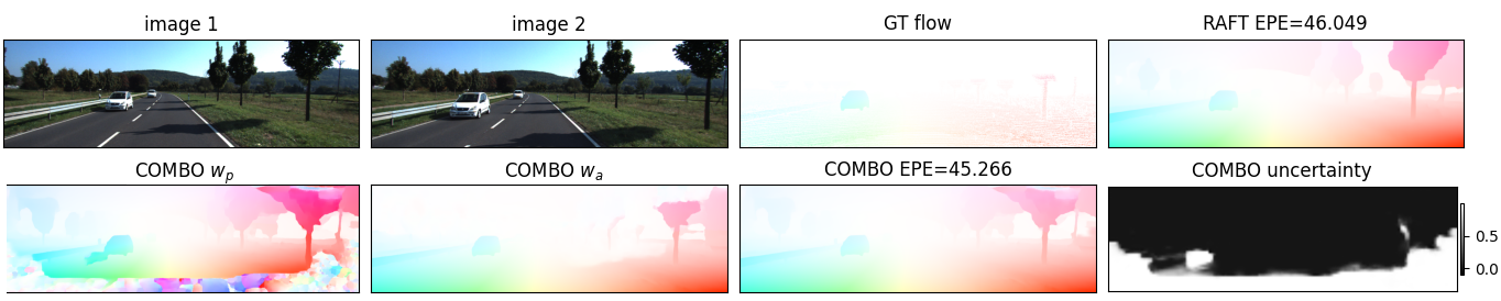
Figure 5: Qualitative prediction results on KITTI 2015. We see that at the bottom of the image where the road becomes occluded, the physical flow $\hat{\mathbf{w}}_{p}$ is ill-defined and is complements by $\hat{\mathbf{w}}_{a}$ for accurate prediction.

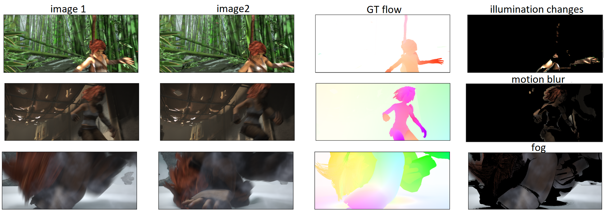
Figure 6: Failure cases of the brightness constancy detected by COMBO different from occlusions. The last column corresponds to image 1 masked by the map of thresholded uncertainty $\hat{\alpha}$ deprived of the ground-truth occlusions. From top to bottom, COMBO captures: illumination change, motion blur and fog.

4.4 Ablation study

We perform in Table 4 an ablation study on FlyingChairs to analyze the behaviour of the COMBO model. We first show that two RAFT branches trained with different seeds and mixed 50:50 improve over RAFT but is largely inferior to COMBO, show that the performances of COMBO do not simply come from an augmentation of the parameters or an ensembling effect. Then, we see that a single RAFT branch with the photometric loss $\mathcal{L}_{photo}$ in Eq. (5) (epe=0.794) is far inferior to COMBO (0.743). This is because the BC regularization helps in improving generalization in regions where the BC assumption is fulfilled, but is detrimental in regions where the BC assumption does not hold. In contrast, COMBO can leverage the BC assumption and complement it in an adaptive manner when it is violated, overcoming the conflict issues between the two terms.

Moreover, the linear decomposition $\hat{\mathbf{w}}=\hat{\mathbf{w}}_{p}+\hat{\mathbf{w}}_{a}$ without the uncertainty branch, i.e. we set $\alpha(\mathbf{x})=1/2$ everywhere, is clearly inferior to COMBO. It shows the crucial necessity to account for the uncertainty of the BC. Finally, when we remove the minimization of $\|(\hat{\mathbf{w}}_{a},\hat{\mathbf{w}}_{p})\|$ from COMBO (then the decomposition is not unique anymore), the performances also decrease, highlighting the superiority of the well-posed and unique decomposition of COMBO.

We then report in Table 5 the performances of the individual $\hat{\mathbf{w}}_{p}$ (resp. $\hat{\mathbf{w}}_{a}$) branches weighted by the certainty of the BC (resp. uncertainty). For example, we compute $EPE_{weighted}(\hat{\mathbf{w}}_{p},\mathbf{w}^{*})=\sum_{\mathbf{x}}(1-\alpha^{*}(\mathbf{x}))\|\hat{\mathbf{w}}_{p}(\mathbf{x})-\mathbf{w}^{*}(\mathbf{x})\|_{2}$. We see that both $\hat{\mathbf{w}}_{p}$ and $\hat{\mathbf{w}}_{a}$ are superior to RAFT on areas where they apply. In particular the performance gap compared to RAFT widens on areas with high BC uncertainty (EPE= 2.20 v.s. 0.52), showing the benefits of the COMBO decomposition to greatly improve the estimation on challenging zones.

Method	EPE (FlyingChairs)
RAFT [53]	0.818
2 RAFT branches mixed equally	0.800
RAFT + BC photometric loss	0.794
COMBO $\hat{\mathbf{w}}_{p}+\hat{\mathbf{w}}_{a}$ (no weighting by uncertainty)	0.769
COMBO without $\min\|(\hat{\mathbf{w}}_{a},\hat{\mathbf{w}}_{p})\|$	0.752
COMBO	0.743

Table 4: Ablation study on FlyingChairs, showing the benefits of the meaningful and principled decomposition of COMBO, compared to the backbone RAFT.

Method	EPE weighted (FlyingChairs)
RAFT on BC certain zones	0.48
COMBO $\hat{\mathbf{w}}_{p}$ on certain zones	0.30
RAFT on BC uncertain zones	2.29
COMBO $\hat{\mathbf{w}}_{a}$ on uncertain zones	0.52

Table 5: Performances of the individual BC $\hat{\mathbf{w}}_{p}$ and residual $\hat{\mathbf{w}}_{a}$ flow branches on areas with high BC confidence (resp. high BC uncertainty).

4.5 COMBO analysis

We provide qualitative flow predictions of the COMBO model for Sintel-test-resplit in Figure 4 and KITTI-test-resplit in Figure 5. In uncertain zones ($\hat{\alpha}\approx 1$, for example in the occluded region of the bird in Figure 4 or at the bottom of Figure 5), we can see that $\hat{\mathbf{w}}_{p}$ gives incoherent results, as expected. In that case, the flow is efficiently complemented by $\hat{\mathbf{w}}_{a}$ to produce the COMBO flow.

Occlusion detection: To analyze the ability of COMBO to detect occlusions, we represent in supplementary LABEL:sup:combo-analysis the precision-recall curve of the COMBO uncertainty detector with respect to the ground-truth occlusion masks (which are known for Sintel). COMBO obtains an Average Precision (AP) of 59%, which is a lower bound of the true AP of COMBO for occlusions (since COMBO also captures other failure cases than occlusions). This means that COMBO is able to efficiently detect occlusions without any ground-truth occlusion supervision, compared to the random classifier which reaches 7% (ratio of occluded pixels).

Detection of other failure cases of the BC: In the third line of Figure 4, we show the ground-truth (GT) BC uncertainty mask (defined as $\mathcal{L}_{BC}>\epsilon$, $\epsilon=0.01$ in Figure 4) and the ground-truth occlusions of Sintel. We observe that the COMBO uncertainty globally aligns with the GT BC uncertainty, and covers a larger area than the GT occlusions. To investigate this, we display the thresholded uncertainty mask $\alpha$ deprived of the GT occlusions: it shows that COMBO can capture other failure cases of the BC different than occlusions. Applying this mask on image 1 (bottom right of Figure 4) shows that this corresponds to illumination changes for this example.

We further analyze the other failure cases of the BC in Figure 6. We can see that COMBO can detect other cases of violation of the BC, without any supervision masks on these cases. The top row of Figure 6 shows that the uncertainty $\alpha$ detects the illumination change on the arm of the woman. On the middle row, the uncertainty concentrates on the woman running, which causes motion blur. The bottom row shows a BC uncertainty on a large part of the image, caused by the presence of fog. We provide additional visualizations in supplementary LABEL:sup:visus.

5 Conclusion

We have introduced COMBO, a new physically-constrained architecture for optical flow estimation that explicitly exploits the simplified brightness constancy constraint. COMBO learns the uncertainty of the BC and how to complement it with a data-driven network. COMBO reaches state-of-the-art results on several benchmarks, and is able to greatly simplify the training curriculum with a semi-supervised learning scheme. An appealing perspective would be to investigate the application of augmented physical models to multi-frame optical flow estimation.

References

- [1] Agustsson, E., Minnen, D., Johnston, N., Balle, J., Hwang, S.J., Toderici, G.: Scale-space flow for end-to-end optimized video compression. In: Proceedings of the IEEE/CVF Conference on Computer Vision and Pattern Recognition. pp. 8503–8512 (2020)
- [2] Alvarez, L., Deriche, R., Papadopoulo, T., Sánchez, J.: Symmetrical dense optical flow estimation with occlusions detection. International Journal of Computer Vision 75(3), 371–385 (2007)
- [3] Bailer, C., Varanasi, K., Stricker, D.: Cnn-based patch matching for optical flow with thresholded hinge embedding loss. In: Proceedings of the IEEE Conference on Computer Vision and Pattern Recognition. pp. 3250–3259 (2017)
- [4] Balakrishnan, G., Zhao, A., Sabuncu, M.R., Guttag, J., Dalca, A.V.: An unsupervised learning model for deformable medical image registration. In: Proceedings of the IEEE conference on computer vision and pattern recognition. pp. 9252–9260 (2018)
- [5] Bengio, S., Vinyals, O., Jaitly, N., Shazeer, N.: Scheduled sampling for sequence prediction with recurrent neural networks. Advances in neural information processing systems 28 (2015)
- [6] de Bezenac, E., Pajot, A., Gallinari, P.: Deep learning for physical processes: Incorporating prior scientific knowledge. ICLR (2018)
- [7] Brox, T., Bruhn, A., Papenberg, N., Weickert, J.: High accuracy optical flow estimation based on a theory for warping. In: European conference on computer vision. pp. 25–36. Springer (2004)
- [8] Brox, T., Malik, J.: Large displacement optical flow: descriptor matching in variational motion estimation. IEEE transactions on pattern analysis and machine intelligence 33(3), 500–513 (2010)
- [9] Bruhn, A., Weickert, J., Schnörr, C.: Lucas/kanade meets horn/schunck: Combining local and global optic flow methods. International journal of computer vision 61(3), 211–231 (2005)
- [10] Butler, D.J., Wulff, J., Stanley, G.B., Black, M.J.: A naturalistic open source movie for optical flow evaluation. In: European conference on computer vision. pp. 611–625. Springer (2012)
- [11] Corpetti, T., Mémin, É., Pérez, P.: Dense estimation of fluid flows. IEEE Transactions on pattern analysis and machine intelligence 24(3), 365–380 (2002)
- [12] Daw, A., Thomas, R.Q., Carey, C.C., Read, J.S., Appling, A.P., Karpatne, A.: Physics-guided architecture (pga) of neural networks for quantifying uncertainty in lake temperature modeling. In: Proceedings of the 2020 siam international conference on data mining. pp. 532–540. SIAM (2020)
- [13] Dosovitskiy, A., Fischer, P., Ilg, E., Hausser, P., Hazirbas, C., Golkov, V., Van Der Smagt, P., Cremers, D., Brox, T.: Flownet: Learning optical flow with convolutional networks. In: Proceedings of the IEEE international conference on computer vision (ICCV). pp. 2758–2766 (2015)
- [14] Geiger, A., Lenz, P., Stiller, C., Urtasun, R.: Vision meets robotics: The kitti dataset. The International Journal of Robotics Research 32(11), 1231–1237 (2013)
- [15] Godet, P., Boulch, A., Plyer, A., Le Besnerais, G.: Starflow: A spatiotemporal recurrent cell for lightweight multi-frame optical flow estimation. In: 2020 25th International Conference on Pattern Recognition (ICPR). pp. 2462–2469. IEEE (2021)
- [16] Greydanus, S., Dzamba, M., Yosinski, J.: Hamiltonian neural networks. In: Advances in Neural Information Processing Systems (NeurIPS). pp. 15353–15363 (2019)
- [17] Horn, B.K., Schunck, B.G.: Determining optical flow. Artificial intelligence 17(1-3), 185–203 (1981)
- [18] Hui, T.W., Tang, X., Loy, C.C.: Liteflownet: A lightweight convolutional neural network for optical flow estimation. In: Proceedings of the IEEE conference on computer vision and pattern recognition (CVPR). pp. 8981–8989 (2018)
- [19] Hur, J., Roth, S.: Iterative residual refinement for joint optical flow and occlusion estimation. In: Proceedings of the IEEE/CVF Conference on Computer Vision and Pattern Recognition. pp. 5754–5763 (2019)
- [20] Ilg, E., Mayer, N., Saikia, T., Keuper, M., Dosovitskiy, A., Brox, T.: Flownet 2.0: Evolution of optical flow estimation with deep networks. In: Proceedings of the IEEE conference on computer vision and pattern recognition. pp. 2462–2470 (2017)
- [21] Janai, J., Guney, F., Ranjan, A., Black, M., Geiger, A.: Unsupervised learning of multi-frame optical flow with occlusions. In: Proceedings of the European Conference on Computer Vision (ECCV). pp. 690–706 (2018)
- [22] Jason, J.Y., Harley, A.W., Derpanis, K.G.: Back to basics: Unsupervised learning of optical flow via brightness constancy and motion smoothness. In: European Conference on Computer Vision. pp. 3–10. Springer (2016)
- [23] Jiang, S., Campbell, D., Lu, Y., Li, H., Hartley, R.: Learning to estimate hidden motions with global motion aggregation. CVPR (2021)
- [24] Jonschkowski, R., Stone, A., Barron, J.T., Gordon, A., Konolige, K., Angelova, A.: What matters in unsupervised optical flow. In: Computer Vision–ECCV 2020: 16th European Conference, Glasgow, UK, August 23–28, 2020, Proceedings, Part II 16. pp. 557–572. Springer (2020)
- [25] Kondermann, D., Nair, R., Honauer, K., Krispin, K., Andrulis, J., Brock, A., Gussefeld, B., Rahimimoghaddam, M., Hofmann, S., Brenner, C., et al.: The hci benchmark suite: Stereo and flow ground truth with uncertainties for urban autonomous driving. In: Proceedings of the IEEE Conference on Computer Vision and Pattern Recognition Workshops. pp. 19–28 (2016)
- [26] Lai, W.S., Huang, J.B., Yang, M.H.: Semi-supervised learning for optical flow with generative adversarial networks. In: Proceedings of the 31st International Conference on Neural Information Processing Systems. pp. 353–363 (2017)
- [27] Le Guen, V., Thome, N.: Disentangling physical dynamics from unknown factors for unsupervised video prediction. In: CVPR (2020)
- [28] Li, Z., Kovachki, N., Azizzadenesheli, K., Liu, B., Bhattacharya, K., Stuart, A., Anandkumar, A.: Fourier neural operator for parametric partial differential equations. arXiv preprint arXiv:2010.08895 (2020)
- [29] Linial, O., Eytan, D., Shalit, U.: Generative ODE modeling with known unknowns. ICLR 2020 Deep Differential Equations Workshop (2020)
- [30] Liu, L., Zhang, J., He, R., Liu, Y., Wang, Y., Tai, Y., Luo, D., Wang, C., Li, J., Huang, F.: Learning by analogy: Reliable supervision from transformations for unsupervised optical flow estimation. In: Proceedings of the IEEE/CVF Conference on Computer Vision and Pattern Recognition. pp. 6489–6498 (2020)
- [31] Liu, P., King, I., Lyu, M.R., Xu, J.: Ddflow: Learning optical flow with unlabeled data distillation. In: Proceedings of the AAAI Conference on Artificial Intelligence. vol. 33, pp. 8770–8777 (2019)
- [32] Liu, P., Lyu, M., King, I., Xu, J.: Selflow: Self-supervised learning of optical flow. In: Proceedings of the IEEE/CVF Conference on Computer Vision and Pattern Recognition. pp. 4571–4580 (2019)
- [33] Long, Y., She, X., Mukhopadhyay, S.: Hybridnet: integrating model-based and data-driven learning to predict evolution of dynamical systems. Conference on Robot Learning (CoRL) (2018)
- [34] Lu, L., Jin, P., Karniadakis, G.E.: Deeponet: Learning nonlinear operators for identifying differential equations based on the universal approximation theorem of operators. arXiv preprint arXiv:1910.03193 (2019)
- [35] Lucas, B.D., Kanade, T., et al.: An iterative image registration technique with an application to stereo vision. Vancouver, British Columbia (1981)
- [36] Lutter, M., Ritter, C., Peters, J.: Deep lagrangian networks: Using physics as model prior for deep learning. arXiv preprint arXiv:1907.04490 (2019)
- [37] Mayer, N., Ilg, E., Hausser, P., Fischer, P., Cremers, D., Dosovitskiy, A., Brox, T.: A large dataset to train convolutional networks for disparity, optical flow, and scene flow estimation. In: Proceedings of the IEEE conference on computer vision and pattern recognition. pp. 4040–4048 (2016)
- [38] Mehta, V., Char, I., Neiswanger, W., Chung, Y., Schneider, J.: Neural dynamical systems. ICLR 2020 Deep Differential Equations Workshop (2020)
- [39] Meister, S., Hur, J., Roth, S.: Unflow: Unsupervised learning of optical flow with a bidirectional census loss. In: Thirty-Second AAAI Conference on Artificial Intelligence (2018)
- [40] Mémin, E., Pérez, P.: Dense estimation and object-based segmentation of the optical flow with robust techniques. IEEE Transactions on Image Processing 7(5), 703–719 (1998)
- [41] Mohan, A.T., Lubbers, N., Livescu, D., Chertkov, M.: Embedding hard physical constraints in neural network coarse-graining of 3d turbulence. arXiv preprint arXiv:2002.00021 (2020)
- [42] Psichogios, D.C., Ungar, L.H.: A hybrid neural network-first principles approach to process modeling. AIChE Journal 38(10), 1499–1511 (1992)
- [43] Raissi, M.: Deep hidden physics models: Deep learning of nonlinear partial differential equations. The Journal of Machine Learning Research 19(1), 932–955 (2018)
- [44] Ranjan, A., Black, M.J.: Optical flow estimation using a spatial pyramid network. In: Proceedings of the IEEE conference on computer vision and pattern recognition (CVPR). pp. 4161–4170 (2017)
- [45] Ren, Z., Yan, J., Ni, B., Liu, B., Yang, X., Zha, H.: Unsupervised deep learning for optical flow estimation. In: Thirty-First AAAI Conference on Artificial Intelligence (2017)
- [46] Rico-Martinez, R., Anderson, J., Kevrekidis, I.: Continuous-time nonlinear signal processing: a neural network based approach for gray box identification. In: Proceedings of IEEE Workshop on Neural Networks for Signal Processing. pp. 596–605. IEEE (1994)
- [47] Saha, P., Dash, S., Mukhopadhyay, S.: PhICNet: Physics-incorporated convolutional recurrent neural networks for modeling dynamical systems. arXiv preprint arXiv:2004.06243 (2020)
- [48] Sirignano, J., Spiliopoulos, K.: Dgm: A deep learning algorithm for solving partial differential equations. Journal of computational physics 375, 1339–1364 (2018)
- [49] Stone, A., Maurer, D., Ayvaci, A., Angelova, A., Jonschkowski, R.: Smurf: Self-teaching multi-frame unsupervised raft with full-image warping. In: Proceedings of the IEEE/CVF Conference on Computer Vision and Pattern Recognition. pp. 3887–3896 (2021)
- [50] Sun, D., Vlasic, D., Herrmann, C., Jampani, V., Krainin, M., Chang, H., Zabih, R., Freeman, W.T., Liu, C.: Autoflow: Learning a better training set for optical flow. In: Proceedings of the IEEE/CVF Conference on Computer Vision and Pattern Recognition. pp. 10093–10102 (2021)
- [51] Sun, D., Yang, X., Liu, M.Y., Kautz, J.: Pwc-net: Cnns for optical flow using pyramid, warping, and cost volume. In: Proceedings of the IEEE conference on computer vision and pattern recognition (CVPR). pp. 8934–8943 (2018)
- [52] Sun, D., Yang, X., Liu, M.Y., Kautz, J.: Models matter, so does training: An empirical study of cnns for optical flow estimation. IEEE transactions on pattern analysis and machine intelligence 42(6), 1408–1423 (2019)
- [53] Teed, Z., Deng, J.: RAFT: recurrent all-pairs field transforms for optical flow. In: European Conference on Computer Vision (ECCV) (2020)
- [54] Thompson, M.L., Kramer, M.A.: Modeling chemical processes using prior knowledge and neural networks. AIChE Journal 40(8), 1328–1340 (1994)
- [55] Wang, Q., Li, F., Tang, Y., Xu, Y.: Integrating model-driven and data-driven methods for power system frequency stability assessment and control. IEEE Transactions on Power Systems 34(6), 4557–4568 (2019)
- [56] Wang, S., Wang, H., Perdikaris, P.: Learning the solution operator of parametric partial differential equations with physics-informed deeponets. arXiv preprint arXiv:2103.10974 (2021)
- [57] Wang, Y., Yang, Y., Yang, Z., Zhao, L., Wang, P., Xu, W.: Occlusion aware unsupervised learning of optical flow. In: Proceedings of the IEEE Conference on Computer Vision and Pattern Recognition. pp. 4884–4893 (2018)
- [58] Wedel, A., Cremers, D., Pock, T., Bischof, H.: Structure-and motion-adaptive regularization for high accuracy optic flow. In: 2009 IEEE 12th International Conference on Computer Vision. pp. 1663–1668. IEEE (2009)
- [59] Xu, J., Ranftl, R., Koltun, V.: Accurate optical flow via direct cost volume processing. In: Proceedings of the IEEE Conference on Computer Vision and Pattern Recognition. pp. 1289–1297 (2017)
- [60] Yan, W., Sharma, A., Tan, R.T.: Optical flow in dense foggy scenes using semi-supervised learning. In: Proceedings of the IEEE/CVF Conference on Computer Vision and Pattern Recognition. pp. 13259–13268 (2020)
- [61] Yang, G., Ramanan, D.: Volumetric correspondence networks for optical flow. Advances in neural information processing systems 32, 794–805 (2019)
- [62] Yin, Y., Le Guen, V., Dona, J., Ayed, I., de Bézenac, E., Thome, N., Gallinari, P.: Augmenting physical models with deep networks for complex dynamics forecasting. In: Ninth International Conference on Learning Representations ICLR 2021 (2021)
- [63] Zhao, S., Sheng, Y., Dong, Y., Chang, E.I., Xu, Y., et al.: Maskflownet: Asymmetric feature matching with learnable occlusion mask. In: Proceedings of the IEEE/CVF Conference on Computer Vision and Pattern Recognition. pp. 6278–6287 (2020)