Flares and rotation of M dwarfs
with habitable zones accessible to TESS planet detections

Context. More than 4000 exoplanets have been discovered to date, providing the search for a place capable of hosting life with a large number of targets. With the Transiting Exoplanet Survey Satellite (TESS) having completed its primary mission in July 2020, the number of planets confirmed by follow-up observations is growing further. Crucial for planetary habitability is not only a suitable distance of the planet to its host star, but also the star’s properties. Stellar magnetic activity, and especially flare events, expose planets to a high photon flux and potentially erode their atmospheres. Here especially the poorly constrained high-energy UV and X-ray domain is relevant.
Aims. We characterize the magnetic activity of M dwarfs to provide the planet community with information on the energy input from the star; in particular, in addition to the frequency of optical flares directly observed with TESS, we aim at estimating the corresponding X-ray flare frequencies, making use of the small pool of known events observed simultaneously in both wavebands.
Method. We identified $112$ M dwarfs with a TESS magnitude $\leq 11.5$ for which TESS can probe the full habitable zone for transits. These $112$ stars have $1276$ two-minute cadence TESS LCs from the primary mission, which we searched for rotational modulation and flares. We study the link between rotation and flares and between flare properties, for example the flare amplitude-duration relation and cumulative flare energy frequency distributions (FFDs). Assuming that each optical flare is associated with a flare in the X-ray band, and making use of published simultaneous Kepler/K2 and XMM-Newton flare studies, we estimate the X-ray energy released by our detected TESS flare events. Our calibration also involves the relation between flare energies in the TESS and K2 bands.
Results. We detected more than $2500$ optical flare events on a fraction of about $32\%$ of our targets and found reliable rotation periods only for $12$ stars, which is a fraction of about $11$ %. For these $12$ targets, we present cumulative FFDs and FFD power law fits. We construct FFDs in the X-ray band by calibrating optical flare energies to the X-rays. In the absence of directly observed X-ray FFDs for main-sequence stars, our predictions can serve for estimates of the high-energy input to the planet of a typical fast-rotating early- or mid-M dwarf.

1 Introduction

With the advent of the Kepler mission (Borucki et al., 2010), M dwarfs are now known to be the most prolific planet hosts thanks to the abundance of such low-mass stars in our Galaxy and their favorable radius contrast for transit surveys. Moreover, the close-in habitable zones (HZs) of M dwarfs imply a high probability of finding planets that potentially host life. From Kepler detection statistics on average each M dwarf was estimated to be orbited by more than two small planets, and at least one in ten M dwarfs is expected to harbor a planet in its HZ (Dressing & Charbonneau, 2015).

In the wake of exoplanet surveys the magnetic activity of the host stars has gained enormous interest. In particular the high-energy X-ray and ultraviolet (XUV) emission from the outer atmospheres of late-type stars and the notorious variability of their radiation are key elements to be considered in studies of the evolution of planet atmospheres. Various types of models for atmospheric mass loss in strongly irradiated planets have been developed (e.g., Tian et al. 2008a, Tian et al. 2008b, Johnstone et al. 2015, Tu et al. 2015). Even if the planet atmospheres are not removed by the stellar irradiation, their chemistry may be affected; for example Tilley et al. (2019) have calculated that frequent flaring may destruct ozone layers.

Having boosted the interest in understanding the host star’s magnetic phenomena because of their relevance for exoplanets, the same instruments that detect planets through their transits serve as a basis to investigate the host star’s magnetic activity. In addition to Kepler and its successor, the K2 mission (Howell et al., 2014), the Transiting Exoplanet Survey Satellite (TESS, Ricker et al. 2015) plays a major role in this field. At the optical wavelengths where these satellites operate, magnetic activity is manifest most prominently in rotational modulation due to starspots and stochastic brightness outbursts called flares. Light curves (LCs) obtained with these missions present a number of activity diagnostics, including the period and amplitude of starspot modulations, and the energy and frequency of optical flare events (e.g., Davenport et al. 2014, Hawley et al. 2014, Stelzer et al. 2016, Ilin et al. 2019, Raetz et al. 2020, Günther et al. 2020, Medina et al. 2020). In contrast, no telescopes exist that are dedicated to the study of the UV and X-ray counterparts of these events, which are more influential for planet evolution. Since the variability of the stellar high-energy emission is difficult to constrain from observations, we pursue here an indirect approach, calibrating the frequency of X-ray flares on M dwarfs from the observations of optical flares observed with TESS.

TESS is a NASA satellite launched in April 2018, and it completed its (nearly) all-sky survey primary mission in July 2020. It continues to operate and is currently conducting a second all-sky survey. For the primary mission, 2-minute cadence LCs and target pixel files (TPFs) are available for about $200000$ preselected targets. Target pixel files typically contain $11\times 11$ CCD pixels with the target located in the center of the image. Targets for 2-minute cadence observations have been preselected based on the TESS Input Catalog (TIC; Stassun et al. 2018). The TIC contains astronomical and physical parameters for about 470 million point sources and two million extended sources. Further, full frame images are available in 30-minute cadence for the primary mission, containing the flux of all pixels of a single CCD.

Our work is based on a sample of $112$ M dwarfs observed in 2-minute cadence with TESS and with their entire HZs accessible to the detection of planet transits with TESS. We explain our sample selection and the calculation of the stellar parameters in Sect. 2. Sect. 3 describes our LC analysis procedure to search for rotation periods and flares. We give the results of this analysis in Sect. 4, including relations between flare rate and spectral type (SpT), FFDs and a discussion of detection biases. Confirmed planet host stars and TESS objects of interest (TOIs) within our sample are addressed in Sect. 4.7. We finally give a conversion for flare energies in the TESS band to the XMM-Newton X-ray band in Sect. 5 and use this as a basis to construct X-ray FFDs. A summary and discussion of our results is given in Sect. 6.

2 Sample

Our sample is drawn from the TESS Habitable Zone Star Catalog (HZCat, Kaltenegger et al. 2019). The HZCat is a subsample of the TIC. It lists 1822 stars with TESS magnitude $T<12$ mag for which TESS can detect planets out to the extent of the Earth equivalent orbital distance down to a planet size of two Earth radii. The stars we selected for this work are all from the subsample that carries the “HZflag”, meaning that TESS can probe the full HZ for transiting planets. The need to be able to detect at least two transits translates into the requirement for long continuous TESS observations. Therefore, by construction of the sample these stars are located close to the ecliptic poles where TESS provides continuous viewing over a full year (see Fig. 3 of Kaltenegger et al., 2019, for the distribution of the stars in ecliptic coordinates). This characteristic makes the sample ideally suited for a study of flares because the long baseline provides high statistics for such events for any given star. Apart from two exceptions, the observation times of all stars within our sample are longer than $140$ days. One star, TIC 229586790, is only observed in one TESS sector and has an observation time of $24.9$ d after subtracting the gaps in the LC. Thirty stars within our sample are observed in $13$ TESS sectors, corresponding to observation times of at least $296.6$ d, that is they lie within the continuous viewing zone of TESS. Table LABEL:tab:rot_act gives an overview of the sectors in which each target was observed and the total observation durations.

We further introduced a more restrictive magnitude cutoff for our sample than the one applied in the HZCat, selecting only targets with $T\leq 11.5$ mag. This is motivated by the fact that fainter stars have a lower signal to noise ratio, and therefore the possibility of finding flares or a rotation period in the LC analysis is lower. Fig. 1 shows the TESS magnitude distribution of our sample. Applying these selection criteria results in a sample of $112$ stars, covering a SpT range from K8 to M5 and masses from $0.14\,{\rm M_{\odot}}$ to $0.65\,{\rm M_{\odot}}$. The SpT and mass determination is described below.

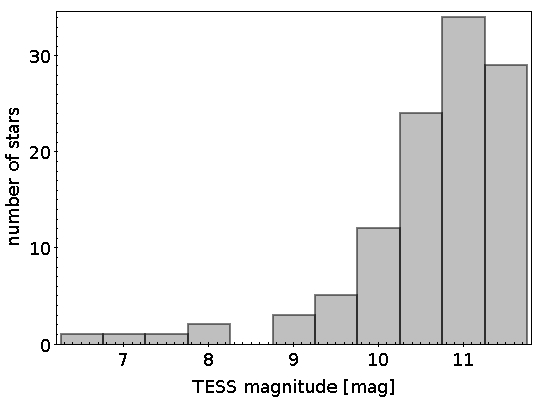
Figure 1: TESS magnitude distribution of all stars from the HZCat (Kaltenegger et al. 2019) with the “HZflag” set and $T\leq 11.5$ mag.

2.1 Calculation of stellar parameters

We calculated stellar parameters from the empirical relations in Mann et al. (2015) (using coefficients from Mann et al. 2016), Mann et al. (2019), Stelzer et al. (2016, S16) and Jao et al. (2018). These relations involve the color indices $V-J$ and $J-H$ as well as the absolute magnitude in the 2MASS $K_{s}$ band, $M_{K_{s}}$.

Therefore, we started by collecting optical and infrared photometry. We used the Gaia DR2 (Gaia Collaboration et al. 2016, Gaia Collaboration et al. 2018) and the Two Micron All Sky Survey (2MASS, Skrutskie et al. 2006) identifiers given in the HZCat for all sample stars. Gaia and 2MASS data were accessed via TOPCAT (Taylor 2005). We extracted 2MASS photometry by using the Table Access Protocol to perform an ADQL query based on the 2MASS IDs. For the Gaia DR2 data, we performed a coordinate-based multi-cone search in TOPCAT since in that way error estimates for the Gaia magnitudes could be collected, which are not available in the Gaia archive directly. The search was based on the TIC-coordinates (epoch J2000.0). The purpose of the cone search was not to find correct Gaia counterparts since they are already listed in the HZCat, but to retrieve the Gaia photometry and distances. Therefore, we could carry out the match to Gaia J2015.5 coordinates without a proper motion correction using a large search radius and subsequently identifying the correct Gaia source among the multiple matches by the help of the HZCat. With a match radius of $20^{\prime\prime}$ we recovered 108 out of the $112$ targets. For four targets with particularly high proper motions, ¿$1^{\prime\prime}$/yr (TIC 199574208, TIC 233193964, TIC 392572237 and TIC 359676790), we had to repeat the search with a larger match radius to catch the correct Gaia counterpart among the matches. The maximum match separation was $36.1^{\prime\prime}$.

In order to calculate $V$ magnitudes from Gaia photometry, we applied the empirical relation in Table 2 of Jao et al. (2018). This relation is valid in a range of $1.0\leq G_{\rm BP}-G_{\rm RP}\leq 4.0$, where $G_{\rm BP}$ and $G_{\rm RP}$ are the Gaia magnitudes in the blue and red photometer filters. All stars of our sample fulfill this requirement. For the distances, we used the inverse Gaia parallaxes. The results were subject to a reliability check following Lindegren et al. (2018), Appendix C, Equations (C.1) and (C.2). For most targets ($101$ out of $112$), we found the Gaia distances to be reliable. For these stars, the absolute $K_{\rm s}$-band magnitude, $M_{\rm K_{s}}$, was then determined using the distance modulus. Extinction can be neglected for these nearby stars. Since $11$ targets fail the Lindegren reliability check for the Gaia parallaxes, we also determined photometric distances, $d_{\rm phot}$. To this end, we calculated $M_{\rm K_{s}}$ from the empirical $M_{\rm K_{s}}$ versus $V-J$ relation given in Eq. 1 of S16. In order to obtain this relation, S16 performed a linear fit on the $M_{\rm K_{s}}$ versus $V-J$ diagram of $1078$ M dwarfs with trigonometric parallaxes given in the All-sky Catalog of Bright M Dwarfs (Lépine & Gaidos 2011). The $M_{\rm K_{s}}$ values determined by applying the S16 relation were then combined with the observed 2MASS $K_{\rm s}$ magnitude to yield $d_{\rm phot}$. Fig. 2 shows the relation of photometric distance to Gaia parallax distance for all targets. As expected, the ones with a large deviation between both distance values are found to have no reliable Gaia parallax according to the Lindegren quality conditions. Throughout this work we use the Gaia distances except for the stars that do not fulfill the abovementioned quality criteria. For these latter ones we use the photometric distances.

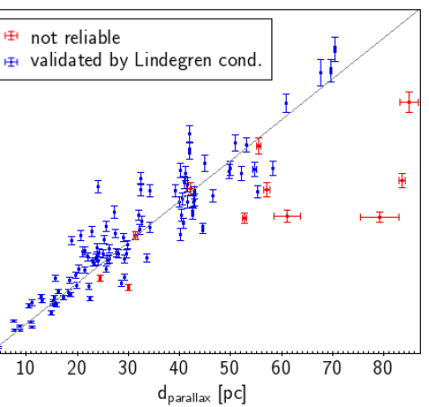
Figure 2: Relation of photometric distance and Gaia parallax distance. Stars failing the conditions of Lindegren et al. (2018) for a reliable Gaia parallax are marked in red. The gray line represents the 1:1-relation.

Bailer-Jones et al. (2018, BJ18) provide distance estimates for all $1.33$ billion stars that have parallax entries in Gaia DR2, using a distance prior that varies depending on the Galactic longitude and latitude of each star. We extracted the distance estimates provided by BJ18 and compared them to the inverse parallax for our sample stars. The deviations are marginal (with the maximum difference being $0.2$ pc), lending further credibility to the inverse parallaxes. One reason for the small differences is probably the fact that all stars within our sample are nearby (they all have distances $<100$ pc).

2.1.1 Spectral types

Spectral types were determined from $G_{\rm BP}-G_{\rm RP}$ and $G-G_{\rm RP}$ color indices using the online table A Modern Mean Dwarf Stellar Color and Effective Temperature Sequence maintained by E. Mamajek as an extension of Pecaut & Mamajek (2013). In that table, SpTs are given in steps of half-integer subclasses. We calculated for each star the expression

$$|(G_{\rm BP}-G_{\rm RP})_{*}-(G_{\rm BP}-G_{\rm RP})_{\text{SpT}}|\leavevmode\nobreak\ +$$

$$\hskip 113.81102pt|(G-G_{\rm RP})_{*}-(G-G_{\rm RP})_{\text{SpT}}|$$

where the subscript “$*$” denotes the color indices of the star and the subscript “SpT” the ones listed in the table for a particular SpT subclass. Then we assigned to each target the tabulated SpT that minimizes this expression. Fig. 3 shows the resulting SpT distribution of our sample.

We verified that the SpTs derived in that way are consistent with the ones obtained from the SpT-color relation provided by Raetz et al. (2020, R20) that was used in our previous works. R20 fitted a seventh order polynomial to the SpT versus $V-J$ relation extracted from the above-mentioned online table of E. Mamajek.

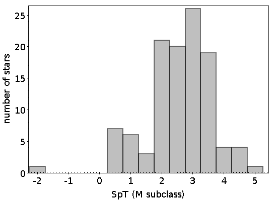
Figure 3: SpT distribution of our sample. Numbers denote M subclasses. -2 stands for SpT K8.

2.1.2 Mass and bolometric luminosity

Stellar masses ($M_{*}$) were obtained by applying the Markov chain Monte Carlo (MCMC) analysis described by S16: For each star, a set of 10000 $M_{K_{s}}$ values is drawn from a normal distribution with the observed value as mean and its error as standard deviation. The stellar mass is then calculated for all $10000$ values in the data set by applying Eq. 4 in Mann et al. (2019), using coefficients from their Table 6 for $n=5$, that is the case in which the relation is represented by a fifth order polynomial. Mann et al. (2019) denote this fifth order fit as the preferred one.

The stellar mass for each sample star is then determined as mean of the results of all $10000$ data sets for this star. To estimate the uncertainties, the standard deviations of the MCMC analysis are added in quadrature to the error given for the empirical relation.

Bolometric corrections in the $V$ band ($BC_{V}$) are given in the online table by E. Mamajek. We determined the bolometric corrections for our sample from this table, using SpTs as input.

The stellar parameters for all $112$ sample stars are listed in Table LABEL:tab:stellar_params_all. It comprises the TIC identifier (col. 1), the literature name (col. 2, obtained by searching SIMBAD for the main identifier of each star), Gaia DR2 (col. 3) and 2MASS (col. 4) identifiers, right ascension (RA, col. 5) and declination (Dec, col. 6) from the TIC, the TESS magnitude ($T$, col. 7), stellar mass ($M_{*}$, col. 8), distance ($d$, col. 9), SpT (col. 10) and quiescent luminosity in the TESS band ($L_{\rm qui,T}$, col. 11).

2.2 Common proper motion pairs

Binary stars require special treatment since for many of them, the separation between the target and its companion is on the order of the TESS pixel size ($21^{\prime\prime}$), and consequently the contribution of each star to the total flux of the TESS LC cannot be determined. This implies that characteristics observed in the LCs of targets with a visual companion might not originate in the target star itself. Additionally, close binaries are known to show higher flare rates than single stars, which might be a consequence of magnetic interactions between the components (e.g., Huang et al. 2020). Thus, close binaries might exhibit a behavior in terms of magnetic activity that is different from that of single stars. These magnetic interactions, however, only occur in case of small physical separation. The $12$ eclipsing M dwarf binaries studied by Huang et al. (2020), for example, have physical separations $\leq 0.25$ AU.

Our sample has been checked carefully for binary pairs, using two different approaches:

First, we compared the Gaia DR2 proper motion (PM) vectors for all Gaia sources within the TESS target pixel file (TPF) using a $164^{\prime\prime}$ radius (see Sect. 3.1) to the target’s PM. We consider objects with a deviation of less than $10$ % (in right ascension and declination, respectively) as companion candidates. Ten CPM pairs were identified with this procedure and verified through visual inspection in ESASky.

Second, the TIC coordinates of all sample stars were matched in TOPCAT with the Washington Double Star Catalog (WDS, Mason et al. 2020), using a match radius of 10^′′. This resulted in $19$ matches. All these $19$ targets except for two were confirmed to have a PM companion by visual inspection in ESASky. The first exception is TIC 198187008, for which a Gaia counterpart was not present in DR2 and could only be found in eDR3, where it still has no PM data and therefore cannot be confirmed to share the target’s PM. According to the WDS entry, the separation is extremely small ($0.4^{\prime\prime}$), which is probably the reason for the lack of Gaia data of the companion star. The WDS entry of TIC 198187008 is provided with the flag “V”, meaning “Proper motion or [an]other technique indicates that this pair is physical”. We flag TIC 198187008 as part of a CPM pair for the further analysis. The second target with a WDS entry for which no proper motion companion was found in ESASky is TIC 233193964. In this case, the separation of the system given in the WDS is between $230^{\prime\prime}$ and $300^{\prime\prime}$, and thus the companion is outside the TESS TPF. Therefore, the star was treated as a single star in the further analysis.

Comparing the results of the two methods, we found that $9$ of the $19$ WDS matches have also been identified as CPM pairs by our PM comparison. One target, TIC 142086813, was found from our PM comparison to have a companion while the WDS match yielded no result.

Thus, the total number of stars found to have a PM companion is $20$. Apart from TIC 233193964, one other binary has a very large separation of the two components: TIC 459985740 with $450^{\prime\prime}$. Treating these two targets as single stars due to the large separation to their companions, 18 stars remain to be flagged as part of a CPM pair for further analyses.

For two CPM pairs, both components are included in our HZCat sample: TIC 142086812 is the companion of TIC 142086813 and TIC 359676790 is the companion of TIC 392572237. Therefore, the $18$ stars within the sample that have a PM companion belong to $16$ CPM pairs.

Table A.2 lists for these $16$ CPM pairs the angular separation calculated based on Gaia DR2 coordinates and taken from the WDS in case of missing Gaia DR2 coordinates for the companion star. The table also contains the distance, $G_{\rm RP}$, stellar parameters ($R_{*}$, $M_{*}$, $T_{\rm eff}$) and SpT of both components except for two cases where the Gaia or 2MASS data of the companion object is incomplete. The stellar parameters of M-type companions were determined as described in Sect. 2.1. Small separations on the order of a few arcseconds lead to the CPM pair not being resolved in 2MASS. We caution that the empirical relations for stellar parameter calculations (cf. Sect. 2.1) cannot be applied to such unresolved cases. This also means that the stellar parameters of the corresponding sample stars might not be correct because the $J$, $H$ and $K_{\rm s}$ magnitudes for targets with unresolved PM companions given in the 2MASS catalog are the sum of the magnitudes of the CPM pair. Nearly all resolved companion objects are M dwarfs and span a SpT range from K9V to M5V. The only exception is the eclipsing binary CM Draconis that has a White Dwarf companion (see Appendix B for the treatment of this star). We calculated the physical separation for all CPM pairs within our sample and found a minimum value (apart from CM Dra) of about $14$ AU. This is more than two orders of magnitude above the maximum separation of the magnetically interacting binaries studied by Huang et al. (2020), which is, as mentioned above, $0.25$ AU. CM Dra is the only binary system within our sample that has a physical separation small enough for the components to interact magnetically ($\approx 0.02$ AU; see Appendix B for details).

3 Data analysis

In this work, we only considered data from the primary TESS mission (that is the first $26$ sectors) obtained in 2-minute cadence mode. In total, $1276$ 2-minute Pre-search Data Conditioning Simple Aperture Photometry (PDCSAP) TESS LCs and TPFs are available at the Mikulski Archive for Space Telescopes (MAST) for our $112$ sample stars. We filtered the data using the TESS quality flags: Almost all data points with flags $\neq 0$ were dismissed. We only kept “impulsive outlier” (value $512$, Bit $10$) as those data points might be part of a real flare and “cosmic ray detected in collateral pixel row or column” (value $1024$, Bit $11$).

Except for one star, TIC 229586790, all targets were observed in multiple TESS sectors (see Table LABEL:tab:rot_act). As explained in Sect. 2, this is a consequence of the target selection: We chose only stars from the HZCat that were observed long enough for TESS to probe the entire HZ for transiting planets.

3.1 Contamination analysis

TESS data are processed by a pipeline developed at NASA’s Science Processing Operation Center (SPOC, Jenkins et al. 2016). Due to the coarse TESS pixels that comprise an area of $21^{\prime\prime}\times 21^{\prime\prime}$ each, the aperture chosen by the SPOC pipeline often contains other stars besides the actual target. Even though the SPOC pipeline corrects for flux excess caused by star field crowding, these corrections cannot account for the possible variability of contaminating objects. Therefore, flares and the rotational signal in a LC with several stars inside the pipeline mask cannot be unambiguously ascribed to our target star. To identify such potential problematic cases, we conducted a contamination analysis based on fluxes in the Gaia $G_{RP}$ band since its wavelength range is a good approximation to the TESS bandpass (e.g., Gandolfi et al. 2018).

Our contamination factors provide a reasonable estimate to which extent another source might affect the LC. To calculate them, we proceeded as follows: First, we listed all Gaia sources that are located within a circular area of radius $164^{\prime\prime}$ (distance from center of TESS TPF to the corners, $0.5\cdot\sqrt{2}\cdot 11\cdot 21^{\prime\prime}\approx 163.3^{\prime\prime}$) around the target. Then, we checked for each Gaia source if it lies within a radius of $14.85^{\prime\prime}$ (half pixel diagonal) around the center of any of the pipeline mask pixels. Finally, the flux of all sources in the mask except for the target was summed up and the ratio of this sum to the target flux is defined as a contamination factor.

Table LABEL:tab:rot_act in the Appendix lists the mean, minimum and maximum contamination factors of all observation sectors for each target. There are $18$ stars with a maximum contamination $>10\%$. Ten of them are part of a CPM pair (see Sect. 2.2) with companions listed in Table A.2.

We discovered during the contamination analysis that three of our targets lie outside the TESS pipeline mask. Their LCs show many systematic effects that could be accidentally validated as flares in the LC analysis. These stars are TIC 359676790, TIC 392572237 and TIC 471015740. We did not consider these stars any further in the LC analysis. One reason for targets lying outside the mask might be a nearby contaminating source that the pipeline algorithm intended to exclude and then accidentally excluded also the target.

For the binaries in our sample listed in Table A.2, the maximum contamination factor of all TESS observation sectors is $>5$% for all systems resolved with Gaia. It is $>10$% in all except three cases (cf. Tab. LABEL:tab:rot_act). We note that for systems unresolved with Gaia, contamination is underestimated since the unresolved CPM pair as a whole is treated as the target source.

3.2 Rotation period search

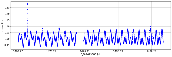
Figure 4: Example for a typical normalized PDCSAP LC, showing TIC220433364 in sector 6. The LC shows two humps of different height possibly resulting from two starspots on opposite sides of the star. Right before the $1478.27$ d timestamp, there is the typical gap that can be observed in every TESS LC due to a break in observation while downloading data to Earth (cf. Sect. 3.2).

The search for rotation periods ($P_{\text{rot}}$) was carried out using three different methods: autocorrelation function (ACF), Lomb-Scargle-Periodogram and sinefit, following our previous works (Stelzer et al. 2016, Raetz et al. 2020). In the version of the routine used for this work, the LC is only searched for periods up to a maximum length for which still two complete periods are covered by the duration of the LC, which is about $27$ d for individual TESS sectors. Thus, detectable periods are a priori limited to a maximum value of $13.5$ d. To calculate the generalized Lomb-Scargle-Periodogram (GLS), we used an algorithm by Zechmeister & Kürster (2009). The rotation period value resulting from GLS was then used as an initial guess for the sine-fit. The third method, ACF, faces some difficulties when it comes to TESS LCs due to the data gap in the middle of each observation sector (cf. example LC in Fig. 4). During this gap, data are transferred from the satellite to Earth and therefore no measurements can be recorded (cf. Schlieder 2017). As the ACF method needs equally spaced data points, we interpolated the gap in the middle as well as eventually occurring shorter gaps with a linear fit between the last data point before and the first one after the gap. Then, the ACF was calculated using the IDL routine A_CORRELATE. The rotation period was obtained by determining the time lag of the first peak in the ACF. The phase-folded LCs obtained from the three methods were plotted and evaluated by eye to verify the presence of rotational modulation.

One challenge in the search for stellar rotation periods in general is the fact that several LCs show “double-humps” resulting for instance from one larger and one smaller starspot on different hemispheres of the star (e.g., McQuillan et al. 2013). Fig. 4 shows an example of such a LC. For those cases, a by-eye inspection of the LC was necessary not only in order to decide if they show starspot variations but also to determine the correct value of the rotation period. The search algorithms often detected the distance between a smaller and larger hump as rotation period instead of the spacing between equal humps.

For a few targets, a rotation period was only found in some observation sectors while in others there was no rotational modulation evident or the differences between $P_{\textrm{rot}}$ values in different sectors were too big so that no clear cut result could be obtained. Fig. 5 shows as an example the LCs from two sectors of a star with not well-constrained rotation period. We disregard the periods of such cases in our work. We only consider rotation periods of stars with “reliable” $P_{\textrm{rot}}$ results and define “reliable” as follows: A rotation period is detected and is consistent in all observation sectors.

The adopted $P_{\rm rot}$ value for a given star was obtained from the results of all sectors in which it was observed as follows: First, we calculated the mean value of the $P_{\textrm{rot}}$ obtained from the three methods for each observation sector. In some cases, one method clearly failed to determine the correct rotation period. This became evident in the course of the visual inspection of the phase-folded LCs of all three methods, and the corresponding values were not taken into account. As a next step, we estimated errors for the averaged $P_{\rm rot}$ values of each sector using Eq. 2 of Lamm et al. (2004). This equation involves the width of the peak of the window function, $\delta\nu$. According to Roberts et al. (1987), this width can be approximated by $\delta\nu\approx 1/T$ with the length of the observation, $T$. This is possible for data sets with a sampling that is not too nonuniform. We used this approximation since all TESS LCs we analyzed have roughly the same length and the same regular two-minute cadence and are therefore uniform. The errors obtained from applying Eq. 2 of Lamm et al. (2004) were added in quadrature to the standard deviation of the results from the different methods to obtain the total error, $\Delta P_{\rm rot,tot}$, for each observation sector. The overall $P_{\rm rot}$ result for each target is then the weighted mean of all sectors, given by

$$<P_{\textrm{rot}}>=\sum_{\text{sectors}}\frac{P_{\textrm{rot}}}{\Delta P_{\textrm{rot,tot}}}\cdot\bigg{(}\sum_{\text{sectors}}\frac{1}{\big{(}\Delta P_{\textrm{rot,tot}}\big{)}^{2}}\bigg{)}^{-1},$$ (1)

and the corresponding error of the weighted mean is determined as

$$\Delta<P_{\textrm{rot}}>=\frac{1}{\sqrt{\displaystyle\sum_{\text{sectors}}\frac{1}{\big{(}\Delta P_{\textrm{rot,tot}}\big{)}^{2}}}}.$$ (2)

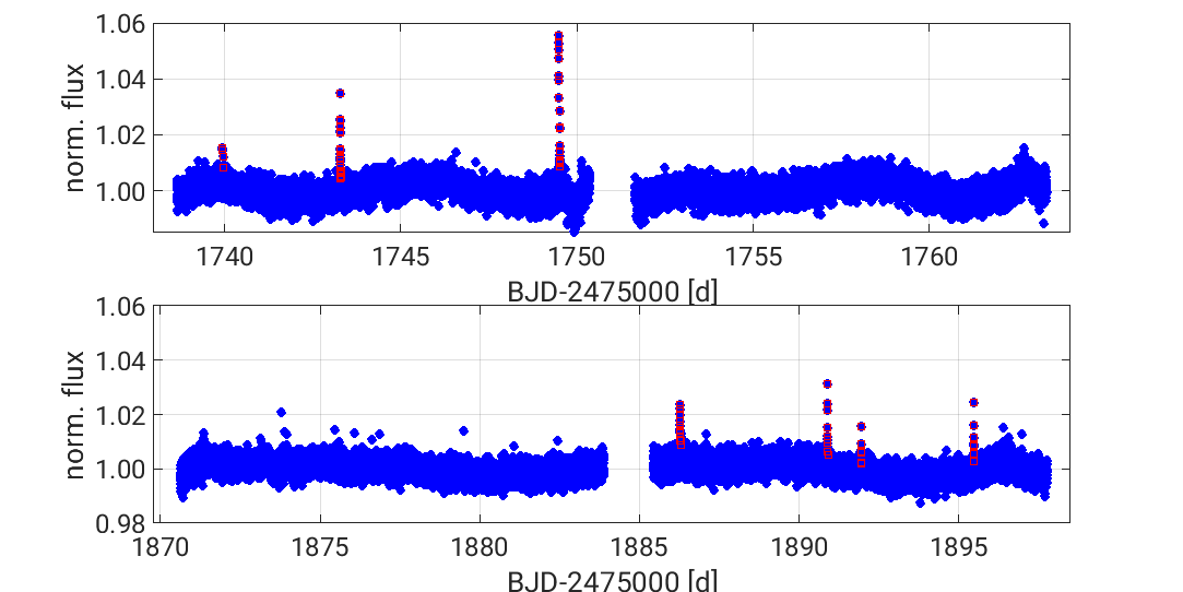
Figure 5: LC of TIC 320525520 in sector 16 (top panel) and sector 21 (bottom panel). Validated flares are marked. Both LCs show indications of rotational modulation, but the rotation period is not well constrained.

3.3 Flare detection and properties

3.3.1 Flare detection method

Our flare detection algorithm has been described by Stelzer et al. (2016) and Raetz et al. (2020) where it was applied to K2 mission long and short cadence data. Here, we briefly summarize the basic steps.

First, a “flattened and cleaned” LC is created in order to identify outliers as data points that deviate by more than three times the standard deviation of this flattened and cleaned LC ($S_{\textrm{flat}}$). To achieve this, the original LC is subject to an iterative boxcar-smoothing and cleaning process. In this procedure, after boxcar-smoothing is applied, the smoothed LC is subtracted from the original LC in order to remove the rotational modulation caused by starspots. Then, all data points with a deviation larger than $2S_{\textrm{flat}}$ are removed. This process is repeated three times with the boxcar width being reduced in each round. As a next step in the procedure, all parts of the LC with at least 3 consecutive data points of the original LC deviating by $\geq 3S_{\rm flat}$ each from the mean value of the flattened and cleaned LC are flagged as potential flares. Then, there are further criteria applied in order to decide if the potential flare is validated. In short, (1) The flare event must not occur right before or after a gap in the LC; (2) the flux ratio between flare maximum and last flare point must be $\geq 2$; (3) the flare maximum cannot be the last flare point; (4) the decay time has to be longer than the rise time; (5) a fit conducted using the flare template defined by Davenport et al. (2014) must fit the flare better than a linear fit.

3.3.2 Flare parameters

For all flares validated with these criteria, we determined the normalized peak flare amplitude, $A_{\textrm{peak}}$, namely the difference between peak flare flux and the flux of the smoothed, interpolated LC at the time of the flare peak, normalized to the mean flux of the LC. We further determined flare start, flare end and flare duration, $\tau_{F}$. This latter one is the time difference between first and last flare data point, where the last flare point is the last data point after the flare peak that deviates by $\geq 1S_{\textrm{flat}}$ from the mean value of the flattened and cleaned LC. Other flare parameters following from our analysis are the time of the flare maximum, the number of flare data points and the equivalent duration (ED). The ED is the integral of the LC under the flare data points. As the LC is normalized to the star’s mean flux, the unit of the ED is seconds (integrating a dimensionless quantity over time). It corresponds to the time span it would take for the star to radiate away the energy of the flare at its constant, quiescent luminosity (e.g., Hunt-Walker et al. 2012).

In order to get the flare energy, $E_{F}$, in units of erg, the ED is multiplied by the quiescent stellar luminosity in the TESS band, $L_{\rm qui,T}$. We calculated the luminosity as $L_{\rm qui,T}=4\pi d^{2}f_{\rm T}$, where $d$ is the distance and $f_{\rm T}$ the flux in the TESS band. The latter is obtained from the TESS magnitude ($T$) using the distance $d$ of the star, the filter bandwidth $W_{\textrm{eff}}=3898.68\leavevmode\nobreak\ \mathrm{\mathring{A}}$ and the zeropoint $ZP_{\lambda}=1.34\cdot 10^{-9}\leavevmode\nobreak\ \mathrm{erg/cm^{2}/s/\mathring{A}}$. Both values were taken from the website of the Spanish Virtual Observatory.

The flare amplitude in the TESS band ($\Delta L_{\rm F,T}$) in units of erg/s is calculated by multiplying the normalized flare amplitude $A_{\rm peak}$ with $L_{\rm qui,T}$. $\Delta L_{\rm F,T}$ is the luminosity increase caused by the flare at its maximum. The total stellar luminosity in the TESS band at the flare peak is obtained by adding $\Delta L_{\rm F,T}$ and $L_{\rm qui,T}$.

Flare rates, $\nu_{\rm F}$, were calculated by dividing the total number of validated flares (e.g., for a specific target or SpT) by the total observation time. The observation time for each individual LC is here defined as the difference between its first and last time stamp, subtracted by the summed up time spans of all data gaps. A data gap in this case is a sequence of at least two consecutive time stamps for which no flux measurements exist. This also applies to gaps at the beginning or end of the LC, in other words data gaps between sectors.

3.3.3 Cumulative flare energy frequency distribution

Cumulative FFDs are a common way to represent flare occurrence rates as a function of flare energies (e.g., Lacy et al. 1976, Hawley et al. 2014, Ilin et al. 2019, Raetz et al. 2020). The cumulative flare frequency, $\nu(>E_{\rm F,0})$, for a given flare energy, $E_{\rm F,0}$, is the total number of flares $N_{\textrm{flares}}(>E_{\rm F,0})$ with $E_{\rm F}\geq E_{\rm F,0}$ divided by the total observation duration of the target (see Table LABEL:tab:rot_act for the observation durations of our sample stars). To obtain the FFD, the cumulative frequencies are calculated and plotted against all values of $E_{\rm F,0}$ present in the flare sample.

Usually the FFDs are represented in double logarithmic form where they can be approximated by a linear relation:

$$\text{log}(\nu_{\rm F,0}):=\text{log}\bigg{(}\frac{N_{\textrm{flares}}}{\Delta t}\bigg{)}=\text{log}(\beta)+\alpha\cdot\text{log}(E_{\rm F,0})$$ (3)

(cf. Lacy et al. 1976), which is equivalent to the exponential power law $\nu_{\rm F,0}=\beta\cdot E_{\rm F,0}^{\alpha}$ in linear representation. It is known from observations of the Sun (e.g. Aschwanden et al., 2000) and other stars (e.g. Audard et al., 2000; Shibayama et al., 2013) that $\alpha$ is a negative value, since high-energy flares are less frequent than low-energy flares. In Sect. 4.6 we describe our analysis of the FFDs for the individual stars in terms of this power-law.

4 Results of rotation period and flare search

4.1 Rotation periods

Table 1: Basic stellar properties and results from the analysis of FFDs for the $12$ targets with reliable rotation period.

TIC ID	name	$<P_{\textrm{rot}}>$	SpT	$T$	$\log{(\langle E_{\text{min,th}}\rangle})$	$\nu_{\text{\rm flares,>Emin}}$	$\alpha$	log($\beta$)
		[d]		[mag]	[erg]	[d]-1	(cf. Eq. 3)	(cf. Eq. 3)
198187008		1.573$\pm$0.017	M3V	11.44	32.80	0.18	$-$1.17$\pm$0.04	37.69$\pm$1.13
199574208	CM Dra	1.268$\pm$0.015	M4V	10.36	31.87	0.14	$-$0.96$\pm$0.07	29.68$\pm$2.11
220433364	GJ2036 B	0.854$\pm$0.005	M4V	9.38	32.36	0.52	$-$1.19$\pm$0.05	38.51$\pm$0.86
233068870	LP71-82	0.280$\pm$0.001	M5V	10.25	31.41	0.37	$-$1.005$\pm$0.05	31.15$\pm$1.65
233532220	G227-45	0.851$\pm$0.004	M3V	11.41	32.63	0.10	$-$0.84$\pm$0.06	26.56$\pm$1.98
233738219		1.316$\pm$0.010	M3.5V	10.88	32.02	0.07	$-$0.84$\pm$0.11	25.88$\pm$3.43
272232401	L34-26	2.831$\pm$0.055	M3V	8.92	31.98	0.63	$-$0.86$\pm$0.03	27.29$\pm$0.80
272785770		3.936$\pm$0.087	M2.5V	9.89	32.62	0.28	$-$1.14$\pm$0.04	36.86$\pm$1.03
287350461		0.325$\pm$0.001	M4V	11.29	32.13	0.07	$-$1.08$\pm$0.26	33.48$\pm$8.32
359313701		1.791$\pm$0.018	M3.5V	10.73	32.38	0.29	$-$1.00$\pm$0.06	31.95$\pm$1.06
406857100	GJ4053	0.522$\pm$0.002	M4.5V	10.39	31.35	0.11	$-$1.27$\pm$0.13	38.92$\pm$4.26
441734910		1.357$\pm$0.010	M3V	11.39	32.42	0.26	$-$0.85$\pm$0.03	27.23$\pm$1.04

A total of $12$ stars in our sample of $109$ (that is $112$ minus the three excluded based on the contamination analysis, cf. Sect. 3.1) have a “reliable” rotation period according to our definition in Sect. 3.2.

Table 11 lists the adopted $P_{\textrm{rot}}$ values for these $12$ stars together with the results from the analysis of their FFDs, which are discussed in Sect. 4.6. The $P_{\rm rot}$ results are the weighted mean of the measurements in all observation sectors of the star, derived as explained in Sect. 3.2. We notice that all $12$ targets are fast rotators with $P_{\rm rot}$ values ranging from $0.28$ d to $3.93$ d. Example LCs of one observation sector for each of them are shown in Appendix C.

Among these $12$ stars with reliable $P_{\rm rot}$ there are four that are part of a CPM pair of which two have a maximum contamination factor of all observation sectors that is $>10$ %. The other two systems are unresolved in Gaia DR2, and thus the contamination is underestimated. One additional star has a maximum contamination factor $>10$ % without being part of a CPM pair (cf. Table LABEL:tab:rot_act in the Appendix), meaning the contamination is from an unrelated neighboring Gaia source.

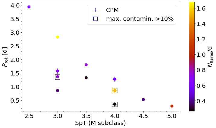
Figure 6: Relation between SpT and rotation period for the $12$ stars with reliable $P_{\textrm{rot}}$. The flare rate of each target is color-coded. There is a clear tendency of later M-type stars having shorter $P_{\textrm{rot}}$ values.

As stars evolve with time, they experience changes in their rotation. During the pre-main-sequence (pre-MS) phase, the rotation period is roughly constant (e.g., Irwin et al. 2011, Johnstone et al. 2021). The spin-up that would follow from the star’s contraction is opposed by star-disk interactions that remove angular momentum (e.g., Allain 1998). After the circumstellar disk has disappeared, rotation is slowed down as angular momentum is carried away by magnetically driven stellar winds. The timescale over which this spin-down of rotation takes place depends on the stellar mass (e.g., Irwin et al. 2011). Fig. 6 displays $P_{\rm rot}$ versus SpT in which a strong tendency of later M-type stars having shorter rotation periods can be observed. Such a trend can be explained by the increase of the spin-down timescale for lower stellar masses (e.g., Reiners & Basri 2008, Scholz 2013), which implies that stars of later SpTs are more likely to still be in a relatively fast rotation state.

4.2 Flares

Table 2: Physical parameters of all validated flares calculated as described in Sect. 3.3.2.

TIC ID	flare start	flare max	$A_{\text{peak}}$	$\log(\Delta L_{F,T})$	ED	log($E_{\text{flare}}$)
	[BJD-2475000]	[BJD-2475000]		[erg/s]	[s]	[erg]
233068870	1813.016182	1813.016182	0.008	28.38	3.40	31.01
”	1816.317568	1816.317568	0.011	28.52	3.47	31.02
”	1817.030065	1817.030065	0.020	28.77	8.64	31.41
”	1817.062009	1817.062009	0.008	28.37	2.16	30.81
”	1817.417563	1817.418952	0.014	28.61	15.88	31.68
”	1818.221727	1818.221727	0.034	28.01	7.57	31.3
”	1818.838391	1818.838391	0.024	28.86	7.68	31.36
…	…	…	…	…	…	…

The sample contains $55$ targets for which our flare search algorithm detected and validated flares. Three of them had to be excluded from the analysis since the targets lie outside the pipeline mask, as we discovered in the contamination analysis (cf. Sect. 3.1). All validated flares were subject to visual inspection, which resulted in rejecting the flare results of an additional $17$ targets. For a majority of those, the algorithm validated only one single event as a flare and this event was clearly an artifact. Among these $17$ stars, only TIC 142086813 had several events validated as flares which were all dismissed as artifacts after visual inspection. After the visual inspection, a total of $2532$ validated flares remain, occurring on 35 targets, that is we detected flares on $\approx 32$% of the total sample.

Seven of the $35$ flaring stars in our sample have a PM companion, cf. Table A.2 in the Appendix. For four of these seven, the maximum contamination factor of all sectors is greater than $10$ % and two systems are unresolved by Gaia. An additional five of the $35$ flaring stars have maximum contamination factors $>10$ % without being part of a CPM pair.

All flare parameters are available in an online table that comprises the TIC ID (col. 1), the time of flare start and maximum (cols. 2 and 3), normalized ($A_{\rm peak}$, col. 4) and absolute ($\Delta L_{\rm F,T}$, col. 5) flare amplitude, equivalent duration (ED, col. 6) and flare energy ($E_{\rm flare}$, col. 7). Table 2 shows an excerpt of this flare parameter table.

4.3 Flares and rotation

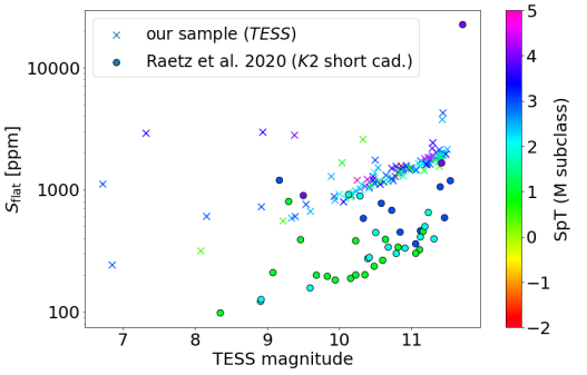
Figure 7: Relation between the standard deviation of the flattened and cleaned LC ($S_{\rm flat}$) and TESS magnitude. Circles represent the $S_{\rm flat}$ in K2 short cadence LCs of the M dwarf sample presented by Raetz et al. (2020). The conversion between K2 and TESS magnitudes is described in Appendix D.

All targets with reliable $P_{\rm rot}$ also show flares, which is not surprising given that they have measurable starspots that indicate significant magnetic activity. In fact, $2138$ out of $2532$ validated flares occur on the $12$ targets with unambiguous rotation periods. The remaining $394$ flares partly occur on stars that show some indication for rotational modulation (described in Sect. 3.2) and some occur on targets without any indication of starspot modulation. From their Kepler flare studies, Yang & Liu (2019) report that for $291$ out of $3420$ flaring stars the LCs show no starspot variations. The authors give as possible explanations that the star’s rotation axis might be inclined with respect to the observer’s line of sight or that starspots might be located near the poles of the star and, therefore, cause much less rotational modulation in the LC as if they were near the equator. As far as our work is concerned, an additional plausible reason for observing flares but no starspot modulation in some LCs is the limited photometric precision and resulting high scatter in TESS LCs. The standard deviation of the LC after subtraction of rotational modulation and flares, $S_{\rm flat}$, (see Sect. 3.3), is plotted for our sample versus TESS magnitude in Fig. 7. Almost all targets are observed in multiple TESS sectors and each sector is divided into two segments due to the data gap in the middle (cf. Sect. 3.2), such that we obtain two $S_{\rm flat}$ values for each sector’s LC. The $S_{\rm flat}$ for each target in Fig. 7 is the mean of all values obtained from its TESS LCs.

For comparison, Fig. 7 also shows the $S_{\textrm{flat}}$ values in K2 short cadence LCs of the M dwarf sample presented by Raetz et al. (2020). In order to be able to compare the $S_{\textrm{flat}}$ between the TESS and K2 sample, we derived an empirical magnitude conversion between the TESS and Kepler band. This procedure is described in Appendix D. The K2 stars from Raetz et al. (2020) are plotted in Fig. 7 at their derived TESS magnitude obtained from Eq. 7.

For both the TESS and the K2 sample, $S_{\rm flat}$ increases for stars with fainter magnitudes, that is the signal to noise ratio worsens. Our $S_{\rm flat}$ values are clearly higher than the ones of Raetz et al. (2020) for K2 short cadence LCs. The difference is on average $560$ ppm.

4.4 Relation between flare rate and SpT

When investigating a correlation of flare rate and SpT, detection biases have to be taken into account. Specifically, only flares with a peak amplitude in the TESS band of $\Delta L_{\rm F,T}>3S_{\rm flat}\cdot L_{\rm qui,T}$ can be detected for each target. In fact, the detection threshold is even higher than this since not only one data point is required to lie above $3\sigma$, but three consecutive data points (cf. Sect. 3.3). Thus, the exact amplitude limit depends on the flare shape. A second approach is therefore to constrain the detection threshold in terms of flare energy instead of $\Delta L_{\rm F,T}$. This is discussed further in Sect. 4.6. For the discussion of detection biases which is the topic of this section, the amplitude threshold is, however, a useful criterion. The aim of the following considerations is to assess whether the detection threshold is in any way correlated with the SpT.

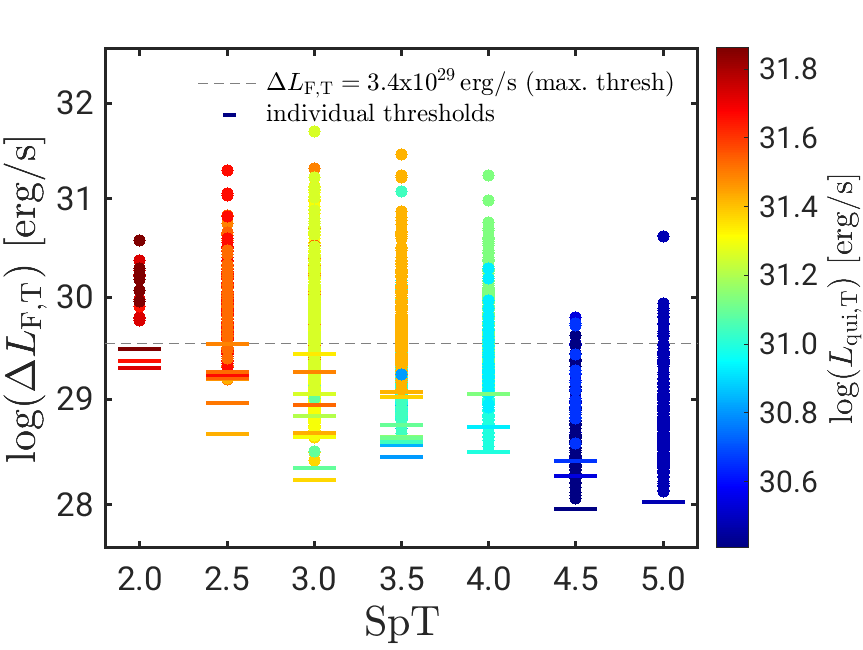
Figure 8: Relation between peak flare amplitude in the TESS band, $\Delta L_{\rm F,T}$, and SpT. The minimum value of $\Delta L_{\rm F,T}$ that could be detected for each target is represented by a “_” marker. The gray dashed line marks the highest of the flare amplitude detection thresholds for all flaring stars in this sample of $L_{\text{max,th}=3.4\cdot 10^{29}}$ erg/s (see Sect. 4.4). The color code visualizes the expected correlation between $L_{\textrm{qui},T}$ and SpT.

Firstly, stars with a fainter apparent magnitude have a higher noise level, that is a larger $S_{\rm flat}$ (cf. Fig. 7). The bias regarding the SpT dependence of activity following from this $S_{\rm flat}$ versus $T$-mag relation is probably small as there is no evident correlation between SpT and TESS magnitude within the sample (cf. color coding in Fig. 7).

Quiescent luminosity and SpT are, however, strongly correlated. Main-sequence stars of later M SpT subclasses have by definition a lower $L_{\rm qui,T}$ and, therefore, a lower flare detection threshold. Consequently, flares with lower amplitudes can be detected. In Fig. 8, flare amplitudes are plotted versus SpT. The flare detection threshold of each star is represented by a horizontal bar marker. We found the highest of these detection thresholds to be $L_{\rm max,th}=3.4\cdot 10^{29}$ erg/s. Flares with higher amplitudes can be detected on all 35 flaring stars of our sample. Stars of the latest SpT class ($\geq$ M4.5) show only a few flares above this threshold, but they have many fainter flares that are undetectable for earlier-type stars.

We further examine this detection bias and the result after its removal in Fig. 9. It shows the flare rate for all flaring stars as a function of SpT considering only the flares with an amplitude greater than $L_{\rm max,th}$. In total, $30$ of the $35$ flaring stars within our sample show flares above the sensitivity threshold. The energy of the largest flare for each star is chosen for the color-coding since it is a straight-forward indicator for flare energy and free from evident detection bias (in contrast to lower flare energies). Within each SpT bin, the maximum observed flare energy is correlated with the flare rate. Moreover, the stars with reliable rotation periods (squares) have the highest flare rates (see also Sect. 4.3) and higher energies of their largest flares. Further, it can be observed in Fig. 9 that the flare rate sharply drops for stars of SpT M2 and earlier and thus this is not an effect of the sensitivity bias. For stars of SpT M4.5 and M5, the amplitude cutoff at the maximum detection threshold eliminates nearly all flares. Fig. 8 already shows that these stars hardly show flares with amplitudes above the common threshold.

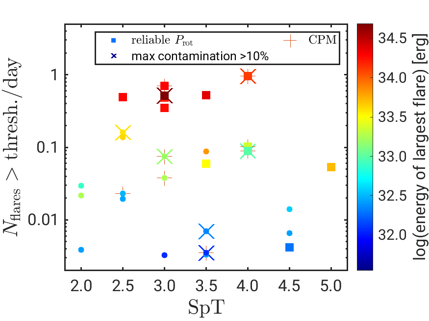
Figure 9: Relation between flare rate and SpT. The $12$ targets with flares and a reliable rotation period are shown with square markers. The energy of the largest flare is color-coded for each target. Only flares with amplitude $\Delta L_{F,T}>L_{\rm max,th}=3.4\cdot 10^{29}$ erg/s are considered, to account for the sensitivity detection biases (cf. Sect. 4.4).

The SpT distribution of the $30$ stars with flares above $L_{\rm max,th}$ is plotted in Fig. 10 together with that of all $109$ stars considered in the analysis. It is evident that the ratio of stars showing flares above the detection threshold to non-flaring stars is higher for later M SpT subclasses. In particular, stars earlier than SpT M2 do not show any flares above the threshold - despite the fact that their numerical representation in the sample is comparable or even slightly higher than that of M4 to M5 stars. Overall, three groups seem to stand out, namely stars with (i) SpT $\leq$ M2, (ii) M2 $<$ SpT $\leq$ M4, and (iii) SpT $>$ M4. In Table 3 we summarize the flare statistics for these three SpT ranges considering only events above the threshold $L_{\rm max,th}$. To obtain the total observation time for calculating the flare rates, the observation times of all targets considered in the analysis (cols. 3 and 4) or the subsample of targets exhibiting flares above $L_{\rm max,th}$ (cols. 5 and 6) for the respective SpT range are summed up. We caution that these results is based on low-number statistics.

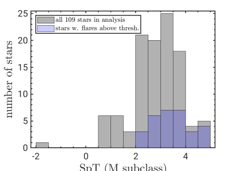
Figure 10: SpT distribution of all $109$ targets considered in the LC analysis and the $30$ stars showing flares above the maximum amplitude threshold of $3.4\cdot 10^{29}$ erg/s. (cf. Sect. 4.4). Numbers on the x-axis label M SpT subclasses, where “-2” stands for SpT K8.

4.5 Relation between flare amplitude and duration

Figure 11: Relative flare amplitude versus flare duration for the 8 stars with reliable $P_{\rm rot}$ that have no PM companion. The orange and turquoise lines are linear fits performed in different SpT ranges as indicated in the legend. Left panel: Normalized peak flare amplitude. Right panel: Peak flare luminosity amplitude. Relations from Hawley et al. (2014) and Raetz et al. (2020) are overplotted for comparison; see Sect. 4.5 for details.

Table 3: Number of flares and flare rates.

		all stars		flaring stars
	$\Sigma$ $N_{\textrm{flares}}$	$N_{\textrm{targets}}$	$\nu_{\textrm{flares}}$	$N_{\textrm{targets}}$	$\nu_{\textrm{flares}}$
	($>$ the thresh.)		[d-1]		[d-1]
SpT $\leq$ M2	16	37	0.001	3	0.019
M2 $<$ SpT $\leq$ M4	1240	67	0.070	23	0.207
SpT $>$ M4	19	5	0.015	4	0.020

The left panel of Fig. 11 shows the normalized flare amplitude $A_{\rm peak}$ versus flare duration $\tau_{\rm F}$, the right panel shows the same plot for the absolute flare amplitude $\Delta L_{\rm F,T}$.

The black dashed line is a linear relation that we extracted from Fig. 10 in Hawley et al. (2014), and the black dotted lines represent the lower and upper envelope of this relation. These authors analyzed the relation between flare amplitude and duration for GJ 1243, an M4 dwarf with a rotation period of $0.59$ d in Kepler short cadence observations. This star has become a benchmark for flare studies and its applications to exoplanets (Davenport et al., 2020; Tilley et al., 2019) because of a combination of favorable properties including its its proximity ($12$ pc; Gaia Collaboration, 2020), long coverage with Kepler and elevated activity level. The flare rate of GJ 1243 was found by Hawley et al. (2014) to be intermediate to high when compared to other M dwarfs. The general result for GJ 1243 of longer flares having a higher relative amplitude, $A_{\textrm{peak}}$, is also present in the flare data of our HZCat sample. However, with respect to GJ 1243 higher amplitudes for given flare duration are measured in our sample.

We performed linear fits using only the single stars and separating our sample into two SpT bins ranging from M2.5$-$M3.5 and from M4.5 $-$M5. No M4 stars were considered since they all have PM companions. According to Fig. 9, the flare rate drops after SpT M4, but the linear fits performed for the two SpT subranges of our sample (orange and turquoise lines in Fig. 11) are nearly indistinguishable for the normalized flare amplitude versus duration (left panel). The activity level of the stars, therefore, is unlikely to be responsible for the difference in our $A_{\rm peak}-\tau_{\rm F}$ relation with respect to GJ 1243. It might, instead, be due to instrumental differences with an impact of the noise level on the measured flare shape (see below and Sect. 6.1.3).

After transforming the amplitudes to absolute values, $\Delta L_{\rm F,T}$, we again fitted the two selected SpT subsamples of our HZCat targets. Contrary to $A_{\text{peak}}$ versus $\tau_{F}$, the relation between flare duration and absolute flare amplitude, $\Delta L_{\rm F,T}$, is different for the two SpT subsamples, with the fit for earlier SpTs shifted upward as a result of the higher quiescent luminosities of earlier-type stars. This represents the same detection bias that is seen in Fig. 8. The black dashed line again refers to the results of Hawley et al. (2014) for GJ 1243 that we have converted from normalized to absolute flare amplitudes by adding the logarithm of the quiescent luminosity of GJ 1243 in the Kepler band, $\log L_{\rm Kep}$ [erg/s]=30.67 (cf. Hawley et al. (2014), Table 2). The relation of Hawley et al. (2014) is shifted toward lower absolute flare amplitudes with respect to both our subsamples. Since GJ 1243 has SpT M4, in between our two bins, this cannot be an effect of SpT or $L_{\rm qui}$. Thus, the flares we detected for the targets of this work have higher absolute and normalized amplitudes than GJ 1243 in the Kepler short cadence analysis of Hawley et al. (2014). Hence our sample has on average a different amplitude-duration relation than GJ 1243.

The green dotted line in Fig. 11, right panel is the amplitude-duration relation from Raetz et al. (2020) (R20, their Eq. 4), derived from K2 short cadence observations of 56 bright, nearby M dwarfs (SpT K7 to M6) and it is also shifted upward with respect to GJ 1243. In contrast to our sample, the sample of R20 comprises several slow rotators (i.e., $P_{\text{rot}}>10$ d) and a larger fraction of early-M-type stars (SpT K7 to M1). Our range of measured flare durations and amplitudes is comparable to that of R20. We conclude that the flares of GJ 1243 constitute the lower end of the amplitudes for the star’s SpT and $P_{\rm rot}$ value or - equivalently - that its flares last longer for given amplitude. This might be due to a lower noise level in the data for GJ 1243, which is from the main Kepler mission as compared to the K2 data from Raetz et al. (2020) and the TESS mission from our work. In fact, tests with simulated flares show that for the recovered events the flare durations are more severely underestimated than the amplitudes, because part of the flare remains buried in the noise.

4.6 Flare frequency distributions

Fig. 12 shows the FFDs of all $35$ flaring stars with a color-code for the rotation periods of the $12$ stars with reliable $P_{\text{rot}}$. In Sect. 4.3 we have discussed that stars with reliable $P_{\text{rot}}$ show higher flare rates and this is also evident here, namely their FFDs lie above those of stars without reliable $P_{\rm rot}$. In fact, the vast majority of the $>2500$ flares occur on the $12$ stars with reliable $P_{\rm rot}$. The FFD power law fit defined in Sect. 3.3.3 was, therefore, only conducted for these $12$ targets.

A quantitative evaluation of the FFDs through a power law fit depends crucially on the determination of the completeness limit, as the detection of flares depends on the individual noise level of the LC, which is characterized by the standard deviation, $S_{\rm flat}$, defined in Sect. 3.3.1. Each FFD thus has an observation-specific cutoff flare energy, $E_{\rm min,th}$, below which not all events are detected. This usually translates into a flattening of the FFD for flare energies $<E_{\rm min,th}$.

We determined $E_{\rm min,th}$ for each of the $12$ stars and for each of its TESS LCs separately using the method described by Raetz et al. (2020). Our technique employs the flare template of Davenport et al. (2014) with an assumed flare duration of $360$ s, and examines the amplitude of flares that have $3$ data points above the detection threshold of $3\,S_{\rm flat}$, namely our criterion for flare detection from Sect. 3.3.1. The energy of this synthetic flare with an amplitude just high enough that it would be detected by our flare search algorithm is then the energy completeness threshold, $E_{\rm min,th}$.

We note that for each star the FFD fit comprises flares from all TESS sectors in which the star was observed, and consequently there is not a unique value of $E_{\rm min,th}$ associated with a given star but all flares from each of the sectors $s$ that have their energy fulfilling $E_{\rm f,s}>E_{\rm min,th,s}$ are considered in the power-law fit. In practice, for a given star the energy thresholds from different sectors are all within a small range.

In the fitting we took account of Poisson uncertainties on the flare rates as described by Hawley et al. (2014), that is the flare number is assumed to be Poisson-distributed as a function of flare energy, thus

$$\qquad\Delta\nu_{\text{flares}}=\frac{\sqrt{N_{\textrm{flares}}}}{t_{\textrm{obs}}},$$ (4)

with the flare frequency $\nu_{\rm flares}$ in units of d^-1. In logarithmic representation, the error becomes

$$\qquad\Delta\text{log}(\nu_{\text{flares}})=\Delta\nu_{\text{flares}}\cdot\nu_{\text{flares}}^{-1}=$$

$$\qquad\bigg{(}\frac{\sqrt{N_{\textrm{flares}}}}{t_{\textrm{obs}}}\bigg{)}\cdot\bigg{(}\frac{N_{\textrm{flares}}}{t_{\textrm{obs}}}\bigg{)}^{-1}=\frac{1}{\sqrt{N_{\textrm{flares}}}}$$

by error propagation. This consequently gives larger errors in the cumulative rates of high flare energies due to the smaller number of flares found there.

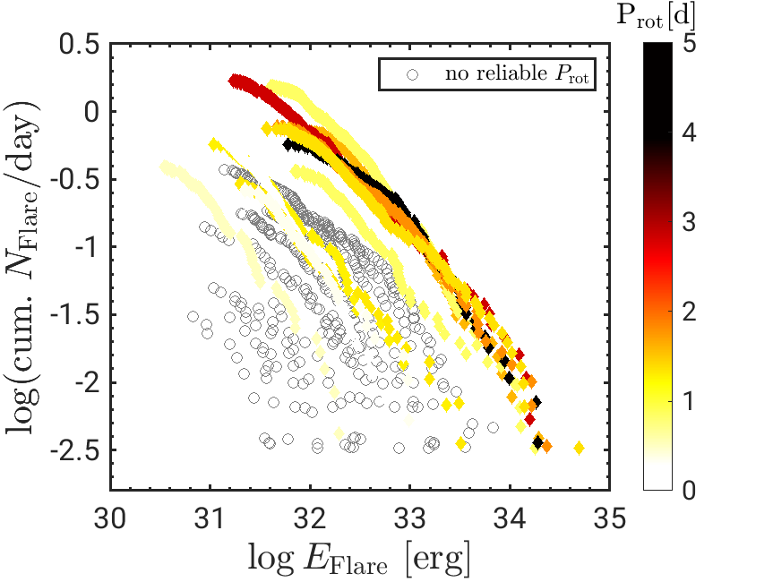
Figure 12: Cumulative distribution of flare energies for all $35$ flaring stars; the $12$ stars with reliable $P_{\rm rot}$ are highlighted in color.

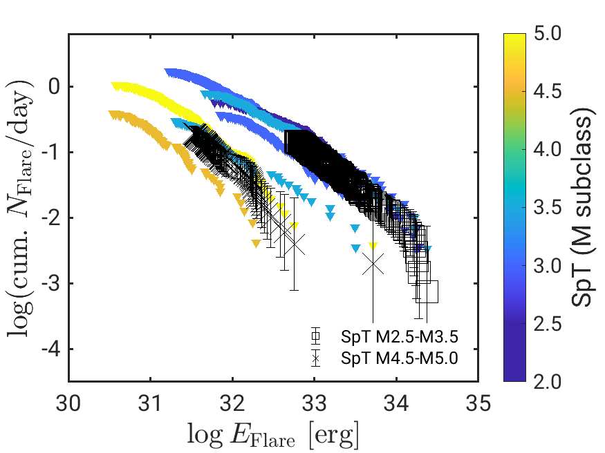
Figure 13: FFDs of stars with reliable $P_{\text{rot}}$ without the five stars with PM companions or a maximum contamination in all TESS sectors $>10$ %. Black square and cross symbols represent the average FFDs for the earlier and later M SpT subclass. Error bars for these average FFDs result from Eq. 4. Since the stars considered in the SpT-averaged FFD have a range of completeness limits, $E_{\rm min,th}$, for each of the two distributions the fits have been limited to flares with energy above the highest value of the $E_{\rm min,th}$ of all stars in the respective sample.

Table 4: FFD power law slopes and y-axis offsets for the two SpT-averaged TESS FFDs (see Sect. 4.6) and the corresponding X-ray FFDs constructed as described in Sect. 5.2.

	power law slope ($\alpha$ from Eq.3)		y-axis offset ($\log{\beta}$ from Eq.3)
SpT range	M2.5-M3.5	M4.5-M5.0	M2.5-M3.5	M4.5-M5.0
TESS (black)	$-1.20\pm 0.04$	$-1.05\pm 0.06$	$38.68\pm 1.28$	$32.25\pm 1.89$
X-ray (red)	$-0.85\pm 0.03$	$-0.74\pm 0.04$	$26.31\pm 0.89$	$21.48\pm 1.28$

We computed average FFDs for the same two SpT ranges used in Fig. 11 for studying the flare amplitude$-$duration relation. Eliminating from the subsample of $12$ stars with reliable $P_{\rm rot}$ those with PM companions or a maximum contamination factor $>10$ % leaves a sample of five stars for the M2.5$-$M3.5 range and two stars for M4.5$-$M5. The average FFDs for each of these two SpT subgroups have been constructed from the flares of all stars that belong to the respective group. Hereby, we considered among all flares from all sectors for all stars in the respective SpT subgroup only those above the highest $E_{\rm min,th}$ threshold, combining them into a single FFD. The use of this conservative value for the energy threshold ensures that no additional artificial substructures are introduced into the FFDs as a consequence of the different noise levels of the stars. These average FFDs for the two SpT subgroups are shown in Fig. 13 with black symbols, together with the FFDs of the seven individual stars that were taken into account.

Fig. 14 shows again the same average TESS FFDs in the SpT ranges M2.5$-$M3.5 and M4.5$-$M5. Overlaid are the power law fits, the parameters of which are listed in Table 4. We also display the linear fits obtained by Ilin et al. (2019) for Pleiades stars in similar $T_{\rm eff}$ ranges. The $T_{\rm eff}$ ranges given in the legend for our two SpT bins correspond to the ranges spanned by the stars in the respective bin. While our slopes are similar to those for the Pleiades sample, our earlier SpT bin has a significant upward shift with respect to the corresponding Pleiades flare distribution. This could be due to a different rotation period distribution, and hence activity level, of the considered stars. The different observing cadence to which the two data sets refer may also play a role: Ilin et al. (2019) have used K2 long cadence LCs, and Raetz et al. (2020) found that flare rates are lower in long-cadence as compared to short-cadence data. We show the Pleiades power-laws down to the energy thresholds given by Ilin et al. (2019). As can be seen, the $E_{\rm min,th}$ values for our field M dwarfs are more sensitive than the ones for the Pleiades, especially for the later SpT bin, likely as a result of the closer distance of our sample, the different data cadence and differences in the flare detection methods.

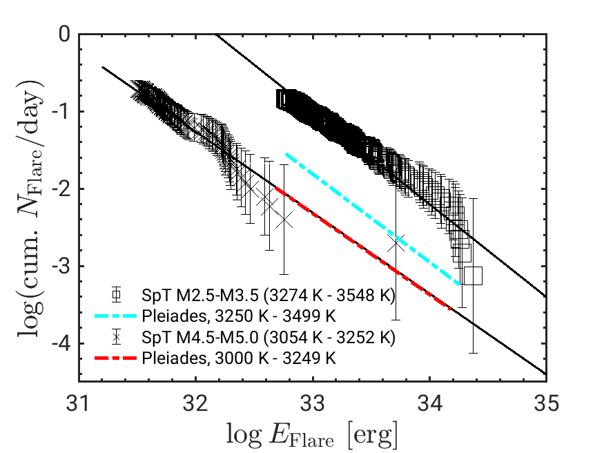
Figure 14: Average FFDs for two SpT ranges as in Fig. 13 (black data points) but here together with power law fit. The fit parameters are listed in Table 4. The linear fit of the Pleiades FFDs based on K2 long cadence data in two similar SpT ranges is taken from Table 4 of Ilin et al. (2019) for energies above the completeness limits given in their work.

4.7 Flares of TOIs and confirmed planet host stars within our sample

Table 5: Stars with confirmed planets or TOIs and information on flares and rotation period.

TIC ID	other	comment	flares?	$\mathrm{P_{\text{rot}}}$?
198211976	TOI-2283	–	–	–
233193964	GJ 687	2 RV det. pl.	$\checkmark$	–
235678745	TOI-2095	–	–	–
260004324	TOI-704,	conf. pl.	–	–
	LHS 1815
260708537	TOI-486	–	$\checkmark$	–
272232401	L 34-26	direct imaging	$\checkmark$	$\checkmark$
307210830	TOI-175,	4 conf. pl.	$\checkmark$	–
	L 98-59
377293776	TOI-1450	–	$\checkmark$	–

We downloaded the list of all TOIs and confirmed TESS planets from the NASA exoplanet archive and matched them with our sample. Among our $112$ stars there are eight TOIs, four of which have confirmed planets. Of these four, two have planets discovered by TESS: The M2 dwarf TIC 260004324 alias TOI-704 (Gan et al. 2020) and the M3 dwarf TIC 307210830 (L 98-59, TOI-175). The latter hosts a system of four planets (e.g., Kostov et al. 2019, Cloutier et al. 2019, Demangeon et al. 2021). A third star, TIC 233193964 (GJ 687), has two planets that have been detected through radial velocity measurements. One was already known before the TESS mission (Burt et al. 2014), the other one has been discovered recently (Feng et al., 2020). TIC 272232401 was found to host a planet with a wide orbital separation of $7506^{+5205}_{-2060}$ AU (Zhang et al., 2021) which was discovered by direct imaging.

Table 5 gives an overview for which of the eight TOIs and planet hosts we detected flares and rotation periods. The detailed results of our analysis, such as the $P_{\text{rot}}$ values and the flare rates with a cutoff at the maximum amplitude threshold of $3.4\cdot 10^{29}$ erg/s (cf. Sect. 4.4), can be found in Table LABEL:tab:rot_act. Flare rates of all TOIs with two-minute cadence TESS LCs have been presented by Howard (2022); this list should include the TOIs from our Table 5 but their full target list is not available yet.

5 Calibrating X-ray flare energies

The part of the stellar radiation that has the most important effects on planets is the high-energy UV and X-ray emission. Especially crucial is the variability of the stellar irradiation, both the amount of the brightness changes (flares) and the frequency of the events. However, only a very limited number of UV and X-ray observations of M dwarfs during flare events are available. Therefore, an indirect way must be found to estimate the energy of XUV flares that reaches the planet.

Combining the extensive data base of optical flares detected with TESS in our sample with a collection of simultaneous optical and X-ray observations of flares on M dwarfs we propose here a calibration from the radiative output of flares in the optical TESS band to XMM-Newton’s X-ray band. Arriving from the observed TESS flare properties at an estimate of the properties of the same events in the X-ray band is a multistep procedure. Since – to the best of our knowledge - there are no simultaneous TESS and X-ray observations of M dwarf flares available we take a detour involving K2 data. We first calibrate the TESS flare properties to their K2 equivalents making use of an early-M dwarf observed with both TESS and K2 (Sect. 5.1.1), then we estimate the X-ray output of the flares in Sect. 5.1.2 making use of a simultaneous K2 and XMM-Newton observation of the Pleiades (Guarcello et al. 2019) and a second simultaneous Kepler and XMM-Newton flare study by Kuznetsov & Kolotkov (2021). In Sect. 5.1.3, we combine the results to estimate the X-ray energy of our observed TESS flares. Finally, we construct X-ray FFDs based on these estimates in Sect. 5.2.

5.1 Simultaneous multiwavelength observations of M dwarf flares

5.1.1 From TESS to K2

In the course of a comparative study of TESS and K2 observations in a sample of M dwarfs observed with both missions (Raetz et al., in prep.), wecomputed the frequency distributions of the flare energies derived from both instruments. When comparing the TESS and K2 flare rates one must be aware that there is a time-lapse of about $4$ yrs between the K2 and the TESS observations. In such a long time interval the stellar activity level can undergo drastic changes. In fact, only one star in the sample from Raetz et al. (in prep.) provides evidence for a stable activity level, by displaying only very moderate differences in the spot variability pattern of the K2 and the TESS LCs. This star, TYC 1330-879-1, with SpT M1 is used here to examine the difference in the flare energies measured with the two photometric space missions.

In Fig. 15 we show the FFDs observed with K2 and TESS for TYC 1330-879-1. For the power law fits, we took into account only data points above the minimum detectable flare energy, $E_{\rm min,th}$, which was determined as described in Sect. 4.6. The values of $E_{\rm min,th}$ are shown as dashed vertical lines for both FFDs in the respective color. For the TESS FFD, only four data points lie above the limit and are considered in the fit.

The FFDs derived with the two instruments and the power law fit results are consistent with each other within the uncertainties. We conclude that the sensitivity to flares is similar for Kepler and TESS, and there is no conversion necessary between flare energies in the K2 and TESS band. In agreement with this result, Davenport et al. (2020) found similar TESS and Kepler FFDs of the active M4 star GJ 1243. They also examined the flux response of the TESS and Kepler filter to a $10000$ K blackbody curve representing a flare and concluded that the flare energies derived with the two instruments are very similar.

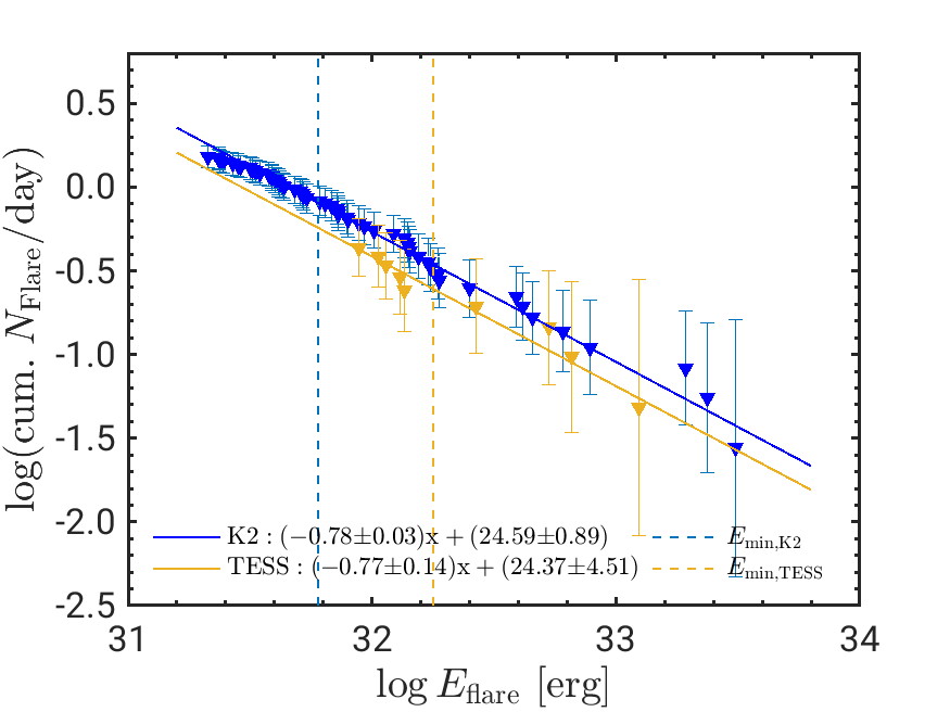
Figure 15: TESS and K2 FFD of TYC 1330-879-1 yielding the same flare rates in both instruments. Only data points above the sensitivity limits $E_{\rm min,th}$, marked by the vertical dashed lines, are considered in both fits. See Sect. 4.6 for the determination of $E_{\rm min,th}$.

5.1.2 From K2 to X-rays

Opportunities to study the relation between flares in white-light and in X-rays have been rare, and the corresponding literature is not abundant. We make here use of two studies with flares observed simultaneously in both wavebands, Guarcello et al. (2019) and Kuznetsov & Kolotkov (2021), in order to establish a calibration between optical and X-ray flare energies.

The work of Guarcello et al. (2019) is based on the simultaneous K2 and XMM-Newton (PI Drake, obs. IDs 0761920-101, -201, -301, -401, -501, -601) observations of the Pleiades cluster. The $12$ brightest flares in this data set have been analyzed by Guarcello et al. (2019) and a relation between the flare energy in the K2 band and in soft X-rays was presented. We used the energy values given in Table 4 of Guarcello et al. (2019). Their flare sample comprises some events on F and G stars. We kept only the $10$ flare events on M-type stars to adapt the sample of stars used for the K2 to X-ray calibration to our M dwarf sample.

We complemented these data with the results of the study of Kuznetsov & Kolotkov (2021) who also studied flares observed simultaneously with Kepler and XMM-Newton. They give flare energies in both bands for nine flare events in their Table 2. For our energy calibration, we excluded one event with a much larger X-ray flare energy than the remaining ones. The three flaring stars analyzed by Kuznetsov & Kolotkov (2021) are of SpT K7, M2, and M3 and have rotation periods of $8.55$ d, $1.50$ d and $6.04$ d, respectively. The SpT of the ten M-type stars in the Guarcello et al. (2019) sample ranges from K8 to M5 and the $P_{\rm rot}$ ranges from $0.22$ d to $4.49$ d. These values are in good agreement with the SpT and $P_{\rm rot}$ range of our sample (cf. Fig. 6).

Fig. 16 shows the X-ray flare energy versus optical flare energy in the Kepler/K2 band for the flare events of the ten M dwarfs in the Guarcello et al. (2019) sample, together with the eight flare events of Kuznetsov & Kolotkov (2021). We fitted a linear relation of the type $y=ax+b$ to these data, where $x=E_{\rm K2}$ is the flare energy in the Kepler/K2 band and $y=E_{\rm X}$ the flare energy in the XMM-Newton X-ray band. We note that Guarcello et al. (2019) and Kuznetsov & Kolotkov (2021) use different XMM-Newton energy bands ($0.3-7.9$ keV versus $0.2-12$ keV). However, given the difference of only $0.1$ keV at the low energy end and the fact that most of the stellar X-rays are emitted at soft energies ($<5$ keV), this is unlikely to affect our analysis.

To minimize the error of the y-axis offset, $b$, we shifted $E_{\rm K2}$ such that the zeropoint of the x-axis lies in the middle between the highest and lowest K2 flare energy of the flares shown in Fig. 16. This way smaller errors of the y-axis offset are achieved. In order to be able to consider uncertainties in both $E_{\rm X}$ and $E_{\rm K2}$ in the fit, we used orthogonal distance regression (ODR). Symmetric uncertainties are required for the fitting, and we took the larger values of the asymmetric errors presented in the literature accepting that this leads to a slight overestimate of the errors. The fit result is also displayed in Fig. 16. The black dashed line marks the 1:1 relation (i.e., $E_{\rm X}=E_{\rm K2}$). As a result of the fit, we obtained

$$\text{log}(E_{\rm X})=(1.42\pm 0.37)\cdot(\text{log}(E_{\rm K2})-33.57)+(33.06\pm 0.12),$$ (5)

where $E_{\rm X}$ and $E_{\rm K2}$ are given in erg.

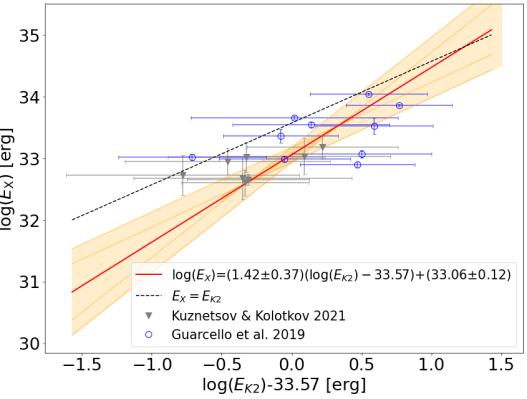
Figure 16: XMM-Newton versus K2 flare energy of the M stars from Guarcello et al. (2019), Table 4 and Kuznetsov & Kolotkov (2021), Table 2. The red line displays a linear fit taking into account uncertainties in both $E_{\rm X}$ and $E_{\rm K2}$. $E_{\rm K2}$ was shifted to minimize the error of the y-axis offset. The orange area comprises fit uncertainties in y-axis offset and slope. See Sect. 5.1.2 for details.

5.1.3 Calibration based on the multiwavelength data

The calibrations presented in Sects. 5.1.1 and 5.1.2 can be combined to estimate for a flare observed with TESS its equivalent energy output in the XMM-Newton X-ray band. As discussed in Sect. 5.1.1, no conversion is necessary between flare energies in the TESS and K2 band. Thus, we obtain the flare energy in the X-ray band by applying the relation obtained from the fit to the Pleiades M-type stars of Guarcello et al. (2019) and the field M-type stars of Kuznetsov & Kolotkov (2021) directly to our TESS flare energies:

$$\text{log}(E_{\rm X})=a\cdot(\text{log}(E_{TESS})-33.57)+b,$$ (6)

with the values of $a=1.42\pm 0.37$ and $b=33.06\pm 0.12$ derived in Sect. 5.1.2 and $E_{\rm X}$ and $E_{\rm K2}$ in units of erg.

The optical/X-ray flares on which we calibrated the relation between $E_{\rm K2}$ and $E_{\rm X}$ comprise flare energies between roughly $10^{32.5}$ erg and $10^{34.5}$ erg. Our calibration between the TESS and K2 FFDs has been derived for slightly lower energies ($\lesssim 10^{33.5}$ erg, cf. Fig. 15). However, no change in power law slope is expected at higher energies. Flare energy frequency distributions with similar slopes to that found by us for TYC 1330-879-1 have been observed on superflare stars with energies up to $10^{36}$ erg (Shibayama et al., 2013). Raetz et al. (2020) studied the FFDs of M dwarfs covering a range of activity levels, which translate into a vertical offset of the FFDs but do not affect the slope. A similar result is seen in the literature compilation of FFDs by Ilin et al. (2019). Therefore, the one-to-one correspondence between TESS and K2 flare frequencies can safely be extrapolated to higher flare energies.

5.2 X-ray FFDs

Figure 17: Average TESS FFDs for stars with reliable $P_{\rm rot}$ in the early (M2.5$-$M3.5) and late (M4.5$-$M5) SpT range derived in Sect. 4.6 (black) and constructed X-ray FFDs based on the energy conversion derived in Sect. 5.1.3 (red). Error bars on $E_{\rm X}$ represent the uncertainty caused by this conversion. Error bars on the flare rate are the same for the observed TESS (black) and constructed XMM-Newton (red) FFDs and result from Eq. 4. The green line represents the extrapolation to small flare energies for the observed X-ray FFD that Getman & Feigelson (2021) found for PMS stars with masses $\leq 1M_{\odot}$. The slopes of our power law fits are given in Table 4.

We can now use the relation between optical and X-ray flare energies derived in Sect. 5.1.3 to construct X-ray FFDs for our HZCat sample directly from the observed TESS flares. We do this separately for the two average TESS FFDs of our early (M2.5$-$M3.5) and late (M4.5$-$M5) samples with reliable rotation period. The X-ray FFDs are obtained by shifting each energy value of the average TESS FFDs from Fig. 13 into the XMM-Newton X-ray band with the relation in Eq. 6. The result is shown in Fig. 17 (red) together with the observed TESS FFDs (black). For comparison, we also show the observed X-ray FFD in the low-mass regime ($\leq 1\,M_{\odot}$) from the pre-MS star study of Getman & Feigelson (2021). We subtracted a constant value of $\log{365.25}$ from the published relation of Getman & Feigelson (2021) since they give flare rates in units of ${\rm yr^{-1}}$.

We performed a linear fit on our constructed X-ray FFDs. In order to be able to consider both the errors in $E_{\rm X}$ resulting from the energy conversion and the flare rate uncertainties, we again used ODR. The resulting FFD power law slopes and their uncertainties, which are the formal errors of the fit, are given in Table 4 together with the power law slopes of our two SpT-averaged TESS FFDs. The synthesized X-ray FFDs are less steep than the observed TESS FFDs because the slope of our $E_{\rm K2}$ to $E_{\rm X}$ calibration (Eq. 5) is steeper than the 1:1 relation. Further, the X-ray FFDs are shifted toward lower flare energies with respect to the optical ones. This directly follows from the fact that almost all flare events used for the calibration show higher energies in the K2 band than in X-rays (cf. Fig. 16).

We note that our transformation from optical to X-ray FFDs involves the assumption of a 1:1 correspondence of the flare occurrence in both calibration steps: from TESS to K2 as well as from K2 to X-rays. There are two aspects about this assumption: first, the actual physical 1:1 correspondence in flare occurrence, and second, the 1:1 correspondence in observations which might be impeded by different detection biases for the two instruments. That each TESS flare is associated with a flare in the K2 band should be fulfilled as they both represent white-light emission. Moreover, we have demonstrated that TESS and K2 yield identical FFDs (see Sect. 5.1.1).

The optical to X-ray calibration is more complex. Regarding the physical 1:1 correspondence in flare occurrence in this case, it is instructive to have a look at results for our Sun. In the standard solar flare picture, optical flares are the result of bombardment of the lower atmosphere with particles accelerated in the corona; the ensuing density enhancement and heating of the corona produces the soft X-ray flare (e.g., Antonucci et al. 1982, Cargill & Priest 1983), which is detected in the case of stellar flares with XMM-Newton. For the case of the Sun there seems not to be an unexpectedly high number of soft X-ray flares without an optical counterpart or vice versa: Milligan & Ireland (2018) systematically studied the number of solar flares greater than GOES C1 class in solar Cycle 24 that were observed simultaneously by instruments operating at different wavelengths. For various combinations of instruments, they compared the actual number of simultaneously observed flares to the number that can be expected theoretically, assuming that the instruments operate independently and considering for each instrument its rate of success to observe a flare. For the Solar Optical Telescope (SOT, Tsuneta et al. 2008), the number of flares captured simultaneously with the X-Ray Telescope of the Hinode mission (XRT, Golub et al. 2007) was higher than the expected value. Since Milligan & Ireland (2018) took into account the detection sensitivity of each instrument, this means that they did not find a discrepancy that could be attributed to an actual lack of counterparts in either of the two bands.

The second caveat in our transformation of optical to X-ray FFDs regards detection biases. Even if each soft X-ray flare comes with an optical counterpart and vice versa, it might happen that one of the two events is not captured by the respective instrument due to sensitivity biases or other circumstances. This means that we are translating any potential bias in TESS flare observations while we are not considering the observation biases in the X-ray band. Apart from the sensitivity of each individual instrument toward flare detection, here the viewing geometry of a flare event may also play a role for its visibility in different bands: For instance, Flaccomio et al. (2018) explained X-ray flares without optical counterpart in the star forming region NGC 2264 by events occurring behind the limb such that the lower-lying optical emission remains hidden to our view while the more extended coronal loops are still partly visible. We note that the majority of their X-ray flares had an optical counterpart, strengthening our hypothesis of each optical flare being associated with an X-ray flare and the other way round.

To summarize, we have constructed X-ray FFDs by translating TESS flare rates from the optical energy at which they have been observed to the calibrated X-ray flare energy. These X-ray FFDs represent a prediction for the FFDs that hypothetical observations of our stars in the XMM-Newton energy band would yield. They are based on strong assumptions, (1) that each optical flare is associated with an X-ray flare and vice versa as discussed in detail above, and (2) that the sensitivity and biases for flare detection are the same for TESS and XMM-Newton. As long as no observational constraints for X-ray FFDs are available our prediction may serve as a useful input to planet irradiation models for active M dwarfs.

6 Discussion

6.1 Optical flares and rotation on HZCat stars

We analyzed the activity and rotation properties of $109$ M dwarfs using TESS LCs. The stars were selected to have the characteristic that planets in their entire HZ can be detected with TESS through their transits. For two of our targets, in fact, TESS has discovered planets that were confirmed by follow-up observations. Two targets have planets discoverd with other methods, and four additional stars within our sample are classified as TOI.

6.1.1 Statistics of rotation period detections

We detected rotation periods on $12$ stars, only $11.0$ % of the sample. This fraction is low compared to numbers found for M dwarfs in Kepler studies, for example McQuillan et al. 2013 ($63.2$ %), Stelzer et al. 2016 ($72.4$ %) or Raetz et al. 2020 ($82.1$ %). One possible reason for the low period detection fraction in our sample is the lower photometric precision of TESS with respect to Kepler and K2 LCs (cf. Fig. 7), which makes the notoriously small amplitudes of spot modulations in M dwarfs difficult to distinguish from the noise. Canto Martins et al. (2020) examined rotation periods of $1000$ TOIs using 2-minute cadence LCs of the first $20$ months of the TESS mission. They found only $131$ targets with unambiguous rotation periods, that is a fraction of $13.1$ %, which is in good agreement with the $11.0$ % for our smaller sample. However, when comparing our results to literature studies, it also has to be considered that our period search is a priori limited to a maximum period of $13.5$ d (cf. Sect. 3.2). McQuillan et al. (2013) find rotation periods below this limit for a fraction of only $7.5$ % of their sample, and thus our value of $11.0$ % is even slightly higher. In the sample of Stelzer et al. (2016), $17.9$ % of the analyzed stars have $P_{\rm rot}<13.5$ d. Medina et al. (2020) searched for rotation periods with TESS photometry and ground based photometry from MEarth using as subsample the volume-complete $15$ pc mid- to late-M dwarf sample of Winters et al. (2021). They included previously published rotation periods from the literature for about $1/4$ of their sample and they found that in their total sample of $125$ stars $27.2$ % have $P_{\rm rot}<13.5$ d. Thus, our fraction of $11$ % of stars with measured $P_{\rm rot}$ from TESS photometry is by at most a factor of two lower than the results from Kepler, K2 or ground-based studies.

6.1.2 Statistics of flare detections

Flares are present on a much larger number of stars than rotation periods ($35$ out of $109$ stars, that is $32.1$ % of the sample). However, $84\,\%$ of the flares we detect are found on the $12$ stars with reliable $P_{\rm rot}$ that are all fast rotators. Raetz et al. (2020) established a bimodality in the flare rate with frequent events on stars with $P_{\rm rot}\lesssim 10$ d and low flare rate for slower rotators. An enhanced flare frequency on fast rotators was also found in other studies, for example Zeldes et al. (2021).

The observed flare rate depends also on the observing cadence and SpT of the sample. Yang & Liu (2019) have presented a flare catalog of the Kepler mission that comprises $3420$ flaring stars. Their flare incidence rate for M stars is significantly lower ($9.74$ %) than our result. We note that their work is based on Kepler long cadence LCs, which is likely the main reason for the lower flare incidence rate. Yang et al. (2018) compared flare properties in long and short cadence LCs of the entire Kepler mission data set and found that a majority ( about $60$ %) of the short cadence flares have no long cadence counterpart. Raetz et al. (2020) found an even lower fraction of $31$ % of short cadence flares recovered in long cadence for their M dwarf sample. Günther et al. (2020) analyzed a large sample of $24809$ stars observed in the first two months of the TESS mission in 2-minute cadence. They found a flare occurrence rate of $>40$% for mid- to late-M stars (SpT M4 to M6) and $10$ % for early-M stars. These numbers are in better agreement with our flare occurrence rate of $32$ % although our sample does not only comprise mid to late-M stars. Günther et al. (2020) also found that M4 to M6 dwarfs show the highest fractions of flaring targets. This is in good agreement with the SpT distribution of the flaring stars in our sample. An increase of the fraction of flaring stars from SpT M0 to M5 was also seen by Yang et al. (2017) and by Lu et al. (2019), both based on Kepler and K2 long-cadence data. Rodríguez Martínez et al. (2020) found the same for LCs of $1376$ nearby M dwarfs from the All-Sky Automated Survey for Supernovae (ASAS-SN, Shappee et al. 2014, Kochanek et al. 2017).

To account for detection biases we calculated flare rates for our sample considering two different detection completeness limits regarding (i) the flare luminosity amplitude (described in Sect. 4.4) and (ii) the flare energy (described in Sect. 4.6). As a universal limit for the minimum flare amplitude required for detection within all stars of our sample we had determined a luminosity amplitude $L_{\rm max,th}$ with a value of $3.4\cdot 10^{29}$ erg/s. The average flare rate over all $109$ stares and considering only flares above $L_{\rm max,th}$ is $0.043\,\rm d^{-1}$ ($1275$ flares on $30$ stars). Considering only the $30$ stars that present events above this critical luminosity amplitude we find $\overline{\nu}_{\rm F,L_{\rm max,th}}\approx 0.168\leavevmode\nobreak\ \textrm{d}^{-1}$. However, we found a strong SpT dependence of the flare rate, with no flares at all detected on stars with SpT earlier than M2.0 and a peak in the flare rate around M3$-$M4.

Similar to $L_{\rm max,th}$ we can define a conservative threshold for the completeness in terms of flare energy from the FFDs. The FFD analysis was carried out only for the $12$ stars with measured rotation period, seven of which have contamination factors $<10$ % and are single stars. This latter subsample comes up for $\sim 50$ % of all detected flares. We take as energy threshold the largest value of the $E_{\rm min,th}$ among all those present in the sample. The rate of all events above this $(\langle E_{\rm min,th}\rangle)_{\rm max}$ averaged over the $7$ stars is $\bar{\nu}_{\rm F,L_{\rm max,th}}=0.682\,\rm d^{-1}$ .

Among the eight known planet host stars and TOIs, only TOI-1450 and L34-26 show flares above the amplitude threshold. The latter is the most active star among the planet hosts and the only one for which we measured a rotation period. It is fast-rotating ($P_{\rm rot}=2.83$ d) and shows flares at a frequency of $0.48$ d^-1 above the detection threshold, $L_{\rm max,th}$. The planet, however, should not be influenced by the host star’s activity, given its large orbital separation (cf. Sect. 4.7).

6.1.3 Relation between flare amplitude and duration

We found a linear relation between flare amplitude and duration for our sample of 2532 flares that is similar to the one determined by Raetz et al. (2020) based on K2 short cadence data (cf. Fig. 11). The slope found by Hawley et al. (2014) for Kepler short cadence observations of the highly active M dwarf GJ 1243 is slightly steeper than what we found for our sample. More drastic is the shift between our amplitude-duration distributions and that of GJ 1243.

Since GJ 1243 has been considered a prototypical flare star it is relevant to examine the characteristics of its events in the context of larger samples of M dwarfs. There are three possible sources for the differences with respect to our amplitude-duration distributions: A possible explanation could be a systematic difference in flare duration measurements between our analysis and that of Hawley et al. (2014). Analogously to our method, Hawley et al. (2014) also measure the flare duration as the time difference between the first and last flare point. In doing so, they determine flare points by visual inspection while we rely on the output of our flare search algorithm. This makes it difficult to draw a conclusion on whether systematic differences in the flare duration measurement are responsible for the different slopes in the amplitude-duration relation. Secondly, the different instruments used could play a role. The higher standard deviation in TESS LCs compared to K2 (cf. Fig. 7) might lead to underestimated flare durations with TESS inasmuch as flare points at the end of the decay phase disappear in the noise. We expect this to have a larger effect on longer flares, simply because they have a longer decay phase. Flare amplitudes should be affected much less by a higher noise level since they are determined as the difference between the peak flare flux and the flux of the smoothed, interpolated LC at the time of the flare peak. A potential understimation of the flare duration would shift the TESS amplitude-duration relation to the left, as observed when we compare our sample to GJ 1243. Finally, GJ 1243 might simply exhibit flares of a certain shape such that the flare amplitude grows faster with the duration.

We further found for our HZCat stars that the relative flare amplitude $A_{\rm peak}$ as a function of the flare duration is indistinguishable for the early and mid/late SpT subsample, whereas the absolute flare amplitude $\Delta L_{\rm F,T}$ is shifted upward for the earlier SpTs (cf. Fig. 11). This is a consequence of their higher quiescent luminosity and ensuing higher detection threshold.

6.1.4 Slope of flare frequency distributions

We have presented a detailed study of cumulative FFDs, which yielded for the $12$ stars with reliable rotation period values from $-1.27$ to $-0.84$ for the power law slopes $\alpha$ from Eq. 3. Converting the differential flare distributions given by Yang et al. (2017) to the cumulative form yields power law slopes of $-1.19\pm 0.33$ for the $15$ M stars within their sample of 540 that have Kepler short cadence data. Similarly, the cumulative power law slope found by Lu et al. (2019) is $-1.02\pm 0.11$ for $K2/Kepler$ long cadence data. Raetz et al. (2020) found slopes ranging from $-0.81$ to $-0.85$ for different M SpT subranges, which is consistent with the result of Lin et al. (2019). These latter authors found a value of $-0.86$ for the $548$ M dwarfs within their sample and a slope of $-0.78$ for a subsample of $375$ fast rotating M dwarfs ($P_{\rm rot}<10$ d) based on K2 long cadence data. We note that a steepening of the FFD at the high-energy end, and therefore a deviation from the single power law shape, has been observed in previous flare studies, e.g., Lurie et al. (2015) and Silverberg et al. (2016). Both these studies are based on data from the Kepler mission. The authors suggest that the steepening of the FFD toward higher flare energies might not be a real feature, but either a result of CCD saturation effects or due to low-number statistics. For the $12$ stars with reliable $P_{\rm rot}$ in our sample, the single power law fits are consistent with the shape of the FFDs at the high-energy end under consideration of flare rate uncertainties. These uncertainties are increasing for high-energy events as only a small number of them is observed for each star. This leads to a blurred shape of the FFD, which makes it difficult to assess the shape of the power law at the highest observed flare energies. With this caveat in mind, our power law slopes for the FFDs are in good agreement with the range spanned by previous studies.

In summary, the consistency of our results with previous literature studies on larger samples shows that the rotation and flare properties of this subsample with HZs accessible for TESS transit detections is representative for the class of M dwarfs.

6.2 From optical to X-ray flares

Given the importance of these stars for planet detections, we went one step further and made some inferences on the expected properties of their X-ray flares. Such events quite inevitably take place on active M dwarfs, and the ionizing high-energy radiation has likely a stronger impact on the evolution of the planet than the lower-energy optical flare photons. However, a similarly detailed study of X-ray flare energy distributions is impossible in the foreseeable future because no X-ray space-mission dedicated to long-term monitoring of a significant number of stars is at the horizon. Therefore, combining the few available data sets in which flares were observed at more than one wavelength is a useful alternative for estimating the X-ray FFD. To this end, we have combined the simultaneous XMM-Newton and K2/Kepler observations of 10 M-type stars in the Pleiades presented by Guarcello et al. (2019) and three field M-type stars from Kuznetsov & Kolotkov (2021) with the simultaneous TESS and K2 observation of a single M dwarf, TYC 1330-879-1, analyzed by us specifically for the scope of transforming observed TESS flare properties to the K2/Kepler band. We found that the FFDs of TESS and the K2 mission map one-to-one to each other, namely the energies of flares seen in the TESS band are equal to the corresponding K2 flare energies. Davenport et al. (2020) also found equivalent TESS and K2 FFDs for the active M4 star GJ1243. Therefore, we can directly use the simultaneous K2/XMM-Newton sample to calibrate optical TESS flare energies to the X-ray band.

Under the assumption of a 1:1 correspondence between the occurrence of optical and X-ray flares, we converted the observed TESS FFDs to synthetic X-ray FFDs. This involves the propagation of eventual biases in TESS flare detection while those in the X-ray band are not considered. Our constructed X-ray FFDs are shifted toward lower flare energies with respect to the observed TESS FFDs in the respective SpT subset (cf. Fig. 17). This is explained by the fact that in our calibration flare sample the energy released in the optical band is larger than that released in the X-ray band. Due to the shortage of simultaneous flare observations for M dwarfs in the optical and X-ray band, our calibration relies on the relatively low number of 18 events. The uncertainty in our $E_{\rm X}$ versus $E_{\rm K2}$ relation allows for a slope of $1$, which results in X-ray FFDs with slopes very similar to those of the observed TESS FFDs. Flaccomio et al. (2018) found for flares of pre-MS stars observed with CoRoT and Chandra a relation between $E_{\rm opt}$ and $E_{\rm X}$ of $E_{\rm opt}=6.37\cdot E_{\rm X}^{0.8}$ (for their reduced major axis fit). This translates to a slope of $1.25$ in the $\log E_{\rm X}$ versus $\log E_{\rm opt}$ relation. Their result is therefore consistent with the slope of our calibration based on the Guarcello et al. (2019) Pleiades M-type stars and the 2021ApJ...912...81K field M stars.

Observational constraints on X-ray flare statistics are not available for M dwarfs to the best of our knowledge. X-ray FFDs have been studied for pre-MS stars (see Getman & Feigelson 2021 and references therein). The completeness limits for the flare energies of these observations are extremely shallow (e.g., $\log{E_{\rm F,min}}\,{\rm[erg]}=36.2$ for the MYStiX/SFiNC sample from Getman & Feigelson (2021) and log $\log{E_{\rm F,min}}\,{\rm[erg]}=35.3$ for the Stelzer et al. (2007) sample in the Taurus and Orion star forming regions.) The slopes of these pre-MS X-ray FFDs are, however, similar to those found from optical FFDs by us and other studies discussed above. If the Getman & Feigelson (2021) results are extrapolated to smaller flare energies, the observed X-ray FFDs lie at $E_{F}\approx 10^{35}$ erg about $1-2$ dex above our predictions (see Fig. 17). Toward lower energies, the difference increases up to about 5 dex at $E_{F}\approx 10^{29}$ erg. One reason might be that we underestimate X-ray flare rates by the direct translation of optical flare rates. This could be caused by a detection bias reducing the number of optical flares observed with respect to their X-ray counterparts. On the Sun, for instance, white-light flares are detected more rarely than soft X-ray flares because of their shorter duration (e.g., Namekata et al. 2017). In any case, flare rates do not come without detection biases and therefore strongly depend on the instrument in use. It is thus likely that different properties of our hypothetical X-ray instrument with relation to Chandra, which is the basis of the Getman & Feigelson (2021) study, influence flare frequencies.

Another possibility to explain this excess in the flare frequency of the pre-MS sample might be the youth of the stars. The X-ray activity level (irrespective of flares) is well known to decrease with stellar age (e.g. Preibisch & Feigelson, 2005; Magaudda et al., 2020). The origin of this “quiescent” X-ray emission is not understood, and unresolved nano-flares are a possible explanation (e.g. Aschwanden et al., 2000). Coffaro et al. (2022) inferred from modeling the X-ray spectra of solar-type stars with observations of our Sun that at an age of $\sim 200$ Myr the whole corona of the star is filled with magnetic structures, and the enhanced X-ray flux of younger stars must be due to increased (unresolved) flaring. Our FFDs apply to the most active of the field M dwarfs (as only fast rotators with clear spot modulation signal were considered) and are certainly in the saturated regime where from inference from solar-type stars, as explained above, part of the X-ray emission should be due to unresolved flaring. Given the negative power law of the FFDs one can expect that resolved flares decay in a similar way throughout stellar evolution as the quiescent (nano-flaring) X-ray luminosity. The discrepancy in the flare rates between our predicted X-ray FFD for active M dwarfs and the observations for pre-MS stars are therefore plausibly explained by the decrease of activity with age. Finally we caution that the “low-mass” sample of Getman & Feigelson (2021) is defined as stars with mass $<1$ $M_{\odot}$, and thus does not represent the young analogs of our stars.

As Ilin et al. (2021) show in their comprehensive summary of published optical stellar FFDs for M dwarfs, different studies have come up with distributions that have vertical offsets of up to two orders of magnitude. Our TESS FFDs would lie at the upper end of these distributions consistent with the high activity of the $12$ stars with reliable $P_{\text{rot}}$ within our sample. One may, therefore, conjecture that the X-ray FFDs of less active M dwarfs are analogously shifted downward to lower frequencies. Future studies of the relation between quiescent X-ray luminosity and X-ray variability, for example with the eROSITA all-sky survey (Predehl et al., 2021), may help to constrain the dependence of the flare rate on the overall level of magnetic activity.

Appendix A Data Tables.

Stellar parameters, TESS contamination factors, rotation periods, flare parameters and observation times for the M dwarf sample. The full tables are available in electronic form at the CDS via anonymous ftp to cdsarc.u-strasbg.fr (130.79.128.5).

Table A.1: Stellar parameters for our $112$ sample stars; see Sect. 2.1 for details.

TIC ID	Other name	Gaia DR2 ID	2MASS ID	RA	Dec	$T$	$M_{*}$	$d$	SpT	log($L_{\textrm{qui},T}$)
				[deg]	[deg]	[mag]	[$M_{\odot}$]	[pc]		[erg/s]
38759628	L 130-37	4677345043203760896	04280568-6209254	67.024	-62.157	10.42	0.331 $\pm$ 0.007	18.241 $\pm$ 0.012	3.5	31.15
55745883	UCAC4 141-004923	4665366619931917824	04593230-6153042	74.885	-61.884	10.17	0.389 $\pm$ 0.008	19.899 $\pm$ 0.01	3.0	31.33
140635646	UCAC4 064-003335	4624560719769978368	04471915-7719483	71.83	-77.33	10.68	0.435 $\pm$ 0.009	32.497 $\pm$ 0.023	1.5	31.55
140998116	UCAC4 066-003833	4624829103685457024	05130604-7653221	78.275	-76.89	10.62	0.341 $\pm$ 0.007	22.157 $\pm$ 0.013	3.0	31.24
$..$	$..$	$..$	$..$	$..$	$..$	$..$	$..$	$..$	$..$	$..$
TIC ID	Other name	Gaia DR2 ID	2MASS ID	RA	Dec	$T$	$M_{*}$	$d$	SpT	log($L_{\textrm{qui},T}$)
				[deg]	[deg]	[mag]	[$M_{\odot}$]	[pc]		[erg/s]

Table A.2: Stellar parameters for CPM pairs.

TIC ID	Gaia DR2 ID	2MASS ID	dist	$G_{RP}$	$R_{*}$	$T_{\textrm{eff}}$	$M_{*}$	SpT	sep.
			[pc]	[mag]	$[R_{\odot}]$	[K]	$[M_{\odot}]$		[′′]
142086812	5260759175761501696	06334337-7537482	8.840$\pm$0.002	8.26	0.425$\pm$0.013	3442$\pm$80	0.443$\pm$0.009	M3V	21.74
142086813	5260759175761502976	06334690-7537301	8.838$\pm$0.003	9.04	0.332$\pm$0.010	3330$\pm$82	0.338$\pm$0.006	M3.5V
149988104	5482312349304478976	06011889-6047092	20.292$\pm$0.020	11.19	0.286$\pm$0.009	3282$\pm$82	0.286$\pm$0.006	M3.5V	6.85
–	5482312418025591808	06011898-6047023	20.371$\pm$0.030	11.78	0.236$\pm$0.007	3194$\pm$81	0.232$\pm$0.005	M4V
$..$	$..$	$..$	$..$	$..$	$..$	$..$	$..$	$..$	$..$

Table A.3: Results of the rotation and flare search and contamination analysis for all stars. Gaps in each LC were subtracted from the observation length (cf. Sect. 4.4).

			contamination factor
TIC ID	observation sectors	obs. duration	mean	min	max	$P_{\text{rot}}$	$N_{\text{flares,tot}}$	$\nu_{\text{flares,thresh}}$
		[d]	[%]	[%]	[%]	[d]	[d]-1	[d]-1
38759628	1-13	302.32	0.6	0.5	0.7	$-$	5	0.003
55745883	1-6;8-13	278.64	2.5	0.0	5.2	$-$	$-$	$-$
140635646	1-9;11-13	281.35	0.4	0.1	0.5	$-$	$-$	$-$
140998116	1-13	304.2	3.8	0.2	9.6	$-$	$-$	$-$
$..$	$..$	$..$	$..$	$..$	$..$	$..$	$..$	$..$

Appendix B Special treatment of the eclipsing binary CM Draconis

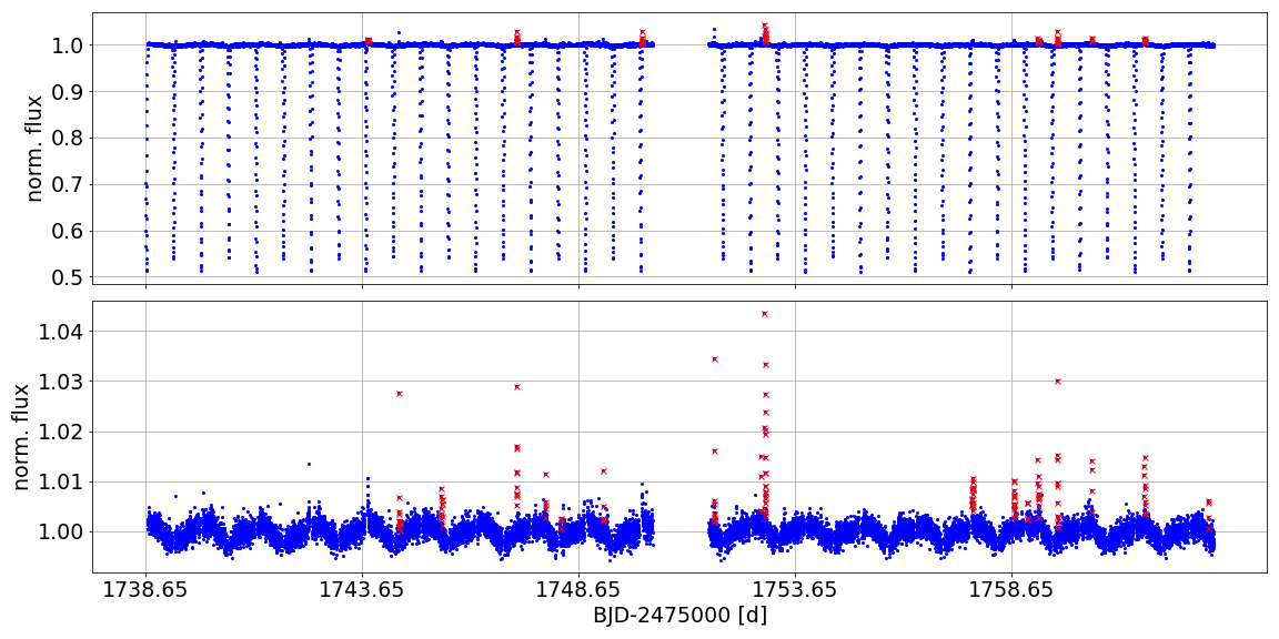
Figure B.1: Top: original LC of the eclipsing binary CM Draconis (TIC 199574208) in sector $16$. Bottom: LC of the same sector after removal of the eclipses as it was used for flare and rotation period search. Validated flares in both panels are marked in red. The rotation period found in the analysis is identical to the orbital period of $1.27$ d, meaning the spin is synchronized to the orbital motion by tidal interaction between the two components. This tidal locking of CM Dra is also reported in the literature (e. g Deeg et al. 1998, Morales et al. 2009).

TIC 199574208 is better known as the eclipsing binary (EB) CM Draconis. The binary system itself comprises two very similar red dwarfs ($M_{1}=0.23M_{\odot}$, $M_{2}=0.21M_{\odot}$) orbiting each other with a period of $T=1.27$ d (e.g., Pribulla et al. 2012). Using the Gaia parallax we estimate a separation of 1.17 mas, and thus the two sources are not resolved by Gaia. The unresolved EB has another companion object: A White Dwarf at a separation of 26.7^′′ sharing the same proper motion that might contaminate the photometry is listed in Table A.2.

The eclipses dominate the LC and make it difficult to analyze other characteristics such as flares or starspot variations. For instance, the eclipses cause a significantly higher standard deviation of the LC and therefore raise the flare detection threshold. Since this work focuses on flare and rotation period search, all data points of the eclipses were removed from all LCs of this star before the final analysis. Fig. B.1 shows as an example in the top panel the original LC of sector $16$ with eclipses and in the bottom panel the LC after removal of the eclipses as it was used for the final analysis. In this sector, the flare search algorithm validated 18 flares in the LC without eclipses while only 8 were found in the original LC.

Appendix C Example LCs of stars with reliable rotation periods

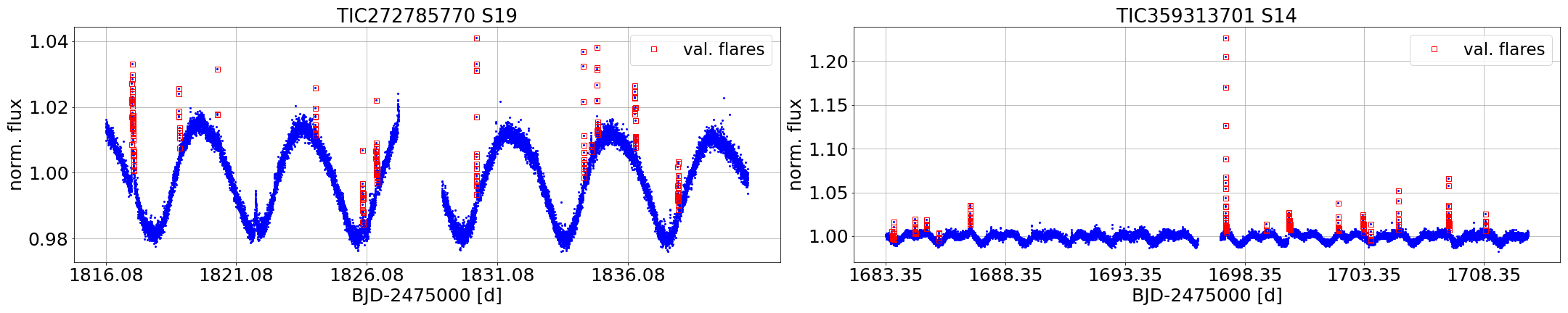
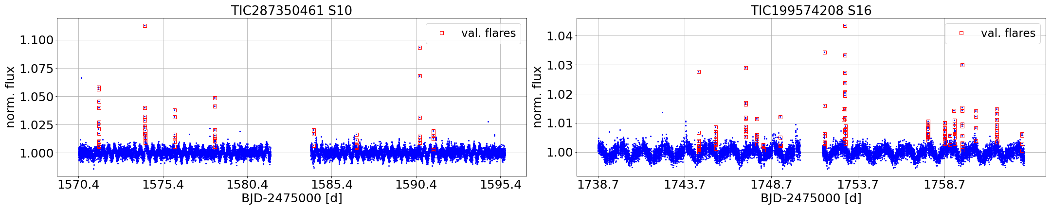
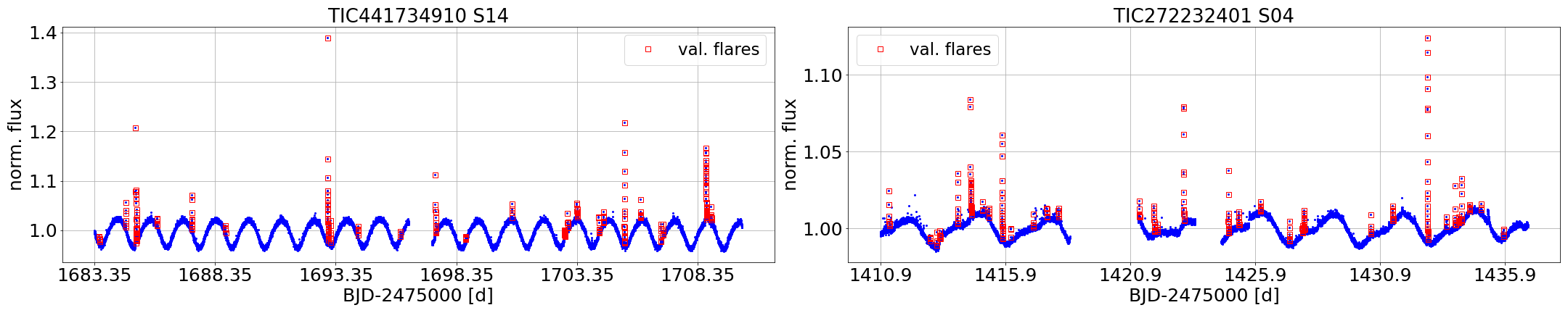
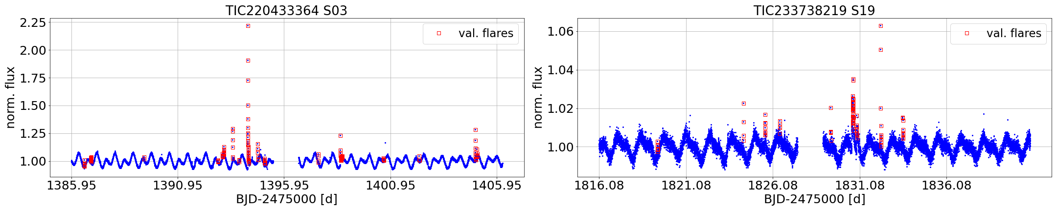
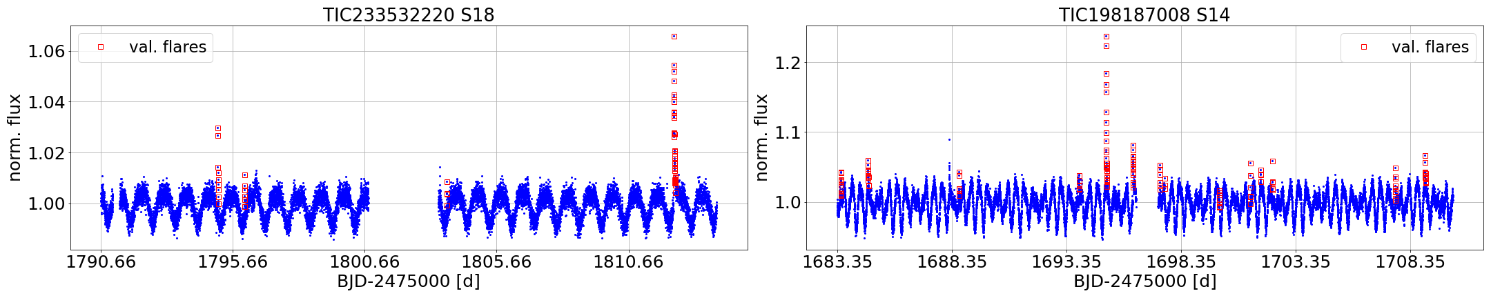
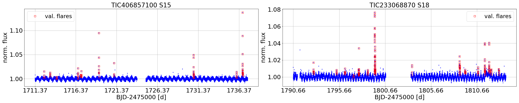
Figure C.1: Examples of TESS LCs; one TESS sector is displayed for each of the $12$ stars with reliable rotation period.

Appendix D Estimating Kepler Magnitudes using Gaia and TESS photometry

Figure D.1: Fit of $K_{p}-T$ vs. $BP-RP$ for about $19000$ nearby main sequence stars.

In order to compare the standard deviations of the flattened LCs ($S_{\text{flat}}$) of the short cadence K2 data from Raetz et al. (2020) to our TESS results (see Sect. 4.3) we had to convert the K2 magnitudes to TESS magnitudes. To this end, we made use of the gaia-kepler.fun crossmatch database created by Megan Bedell. This website provides cross-matched catalogs of Gaia data for stars observed by Kepler/K2. In particular, we downloaded the 1” cross-match of Gaia DR2 (Gaia Collaboration et al. 2018) with the NASA Exoplanet Archive Kepler Stellar Properties Catalog (for Q1-Q17, DR25) consisting of all stellar targets with long-cadence observations from Kepler (Mathur & Huber 2016). This catalog was further matched with Bailer-Jones et al. (2018). The resulting downloaded catalog contains 201312 entries. For our purpose we selected the subsample of 20379 nearby (¡ 500 pc) main-sequence stars (3.8 ¡ log g ¡ 5.2). By using the provided Gaia IDs we cross-matched the catalog with the TESS Input Catalog (TIC v8, Stassun et al. 2018) which results in 19009 entries. This final catalog lists Gaia, Kepler as well as TESS magnitudes.

Fig. D.1 shows the color-color plot using Gaia $BP-RP$ and the difference between Kepler and TESS magnitudes. To estimate the TESS magnitudes of the sample presented by Raetz et al. (2020), we fitted a 7th order polynomial to these data. The result of the fitting is

$$Kp-T=A+Bx+Cx^{2}+Dx^{3}+Ex^{4}+Fx^{5}+Gx^{6}+Hx^{7}$$ (7)

with $x\,=\,BP-RP$ and the coefficients given in Table D.1. By inserting the Gaia color and the K2 magnitude of the R20 sample, we can estimate the TESS magnitude.

Table D.1: Coefficients for the magnitude calibration given in Eq. 7.

Coefficient	Value
$A$	0.0449377231
$B$	0.4603859028
$C$	0.8820614439
$D$	-2.0683447014
$E$	1.8798211314
$F$	-0.8203383843
$G$	0.1721529852
$H$	-0.0139446163

Appendix E FFDs with energy completeness limits for the $12$ stars with reliable rotation periods

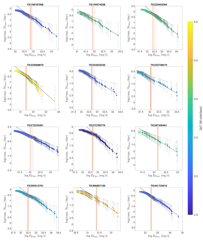
Figure E.1: Cumulative distribution of the flare energies for the $12$ stars with reliable rotation period determined from TESS light curves. The red solid line shows the energy threshold of each TESS sector that we adopted to select the flare events considered in the power law fit.

References

- Allain (1998) Allain, S. 1998, A&A, 333, 629
- Antonucci et al. (1982) Antonucci, E., Gabriel, A. H., Acton, L. W., et al. 1982, Sol. Phys., 78, 107
- Aschwanden et al. (2000) Aschwanden, M. J., Tarbell, T. D., Nightingale, R. W., et al. 2000, ApJ, 535, 1047
- Audard et al. (2000) Audard, M., Güdel, M., Drake, J. J., & Kashyap, V. L. 2000, ApJ, 541, 396