FastLTS: Non-Autoregressive End-to-End Unconstrained Lip-to-Speech Synthesis

Abstract.

Unconstrained lip-to-speech synthesis aims to generate corresponding speeches from silent videos of talking faces with no restriction on head poses or vocabulary. Current works mainly use sequence-to-sequence models to solve this problem, either in an autoregressive architecture or a flow-based non-autoregressive architecture. However, these models suffer from several drawbacks: 1) Instead of directly generating audios, they use a two-stage pipeline that first generates mel-spectrograms and then reconstructs audios from the spectrograms. This causes cumbersome deployment and degradation of speech quality due to error propagation; 2) The audio reconstruction algorithm used by these models limits the inference speed and audio quality, while neural vocoders are not available for these models since their output spectrograms are not accurate enough; 3) The autoregressive model suffers from high inference latency, while the flow-based model has high memory occupancy: neither of them is efficient enough in both time and memory usage. To tackle these problems, we propose FastLTS, a non-autoregressive end-to-end model which can directly synthesize high-quality speech audios from unconstrained talking videos with low latency, and has a relatively small model size. Besides, different from the widely used 3D-CNN visual frontend for lip movement encoding, we for the first time propose a transformer-based visual frontend for this task. Experiments show that our model achieves $19.76\times$ speedup for audio waveform generation compared with the current autoregressive model on input sequences of 3 seconds, and obtains superior audio quality.

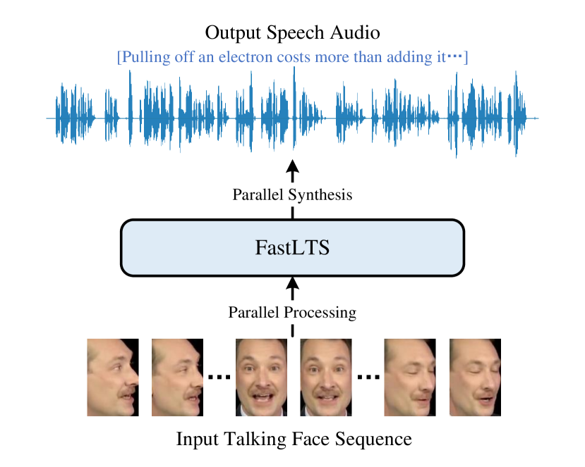
Figure 1. Illustration of end-to-end lip-to-speech synthesis. Corresponding speech audios are generated conditioned on silent talking video frames. Parallel generation is adopted in our non-autoregressive architecture.

teaser

1. Introduction

Lip-to-speech synthesis aims to reconstruct corresponding speech audios from silent videos of talking human faces by analyzing the facial movements, especially the movements of lips. This technology can help people understand speech in situations where voices are hardly audible, such as video conferencing in silent or noisy environment (Vougioukas et al., 2019), long-range listening for surveillance (Ephrat et al., 2017) and so on. Therefore, it has attracted a big attention from researchers.

Most existing methods of lip-to-speech synthesis (Ephrat and Peleg, 2017; Ephrat et al., 2017; Akbari et al., 2018; Vougioukas et al., 2019; Michelsanti et al., 2020; Yadav et al., 2021; Mira et al., 2021; Kim et al., 2021a) focus on constrained settings with small datasets, such as GRID (Cooke et al., 2006) and TCD-TIMIT (Harte and Gillen, 2015), where each speaker’s vocabulary contains less than a hundred words, and the speakers are always facing forward with almost no head movement. On the other hand, unconstrained lip-to-speech synthesis uses real-world talking videos which contain vocabulary of thousands of words and large head movements. This is much more difficult than the constrained settings, and most models for constrained lip-to-speech synthesis fail under the unconstrained settings (Prajwal et al., 2020).

Current works (Prajwal et al., 2020; He et al., 2022) show that the sequence-to-sequence (Sutskever et al., 2014; Cho et al., 2014) architecture is an effective solution to this problem. These works combine a visual encoder consisting of a stack of 3D-CNNs (Tran et al., 2015) and an LSTM (Schuster and Paliwal, 1997) with acoustic models from TTS models (Shen et al., 2018; Ren et al., 2019, 2021), either adopting an autoregressive architecture (Prajwal et al., 2020) or a flow-based non-autoregressive architecture (He et al., 2022). They use a two-stage pipeline that first generates mel-spectrograms as intermediate representations, and then synthesizes audio waveforms from the spectrograms with a signal-processing-based algorithm (i.e. Griffin-Lim algorithm (Griffin and Lim, 1984)). These works outperform previous works by a wide margin under unconstrained settings (Prajwal et al., 2020; He et al., 2022).

Despite the impressive results achieved by these models, their two-stage pipeline design has some notable drawbacks. Such a pipeline increases the deployment cost of the model (Tan et al., 2021; Weiss et al., 2021), and limits the audio quality due to error propagation and information loss in the intermediate representations (Kim et al., 2021b; Donahue et al., 2021). Besides, the audio synthesis algorithm used in the second stage further limits the inference speed and audio quality, as it contains a large amount of serial calculations (Griffin and Lim, 1984), and tends to produce low-quality audios with characteristic artifacts (Shen et al., 2018). Neural vocoders that are widely used in TTS models to synthesis high-quality audios, however, perform poor on these models, since their output spectrograms are not accurate enough for the vocoders to perform well (Prajwal et al., 2020).

In addition, both the autoregressive model (Prajwal et al., 2020) and the flow-based non-autoregressive model (He et al., 2022) suffer from inefficiencies in either inference time or memory usage due to their model characteristics. The autoregressive model suffers from high inference latency due to its recursive nature(Gu et al., 2018; Guo et al., 2019; Ren et al., 2019), while the flow-based model has a large amount of parameters which causes high memory occupancy (see Section 5.6). These drawbacks significantly limit the performance of these models.

In this paper, we propose FastLTS, a non-autoregressive end-to-end model for unconstrained lip-to-speech synthesis. Our model is able to directly synthesize high-quality speeches with much less latency. Specifically, we use a transformer-based non-autoregressive acoustic decoder and a GAN-based vocoder to realize a fully parallelized end-to-end model. We show that our model significantly reduces inference time while improving the audio quality, and has a relatively light model size.

Moreover, transformer architecture has recently achieved equivalent or superior performance to convolutional networks on image and video classification (Dosovitskiy et al., 2021; Arnab et al., 2021; Bertasius et al., 2021), proving its ability of visual feature extraction. However, most lipreading and lip-to-speech synthesis models still use 3D-CNNs for visual feature extraction. A recent work (Serdyuk et al., 2022) shows that a ViT(Dosovitskiy et al., 2021)-based visual frontend outperforms 3D-CNN counterparts in audio-visual automatic speech recognition. However, original ViT calculates self-attention among all tokens from a video, causing huge computation and memory burden, thus is inappropriate for long video sequences.

In this work, we devise a transformer-based visual frontend for visual feature extraction in lip-to-speech synthesis. Experiments show that it has viable feature extracting ability on both large unconstrained datasets and small constrained datasets. As far as we know, this is the first practical transformer-based visual frontend for lip-to-speech synthesis and lipreading.

To conclude, our key contributions are as follows:

• We propose an end-to-end model for unconstrained lip-to-speech synthesis, which is able to synthesize high-quality speeches with much less inference latency.

• We propose a transformer-based visual frontend for lip movement encoding, which shows good performance on both large and small datasets.

• Experiments show that our model achieves $9.14\times$ speedup for mel-spectrogram generation and $19.76\times$ speedup for audio waveform generation compared with the autoregressive model on input sequences of 3 seconds, and obtains superior audio quality.

2. Related Works

2.1. Constrained Lip-to-Speech Synthesis

Constrained lip-to-speech synthesis aims to generate speech audios from silent talking videos where the vocabulary is narrow and the speakers’ heads have almost no movement. Ephrat et al. (Ephrat and Peleg, 2017) propose the first solution to this problem, which uses CNN to predict LPC (Linear Predictive Coding) features from silent talking videos. Later they augment their model to a two-tower CNN-based encoder-decoder model (Ephrat et al., 2017) and encode raw frames and optical flows respectively. Akbari et al. (Akbari et al., 2018) combine an autoencoder that extracts bottleneck features from audio spectrograms with a lipreading network for visual feature extracting. Yadav et al. (Yadav et al., 2021) use stochastic modeling approach with a variational autoencoder. Vougiouskas et al. (Vougioukas et al., 2019) and Mira et al. (Mira et al., 2021) use GAN to directly synthesize audio waveform from video frames. Kim et al. (Kim et al., 2021a) combine GAN with attention mechanism for generating better mel-spectrograms.

Although these works show impressive results on small constrained datasets, they fail to handle unconstrained datasets with large head movements and large vocabulary, which limits their applications in real-world scenarios. Different from these models, our model mainly focuses on unconstrained lip-to-speech synthesis. Yet we also conduct experiments on GRID (Cooke et al., 2006) dataset to prove the modeling ability on small constrained datasets of our model.

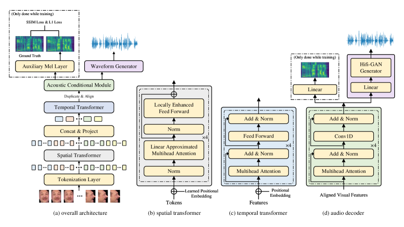
Figure 2. (a) The overall architecture of the model (b) The spatial transformer block (c) The temporal transformer block (d) The audio decoder including the acoustic conditional module and the waveform generator.

architecture

2.2. Unconstrained Lip-to-Speech Synthesis

Unconstrained lip-to-speech synthesis aims to generate speeches from real-world talking videos with large vocabulary and head movements. As this topic has only recently attracted attention of the researchers, there are not many works on it currently. Prajwal et al. (Prajwal et al., 2020) firstly propose an autoregressive sequence-to-sequence model modified from Tacotron 2 (Shen et al., 2018) to tackle this problem, which generates mel-spectrograms conditioned on video frames; He et al. (He et al., 2022) use a non-autoregressive architecture to accelerate inference and use a Glow (Kingma and Dhariwal, 2018) module for mel-spectrogram refinement.

While these models find feasible solution to unconstrained lip-to-speech synthesis, their two-stage pipeline using Griffin-Lim algorithm limits the audio quality and inference speed. Besides, they suffer from low temporal or spatial efficiency due to their model characteristics. Different from these models, our model uses an end-to-end non-autoregressive architecture, which is efficient on both inference time and model size, and also improves the audio quality.

2.3. Vision Transformers

Transformer (Vaswani et al., 2017) has shown decent performance in multiple NLP tasks since it was proposed. Dosovitskiy et al. (Dosovitskiy et al., 2021) bring transformer to the area of computer vision for the first time, and demonstrate that transformer architecture has comparable or even superior performance to convolutional networks on image classification. Later, transformer architecture is extended to videos. Arnab et al. (Arnab et al., 2021) propose a spatial-temporal factorized transformer encoder architecture for video encoding. Several other works (Neimark et al., 2021; Bertasius et al., 2021; Sharir et al., 2021) investigate different attention mechanism for video processing. On the other hand, some works add convolution mechanism to transformers, combining the advantages of convolution and attention mechanism. Wu et al. (Wu et al., 2021) use convolutional networks to calculate self-attention. Yuan et al. (Yuan et al., 2021) add convolution to tokenization layer and feed forward network. Inspired by these works, we propose a spatial-temporal factorized transformer visual encoder for lip-to-speech synthesis. Experiments show that the proposed frontend has comparable encoding ability to traditional convolution networks.

3. Problem Definition

In this section, we introduce the problem formulation of unconstrained lip-to-speech synthesis. Suppose we have a video sequence of a single talking human $V=\{v_{1},v_{2},...,v_{T}\}$, where $T$ denotes the length of the video sequence and $v_{i}$ denotes the i-th frame. The task of lip-to-speech synthesis is to generate the corresponding speech audio $A=\{a_{1},a_{2},...,a_{L}\}$, where $L$ denotes the length of the generated audio, and $a_{j}$ denotes the $j$-th value of the waveform. The relationship between $T$ and $L$ is

(1) $$T\cdot{sr}=L\cdot{FPS}$$

where $sr$ is the sampling rate of the audio and ${FPS}$ is the frame rate of the video.

The word ”unconstrained” means that the head positions of two frames $v_{i}$ and $v_{j}$ may have a big difference where $i$ and $j$ are not very close, and the corresponding speech can have a vocabulary of thousands of words. Constrained lip-to-speech synthesis can be seen as a special case of the unconstrained one.

4. Methods

In this section, we illustrate the architecture of FastLTS and introduce our training methods. As shown in Figure 2(a), the model mainly consists of three parts: the visual encoder (from the tokenization layer to the temporal transformer), the acoustic conditional module, and the waveform generator. A linear layer is used for auxiliary mel-spectrogram output while training. The input video frames are fed into the tokenization layer, then the features are feed forward through the whole model, and finally taken by the waveform generator to synthesize waveforms. We will introduce these modules in detail in the following subsections.

4.1. Visual Encoder

The visual encoder is used to extract and encode visual features from the input video sequence. It consists of a tokenization layer, a spatial transformer and a temporal transformer. The tokenization layer is used to preliminarily extract local features and produce spatio-temporal tokens for the transformer. It consists of a 3D-convolutional layer, a layer normalization layer and a max-pooling layer. The tokens are added with a learned positional embedding and are then fed into the spatial transformer, the architecture of which is illustrated in Figure 2(b). The spatial transformer is used to model the correlation among spatially adjacent tokens, and only calculates attentions on tokens extracted from the same temporal index. However, since the tokens are overlapped while doing tokenization, tokens of the same temporal position may still form a relatively long sequence, causing large computation burden and memory usage. To deal with this problem, we use linear approximation of self-attention proposed in Performer (Choromanski et al., 2021), which significantly reduces the computation burden of self-attention while keeping a good performance. For the feed forward part of the spatial transformer, we employ the Locally Enhanced Feed Forward network proposed in (Yuan et al., 2021), which does convolution on the depth dimension of the features. This brings convolution into the transformer architecture, which strengthens its locality and gives it stronger ability to model spatial correlation among neighboring tokens.

The output hiddens of the spatial transformer with the same temporal index are then concatenated and projected to a single hidden of lower dimension by a linear layer. This sequence is then fed into the temporal transformer, which is illustrated in Figure 2(c). The temporal transformer models the temporal correlation between the hiddens. Its structure is the same as the original transformer proposed in (Vaswani et al., 2017).

4.2. Acoustic Conditional Module

We notice that it is very difficult to directly use audio waveforms as supervisory signal to train the model due to its high dimensionality. Therefore, we employ an acoustic conditional module, which is illustrated in the green part of Figure 2(d). This module works as a non-autoregressive decoder that turns visual features into acoustic features. Basically it is a transformer which alternates the feed forward network with a 1D convolutional network for better locality modeling of the acoustic features. It can output mel-spectrograms when combined with the auxiliary mel layer. Note that this module does not feed mel-spectrograms into the waveform generator, and the auxiliary mel layer is only used to assist training. We will explain the training methods in detail later.

Note that before the output visual features of the temporal transformer are fed into the acoustic conditional module, they need to be aligned to match the length of the acoustic feature sequence. We simply duplicate the visual features for alignment. We calculate the duplication factor $d$ with the formula $d=L_{aud}/FPS$, where $L_{aud}$ is the length of the audio feature sequence per second. If $d$ is an integer, we simply duplicate the visual features by $d$ times. Otherwise, we divide the visual features into two parts and duplicate them by $\lfloor d\rfloor$ and $\lceil d\rceil$ times respectively, and adjust the proportion of the two parts for alignment. For example, if the frame rate is 30 fps and the length of the audio features is 80 per second, we use duplication factors of $\{3,3,2,3,3,2,...\}$.

4.3. Waveform Generator

The structure of the waveform generator is illustrated in the violet part of Figure 2(d). The linear layer has the same dimension as the auxiliary mel layer, and it projects the acoustic features to the same dimension as the mel-spectrogram frame, which is 80 in our case. We then feed the projected features to the generator to synthesize audio waveform. The structure of the generator is the same as that proposed in (Kong et al., 2020). We refer the readers to the Hifi-GAN paper (Kong et al., 2020) for more details about the generator.

4.4. Training Method

As mentioned in section 4.2, due to the high dimensionality of the raw audio, it is very difficult to directly use it as supervisory signal to train the whole model in an end-to-end way. We therefore adopt a two-stage training method. In the first stage, we don’t involve the waveform generator in training, and only train the visual encoder and the acoustic conditional module. We use the auxiliary mel layer to output mel-spectrograms and use SSIM loss (Zhao et al., 2017) and L1 loss to optimize the encoder and the conditional module. The SSIM loss is formulated as:

(2) $$\mathcal{L}_{\rm{SSIM}}=\frac{1}{L_{mel}}\sum_{n=1}^{L_{mel}}1-{\rm SSIM}(y_{n},\hat{y}_{n})$$

Where $L_{mel}$ denotes the length of the mel-spectorgram, $y_{n}$ denotes the $n$-th frame of ground truth mel-spectrogram, $\hat{y}_{n}$ denotes the $n$-th frame of generated mel-spectrogram, and $\rm SSIM(\cdot,\cdot)$ denotes the structural similarity index (Wang et al., 2004) of two vectors. The L1 loss is formulated as:

(3) $$\mathcal{L}_{L1}=\frac{1}{L_{mel}}\sum_{n=1}^{L_{mel}}\lVert y_{n}-\hat{y}_{n}\rVert_{1}$$

And the total loss function of the first stage is:

(4) $$\mathcal{L}_{stage1}=\lambda_{\rm SSIM}\mathcal{L}_{{\rm SSIM}}+\lambda_{L1}\mathcal{L}_{L1}$$

In the second stage, we remove the auxiliary mel-spectrogram output, and plug the waveform generator into the model. We use the same loss as (Kong et al., 2020) to train the whole model. Specifically, we use a multi-period discriminator and a multi-scale discriminator to extract feature maps of the audios and discriminate the audio samples for adversarial training. The training objective of the second stage consists of three parts: adversarial loss, mel-spectrogram loss and feature matching loss. The adversarial loss for discriminators $D$ and generator $G$ is:

(5) $$\mathcal{L}_{adv}(D;G)=\mathbb{E}_{(x,s)}\bigg{[}(D(x)-1)^{2}+(D(G(s)))^{2}\bigg{]}$$

(6) $$\mathcal{L}_{adv}(G;D)=\mathbb{E}_{(x,s)}\bigg{[}(D(G(s))-1)^{2}\bigg{]}$$

Where $s$ is the input condition and $x$ is the ground truth audio.

The mel-spectrogram loss is defined as:

(7) $$\mathcal{L}_{mel}(G)=\mathbb{E}_{(x,s)}\bigg{[}\lVert\phi(x)-\phi(G(s))\rVert_{1}\bigg{]}$$

where $\phi(\cdot)$ denotes the function to transform a waveform into corresponding mel-spectrogram. And the feature matching loss is defined as:

(8) $$\mathcal{L}_{FM}(G;D)=\mathbb{E}_{(x,s)}\left[\sum_{i=1}^{T}\frac{1}{N_{i}}\left\|D^{i}(x)-D^{i}(G(s))\right\|_{1}\right]$$

where $T$ denotes the number of layers in the discriminator; $D^{i}$ and $N^{i}$ denote the features and the number of features in the $i$-th layer of the discriminator, respectively.

The total loss of the second stage is:

(9) $$\mathcal{L}_{stage2-G}=\lambda_{a}\mathcal{L}_{adv}(G;D)+\lambda_{m}\mathcal{L}_{mel}(G)+\lambda_{f}\mathcal{L}_{FM}(G;D)$$

(10) $$\mathcal{L}_{stage2-D}=\mathcal{L}_{adv}(D;G)$$

We find that calculating loss on a whole segment of audio leads to large computation cost and memory usage due to the high resolution of audio. Therefore, we adopt the sampling window technique for wave generator training. Specifically, we sample a consecutive sub-sequence from the acoustic conditional module output, and use the corresponding audio segment to train the waveform generator. We notice that for small dataset, this will reduce computation cost and memory occupancy while keeping a good performance. However, for large unconstrained dataset, training the whole model in this way will damage the encoding ability of the visual encoder due to the shrink of context window. Therefore, we freeze the parameters of the visual encoder and the acoustic conditional module in the second stage and only optimize the parameters of the waveform generator.

5. Experiments and Results

5.1. Datasets

Lip2Wav The Lip2Wav dataset (Prajwal et al., 2020) is the largest and most commonly used dataset for unconstrained lip-to-speech synthesis. It contains real-world lecture videos of 5 different speakers, with about 20 hours of videos per speaker and vocabulary size over 5000 words for each of them. We conduct our experiments on 3 speakers, which are Chess Analysis, Chemistry Lectures and Hardware Security. All three speakers has frame rate of 30 fps, and we sample the raw audios at 16000Hz. We use the same train-test splits as (Prajwal et al., 2020) for training and evaluation.

GRID The GRID dataset (Cooke et al., 2006) is a symbolic dataset for constrained lip-to-speech synthesis. It contains 34 speakers with 1000 sentences uttered by each speaker. The talking videos are captured in an artificial environment. The vocabulary of GRID contains only 51 words. All the sentences are in a restricted grammar and each sentence contains 6 to 10 words. We conduct our experiments on three speakers in the GRID dataset to prove the adaptability on small constrained datasets of our model.

5.2. Implementation Details

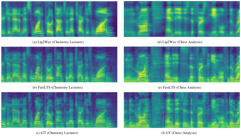
Figure 3. Comparison of mel-spectrograms from different methods

architecture

Data Preprocessing. We use 3-second contiguous sequences as training samples. For audios, we sample the audios at 16000Hz, and transform them to mel-spectrograms with window-size being 800, hop-size being 200 and spectrogram dimension being 80. For video frames, we use $S^{3}FD$ face detector to detect the faces and crop them out. We then resize the cropped faces to $96\times 96$. We use data augmentation for the GRID dataset to improve performance and avoid overfitting. Specifically, we flip the facial images horizontally with probability of 40%, and we randomly crop 0-7.2% horizontal or vertical pixels of the images with probability of 40%.

Model Configurations. The kernel size of the 3D-convolutional layer in the tokenization layer is set to $5\times 5\times 5$. The dimension of the visual tokens $d_{token}$ is set to 32. The spatial transformer is a 4-layer transformer with hidden dimension $d_{s}$ being 36, number of heads $h_{s}$ being 6. The temporal transformer is also a 4-layer transformer with number of heads $h_{t}$ being 8. We set the temporal hidden dimension $d_{t}$ to 384 for the Lip2Wav dataset, and 160 for the GRID dataset. The output dimension of the feed forward layer $d_{ff}$ is $4\times d_{t}$. The acoustic conditional module has the same dimension of hiddens and number of layers as the temporal transformer. For the waveform generator, the kernel sizes of the transposed convolutions $k_{u}$ and the resblocks $k_{r}$ are set to $[9,9,8,4]$ and $[3,7,11]$. The sampling window size is set to 1.2 seconds. For the two training stage, we use Adam and AdamW optimizers, and the initial learning rates are set to $2\times 10^{-3}$ and $2\times 10^{-4}$, respectively.

Table 1. MOS on Lip2Wav Dataset

Speaker	Method	Quality	Intelli.	Natural.
Chess Analysis	Lip2Wav	$3.53\pm 0.10$	$3.51\pm 0.09$	$3.48\pm 0.09$
	FastLTS	$3.79\pm 0.09$	$3.82\pm 0.10$	$3.59\pm 0.08$
	GT	$4.08\pm 0.07$	$3.91\pm 0.08$	$4.10\pm 0.06$
Chemistry Lectures	Lip2Wav	$3.60\pm 0.10$	$3.88\pm 0.10$	$3.78\pm 0.09$
	FastLTS	$3.84\pm 0.10$	$3.73\pm 0.11$	$3.87\pm 0.09$
	GT	$4.06\pm 0.08$	$3.90\pm 0.09$	$4.10\pm 0.07$
Hardware Security	Lip2Wav	$3.67\pm 0.10$	$3.57\pm 0.11$	$3.74\pm 0.11$
	FastLTS	$3.86\pm 0.12$	$3.89\pm 0.13$	$3.80\pm 0.14$
	GT	$3.94\pm 0.10$	$4.01\pm 0.10$	$4.02\pm 0.09$

Table 2. MOS of Lip2Wav + Vocoder ( Failed Cases )

Speaker	Quality	Intelligibility	Naturalness
Chess Analysis	$1.35\pm 0.05$	$1.81\pm 0.04$	$1.54\pm 0.06$
Chemistry Lectures	$1.89\pm 0.04$	$1.47\pm 0.06$	$1.91\pm 0.03$

5.3. Evaluation Metrics

We mainly evaluate the generated audios through subjective evaluation on the quality, intelligibility and naturalness of the audios. Here, quality indicates the clarity of audio against electronic noise and distortion, naturalness indicates how much the prosody and rhythm of the speech sound like real human, and intelligibility indicates the clarity of the pronunciation and the difficulty of understanding the speech content. Our subjective evaluation is conducted via Amazon Mechanical Turk. For each test item, we ask over 300 respondents to fill out three 1-5 Likert scales on the above three metrics of the generated and ground truth audios and report the mean opinion score (MOS). We paid the respondents around $7.2 hourly. We also calculate PESQ (Rix et al., 2001) of our results on the GRID dataset for objective quality evaluation. For inference speed evaluation, we measure the inference speed of mel-spectrograms and waveforms of different models on input sequences of different lengths.

Different from previous works, we don’t calculate STOI (Taal et al., 2011) and ESTOI (Jensen and Taal, 2016) to measure the audio intelligibility, as we claim that these criteria are not appropriate for GAN-based models that directly synthesize audio waveforms. These algorithms measure the distortion of a noisy signal relative to the original one, while GANs may produce intelligible speeches with different intonation from the original speeches, which causes a relatively poor STOI value yet does no damage to intelligibility and naturalness. We therefore mainly use human evaluation for intelligibility evaluation. Later we will release demonstration videos to prove our results.

5.4. Audio Quality

For the Lip2Wav dataset, we conduct human evaluation on the results of FastLTS and Lip2Wav together with the ground truth audios, and present the MOS in Table 1, including mean scores and confidence intervals with confidence level of 95%. We can see that our model achieves significant improvement on audio quality, and improves the speech intelligibility a lot on two speakers. This proves that through adopting an end-to-end architecture with a vocoder, our model is able to generate clearer audios with less noise and distortion, and makes the pronunciation more accurate. Our model also achieves higher score on naturalness, which indicates that it is able to generate more human-like voices with the assistance of adversarial training. The above experimental results also indicate that our transformer-based visual frontend has comparable performance to the 3D-CNN counterparts used in previous works.

We visualize the mel-spectrogram samples generated by different methods in Figure 3 in order to show the superiority of our model more intuitively. We transform the outputs of FastLTS and ground truth audios to mel-spectrograms and compare them with the outputs of Lip2Wav. The left column shows results on speaker of Chemistry Lectures, and the right column shows those on speaker of Chess Analysis. We can see that the spectrograms generated by Lip2Wav tend to be blurry and over-smoothed, while the spectrograms from our model have clear and sharp edges. We marked some areas with red boxes, where the results of the two methods form a striking contrast.

Table 3. MOS on GRID Dataset

Method	Quality	Intelligibility	Naturalness
Lip2Wav	$3.27\pm 0.11$	$3.47\pm 0.13$	$3.54\pm 0.12$
FastLTS	$3.59\pm 0.09$	$3.68\pm 0.09$	$3.73\pm 0.08$
GT	$3.60\pm 0.10$	$3.76\pm 0.09$	$3.78\pm 0.10$

Table 4. PESQ on GRID dataset

Method	PESQ
Vid2Speech (Ephrat and Peleg, 2017)	1.734
Lip2AudSpec (Akbari et al., 2018)	1.673
GAN-based (Vougioukas et al., 2019)	1.684
Ephrat et al. (Ephrat et al., 2017)	1.825
Lip2Wav (Prajwal et al., 2020)	1.772
VAE-based (Yadav et al., 2021)	1.932
Vocoder-based (Michelsanti et al., 2020)	1.900
VCA-GAN (Kim et al., 2021a)	2.008
FastLTS	1.939

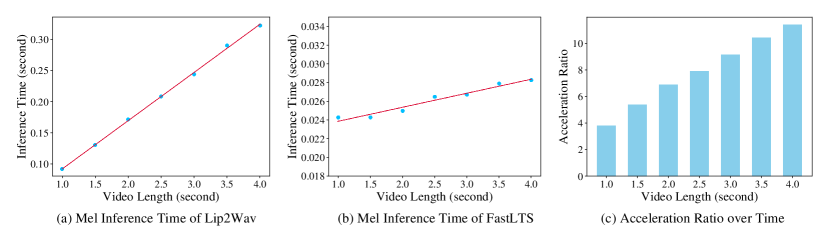
Figure 4. The Inference Speed of Mel-spectrogram of the Two Models

figure description

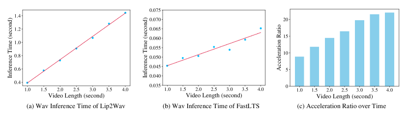
Figure 5. The Inference Speed of Waveform of the Two Models

figure description

We also try to combine the Lip2Wav model with neural vocoders, and report the MOS in Table 2. We train hifi-gan vocoders on the audios and spectrograms from the Lip2Wav dataset, and use them to generate speech waveforms from spectrograms generated by Lip2Wav. We get highly distorted speeches with a strong and harsh electronic noise. As shown in Table 2, these audio samples get extremely low MOS, indicating their low quality. This matches the observation of (Prajwal et al., 2020), and proves that our model is much more than simply adding an acoustic model with a neural vocoder. Our model enables the usage of neural vocoder in unconstrained lip-to-speech synthesis, which is not possible for previous works.

For the GRID dataset, we conduct experiments on three speakers and report the MOS in Table 3. It can be seen that our model achieves a comprehensive improvement on all three aspects, which is consistent with the results under unconstrained settings. We also calculate PESQ and compare our results with the scores of previous works in Table 4. Despite the gap between the results of our model and the state-of-the-art method, our model has outstanding performance and ranks high on the list.

5.5. Inference Speedup

We measure the inference speedup by comparing the inference time of the autoregressive model and our FastLTS model on input video sequences of different lengths. We use the Chemistry Lectures speaker in the Lip2Wav dataset to do the comparison. We conduct our experiments on a server with an Intel-Xeon E5-2678 CPU and an NVIDIA RTX-2080Ti GPU with batch size of 1.

Generally, we don’t directly use the mel-spectrogram output of FastLTS, as it is only used to assist training. Yet we still compare the mel-spectorgram inference speed of the two models to eliminate the effects of using different waveform synthesis methods. The inference time and acceleration ratio are illustrated in Figure 4. We can see that our model generates mel-spectrograms several times faster than Lip2Wav, and the acceleration ratio increases as the input sequence gets longer. This is because our non-autoregressive model adopts parallel generation, so the inference latency doesn’t increase dramatically as the input sequence gets longer, while the latency of Lip2Wav increases sharply due to its autoregressive nature. We can see that the acceleration ratio reaches $9.14\times$ when the input length is 3 seconds which is the configured input length in FastLTS and Lip2Wav.

The waveform inference time of the two models is illustrated in Figure 5. We can see that the Griffin-Lim algorithm causes great inference latency in Lip2Wav, and the latency grows sharply as the mel-spectrogram sequence gets longer, while our model adopts parallel generation of audio with a GAN-based vocoder, which brings great generation speedup. The acceleration ratio of waveform synthesis reaches $19.76\times$ when the input length is 3 seconds. It is worth noting that the acceleration ratio of our model exceeds that of GlowLTS (He et al., 2022). As reported in (He et al., 2022), GlowLTS only achieves $5.337\times$ acceleration when the video length is 30 seconds, and is slower than the autoregressive model when the input length is shorter than 3 seconds.

Table 5. Parameter Amounts of Three Different Models

Model	Parameters	Relative Size
Autoregressive Model
Lip2Wav	39.87M	$1.00\times$
Non-autoregressive Models
GlowLTS	85.92M	$2.16\times$
FastLTS(ours)	50.09M	$1.26\times$

Table 6. CMOS Comparison in Ablation Studies

Method	Quality	Intelli.	Natural.
FastLTS	0	0	0
w/o waveform generator	-0.274	-0.075	-0.103
w/o conditional module	N/A	N/A	N/A
w/o first training stage	N/A	N/A	N/A

5.6. Model Size

We compare the model size of our FastLTS with Lip2Wav and GlowLTS, and the results are shown in Table 5. We can see that as the cost of realizing a non-autoregressive architecture with generative flow, GlowLTS has over twice more parameters than Lip2Wav, causing high memory usage. In contrast, our model only use 26% more parameters to realize an end-to end non-autoregressive architecture that can generate high-quality audio with short latency.

6. Ablation Study

In this section, we conduct ablation experiments on FastLTS to explore the effectiveness of our model. We first remove the waveform generator and conduct CMOS evaluation on the results. The scores are shown in Table 6. We can see that the removal of the waveform generator causes drop in all three aspects, especially the audio quality, where the CMOS is -0.274. This proves that the waveform generator plays an important role in improving the quality, intelligibility and naturalness of the audio. We also visualize the mel-spectrogram samples in Figure 6. It can be seen that the acoustic conditional module tends to generate blurry and over-smoothed spectrograms just like Lip2Wav when there is no waveform generator.

We then remove the acoustic conditional module and try to use raw waveforms to train the whole model. However, we fail to generate intelligible audios with this model. This indicates that the acoustic conditional module plays a significant role in modeling the acoustic features. By comparing the shape of the spectrograms in Figure 6(a) and 6(b), we can infer that acoustic conditional module is responsible for modeling the low-level structures of the audio, while the waveform generator is responsible for complementing high-dimensional details.

We also try to remove the first training stage and train the whole model in an end-to-end way from scratch. All we get, however, are blurry and indistinguishable human voices. This indicates that it is not practical to directly use the raw audio as supervisory signal to train the model, and proves the necessity of the two-stage training.

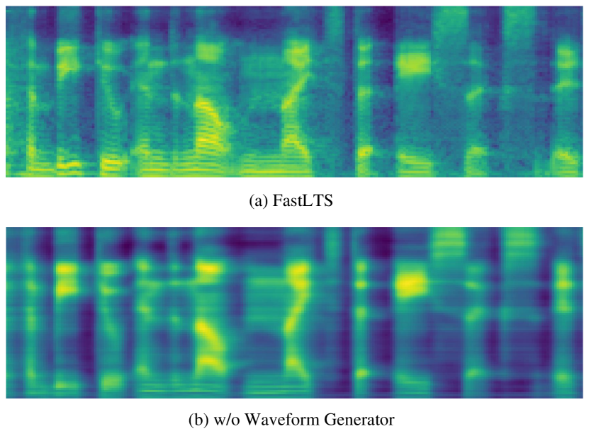
Figure 6. Comparison of mel-spectrograms for ablation studies

figure description

7. Conclusions

In this paper, we devise FastLTS, an end-to-end model for unconstrained lip-to-speech synthesis. To improve audio quality, we build an end-to-end model by using a GAN-based vocoder and applying adversarial training. To reduce inference latency, we adopt a fully parallelized architecture with a non-autoregressive decoder and the vocoder. Besides, we design an applicable transformer-based visual frontend for this task, which shows equivalent performance to 3D-CNN-based counterparts. We conduct experiments on the Lip2Wav dataset, showing significant improvements on audio quality and inference speed. We also conduct experiments on the GRID dataset, showing the adaptability of our model on small datasets.

For future work, we will try to extend the model to multi-speaker settings. We also plan to combine our lip-to-speech synthesis model with human-face super-resolution models to tackle the problem of lip-to-speech synthesis with low-resolution videos.

- (1)
- Akbari et al. (2018) Hassan Akbari, Himani Arora, Liangliang Cao, and Nima Mesgarani. 2018. Lip2Audspec: Speech Reconstruction from Silent Lip Movements Video. In 2018 IEEE International Conference on Acoustics, Speech and Signal Processing, ICASSP 2018, Calgary, AB, Canada, April 15-20, 2018. IEEE, 2516–2520. https://doi.org/10.1109/ICASSP.2018.8461856
- Arnab et al. (2021) Anurag Arnab, Mostafa Dehghani, Georg Heigold, Chen Sun, Mario Lucic, and Cordelia Schmid. 2021. ViViT: A Video Vision Transformer. In 2021 IEEE/CVF International Conference on Computer Vision, ICCV 2021, Montreal, QC, Canada, October 10-17, 2021. IEEE, 6816–6826. https://doi.org/10.1109/ICCV48922.2021.00676
- Bertasius et al. (2021) Gedas Bertasius, Heng Wang, and Lorenzo Torresani. 2021. Is Space-Time Attention All You Need for Video Understanding?. In Proceedings of the 38th International Conference on Machine Learning, ICML 2021, 18-24 July 2021, Virtual Event (Proceedings of Machine Learning Research, Vol. 139), Marina Meila and Tong Zhang (Eds.). PMLR, 813–824. http://proceedings.mlr.press/v139/bertasius21a.html
- Cho et al. (2014) Kyunghyun Cho, Bart van Merrienboer, Dzmitry Bahdanau, and Yoshua Bengio. 2014. On the Properties of Neural Machine Translation: Encoder-Decoder Approaches. In Proceedings of SSST@EMNLP 2014, Eighth Workshop on Syntax, Semantics and Structure in Statistical Translation, Doha, Qatar, 25 October 2014, Dekai Wu, Marine Carpuat, Xavier Carreras, and Eva Maria Vecchi (Eds.). Association for Computational Linguistics, 103–111. https://doi.org/10.3115/v1/W14-4012
- Choromanski et al. (2021) Krzysztof Marcin Choromanski, Valerii Likhosherstov, David Dohan, Xingyou Song, Andreea Gane, Tamás Sarlós, Peter Hawkins, Jared Quincy Davis, Afroz Mohiuddin, Lukasz Kaiser, David Benjamin Belanger, Lucy J. Colwell, and Adrian Weller. 2021. Rethinking Attention with Performers. In 9th International Conference on Learning Representations, ICLR 2021, Virtual Event, Austria, May 3-7, 2021. OpenReview.net. https://openreview.net/forum?id=Ua6zuk0WRH
- Cooke et al. (2006) Martin Cooke, Jon Barker, Stuart Cunningham, and Xu Shao. 2006. An audio-visual corpus for speech perception and automatic speech recognition. The Journal of the Acoustical Society of America 120, 5 (2006), 2421–2424.
- Donahue et al. (2021) Jeff Donahue, Sander Dieleman, Mikolaj Binkowski, Erich Elsen, and Karen Simonyan. 2021. End-to-end Adversarial Text-to-Speech. In 9th International Conference on Learning Representations, ICLR 2021, Virtual Event, Austria, May 3-7, 2021. OpenReview.net. https://openreview.net/forum?id=rsf1z-JSj87
- Dosovitskiy et al. (2021) Alexey Dosovitskiy, Lucas Beyer, Alexander Kolesnikov, Dirk Weissenborn, Xiaohua Zhai, Thomas Unterthiner, Mostafa Dehghani, Matthias Minderer, Georg Heigold, Sylvain Gelly, Jakob Uszkoreit, and Neil Houlsby. 2021. An Image is Worth 16x16 Words: Transformers for Image Recognition at Scale. In 9th International Conference on Learning Representations, ICLR 2021, Virtual Event, Austria, May 3-7, 2021. OpenReview.net. https://openreview.net/forum?id=YicbFdNTTy
- Ephrat et al. (2017) Ariel Ephrat, Tavi Halperin, and Shmuel Peleg. 2017. Improved Speech Reconstruction from Silent Video. In 2017 IEEE International Conference on Computer Vision Workshops, ICCV Workshops 2017, Venice, Italy, October 22-29, 2017. IEEE Computer Society, 455–462. https://doi.org/10.1109/ICCVW.2017.61
- Ephrat and Peleg (2017) Ariel Ephrat and Shmuel Peleg. 2017. Vid2speech: Speech reconstruction from silent video. In 2017 IEEE International Conference on Acoustics, Speech and Signal Processing, ICASSP 2017, New Orleans, LA, USA, March 5-9, 2017. IEEE, 5095–5099. https://doi.org/10.1109/ICASSP.2017.7953127
- Griffin and Lim (1984) D. Griffin and Jae Lim. 1984. Signal estimation from modified short-time Fourier transform. IEEE Transactions on Acoustics, Speech, and Signal Processing 32, 2 (1984), 236–243. https://doi.org/10.1109/TASSP.1984.1164317
- Gu et al. (2018) Jiatao Gu, James Bradbury, Caiming Xiong, Victor O. K. Li, and Richard Socher. 2018. Non-Autoregressive Neural Machine Translation. In 6th International Conference on Learning Representations, ICLR 2018, Vancouver, BC, Canada, April 30 - May 3, 2018, Conference Track Proceedings. OpenReview.net. https://openreview.net/forum?id=B1l8BtlCb
- Guo et al. (2019) Junliang Guo, Xu Tan, Di He, Tao Qin, Linli Xu, and Tie-Yan Liu. 2019. Non-autoregressive neural machine translation with enhanced decoder input. In Proceedings of the AAAI conference on artificial intelligence, Vol. 33. 3723–3730.
- Harte and Gillen (2015) Naomi Harte and Eoin Gillen. 2015. TCD-TIMIT: An Audio-Visual Corpus of Continuous Speech. IEEE Transactions on Multimedia 17, 5 (2015), 603–615. https://doi.org/10.1109/TMM.2015.2407694
- He et al. (2022) Jinzheng He, Zhou Zhao, Yi Ren, Jinglin Liu, Baoxing Huai, and Nicholas Yuan. 2022. Flow-Based Unconstrained Lip to Speech Generation. Proceedings of the AAAI Conference on Artificial Intelligence 36, 1 (Jun. 2022), 843–851. https://doi.org/10.1609/aaai.v36i1.19966
- Jensen and Taal (2016) Jesper Jensen and Cees H Taal. 2016. An algorithm for predicting the intelligibility of speech masked by modulated noise maskers. IEEE/ACM Transactions on Audio, Speech, and Language Processing 24, 11 (2016), 2009–2022.
- Kim et al. (2021b) Jaehyeon Kim, Jungil Kong, and Juhee Son. 2021b. Conditional variational autoencoder with adversarial learning for end-to-end text-to-speech. In International Conference on Machine Learning. PMLR, 5530–5540.
- Kim et al. (2021a) Minsu Kim, Joanna Hong, and Yong Man Ro. 2021a. Lip to Speech Synthesis with Visual Context Attentional GAN. Advances in Neural Information Processing Systems 34 (2021).
- Kingma and Dhariwal (2018) Diederik P. Kingma and Prafulla Dhariwal. 2018. Glow: Generative Flow with Invertible 1x1 Convolutions. In Advances in Neural Information Processing Systems 31: Annual Conference on Neural Information Processing Systems 2018, NeurIPS 2018, December 3-8, 2018, Montréal, Canada, Samy Bengio, Hanna M. Wallach, Hugo Larochelle, Kristen Grauman, Nicolò Cesa-Bianchi, and Roman Garnett (Eds.). 10236–10245. https://proceedings.neurips.cc/paper/2018/hash/d139db6a236200b21cc7f752979132d0-Abstract.html
- Kong et al. (2020) Jungil Kong, Jaehyeon Kim, and Jaekyoung Bae. 2020. HiFi-GAN: Generative Adversarial Networks for Efficient and High Fidelity Speech Synthesis. In Advances in Neural Information Processing Systems 33: Annual Conference on Neural Information Processing Systems 2020, NeurIPS 2020, December 6-12, 2020, virtual, Hugo Larochelle, Marc’Aurelio Ranzato, Raia Hadsell, Maria-Florina Balcan, and Hsuan-Tien Lin (Eds.). https://proceedings.neurips.cc/paper/2020/hash/c5d736809766d46260d816d8dbc9eb44-Abstract.html
- Michelsanti et al. (2020) Daniel Michelsanti, Olga Slizovskaia, Gloria Haro, Emilia Gómez, Zheng-Hua Tan, and Jesper Jensen. 2020. Vocoder-Based Speech Synthesis from Silent Videos. In Interspeech 2020, 21st Annual Conference of the International Speech Communication Association, Virtual Event, Shanghai, China, 25-29 October 2020, Helen Meng, Bo Xu, and Thomas Fang Zheng (Eds.). ISCA, 3530–3534. https://doi.org/10.21437/Interspeech.2020-1026
- Mira et al. (2021) Rodrigo Mira, Konstantinos Vougioukas, Pingchuan Ma, Stavros Petridis, Björn W. Schuller, and Maja Pantic. 2021. End-to-End Video-To-Speech Synthesis using Generative Adversarial Networks. CoRR abs/2104.13332 (2021). arXiv:2104.13332 https://arxiv.org/abs/2104.13332
- Neimark et al. (2021) Daniel Neimark, Omri Bar, Maya Zohar, and Dotan Asselmann. 2021. Video transformer network. In Proceedings of the IEEE/CVF International Conference on Computer Vision. 3163–3172.
- Prajwal et al. (2020) K. R. Prajwal, Rudrabha Mukhopadhyay, Vinay P. Namboodiri, and C. V. Jawahar. 2020. Learning Individual Speaking Styles for Accurate Lip to Speech Synthesis. In 2020 IEEE/CVF Conference on Computer Vision and Pattern Recognition, CVPR 2020, Seattle, WA, USA, June 13-19, 2020. Computer Vision Foundation / IEEE, 13793–13802. https://doi.org/10.1109/CVPR42600.2020.01381
- Ren et al. (2021) Yi Ren, Chenxu Hu, Xu Tan, Tao Qin, Sheng Zhao, Zhou Zhao, and Tie-Yan Liu. 2021. FastSpeech 2: Fast and High-Quality End-to-End Text to Speech. In 9th International Conference on Learning Representations, ICLR 2021, Virtual Event, Austria, May 3-7, 2021. OpenReview.net. https://openreview.net/forum?id=piLPYqxtWuA
- Ren et al. (2019) Yi Ren, Yangjun Ruan, Xu Tan, Tao Qin, Sheng Zhao, Zhou Zhao, and Tie-Yan Liu. 2019. FastSpeech: Fast, Robust and Controllable Text to Speech. In Advances in Neural Information Processing Systems 32: Annual Conference on Neural Information Processing Systems 2019, NeurIPS 2019, December 8-14, 2019, Vancouver, BC, Canada, Hanna M. Wallach, Hugo Larochelle, Alina Beygelzimer, Florence d’Alché-Buc, Emily B. Fox, and Roman Garnett (Eds.). 3165–3174. https://proceedings.neurips.cc/paper/2019/hash/f63f65b503e22cb970527f23c9ad7db1-Abstract.html
- Rix et al. (2001) A.W. Rix, J.G. Beerends, M.P. Hollier, and A.P. Hekstra. 2001. Perceptual evaluation of speech quality (PESQ)-a new method for speech quality assessment of telephone networks and codecs. In 2001 IEEE International Conference on Acoustics, Speech, and Signal Processing. Proceedings (Cat. No.01CH37221), Vol. 2. 749–752 vol.2. https://doi.org/10.1109/ICASSP.2001.941023
- Schuster and Paliwal (1997) Mike Schuster and Kuldip K Paliwal. 1997. Bidirectional recurrent neural networks. IEEE transactions on Signal Processing 45, 11 (1997), 2673–2681.
- Serdyuk et al. (2022) Dmitriy Serdyuk, Otavio Braga, and Olivier Siohan. 2022. Transformer-Based Video Front-Ends for Audio-Visual Speech Recognition. CoRR abs/2201.10439 (2022). arXiv:2201.10439 https://arxiv.org/abs/2201.10439
- Sharir et al. (2021) Gilad Sharir, Asaf Noy, and Lihi Zelnik-Manor. 2021. An image is worth 16x16 words, what is a video worth? arXiv preprint arXiv:2103.13915 (2021).
- Shen et al. (2018) Jonathan Shen, Ruoming Pang, Ron J. Weiss, Mike Schuster, Navdeep Jaitly, Zongheng Yang, Zhifeng Chen, Yu Zhang, Yuxuan Wang, RJ-Skerrv Ryan, Rif A. Saurous, Yannis Agiomyrgiannakis, and Yonghui Wu. 2018. Natural TTS Synthesis by Conditioning Wavenet on MEL Spectrogram Predictions. In 2018 IEEE International Conference on Acoustics, Speech and Signal Processing, ICASSP 2018, Calgary, AB, Canada, April 15-20, 2018. IEEE, 4779–4783. https://doi.org/10.1109/ICASSP.2018.8461368
- Sutskever et al. (2014) Ilya Sutskever, Oriol Vinyals, and Quoc V Le. 2014. Sequence to sequence learning with neural networks. Advances in neural information processing systems 27 (2014).
- Taal et al. (2011) Cees H. Taal, Richard C. Hendriks, Richard Heusdens, and Jesper Jensen. 2011. An Algorithm for Intelligibility Prediction of Time–Frequency Weighted Noisy Speech. IEEE Transactions on Audio, Speech, and Language Processing 19, 7 (2011), 2125–2136. https://doi.org/10.1109/TASL.2011.2114881
- Tan et al. (2021) Xu Tan, Tao Qin, Frank Soong, and Tie-Yan Liu. 2021. A survey on neural speech synthesis. arXiv preprint arXiv:2106.15561 (2021).
- Tran et al. (2015) Du Tran, Lubomir Bourdev, Rob Fergus, Lorenzo Torresani, and Manohar Paluri. 2015. Learning spatiotemporal features with 3d convolutional networks. In Proceedings of the IEEE international conference on computer vision. 4489–4497.
- Vaswani et al. (2017) Ashish Vaswani, Noam Shazeer, Niki Parmar, Jakob Uszkoreit, Llion Jones, Aidan N. Gomez, Lukasz Kaiser, and Illia Polosukhin. 2017. Attention is All you Need. In Advances in Neural Information Processing Systems 30: Annual Conference on Neural Information Processing Systems 2017, December 4-9, 2017, Long Beach, CA, USA, Isabelle Guyon, Ulrike von Luxburg, Samy Bengio, Hanna M. Wallach, Rob Fergus, S. V. N. Vishwanathan, and Roman Garnett (Eds.). 5998–6008. https://proceedings.neurips.cc/paper/2017/hash/3f5ee243547dee91fbd053c1c4a845aa-Abstract.html
- Vougioukas et al. (2019) Konstantinos Vougioukas, Pingchuan Ma, Stavros Petridis, and Maja Pantic. 2019. Video-Driven Speech Reconstruction Using Generative Adversarial Networks. In Interspeech 2019, 20th Annual Conference of the International Speech Communication Association, Graz, Austria, 15-19 September 2019, Gernot Kubin and Zdravko Kacic (Eds.). ISCA, 4125–4129. https://doi.org/10.21437/Interspeech.2019-1445
- Wang et al. (2004) Zhou Wang, A.C. Bovik, H.R. Sheikh, and E.P. Simoncelli. 2004. Image quality assessment: from error visibility to structural similarity. IEEE Transactions on Image Processing 13, 4 (2004), 600–612. https://doi.org/10.1109/TIP.2003.819861
- Weiss et al. (2021) Ron J. Weiss, R. J. Skerry-Ryan, Eric Battenberg, Soroosh Mariooryad, and Diederik P. Kingma. 2021. Wave-Tacotron: Spectrogram-Free End-to-End Text-to-Speech Synthesis. In IEEE International Conference on Acoustics, Speech and Signal Processing, ICASSP 2021, Toronto, ON, Canada, June 6-11, 2021. IEEE, 5679–5683. https://doi.org/10.1109/ICASSP39728.2021.9413851
- Wu et al. (2021) Haiping Wu, Bin Xiao, Noel Codella, Mengchen Liu, Xiyang Dai, Lu Yuan, and Lei Zhang. 2021. Cvt: Introducing convolutions to vision transformers. In Proceedings of the IEEE/CVF International Conference on Computer Vision. 22–31.
- Yadav et al. (2021) Ravindra Yadav, Ashish Sardana, Vinay P Namboodiri, and Rajesh M Hegde. 2021. Speech prediction in silent videos using variational autoencoders. In ICASSP 2021-2021 IEEE International Conference on Acoustics, Speech and Signal Processing (ICASSP). IEEE, 7048–7052.
- Yuan et al. (2021) Kun Yuan, Shaopeng Guo, Ziwei Liu, Aojun Zhou, Fengwei Yu, and Wei Wu. 2021. Incorporating convolution designs into visual transformers. In Proceedings of the IEEE/CVF International Conference on Computer Vision. 579–588.
- Zhao et al. (2017) Hang Zhao, Orazio Gallo, Iuri Frosio, and Jan Kautz. 2017. Loss Functions for Image Restoration With Neural Networks. IEEE Trans. Computational Imaging 3, 1 (2017), 47–57. https://doi.org/10.1109/TCI.2016.2644865