Moderate-Resolution $K$-Band Spectroscopy of the Substellar Companion VHS 1256 b

Abstract

We present moderate-resolution ($R\sim 4000$) $K$ band spectra of the planetary-mass companion VHS 1256 b. The data were taken with the OSIRIS integral field spectrograph at the W.M. Keck Observatory. The spectra reveal resolved molecular lines from H₂O and CO. The spectra are compared to custom $PHOENIX$ atmosphere model grids appropriate for young, substellar objects. We fit the data using a Markov Chain Monte Carlo forward modeling method. Using a combination of our moderate-resolution spectrum and low-resolution, broadband data from the literature, we derive an effective temperature of 1240 K, with a range of 1200–1300 K, a surface gravity of $\log{g}=$ 3.25, with a range of 3.25–3.75 and a cloud parameter of $\log P_{cloud}=$ 6, with a range of 6.0–6.6. These values are consistent with previous studies, regardless of the new, larger system distance from GAIA EDR3 (22.2${}^{+1.1}_{-1.2}$ pc). We derive a C/O ratio of 0.590${}_{-0.354}^{+0.280}$ for VHS 1256b. Both our OSIRIS data and spectra from the literature are best modeled when using a larger 3 $\mu$m grain size for the clouds than used for hotter objects, consistent with other sources in the L/T transition region. VHS 1256 b offers an opportunity to look for systematics in the modeling process that may lead to the incorrect derivation of properties like C/O ratio in the high contrast regime.

1 Introduction

Direct imaging of exoplanets has revealed a population of Jupiter-like objects that orbit at wide separations ($\sim$10–100 au; Bowler, 2016; Nikolov et al., 2018; Vigan et al., 2021). In some cases, massive Jovians are found at separations of hundreds of au (e.g., Bailey et al., 2013). This population of widely-separated giants remains a puzzle for planet formation models. The orbits are too large for conventional core accretion models to make massive planets, while large-scale disk instabilities would create many more brown dwarf companions at wide separations than have been discovered in surveys around young stars (e.g., Rameau et al., 2013; Biller et al., 2013; Galicher et al., 2016; Nielsen et al., 2019; Vigan et al., 2021).

Directly imaged exoplanets are difficult to observe in detail because they are faint compared to their bright host stars. Young, free floating and/or widely separated substellar and planetary mass objects often share the same color space as directly imaged gas giants (Faherty et al., 2013; Liu et al., 2016). These objects are extremely useful because of the ease in observation and insight they provide into atmospheric properties of gas giant exoplanets.

Formation of molecules and condensates are the dominant opacity sources of the atmospheres of giant planets and brown dwarfs. Prominent molecules include H₂O, H₂, CO, CH₄, NH₃, CrH, FeH, and CaH and their absorption features establish much of the L and T spectral shapes. As these materials condense in the atmospheres, clouds are expected to form. Clouds are a nearly ubiquitous feature of substellar objects, but have remained difficult to model. The presence of clouds is a function of both temperature and surface gravity, which makes directly imaged companions, that can span the L/T transition, excellent candidates for cloud characterization.

Brown dwarfs have similar spectral features as young directly imaged planets, and therefore are excellent test cases for verifying modeling procedures that result in atmospheric characterization. In particular, brown dwarfs that are members of binary systems are extremely useful, as they offer a means to verify properties such as metallicity if their companion is stellar (Wang et al., 2022). Additionally, since they formed from the same material, brown dwarfs that form in binary systems of two substellar companions should at least have the same relative composition. Many brown dwarfs also have existing constraints on effective temperature, surface gravity, and composition. Processes that impact the atmospheric abundances such as mixing and condensation vary with effective temperature and gravity, so it is important for those parameters to be constrained with independent data.

VHS J125601.92-125723.9b (VHS 1256 b, Gauza et al. 2015) is a wide orbit (8” separation) substellar companion to the late M dwarf binary star system VHS 1256-1257 AB (Stone et al., 2016). The age of this system has not been determined, but weak absorption from neutral gases (Na and K) and collision-induced absorption by H₂ detected in VHS 1256 b’s atmosphere indicate low surface gravity and therefore suggests a young age (Gauza et al., 2015). Gaia EDR3 measured a new parallax for VHS 1256 AB b which yielded a new distance, 22.2${}^{+1.1}_{-1.2}$ pc, adjusted from the previous estimate 12.7$\pm$1.0 pc (Gauza et al., 2015). This change in distance has the potential to affect the temperature and mass measurements of VHS 1256 b. This object is also highly variable and can cause some uncertainty when interpreting atmospheric parameters. The rotation ($v\sin i$) of VHS 1256 b was measured by Bryan et al. (2018) to be $13.5^{+3.6}_{-4.1}$ km s^-1. The apparent redness of this object and previous modeling of the optical to mid infrared photometric data suggests that VHS 1256 b has a very cloudy atmosphere (Rich et al., 2016). Gauza et al. (2015) estimated that VHS 1256 b is an L7.0$\pm$1.5 object, right in the L/T transition. Miles et al. (2018) presented $L$-band spectra of the object that shows signs of weak methane absorption and a thick cloudy atmosphere. This companion is also a target in an ERS program for the James Webb Space Telescope (Hinkley et al., 2017). A summary of the VHS 1256 system parameters and photometry is given in Table 4.

Here, we present $R\sim 4000$ $K$-band spectra of VHS 1256 b using the OSIRIS instrument on the W.M. Keck Telescope. In Section 2 we report our observations and data reduction methods. In Section 3 we use atmosphere model grids and forward modeling Markov Chain Monte Carlo methods to determine the best-fit effective temperature, surface gravity, and metallicity of both the VHS 1257b and VHS 1256AB. We use our best-fit parameters and $PHOENIX$ models with scaled molecular mole fractions to derive a C/O ratio for VHS 1256 b and basic atmospheric parameters for the host star. In Section 4 we discuss the implications of our results and future work.

2 Data Reduction

VHS 1256 b was observed on 2017 June 10 with the OSIRIS integral field spectrograph (IFS) on the W.M. Keck I telescope (Larkin et al., 2006). We used the $K$ broadband mode (1.965–2.381 $\mu$m) with a spatial sampling of 20 milliarcseconds per lenslet. Since the primary star in the system is faint (V$\sim$18), we used the Keck I facility laser guide star adaptive optics system to achieve close to diffraction-limited performance (Chin et al., 2012). The primary star was used as the tip/tilt reference (R$\sim$15), while the laser was used for all other corrections. We acquired the primary, and then offset to the location of the companion, since the OSIRIS field of view in 20 milliarcsecond mode is only $0.32\arcsec\times 0.28\arcsec$. In total, we integrated on the object for 70 minutes (7 exposures of 10 minutes each, where we dithered up and down by a between exposures). Observations of an A0V telluric standard (HIP 67139) were obtained close in time to the data. We also obtained dark frames with exposure times matching our dataset. We did not obtain separate sky exposures, electing instead to nod the object up and down on the detector for efficiency and then use the nod pairs for sky subtraction. The data were reduced using the OSIRIS data reduction pipeline (DRP; Krabbe et al., 2004; Lockhart et al., 2019). Data cubes are generated using the standard method in the OSIRIS DRP, using rectification matrices provided by the observatory. At the advice of the DRP working group, we did not use the Clean Cosmic Rays DRP module (T. Do, priv. comm). We did not use scaled sky subtraction.

Figure 1: An example data cube image frame, collapsed in wavelength via median, from our OSIRIS VHS 1256 b data set. The field of view is $0.32\arcsec$ x $1.28\arcsec$. The dark spot represents the negative value from the companion subtraction at the other nod position. The bright spot shows the companion clearly visible without any need for speckle removal. The elongation of the PSF is due to the imperfect LGS AO correction, but does not impact the resulting extracted spectra, which are created by summing the spectra from multiple spaxels around the core of the PSF.

After extracting one-dimensional spectra for the telluric sources, we used the DRP to remove hydrogen lines, divide by a blackbody spectrum, and combine all standard star spectra for each respective night. Once the standard star spectra were combined, a telluric calibrator spectrum was obtained. The telluric correction for VHS 1256 b was then done by dividing the final combined telluric calibrator spectrum from all object frames.

Once the object data cubes are nod subtracted and fully reduced, we identify the location of the target. In high contrast observations with OSIRIS, the location of a companion can be challenging to find due to the brightness of the speckles. For VHS 1256 b, the starlight from the host star is not bright enough to impact the spectrum of the companion, and identification is straightforward (see Figure 1).

We extract the object spectrum using a box of $3\times 3$ spatial pixels (spaxels). Once we extracted the VHS 1256 b spectra from each frame for all data, we then normalize each individual spectrum to account for PSF and background fluctuations. Finally, we median-combine all 7 individual spectra. To calibrate the flux of our spectra we calculated the flux at each wavelength such that, when integrated, the flux matches the most recent $K$-band apparent magnitude ($14.665\pm 0.01$) from Gauza et al. (2015).

We note that the telluric correction in the blue portion of the spectrum appears to leave some residual telluric signal. In our previous work, simultaneous telluric correction was possible using the speckles from the early-type host stars (Wilcomb et al., 2020). This is not the case for the well-isolated VHS 1256b. We attempt to mitigate the impact of the imperfect telluric removal in our subsequent analysis.

Uncertainties were determined by calculating the RMS between the individual spectra at each wavelength. These uncertainties include contributions from statistical error in the flux of the planet as well as some additional error in the blue end of the spectrum due to the residual telluric features in this region. The OH sky lines are well-subtracted and have a negligible contribution to the uncertainties. The median uncertainty for our spectrum with the continuum included is $\sim$7$\%$.

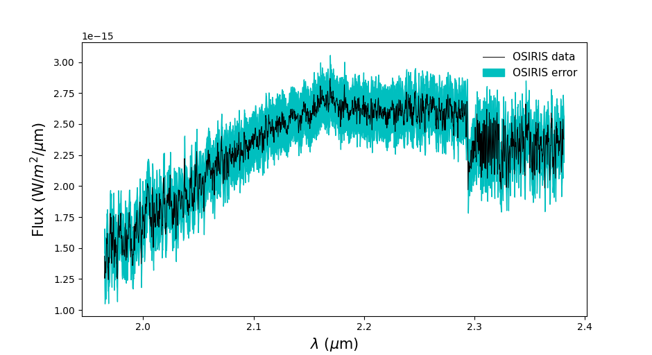
Figure 2: Our fully reduced, combined, and flux calibrated moderate-resolution OSIRIS $K$-band spectra of VHS 1256 b. The errors are derived from the RMS of the individual spectra at each wavelength. Such as error includes uncertainties in both the continuum and the lines, the former of which tends to be larger and is removed via continuum subtraction in portions of our analysis. These total spectral uncertainties are represented as a shaded blue region. The median uncertainty is $\sim$7$\%$ in flux. The CO bandhead is clearly visible at 2.3 $\mu$m.

By removing the continuum, narrow spectral features are more easily analyzed by avoiding low spatial frequency errors that impact the overall continuum shape. We remove the continuum from our fully reduced and flux calibrated spectra using a similar continuum removal strategy we have employed in the past for OSIRIS data (e.g., Barman et al. 2015; Wilcomb et al. 2020). To remove the continuum, we apply a high-pass filter with a kernel size of 200 spectral bins to each of the individual spectra. Then we subtract the smoothed spectrum from the original spectra. Once all the individual spectra are continuum subtracted, we median combine them and find the uncertainties by calculating the RMS of the individual spectra at each wavelength. The median uncertainty on our flattened spectrum is 0.4$\%$, much smaller than the uncertainty on the spectrum with the continuum included.

3 Spectral Modeling

3.1 Synthetic Spectra

In order to determine the atmospheric properties of VHS 1256b, we use models computed through the $PHOENIX$ model atmosphere code (Hauschildt et al., 1999). The atmospheric properties for young gas giants and brown dwarfs are notoriously complex, with cloud modeling being particularly challenging. In our modeling framework, we are able to parameterize clouds in several different ways. They are incorporated as a thick cloud layer with a log-normal ISM-like grain size distribution in all three types of cloud models; DUSTY (Allard et al., 2001), COND (Allard et al., 2001), and an Intermediate Cloud Model (ICM) (Barman et al., 2011). DUSTY models have inefficient gravitational settling so dust is still in the atmosphere, and COND models have efficient gravitational settling therefore no dust is left in the atmosphere. For VHS 1256 b, we used an ICM approach that has a base pressure set by equilibrium chemistry. The vertical extent of the cloud is parameterized by a pressure value that, when above the value, allows the cloud particles number density to fall off exponentially. The cloud particle sizes follow a log normal distribution that is characterized by a median grain size. We will therefore refer to the custom grid constructed here as PHOENIX-ICM to distinguish it from other models based on the PHOENIX framework. We also used two other grids to fit the data; PHOENIX-ACES, the custom grid used for $\kappa$ And b (Wilcomb et al., 2020), and PHOENIX-HR8799, the custom grid used in Ruffio et al. (2021). We explore the results of our choice of cloud model and describe the fits from a few other models in Section 4.

Our first goal is to constrain the temperature, surface gravity, and cloud parameters of VHS 1256 b. In order to do this, we must construct a model grid that spans the expected values of these parameters. In a number of previous works on VHS 1256 b, the temperature was estimated to be in the range of 800–1200 K and the surface gravity ($\log g$) 3.2–4.5 (e.g., Miles et al., 2018; Gauza et al., 2015).

Based on these measurements, we generated a custom PHOENIX grid. The details on the computation of this grid are described in Barman et al. (2011, 2015), with the updated methane line list from Hargreaves et al. (2020) and the optical opacities from Karkoschka & Tomasko (2010). The grid spans a temperature range 800–2100 K, a $\log g$ range of 3.5–5.5 dex, and a cloud property range $P_{cloud}$ dyne/cm² of 5$\times$10⁵–4$\times$10⁶, which encompasses the values previously reported for VHS 1256 b. Vertical mixing (Kzz) was modeled in Miles et al. (2018) and was determined to be $\sim$ 10⁸ cm²s^-1 because with a cooler object of about 1200 K some of the C will still be in CH₄, and therefore CO will not be constant with height. This custom grid also varied grain size, but initially we used a fixed mean grain size of 0.5 $\mu$m.

The synthetic spectra from the grid were calculated with a wavelength sampling of 0.05 Å from 1.4 to 2.4 $\mu$m. Each spectrum was convolved with a Gaussian kernel with a FWHM that matched the OSIRIS spectral resolution (Barman et al., 2011). Both flux calibrated and continuum subtracted data were modeled and analyzed. The synthetic spectra were flux calibrated and continuum subtracted using the same routines as the data.

3.2 Forward Modeling

To determine the best-fit model for each grid, we use a forward-modeling approach following Blake et al. (2010), Burgasser et al. (2016), Hsu et al. (2021b), and Theissen et al. (2022) The effective temperature ($T_{\mathrm{eff}}$), surface gravity ($\log g$), and cloud parameter ($\log P_{cloud}$) are inferred using a Markov Chain Monte Carlo (MCMC) method built on the emcee package that uses an implementation of the affine-invariant ensemble sampler (Goodman & Weare, 2010; Foreman-Mackey et al., 2013). The assumptions and description of the MCMC calculations are described in Wilcomb et al. (2020).

We also forward modeled the primary, VHS 1256 AB, spectra from Gauza et al. (2015). The data span 0.47–1.35 $\mu$m, 1.48–1.78 $\mu$m, and 1.95–2.41 $\mu$m. Since they are a late-M binary pair, we used the Göttingen spectral library (Husser et al., 2013) that varies the effective temperature ($T_{\mathrm{eff}}$), surface gravity ($\log g$), and metallicity ([M/H]) and covers the range of values expected for an M star. The results show that the host binary has approximately solar metallicity. The best fit parameters for VHS1256AB from $K$-band data are $T_{\mathrm{eff}}$ = 2756${}^{+13}_{-15}$ K, $\log g$ = 4.99${}^{+0.0076}_{-0.013}$, and [M/H] = 0.0093${}^{+0.012}_{-0.0063}$. For the short wavelength data the best fit parameters are $T_{\mathrm{eff}}$ = 2668${}^{+8}_{-7}$ K, $\log g$ = 3.57$\pm 0.060$, and [M/H] = 0.20$\pm 0.040$. The $H$-band data best fit parameters are $T_{\mathrm{eff}}$ = 2758${}^{+15}_{-18}$ K, $\log g$ = 3.92${}^{+0.090}_{-0.40}$, and [M/H] = 0.39${}^{+0.14}_{-0.35}$. Since there is no higher resolution data available for the host binary, our precision in metallicity or abundance measurements is limited and further discussion about the systematics in the uncertainties is in Section 3.3. We report the allowed values of these fits to be an effective temperature of 2661 – 2773 K, a surface gravity of 3.51 – 5.00, and an [M/H] of 0.0030 – 0.53. The full results of the fits are shown in Table 2.

3.3 Temperature, Gravity, and Cloud Parameters

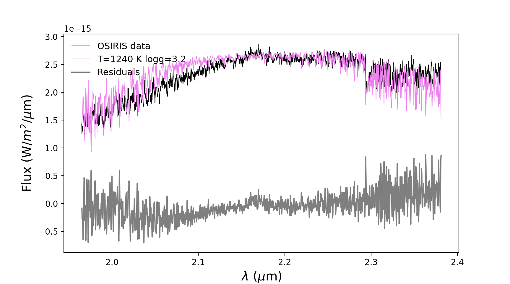
Figure 3: Our fully reduced, combined, and flux calibrated moderate-resolution OSIRIS $K$-band spectra of VHS 1256 b in black plotted alongside our best-fit model in pink. The residuals are shown below in gray. Even our custom PHOENIX-ICM had trouble fitting the continuum of our spectrum, specifically on the bluer end. However, this grid still provided the lowest residuals of any we considered.

We ran our MCMC fitting procedure on both the flux calibrated spectrum and the continuum-subtracted spectrum of VHS 1256b. Objects like VHS 1256b that straddle the L/T transition are notoriously difficult to fit with an unconstrained MCMC, primarily due to the complexity of modeling the clouds at low surface gravities (e.g., Barman et al. 2011). Therefore, we constrained the bounds of the fits via two methods. First, we used previously derived literature values for temperature and surface gravity as a starting point for a plausible range of values (e.g., Gauza et al. 2015; Miles et al. 2018). Then, we plotted the models in those temperature ranges over the data to verify by-eye that the matches were reasonable before running the full MCMC. We therefore narrowed the prior ranges for the temperature to be between 1000-1300 K and a $\log g$ between 3.0-3.5. The best-fit parameters for our flux calibrated data are $T_{\mathrm{eff}}=1240^{+1}_{-2}$ K, $\log g=3.25^{+0.01}_{-0.1}$, and $\log P_{cloud}$ = $6\pm 0.01$. For the radius, which comes from the multiplicative flux parameter, we found R = 1.00 $\pm$ 0.02 R_Jup. For our continuum-subtracted data the best-fit parameters were $T_{\mathrm{eff}}=1223^{+1}_{-2}1$ K, $\log g=3.6^{+0.02}_{-0.01}$, and $\log P_{cloud}$ = $6.6^{+0.07}_{-0.05}$. Radii cannot be derived for the continuum-subtracted data. Figures 3 through 5 show the best-fit spectra overplotted on our data, the residuals from the fits, and the resulting corner plot from our MCMC analysis for the continuum-subtracted spectra.

In order to verify that the temperature estimates we derived from the OSIRIS spectra are robust, we ran our MCMC fitting code using the three custom PHOENIX grids on the Gauza et al. (2015) optical, $J$-band, $H$-band, and $K$-band spectra and the Miles et al. (2018) $L$-band spectra shown in Table 2. We adjusted our MCMC parameters for the Gauza et al. (2015) spectra by setting the line-spread function (LSF) to 229.77 km s^-1, which we derived from the data. We fit each band in the data set separately and obtained $T_{\mathrm{eff}}=1201^{+2}_{-1}$ K, $\log g=4.81\pm 0.06$, and $\log P_{cloud}$ = $6.59\pm 0.01$ for the optical+$J$ band spectra, $T_{\mathrm{eff}}=1281^{12}_{-23}$ K, $\log g=3.67^{+0.05}_{-0.04}$, and $\log P_{cloud}$ = $6.06\pm 0.02$ for the $K$-band spectra, and $T_{\mathrm{eff}}=1201^{+2}_{-1}$ K, $\log g=3.51\pm 0.01$, and $\log P_{cloud}$ = $5.97^{+0.02}_{-0.03}$ for the $H$-band spectra using our custom PHOENIX-ICM grid. We also adjusted our MCMC parameters for the Miles et al. (2018) by using an LSF of 106.95 km s^-1 to account for the lower resolution of the data and obtained an $T_{\mathrm{eff}}=1205^{+7}_{-4}$ K, $\log g=3.53^{+0.03}_{-0.02}$, and $\log P_{cloud}$ = $6.23\pm 0.02$.

Since our subsequent analysis of the chemical abundances of VHS 1256 b relies on knowledge of the temperature and gravity, we did additional modeling to look at the comparison between our custom cloud model grid and similar grids with different treatment of clouds. In addition to differences in cloud parameters, each grid of models incorporates different assumptions that lead to systematic differences in the output spectra for the same parameters such as temperature and gravity (e.g., Oreshenko et al. 2020). These systematics are not captured in the uncertainties that come from each MCMC run output, and therefore those uncertainties, while reported here for completeness, are underestimates of the true uncertainties. These systematics also partially explain why fitting different parts of the spectra give slightly different best fit values, a very common occurrence for substellar object fits (e.g.,Cruz et al. 2018). We attempt to account for these systematics by looking at the range of values given from the three PHOENIX grids.

We incorporated our PHOENIX-ACES grid from Wilcomb et al. (2020) and the PHOENIX-HR8799 grid from Ruffio et al. (2021) into our MCMC analysis code, and fit our OSIRIS spectrum using the same procedure described above. The best-fit using PHOENIX-ACES yielded $T_{\mathrm{eff}}=1500\pm 5$ K and $\log g=3.92^{+0.06}_{-0.08}$. The PHOENIX-HR8799 models generally provided poor matches to the higher resolution data, yielding much higher residuals than other grids. With this grid, we found $T_{\mathrm{eff}}=820^{+2}_{-2}$ K and $\log g=3.01^{+0.02}_{-0.01}$ as best-fit parameters. We found no fits with PHOENIX-HR8799 that properly captured the continuum shape of our OSIRIS data. The fits to the continuum were generally poor across all grids, including the PHOENIX-ICM grid, and we speculated that this was due to our assumption about grain size in the models (see Section 3.3.1). We also fit the three Gauza et al. (2015) spectra and the Miles et al. (2018) spectra with these additional grids. The PHOENIX-HR8799 grid did a poor job of fitting the Miles et al. (2018) spectra, while the PHOENIX-ACES grid fit the data well but gave unphysical parameters when the radii were derived shown in Table 3. Overall, the PHOENIX-ICM grid fit the spectra of this object the best and we adopt the values from these fits in this paper.

Table 3 shows the results for all atmospheric parameters derived in this paper. We use the range of best-fit values from the OSIRIS continuum-included data to define the adopted parameters for temperature, gravity, and cloud parameter, as the resolved line information coupled with the continuum offers the most constraints on those parameters. To derive more robust uncertainties on the atmospheric parameters that account for the systematics described above, we consider the range of values from all fits using the PHOENIX-ICM grid when deriving th allowed values for VHS 1256b. We adopt values of $T_{\mathrm{eff}}=1240$ K, with a range of 1200–1300 K, $\log g=3.25$, with a range of 3.25–3.75, and $\log P_{cloud}$ = $6.0$, with a range of 6.0–6.6. For radius, we use the median value from the OSIRIS continuum-included data and the Gauza et al. (2015) spectra to arrive at $R=1.0~{}R_{Jup}$, with a range of 1.0–1.2 $R_{Jup}$. This yields an implied bolometric luminosity of log(L/L_⊙) = $4.67$, with a range of $4.60$ to $4.70$. These values are all in excellent agreement with previous studies (Gauza et al., 2015; Miles et al., 2018).

3.3.1 Cloud Grain Size

VHS 1256 b is an L/T transition object, and these objects spectra are strongly impacted by the depth of clouds and the grain size in the atmosphere (Brock et al., 2021). Since our custom PHOENIX-ICM grid also varied in grain size, we explored different mean grain sizes to get a better fit to the continuum in our OSIRIS data, as well as a better match to data in all wavebands. We held all other parameters constant, except for the multiplicative factor that is a proxy for radius, and allowed the mean grain size to vary from 0.5 $\mu$m to 3 $\mu$m. For our OSIRIS data, the best fit grain size was about 3${}^{+0}_{0.1}\mu$m, which did hit the edge of our grid. For the Gauza et al. (2015) spectra, the best fit grain size was 0.51${}^{+0.02}_{-0.0094}\mu$m at the short wavelengths, 0.50${}^{+0.010}_{-0.0048}\mu$m for the $H$-band spectrum, and 0.99${}^{+0.018}_{-0.032}$ for the $K$-band spectrum. The best fit grain size for the Miles et al. (2018) spectrum was 0.51${}^{+0.11}_{-0.01}\mu$m.

Since the fits to the short and long wavelength data yielded different preferred grain sizes than the OSIRIS data, we examined both 0.5 $\mu$m and 3.0 $\mu$m models across the full range of available wavelengths simultaneously. Figure 2 shows all available spectral and photometric data for VHS 1256 b. Overplotted are the two PHOENIX-ICM models with two different grain sizes, 0.5 $\mu$m and 3 $\mu$m. The models are scaled to match the continuum flux at $K$-band, which in turn is derived using the $K$-band magnitude in Gauza et al. ($K_{s}=14.665\pm 0.01$; 2015). First, we note that the lower resolution $K$ band spectra from Gauza et al. (2015) spectra are a good overall match to the OSIRIS data. We note that when we look at the model in comparison to the flux calibrated shorter wavelength data, the 3 $\mu$m grain size model is a good match overall though not a perfect match to the continuum shape. However, the 0.5 $\mu$m model, the model strongly underpredicts the short wavelength flux if it is scaled to match $K$ band. This means that the best-fit of 0.5 $\mu$m at these short wavelengths was dependent on scaling the radius to much larger values was required for the $K$ band. Indeed, with a the best-fit value for $K$ band is a radius of $\sim$1 R_Jup, whereas the best fit at short wavelengths with a small grain size is $\sim$1.4 R_Jup. This implies that the fits were being pulled by the continuum shape when performed individually, and a comprehensive look at data at all wavelengths is more appropriate for determining the grain size. We do note that in the case of the long wavelength data from Miles et al. (2018) spectra and the photometry from Rich et al. (2016), the red side of the spectrum matches the 0.5 $\mu$m model better, and the radius is consistent with $K$ band and roughly the same for either grain size. However, the overall shape of the Miles et al. (2018) spectrum does not match either model. Taken together, we conclude that a larger median grain size of 3.0 $\mu$m is appropriate for this object.

3.4 Mole Fractions of CO, H₂O, and CH₄

With best fit values for temperature, surface gravity, and clouds, we can derive abundances of CO, H₂O, and CH₄ using our OSIRIS $K$-band spectra. Once best fit values were determined for $T_{\mathrm{eff}}$, $\log g$, and $\log P_{cloud}$, we fixed those parameters to generate a grid of spectra with scaled mole fractions of these molecules, which are visible in the $K$-band (Barman et al., 2015). We used solar metallicity for this grid because there is no evidence for non-solar metallicity. Therefore, the unscaled mixing ratios in this grid will match the composition and mole fractions of the Sun. The molecular abundances of CO, CH₄, and H₂O were scaled relative to their initial values from 0 to 1000 using a uniform logarithmic sampling, resulting in 25 synthetic spectra. We fit for the mole fraction of H₂O first, holding CO and CH₄ at their initial values. Next, the H₂O mole fraction was set to its nominal value, and we fit for scaled CO. We did the same analysis for CH₄.

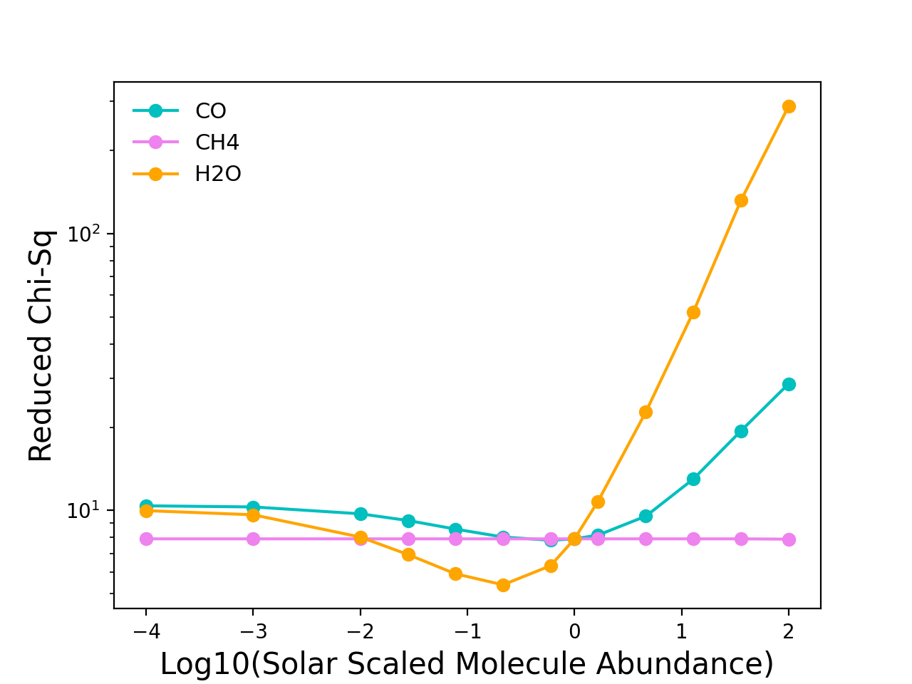
Figure 7: Results of $T_{\mathrm{eff}}$ = 1240 K, $\log g$ = 3.25, $\log P_{cloud}$ = 6, and grain size = 3 $\mu$m model fits with varying mole fractions for both H₂O, CO, and CH₄ to our continuum-subtracted OSIRIS spectrum. The mole fractions are given in units relative to the ratio in the Sun, such that a value of zero implies the solar value. The scalings of CO prefer solar/subsolar and the scalings of H₂O prefer values subsolar. From these fits we find C/O = 0.869${}_{-0.24}^{+0.09}$.

Figure 7 shows the resulting $\chi^{2}$ distribution as a function of CO, H₂O, and CH₄ mole fraction. The models with the lowest $\chi^{2}$ when compared to the flattened data gave us the best-fits for both H₂O and CO. For CH₄, there is no change in $\chi^{2}$ with any change in the mole fraction, suggesting that if any methane is present in the spectrum, it is below the detection threshold of our data. We exclude CH₄ from further analysis. The best fit for H₂O had a scaling of 0.215${}^{+0.784}_{-0.187}$, and the best fit for CO had a scaling of 0.599${}^{+1.061}_{-0.384}$. To calculate the 1-$\sigma$ uncertainties in each mole fraction value, we used the values from models within $\pm$1 of our lowest $\chi^{2}$.

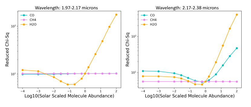
Figure 8: Left: The results of our $\chi^{2}$ analysis on the first half of our continuum subtracted OSIRIS data. The CO abundances vary minimally during this analysis because of the lack of CO lines in the first half of our spectra. The best-fit water is still subsolar, with the lowest $\chi^{2}$ values not including solar. Right: The results of our $\chi^{2}$ analysis on the second half of our continuum subtracted OSIRIS data. The values allowed by the $\chi^{2}$ analysis include the solar abundance model, with the best-fit H₂O molecular abundance being slightly subsolar.

Because of the potential issues with telluric correction in the blue side of the spectrum mentioned in Section 2, we explored the mole fractions on different portions of the spectra, splitting it in half and performing the fit again. Shown in the left panel of Figure 8, for the first half of the spectrum, the best fit H₂O mole fraction is 0.215 and CO is unchanging as there are no CO features in this section of the spectra. For the second half of the OSIRIS spectra, shown in right panel of Figure 8, the H₂O scaled mole fraction is higher at 0.599 and the uncertainties encompass the lowest $\chi^{2}$ from the full spectrum analysis. The lowest $\chi^{2}$ CO matches the values found when fitting the full spectrum (Figure 7). Because of concerns about the blue half of the spectrum, we elect to use the C and O values from the second half of the spectrum. This yields an H₂O mole fraction of 0.599${}^{+0.401}_{-0.384}$ and a CO mole fraction of 0.599${}^{+1.061}_{-0.384}$.

3.5 C/O Ratios

In our previous work, we have used OSIRIS data to constrain the C/O ratios of directly imaged companions to massive stars such as HR 8799 b, c, and d, and $\kappa$ Andromedae b (e.g., Konopacky et al. 2013; Wilcomb et al. 2020; Ruffio et al. 2021). For giant planets formed by rapid gravitational instabilities, their atmospheres should have elemental abundances that are the same as their host stars (Helled & Schubert, 2009). If giant planets form by a multi-step core accretion process, it has been suggested that there could be a range of elemental abundances possible (Öberg et al., 2011; Madhusudhan, 2019). In this scenario, the abundances of giant planets’ atmospheres formed by core/pebble accretion are highly dependent on the location of formation relative to CO, CO₂, and H₂O frost lines and the amount of solids acquired by the planet during runaway accretion phase. This can be diagnosed using the C/O ratio.

For VHS 1256 b, a substellar companion to a small binary pair, it is unclear if C/O is a useful formation diagnostic, as it is likely to have formed like a binary star rather than a planet (see Section 4). However, we still compute the ratio here and discuss the implications below.

The C/O ratio dependence on atmospheric mole fractions (N) is

$$\frac{C}{O}=\frac{N(CH_{4})+N(CO)}{N(H_{2}O)+N(CO)},$$

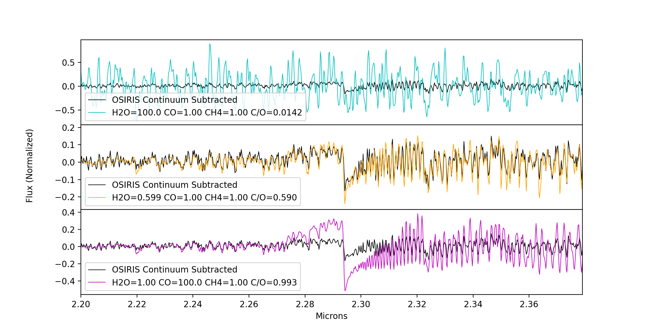
Figure 9: Our fully reduced, combined, and continuum subtracted moderate-resolution OSIRIS $K$-band spectra of VHS 1256 b plotted alongside three models of T=1240 K and $\log g$=3.2 with varying C/O. The top panel shows the super-solar H₂O model with C/O=0.0142 in blue. The middle panel shows our best fit model with subsolar H₂O and solar CO and CH₄, which gives C/O=0.590. The bottom panel shows a supersolar CO model with C/O=0.993. This demonstrates how well moderate resolution spectroscopy can constrain C/O ratios of planetary mass objects.

and for small amounts of CH₄, as in VHS 1256 b’s case, the C/O ratio can be determined by H₂O and CO alone (Barman et al., 2015). The C/O ratio we derive for VHS 1256 b is 0.590${}_{-0.384}^{+0.280}$. The large uncertainties encompass potential systematics and any differences in C/O ratio from the two halves of the spectrum. Variability of the object is unlikely to affect the measurement of C/O because CO is formed higher in the atmosphere than the predicted location of cloud decks. The variability at K band has been shown to be less significant than at other wavelengths (e.g., Vos et al. 2019; Bowler et al. 2020). Figure 9 shows our lowest $\chi^{2}$ model in the center panel and two extreme cases to illustrate the sensitivity our OSIRIS moderate resolution spectra has to the C/O ratio.

4 Discussion and Conclusions

Moderate resolution spectroscopy has expanded our knowledge of young directly imaged planet atmospheres. VHS 1256 b provides an interesting diagnostic because of the low contrast between the companion and the host system, and the thick cloudy atmosphere. Our results of $T_{\mathrm{eff}}=1240$ K, with a range of 1200–1300 K, and $\log g=3.25$, with a range of 3.25–3.75 agree with the results from Gauza et al. (2015) that posit VHS 1256 b is a low surface gravity object and is likely a planetary mass object in a youthful system. Our effective temperature is also in agreement with the literature regardless of the new distance measured by Gaia EDR3, 22.2${}^{+1.1}_{-1.2}$ pc, which changed the distance from 12.7$\pm$1.0 pc (Gauza et al., 2015). Dupuy et al. (2020) also found a distance 22.22 $\pm$ 1.19 pc from CFHT parallax measurements. We did not detect methane in our $K$-band spectra, which is in agreement with very weak methane absorption in the $L$-band spectra pointing towards non-equilibrium chemistry from Miles et al. (2018).

Our OSIRIS data on VHS 1256 b, coupled with data from the literature, preferred a thick-cloud model, $\log P_{cloud}$ = $6.0$ with a range of 6.0–6.6, with a 3 $\mu$m mean grain size. Recent works have demonstrated that earlier L-type objects have higher-altitude clouds with smaller grains (0.25–0.50 $\mu$m), and later T-type objects exhibit deeper clouds and larger grains ($\geq$ 1 $\mu$m; Brock et al. 2021). We conclude that VHS 1256 b has deep clouds with a large mean grain size that is consistent with being near or just beyond the L/T transition, as indicated by its L7 spectral type.

Cloudy atmospheres of these Jovian-like objects are not well understood. Data at longer wavelengths can more deeply probe these cloud parameters and can inform the models to better understand the processes occurring in cloudy giant planet atmospheres. VHS 1256 b is also extremely variable with near infrared photometry in 2MASS J, H, and K/K_s that varies by $\sim$37, $\sim$13, and $\sim$3 percent respectively (Miles et al., 2018). This can lead to different colors and flux calibrations that can influence interpreted atmospheric parameters. Understanding the variability of this object is important for further constraints on effective temperature and other atmospheric parameters. Our derivation of cloud properties, including a notional grain size distribution, will inform studies of variability of VHS 1256 b.

Formation of objects in the gas giant planet mass regime is of considerable interest, whether the companion orbits a low or high mass star. Formation diagnostics such as C/O ratio can provide context and potentially point to a formation pathway, although interpretation of the C/O ratio is complicated by a variety of phenomena (e.g., Madhusudhan 2019). The mass ratio of the system is 0.16, which is significantly larger than other directly imaged planets such as HR 8799 (q $\sim$ 5 $\times$ $10^{-3}$; Fabrycky & Murray-Clay 2010) suggesting that the companion was likely too large to form in a protoplanetary disk around the primary (Rich et al., 2016). In measuring the C/O ratio here for VHS 1256 b, we seek instead to use observations of a similar object to the directly imaged planets to look for systematics in our modeling that could suggest any biases in computation of C/O. We derived a C/O ratio of 0.590${}_{-0.384}^{+0.280}$ for VHS 1256 b. Our finding of a roughly solar C/O ratio implies that these systematics are not present, which would be suggested by a ratio that is very different from solar. An unusual C/O ratio compared to the stellar value in a low mass binary is unexpected, and would suggest issues with modeling L/T transition objects. It is likely that VHS 1256 b formed like a binary star rather than a planet. There are studies that claim metallicity measurements could constrain formation location for these types of objects, but future work is needed to obtain these measurements for the host binary and the wide orbit companion (Liu et al., 2021). While we do not measure a C/O ratio for the host star because we did not have moderate resolution spectroscopy for it, there is no indication that a non-solar metallicity is required to describe the spectra in hand (Gauza et al., 2015). Thus, we are confident our methodology is sound and reliably provides C/O ratios for directly imaged companions. Indeed, Figure 9 shows that very large or small C/O ratios are easily probed and ruled out by moderate-to-high resolution data, and are thus more trustworthy than values computed on low resolution spectra.

VHS 1256 b now represents an eighth case of an imaged planetary mass object, in addition to the four HR 8799 planets (Konopacky et al., 2013; Barman et al., 2015; Mollière et al., 2020; Ruffio et al., 2021), $\kappa$ And b (Wilcomb et al., 2020), HIP 65426 b (Petrus et al., 2021), and TYC 8998-760-1 b (YSES-1 b Zhang et al. 2021), where the C/O ratio formation diagnostic did not reveal ratios that clearly point to formation via core/pebble accretion. The scenario cannot be completely ruled out given the uncertainties in the data and the range of possible C/O ratios predicted by models (e.g., Madhusudhan 2019). Therefore, other probes of formation such as the ¹²CO/¹³CO isotope ratio (Zhang et al., 2021) and metallicity, will be needed to shed more light on this intriguing population of giant companions.

VHS 1256 b has already been targeted with a higher resolution instrument, NIRSPEC at the Keck II 10 m telescope, which allowed for measurements of radial velocity and rotational velocity (Bryan et al., 2018). The next steps for the VHS 1256 system will be space-based spectroscopy to verify the C/O ratio and other atmospheric properties. VHS 1256 b is a target for the High Contrast Imaging of Exoplanets and Exoplanetary Systems with JWST Early Release Science (ERS) Program (Hinkley et al., 2017). VHS 1256 b will be studied using NIRSpec and MIRI to analyze the atmosphere at longer wavelengths to constrain non-equilibirum chemistry, C/O ratio, and variability of the object. We can also determine whether the bulk population of directly imaged planets show C/O ratios consistent with solar/stellar values by continuing to obtain moderate- or high-resolution spectra of these wide orbit, self-luminous companions. If the population of these objects show distinct C/O from closer in transit giant planets, this could point towards differing formation pathways for these companions.

Table 1: Summary of VHS 1256 AB b System

Parameter	Central Binary	Companion	Reference
Distance (pc)	22.2${}^{+1.1}_{-1.2}$	-
Separation (arcsec)	$0.109\pm 0.0018$	$8.06\pm 0.03$
Projected Separation (au)	$2.42\pm 0.0399$	$102\pm 9$
Spectral Type	M7.5$\pm 0.5$	L7.0$\pm 1.5$
Apparent Magnitudes
2MASS $J$-band	11.018$\pm 0.023$	16.662$\pm 0.287$
2MASS $H$-band	10.473$\pm 0.023$	15.595$\pm 0.209$
2MASS $K_{s}$-band	10.044$\pm 0.021$	14.568$\pm 0.121$
VHS $Y$-band	$<11.72$	18.558$\pm 0.051$
VHS $J$-band	$<11.36$	17.136$\pm 0.020$
VHS $H$-band	$<11.02$	15.777$\pm 0.015$
VHS $K_{s}$-band	$<10.42$	14.665$\pm 0.010$
Subaru/IRCS $L$-band	9.76$\pm 0.03$	12.99$\pm 0.04$

References. — (a) Dupuy et al. (2020), (b) Stone et al. (2016), (c) Gauza et al. (2015), (d) Skrutskie et al. (2006), (e) McMahon et al. (2013), (f) Rich et al. (2016)

Table 2: Summary of atmospheric parameters derived from MCMC fits for the Primary.

Spectra	Effective Temperature	Surface Gravity	Metallicity
VHS 1256 b	${T}_{\mathrm{{eff}}}$ (K)	$\log g$	$M/H$
Göttingen PHOENIX Spectral Library
Gauza Primary $K$-band	$2756^{+13}_{-15}$	$4.99^{+0.0076}_{-0.015}$	$0.0093^{+0.012}_{-0.0063}$
Gauza Primary Optical+$J$ band	$2668^{+8}_{-7}$	$3.57\pm 0.060$	$0.20\pm 0.040$
Gauza Primary $H$-band	$2758^{+15}_{-18}$	$3.92^{+0.090}_{-0.40}$	$0.39^{+0.14}_{-0.35}$
Allowed Range of Values	2661 - 2773	3.51 - 5.00	0.0030 - 0.53

Table 3: Summary of atmospheric parameters derived from MCMC fits.

Spectra	Effective Temperature	Surface Gravity	Cloud Layer	Grain size	Radius	Luminosity
VHS 1256 b	${T}_{\mathrm{{eff}}}$ (K)	$\log g$	$\log P_{cloud}$	$\mu$m	($R_{\mathrm{Jup}}$)	$\log_{10}\left(\frac{L}{L_{\odot}}\right)$
PHOENIX-ACES
OSIRIS Including Continuum	$1500^{+5}_{-5}$	$3.92^{+0.06}_{-0.08}$	n/a	n/a	$0.64$	$-4.73$
OSIRIS Continuum Subtracted	$1500^{+5}_{-5}$	$4.47^{+0.01}_{-0.02}$	n/a	n/a	n/a	n/a
Gauza $K$-band	$1839^{+6}_{-7}$	$4.83^{+0.01}_{-0.02}$	n/a	n/a	$0.41$	$-4.76$
Gauza Optical+$J$ band	$1659^{+3}_{-3}$	$3.72^{+0.01}_{-0.01}$	n/a	n/a	$0.52$	$-4.73$
Gauza $H$-band	$1658^{+2}_{-2}$	$4.65^{+0.02}_{-0.02}$	n/a	n/a	$0.54$	$-4.70$
Miles $L$-band	$1096^{+12}_{-13}$	$4.38^{+0.11}_{-0.13}$	n/a	n/a	$1.18$	$-4.74$
PHOENIX-ICM
OSIRIS Including Continuum	$1240^{+1}_{-2}$	$3.25^{+0.01}_{-0.1}$	$6.0\pm 0.01$	$3.0\pm 0.1$	$1.0$	$-4.67$
OSIRIS Continuum Subtracted	$1223^{+1}_{-2}$	$3.6^{+0.02}_{-0.01}$	$6.6^{+0.07}_{-0.05}$	$2.9^{+0.001}_{-0.01}$	n/a	n/a
Gauza $K$-band	$1281^{+12}_{-23}$	$3.67^{+0.05}_{-0.04}$	$6.06\pm 0.02$	$0.99^{+0.018}_{-0.032}$	$0.92$	$-4.69$
Gauza Optical+$J$-band	$1201^{+2}_{-1}$	$4.81^{+0.06}_{-0.06}$	$6.59\pm 0.01$	$0.51^{0.02}_{0.0094}$	$1.2$	$-4.57$
Gauza $H$-band	$1201^{+2}_{-1}$	$3.51^{+0.01}_{-0.01}$	$5.97^{+0.02}_{-0.03}$	$0.05^{+0.010}_{-0.0048}$	$1.18$	$-4.58$
Miles $L$-band	$1205^{+7}_{-4}$	$3.53^{+0.03}_{-0.02}$	$6.23\pm 0.02$	$0.51^{+0.11}_{-0.01}$	$1.13$	$-4.61$
PHOENIX-HR8799
OSIRIS Including Continuum	$820^{+2}_{-2}$	$3.01^{+0.02}_{-0.01}$	$5.7^{+0}_{-0}$	n/a	$2.9$	$-4.46$
OSIRIS Continuum Subtracted	$1300^{+1}_{-2}$	$3.0^{+0.02}_{-0.0}$	$6.0^{+0.01}_{-0.01}$	n/a	n/a	n/a
Gauza $K$-band	$1298^{+1}_{-3}$	$3.28^{+0.02}_{-0.02}$	$5.7^{+0.01}_{-0.0}$	n/a	$0.9$	$-4.68$
Gauza Optical+$J$-band	$1097^{+17}_{-21}$	$3.28^{+0.28}_{-0.16}$	$5.96^{+0.14}_{-0.13}$	n/a	$1.8$	$-4.37$
Gauza $H$-band	$1031^{+9}_{-10}$	$3.01^{+0.02}_{-0.01}$	$5.84^{+0.04}_{-0.03}$	n/a	$1.8$	$-4.48$
Miles $L$-band	$836^{+7}_{-5}$	$3.06^{+0.01}_{-0.01}$	$5.71^{+0.02}_{-0.01}$	n/a	$2.1$	$-4.71$
Adopted Values	1240	3.25	6.0	3.0	1.0	-4.67
Allowed Range of Values	1200 - 1300	3.25 - 3.75	6.0 - 6.6	1.0 - 3.0	1.0 - 1.2	-4.60 - -4.70

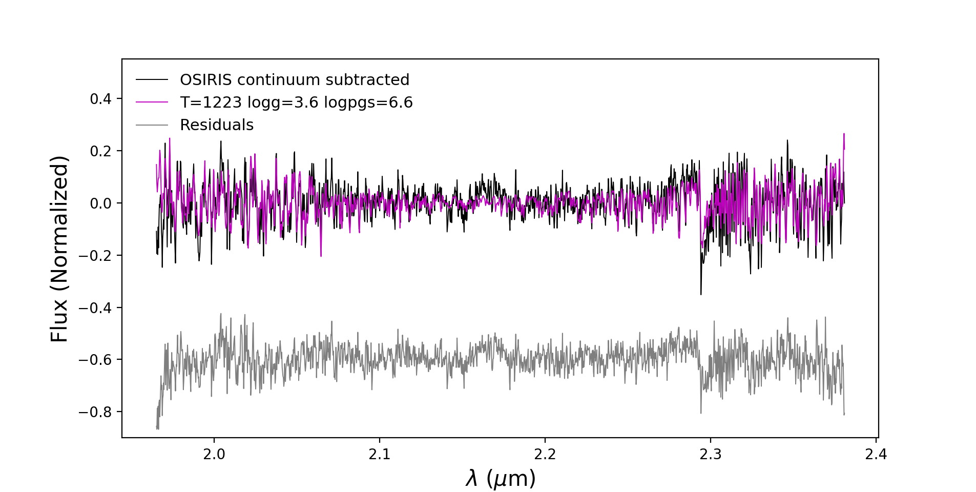
Figure 4: Our OSIRIS continuum subtracted $K$-band spectra in black plotted against our MCMC best-fit model in magenta. The bump in the center of the spectrum between 2.1 and 2.2 $\mu$m is due to residual telluric. By removing the continuum, we remove uncertainties that were tied to the continuum, thus the residuals for the flatted fit are much smaller.

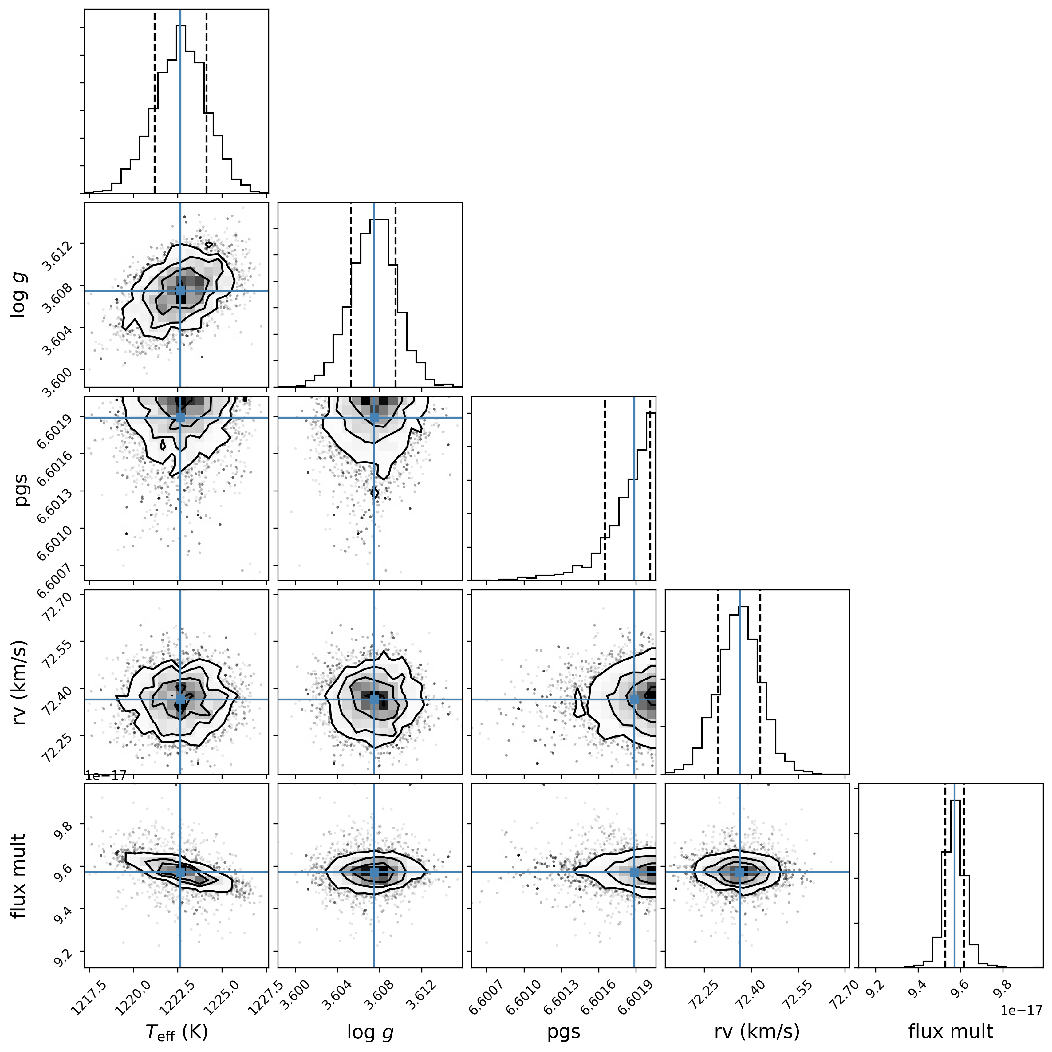
Figure 5: Corner plot from our MCMC fits for our continuum subtracted OSIRIS $K$-band spectra. The diagonal shows the marginalized posteriors. The covariances between all the parameters are in the corresponding 2-d histograms. The blue lines represent the 50 percentile, and the dotted lines represent the 16 and 84 percentiles. The ”flux mult” corresponds to the dilution factor that scales the model by $(radius)^{2}(distance)^{-2}$. Our fit prefers a value near the edge of the grid for pgs, or, $P_{cloud}$.

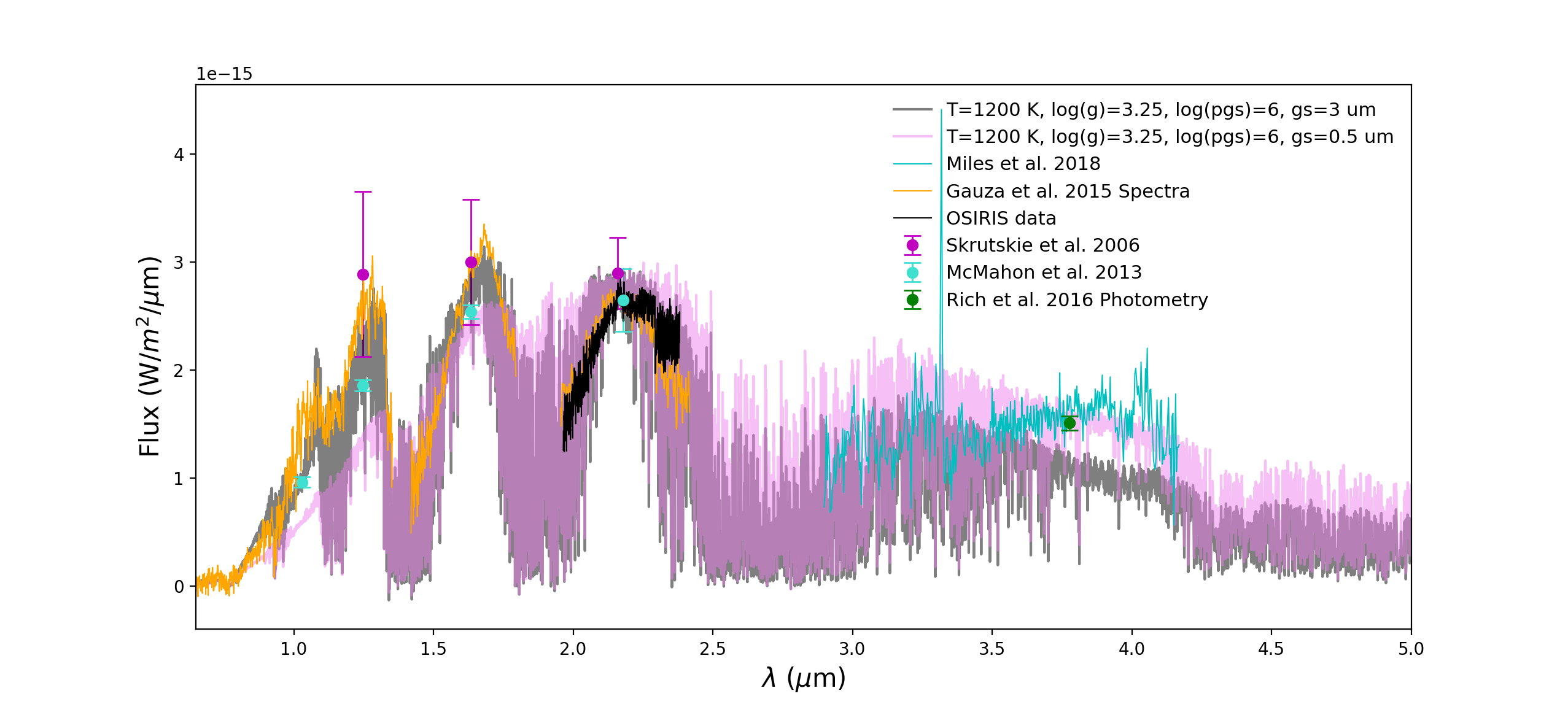
Figure 6: Our fully reduced, combined, and flux calibrated moderate-resolution OSIRIS $K$-band spectra of VHS 1256 b in black, plotted alongside our best fit model with two different grain sizes, 3$\mu$m in gray and 0.5$\mu$m in pink, and spectra from Miles et al. (2018) in blue, spectra from Gauza et al. (2015), and magnitudes from Rich et al. (2016), Skrutskie et al. (2006), and McMahon et al. (2013). The 3 $\mu$m grain size model fits the majority of the data except for the red end of the $L$-band spectra and the Rich et al. (2016) photometry point. The 0.5 $\mu$m grain size model underpredicts the flux in the optical, $J$-, and $H$-band, but does fit the $L$-band spectra and photometry point. We adopt the 3 $\mu$m model as the best-fit for the majority of the available data.

References

- Allard et al. (2001) Allard, F., Hauschildt, P. H., Alexander, D. R., Tamanai, A., & Schweitzer, A. 2001, ApJ, 556, 357, doi: 10.1086/321547
- Bailey et al. (2013) Bailey, V., Hinz, P. M., Currie, T., et al. 2013, ApJ, 767, 31, doi: 10.1088/0004-637X/767/1/31
- Barman et al. (2015) Barman, T. S., Konopacky, Q. M., Macintosh, B., & Marois, C. 2015, ApJ, 804, 61, doi: 10.1088/0004-637X/804/1/61
- Barman et al. (2011) Barman, T. S., Macintosh, B., Konopacky, Q. M., & Marois, C. 2011, ApJ, 733, 65, doi: 10.1088/0004-637X/733/1/65
- Biller et al. (2013) Biller, B. A., Liu, M. C., Wahhaj, Z., et al. 2013, ApJ, 777, 160, doi: 10.1088/0004-637X/777/2/160
- Blake et al. (2010) Blake, C. H., Charbonneau, D., & White, R. J. 2010, ApJ, 723, 684, doi: 10.1088/0004-637X/723/1/684
- Bowler (2016) Bowler, B. P. 2016, PASP, 128, 102001, doi: 10.1088/1538-3873/128/968/102001
- Bowler et al. (2020) Bowler, B. P., Zhou, Y., Morley, C. V., et al. 2020, ApJ, 893, L30, doi: 10.3847/2041-8213/ab8197
- Brock et al. (2021) Brock, L., Barman, T., Konopacky, Q. M., & Stone, J. M. 2021, ApJ, 914, 124, doi: 10.3847/1538-4357/abfc46
- Bryan et al. (2018) Bryan, M. L., Benneke, B., Knutson, H. A., Batygin, K., & Bowler, B. P. 2018, Nature Astronomy, 2, 138, doi: 10.1038/s41550-017-0325-8
- Burgasser et al. (2016) Burgasser, A. J., Lopez, M. A., Mamajek, E. E., et al. 2016, ApJ, 820, 32, doi: 10.3847/0004-637X/820/1/32
- Chin et al. (2012) Chin, J. C. Y., Wizinowich, P., Campbell, R., et al. 2012, in Society of Photo-Optical Instrumentation Engineers (SPIE) Conference Series, Vol. 8447, Adaptive Optics Systems III, ed. B. L. Ellerbroek, E. Marchetti, & J.-P. Véran, 84474F, doi: 10.1117/12.925807
- Cruz et al. (2018) Cruz, K. L., Núñez, A., Burgasser, A. J., et al. 2018, AJ, 155, 34, doi: 10.3847/1538-3881/aa9d8a
- Dupuy et al. (2020) Dupuy, T. J., Liu, M. C., Magnier, E. A., et al. 2020, Research Notes of the American Astronomical Society, 4, 54, doi: 10.3847/2515-5172/ab8942
- Fabrycky & Murray-Clay (2010) Fabrycky, D. C., & Murray-Clay, R. A. 2010, ApJ, 710, 1408, doi: 10.1088/0004-637X/710/2/1408
- Faherty et al. (2013) Faherty, J. K., Rice, E. L., Cruz, K. L., Mamajek, E. E., & Núñez, A. 2013, AJ, 145, 2, doi: 10.1088/0004-6256/145/1/2
- Foreman-Mackey et al. (2013) Foreman-Mackey, D., Conley, A., Meierjurgen Farr, W., et al. 2013, emcee: The MCMC Hammer. http://ascl.net/1303.002
- Galicher et al. (2016) Galicher, R., Marois, C., Macintosh, B., et al. 2016, A&A, 594, A63, doi: 10.1051/0004-6361/201527828
- Gauza et al. (2015) Gauza, B., Béjar, V. J. S., Pérez-Garrido, A., et al. 2015, ApJ, 804, 96, doi: 10.1088/0004-637X/804/2/96
- Goodman & Weare (2010) Goodman, J., & Weare, J. 2010, Communications in Applied Mathematics and Computational Science, 5, 65, doi: 10.2140/camcos.2010.5.65
- Hargreaves et al. (2020) Hargreaves, R. J., Gordon, I. E., Rey, M., et al. 2020, ApJS, 247, 55, doi: 10.3847/1538-4365/ab7a1a
- Hauschildt et al. (1999) Hauschildt, P. H., Allard, F., & Baron, E. 1999, ApJ, 512, 377, doi: 10.1086/306745
- Helled & Schubert (2009) Helled, R., & Schubert, G. 2009, ApJ, 697, 1256, doi: 10.1088/0004-637X/697/2/1256
- Hinkley et al. (2017) Hinkley, S., Baraffe, I., Biller, B., et al. 2017, High Contrast Imaging of Exoplanets and Exoplanetary Systems with JWST, JWST Proposal ID 1386. Cycle 0 Early Release Science
- Hsu et al. (2021a) Hsu, C.-C., Theissen, C., Burgasser, A., & Birky, J. 2021a, SMART: The Spectral Modeling Analysis and RV Tool, v1.0.0, Zenodo, Zenodo, doi: 10.5281/zenodo.4765258
- Hsu et al. (2021b) Hsu, C.-C., Burgasser, A. J., Theissen, C. A., et al. 2021b, ApJS, 257, 45, doi: 10.3847/1538-4365/ac1c7d
- Husser et al. (2013) Husser, T. O., Wende-von Berg, S., Dreizler, S., et al. 2013, A&A, 553, A6, doi: 10.1051/0004-6361/201219058
- Karkoschka & Tomasko (2010) Karkoschka, E., & Tomasko, M. G. 2010, Icarus, 205, 674, doi: 10.1016/j.icarus.2009.07.044
- Konopacky et al. (2013) Konopacky, Q. M., Barman, T. S., Macintosh, B. A., & Marois, C. 2013, Science, 339, 1398, doi: 10.1126/science.1232003
- Krabbe et al. (2004) Krabbe, A., Gasaway, T., Song, I., et al. 2004, in Society of Photo-Optical Instrumentation Engineers (SPIE) Conference Series, Vol. 5492, Ground-based Instrumentation for Astronomy, ed. A. F. M. Moorwood & M. Iye, 1403–1410, doi: 10.1117/12.552592
- Larkin et al. (2006) Larkin, J., Barczys, M., Krabbe, A., et al. 2006, in Society of Photo-Optical Instrumentation Engineers (SPIE) Conference Series, Vol. 6269, Society of Photo-Optical Instrumentation Engineers (SPIE) Conference Series, ed. I. S. McLean & M. Iye, 62691A, doi: 10.1117/12.672061
- Liu et al. (2021) Liu, F., Bitsch, B., Asplund, M., et al. 2021, MNRAS, 508, 1227, doi: 10.1093/mnras/stab2471
- Liu et al. (2016) Liu, M. C., Dupuy, T. J., & Allers, K. N. 2016, ApJ, 833, 96, doi: 10.3847/1538-4357/833/1/96
- Lockhart et al. (2019) Lockhart, K. E., Do, T., Larkin, J. E., et al. 2019, AJ, 157, 75, doi: 10.3847/1538-3881/aaf64e
- Madhusudhan (2019) Madhusudhan, N. 2019, ARA&A, 57, 617, doi: 10.1146/annurev-astro-081817-051846
- McMahon et al. (2013) McMahon, R. G., Banerji, M., Gonzalez, E., et al. 2013, The Messenger, 154, 35
- Miles et al. (2018) Miles, B. E., Skemer, A. J., Barman, T. S., Allers, K. N., & Stone, J. M. 2018, ApJ, 869, 18, doi: 10.3847/1538-4357/aae6cd
- Mollière et al. (2020) Mollière, P., Stolker, T., Lacour, S., et al. 2020, A&A, 640, A131, doi: 10.1051/0004-6361/202038325
- Nielsen et al. (2019) Nielsen, E. L., De Rosa, R. J., Macintosh, B., et al. 2019, AJ, 158, 13, doi: 10.3847/1538-3881/ab16e9
- Nikolov et al. (2018) Nikolov, N., Sing, D. K., Goyal, J., et al. 2018, MNRAS, 474, 1705, doi: 10.1093/mnras/stx2865
- Öberg et al. (2011) Öberg, K. I., Murray-Clay, R., & Bergin, E. A. 2011, ApJ, 743, L16, doi: 10.1088/2041-8205/743/1/L16
- Oreshenko et al. (2020) Oreshenko, M., Kitzmann, D., Márquez-Neila, P., et al. 2020, AJ, 159, 6, doi: 10.3847/1538-3881/ab5955
- Petrus et al. (2021) Petrus, S., Bonnefoy, M., Chauvin, G., et al. 2021, A&A, 648, A59, doi: 10.1051/0004-6361/202038914
- Rameau et al. (2013) Rameau, J., Chauvin, G., Lagrange, A. M., et al. 2013, ApJ, 779, L26, doi: 10.1088/2041-8205/779/2/L26
- Rich et al. (2016) Rich, E. A., Currie, T., Wisniewski, J. P., et al. 2016, ApJ, 830, 114, doi: 10.3847/0004-637X/830/2/114
- Ruffio et al. (2021) Ruffio, J.-B., Konopacky, Q. M., Barman, T., et al. 2021, arXiv e-prints, arXiv:2109.07614. https://arxiv.org/abs/2109.07614
- Skrutskie et al. (2006) Skrutskie, M. F., Cutri, R. M., Stiening, R., et al. 2006, AJ, 131, 1163, doi: 10.1086/498708
- Stone et al. (2016) Stone, J. M., Skemer, A. J., Kratter, K. M., et al. 2016, ApJ, 818, L12, doi: 10.3847/2041-8205/818/1/L12
- Theissen et al. (2022) Theissen, C. A., Konopacky, Q. M., Lu, J. R., et al. 2022, ApJ, 926, 141, doi: 10.3847/1538-4357/ac3252
- Vigan et al. (2021) Vigan, A., Fontanive, C., Meyer, M., et al. 2021, A&A, 651, A72, doi: 10.1051/0004-6361/202038107
- Vos et al. (2019) Vos, J. M., Biller, B. A., Bonavita, M., et al. 2019, MNRAS, 483, 480, doi: 10.1093/mnras/sty3123
- Wang et al. (2022) Wang, J., Kolecki, J. R., Ruffio, J.-B., et al. 2022, AJ, 163, 189, doi: 10.3847/1538-3881/ac56e2
- Wilcomb et al. (2020) Wilcomb, K. K., Konopacky, Q. M., Barman, T. S., et al. 2020, AJ, 160, 207, doi: 10.3847/1538-3881/abb9b1
- Zhang et al. (2021) Zhang, Y., Snellen, I. A. G., Bohn, A. J., et al. 2021, Nature, 595, 370, doi: 10.1038/s41586-021-03616-x