Learning an evolved mixture model for task-free continual learning

Abstract

Recently, continual learning (CL) has gained significant interest because it enables deep learning models to acquire new knowledge without forgetting previously learnt information. However, most existing works require knowing the task identities and boundaries, which is not realistic in a real context. In this paper, we address a more challenging and realistic setting in CL, namely the Task-Free Continual Learning (TFCL) in which a model is trained on non-stationary data streams with no explicit task information. To address TFCL, we introduce an evolved mixture model whose network architecture is dynamically expanded to adapt to the data distribution shift. We implement this expansion mechanism by evaluating the probability distance between the knowledge stored in each mixture model component and the current memory buffer using the Hilbert Schmidt Independence Criterion (HSIC). We further introduce two simple dropout mechanisms to selectively remove stored examples in order to avoid memory overload while preserving memory diversity. Empirical results demonstrate that the proposed approach achieves excellent performance.

Index Terms—  Task-free continual learning, dynamic expansion model, Hilbert Schmidt Independence Criterion

1 Introduction

Continual learning, also called lifelong learning, is one of the essential functions in an artificial intelligence system, representing the ability to continually remember the entire previously learnt experiences from a sequence of tasks [1]. Such abilities are inherited in humans and animals, enabling them to survive in the dynamically changing environment during their entire life. However, deep learning systems would usually perform well on individual tasks [2, 3] but suffer from dramatic performance loss when training on several different tasks sequentially [4, 5, 6]. The reason behind the performance loss is the network forgetting when its parameters are replaced following the training with a new task [1].

In this paper, we address a more challenging and realistic learning setting in CL, called Task-Free Continual Learning (TFCL), which assumes that the task identities and boundaries are not available during the training. One popular attempt for TFCL is to employ a small memory buffer to store incoming samples at each training step [7]. Such an approach performs well on TFCL tasks when its memory buffer contains diverse data samples [7]. However, there are two main drawbacks for the memory-based approaches: 1) The model would suffer from the negative backward transfer when the memory buffer stores incoming samples which are sufficiently different those learnt previously; 2) It can not address infinite data streams due to the fixed memory capacity. In this paper, we address these drawbacks by introducing the Evolved Mixture Model (EEM) which is a continual learning model avoiding the negative backward transfer by adding additional model capacity for learning incoming samples. First, we implement each expert in EEM by using a VAE model for the model selection and a classifier for the prediction task. We then introduce two simple dropout mechanisms for regularizing the memory buffer by selectively removing stored samples to avoid memory overload. We further introduce a new expansion mechanism that evaluates the Hilbert Schmidt Independence Criterion (HSIC) between the information stored in each expert and the current memory as a mixture expansion signal. The proposed expansion mechanism enables training a diversity of experts, improving the generalization performance. The other advantage of the proposed HSIC-based expansion mechanism is allowing to perform the unsupervised learning task without requiring any class labels.

The following contributions are brought in this paper:

• A new continual learning framework, namely the Evolved Mixture Model (EEM) that can learn an infinite number of data streams without forgetting.

• Two simple dropout mechanisms that selectively remove stored samples from memory in order to avoid memory overload.

• A new expansion mechanism that utilizes the HSIC criterion to detect the data distribution shift, providing better expansion signals for EEM.

2 Related work

General continual learning

: Most existing works focus on the general continual learning, which describes a learning paradigm where a series of tasks is presented, and the model requires recognizing all samples after the training. Existing works for general continual learning can be divided into three branches: regularization-based [8], generative replay mechanism [4, 9] and dynamic expansion approaches [10, 11]. The regularization-based approaches aim to minimize any change on network’s weights that are important to past tasks when training on a novel task [12]. The regularization-based approaches still require managing a small memory buffer to store a few past samples used to penalize changes in important network’s parameters. Such approaches, however, require a significant computation processing when learning a long sequence of tasks, [13]. The Generative Replay Mechanism (GRM) usually requires training a generator model, such as a Variational Autoencoder (VAE) [14] or a Generative Adversarial Network (GAN) as the generative replay network. The dynamic models usually would add new layers with hidden nodes [15] within a single neural network or a task-specific module into a mixture system [10, 16, 17]. The former approach is suitable for learning a series of tasks for a single domain while the latter is good when aiming to solve an infinite number of tasks [10].

Task-free continual learning (TFCL)

: The task-free continual learning (TFCL) can be seen as a special setting in continual learning, which assumes that there are no task boundaries during the training [7, 18]. One of the widespread attempts for TFCL is based on a small memory buffer that aims to store a few past samples to relieve forgetting [7]. Such an approach requires designing an effective sample selection procedure that selectively stores past samples [7]. Another approach for TFCL is based on the expansion of the network architecture or by adding new components to a mixture model [19, 20, 21]. The approach from [17] dynamically builds new inference models into a VAE mixture framework when detecting a data distribution shift. GRM was used to relieve forgetting in an approach called Continual Unsupervised Representation Learning (CURL) [22]. However, CURL still suffers from forgetting due to the frequent updating of the generator. This issue can be solved by only employing a mixture expansion mechanism only such as the Continual Neural Dirichlet Process Mixture (CN-DPM) [16], which employs Dirichlet processes for expanding the number of VAE components. Although these expansion-based approaches show promising results in TFCL, they do not consider the previously learnt knowledge when performing the expansion.

3 Methodology

In this paper, we introduce an evolving mixture model addressing TFCL and in the following section we introduce our approach in detail. The mixture deep learning model and its network architecture are described in Section 3.1. Then in Section 3.2 we introduce a new model mixture expansion criterion based on the Hilbert Schmidt Independence Criterion (HSIC). Finally, in Section 3.3 we introduce a new dropout mechanism that removes certain selected data samples to avoid memory overload.

3.1 Evolved Mixture Model (EMM)

Before introducing the proposed approach, we firstly provide the definition of TFCL as follows. Let us consider a set of $n$ training steps, $\mathcal{T}=\{{\mathcal{T}}_{1},{\mathcal{T}}_{2},\cdots,{\mathcal{T}}_{n}\}$ for learning a data stream $\mathcal{D}$. Let ${\mathcal{D}}_{i}=\{{\bf x}_{i,j},y_{i,j}\}^{b}_{j=1}$ represent a small batch of samples drawn from $\mathcal{D}$ at the training step (${\mathcal{T}}_{i}$), where $b$ is the batch size. Then the data stream $\mathcal{D}$ can be represented by combining all data batches :

$${\mathcal{D}}=\bigcup\limits_{i=1}^{n}{\mathcal{D}}_{i}\,.$$ (1)

At the $j$-th training step (${\mathcal{T}}_{j}$), the model only accesses $\mathcal{D}_{j}$ while all previously visited batches are not available.

We consider that each component of the mixture consists of a VAE and a classifier. The main motivation for considering the VAE model as expert is that we can perform the selection process based on the sample log-likelihood estimated by the VAE when choosing an appropriate expert during the testing phase. VAEs also provide the latent code which is used for the evaluation of the model’s expansion. Let $f_{\xi_{i}}\colon\mathcal{X}\to\mathcal{Y}$ be a classifier with the trainable parameters ${\xi_{i}}$ where ${\mathcal{Y}}$ is the space of the model’s prediction. In order to avoid frequently building new experts during the training, we introduce a memory buffer, denoted as ${\mathcal{G}}_{j}$ updated at the training step (${\mathcal{T}}_{j}$). The loss for the VAE model representing the $K$-th expert is to maximize the marginal log-likelihood [14], defined as :

$${\mathcal{L}}^{K}_{VAE}({\mathcal{G}}_{j})\buildrel\Delta\over{=} {\mathbb{E}_{{q_{{\omega_{K}}}}({\bf{z}}\,|\,{\bf{x}})}}\left[{\log{p_{{\theta_{K}}}}({\bf{x}}\,|\,{\bf{z}})}\right]$$ (2)

$$-{D_{KL}}\left[{{q_{{\omega_{K}}}}({\bf{z}}\,|\,{\bf{x}})\,||\,p({\bf{z}})}\right],$$

where ${p_{{\theta_{K}}}}({\bf{x}}\,|\,{\bf{z}})$ and ${q_{{\omega_{K}}}}({\bf{z}}\,|\,{\bf{x}})$ represent the decoding and encoding distributions, which are implemented by two neural networks, respectively. The subscript $K$ represents the index of the expert in the mixture model. We also define the training loss for the classifier on $\mathcal{G}_{j}$ at the training step (${\mathcal{T}}_{j}$) :

$${\mathcal{L}}^{K}_{class}({\mathcal{G}}_{j})\buildrel\Delta\over{=}\frac{1}{{|{\mathcal{G}}_{j}|}}\sum\limits_{t=1}^{|{\mathcal{G}}_{j}|}\big{\{}{\mathcal{L}}_{CE}\big{(}f_{\xi_{K}}({\bf x}_{t}),{y}_{t}\big{)}\big{\}}\,,$$ (3)

where ${\mathcal{L}}_{CE}(\cdot)$ is the cross-entropy loss function, which is applied on the all data $|{\mathcal{G}}_{j}|$ from the memory buffer.

3.2 Model expansion

We firstly introduce the Hilbert Schmidt Independence Criterion (HSIC) and then describe how this can be used as an expansion mechanism of the mixture model. Let ${\mathcal{Z}}_{1}$ and $\mathcal{Z}_{2}$ represent two domains and ${\mathbb{P}}_{{\bf z}_{1},{\bf z}_{2}}$ be a joint distribution from which we draw a pair of samples $\{{\bf z}_{1},{\bf z}_{2}\}$ over ${\mathcal{Z}}_{1}\times{\mathcal{Z}}_{2}$. The main goal of HSIC [23] is to measure the independence between ${\bf z}_{1}$ and ${\bf z}_{2}$ by evaluating the norm of the cross-covariance operator over the domain ${\mathcal{Z}}_{1}\times{\mathcal{Z}}_{2}$ in reproducing kernel Hilbert space (RKHS) [24]. Let $Q$ and $S$ be the RKHSs on ${\mathcal{Z}}_{1}$ and ${\mathcal{Z}}_{2}$ and $f_{Q}\colon{\mathcal{Z}}_{1}\to Q$, $f_{S}\colon{\mathcal{Z}}_{2}\to S$ be their feature functions. We define the associated reproducing kernels as $k({\bf z}_{1},{\bf z}^{\prime}_{1})=\left\langle{f_{Q}({\bf z}_{1}),f_{Q}({\bf z}^{\prime}_{1})}\right\rangle$ and $l({\bf z}_{2},{\bf z}^{\prime}_{2})=\left\langle{f_{S}({\bf z}_{2}),f_{S}({\bf z}^{\prime}_{2})}\right\rangle$ where ${\bf z}_{1},{\bf z}^{\prime}_{1}\in{\mathcal{Z}}_{1}$ and ${\bf z}_{2},{\bf z}^{\prime}_{2}\in{\mathcal{Z}}_{2}$. The cross-covariance operator between $f_{Q}$ and $f_{S}$ is defined as :

$$C_{{{\bf{z}}_{1}}{{\bf{z}}_{2}}}= \;{{\mathbb{E}}_{{{\bf{z}}_{1}}{{\bf{z}}_{2}}}}\Big{\{}\left({{f_{Q}}({{\bf{z}}_{1}})-{{\mathbb{E}}_{{{\bf{z}}_{1}}}}\left[{{f_{Q}}({{\bf{z}}_{1}})}\right]}\right)\otimes$$ (4)

$$\left({{f_{S}}({{\bf{z}}_{2}})-{{\mathbb{E}}_{{{\bf{z}}_{2}}}}\left[{{f_{S}}({{\bf{z}}_{2}})}\right]}\right)\Big{\}}\,,$$

where $\otimes$ is the tensor product. Then HSIC is defined as the square of the Hilbert-Schmidt norm of $C_{{\bf z}_{1},{\bf z}_{2}}$ :

$${\mathcal{L}}_{HSIC}(Q,S,{\mathbb{P}}_{{\bf z}_{1},{\bf z}_{2}}) =\left\|{C_{{\bf z}_{1},{\bf z}_{2}}}\right\|_{HS}^{2}$$

$$={\mathbb{E}}_{{\bf z}_{1},{\bf z}^{\prime}_{1},{\bf z}_{2},{\bf z}^{\prime}_{2}}[k({\bf z}_{1},{\bf z}^{\prime}_{1})l({\bf z}_{2},{\bf z}^{\prime}_{2})]$$ (5)

$$+{\mathbb{E}}_{{\bf z}_{1},{\bf z}^{\prime}_{1}}[k({\bf z}_{1},{\bf z}^{\prime}_{1})]{\mathbb{E}}_{{\bf z}_{2},{\bf z}^{\prime}_{2}}[l({\bf z}_{2},{\bf z}^{\prime}_{2})]$$

$$-2{\mathbb{E}}_{{\bf z}_{1},{\bf z}_{2}}[{\mathbb{E}}_{{\bf z}^{\prime}_{1}}[k({\bf z}_{1},{\bf z}^{\prime}_{1})]{\mathbb{E}}[l({\bf z}_{2},{\bf z}^{\prime}_{2})]]\,,$$

where ${\mathbb{E}}_{{\bf z}_{1},{\bf z}^{\prime}_{1},{\bf z}_{2},{\bf z}^{\prime}_{2}}$ represents the expectation over paired samples $({\bf z}_{1},{\bf z}_{2})$ and $({\bf z}^{\prime}_{1},{\bf z}^{\prime}_{2})$ drawn from ${\mathbb{P}}_{{\bf z}_{1},{\bf z}_{2}}$.

In the following, we show how HSIC can be used as the expansion criterion for the proposed mixture model. As exemplified in Fig. 1, we assume that at $\mathcal{T}_{j}$ we have trained $K$ experts in the mixture model. The main idea of the proposed expansion criterion is that if the current data from the memory buffer is novel to the knowledge already accumulated in the trained components, we should build a new component which would learn the new information. Such a mechanism can encourage each component to learn a different underlying data distribution. Let ${\mathbb{P}}_{{\tilde{\bf x}}_{i}}$ represent the distribution of generative replay samples drawn from the VAE model of the $i$-th expert. Let ${\mathbb{P}}_{{\tilde{\bf z}}_{i}}$ represent the distribution of the latent variables ${\bf z}$ inferred using the inference model of the $i$-th expert with samples ${\bf x}$ drawn from ${\mathbb{P}}_{{\tilde{\bf x}}_{i}}$. Let $\mathbb{P}_{g_{j,i}}$ represent the distribution of the latent variables inferred by the $i$-th expert from the stored samples in the memory ${\mathcal{G}}_{j}$. Let ${\mathbb{P}}_{{\tilde{\bf z}}_{i},{g_{j,i}}}$ represent the joint distribution with the marginals $\mathbb{P}_{g_{j,i}}$ and ${\mathbb{P}}_{{\tilde{\bf z}}_{i}}$, respectively. Then we estimate HSIC between the knowledge learnt by the $i$-th expert and the distribution of the memory buffer at $\mathcal{T}_{j}$ by $\mathcal{L}_{HSIC}(Q,S,{\mathbb{P}}_{{\tilde{\bf z}}_{i},{g_{j,i}}})$. The expansion criterion for the mixture model at $\mathcal{T}_{j}$ is defined as :

$$\lambda<\min \{\mathcal{L}_{HSIC}(Q,S,{\mathbb{P}}_{{\tilde{\bf z}}_{1},{g_{j,i}}}),\cdots,$$ (6)

$$\mathcal{L}_{HSIC}(Q,S,{\mathbb{P}}_{{\tilde{\bf z}}_{K-1},{g_{j,K-1}}})\}\,,$$

where $\lambda$ is a pre-defined threshold that controls the model’s expansion. If Eq. (6) holds, we add a new expert to the mixture model. The evaluation of Eq. (6) is efficient given that HSIC is estimated on the feature space.

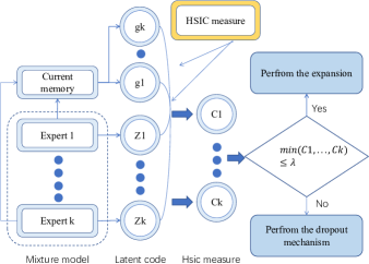
Fig. 1: Expansion and dropout mechanism in the proposed EMM model. We first infer the latent variables using each expert and then use HSIC to evaluate the discrepancy between each expert and the current memory. Then we perform either the mixture expansion or the memory buffer data dropout mechanism, according to the expansion criterion, Eq. (6).

3.3 Memory buffer data dropout mechanism

Since the memory buffer in the mixture model continually adds incoming samples, removing several stored samples from the memory buffer is necessary in order to keep the memory size in check. Let $|\mathcal{G}|^{max}$ represent the maximum number of samples in the memory. We introduce two simple dropout mechanisms to regularize the memory capacity. The first dropout mechanism, called EEM-SW, consists of using a sliding window successively removing the initially stored samples while adding new incoming samples in the memory buffer. The second dropout mechanism, called EEM-Random, randomly drops out sets of data samples from the memory buffer ${\mathcal{G}}_{j}$ at $\mathcal{T}_{j}$.

3.4 Implementation

The whole training procedure of the evolved mixture model can be divided into three main steps :

Step 1 (Training phase.)

At the training step ($\mathcal{T}_{j}$), the current memory ${\mathcal{G}}_{j-1}$ is updated to ${\mathcal{G}}_{j}={\mathcal{G}}_{j-1}\bigcup{\mathcal{D}}_{j}$. Then we train the current expert ($K$-th expert) on the memory buffer $\mathcal{G}_{j}$ using the loss function (Eq. (2) and Eq. (3)).

Step 2 (Checking the model’s expansion.)

In order to avoid frequently evaluating Eq. (6), we only check the model’s expansion when the current memory is full, $|{\mathcal{G}}_{j}|\geq|\mathcal{G}|^{max}$. To check the expansion, we calculate the HSIC measure between each expert and the data from the memory buffer, using Eq. (3.2). Then the mixture model will add a new expert if condition (6) is satisfied. For the new expert to learn statistically non-overlapping samples, we also clear up the current memory buffer ${\mathcal{G}}_{j}$ after the mixture’s expansion.

Step 3 (Dropout mechanism.)

This step aims to avoid memory overload. If the current memory buffer $\mathcal{G}_{j}$ at $\mathcal{T}_{j}$ is full, we drop out several samples (10 samples) from memory according to the dropout mechanism.

Table 1: Classification accuracy after five indepdnent runs for various models on three datasets. * and ${\dagger}$ denote the results cited from [7] and [25], respectively.

Methods	Split MNIST	Split CIFAR10	Split CIFAR100
iCARL*	83.95 $\pm$ 0.21	37.32 $\pm$ 2.66	10.80 $\pm$ 0.37
CoPE-CE*	91.77 $\pm$ 0.87	39.73 $\pm$ 2.26	18.33 $\pm$ 1.52
CoPE*	93.94 $\pm$ 0.20	48.92 $\pm$ 1.32	21.62 $\pm$ 0.69
ER + GMED†	82.67 $\pm$ 1.90	34.84 $\pm$ 2.20	20.93 $\pm$ 1.60
ERa + GMED†	82.21 $\pm$ 2.90	47.47 $\pm$ 3.20	19.60 $\pm$ 1.50
CURL*	92.59 $\pm$ 0.66	-	-
CNDPM*	93.23 $\pm$ 0.09	45.21 $\pm$ 0.18	20.10 $\pm$ 0.12
EEM-SW	96.79 $\pm$ 0.11	58.81 $\pm$ 0.12	22.33 $\pm$ 0.15
EEM-Random	96.73 $\pm$ 0.12	56.09 $\pm$ 0.15	21.78 $\pm$ 0.16

4 Experiments

4.1 Experiment setting

We consider the following TFCL benchmarks. Split MNIST and Split CIFAR10 splits MNIST [26] and CIFAR10 [27] into five tasks, respectively, where each task consists of samples from two classes. Split CIFAR100 divides CIFAR100 into 20 tasks and each task has 2500 examples from five classes.

Network architecture and hyperparameters for the classifier.

We adapt ResNet-18 [28] as the classifier used in Split CIFAR10 and Split CIFAR100 according to the setting from [7]. For Split MNIST, we adapt an MLP network, with 2 hidden layers with 400 units each [7], as the classifier. We set the maximum memory size for Split MNIST, Split CIFAR10, and Split CIFAR100 as 2000, 1000 and 5000, respectively. For each training step, a model only accesses a batch of 10 samples while all previous batches are not available.

4.2 Classification task

In Table 1 we evaluate EMM on Split MNIST, Split CIFAR10, and Split CIFAR100, and compare the results with several baselines including: Finetune which directly trains a classifier on the data stream, iCARL [29], CURL [22], CNDPM, CoPE [7], ER + GMED and ER_a + GMED [25], where GMED is Gradient based Memory Editing and ER is the experience replay [30], while ER_a is ER with data augmentation. The proposed approach outperforms not only single models such as CoPE, and GMED, but also the dynamic expansion model (CNDPM) on all three datasets.

Table 2: Classification accuracy for 20 runs for various models on Split MImageNet.

Methods	Split MImageNet	Permuted MNIST
ERa	25.92 $\pm$ 1.2	78.11 $\pm$ 0.7
ER + GMED	27.27 $\pm$ 1.8	78.86 $\pm$ 0.7
MIR+GMED	26.50 $\pm$ 1.3	79.25 $\pm$ 0.8
MIR	25.21 $\pm$ 2.2	79.13 $\pm$ 0.7
EEM-SW	28.90 $\pm$ 1.1	80.32 $\pm$ 0.6
EEM-Random	27.23 $\pm$ 1.2	80.28 $\pm$ 0.5

We also investigate the performance of various models on the large-scale dataset, MINI-ImageNet [31]. We split MINI-ImageNet into 20 disjoint subsets, where each subset contains samples from five classes [25], called Split MImageNet. We follow the setting from [25] where the maximum memory size is $10K$, and we implement the classifier of each expert by a slim version of ResNet-18 [28]. The results provided in Table 2, indicate that the proposed EEM outperforms all other methods under this challenging dataset, where the other methods results are cited from [25] and where MIR is the Maximally Interfered Retrieval.

4.3 Ablation study

We perform an ablation study to investigate the performance of the proposed EEM under different hyperparameter configurations. The performance and the model complexity for the EEM-SW model when varying the mixture expansion threshold $\lambda$ from Eq. (6) when training on Split MNIST are evaluated in Fig. 2. From Fig. 2-a, by increasing $\lambda$ leads to adding more components, but without necessary improving the classification accuracy when $\lambda$ is increased above a certain level, according to the results from Fig. 2-b.

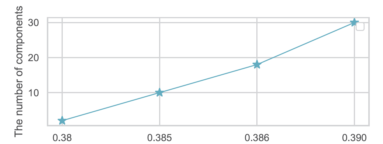
(a) No. of Components depending on the threshold $\lambda$

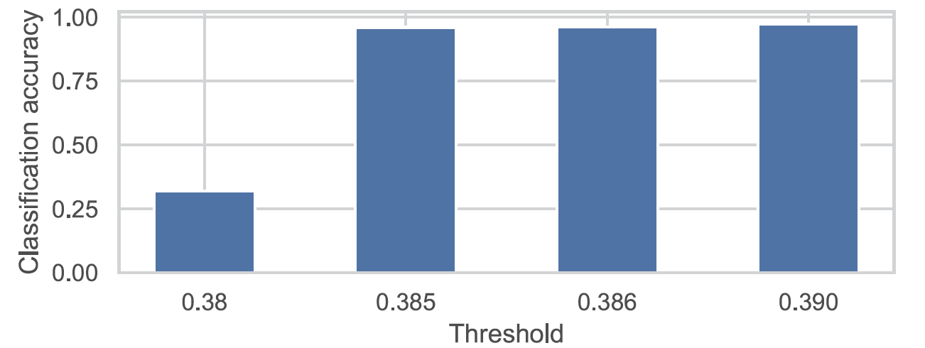
(b) Performance depending on the threshold $\lambda$

Fig. 2: Evaluation of the EMM-SW model when training on Split MNIST, when varying threshold $\lambda$ in Eq. (6).

5 Conclusion

In this paper, the Evolved Mixture Model (EMM) is proposed for learning infinite data streams without forgetting under the Task-Free Continual Learning (TFCL) setting. To address the data distribution shift in TFCL, we introduce a new mixture expansion mechanism based on the HSIC measure and also the selection of training. Finally, we perform experiments on several TFCL benchmarks, which show excellent results for the proposed approach.

References

- [1] G. I. Parisi, R. Kemker, J. L. Part, C. Kanan, and S. Wermter, “Continual lifelong learning with neural networks: A review,” Neural Networks, vol. 113, pp. 54–71, 2019.
- [2] Fei Ye and Adrian G. Bors, “InfoVAEGAN: Learning joint interpretable representations by information maximization and maximum likelihood,” in Proc. IEEE Int. Conf. on Image Processing (ICIP), 2021, pp. 749–753.
- [3] Fei Ye and Adrian G Bors, “Learning joint latent representations based on information maximization,” Information Sciences, vol. 567, pp. 216–236, 2021.
- [4] Fei Ye and Adrian G. Bors, “Learning latent representations across multiple data domains using lifelong VAEGAN,” in Proc. European Conf. on Computer Vision (ECCV), vol. LNCS 12365, 2020, pp. 777–795.
- [5] Fei Ye and Adrian G. Bors, “Lifelong learning of interpretable image representations,” in Proc. Int. Conf. on Image Processing Theory, Tools and Applications (IPTA), 2020, pp. 1–6.
- [6] Fei Ye and Adrian G. Bors, “Lifelong twin generative adversarial networks,” in Proc. IEEE Int. Conf. on Image Processing (ICIP), 2021, pp. 1289–1293.
- [7] Matthias De Lange and Tinne Tuytelaars, “Continual prototype evolution: Learning online from non-stationary data streams,” in Proc. of the IEEE/CVF Int. Conf. on Computer Vision (ICCV), 2021, pp. 8250–8259.
- [8] Heechul Jung, Jeongwoo Ju, Minju Jung, and Junmo Kim, “Less-forgetful learning for domain expansion in deep neural networks,” in Proc. of the AAAI Conf. on Artificial Intelligence, 2018, pp. 3358–3365.
- [9] Fei Ye and Adrian Bors, “Lifelong teacher-student network learning,” IEEE Transactions on Pattern Analysis and Machine Intelligence, pp. 1–18, 2021.
- [10] Fei Ye and Adrian G. Bors, “Lifelong infinite mixture model based on knowledge-driven Dirichlet process,” in Proc. of the IEEE Int. Conf. on Computer Vision (ICCV), 2021.
- [11] Fei Ye and Adrian G. Bors, “Lifelong mixture of variational autoencoders,” IEEE Transactions on Neural Networks and Learning Systems, pp. 1–14, 2021.
- [12] J. Kirkpatrick, R. Pascanu, N. Rabinowitz, J. Veness, G. Desjardins, A. A. Rusu, K. Milan, J. Quan, T. Ramalho, A. Grabska-Barwinska, D. Hassabis, C. Clopath, D. Kumaran, and R. Hadsell, “Overcoming catastrophic forgetting in neural networks,” Proc. of the National Academy of Sciences (PNAS), vol. 114, no. 13, pp. 3521–3526, 2017.
- [13] Arslan Chaudhry, Marc’Aurelio Ranzato, Marcus Rohrbach, and Mohamed Elhoseiny, “Efficient lifelong learning with A-GEM,” in Int. Conf. on Learning Representations (ICLR), arXiv preprint arXiv:1812.00420, 2019.
- [14] D. P. Kingma and M. Welling, “Auto-encoding variational Bayes,” arXiv preprint arXiv:1312.6114, 2013.
- [15] C. Cortes, X. Gonzalvo, V. Kuznetsov, M. Mohri, and S. Yang, “AdaNet: Adaptive structural learning of artificial neural networks,” in Proc. of Int. Conf. on Machine Learning (ICML), vol. PMLR 70, 2017, pp. 874–883.
- [16] Soochan Lee, Junsoo Ha, Dongsu Zhang, and Gunhee Kim, “A neural Dirichlet process mixture model for task-free continual learning,” in Proc. Int. Conf. on Learning Representations (ICLR), arXiv preprint arXiv:2001.00689, 2020.
- [17] Dushyant Rao, Francesco Visin, Andrei A. Rusu, Yee Whye Teh, Razvan Pascanu, and Raia Hadsell, “Continual unsupervised representation learning,” in Proc. Neural Inf. Proc. Systems (NeurIPS), 2019, pp. 7645–7655.
- [18] R. Aljundi, K. Kelchtermans, and T. Tuytelaars, “Task-free continual learning,” in Proc. od IEEE/CVF Conf. on Computer Vision and Pattern Recognition, 2019, pp. 11254–11263.
- [19] Fei Ye and Adrian G. Bors, “Deep mixture generative autoencoders,” IEEE Transactions on Neural Networks and Learning Systems, pp. 1–15, 2021.
- [20] Fei Ye and Adrian G Bors, “Mixtures of variational autoencoders,” in Proc. Int. Conf. on Image Processing Theory, Tools and Applications (IPTA), 2020, pp. 1–6.
- [21] Fei Ye and Adrian G Bors, “Lifelong generative modelling using dynamic expansion graph model,” in Proc. of the AAAI Conf. on Artificial Intelligence, 2022, vol. 36, pp. 1–9.
- [22] Dushyant Rao, Francesco Visin, Andrei Rusu, Razvan Pascanu, Yee Whye Teh, and Raia Hadsell, “Continual unsupervised representation learning,” in Advances in Neural Information Processing Systems (NeurIPS), 2019, pp. 7645–7655.
- [23] A. Gretton, O. Bousquet, A. Smola, and B. Schölkopf, “Measuring statistical dependence with Hilbert-Schmidt norms,” in Proc. Int. Conf. on Algorithmic Learning Theory, vol. Lecture Notes in Artif. Intell. (LNAI) 3734, 2005, pp. 63–77.
- [24] T. Wang and W. Li, “Kernel learning and optimization with Hilbert–Schmidt independence criterion,” Int. Jour. of Machine Learning and Cyber., vol. 9, no. 10, pp. 1707–1717, 2018.
- [25] Xisen Jin, Arka Sadhu, Junyi Du, and Xiang Ren, “Gradient-based editing of memory examples for online task-free continual learning,” in Advances in Neural Information Processing Systems (NeurIPS), 2021.
- [26] Y. LeCun, L. Bottou, Y. Bengio, and P. Haffner, “Gradient-based learning applied to document recognition,” Proc. of the IEEE, vol. 86, no. 11, pp. 2278–2324, 1998.
- [27] Alex Krizhevsky and Geoffrey Hinton, “Learning multiple layers of features from tiny images,” Tech. Rep., 2009.
- [28] K. He, X. Zhang, S. Ren, and J. Sun, “Deep residual learning for image recognition,” in Proc. of IEEE Conf. on Computer Vision and Pattern Recognition (CVPR), 2016, pp. 770–778.
- [29] Sylvestre-Alvise Rebuffi, Alexander Kolesnikov, Georg Sperl, and Christoph H Lampert, “iCaRL: Incremental classifier and representation learning,” in Proc. of IEEE Conf. on Computer Vision and Pattern Recognition (CVPR), 2017, pp. 2001–2010.
- [30] David Rolnick, Arun Ahuja, Jonathan Schwarz, Timothy P. Lillicrap, and Gregory Wayne, “Experience replay for continual learning,” in Advances in Neural Information Processing Systems (NeurIPS), 2019, pp. 348–358.
- [31] Ya Le and Xuan Yang, “Tiny ImageNet visual recognition challenge,” CS 231N, vol. 7, no. 7, pp. 3, 2015.