A search for compact object companions to high mass function single-lined spectroscopic binaries in Gaia DR3

Abstract

Gaia DR3 provides $>181,000$ radial velocity solutions for single-lined spectroscopic binaries (SB1s) which can be used to search for non-interacting compact object$+$star binary candidates by selecting systems with large mass functions. We selected 234 such systems and identified 115 systems with good RV solutions in DR3. We used light curves from ASAS-SN and TESS to identify and remove 31 eclipsing binaries to produce a catalog of 80 compact object+star candidates, including 38 ellipsoidal variables. The positions of these candidates on Gaia and 2MASS CMDs suggest that many of these systems are binaries with luminous companions. We compared the periods and eccentricities of detached eclipsing binaries in Gaia DR3 and ASAS-SN, and found that ${\sim}11\%$ and ${\sim}60\%$ of the binaries had different periods and eccentricities. We also compared RV solutions for 311 binaries in both Gaia DR3 and the Ninth Catalog of Spectroscopic Binary Orbits (SB9), and found similar results. We do not identify any strong candidates for non-interacting compact object+star binaries.

1 Introduction

The mass distribution of neutron stars and stellar mass black holes is closely tied to the evolution of massive stars, including their deaths (e.g., Pejcha & Thompson 2015; Sukhbold et al. 2016; Woosley et al. 2020). The relationship between the pre-supernova mass of the massive star and the type of compact remnant left behind is complex, and depends on the chemical composition of the star, mass-loss rates, supernova explosion physics and binary interactions (e.g., Sukhbold et al. 2016; Patton et al. 2021). While the fates of individual massive stars are hard to ascertain, we do know that dead massive stars leave behind a plethora of compact remnants in our Galaxy – there are predicted to be about ${\sim}10^{8}$ stellar mass BHs and ${\sim}10^{9}$ neutron stars in the Milky Way (e.g., Brown & Bethe 1994).

A well characterized, unbiased sample of neutron stars and black holes is necessary to better understand massive stars. However, this is a challenging task because the vast majority of compact objects are electromagnetically dark. To date, most mass measurements for neutron stars and black holes come from pulsar and accreting binary systems selected from radio, X-ray, and gamma-ray surveys (see, for e.g., Champion et al. 2008; Liu et al. 2006; Özel et al. 2010; Farr et al. 2011; Strader et al. 2015), and from the LIGO/Virgo detections of merging systems (see, for e.g., The LIGO Scientific Collaboration et al. 2021; Abbott et al. 2016, 2017). The populations of BHs observed as X-ray binaries and gravitational wave (GW) mergers are both heavily biased samples. In X-ray binaries, the companion must either fill its Roche lobe or have a modest separation and a strong stellar wind. Compact objects discovered through GW observations come from the small fraction of surviving binaries that are on very tight orbits leading to a merger. These interacting systems are, however, a small minority of compact object binaries, and the far larger population of non-interacting systems is essentially unexplored (Tanaka, 2002; Wiktorowicz et al., 2019). While non-interacting binaries are harder to find, they must be discovered and characterized in order to fully understand the numbers, properties, formation mechanisms, and evolutionary pathways of the interacting systems.

Rapid advances in time-domain astronomy (Shappee et al., 2014; Kochanek et al., 2017; Jayasinghe et al., 2018; Bellm et al., 2019; Tonry et al., 2018; Lindegren et al., 2021; Gaia Collaboration et al., 2022) provide promising pathways to discovering of non-interacting compact objects. For example, Chawla et al. (2021) estimated that ${\sim}30-300$ non-interacting black holes are detectable in binaries around luminous companions using Gaia astrometry. Similarly, Shao & Li (2019) used binary population synthesis models to estimate that there are thousands of non-interacting black holes in the Milky Way, with hundreds of these systems having luminous companions with $G<20$ mag. In addition to astrometry, targeted searches combining high-cadence photometry and sparsely sampled radial velocities from wide-field time-domain surveys are a promising method to discover more systems (e.g., Trimble & Thorne 1969; Thompson et al. 2019; Zheng et al. 2019; Rowan et al. 2021).

The discovery and confirmation of non-interacting compact objects is a challenging endeavour. As a result, only a handful of convincing non-interacting compact objects other than pulsars have been discovered thus far. Three non-interacting BH candidates have been discovered in globular clusters: one by Giesers et al. (2018) in NGC 3201 (minimum black hole mass $M_{\rm BH}=4.36\pm 0.41$ M_⊙), and two by Giesers et al. (2019) in NGC 3201 ($M_{\rm BH}\sin(i)=7.68\pm 0.50$ M_⊙ and $M_{\rm BH}\sin(i)=4.4\pm 2.8$ M_⊙). These globular cluster systems, if they indeed contain black holes, likely have formation mechanisms that are very different from those of field black hole binaries because the high stellar densities allow formation mechanisms which do not operate for field stars. A single convincing non-interacting BH candidate has been found in the field. Thompson et al. (2019) discovered a low-mass ($M_{\rm BH}\simeq 3.3_{-0.7}^{+2.8}~{}M_{\odot}$) non-interacting black hole candidate in the field on a circular orbit at $\rm P_{\rm orb}\sim 83\,d$ around a spotted giant star.

However, searches for non-interacting compact objects have also yielded numerous false positives. The binary LB-1 was initially thought to host an massive stellar black hole ($M_{\rm BH}\simeq 68_{-3}^{+11}~{}M_{\odot}$, Liu et al. 2019), but was later found to have a much less massive companion that was not necessarily a compact object (see, for e.g., Shenar et al. 2020; Irrgang et al. 2020; Abdul-Masih et al. 2020; El-Badry & Quataert 2020b). The naked-eye system HR 6819 was claimed to be a triple system with a detached black hole with $M_{\rm BH}=6.3\pm 0.7~{}M_{\odot}$ (Rivinius et al., 2020), but was later found to be a binary system with a rapidly rotating Be star and a slowly rotating B star (El-Badry & Quataert, 2020a; Bodensteiner et al., 2020). Recently, NGC 1850 BH1 was claimed to be a binary displaying ellipsoidal variability in the LMC with $M_{\rm BH}=11.1_{-2.4}^{+2.1}~{}M_{\odot}$ (Saracino et al., 2021), but was later argued to be a stripped B star binary (El-Badry & Burdge, 2021). Another example of a BH imposter was the system NGC 2004 #115, claimed to be a triple system consisting of a Be star on a tertiary orbit and an inner binary of a B star and a ${\simeq}25~{}M_{\odot}$ black hole (Lennon et al., 2021). El-Badry et al. (2021) later argued that the orbital inclination was underestimated by assuming tidal synchronization, and that the companion to the B star was more likely a ${\sim}2-3~{}M_{\odot}$ main sequence star. Jayasinghe et al. (2021) identified the nearby, nearly edge-on $\rm P_{\rm orb}=59.9$ d circular binary V723 Mon as a candidate for a compact object—star binary. El-Badry et al. (2022) later showed that V723 Mon is better explained by a stripped red giant in a binary around a massive (${\sim}2.8M_{\odot}$), rapidly rotating subgiant. A common theme to these cases is an overestimate of the mass of the observed star based on its luminosity and the assumption of single star evolution for a binary where mass transfer has greatly reduced the mass of the more luminous star.

Gaia DR3 (Gaia Collaboration et al., 2022; Babusiaux et al., 2022; Katz et al., 2022) provides a catalog of 181,529 single-lined spectroscopic binaries (SB1). However, it only provides the orbital solutions— the individual RV measurements will only be released in Gaia DR4. Nonetheless, these SB1 RV solutions are a useful starting point to search for non-interacting compact object+star binaries in the Milky Way. We describe the selection of high mass function binaries from the Gaia DR3 SB1 catalog, the vetting process that we used to discard false positives in Section 2 and compare the RV solutions for binaries in common between Gaia DR3 and the Rowan et al. (2022) catalog of detached eclipsing binaries or the SB9 catalog of spectroscopic binaries (Pourbaix et al., 2004). In Section 3, we discuss the vetted candidates. We present a summary of our results in Section 4.

2 Candidate Selection and Vetting using Gaia DR3

We describe the selection of single-lined spectroscopic binaries with high mass functions from Gaia DR3 and our vetting procedure to produce a catalog for the selection and follow-up of candidate non-interacting compact object binaries.

2.1 Selecting high mass function binaries from Gaia DR3

Figure 1 shows the distribution of the Gaia DR3 SB1 systems in orbital period, $f(M)$, eccentricity and the significance ($S$) of the RV solution. The median binary mass function is $f(M)\simeq~{}0.018~{}M_{\odot}$. Only ${\sim}0.07\%$ of the SB1s have $f(M)>1.5~{}M_{\odot}$. The distribution of orbital periods is more complicated, and it reflects the sampling of the Gaia survey as well as the true period distribution. However, the RV solutions are skewed towards longer periods— ${\sim}53\%$ of the DR3 SB1 solutions have an orbital period longer than 100 days. Most systems have modest orbital eccentricities, with a median eccentricity of $e_{\rm orb}\simeq 0.19$. Finally, ${\sim}40\%$ (${\sim}3\%$) of the SB1s have significance $S>20$ ($S>100$). For SB1s, the significance is the ratio of the RV semi-amplitude to its uncertainty. The median number of RV epochs used in DR3 is 23, but the RV solutions can have a minimum of 10 epochs or a maximum of 225 epochs, with ${\sim}1.4\%$ of the SB1s having more than 50 individual RV epochs.

Figure 2 shows the Gaia DR3 CMD for the ${\sim}181,000$ SB1s. We use distances from Bailer-Jones et al. (2021) and compute extinctions with the mwdust 3-dimensional ‘Combined19’ dust map (Bovy et al., 2016; Drimmel et al., 2003; Marshall et al., 2006; Green et al., 2019). We use Table 3 of Wang & Chen (2019) to convert the $A_{V}$ extinctions from mwdust to $A_{G}$ and $E(G_{\rm{BP}}-G_{\rm{RP}})$. We use isochrones from MESA Isochrones & Stellar Tracks (MIST, Choi et al., 2016; Dotter, 2016) to determine the evolutionary state of the candidates, following the prescription in Rowan et al. (2022). We interpolate over Solar metallicity MIST isochrones ranging in age from $10^{8}$ to $10^{10}$ years in intervals of $0.1$ in dex to define the boundary between main sequence stars and subgiants. To represent binary star isochrones in Figure 2, we double the flux in each band to represent an equal mass binary. The end of the subgiant branch is defined at the point when the radius is $R=1.5R_{\rm{TAMS}}$, where $R_{\rm{TAMS}}$ is the radius at the terminal age main sequence. We set the maximum absolute magnitude limit for the subgiant/giant branch to be $M_{G}=4.5$ mag. Of the ${\sim}181,000$ SB1s, ${\sim}95,000$, ${\sim}16,000$, and ${\sim}71,000$ are consistent with giants, sub-giants and main-sequence stars, respectively.

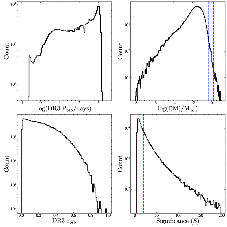
Figure 1: Distributions of the ${\sim}181,500$ Gaia DR3 SB1 systems in period, $f(M)$, eccentricity and the significance of the RV solution. In the mass function panel, the red and blue dashed lines show the selection limits for evolved and main sequence stars respectively. The dashed line in the significance panel shows the minimum significance we consider.

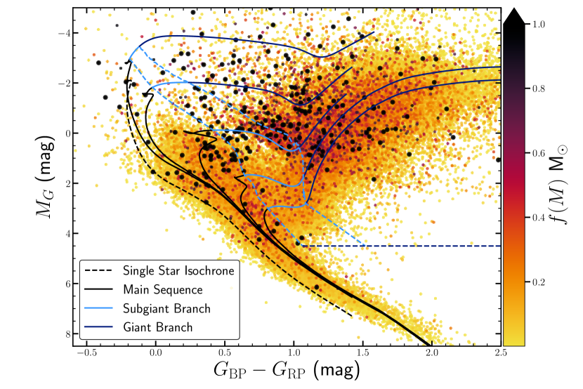
Figure 2: Gaia color-magnitude diagram for the ${\sim}181,000$ Gaia DR3 SB1 systems colored by their mass function, $f(M)$. Targets with $f(M)>1.0$ are shown as larger black points. Solar metallicity isochrones for equal mass binaries are shown as the solid lines for ages of $10^{8}$ to $10^{10}$ in intervals of 0.5 in dex, and divisions of the CMD from Rowan et al. (2022). The black dashed line shows a single star isochrone. The points are shaded by the binary mass function.

We select candidate SB1 systems based on their mass function

$$f(M)=\frac{P_{\rm orb}K^{3}(1-e^{2})^{3/2}}{2\pi G}=\frac{M_{\rm comp}^{3}\sin^{3}i}{(M_{\rm*}+M_{\rm comp})^{2}},$$ (1)

in the Gaia DR3 SB1 catalog. The binary mass function $f(M)$ is the minimum mass ($M_{\rm comp}$) of a companion in a spectroscopic binary in the limit where the mass of the observed star is $M_{\rm*}=0$ so the SB1 systems with high mass functions are good non-interacting compact object binary candidates. The best candidates for non-interacting black hole binaries are those with $f(M)>3~{}M_{\odot}$, as the minimum mass exceeds the maximum mass of a neutron star. We selected any system with $f(M)>1.5~{}M_{\odot}$ and main sequence systems with $f(M)>0.5~{}M_{\odot}$. The limit of $f(M)>1.5~{}M_{\odot}$ is to focus on NS and BH candidates. We use a higher threshold for the evolved stars because it is very difficult to estimate the stellar masses of evolved stars, while it is relatively easy to do so for main sequence stars. This yields 234 systems before any cuts on the significance.

Without the individual RVs for these systems, it is impossible to check the orbital solutions without new spectroscopic observations. For example, without adequate coverage of the maxima and minima in the RV curve, the semi-amplitude ($K$) and eccentricity ($e_{\rm orb}$) might be poorly constrained. In order to limit the false positives that may emerge from poor RV solutions in DR3, we use the significance ($S$) parameter in the SB1 catalog to sort our candidates into 4 categories. The best orbital solutions with $S\geq 100$ are assigned a grade of ‘A’, those with $50\leq S<100$ are assigned a grade of ’B’ and those with $20\leq S<50$ are assigned a grade of ’C’. The SB1 systems with $S<20$ are assigned a grade of ’D’ and are not considered further. The complete list of SB1s is available as supplementary information. There are 23, 24 and 68 SB1s with grades of A, B and C, respectively. There were 46 additional Grade D systems with $f(M)>1.5~{}M_{\odot}$. Figure 3 shows the distribution of period, $f(M)$ and the DR3 $G$-band magnitude for these systems. The median mass function is $f(M)\simeq 2.1~{}M_{\odot}$. There are 20 SB1 systems with $f(M)>3.0~{}M_{\odot}$. Not surprisingly given the properties of Gaia DR3, all of these high $f(M)$ SB1s are relatively bright ($G<14$ mag), and therefore suitable for ground-based radial velocity (RV) and other follow-up observations.

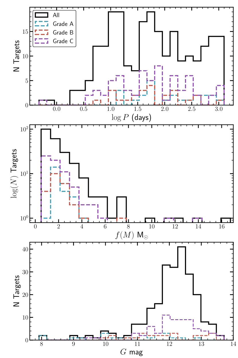
Figure 3: Distributions of the orbital period, mass function, and $G$ magnitude for the high mass function binaries.

2.2 Candidate Vetting

Here we describe the vetting process used to identify false positives for compact object–stellar binary systems. These include eclipsing binaries (EBs) and systems where the Gaia RV solutions are unlikely to be correct. Well-sampled light curves are needed to identify EBs. While Gaia DR3 comes with individual epoch photometry for ${\sim}10$ million variable stars (Eyer et al., 2022), not all of the SB1 systems have Gaia light curves and the Gaia light curves are generally sparse. Of the 115 A/B/C systems, only 45 had Gaia light curves in DR3. We instead use light curves from the All-Sky Automated Survey for SuperNovae (ASAS-SN; Shappee et al. 2014; Kochanek et al. 2017; Jayasinghe et al. 2018, Hart et al. in prep) and the Transiting Exoplanet Survey Satellite (TESS; Ricker et al. 2015) to identify EBs, ellipsoidal variables (ELLs), and systems where the Gaia period is inconsistent with the photometric period. We start by cross-matching our catalog with the ASAS-SN $V$- and $g$-band catalogs of variable stars (Jayasinghe et al., 2020; Christy et al., 2022) and find that a total of 33 targets (Grade A: 6, Grade B: 9, Grade C: 18) have been identified as photometric variables with classifications of EA, EB, EW, ROT, SR, VAR, and YSO. For the remaining targets, we compute $g$-band light curves using the ASAS-SN Sky Patrol (Kochanek et al., 2017). We also inspect the TESS light curves from the SPOC (Caldwell et al., 2020) and QLP (Huang et al., 2020a, b; Kunimoto et al., 2021) pipelines. Out of the 115 grade A-C targets, 102 have TESS light curves available for at least one sector. For both of these TESS pipelines we use the “raw” light curves rather than the detrended light curves because the detrending can remove real stellar variability.

In total, we identify 31 eclipsing binaries (Grade A: 7, Grade B: 9, Grade C: 15) that should not be further considered as candidates for hosting a compact object companion. We also identify 38 ellipsoidal variables (Grade A: 7, Grade B: 8, Grade C: 23). Figure 4 shows examples of an eclipsing binary, ellipsoidal, and ellipsoidal+eclipsing systems. We find that the TESS light curves are especially effective at identifying eclipsing ELL systems that may be missed in the ASAS-SN photometry because the higher photometric precision of the TESS data makes it more sensitive to shallow eclipses from a lower-luminosity companion star.

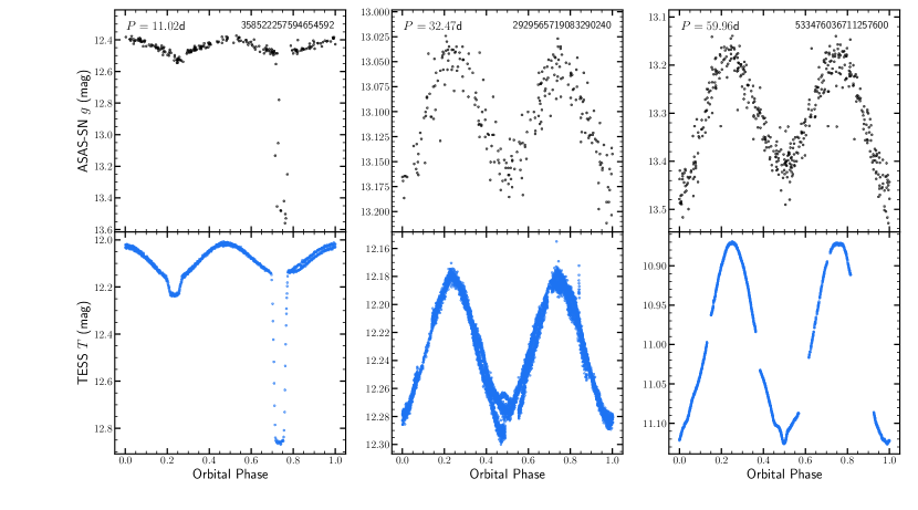
Figure 4: Examples of an eclipsing binary, an ellipsoidal variable, and an eclipsing ellipsoidal variable identified during candidate vetting. The top row shows the ASAS-SN $g$-band light curves and the bottom row shows TESS $T$ light curves. For the eclipsing binary, the orbit has been phased such that the primary eclipse occurs at phase 0.75. The ELL and ELL+ECL system have orbital phase defined such that the deeper minima occurs at phase 0.

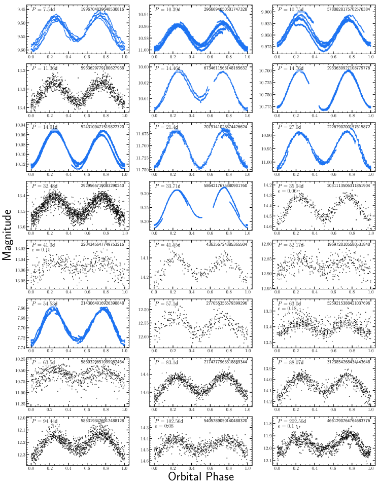
Figure 5: Examples of ellipsoidal variables identified in Section 2.2 from the ASAS-SN and TESS light curves. ASAS-SN light curves are shown in black and TESS light curves are shown in blue. The light curves have all been phased such that the deeper minimum occurs at phase zero. The photometric period is consistent with the Gaia RV period for all but four targets. These targets are removed from further consideration and not included here. The photometric period is given in the upper left of each panel, and the eccentricity from the Gaia SB1 solution is also shown for systems where $e>0.05$. The Gaia source ID is labeled in the upper right of each panel.

For the systems with ellipsoidal modulations we also verify that the photometric period is consistent with the Gaia RV period. We use a Generalized Lomb-Scargle (Lomb, 1976; Scargle, 1982) to identify the photometric period for targets not included in the ASAS-SN Variable Stars Database. Out of the 38, only 4 (10.5%) have photometric periods that are significantly different ($>10\%$) from the periods given in the Gaia SB1 solution:

• 6021285355771958528: $P_{\rm{Gaia}}=269.51$ d, $P_{\rm{LC}}=5.71$ d

• 5868858821883779328: $P_{\rm{Gaia}}=46.31$ d, $P_{\rm{LC}}=34.63$ d

• 878555832642451968: $P_{\rm{Gaia}}=837.10$ d, $P_{\rm{LC}}=8.39$ d

• 5543340020666175488: $P_{\rm{Gaia}}=135.75$ d, $P_{\rm{LC}}=20.91$ d

Without access to the individual epochs of Gaia RVs, we are unable to independently fit the RV curve and obtain the correct mass function, so these systems are removed from further consideration. Similarly, the presence of ellipsoidal variability can be used to evaluate the eccentricity reported in the SB1 fit. All of the targets identified as ellipsoidal variables have light curves consistent with zero eccentricity, yet 12 systems have $e>0.05$ from the Gaia SB1 fit. Figure 5 shows some of the grade A-C ellipsoidal variables that have consistent photometric and spectroscopic periods. Out of the 31 eclipsing binaries identified during the vetting, 13 (41.9%) have photometric periods that differ by $>10\%$ from the Gaia SB1 solution.

These period differences, where we would generally expect them to be the same since the photometric variability is also dominated by the brighter star, suggested doing a broader examination of the SB1 solutions. We cross matched the SB1 catalog to the Rowan et al. (2022) catalog of detached eclipsing binaries and the SB9 (Pourbaix et al., 2004) catalog of spectroscopic binaries. We identified 596 spectroscopic binaries in common between Gaia DR3 and the ASAS-SN detached binaries. Figure 6 shows comparisons of the orbital periods and eccentricities for these detached binaries. Of the 596 systems, ${\sim}89\%$ had periods that agreed to within $\pm 10\%$ and ${\sim}40\%$ had eccentricities that agreed to within 0.05. The median fractional error in the DR3 period and the median error in the eccentricity for these detached binaries is ${\sim}0.005\%$ and ${\sim}0.028$ respectively. If we only select the 245 systems that have $S>20$ in Gaia DR3, ${\sim}94\%$, and ${\sim}59\%$ had periods, and eccentricities that agreed to within these levels. While most of the binaries have periods that agree, the Gaia DR3 eccentricities for many circular systems are overestimated.

We identified 311 spectroscopic binaries in common between Gaia DR3 and SB9. Of the 311 systems, 12 systems (${\sim}4\%$) were cataloged as double-lined spectroscopic binaries (SB2) in the SB9 catalog and 245 of these systems (${\sim}79\%$) have $S>20$ in Gaia DR3. The median Gaia DR3 G-band magnitude for these SB1s is ${\sim}8.2$ mag. Figure 6 also shows comparisons of the orbital periods, RV semi-amplitudes and eccentricities for these SB1 systems. The median fractional error in the DR3 period and the median error in the eccentricity for these systems is ${\sim}0.1\%$ and ${\sim}0.016$ respectively. Of the 311 systems, ${\sim}85\%$, ${\sim}80\%$ had periods and semi-amplitudes that agreed to within $\pm 10\%$ and ${\sim}70\%$ had eccentricities that agreed to within 0.05. If we only select the 245 systems that have $S>20$ in Gaia DR3, ${\sim}94\%$, ${\sim}90\%$ and ${\sim}81\%$ had periods, semi-amplitudes and eccentricities that agreed to within these levels. These comparisons support the use of $S>20$ to select for good RV solutions. The agreement in period and semi-amplitude is generally very good for orbital periods shorter than ${\sim}1000$ days. The level of agreement on the eccentricity is significantly worse, which is not surprising given the typical numbers of RV measurements going into the orbital solutions.

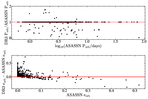
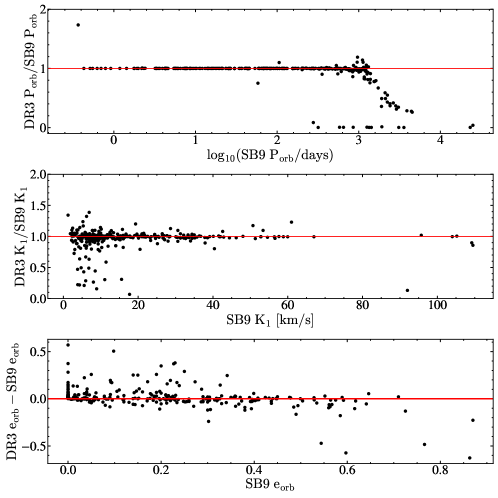
Figure 6: The top two panels compare the Gaia DR3 and ASAS-SN eclipsing binary periods (upper) and eccentricities (lower). The bottom three panels compare the Gaia DR3 and SB9 spectroscopic binary periods (upper), RV semi-amplitudes (middle) and eccentricities (lower). The red lines correspond to a one-to-one agreement between both catalogs. Aside from the very long period systems, the agreement in period and semi-amplitude is generally good, but there is significant scatter in the eccentricities.

3 Discussion

Table 1: The vetted catalog of Gaia DR3 SB1s for Grades A and B. Grade C targets are shown in Table 2. Targets are sorted by $f(M)$. The ‘remarks’ column labels the systems identified here as ELLs, the classification given in the ASAS-SN $V$- and $g$-band variable stars catalogs, and systems with HI features near 860 nm.

Gaia DR3 Source ID	TIC	$G$	N RVs	Significance	RV Ecc	RV Period	$K_{1}$	$f(M)$	Remarks
		(mag)				(d)	(km/s)	M⊙
Grade A:
206292746724589824	65919311	$11.567327$	15	$134.814390$	$0.027971$	$347.001862$	$50.101911$	$4.516898$	SR
5869320651099982464	443204265	$9.878837$	13	$257.181240$	$0.014177$	$63.923918$	$77.526747$	$3.085621$	ELL
5864217675880901760	319384609	$9.307944$	23	$276.200960$	$0.006531$	$32.957533$	$94.372047$	$2.870202$	ELL
5853193426917488128	397891772	$11.231160$	58	$187.938600$	$0.027227$	$94.546816$	$64.570534$	$2.634646$	ELL, SR
2021374066702077312	113100455	$10.040213$	16	$249.071850$	$0.007008$	$44.413183$	$80.354996$	$2.387668$	HI
2008602689332951808	433877616	$11.561862$	19	$176.193630$	$0.087776$	$746.780507$	$29.567067$	$1.977127$
426648861352371328	256101165	$11.765608$	30	$198.133480$	$0.008147$	$240.418458$	$42.286516$	$1.883587$
277055356579399296	9133993	$11.498751$	19	$139.798610$	$0.013096$	$57.082604$	$68.054182$	$1.863854$	ELL
5541400855806539392	182220071	$12.323505$	28	$120.971080$	$0.076998$	$680.690124$	$29.852769$	$1.859881$
6734611563148165632	405124480	$10.940159$	10	$106.440285$	$0.008308$	$14.344372$	$104.398021$	$1.691098$	ELL, EB22
5352456452682656256	457864395	$12.029145$	27	$126.030106$	$0.020771$	$59.850214$	$64.053421$	$1.628797$	HI
510691269572063232	54722608	$11.950563$	25	$111.722220$	$0.278042$	$401.907835$	$34.902305$	$1.569386$
5243109471519822720	371686230	$10.451161$	22	$170.075780$	$0.022729$	$14.913679$	$100.370249$	$1.561416$	ELL, EB22, HI
2143064916926398848	243276811	$7.970002$	20	$331.717400$	$0.004292$	$54.130368$	$65.181678$	$1.553320$	ELL
4061400381769067392	198141489	$7.919531$	12	$343.417570$	$0.005649$	$619.989392$	$28.622871$	$1.506463$
5722942457613931264	386429851	$9.942932$	16	$114.958830$	$0.024770$	$38.099937$	$65.575140$	$1.112153$
Grade B:
527155253604491392	444463982	$13.241814$	18	$56.404236$	$0.039641$	$149.155050$	$58.748022$	$3.126430$
5934549483335296384	8390898	$13.336455$	23	$66.629875$	$0.011894$	$39.459315$	$83.878903$	$2.412520$
1969720105580531840	273409875	$11.867422$	20	$71.996254$	$0.029184$	$52.245971$	$75.034792$	$2.284237$	ELL
436356724385365504	117261905	$13.116592$	20	$74.995186$	$0.046568$	$41.667586$	$79.763055$	$2.183961$	ELL, YSO
4116115997318757120	351790283	$10.605717$	11	$80.141230$	$0.219198$	$41.298015$	$78.581979$	$1.928752$
2226790700157615872	376968598	$11.620328$	20	$58.101974$	$0.029358$	$26.896792$	$88.313918$	$1.917263$	ELL, YSO, HI
5405789050140488320	432646925	$13.239762$	25	$50.698112$	$0.075597$	$102.598820$	$56.378678$	$1.888899$	ELL, SR
461251282546634496	251656921	$12.900666$	22	$78.366120$	$0.012467$	$457.299371$	$33.544210$	$1.788164$
6054973670507378944	450908863	$12.814929$	16	$83.004320$	$0.014411$	$127.955769$	$51.231189$	$1.782310$
2079141028874426624	268608966	$12.101652$	19	$68.671630$	$0.005746$	$21.581811$	$88.101534$	$1.529228$	ELL
6019286920341931520	458320995	$11.687070$	27	$53.460700$	$0.048750$	$47.562497$	$67.450289$	$1.507028$
2933630927108779776	79033600	$11.067193$	20	$68.974550$	$0.021142$	$14.717528$	$92.918559$	$1.222569$	ELL, EB22
2966694650501747328	33520660	$11.203405$	31	$79.496640$	$0.019488$	$10.397987$	$102.373299$	$1.155272$	ELL, EB22
5780828175702576384	324759352	$10.235976$	19	$80.753044$	$0.048828$	$10.749564$	$84.845983$	$0.677879$	ELL
3102189152022476288	36344278	$11.962961$	10	$53.590000$	$0.152794$	$6.085486$	$103.485478$	$0.674477$

• The remark EB22 means the system was included in El-Badry & Rix (2022).

Table 2: Same as 1 but for Grade C targets.

Gaia DR3 Source ID	TIC	$G$	N RVs	Significance	RV Ecc	RV Period	$K_{1}$	$f(M)$	Remarks
		(mag)				(d)	(km/s)	M⊙
Grade C:
4661290764764683776	31181424	$11.770099$	13	$29.410261$	$0.095333$	$204.929896$	$86.675141$	$13.639446$	ELL
5259215388421037696	274794828	$12.212911$	27	$42.088013$	$0.183672$	$62.706640$	$123.079353$	$11.507172$	ELL
2006840790676091776	388220893	$11.183457$	13	$28.334784$	$0.203377$	$4.073262$	$239.758434$	$5.460109$
442992311418593664	117801951	$9.551256$	20	$21.781998$	$0.413849$	$216.530553$	$65.532625$	$4.763938$
2174777963318889344	260523268	$13.064586$	23	$31.486582$	$0.023252$	$82.722662$	$76.398430$	$3.819275$	ELL
2031113506311851904	105414150	$13.237762$	22	$41.551937$	$0.057142$	$35.908104$	$100.607380$	$3.770568$	ELL
1996704839648530816	323630694	$9.797777$	17	$38.942818$	$0.046335$	$7.545741$	$168.690275$	$3.741341$	ELL
251157906379754496	428692810	$12.054820$	21	$49.165646$	$0.088727$	$296.675772$	$49.153139$	$3.607800$
3331748140308820352	438063379	$12.716515$	13	$41.455563$	$0.066978$	$225.268159$	$53.484464$	$3.547392$
5963629779180627968	123810745	$11.818235$	13	$25.285658$	$0.029502$	$11.368877$	$139.363823$	$3.184607$	ELL, EA
2929565719083290240	81733775	$12.877993$	28	$49.930740$	$0.033133$	$32.473360$	$97.134994$	$3.078891$	ELL, EB
5596083868330026624	152577827	$11.313450$	30	$29.111685$	$0.016003$	$57.846818$	$78.531008$	$2.901961$	HI
5545731836408967040	419154174	$12.634378$	23	$24.275116$	$0.013377$	$983.518197$	$29.538204$	$2.625871$
3123854268434443648	234801497	$12.635286$	10	$46.279648$	$0.032723$	$87.885426$	$64.503233$	$2.440163$	ELL
2170359438392059776	267479007	$13.284603$	28	$39.155950$	$0.066104$	$49.274869$	$77.844395$	$2.392820$
2208323856913151360	12871969	$12.969639$	21	$27.721788$	$0.062588$	$84.991016$	$64.424862$	$2.341165$
440218930776209664	116842332	$13.042632$	25	$27.773575$	$0.182453$	$47.537018$	$78.616544$	$2.274962$
2004074312033531264	389024325	$12.771193$	18	$32.358902$	$0.431375$	$1117.916540$	$29.162925$	$2.109731$
5866096676853138432	330567799	$11.415991$	32	$23.974285$	$0.083211$	$76.373014$	$63.171280$	$1.974368$
2204345647749753216	411042914	$12.717619$	25	$28.429789$	$0.145334$	$41.268379$	$77.860137$	$1.954839$	ELL, HI
3401898906303342848	6240885	$12.385528$	20	$24.790207$	$0.142666$	$35.665994$	$78.726311$	$1.748532$	ELL, ROT, HI
5877107564251430400	45246020	$13.712082$	25	$28.775150$	$0.229085$	$925.166866$	$26.935992$	$1.728053$
427039394137929216	420024388	$11.398898$	25	$24.639140$	$0.078857$	$5.436449$	$145.160304$	$1.707068$	ELL, VAR
5694373091078326784	155728890	$11.913286$	24	$30.750462$	$0.017614$	$12.884807$	$107.469851$	$1.656499$	EB22
4514813786980451840	451659136	$12.565736$	18	$24.562475$	$0.136061$	$22.020434$	$88.831086$	$1.555261$	EB22
5325390221595083520	400862980	$13.442926$	21	$23.994865$	$0.338450$	$381.859396$	$36.053700$	$1.545096$
5529029223988702976	181003751	$10.852627$	20	$39.660534$	$0.096665$	$141.361843$	$47.405253$	$1.538690$
4657646364721058304	404851003	$10.861196$	13	$24.140335$	$0.052787$	$272.685820$	$37.752778$	$1.514074$
948585824160038912	9961832	$11.956474$	10	$21.798958$	$0.077334$	$8.201945$	$120.352267$	$1.468230$	ELL, EB22
2219809419798508544	372337574	$12.480452$	17	$38.396572$	$0.074999$	$10.865285$	$104.787932$	$1.284466$	ELL, ROT, EB22
5536105058044762240	123110322	$12.154784$	11	$24.045340$	$0.085800$	$12.176559$	$98.074715$	$1.177076$	ELL, EB22
4239611700214875904	95324628	$11.914187$	17	$23.599092$	$0.404139$	$56.124101$	$62.948652$	$1.110104$
4341334461557059328	157778582	$13.509942$	18	$21.707628$	$0.379624$	$353.710453$	$33.458745$	$1.086982$
3107879743172451456	177622520	$11.904951$	10	$21.314194$	$0.026828$	$27.304940$	$72.539931$	$1.078762$
5610703902634458112	63361138	$11.006958$	37	$48.140770$	$0.021076$	$1003.250050$	$21.017484$	$0.964460$
4295254307232999296	135660189	$11.553295$	16	$29.559841$	$0.046062$	$10.832797$	$93.256394$	$0.907434$	ELL, EB
209136938490844928	369256285	$12.401679$	21	$30.389870$	$0.042916$	$14.291517$	$83.789328$	$0.868692$	ELL, HI
6551893071549223040	175399204	$11.893268$	12	$36.334988$	$0.092529$	$79.395211$	$46.970404$	$0.841566$
5558841347897409408	130374599	$11.852222$	27	$49.228947$	$0.067814$	$12.819832$	$84.129925$	$0.785513$	ELL
6609971199873698944	47505992	$11.518994$	12	$36.472637$	$0.193909$	$18.342281$	$75.658301$	$0.777103$
5337295389939374592	466883848	$13.003701$	14	$27.571960$	$0.013766$	$274.397225$	$29.961135$	$0.764457$
4278307358382586880	168891318	$12.534010$	10	$29.479143$	$0.174147$	$11.962745$	$84.255175$	$0.707914$
5461264982333157888	71585696	$12.305203$	55	$21.673530$	$0.316210$	$762.774486$	$21.407609$	$0.662056$
4039283116865495424	58882119	$11.994610$	15	$20.938140$	$0.127662$	$79.548781$	$43.365410$	$0.655816$
6475655404885617920	100475949	$12.372097$	15	$20.482758$	$0.101280$	$46.094713$	$51.414310$	$0.639159$
4345739070777246080	135817331	$12.287071$	13	$29.691814$	$0.095857$	$6.195072$	$97.469449$	$0.586220$	ELL, ROT
5834976099807482752	428137933	$12.196315$	22	$21.362688$	$0.046363$	$39.265479$	$52.202597$	$0.576909$
421738201900868608	449984714	$11.459711$	27	$33.416725$	$0.037187$	$16.552523$	$68.819819$	$0.557860$	ELL
2220072241734878720	372137170	$11.751909$	14	$21.381530$	$0.179089$	$331.191043$	$24.850305$	$0.501488$

• The remark EB22 means the system was included in El-Badry & Rix (2022).

After the vetting in $\S$2.2, we are left with the 80 candidates in Tables 1 and 2. While some of these may represent good targets for spectroscopic follow-up to identify non-interacting compact objects, further analysis of the spectral energy distributions (including the low resolution Gaia $BP/RP$ spectra) and their positions on the color-magnitude diagram (CMD) should be used to search for signs of a luminous companion and identify the best candidates for follow-up observations.

Figure 7 shows the Grade A/B/C targets on Gaia and 2MASS CMDs after correcting for extinction. Solar metallicity isochrones where the flux in each band has been doubled to represent an equal mass binary are also shown. The divisions into evolutionary states shown by the colored dashed lines are described in $\S 2.1$. Of the 80 candidates in Tables 1 and 2, 31, 15 and 34 are main sequence stars, sub giants and red giants in the Gaia DR3 CMD, respectively. In the 2MASS CMD, there were 14, 19 and 47 main sequence stars, sub giants and red giants, respectively. Of the 80 vetted candidates, only 51 had matching evolutionary states in both the Gaia and 2MASS CMDs.

On the Gaia CMD, the majority of the vetted systems are found in the Hertzsprung gap where few stars should dwell. This likely indicates the presence of a luminous companion instead of a dark compact object, where the intermediate $G_{\rm BP}-G_{\rm RP}$ colors are created by blending the spectral energy distributions (SEDs) of a cooler/redder star and a hotter/bluer star. When the same systems are examined on the 2MASS CMD, most of these systems now lie closer to the red giant branch, which supports the idea that a large number of these vetted systems are stellar binaries. Indeed, 12 of our targets were also investigated by El-Badry & Rix (2022) who argue that these are mass-transfer binaries consisting of a stripped giant with $M<0.5$ M_⊙ and a blue companion. We highlight the systems that are in the El-Badry & Rix (2022) catalog with black outlines on Figure 7 and label them in Table 1.

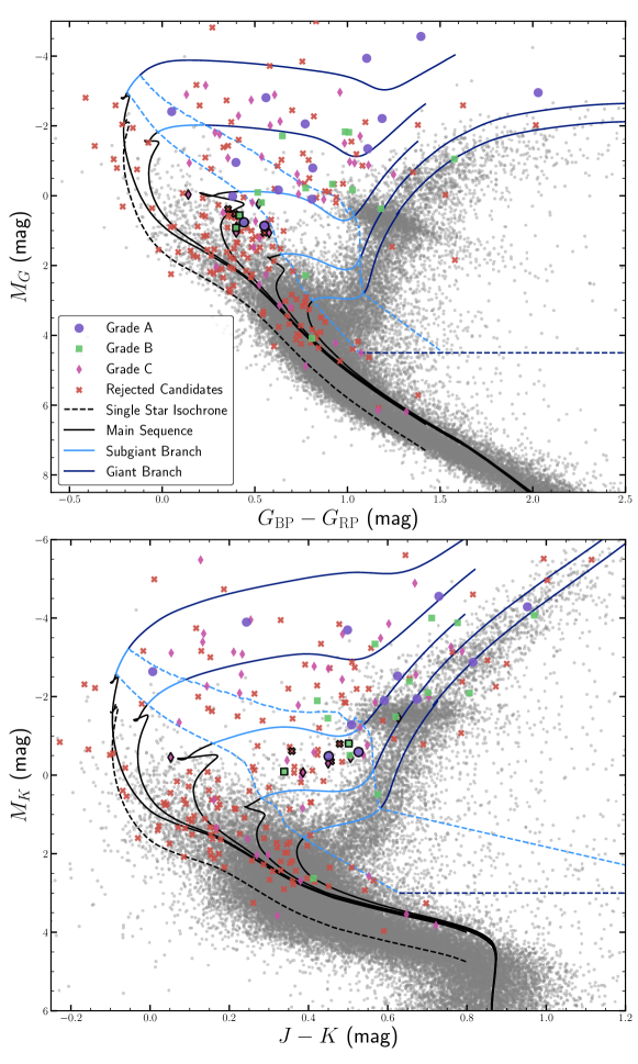
Figure 7: Gaia (top) and 2MASS (bottom) color-magnitude diagram for the high mass function SB1 systems. The gray background shows a random selection of Gaia targets. The colored points show the Grade A, B, and C systems that remain after light curve inspection. The black crosses mark systems that were rejected based on the significance cut ($S<20$) or the light curves. Isochrones for equal mass binaries are shown as the solid lines, and divisions of the CMD from Rowan et al. (2022). The black dashed line shows a single star isochrone.

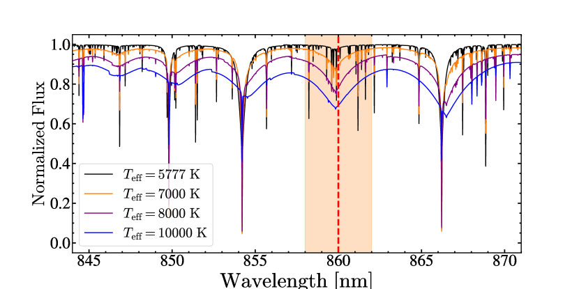
Figure 8: Synthetic spectra in the wavelength range covered by the Gaia RVS spectrometer for main sequence stars with various $T_{\rm eff}$. The red dashed line and the orange shaded region shows the position of the H I absorption feature that is sensitive to $T_{\rm eff}$.

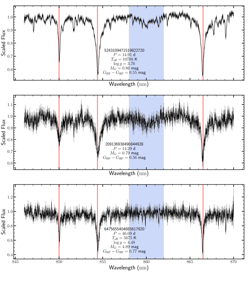
Figure 9: Mean Gaia RVS spectra for three main sequence targets. The top panel shows 5243109471519822720, a mass transfer system identified in El-Badry & Rix (2022). The middle panel shows one of our candidates with a similar spectrum, suggesting that it is also a binary with a hot accretor and cool donor star. The bottom shows a candidate with a spectrum that is more consistent with what is expected from a single star. In each panel, the Gaia Source ID, period, and extinction-corrected absolute magnitude and color are shown. For the first and third targets, estimates of the effective temperature and surface gravity are given from Gaia-Flame. In each panel, the red lines show Ca I lines, and the blue shaded region shows a H I line that is sensitive to $T_{\rm eff}$.

Although the individual spectra are not available for each RV epoch, mean Gaia RVS spectra with $R{\sim}11,500$ are available for 66 of the 234 targets (${\sim}28\%$). While the RVS spectra only span a limited range in wavelength (${\sim}845-871$ nm), they can be used to identify double-lined spectroscopic binaries. In particular, El-Badry et al. (2022) point out that the H I absorption feature in the RVS spectra at 860 nm is sensitive to the effective temperature. It is only present for $T_{eff}\gtrsim 7000$ K and then has an equivalent width that increases with temperature. Figure 9 shows RVS spectra for three targets on our vetted list. The top panel shows 5243109471519822720, which is one of potential the mass-transfer systems from El-Badry et al. (2022) (their Figure 2) and the broad H I feature lies in the shaded band. We examined the 11 available RVS spectra for the 39 targets classified as red giants in the 2MASS CMD (Figure 7). We found that 6 of the 11 targets had evidence of this feature and so are likely stellar binaries with a red giant and a hotter stellar component. These systems are flagged with an ‘HI’ in Tables 1 and 2.

The Gaia DR3 APSIS/MSC module (Fouesneau et al. 2022) models each system’s $BP/RP$ spectrum as two stars in order to search for unresolved binaries. This seemed an obvious way to identify stellar binaries with very different temperatures. Unfortunately, the solutions are almost all reported to have very low posterior probabilities. Figure 10 shows the two MSC temperatures coded by the posterior probabilities. Fouesneau et al. (2022) note that the interpretation of the posteriors is presently not fully understood, but in comparisons to known GALAH unresolved binaries, the temperature differences rise from 135 K (258 K) for the primary (secondary) for the stars in the top 5% of the posterior distribution, to 387 K (632 K) for those in the bottom 5%. Bear in mind that if the systems in the Hertzsprung gap are due to combining a giant and a MS star, the temperature differences should be very large. Of the 79 vetted candidates, there were 24 that had $\Delta T_{\rm eff}>1000$ K. Of the 24 systems with $\Delta T_{\rm eff}>1000$ K, 13 were identified as sub giants or red giants in the Gaia CMD (Figure 7). This also suggests that some of these systems are in fact stellar binaries with a blended SED.

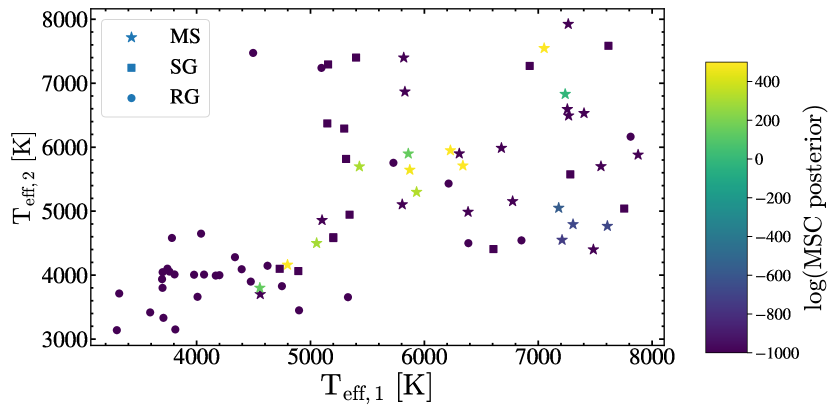
Figure 10: Comparison of the reported $T_{\rm eff}$ (primary and secondary) in the Gaia DR3 APSIS/MSC module for the 80 candidates in Tables 1 and 2.

4 Conclusions

Gaia DR3 provides $>181,000$ radial velocity solutions for single-lined spectroscopic binaries. We selected 234 SB1s with binary mass functions $f(M)>1.5~{}M_{\odot}$ (evolved) or $f(M)>0.5~{}M_{\odot}$ (main sequence) and identified 115 systems with good RV solutions ($S>20$) in Gaia DR3. Using light curves from ASAS-SN and TESS, we vet the selected SB1s to remove false positives from eclipsing binaries. We identified 31 eclipsing binaries and 38 ellipsoidal variables. We produced a catalog of 80 vetted SB1 candidates. The positions of the vetted SB1 candidates on the Gaia and 2MASS CMDs suggest that many, if not all, of these systems are binaries with luminous companions. We do not find any strong candidates for non-interacting compact object+star binaries with just the Gaia, ASAS-SN and TESS data. Further spectroscopic follow-up is necessary to determine whether these systems are non-interacting compact object binaries.

After noting some discrepancies between the Gaia periods for the eclipsing binaries and ellipsoidal variables we identified among the candidates, we did a broader comparison using the 596 detached eclipsing binaries from Rowan et al. (2022) and the 311 spectroscopic SB9 (Pourbaix et al. 2004) binaries that had SB1 solutions. For the eclipsing binaries, ${\sim}89\%$ had periods that agreed to within $\pm 10\%$ and ${\sim}40\%$ had eccentricities that agreed to within 0.05. For the spectroscopic binaries, we found that ${\sim}85\%$, ${\sim}80\%$ of these systems had periods and semi-amplitudes that agreed to within $\pm 10\%$. However, only ${\sim}70\%$ of these systems had eccentricities that agreed to within 0.05.

Data Availability

The Gaia DR3 data, the ASAS-SN and TESS light curves are all publicly available.

References

- Abbott et al. (2016) Abbott B. P., et al., 2016, Phys. Rev. Lett., 116, 061102
- Abbott et al. (2017) Abbott B. P., et al., 2017, Phys. Rev. Lett., 119, 161101
- Abdul-Masih et al. (2020) Abdul-Masih M., et al., 2020, Nature, 580, E11
- Babusiaux et al. (2022) Babusiaux C., et al., 2022, arXiv e-prints, p. arXiv:2206.05989
- Bailer-Jones et al. (2021) Bailer-Jones C. A. L., Rybizki J., Fouesneau M., Demleitner M., Andrae R., 2021, AJ, 161, 147
- Bellm et al. (2019) Bellm E. C., et al., 2019, PASP, 131, 018002
- Bodensteiner et al. (2020) Bodensteiner J., et al., 2020, A&A, 641, A43
- Bovy et al. (2016) Bovy J., Rix H.-W., Green G. M., Schlafly E. F., Finkbeiner D. P., 2016, ApJ, 818, 130
- Brown & Bethe (1994) Brown G. E., Bethe H. A., 1994, ApJ, 423, 659
- Caldwell et al. (2020) Caldwell D. A., et al., 2020, Research Notes of the American Astronomical Society, 4, 201
- Champion et al. (2008) Champion D. J., et al., 2008, Science, 320, 1309
- Chawla et al. (2021) Chawla C., Chatterjee S., Breivik K., Krishna Moorthy C., Andrews J. J., Sanderson R. E., 2021, arXiv e-prints, p. arXiv:2110.05979
- Choi et al. (2016) Choi J., Dotter A., Conroy C., Cantiello M., Paxton B., Johnson B. D., 2016, ApJ, 823, 102
- Christy et al. (2022) Christy C. T., et al., 2022, arXiv e-prints, p. arXiv:2205.02239
- Dotter (2016) Dotter A., 2016, ApJS, 222, 8
- Drimmel et al. (2003) Drimmel R., Cabrera-Lavers A., López-Corredoira M., 2003, A&A, 409, 205
- El-Badry & Burdge (2021) El-Badry K., Burdge K., 2021, arXiv e-prints, p. arXiv:2111.07925
- El-Badry & Quataert (2020a) El-Badry K., Quataert E., 2020a, arXiv e-prints, p. arXiv:2006.11974
- El-Badry & Quataert (2020b) El-Badry K., Quataert E., 2020b, MNRAS, 493, L22
- El-Badry & Rix (2022) El-Badry K., Rix H.-W., 2022, arXiv e-prints, p. arXiv:2206.07723
- El-Badry et al. (2021) El-Badry K., Burdge K. B., Mróz P., 2021, arXiv e-prints, p. arXiv:2112.05030
- El-Badry et al. (2022) El-Badry K., Seeburger R., Jayasinghe T., Rix H.-W., Almada S., Conroy C., Price-Whelan A. M., Burdge K., 2022, arXiv e-prints, p. arXiv:2203.06348
- Eyer et al. (2022) Eyer L., et al., 2022, arXiv e-prints, p. arXiv:2206.06416
- Farr et al. (2011) Farr W. M., Sravan N., Cantrell A., Kreidberg L., Bailyn C. D., Mandel I., Kalogera V., 2011, ApJ, 741, 103
- Fouesneau et al. (2022) Fouesneau M., et al., 2022, arXiv e-prints, p. arXiv:2206.05992
- Gaia Collaboration et al. (2022) Gaia Collaboration et al., 2022, arXiv e-prints, p. arXiv:2206.05595
- Giesers et al. (2018) Giesers B., et al., 2018, MNRAS, 475, L15
- Giesers et al. (2019) Giesers B., et al., 2019, A&A, 632, A3
- Green et al. (2019) Green G. M., Schlafly E., Zucker C., Speagle J. S., Finkbeiner D., 2019, ApJ, 887, 93
- Huang et al. (2020a) Huang C. X., et al., 2020a, Research Notes of the American Astronomical Society, 4, 204
- Huang et al. (2020b) Huang C. X., et al., 2020b, Research Notes of the American Astronomical Society, 4, 206
- Irrgang et al. (2020) Irrgang A., Geier S., Kreuzer S., Pelisoli I., Heber U., 2020, A&A, 633, L5
- Jayasinghe et al. (2018) Jayasinghe T., et al., 2018, MNRAS, 477, 3145
- Jayasinghe et al. (2020) Jayasinghe T., et al., 2020, arXiv e-prints, p. arXiv:2006.10057
- Jayasinghe et al. (2021) Jayasinghe T., et al., 2021, MNRAS, 504, 2577
- Katz et al. (2022) Katz D., et al., 2022, arXiv e-prints, p. arXiv:2206.05902
- Kochanek et al. (2017) Kochanek C. S., et al., 2017, PASP, 129, 104502
- Kunimoto et al. (2021) Kunimoto M., et al., 2021, Research Notes of the American Astronomical Society, 5, 234
- Lennon et al. (2021) Lennon D. J., Dufton P. L., Villaseñor J. I., Evans C. J., Langer N., Saxton R., Monageng I. M., Toonen S., 2021, arXiv e-prints, p. arXiv:2111.12173
- Lindegren et al. (2021) Lindegren L., et al., 2021, A&A, 649, A2
- Liu et al. (2006) Liu Q. Z., van Paradijs J., van den Heuvel E. P. J., 2006, A&A, 455, 1165
- Liu et al. (2019) Liu J., et al., 2019, Nature, 575, 618
- Lomb (1976) Lomb N. R., 1976, Ap&SS, 39, 447
- Marshall et al. (2006) Marshall D. J., Robin A. C., Reylé C., Schultheis M., Picaud S., 2006, A&A, 453, 635
- Özel et al. (2010) Özel F., Psaltis D., Narayan R., McClintock J. E., 2010, ApJ, 725, 1918
- Patton et al. (2021) Patton R. A., Sukhbold T., Eldridge J. J., 2021, arXiv e-prints, p. arXiv:2106.05978
- Pejcha & Thompson (2015) Pejcha O., Thompson T. A., 2015, ApJ, 801, 90
- Pourbaix et al. (2004) Pourbaix D., et al., 2004, A&A, 424, 727
- Ricker et al. (2015) Ricker G. R., et al., 2015, Journal of Astronomical Telescopes, Instruments, and Systems, 1, 014003
- Rivinius et al. (2020) Rivinius T., Baade D., Hadrava P., Heida M., Klement R., 2020, A&A, 637, L3
- Rowan et al. (2021) Rowan D. M., Stanek K. Z., Jayasinghe T., Kochanek C. S., Thompson T. A., Shappee B. J., Holoien T. W. S., Prieto J. L., 2021, MNRAS, 507, 104
- Rowan et al. (2022) Rowan D. M., et al., 2022, arXiv e-prints, p. arXiv:2205.05687
- Saracino et al. (2021) Saracino S., et al., 2021, arXiv e-prints, p. arXiv:2111.06506
- Scargle (1982) Scargle J. D., 1982, ApJ, 263, 835
- Shao & Li (2019) Shao Y., Li X.-D., 2019, ApJ, 885, 151
- Shappee et al. (2014) Shappee B. J., et al., 2014, ApJ, 788, 48
- Shenar et al. (2020) Shenar T., et al., 2020, A&A, 639, L6
- Strader et al. (2015) Strader J., et al., 2015, ApJ, 804, L12
- Sukhbold et al. (2016) Sukhbold T., Ertl T., Woosley S. E., Brown J. M., Janka H. T., 2016, ApJ, 821, 38
- Tanaka (2002) Tanaka Y., 2002, Black-hole binaries. p. 839
- The LIGO Scientific Collaboration et al. (2021) The LIGO Scientific Collaboration et al., 2021, arXiv e-prints, p. arXiv:2111.03606
- Thompson et al. (2019) Thompson T. A., et al., 2019, Science, 366, 637
- Tonry et al. (2018) Tonry J. L., et al., 2018, PASP, 130, 064505
- Trimble & Thorne (1969) Trimble V. L., Thorne K. S., 1969, ApJ, 156, 1013
- Wang & Chen (2019) Wang S., Chen X., 2019, ApJ, 877, 116
- Wiktorowicz et al. (2019) Wiktorowicz G., Wyrzykowski Ł., Chruslinska M., Klencki J., Rybicki K. A., Belczynski K., 2019, ApJ, 885, 1
- Woosley et al. (2020) Woosley S. E., Sukhbold T., Janka H. T., 2020, ApJ, 896, 56
- Zheng et al. (2019) Zheng L.-L., et al., 2019, AJ, 158, 179