Variance estimation in graphs with the fused lasso

Abstract

We study the problem of variance estimation in general graph-structured problems. First, we develop a linear time estimator for the homoscedastic case that can consistently estimate the variance in general graphs. We show that our estimator attains minimax rates for the chain and 2D grid graphs when the mean signal has total variation with canonical scaling. Furthermore, we provide general upper bounds on the mean squared error performance of the fused lasso estimator in general graphs under a moment condition and a bound on the tail behavior of the errors. These upper bounds allow us to generalize for broader classes of distributions, such as sub-Exponential, many existing results on the fused lasso that are only known to hold with the assumption that errors are sub-Gaussian random variables. Exploiting our upper bounds, we then study a simple total variation regularization estimator for estimating the signal of variances in the heteroscedastic case. Our results show that the variance estimator attains minimax rates for estimating signals of bounded variation in grid graphs, $K$-nearest neighbor graphs with very mild assumptions, and it is consistent for estimating the variances in any connected graph. In addition, extensive numerical results show that our proposed estimators perform reasonably well in a variety of graph-structured models.
Keywords: Total variation, variance in regession, local adaptivity, fused lasso.

1 Introduction

Consider the problem of estimating signals $\theta^{*}\in\mathbb{R}^{n}$ and $v^{*}\in\mathbb{R}_{+}^{n}$, based on data $\{y_{i}\}_{i=1}^{n}\subset\mathbb{R}^{n}$ generated as

$$y_{i}\,=\,\theta_{i}^{*}+\sqrt{v_{i}^{*}}\epsilon_{i},$$ (1)

where $\epsilon_{1},\ldots,\epsilon_{n}$ are independent and $\mathbb{E}(\epsilon_{i})=0$, and $\text{var}(\epsilon_{i})=1$, and where $y_{i}$ is associated with node $i$ in a conected graph $G=(V,E)$ where $V=\{1,\ldots,n\}$ and $E\subset V\times V$. This class of graph estimation problems has appeared in applications in biology (Tibshirani et al., 2005), image processing (Rudin et al., 1992; Tansey et al., 2017), traffic detection (Wang et al., 2016), among others.

A common method for estimating the signal $\theta^{*}$ is the fused lasso over graphs, also known as (anisotropic) total variation denoising over graphs independently introduced by Rudin et al. (1992) and (Tibshirani et al., 2005). This consists of solving the optimization problem

$$\hat{\theta}\,:=\,\underset{\theta\in\mathbb{R}^{n}}{\arg\min}\,\left\{\frac{1}{2}\|y-\theta\|^{2}\,+\,\lambda\|\nabla_{G}\theta\|_{1}\right\},$$ (2)

where $y=(y_{1},\ldots,y_{n})^{\top}$, $\lambda>0$ is a tuning parameter, and $\nabla_{G}\in\mathbb{R}^{|E|\times n}$ is the incidence matrix of $G$. Specifically, each row of $\nabla_{G}$ corresponds to an edge $e=(e^{+},e^{-})\in E$ and

$$(\nabla_{G})_{e,v}\begin{cases}1&\text{if}\,\,v=e^{+},\\ -1&\text{if}\,\,v=e^{-},\\ 0&\text{otherwise.}\end{cases}$$

The motivation behind (2) is to have an estimator that balances between fitting the data well, with the first term in the objective function in (2), and having a small complexity in terms of the quantity $\|\nabla_{G}\theta\|_{1}$ which is known as the total variation of the signal $\theta$ along the graph $G$. Intuitively, if the graph $G$ is informative about the signals $\theta^{*}$ and $v^{*}$, then we would expect that $\|\nabla_{G}\theta^{*}\|_{1},\|\nabla_{G}v^{*}\|_{1}<<n$.

The estimator defined in (2) has attracted a lot of attention in the literature. Specifically, computationally efficient algorithms for chain graphs were developed by Johnson (2013), for grid graphs by Barbero and Sra (2014), and for general graphs by Tansey and Scott (2015); Chambolle and Darbon (2009). Moreover, several authors have studied the statistical properties of (2) in different settings. In particular, Mammen and van de Geer (1997) and Tibshirani (2014) studied slow rates of convergence in chain graphs with signals having bounded variation; Guntuboyina et al. (2020) and Ortelli and van de Geer (2021) proved fast rates for piecewise constant signals; Hütter and Rigollet (2016), Sadhanala et al. (2016),Ortelli and van de Geer (2020) and Chatterjee and Goswami (2021b) studied statistical properties of total variation denoising in grid graphs; Padilla et al. (2018) and Ortelli and van de Geer (2018) studied the fused lasso in general graphs; and Wang et al. (2016) and Sadhanala et al. (2021) focused on developing higher order versions of total variation denoising.

Despite the tremendous attention from the literature focusing on the fused lasso as defined in (2), most of the statistical work assumes that the errors $\{\epsilon_{i}\}_{i=1}^{n}$ are sub-Gaussian when studying the estimator (2). While some works have considered the model in (1) with more arbitrary distributions, such as Madrid-Padilla and Chatterjee (2020) and Ye and Padilla (2021), these efforts have studied the quantile version of (1). Thus, the performance of the estimator defined in (2) is not understood beyond the sub-Gaussian errors assumption. Moreover, the literature has been silent about estimating the variances in (1). Even in the homoscedastic case, where the $v^{*}_{i}$ are all equal to some $v_{0}^{*}>0$, there is no estimator available for estimating $v_{0}^{*}$ for general graphs. In this paper, we fill these gaps. Our main contributions are listed next.

1.1 Summary of results

We make the following contributions for the model described in (1) with a graph $G$.

1. If the variances satisfy $v_{i}^{*}=v_{0}^{*}$ for all $i=1,\ldots,n$, then we show that, under a simple moment condition, there exists an estimator $\hat{v}$ that can be found in linear time, $O(n+|E|)$, and satisfies

   $$|\hat{v}-v_{0}^{*}|\,=\,O_{\mathbb{P}}\left(\frac{v_{0}^{*}}{\sqrt{n}}+\frac{\|\nabla_{G}\theta^{*}\|_{1}}{n}\right).$$ (3)

   The estimator $\hat{v}$ is based on first running depth-first search (DFS) on the graph $G$ and then using the differences of the $y_{i}$’s along the ordering. A detailed construction is given in Section 2. Notably, when $G$ is a 1D or 2D grid graph and $\|\nabla_{G}\theta^{*}\|_{1}$ has a canonical scaling, the rate in (3) is minimax optimal.

2. For the fused lasso estimator defined in (2), under a moment condition and an assumption stating that

   $$\underset{i=1,\ldots,n}{\max}\,\mathbb{P}(|\epsilon_{i}|>U_{n})\,\rightarrow\,0$$ (4)

   fast enough, where $U_{n}>0$ is a sequence, we show that

   1. For any connected graph, ignoring logarithmic factors, it holds that

      $$\frac{\|\hat{\theta}-\theta^{*}\|^{2}}{n}\,=\,O_{\mathbb{P}}\left(\frac{U_{n}^{4/3}\|\nabla_{G}\theta^{*}\|_{1}^{2/3}}{n^{2/3}}\,+\,\frac{U_{n}^{2}}{n}\right),$$ (5)

      and the same upper bound holds for an estimator that can be found in linear time. Thus, we generalize the conclusions in Theorems 2 and 3 from Padilla et al. (2018) to hold with noise beyond sub-Gaussian noise. For instance, for sub-Exponential noise the term $U_{n}$ would satisfy $U_{n}=O(\log n)$.

   2. For the $d$-dimensional grid graph with $d>1$ and $n$ nodes, we show that

      $$\frac{\|\hat{\theta}-\theta^{*}\|^{2}}{n}\,=\,O_{\mathbb{P}}\left(\frac{U_{n}\|\nabla_{G}\theta^{*}\|_{1}}{n}\,+\,\frac{U_{n}^{2}}{n}\right),$$ (6)

      if we disregard logarithmic factors. Thus, under the canonical scaling $\|\nabla_{G}\theta^{*}\|_{1}=O(n^{1-1/d})$, see e.g Sadhanala et al. (2016), the upper bound is minimax optimal thereby generalizing the results from Hütter and Rigollet (2016) to settings with error distributions that satisfy (4).

   3. For $K$-nearest neighbor ($K$-NN) graphs constructed with the assumptions from Madrid Padilla et al. (2020b), we show that the fused lasso estimator satisfies that

      $$\frac{\|\hat{\theta}-\theta^{*}\|^{2}}{n}\,=\,O_{\mathbb{P}}\left(\frac{U_{n}}{n^{1/d}}\right),$$ (7)

      up to logarithmic factors. Hence, we generalize Theorem 2 from Madrid Padilla et al. (2020b) to models with more general error distributions. Moreover, if $U_{n}=O(\text{poly}(\log n))$ for a polynomial function $\text{poly}(\cdot)$, then the rate in (7) is minimax optimal for classes of piecewise constant signals.

3. We provide a simple estimator $\hat{v}$ of$v^{*}$ that can be found with the same computational complexity as that of $\hat{\theta}$. For the proposed estimator we show that there exists $U_{n}^{\prime}$ satisfying $U_{n}^{\prime}=O(1+U_{n}^{2})$ for which the upper bounds in (5) –(7) hold replacing $\|\hat{\theta}-\theta^{*}\|^{2}/n$ with $\|\hat{v}-v^{*}\|^{2}/n$ and $\|\nabla_{G}\theta^{*}\|_{1}$ with $\|\nabla_{G}\theta^{*}\|_{1}+\|\nabla_{G}v^{*}\|_{1}$. Our results hold with the same assumptions that those in 2), but with a stronger moment condition presented in Theorem 3. Moreover, when $U_{n}=O(\text{poly}(\log n)$ and $\|\nabla_{G}\theta^{*}\|_{1}\asymp\|\nabla_{G}v^{*}\|_{1}$, our variance estimator attains, up to log factors, the same rates as $\hat{\theta}$ attains in (5) –(7).

1.2 Other related work

Besides total variation, other popular methods for graph estimation problems include kernels based methods (Smola and Kondor, 2003; Zhu et al., 2003; Zhou et al., 2005), wavelet constructions (Crovella and Kolaczyk, 2003; Coifman and Maggioni, 2006; Gavish et al., 2010; Hammond et al., 2011; Sharpnack et al., 2013; Shuman et al., 2013), tree based estimators (Donoho, 1997; Blanchard et al., 2007; Chatterjee and Goswami, 2021a; Madrid-Padilla et al., 2021b), and $\ell_{0}$-regularization approches (Fan and Guan, 2018; Yu et al., 2022).

As for variance estimation, Hall and Carroll (1989); Wang et al. (2008); Cai et al. (2009) studied rates of convergence for univariate nonparametric regression with Lipschitz classes, and Cai and Wang (2008) considered a wavelet thresholding approach also for univariate data. More recently, Shen et al. (2020) considered univariate Hölder functions classes and some homoscedastic multivariate settings.

Finally, total variation denoising methods have become popular as a tool to tackle different statistics and machine learning problems. Ortelli and van de Geer (2020) and Sadhanala and Tibshirani (2019) studied additive models, Padilla (2018) proposed a method for graphon estimation, Madrid-Padilla et al. (2021a) considered a method for interpretable causal inference, Dallakyan and Pourahmadi (2022) developed a method for covariance matrix estimation.

1.3 Notation

Throughout, for a vector $v\in\mathbb{R}^{n}$, we define its $\ell_{1}$, $\ell_{2}$ and $\ell_{\infty}$ norms as $\|v\|_{1}=\sum_{i=1}^{n}|v_{i}|$, $\|v\|_{2}=(\sum_{i=1}^{n}|v_{i}|)^{1/2}$, $\|v\|_{\infty}=\max_{i=1,\ldots,n}|v_{i}|$, respectively. Given a sequence of random variables $X_{n}$ and a squence of positive numbers $a_{n}$, we write $X_{n}=O_{\mathbb{P}}(a_{n})$ if for every $t>0$ there exists $C>0$ such that $\mathbb{P}(X_{n}>Ca_{n})<t$ for all $n$. A $d$-dimensional grid graph of size $n=m^{d}$ is constructed as the $d$-dimensional lattice $\{1,\ldots,m\}^{d}$, where $i,j\in\{1,\ldots,m\}^{d}$ are connected if and only if $\|i-j\|_{1}=1$

1.4 Outline

The rest of the paper is organized as follows. In Section 2 we introduce the estimator for the homoscedastic case and show an upper bound on its performance. In Section 3 we start by defining our estimator for the heteroscedastic case. In Section 3.1 we provide a general upper bound for the fused lasso estimator. Then we apply our new result in Section 3.2 to obtain general upper bounds for our variances estimator in the heteroscedastic case. Section 4.1 consists of experiments for the homoscedastic case. Section 4.2 describes an ad hoc procedure for model selection for the heteroscedastic case. Sections 4.3 and 4.4 then employ our heteroscedastic estimator in settings with 2D grids and $K$-nn graphs, respectively. Section 6 concludes the paper with a brief discussion.

2 Homoscedastic case

This section considers the homoscedastic case, which means that $v_{i}^{*}=v_{0}^{*}$ for all $i$. We now give a motivation on how an estimator of the variance in the homoscedastic setting can be used for model selection of (2). Specifically, if $\hat{v}$ is an estimator of $v_{0}^{*}$, then following Tibshirani and Taylor (2012) and denoting $\hat{\theta}_{\lambda}$ the solution to (2), we can define

$$\widehat{\mathrm{Risk}}(\lambda):=\|y-\hat{\theta}_{\lambda}\|^{2}\,+\,2\hat{v}\widehat{\text{df}}_{\lambda},$$

where $\widehat{\text{df}}_{\lambda}$ is an estimator of the degrees of freedom corresponding to the model associated with $\hat{\theta}_{\lambda}$, see Equation (8) in Tibshirani and Taylor (2012). In fact, based on Equation 4 from Tibshirani and Taylor (2012), $\widehat{\text{df}}_{\lambda}$ can be taken as the number of connected components in $G$ induced by $\hat{\theta}_{\lambda}$ when removing the edges $(i,j)\in E$ satisfying $(\hat{\theta}_{\lambda})_{i}\neq(\hat{\theta}_{\lambda})_{j}$. Hence, in practice one can choose the value of $\lambda$ that minimizes $\widehat{\mathrm{Risk}}(\lambda)$ or some variant of it. Therefore, for model selection, it is necessary to estimate $v_{0}^{*}$. Before providing our estimator of $v_{0}^{*}$, we state the statistical assumption needed to arrive at our main result of this section.

Assumption 1.

We assume that $v_{i}^{*}=v_{0}^{*}$ for $i=1,\ldots,n$, and

$$\underset{i=1,\ldots,n}{\max}\mathbb{E}(\epsilon_{i}^{4})=O(1).$$

Thus, we simply require that the fourth moments of the errors are uniformly bounded. We are now in positition to define our estimator. This is given as

$$\hat{v}\,:=\,\displaystyle\frac{1}{2(\lfloor n/2\rfloor-1)}\sum_{i=1}^{\lfloor n/2\rfloor-1}(y_{\sigma(2i)}-y_{\sigma(2i-1)})^{2},$$ (8)

where $\sigma(1),\ldots,\sigma(n)$ are the nodes in $G$ visited in order according to the DFS algorithm in the graph $G$, see Chapter 22 of Cormen et al. (2001). Recall that by construction of DFS, the function $\sigma$ is a bijection from $\{1,\ldots,n\}$ onto itself, and the DFS ordering is not unique. Hence, we propose to select the DFS by randomly choosing the start of the algorithm.

Notice that the total computational complexity for computing $\hat{v}$ is $O(n+|E|)$, which comes from computing the DFS order.

The construction in (8) can be motivated as follows. First, recall that by Lemma 1 in Padilla et al. (2018), it holds

$$\sum_{i=1}^{n-1}|\theta_{\sigma(i)}^{*}-\theta_{\sigma(i+1)}^{*}|\,\leq\,2\|\nabla_{G}\theta^{*}\|_{1}.$$

Hence, the signal $\theta^{*}$ is well behaved in the order given by DFS. Our resulting estimator defined in (8) is then obtained by applying the idea of taking differences from Rice (1984), see also Dette et al. (1998) and Tong and Wang (2005).

Theorem 1.

Suppose that Assumption 1 holds and $\|\epsilon\|_{\infty}=O_{\mathbb{P}}(U_{n})$ for some positive sequence $U_{n}$. Then

$$|v_{0}^{*}-\hat{v}|\,:=\,O_{\mathbb{P}}\left(\frac{v_{0}^{*}}{\sqrt{n}}+\frac{(U_{n}\sqrt{v_{0}^{*}}+\|\theta^{*}\|_{\infty})\|\nabla_{G}\theta^{*}\|_{1}}{n}\right).$$ (9)

Remark 1.

Consider the case where $G$ is the chain graph, and suppose that $\theta_{i}^{*}=f^{*}(i/n)$ for $i=1,\ldots,n$, for a function $f^{*}\,:\,[0,1]\rightarrow\mathbb{R}$, bounded and of bounded total variation. Thus, $f^{*}\in\mathcal{C}$ where

$$\mathcal{C}:=\{f\,:\,[0,1]\rightarrow\mathbb{R}\,:\,\|f\|_{\infty}<C_{1},\,\mathrm{TV}(f)\,\leq\,C_{2}\},$$

where $C_{1}$ and $C_{2}$ are positive constants, and $\mathrm{TV}(f)$ is the total variation defined as

$$\mathrm{TV}(f)\,:=\,\underset{0\leq a_{1}<\ldots<a_{m}\leq 1,\,\,m\in\mathbb{N}}{\sup}\,\sum_{j=1}^{m-1}|f(a_{j})-f(a_{j+1})|,\,$$

see the discussion about functions of bounded total variation in Tibshirani (2014). Then $\max\{\|\theta^{*}\|_{\infty},\|\nabla_{G}\theta^{*}\|_{1}\}=O(1)$. Hence, provided that $v_{0}^{*}=O(1)$ and $U_{n}=O(\mathrm{poly}(\log n))$ for $\mathrm{poly}(\cdot)$ some polynomial function, we obtain that

$$|v_{0}^{*}-\hat{v}|\,:=\,O_{\mathbb{P}}(n^{-1/2}),$$ (10)

if we ignore logarithmic factors. Therefore, from Proposition 3 in Shen et al. (2020), the rate in (10) is minimax optimal in the class $\mathcal{C}$. This follows since $\mathcal{C}$ is a larger class than that considered in Proposition 3 in Shen et al. (2020) for the case corresponding to bounded Lipschitz continuous functions.

Remark 2.

If $G$ is the 2D grid graph, then it is well known that $\|\nabla_{G}\theta^{*}\|_{1}\asymp n^{1/2}$ is the canonical scaling, see Sadhanala et al. (2016). Hence, if $\max\{v_{0}^{*},\|\theta^{*}\|_{\infty}\}=O(1)$, and $U_{n}=O(\mathrm{poly}(\log n))$, then (10) holds. Therefore, as in Remark 1, by Proposition 3 from Shen et al. (2020), $\hat{v}$ attains minimax rates in the class

$$\{\theta\,:\,\|\theta\|_{\infty}\leq C_{1},\,\|\nabla_{G}\theta\|_{1}\leq C_{1}n^{1/2}\}$$

for positive constants $C_{1}$ and $C_{2}$.

Finally, for a general graph $G$, if the graph does capture smoothness of the true signal in the sense that $U_{n}\|\nabla_{G}\theta^{*}\|_{1}/n\rightarrow 0$, then as long as $\max\{v_{0}^{*},\|\theta^{*}\|_{\infty}\}=O(1)$, the upper bound in Theorem 1 shows that $\hat{v}$ is a consistent estimator of $v_{0}^{*}$.

3 Heteroscedastic case

We now study the heteroscedastic setting. Hence, we do not longer require that all the variances are equal. To estimate the signal $v^{*}\in\mathbb{R}^{n}$, we recall the identity

$$v_{i}^{*}\,=\,\mathrm{var}(y_{i})\,=\,\mathbb{E}(y_{i}^{2})-(\mathbb{E}(y_{i}))^{2}.$$

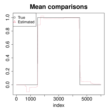
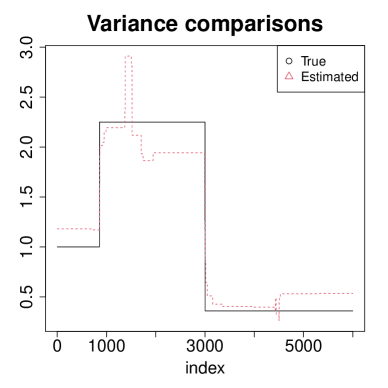
Figure 1: The left panel shows comparisons of the true and estimated means for Example 1 in the text. The right panel shows the corresponding variance comparisons.

Therefore, it is natural to estimate $v^{*}_{i}$ with

$$\hat{v}_{i}\,=\,\hat{\gamma}_{i}-(\hat{\theta}_{i})^{2},$$ (11)

where $\hat{\gamma}_{i}$ is an estimator of $\gamma_{i}^{*}:=\mathbb{E}(y_{i}^{2})$, and $\hat{\theta}$ is the fused lasso estimator defined in (2). As an estimator for $\gamma^{*}$, we propose

$$\hat{\gamma}\,:=\,\underset{\gamma\in\mathbb{R}^{n}}{\arg\min}\left\{\frac{1}{2}\sum_{i=1}^{n}(y_{i}^{2}-\gamma_{i})^{2}+\lambda^{\prime}\sum_{(i,j)\in E}|\gamma_{i}-\gamma_{j}|\right\}$$ (12)

for a tuning parameter $\lambda^{\prime}>0$.

Notice that $\hat{v}$ can be found with the same order of computational cost that it is required for finding $\hat{\theta}$. In practice, this can be done using the algorithm from Chambolle and Darbon (2009). As for the tuning parameter, we will give details about choosing $\lambda^{\prime}$ in practice in Section 4.2.

To illustrate the behavior of the estimator defined in (11)–(12), we now consider a simple numerical example. More comprehensive evluations will be given in Section 4.

Example 1.

We set $n=6000$ and generate data according to the model given by (1) with $\epsilon_{i}\overset{\text{ind}}{\sim}N(0,1)$ for $i=1,\ldots,n$, and $\theta^{*},v^{*}\in\mathbb{R}^{n}$ satisfying

$$\theta_{i}^{*}\,=\,\begin{cases}1&\text{if}\,\,\,n/4<i\leq 3n/4,\\ 0&\text{otherwise},\end{cases}$$

and

$$v_{i}^{*}\,=\,\begin{cases}1&\text{if}\,\,i\leq\lfloor n/7\rfloor,\\ 1.5^{2}&\text{if}\,\,\lfloor n/7\rfloor<i\leq n/2,\\ 0.6^{2}&\text{otherwise.}\end{cases}$$

Given the data $\{y_{i}\}_{i=1}^{n}$, we run the estimator defined in (11)–(12) with tuning parameter choices as discussed in Section 4.2. The results are displayed in Figure 1, where we see that the estimated means and variances are reasonably close to the corresponding true parameters.

3.1 A general result for fused lasso estimator

Before presenting our main result for the estimator $\hat{v}$ defined in (11)–(12), we provide a general upper bound for the fused lasso estimator that holds under very weak assumptions and generalizes existing work in Hütter and Rigollet (2016), Padilla et al. (2018) and Madrid Padilla et al. (2020b).

Theorem 2.

Consider data $\{o_{i}\}_{i=1}^{n}$ generated as $o_{i}=\beta_{i}^{*}+\varepsilon_{i}$ for some $\beta^{*}\in R^{n}$ and $\varepsilon_{1},\ldots,\varepsilon_{n}$ independent random variables satisfying satisfying $E(\varepsilon_{i})=0$ for $i=1,\ldots,n$, and $\max_{i=1,\ldots,n}E(\varepsilon_{i}^{4})=O(1)$. Let $\hat{\beta}$ be defined as

$$\hat{\beta}\,:=\,\underset{\beta\in\mathbb{R}^{n}}{\arg\min}\left\{\frac{1}{2}\sum_{i=1}^{n}(o_{i}-\beta_{i})^{2}+\lambda\sum_{(i,j)\in E}|\beta_{i}-\beta_{j}|\right\}.$$ (13)

The following results hold:

1. General graphs. For any connected graph $G$, if for a sequence $U_{n}$ it holds that

   $$\frac{n^{1/2}\,\underset{i=1,\ldots,n}{\max}(\mathbb{P}(|\varepsilon_{i}|>U_{n}))^{1/4}}{U_{n}\sqrt{\log(en)}\ }\,\rightarrow\,0,$$ (14)

   then

   $$\frac{\|\hat{\beta}-\beta^{*}\|^{2}}{n}\,=\,O_{\mathbb{P}}\left(\frac{U_{n}^{4/3}(\log n)^{1/3}\|\nabla_{G}\beta^{*}\|_{1}^{2/3}}{n^{2/3}}\,+\,\frac{U_{n}^{2}\log n}{n}\right),$$ (15)

   for a choice of $\lambda$ satisfying

   $$\lambda\,\asymp\,U_{n}^{4/3}(n\log n)^{1/3}\|\nabla_{G}\beta^{*}\|_{1}^{-1/3}.$$

2. Grid graphs. Let $G$ be the $d$-dimensional grid graph with $d>1$. Suppose that

   $$\frac{\underset{i=1,\ldots,n}{\max}n^{1/2}(\mathbb{P}(|\varepsilon_{i}|>U_{n}))^{1/4}}{U_{n}}\,\rightarrow\,0.$$ (16)

   Then there exists a choice of $\lambda$ satisfying

   $$\lambda\,\asymp\,U_{n}\phi_{n}\,+\,U_{n}\|\nabla_{G}\beta^{*}\|_{1}^{-1/2}$$

   such that

   $$\frac{\|\hat{\beta}-\beta^{*}\|^{2}}{n}\,=\,O_{\mathbb{P}}\left(\frac{U_{n}\phi_{n}\|\nabla_{G}\beta^{*}\|_{1}}{n}\,+\,\frac{U_{n}^{2}}{n}\right),$$ (17)

   where

   $$\phi_{n}\,:=\,\begin{cases}C(\log n)^{1/2}&\text{if}\,\,\,d=2,\\ C,\end{cases}$$ (18)

   for some constant $C>0$.

3. K-NN graphs. Suppose that in addition to the measurements $(y_{1},\ldots,y_{n})^{\top}$ we are also given covariates $\{x_{i}\}_{i=1}^{n}\subset\mathcal{X}$, where $x_{i}$ corresponds to $y_{i}$, and $\mathcal{X}$ is a metric space with metric $\mathrm{dist}(\cdot)$. Suppose that $\{(x_{i},y_{i})\}_{i=1}^{n}$ satisfy the assumptions from Madrid Padilla et al. (2020b), see Appendix C. In particular, $\mathcal{X}$ is homeomorphic to $[0,1]^{d}$. In addition, assume that $K\asymp\log^{1+2r}n$ for some $r>0$ in the construction of the $K$-NN graph $G$, and

   $$\frac{n^{1/2}\,\underset{i=1,\ldots,n}{\max}(\mathbb{P}(|\varepsilon_{i}|>U_{n}))^{1/4}}{U_{n}\sqrt{K}}\rightarrow 0.$$ (19)

   Then for an appropriate choice $\lambda$ it holds that

   $$\frac{\|\hat{\beta}-\beta^{*}\|^{2}}{n}\,=\,O_{\mathbb{P}}\left(\frac{U_{n}\mathrm{poly}(\log n)}{n^{1/d}}\right),$$ (20)

   where $\mathrm{poly}(\cdot)$ is a polynomial function.

Remark 3.

Let us now elaborate on (14), (16) and (19). Suppose, for instance, that $\varepsilon_{i}$ is sub-Exponential(a), for some constant $a>0$. Then the usual sub-Exponential tail inequality can be written as

$$\mathbb{P}(|\varepsilon_{i}|>t)\,\leq\,2\exp(-t/a),\,\,\,\,\text{for all }t>0,$$

see for instance Proposition 2.7.1 in Vershynin (2018). Hence, taking $U_{n}=4a\log n$ it follows that (14), (16) and (19) immediately hold. More generally, if

$$\mathbb{P}(|\varepsilon_{i}|>t)\,\leq\,c_{1}\exp(-t^{\alpha}/c_{2}),\,\,\,\text{for all }t>0,$$

for positive constants $c_{1},c_{2},$ and $\alpha$, then taking $U_{n}=4c_{2}(\log n)^{1/\alpha}$, we obtain that (14), (16) and (19) all hold.

Remark 4.

Remark 3 gives a family of examples where $U_{n}$ can be taken as a power function of $\log n$. More generally, if $U_{n}=O\{\mathrm{poly}(\log n)\}$, for a polynomial function $\mathrm{poly}$, then up to logarithmic factors, Theorem 2 gives the same rates as in several existing works on the fused lasso, but now we allow for more general error distributions than sub-Gaussian. Specifically:

1. For a connected graph $G$, (15) generalizes the upper bound in Theorem 3 in Padilla et al. (2018). Moreover, the same upper bound in (15) also holds if we replace the fused lasso estimator $\hat{\beta}$ (13) with the DFS fused lasso estimator from Padilla et al. (2018).

2. For a $d$-dimensional grid graph $G$, the rate in (17) matches that in Corollary 5 from Hütter and Rigollet (2016).

3. For nonparameteric regression, (20) gives the same minimax rate as Theorem 2 in Madrid Padilla et al. (2020b) for classes of piecewise functions.

Remark 5.

The proof of Theorem 2 actually follows from Theorem 4 in Section B. Theorem 4 essentially reduces the analysis of $\hat{\beta}$ to upper bounding

$$E\left(\underset{\beta\in R^{n}\,:\,\|\beta-\beta^{*}\|\leq\eta,\,\|\nabla_{G}\beta\|_{1}\leq 5\|\nabla_{G}\beta^{*}\|_{1}}{\sup}\sum_{i=1}^{n}\xi_{i}\varepsilon_{i}1_{\{|\varepsilon_{i}|\leq U_{n}\}}(\beta_{i}-\beta_{i}^{*})\right),$$ (21)

for some $\eta>0$, and where $\xi_{1},\ldots,\xi_{n}$ are independent Rademacher random variables independent of $\{\varepsilon_{i}\}_{i=1}^{n}$. In the proof of Theorem 4, the matrix $\nabla_{G}$ does not have to be the incidence matrix of a graph and, in fact, can be replaced with a general matrix $D$. For instance, $D$ can be the $(k+1)$th order difference matrix corresponding to trend filtering, see Tibshirani (2014). In that case, the quantity (21) can be upper bounded as in the proof of Theorem 4 to attain the usual rate $n^{-(2k+2)/(2k+3)}$, see Tibshirani (2014), ignoring factors involving powers of $\log n$ and $U_{n}$.

3.2 Fused lassor for variance estimation

We are now ready to state our main result regarding the estimator $\hat{v}$ defined in (11)–(12). Notably, our result shows that the estimator $\hat{v}$ enjoys similar properties as the original fused lasso in general graphs, $d$-dimensional grids, and $K$-NN graphs. The conclusion of our result follows from an application of Theorem 2 to $\hat{\theta}$ defined in (2) and $\hat{\gamma}$ defined in (12).

Theorem 3.

Consider data $\{y_{i}\}_{i=1}^{n}$ generated as in (1) and suppose that $\mathbb{E}(\epsilon_{i}^{8})<\infty$. Then the estimator $\hat{v}$ satisfies the following.

• General graphs. Let $G$ be any connected graph and assume that (14) holds with $\{\epsilon_{i}\}_{i=1}^{n}$ instead of $\{\varepsilon_{i}\}_{i=1}^{n}$. Then for choices of $\lambda$ and $\lambda^{\prime}$ satisfying

  $$\lambda\,\asymp\,U_{n}^{4/3}(n\log n)^{1/3}\|\nabla_{G}\theta^{*}\|_{1}^{-1/3}$$

  and

  $$\lambda^{\prime}\asymp[\sqrt{\|v^{*}\|_{1}}\|\theta^{*}\|_{\infty}U_{n}\,+\,\|v^{*}\|_{\infty}(1+U_{n}^{2})]^{4/3}(n\log n)^{1/3}\|\nabla_{G}\gamma^{*}\|_{1}^{-1/3}$$

  we have that

  $$\begin{array}[]{lll}\displaystyle\frac{1}{n}\|\hat{v}-v^{*}\|^{2}&\,=&\displaystyle O_{\mathbb{P}}\bigg{(}\frac{(\|\theta^{*}\|_{\infty}^{2}+1)(U_{n}^{\prime})^{4/3}(\log n)^{1/3}[\|\nabla_{G}v^{*}\|_{1}+\|\theta^{*}\|_{\infty}\|\nabla_{G}\theta^{*}\|_{1}]^{2/3}}{n^{2/3}}\,+\\ &&\,\,\,\,\,\,\,\,\displaystyle\frac{(\|\theta^{*}\|_{\infty}^{2}+1)(U_{n}^{\prime})^{2}\log n}{n}\bigg{)}\end{array}$$ (22)

  where

  $$U_{n}^{\prime}\,:=\,(2\sqrt{\|v^{*}\|_{\infty}}\|\theta^{*}\|_{\infty}+1)U_{n}+\,\|v^{*}\|_{\infty}U_{n}^{2}\,+\,\|v^{*}\|_{\infty}.$$ (23)

• Grid graphs. Let $G$ be the $d$-dimensional grid graph with $d>1$. Suppose that the sequence $\{\epsilon_{i}\}_{i=1}^{n}$ satisfies (16). Then there exists tuning parameter choices satisfying

  $$\lambda\,\asymp\,U_{n}\phi_{n}\,+\,U_{n}\|\nabla_{G}\theta^{*}\|_{1}^{-1/2}$$

  and

  $$\lambda^{\prime}\,\asymp\,U_{n}^{\prime}\phi_{n}\,+\,U_{n}^{\prime}\|\nabla_{G}\gamma^{*}\|_{1}^{-1/2}$$

  for which

  $$\frac{\|\hat{v}-v^{*}\|^{2}}{n}\,=\,O_{\mathbb{P}}\left(\frac{(\|\theta^{*}\|_{\infty}^{2}+1)U_{n}^{\prime}\phi_{n}\left[\|\nabla_{G}v^{*}\|_{1}+\|\theta^{*}\|_{\infty}\|\nabla_{G}\theta^{*}\|_{1}\right]}{n}\,+\,\frac{(\|\theta^{*}\|_{\infty}^{2}+1)(U_{n}^{\prime})^{2}}{n}\right),$$ (24)

  with $U^{\prime}_{n}$ as in (23) and $\phi_{n}$ as in (18).

• $K$-NN graphs. Suppose that in addition to the measurements $(y_{1},\ldots,y_{n})^{\top}$ we are also given covariates $\{x_{i}\}_{i=1}^{n}\subset\mathcal{X}$, where $x_{i}$ corresponds to $y_{i}$, and $\mathcal{X}$ is a metric space with metric $\mathrm{dist}(\cdot)$. Suppose that $\{(x_{i},y_{i})\}_{i=1}^{n}$ satisfy the assumptions from Madrid Padilla et al. (2020b) stated in Appendix D. In addition, assume that $K\asymp\log^{1+2r}n$ for some $r>0$ in the construction of the $K$-NN graph $G$, and (19) holds for $\{\epsilon_{i}\}_{i=1}^{n}$. Then for appropriate choices of $\lambda$ and $\lambda^{\prime}$, it holds that

  $$\frac{\|\hat{v}-v^{*}\|^{2}}{n}\,=\,O_{\mathbb{P}}\left(\frac{(\|\theta^{*}\|_{\infty}^{2}+1)U_{n}^{\prime}\phi_{n}\log^{1+2r}n}{n^{1/d}}\right),$$ (25)

  with $U^{\prime}_{n}$ as in (23).

Remark 6.

Consider the setting in which $\max\{\|\theta^{*}\|_{1},\|v^{*}\|_{\infty}\}=O(1)$, and $U_{n}=O(\mathrm{poly}(\log n))$, for $\mathrm{poly}$ a polynomial function. Then, ignoring logarithmic factors, Theorem 3 implies the following:

1. For a connected graph $G$, the estimator $\hat{v}$ satisfies

   $$\frac{\|\hat{v}-v^{*}\|^{2}}{n}\,=\,O_{\mathbb{P}}\left[\frac{\{\|\nabla_{G}\theta^{*}\|_{1}+\|\nabla_{G}v^{*}\|_{1}\}^{2/3}}{n^{2/3}}\right].$$

   Hence, for the chain graph and the canonical setting in which $\max\{\|\nabla_{G}\theta^{*}\|_{1},\|\nabla_{G}v^{*}\|_{1}\}=O(1)$, the estimator $\hat{v}$ attains the rate $n^{-2/3}$, which is minimax optimal in the class

   $$\{(v,\theta)\,:\,\max\{\|\nabla_{G}\theta^{*}\|_{1},\|\nabla_{G}v^{*}\|_{1}\}\,\leq\,C_{1},\,\max\{\|\theta^{*}\|_{\infty},\|v^{*}\|_{\infty}\}\,\leq\,C_{1}\}$$

   for some constants $C_{1},C_{2}>0$, see Theorem 4 in Shen et al. (2020).

2. If $d>1$, then for the $d$-dimensional grid graph, we obtain that

   $$\frac{\|\hat{v}-v^{*}\|^{2}}{n}\,=\,O_{\mathbb{P}}\left(n^{-1/d}\right),$$

   under the canonical scaling (see Sadhanala et al. (2016)) $\|\nabla_{G}\theta^{*}\|_{1},\|\nabla_{G}v^{*}\|_{1}\,\asymp\,n^{1-1/d}$. Hence, for estimating $v^{*}$, $\hat{v}$ attains the same rate that $\hat{\theta}$ acchieves but for estimating $\theta^{*}$, see Hütter and Rigollet (2016).

3. For the $K$-NN graph, $\hat{v}$ also attains the rate $n^{-1/d}$ for estimating piecewise Lipschitz functions, thereby maintaining the same adaptivity properties of $\hat{\theta}$ studied in Madrid Padilla et al. (2020b).

4 Experiments

4.1 Homoscedastic case

We start by exploring the performance of the estimator $\hat{v}$ defined in (8). We do this by generating data from the model in (1) with $\epsilon_{i}\overset{\text{ind}}{\sim}N(0,1)$ and $v_{i}^{*}=v_{0}^{*}$ for $i=1,\ldots,n$. We consider $2$-dimensional grid graphs $G$ with $n\in\{100^{2},200^{2},300^{2},400^{2}\}$, and we identify the nodes of $G$ with elements of the set $\{1,\ldots\,n^{1/2}\}\times\{1,\ldots,n^{1/2}\}$. Then we consider values of $v_{0}^{*}$ in $\{0.5,1,1.5,2\}$ and three different scenarios for the signal $\theta^{*}$. Next, we describe the choices of $\theta^{*}$ that we consider.

Scenario 1.

For $k,l\in\{1,\ldots,n^{1/2}\}$, we let

$$\theta^{*}_{k,l}\,=\,\begin{cases}1&\text{if}\,\,\,|k-n/2|<n/4,\,\,\text{and}\,\,|l-n/2|<n/8,\\ 0&\text{otherwise.}\end{cases}$$

Scenario 2.

We set

$$\theta^{*}_{k,l}\,=\,\begin{cases}1&\text{if}\,\,\,(k-n/4)^{2}+(l-n/4)^{2}<(n/5)^{2},\\ 0&\text{otherwise.}\end{cases}$$

Scenario 3.

In this scenario we set $\theta^{*}=0\in\mathbb{R}^{n^{1/2}\times n^{1/2}}$.

For each scenario and value of the model parameters, we generate 200 data sets, and for each data set, we compute the estimator $\hat{v}$ with a random DFS. We then compute the average of $|\hat{v}-v_{0}^{*}|$ across the 200 replicates and report the results in Tables 1–2. There, we can see that the estimator $\hat{v}$ performs reasonably well across all settings, with the performance improving as $n$ grows. Furthermore, as anticipated by Theorem 1, our estimator’s performance gets worse as $v_{0}^{*}$ grows.

Table 1: Performance evaluations of $\hat{v}$ for the different settings described in the text. We report $|\hat{v}-v_{0}^{*}|$ averaging over 200 Monte Carlo simulations.

Scenario	$v_{0}^{*}=0.5$				$v_{0}^{*}=1.0$
	$n=100^{2}$	$n=200^{2}$	$n=300^{2}$	$n=400^{2}$	$n=100^{2}$	$n=200^{2}$	$n=300^{2}$	$n=400^{2}$
1	0.07	0.05	0.05	0.04	0.17	0.12	0.08	0.07
2	0.08	0.06	0.05	0.04	0.16	0.10	0.10	0.08
3	0.07	0.05	0.05	0.04	0.17	0.12	0.08	0.08

Table 2: Performance evaluations of $\hat{v}$ for the different settings described in the text. We report $|\hat{v}-v_{0}^{*}|$ averaging over 200 Monte Carlo simulations.

Scenario	$v_{0}^{*}=1.5$				$v_{0}^{*}=2.0$
	$n=100^{2}$	$n=200^{2}$	$n=300^{2}$	$n=400^{2}$	$n=100^{2}$	$n=200^{2}$	$n=300^{2}$	$n=400^{2}$
1	0.24	0.18	0.14	0.13	0.31	0.23	0.18	0.16
2	0.24	0.17	0.14	0.14	0.27	0.20	0.19	0.18
3	0.25	0.16	0.14	0.13	0.30	0.23	0.17	0.16

4.2 Heteroscedastic case: Tuning parameters

We now proceed to evaluate the performance of the estimator $\hat{v}$ defined in (11)–(12). Before describing the different simulation settings, we now discuss how to choose the tuning parameters. Let $\hat{\theta}(\lambda)$ and $\hat{v}(\lambda^{\prime})$ the estimates based on choices $\lambda$ and $\lambda^{\prime}$. Notice that $\hat{v}(\lambda^{\prime})$ depends on $\lambda$ but we do not make this dependence explicit to avoid overloading the notation.

To choose $\lambda$, inspired by Tibshirani and Taylor (2012), we use a Bayesian information criterion given as

$$\widehat{\mathrm{BIC}}(\lambda)\,:=\,\|y-\hat{\theta}(\lambda)\|^{2}+2\widehat{\mathrm{df}}(\lambda)\log n$$

where $\widehat{\mathrm{df}}(\lambda)$ is the number of connected components induced by $\hat{\theta}(\lambda)$ in the graph $G$. Then we select the value of $\lambda$ that minimizes $\widehat{\mathrm{BIC}}(\lambda)$.

Once $\hat{\theta}(\lambda)$ has been computed, we proceed to select $\lambda^{\prime}$ for (12). We let $\hat{\gamma}(\lambda^{\prime})$ the solution to (12) and $\widetilde{\mathrm{df}}(\lambda^{\prime})$ be the number of connected components in $G$ induced by $\hat{\gamma}(\lambda^{\prime})$. Then we define

$$\widetilde{\mathrm{BIC}}(\lambda^{\prime})\,:=\,\sum_{i=1}^{n}(\min\{q,y_{i}^{2}\}-\hat{\gamma}(\lambda^{\prime})_{i})^{2}+2\widetilde{\mathrm{df}}(\lambda^{\prime})\log n$$ (26)

where $q$ is the $0.95$-quantile of the data $\{y_{i}^{2}\}_{i=1}^{n}$. We use $\min\{q,y_{i}^{2}\}$ in (26) to avoid the influence of outliers in the model selection step. With the above score in hand, we choose the value of $\lambda^{\prime}$ that minimizes $\widetilde{\mathrm{BIC}}(\lambda^{\prime})$. In all our experiments, we select $\lambda$ and $\lambda^{\prime}$ from the set $\{10^{1},10^{2},10^{3},10^{4},10^{5}\}$.

4.3 Heteroscedastic case: 2D Grid graphs

In our next experiment, we consider generative models where the true graph is a 2D grid graph of size $n^{1/2}\times n^{1/2}$. We generate data as in Section 4.1 with the difference that the variance is now not constant. The scenarios we consider are:

Scenario 4.

The signal $\theta^{*}$ is taken as in Scenario 3 from Section 4.1, and we let

$$v^{*}_{k,l}\,=\,\begin{cases}1.75&\text{if}\,\,\,|k-n/2|<n/3,\,\,\text{and}\,\,|l-n/2|<n/3,\\ 1&\text{otherwise,}\end{cases}$$

for $k,l\in\{1,\ldots,n^{1/2}\}$.

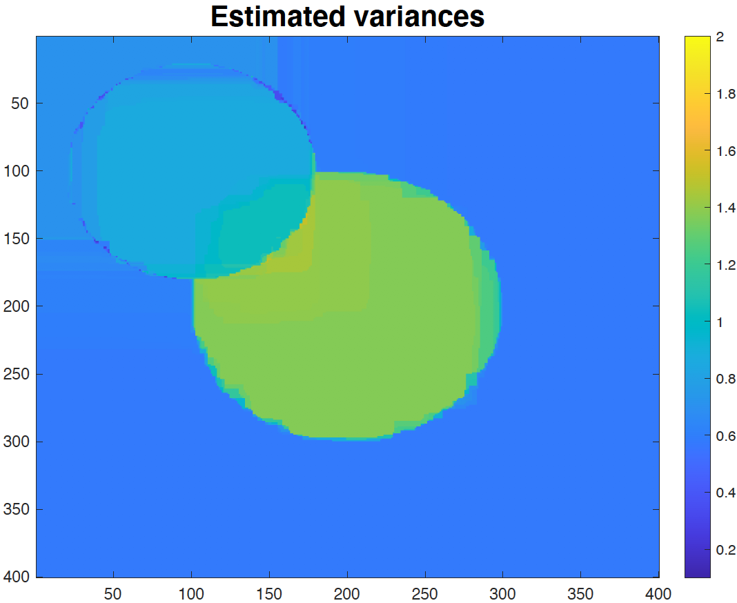
Figure 2: Each row corresponds to one scenario, with the top row corresponding to Scenario 4, the middle to Scenario 5, and the bottom to Scenario 6. The left column depicts the signals $\theta^{*}$, the middle column the signals $v^{*}$, and the right column the estimated $\hat{v}$.

Table 3: Performance evaluations of the estimator $\hat{v}$ defined in (11)–(12) for the different settings described in the text. We report the mean squared error averaging over 200 Monte Carlo simulations.

Scenario	$n=100^{2}$	$n=200^{2}$	$n=300^{2}$	$n=400^{2}$
4	0.14	0.05	0.03	0.02
5	0.05	0.05	0.03	0.02
6	0.12	0.07	0.04	0.03

Scenario 5.

We set

$$v^{*}_{k,l}\,=\,\begin{cases}1.5&\text{if}\,\,\,(k-n/2)^{2}+(l-n/2)^{2}<(n/4)^{2},\\ 0.5&\text{otherwise.}\end{cases}$$

for $k,l\in\{1,\ldots,n^{1/2}\}$ and take $\theta^{*}$ as in Scenario 2 in Section 4.1.

Scenario 6.

We let $\theta^{*}=0\in\mathbb{R}^{n^{1/2}\times n^{1/2}}$ and

$$v^{*}_{k,l}\,=\,\begin{cases}0.5&\text{if}\,\,\,(k-n/4)^{2}+(l-n/4)^{2}<(n/5)^{2},\\ 2&\text{if}\,\,\,(k-3n/4)^{2}+(l-3n/4)^{2}<(n/5)^{2},\\ 1&\text{otherwise.}\end{cases}$$

for $k,l\in\{1,\ldots,n^{1/2}\}$.

For each scenario and value of the tuning parameters, and for each data set, we compute the estimator $\hat{v}$ and choose the tuning parameters as in Section 4.2. We then report

$$\frac{1}{n}\|\hat{v}-v^{*}\|^{2}$$

averaging over 200 Monte Carlo simulations. The results in Table 3 show an excellent performance of our estimator, which becomes more evident as $n$ goes to $\infty$, which goes in line with our findings in Theorem 3.

Finally, Figure 2 provides visualizations of Scenarios 4–6 and the corresponding estimates $\hat{v}$ for one instance of $n=400^{2}$. There, we can see that $\hat{v}$ is a reasonable esimator of $v^{*}$, although $\hat{v}$ is afected by the bias induced by $\hat{\theta}$ which comes from Equation (11).

Figure 3: . For $n=120000$ and $d=2$, the top left panel shows a scatter plot of $\{(x_{i,1},x_{i,2},v_{i}^{*})\}_{i=1}^{n}$ for one instance of Scenarios 7 and 8. The top right panel displays the corresponding scatter plot of $\{(x_{i,1},x_{i,2},\hat{v}_{i})\}_{i=1}^{n}$ for Scenario 7. The bottom left panel is the scatter plot of $\{(x_{i,1},x_{i,2},f_{0}(x_{i}))\}_{i=1}^{n}$ for Scenario 8, and the bottom right panel shows the scatter plot of $\{(x_{i,1},x_{i,2},\hat{v}_{i})\}_{i=1}^{n}$ for Scenario 8.

4.4 Heteroscedastic case: $K$-NN graphs

In this experiment we consider a nonparametric regression setting. Specifically, we generate data from the model

$$\begin{array}[]{lll}y_{i}&=&f_{0}(x_{i})+\sqrt{v_{i}^{*}}\epsilon_{i},\\ v_{i}^{*}&=&g_{0}(x_{i})\\ \epsilon_{i}&\overset{\text{ind}}{\sim}&N(0,1),\\ x_{i}&\overset{\text{ind}}{\sim}&U[0,1]^{d},\end{array}$$

where $U[0,1]^{d}$ is the uniform distribution. In our simulations, we consider $d\in\{2,3\}$, $n\in\{1500,3000,6000,12000\}$, and difference choices of $f_{0}$ and $g_{0}$. The functions $f_{0}$ and $g_{0}$ are taken from the following scenarios:

Scenario 7.

In this scenario, we let $f_{0}(z)=0$ for all $z=(z_{1},\ldots,z_{d})^{\top}\in\mathbb{R}^{d}$ and

$$g_{0}(z)\,=\,\begin{cases}1.75&\text{if}\,\,\,z_{1}>0.5,\\ 0.25&\text{otherwise.}\end{cases}$$

Table 4: Performance evaluations of the estimator $\hat{v}$ defined in (11)–(12) for the different $K$-NN graph settings described in the text. We report the mean squared error averaging over 200 Monte Carlo simulations.

Scenario	$d=2$				$d=3$
	$n=1500$	$n=3000$	$n=6000$	$n=12000$	$n=1500$	$n=3000$	$n=6000$	$n=12000$
7	0.13	0.12	0.08	0.06	0.24	0.16	0.15	0.14
8	0.19	0.16	0.12	0.10	0.32	0.27	0.22	0.20

Scenario 8.

We let $g_{0}$ as in Scenario 7, and let

$$f_{0}(z)\,=\,\begin{cases}0&\text{if}\,\,\,z_{2}>0.5,\\ -1&\text{otherwise,}\end{cases}$$

for $z\in\mathbb{R}^{d}$

Based on the above scenarios, we generate 200 data sets and compute the mean squared error of our estimator in (11)–(12) averaging over all the repetitions. Our estimator is computed using the $K$-NN graph as defined in Appendix D with $K=5$. Table 4 seems to corroborate our findings in Theorem 3 as our method’s performance appears to improve with sample size but worsens when $d$ increases.

Finally, Figure 3 provides a visualization of the true signals and the estimated variances for one instance with $n=12000$ and $d=2$.

5 Ion channels data

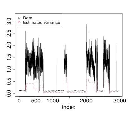
Figure 4: . Ion channels data and estimated variances

We now validate our method using a real data example. Specifically, we consider the Ion channels data used by Jula Vanegas et al. (2021). The original data was produced by the Steinem Lab (Institute of Organic and Biomolecular Chemistry, University of Gottingen). As explained by the Jula Vanegas et al. (2021), Ion channels are a class of proteins expressed by all cells that create pathways for ions to pass through the cell membrane. The data consist of a single ion channel of the bacterial porin PorB, a bacterium related to Neisseria gonorrhoeae.

Although the original data consists of 600000 time instances. We proceed as in Cappello et al. (2021) and construct a signal $y\in\mathbb{R}^{2048}$. The resulting data are plotted in Figure 4. There, we also see the estimated variances using our proposed method, which seems to capture the heteroscedastic nature of the data.

6 Conclusion

In this paper, we have studied the problem of estimating the variance in general graph denoising problems. We have proposed and analyzed estimators for both the homoscedastic and heteroscedastic cases. In studying the latter, we also proved generalizations of known bounds for the fused lasso estimator to models beyond sub-Gaussian errors.

Many research directions are left open in this work. One particular problem is to generalize our results to higher order versions of total variation for estimating the vector of variances. Constructing higher order versions of total variation is challenging in the case of estimating the mean in general graph-structured problems, and we expect it to be even more challenging for the variance case. Therefore, we leave this for future work.

Appendix A Proof of Theorem 1

Proof.

First, we observe that

$$\begin{array}[]{lll}|v_{0}^{*}-\hat{v}|&\leq&\displaystyle\bigg{|}v_{0}^{*}\,-\,\frac{v^{*}_{0}}{2(\lfloor n/2\rfloor-1)}\sum_{i=1}^{\lfloor n/2\rfloor-1}(\epsilon_{\sigma(2i)}-\epsilon_{\sigma(2i-1)})^{2}\bigg{|}\,+\\ &&\displaystyle\bigg{|}\frac{v_{0}^{*}}{2(\lfloor n/2\rfloor-1)}\sum_{i=1}^{\lfloor n/2\rfloor-1}(\epsilon_{\sigma(2i)}-\epsilon_{\sigma(2i-1)})^{2}\,-\\ &&\displaystyle\frac{1}{2(\lfloor n/2\rfloor-1)}\sum_{i=1}^{\lfloor n/2\rfloor-1}(\sqrt{v_{0}^{*}}\epsilon_{\sigma(2i)}-\sqrt{v_{0}^{*}}\epsilon_{\sigma(2i-1)}+\theta^{*}_{\sigma(2i)}-\theta^{*}_{\sigma(2i-1)})^{2}\bigg{|}.\end{array}$$

Next, using the identity $a^{2}-(a+b)^{2}=-b(2a+b)$ we obtain that

$$\begin{array}[]{lll}|v_{0}^{*}-\hat{v}|&\leq&\displaystyle\bigg{|}v_{0}^{*}\,-\,\frac{v^{*}_{0}}{2(\lfloor n/2\rfloor-1)}\sum_{i=1}^{\lfloor n/2\rfloor-1}(\epsilon_{\sigma(2i)}-\epsilon_{\sigma(2i-1)})^{2}\bigg{|}\,+\\ &&\displaystyle\frac{1}{2(\lfloor n/2\rfloor-1)}\sum_{i=1}^{\lfloor n/2\rfloor-1}|\theta^{*}_{\sigma(2i)}-\theta^{*}_{\sigma(2i-1)}|\,|2\sqrt{v^{*}_{0}}(\epsilon_{\sigma(2i)}-\epsilon_{\sigma(2i-1)})+(\theta^{*}_{\sigma(2i)}-\theta^{*}_{\sigma(2i-1)})|\\ &\leq&\displaystyle\bigg{|}v_{0}^{*}\,-\,\frac{v^{*}_{0}}{2(\lfloor n/2\rfloor-1)}\sum_{i=1}^{\lfloor n/2\rfloor-1}(\epsilon_{\sigma(2i)}-\epsilon_{\sigma(2i-1)})^{2}\bigg{|}\,+\\ &&\displaystyle\frac{(4\|\epsilon\|_{\infty}\sqrt{v_{0}^{*}}+2\|\theta^{*}\|_{\infty})}{2(\lfloor n/2\rfloor-1)}\sum_{i=1}^{\lfloor n/2\rfloor-1}|\theta^{*}_{\sigma(2i)}-\theta^{*}_{\sigma(2i-1)}|\\ &\leq&\displaystyle v_{0}^{*}\bigg{|}1\,-\,\frac{1}{2(\lfloor n/2\rfloor-1)}\sum_{i=1}^{\lfloor n/2\rfloor-1}(\epsilon_{\sigma(2i)}-\epsilon_{\sigma(2i-1)})^{2}\bigg{|}\,+\\ &&\displaystyle\frac{(4\|\epsilon\|_{\infty}\sqrt{v_{0}^{*}}+4\|\theta^{*}\|_{\infty}\|\nabla_{G}\theta^{*}\|_{1}}{2(\lfloor n/2\rfloor-1)}\\ \end{array}$$ (27)

where the last inequality follows from Lemma 1 in Padilla et al. (2018). Finally, notice that

$$\mathbb{E}\left(\frac{1}{2(\lfloor n/2\rfloor-1)}\sum_{i=1}^{\lfloor n/2\rfloor-1}(\epsilon_{\sigma(2i)}-\epsilon_{\sigma(2i-1)})^{2}\right)\,=\,1$$ (28)

and

$$\begin{array}[]{lll}\displaystyle\text{Var}\left(\frac{1}{2(\lfloor n/2\rfloor-1)}\sum_{i=1}^{\lfloor n/2\rfloor-1}(\epsilon_{\sigma(2i)}-\epsilon_{\sigma(2i-1)})^{2}\right)&=&\displaystyle\frac{1}{4(\lfloor n/2\rfloor-1)^{2}}\sum_{i=1}^{\lfloor n/2\rfloor-1}\text{Var}\left((\epsilon_{\sigma(2i)}-\epsilon_{\sigma(2i-1)})^{2}\right)\\ &\leq&\displaystyle\frac{1}{4(\lfloor n/2\rfloor-1)^{2}}\sum_{i=1}^{\lfloor n/2\rfloor-1}\mathbb{E}\left((\epsilon_{\sigma(2i)}-\epsilon_{\sigma(2i-1)})^{4}\right)\\ &\leq&\displaystyle\frac{1}{4(\lfloor n/2\rfloor-1)^{2}}\sum_{i=1}^{\lfloor n/2\rfloor-1}\mathbb{E}\left(8\epsilon_{\sigma(2i)}^{4}+8\epsilon_{\sigma(2i-1)}^{4}\right)\\ &\leq&\displaystyle\frac{4}{(\lfloor n/2\rfloor-1)}\underset{i=1,\ldots,n}{\sup}\,\mathbb{E}(\epsilon_{i}^{4})\\ \end{array}$$ (29)

where the second inequality follows from the inequality $(a+b)^{4}\leq 8a^{4}+8b^{4}$. Combining (27)–(29) with the Chebyshev’s inequality we conclude the proof. ∎

Appendix B A general upper bound

Theorem 4.

Consider data $\{o_{i}\}_{i=1}^{n}$ generated as $o_{i}=\beta_{i}^{*}+\varepsilon_{i}$ for some $\beta^{*}\in\mathbb{R}^{n}$ and $\varepsilon_{1},\ldots,\varepsilon_{n}$ independent random variables satisfying satisfying $\mathbb{E}(\varepsilon_{i})=0$ and

$$\underset{i=1,\ldots,n}{\max}\,\mathbb{E}(\varepsilon_{i}^{4})\,=\,O(1).$$

Let $\hat{\beta}$ be defined as

$$\hat{\beta}\,:=\,\underset{\beta\in\mathbb{R}^{n}}{\arg\min}\left\{\frac{1}{2}\sum_{i=1}^{n}(o_{i}-\beta_{i})^{2}+\lambda\sum_{(i,j)\in E}|\beta_{i}-\beta_{j}|\right\}.$$

Let $\eta>0$. Then any sequence $U_{n}>0$, we have that for any $\eta>0$ it holds that

$$\begin{array}[]{lll}\mathbb{P}(\|\hat{\beta}-\beta^{*}\|>\eta)&\leq&\displaystyle\frac{16n^{1/2}\underset{i=1,\ldots,n}{\max}(\mathbb{E}(\varepsilon_{i}^{4}))^{1/4}(\mathbb{P}(|\varepsilon_{i}|>U_{n}))^{1/4}}{\eta}\,+\\ &&\displaystyle\frac{16}{\eta^{2}}\,\mathbb{E}\left(\underset{\beta\in\mathbb{R}^{n}\,:\,\|\beta-\beta^{*}\|\leq\eta,\,\|\nabla_{G}\beta\|_{1}\leq 5\|\nabla_{G}\beta^{*}\|_{1}}{\sup}\sum_{i=1}^{n}\xi_{i}\varepsilon_{i}1_{\{|\varepsilon_{i}|\leq U_{n}\}}(\beta_{i}-\beta_{i}^{*})\right),\end{array}$$

where $\xi_{1},\ldots,\xi_{n}$ are independent Rademacher random variables independent of $\{\varepsilon_{i}\}_{i=1}^{n}$, provided that

$$\lambda\,=\,\frac{\eta^{2}}{4\|\nabla_{G}\beta^{*}\|_{1}}.$$ (30)

Proof.

First, notice that by convexity and the basic inequality we have that

$$\frac{1}{2}\sum_{i=1}^{n}(o_{i}-\beta_{i})^{2}+\lambda\|\nabla_{G}\beta\|_{1}\,\leq\,\frac{1}{2}\sum_{i=1}^{n}(o_{i}-\beta_{i}^{*})^{2}+\lambda\|\nabla_{G}\beta^{*}\|_{1}$$ (31)

for any $\beta\in\Lambda\,:=\,\{s\hat{\beta}+(1-s)\beta^{*}\,:\,s\in[0,1]\}$. Then

$$\|\nabla_{G}\beta\|_{1}\,\leq\,\|\nabla_{G}\beta\|_{1}\,+\,\frac{\|\beta-\beta^{*}\|^{2}}{2\lambda}\,\leq\,\frac{\varepsilon^{\top}(\beta-\beta^{*})}{\lambda}+\|\nabla_{G}\beta^{*}\|_{1}$$ (32)

for all $\beta\in\Lambda$. Ths implies

$$\begin{array}[]{lll}\displaystyle\|\nabla_{G}(\beta-\beta^{*})\|_{1}&\leq&\displaystyle\|\nabla_{G}\beta\|_{1}\,+\,\|\nabla_{G}\beta^{*}\|_{1}\\ &\leq&\displaystyle\frac{\varepsilon^{\top}(\beta-\beta^{*})}{\lambda}+2\|\nabla_{G}\beta^{*}\|_{1},\end{array}$$ (33)

for all $\beta\in\Lambda$.

Next, let $\beta\in\Lambda$ and suppose that $\|\beta-\beta^{*}\|^{2}\leq\eta^{2}$, and $\|\nabla_{G}\beta\|_{1}\geq 5\|\nabla_{G}\beta^{*}\|_{1}$. Then

$$\|\nabla_{G}(\beta-\beta^{*})\|_{1}\,\geq\,\|\nabla_{G}\beta\|_{1}-\|\nabla_{G}\beta^{*}\|_{1}\,\geq\,4\|\nabla_{G}\beta^{*}\|_{1}.$$

Hence, setting

$$s\,:=\,\frac{4\|\nabla_{G}\beta^{*}\|_{1}}{\|\nabla_{G}(\beta-\beta^{*})\|_{1}},$$

clearly $s\in[0,1]$, and we let

$$\beta^{\prime}:=s\beta+(1-s)\beta^{*}\in\Lambda.$$

Then

$$\|\beta^{\prime}-\beta^{*}\|^{2}\,\leq\,\|\beta-\beta^{*}\|^{2}\,\leq\,\eta^{2},$$

and

$$\begin{array}[]{lll}\|\nabla_{G}(\beta^{\prime}-\beta^{*})\|_{1}&=&s\|\nabla_{G}(\beta-\beta^{*})\|_{1}\\ &=&4\|\nabla_{G}\beta^{*}\|_{1}.\end{array}$$

Therefore, from (33),

$$4\|\nabla_{G}\beta^{*}\|_{1}\,=\,\|\nabla_{G}(\beta^{\prime}-\beta^{*})\|_{1}\,\leq\,\frac{\varepsilon^{\top}(\beta^{\prime}-\beta^{*})}{\lambda}+2\|\nabla_{G}\beta^{*}\|_{1}$$

which implies

$$2\|\nabla_{G}\beta^{*}\|_{1}\,\,\leq\,\frac{\varepsilon^{\top}(\beta^{\prime}-\beta^{*})}{\lambda}.$$

Hence, if we take

$$\lambda\,=\,\frac{\eta^{2}}{4\|\nabla_{G}\beta^{*}\|_{1}}$$

we obtain

$$\frac{\eta^{2}}{2}\,\leq\,\varepsilon^{\top}(\beta^{\prime}-\beta^{*}).$$

As a result, the events

$$\Omega_{1}\,:=\,\left\{\underset{\beta\in\Lambda\,:\,\|\beta-\beta^{*}\|\leq\eta}{\sup}\,\|\nabla_{G}\beta\|_{1}\,\geq\,5\|\nabla_{G}\beta^{*}\|_{1}\right\}$$

and

$$\Omega_{2}\,:=\,\left\{\underset{\beta\in\Lambda\,:\,\|\beta-\beta^{*}\|\leq\eta,\,\|\nabla_{G}(\beta-\beta^{*})\|_{1}\leq 4\|\nabla_{G}\beta^{*}\|_{1}}{\sup}\,\varepsilon^{\top}(\beta-\beta^{*})\,\geq\,\frac{\eta^{2}}{2}\right\}$$

satisfy that $\Omega_{1}\subset\Omega_{2}$. And so,

$$\mathbb{P}(\Omega_{1})\,\leq\,\mathbb{P}(\Omega_{2}).$$ (34)

Next, suppose that $\|\hat{\beta}-\beta^{*}\|>\eta$. Then there exists $\beta\in\Lambda$ such that $\|\beta-\beta^{*}\|=\eta$ and so (32) implies that

$$\frac{\eta^{2}}{2}\,\leq\,\varepsilon^{\top}(\beta-\beta^{*})\,+\,\lambda\|\nabla_{G}\beta^{*}\|_{1}\,-\,\lambda\|\nabla_{G}\beta\|_{1}.$$

Hence, given our choice of $\lambda$, we obtain that

$$\frac{\eta^{2}}{4}\,\leq\,\varepsilon^{\top}(\beta-\beta^{*}),$$

for some $\beta\in\Lambda$, provided that $\|\hat{\beta}-\beta^{*}\|>\eta$.

The above implies that

$$\begin{array}[]{lll}\mathbb{P}(\|\hat{\beta}-\beta^{*}\|>\eta)&\leq&\displaystyle\mathbb{P}(\{\|\hat{\beta}-\beta^{*}\|>\eta\}\cap\Omega_{1}^{c})\,+\,\mathbb{P}(\Omega_{1})\\ &\leq&\displaystyle\mathbb{P}(\{\|\hat{\beta}-\beta^{*}\|>\eta\}\cap\Omega_{1}^{c})\,+\,\mathbb{P}(\Omega_{2})\\ &\leq&\displaystyle\mathbb{P}\bigg{(}\underset{\beta\in\Lambda\,:\,\|\beta-\beta^{*}\|\leq\eta,\,\|\nabla_{G}\beta\|_{1}\leq 5\|\nabla_{G}\beta^{*}\|_{1}}{\sup}\varepsilon^{\top}(\beta-\beta^{*})\,\geq\,\frac{\eta^{2}}{4}\bigg{)}\,+\,\mathbb{P}(\Omega_{2})\\ &\leq&\displaystyle 2\mathbb{P}\bigg{(}\underset{\beta\in\Lambda\,:\,\|\beta-\beta^{*}\|\leq\eta,\,\|\nabla_{G}\beta\|_{1}\leq 5\|\nabla_{G}\beta^{*}\|_{1}}{\sup}\varepsilon^{\top}(\beta-\beta^{*})\,\geq\,\frac{\eta^{2}}{4}\bigg{)}\\ &\leq&\displaystyle\frac{8}{\eta^{2}}\,\mathbb{E}\left(\underset{\beta\in\Lambda\,:\,\|\beta-\beta^{*}\|\leq\eta,\,\|\nabla_{G}\beta\|_{1}\leq 5\|\nabla_{G}\beta^{*}\|_{1}}{\sup}\varepsilon^{\top}(\beta-\beta^{*})\right)\\ &=:&A_{1},\end{array}$$ (35)

where the second inequality follows from (34), and third from the discussion above, the fourth from the definition of $\Omega_{2}$, and the last inequality from Markov’s inequality. Next, notice that

$$\begin{array}[]{lll}A_{1}&\leq&\displaystyle\frac{8}{\eta^{2}}\,\mathbb{E}\left(\underset{\beta\in\Lambda\,:\,\|\beta-\beta^{*}\|\leq\eta,\,\|\nabla_{G}\beta\|_{1}\leq 5\|\nabla_{G}\beta^{*}\|_{1}}{\sup}\sum_{i=1}^{n}\varepsilon_{i}1_{\{|\varepsilon_{i}|\leq U_{n}\}}(\beta_{i}-\beta_{i}^{*})\right)\,+\\ &&\displaystyle\frac{8}{\eta^{2}}\,\mathbb{E}\left(\underset{\beta\in\Lambda\,:\,\|\beta-\beta^{*}\|\leq\eta,\,\|\nabla_{G}\beta\|_{1}\leq 5\|\nabla_{G}\beta^{*}\|_{1}}{\sup}\sum_{i=1}^{n}\varepsilon_{i}1_{\{|\varepsilon_{i}|>U_{n}\}}(\beta_{i}-\beta_{i}^{*})\right)\\ &\leq&\displaystyle\frac{8}{\eta^{2}}\,\mathbb{E}\left(\underset{\beta\in\Lambda\,:\,\|\beta-\beta^{*}\|\leq\eta,\,\|\nabla_{G}\beta\|_{1}\leq 5\|\nabla_{G}\beta^{*}\|_{1}}{\sup}\sum_{i=1}^{n}(\varepsilon_{i}1_{\{|\varepsilon_{i}|\leq U_{n}\}}-\mathbb{E}(\varepsilon_{i}1_{\{|\varepsilon_{i}|\leq U_{n}\}}))(\beta_{i}-\beta_{i}^{*})\right)\,+\\ &&\displaystyle\frac{8}{\eta^{2}}\,\underset{\beta\in\Lambda\,:\,\|\beta-\beta^{*}\|\leq\eta,\,\|\nabla_{G}\beta\|_{1}\leq 5\|\nabla_{G}\beta^{*}\|_{1}}{\sup}\sum_{i=1}^{n}\mathbb{E}(\varepsilon_{i}1_{\{|\varepsilon_{i}|\leq U_{n}\}})(\beta_{i}-\beta_{i}^{*})\,+\\ &&\displaystyle\frac{8}{\eta^{2}}\,\mathbb{E}\left(\underset{\beta\in\Lambda\,:\,\|\beta-\beta^{*}\|\leq\eta,\,\|\nabla_{G}\beta\|_{1}\leq 5\|\nabla_{G}\beta^{*}\|_{1}}{\sup}\sum_{i=1}^{n}\varepsilon_{i}1_{\{|\varepsilon_{i}|>U_{n}\}}(\beta_{i}-\beta_{i}^{*})\right)\\ &=:&A_{2}+A_{3}+A_{4},\end{array}$$

next we proceed to bound $A_{2}$, $A_{3}$ and $A_{4}$. To bound $A_{3}$, notice that since $\mathbb{E}(\varepsilon_{i})=0$ then

$$\begin{array}[]{lll}A_{3}&=&\displaystyle\frac{8}{\eta^{2}}\,\underset{\beta\in\Lambda\,:\,\|\beta-\beta^{*}\|\leq\eta,\,\|\nabla_{G}\beta\|_{1}\leq 5\|\nabla_{G}\beta^{*}\|_{1}}{\sup}\sum_{i=1}^{n}-\mathbb{E}(\varepsilon_{i}1_{\{|\varepsilon_{i}|>U_{n}\}})(\beta_{i}-\beta_{i}^{*}).\end{array}$$

Hence,

$$\begin{array}[]{lll}A_{3}&\leq&\displaystyle\frac{8n^{1/2}}{\eta}\,\underset{i=1,\ldots,n}{\max}|\mathbb{E}(\varepsilon_{i}1_{\{|\varepsilon_{i}|>U_{n}\}})|\\ &\leq&\displaystyle\frac{8n^{1/2}}{\eta}\,\underset{i=1,\ldots,n}{\max}\left(\mathbb{E}(\varepsilon_{i}^{2})\mathbb{E}(1_{\{|\varepsilon_{i}|>U_{n}\}})\right)^{1/2}\\ &=&\displaystyle\frac{8n^{1/2}}{\eta}\left(\underset{i=1,\ldots,n}{\max}\mathbb{E}(\varepsilon_{i}^{2})\mathbb{P}(|\varepsilon_{i}|>U_{n})\right)^{1/2},\end{array}$$ (36)

where the first and second inequalities follow from Cauchy–Schwarz inequality.

To bound $A_{4}$, we observe that

$$\begin{array}[]{lll}A_{4}&\leq&\displaystyle\frac{8}{\eta^{2}}\,\mathbb{E}\bigg{(}\underset{\beta\in\Lambda\,:\,\|\beta-\beta^{*}\|\leq\eta,\,\|\nabla_{G}\beta\|_{1}\leq 5\|\nabla_{G}\beta^{*}\|_{1}}{\sup}\bigg{(}\sum_{i=1}^{n}\varepsilon_{i}^{2}1_{\{|\varepsilon_{i}|>U_{n}\}}\bigg{)}^{1/2}\|\beta-\beta^{*}\|\bigg{)}\\ &\leq&\displaystyle\frac{8}{\eta}\,\mathbb{E}\bigg{(}\bigg{(}\sum_{i=1}^{n}\varepsilon_{i}^{2}1_{\{|\varepsilon_{i}|>U_{n}\}}\bigg{)}^{1/2}\bigg{)}\\ &\leq&\displaystyle\frac{8}{\eta}\,\bigg{(}\mathbb{E}\bigg{(}\sum_{i=1}^{n}\varepsilon_{i}^{2}1_{\{|\varepsilon_{i}|>U_{n}\}}\bigg{)}\bigg{)}^{1/2}\\ &\leq&\displaystyle\frac{8n^{1/2}}{\eta}\,\bigg{(}\underset{i=1,\ldots,n}{\max}\mathbb{E}\bigg{(}\varepsilon_{i}^{2}1_{\{|\varepsilon_{i}|>U_{n}\}}\bigg{)}\bigg{)}^{1/2}\\ &\leq&\displaystyle\frac{8n^{1/2}\max_{i=1,\ldots,n}(\mathbb{E}(\varepsilon_{i}^{4}))^{1/4}(\mathbb{P}(|\varepsilon_{i}|>U_{n}))^{1/4}}{\eta}.\end{array}$$ (37)

Let us now proceed to bound $A_{2}$. Let $\varepsilon_{1}^{\prime},\ldots,\varepsilon_{n}^{\prime}$ independent copies of $\varepsilon_{1},\ldots,\varepsilon_{n}$. Then for independent Rademacher random variables $\xi_{1},\ldots,\xi_{n}$, it holds that

$$\begin{array}[]{lll}A_{2}&\leq&\displaystyle\frac{8}{\eta^{2}}\,\mathbb{E}\left(\underset{\beta\in\Lambda\,:\,\|\beta-\beta^{*}\|\leq\eta,\,\|\nabla_{G}\beta\|_{1}\leq 5\|\nabla_{G}\beta^{*}\|_{1}}{\sup}\sum_{i=1}^{n}(\varepsilon_{i}1_{\{|\varepsilon_{i}|\leq U_{n}\}}-\varepsilon_{i}^{\prime}1_{\{|\varepsilon_{i}^{\prime}|\leq U_{n}\}})(\beta_{i}-\beta_{i}^{*})\right)\\ &=&\displaystyle\frac{8}{\eta^{2}}\,\mathbb{E}\left(\underset{\beta\in\Lambda\,:\,\|\beta-\beta^{*}\|\leq\eta,\,\|\nabla_{G}\beta\|_{1}\leq 5\|\nabla_{G}\beta^{*}\|_{1}}{\sup}\sum_{i=1}^{n}\xi_{i}(\varepsilon_{i}1_{\{|\varepsilon_{i}|\leq U_{n}\}}-\varepsilon_{i}^{\prime}1_{\{|\varepsilon_{i}^{\prime}|\leq U_{n}\}})(\beta_{i}-\beta_{i}^{*})\right)\\ &\leq&\displaystyle\frac{8}{\eta^{2}}\,\mathbb{E}\left(\underset{\beta\in\Lambda\,:\,\|\beta-\beta^{*}\|\leq\eta,\,\|\nabla_{G}\beta\|_{1}\leq 5\|\nabla_{G}\beta^{*}\|_{1}}{\sup}\sum_{i=1}^{n}\xi_{i}(\varepsilon_{i}1_{\{|\varepsilon_{i}|\leq U_{n}\}})(\beta_{i}-\beta_{i}^{*})\right)\,+\\ &&\displaystyle\frac{8}{\eta^{2}}\,\mathbb{E}\left(\underset{\beta\in\Lambda\,:\,\|\beta-\beta^{*}\|\leq\eta,\,\|\nabla_{G}\beta\|_{1}\leq 5\|\nabla_{G}\beta^{*}\|_{1}}{\sup}\sum_{i=1}^{n}-\xi_{i}(\varepsilon_{i}^{\prime}1_{\{|\varepsilon_{i}^{\prime}|\leq U_{n}\}})(\beta_{i}-\beta_{i}^{*})\right)\\ &=&\displaystyle\frac{16}{\eta^{2}}\,\mathbb{E}\left(\underset{\beta\in\Lambda\,:\,\|\beta-\beta^{*}\|\leq\eta,\,\|\nabla_{G}\beta\|_{1}\leq 5\|\nabla_{G}\beta^{*}\|_{1}}{\sup}\sum_{i=1}^{n}\xi_{i}(\varepsilon_{i}1_{\{|\varepsilon_{i}|\leq U_{n}\}})(\beta_{i}-\beta_{i}^{*})\right)\\ &\leq&\displaystyle\frac{16}{\eta^{2}}\,\mathbb{E}\left(\underset{\beta\in\mathbb{R}^{n}\,:\,\|\beta-\beta^{*}\|\leq\eta,\,\|\nabla_{G}\beta\|_{1}\leq 5\|\nabla_{G}\beta^{*}\|_{1}}{\sup}\sum_{i=1}^{n}\xi_{i}\varepsilon_{i}1_{\{|\varepsilon_{i}|\leq U_{n}\}}(\beta_{i}-\beta_{i}^{*})\right).\end{array}$$ (38)

The claim then follows.

∎

Appendix C Assumptions for $K$-NN graph for Theorem 2

We start by explicitly defining the construction of the $K$- NN graph. Specifically, $(i,j)\in E$ if and only if $x_{j}$ is among the $K$-nearest neighbors (with respect to the metric $\mathrm{dist}(\cdot$) of $x_{i}$, or vice versa.

We now state the assumptions from Madrid Padilla et al. (2020b) needed for Theorem 2. Throughout $(\mathcal{X},\mathrm{dist})$ is a metric space with Borel sets $\mathcal{B}(\mathcal{X})$.

Assumption 2.

The covariates $\{x_{i}\}$ are independent draws from a density $p$, with respect to the measurable space $(\mathcal{X},\mathcal{B}(\mathcal{X}),\mu)$, with support $\mathcal{X}$. Furthermore, the density $p$ satisfies $0<p_{\min}<p(x)<p_{\max}$ for all $x\in\mathcal{X}$, where $p_{\min}$ and $p_{\max}$ are constants.

Assumption 3.

The base measure satisfies

$$c_{1}r^{d}\,\leq\,\mu\left(\{q\in\mathcal{X}\,:\,\mathrm{dist}(q,x)\leq r\}\right)\,\leq\,c_{2}r^{d}$$

for all $x\in\mathcal{X}$, and all $0<r<r_{0}$, where $c_{1}$, $c_{2}$ and $r_{0}$ are all positive constants, and $d\in\mathbb{N}\backslash\{0\}$ is the intrinsic dimension of $\mathcal{X}$.

Assumption 4.

There exists a homeomorphism (a continuous bijection with a continuous inverse) $h\,:\,\mathcal{X}\rightarrow[0,1]^{d}$ such that

$$L_{\min}\mathrm{dist}(x,x^{\prime})\,\leq\,\|h(x)-h(x^{\prime})\|\,\leq\,L_{\max}\mathrm{dist}(x,x^{\prime}),\,\,\,\forall x,x^{\prime}\in\mathcal{X},$$

for some positive constants $L_{\min}$ and $L_{\max}$.

For a set $S\subset[0,1]^{d}$, we let

$$B_{t}(S)\,:=\,\{q\in[0,1]^{d}\,:\,\|q-q^{\prime}\|\leq t\,\,\text{for some }\,\,q^{\prime}\in S\}.$$

With this notation, we state our next assumption.

Assumption 5.

[Piecewise Lipschitz]. The parameter $\beta^{*}$ satisfies that $\beta_{i}^{*}=f_{0}(x_{i})$ for $i=1,\ldots,n$ for some function $f_{0}$, where the following holds for the function $f_{0}$.

1. $f_{0}$ is bounded.

2. Let $\partial[0,1]^{d}$ be the boundary of $[0,1]^{d}$, and let $\Omega_{t}=[0,1]^{d}\backslash B_{t}(\partial[0,1]^{d})$. We assume that there exists a set $\mathcal{S}$ such that:

   1. The set $\mathcal{S}$ has Lebesgue measure zero.

   2. For some constants $C_{\mathcal{S}},t_{0}>0$, we have that

      $$\mu\left(h^{-1}\left(B_{t}(\mathcal{S})\cup([0,1]^{d}\backslash\Omega_{t})\right)\right)\,\leq\,C_{\mathcal{S}}t$$

      for all $0<t<t_{0}$.

   3. There exists a positive constant $L_{0}$ such that if $z$ and $z^{\prime}$ belong to the same connected component of $\Omega_{t}\backslash B_{t}(\mathcal{S})$ then

      $$|f_{0}\circ h^{-1}(z)-f_{0}\circ h^{-1}(z^{\prime})|\,\leq\,L_{0}\|z-z^{\prime}\|.$$

Appendix D Assumptions for $K$-NN graph for Theorem 3

We assume that the covariates $\{x_{i}\}_{i=1}^{n}$ satisfy Assumptions 2–4. In addition, we assume that Assumption 5 holds replacing $\beta^{*}$ with both $v^{*}$ and $\theta^{*}$.

Appendix E Proof of Theorem 2

Proof.

Proof of (15): First, let $G^{\prime}$ be a chain graph corresponding to a DFS ordering in $G$. Based of Theorem 4, we first need to bound

$$B_{1}:=\displaystyle\frac{16}{\eta^{2}}\,\mathbb{E}\left(\underset{\beta\in\mathbb{R}^{n}\,:\,\|\beta-\beta^{*}\|\leq\eta,\,\|\nabla_{G}\beta\|_{1}\leq 5\|\nabla_{G}\beta^{*}\|_{1}}{\sup}\sum_{i=1}^{n}\xi_{i}\varepsilon_{i}1_{\{|\varepsilon_{i}|\leq U_{n}\}}(\beta_{i}-\beta_{i}^{*})\right).$$ (39)

To bound this, we recall Lemma 1 in Padilla et al. (2018) which implies that $\|\nabla_{G^{\prime}}\beta\|_{1}\leq 2\|\nabla_{G}\beta\|_{1}$ for all $\beta\in\mathbb{R}^{n}$. Hence,

$$\begin{array}[]{lll}B_{1}&\leq&\displaystyle\frac{16}{\eta^{2}}\,\mathbb{E}\left(\underset{\beta\in\mathbb{R}^{n}\,:\,\|\beta-\beta^{*}\|\leq\eta,\,\|\nabla_{G^{\prime}}\beta\|_{1}\leq 10\|\nabla_{G}\beta^{*}\|_{1}}{\sup}\sum_{i=1}^{n}\xi_{i}\varepsilon_{i}1_{\{|\varepsilon_{i}|\leq CU_{n}\}}(\beta_{i}-\beta_{i}^{*})\right)\\ &\leq&\displaystyle\frac{16}{\eta^{2}}\mathbb{E}\left(\mathbb{E}\left(\underset{\beta\in\mathbb{R}^{n}\,:\,\|\beta-\beta^{*}\|\leq\eta,\,\|\nabla_{G^{\prime}}\beta\|_{1}\leq 10\|\nabla_{G}\beta^{*}\|_{1}}{\sup}\sum_{i=1}^{n}\xi_{i}\varepsilon_{i}1_{\{|\varepsilon_{i}|\leq U_{n}\}}(\beta_{i}-\beta_{i}^{*})\,\bigg{|}\varepsilon\right)\right)\\ &=&\displaystyle\frac{16U_{n}}{\eta^{2}}\mathbb{E}\left(\mathbb{E}\left(\underset{\beta\in\mathbb{R}^{n}\,:\,\|\beta-\beta^{*}\|\leq\eta,\,\|\nabla_{G^{\prime}}\beta\|_{1}\leq 10\|\nabla_{G}\beta^{*}\|_{1}}{\sup}\sum_{i=1}^{n}\xi_{i}\frac{\varepsilon_{i}}{U_{n}}1_{\{|\varepsilon_{i}|\leq U_{n}\}}(\beta_{i}-\beta_{i}^{*})\,\bigg{|}\varepsilon\right)\right).\end{array}$$ (40)

Then

$$\begin{array}[]{l}\displaystyle\mathbb{E}\bigg{(}\underset{\beta\in\mathbb{R}^{n}\,:\,\|\beta-\beta^{*}\|\leq\eta,\,\|\nabla_{G^{\prime}}\beta\|_{1}\leq 10\|\nabla_{G}\beta^{*}\|_{1}}{\sup}\sum_{i=1}^{n}\xi_{i}\frac{\varepsilon_{i}}{U_{n}}1_{\{|\varepsilon_{i}|\leq U_{n}\}}(\beta_{i}-\beta_{i}^{*})\,\bigg{|}\varepsilon\bigg{)}\\ \displaystyle\leq\displaystyle\mathbb{E}\bigg{(}\underset{\beta\in\mathbb{R}^{n}\,:\,\|\beta-\beta^{*}\|\leq\eta,\,\|\nabla_{G^{\prime}}(\beta-\beta^{*})\|_{1}\leq 11\|\nabla_{G}\beta^{*}\|_{1}}{\sup}\sum_{i=1}^{n}\xi_{i}\frac{\varepsilon_{i}}{U_{n}}1_{\{|\varepsilon_{i}|\leq U_{n}\}}(\beta_{i}-\beta_{i}^{*})\,\bigg{|}\varepsilon\bigg{)}\\ \displaystyle\leq\displaystyle\mathbb{E}\bigg{(}\underset{\beta\in\mathbb{R}^{n}\,:\,\|\beta\|\leq\eta,\,\|\nabla_{G^{\prime}}\beta\|_{1}\leq 11\|\nabla_{G}\beta^{*}\|_{1}}{\sup}\sum_{i=1}^{n}\xi_{i}\frac{\varepsilon_{i}}{U_{n}}1_{\{|\varepsilon_{i}|\leq U_{n}\}}\beta_{i}\,\bigg{|}\varepsilon\bigg{)}\\ \displaystyle\leq\displaystyle\mathbb{E}\bigg{(}\underset{\beta\in\mathbb{R}^{n}\,:\,\|\beta\|\leq\eta,\,\|\nabla_{G^{\prime}}\beta\|_{1}\leq 11\|\nabla_{G}\beta^{*}\|_{1}}{\sup}\sum_{i=1}^{n}\xi_{i}\beta_{i}\,\bigg{|}\varepsilon\bigg{)}\\ \end{array}$$

where the last inequality follows from Theorem 4.12 in Ledoux and Talagrand (1991). As a result, letting $\tilde{\xi}_{i}\overset{\text{ind}}{\sim}N(0,1)$ for $i=1,\ldots,n$, we obtain that

$$\begin{array}[]{l}\displaystyle\mathbb{E}\bigg{(}\underset{\beta\in\Lambda\,:\,\|\beta-\beta^{*}\|\leq\eta,\,\|\nabla_{G^{\prime}}\beta\|_{1}\leq 10\|\nabla_{G}\beta^{*}\|_{1}}{\sup}\sum_{i=1}^{n}\xi_{i}\frac{\varepsilon_{i}}{U_{n}}1_{\{|\varepsilon_{i}|\leq U_{n}\}}(\beta_{i}-\beta_{i}^{*})\,\bigg{|}\varepsilon\bigg{)}\\ \displaystyle\leq\displaystyle\mathbb{E}\bigg{(}\underset{\beta\in\mathbb{R}^{n}\,:\,\|\beta\|\leq\eta,\,\|\nabla_{G^{\prime}}\beta\|_{1}\leq 11\|\nabla_{G}\beta^{*}\|_{1}}{\sup}\sum_{i=1}^{n}\xi_{i}\beta_{i}\,\bigg{)}\\ \displaystyle\leq\displaystyle\left(\frac{\pi}{2}\right)^{1/2}\mathbb{E}\bigg{(}\underset{\beta\in\mathbb{R}^{n}\,:\,\|\beta\|\leq\eta,\,\|\nabla_{G^{\prime}}\beta\|_{1}\leq 11\|\nabla_{G}\beta^{*}\|_{1}}{\sup}\sum_{i=1}^{n}\tilde{\xi}_{i}\beta_{i}\,\bigg{)}\\ \displaystyle\leq\,C_{1}\bigg{[}\eta\bigg{(}\frac{11\|\nabla_{G}\beta^{*}\|_{1}n^{1/2}}{\eta}\bigg{)}^{1/2}\,+\,\eta\sqrt{\log(en)}\bigg{]}\end{array}$$

where the second inequality follows fromt a well known fact bounding Rademacher Width by Gaussian Width; e.g see Page 132 in Wainwright (2019), and the last by Lemma B.1 from Guntuboyina et al. (2020). This implies that

$$B_{1}\,\leq\,\frac{16U_{n}}{\eta^{2}}\,C_{1}\bigg{[}\eta\bigg{(}\frac{11\|\nabla_{G}\beta^{*}\|_{1}n^{1/2}}{\eta}\bigg{)}^{1/2}\,+\,\eta\sqrt{\log(en)}\bigg{]}.$$

Therefore, given $a\in(0,1)$, we let

$$\eta\,:=\,\frac{4}{a}\left[16^{2/3}n^{1/6}(\log n)^{1/6}(11)^{1/3}\|\nabla_{G}\beta^{*}\|_{1}^{1/3}U_{n}^{2/3}(C_{1})^{2/3}\,+\,16C_{1}U_{n}\sqrt{\log(en)}\right]$$

and $\lambda$ as in (30). Hence,

$$\begin{array}[]{lll}B_{1}&\leq&\displaystyle\frac{16C_{1}U_{n}(11\|\nabla_{G}\beta^{*}\|_{1})^{1/2}n^{1/4}}{\eta^{3/2}}\,+\,\frac{16C_{1}U_{n}\sqrt{\log(en)}}{\eta}\\ &\leq&\displaystyle\frac{a^{3/2}}{4^{3/2}}\frac{16C_{1}U_{n}(11\|\nabla_{G}\beta^{*}\|_{1})^{1/2}n^{1/4}}{\left[16^{2/3}n^{1/6}(\log n)^{1/6}(11)^{1/3}\|\nabla_{G}\beta^{*}\|_{1}^{1/3}U_{n}^{2/3}(C_{1})^{2/3}\right]^{3/2}}\,+\,\frac{a}{4}\\ &\leq&\displaystyle\frac{a}{2}.\end{array}$$ (41)

Furthermore, by Theorem 4, we must bound

$$B_{2}\,:=\,\displaystyle\frac{16n^{1/2}\,\underset{i=1,\ldots,n}{\max}(\mathbb{E}(\varepsilon_{i}^{4}))^{1/4}(\mathbb{P}(|\varepsilon_{i}|>U_{n}))^{1/4}}{\eta}.$$ (42)

However, given our definition of $\eta$, we obtain that

$$\begin{array}[]{lll}B_{2}&\leq&\displaystyle\frac{a}{4}\,\frac{16n^{1/2}\,\underset{i=1,\ldots,n}{\max}(\mathbb{E}(\varepsilon_{i}^{4}))^{1/4}(\mathbb{P}(|\varepsilon_{i}|>U_{n}))^{1/4}}{\left[16^{2/3}n^{1/6}(\log n)^{1/6}(11)^{1/3}\|\nabla_{G}\beta^{*}\|_{1}^{1/3}U_{n}^{2/3}(C_{1})^{2/3}\,+\,16C_{1}U_{n}\sqrt{\log(en)}\right]}\\ &\leq&\displaystyle\frac{a}{4}\end{array}$$

where the last inequality follows from (14). The conclusion of the Theorem follows from Theorem 4.

Proof of rate (17): As before, we first bound $B_{1}$ as defined in (39). Towards that end, let $\nabla_{G}^{+}$ the pseudo inverse of $\nabla_{G}$, and $\Pi$ the orthogonal projection onto the span of $(1,\ldots,1)^{\top}\in\mathbb{R}^{n}$. Then notice that

$$\begin{array}[]{lll}B_{1}&\leq&\displaystyle\frac{16U_{n}}{\eta^{2}}\,\mathbb{E}\left(\underset{\delta\in\mathbb{R}^{n}\,:\,\|\delta\|\leq\eta,\,\|\nabla_{G}\delta\|_{1}\leq 6\|\nabla_{G}\beta^{*}\|_{1}}{\sup}\sum_{i=1}^{n}\frac{\xi_{i}\varepsilon_{i}1_{\{|\varepsilon_{i}|\leq U_{n}\}}}{U_{n}}\delta_{i}\right)\\ &\leq&\displaystyle\frac{16U_{n}}{\eta^{2}}\,\mathbb{E}\left(\underset{\delta\in\mathbb{R}^{n}\,:\,\|\delta\|\leq\eta,\,\|\nabla_{G}\delta\|_{1}\leq 6\|\nabla_{G}\beta^{*}\|_{1}}{\sup}\tilde{\varepsilon}^{\top}\nabla_{G}^{+}\nabla_{G}\delta\right)\,+\\ &&\displaystyle\frac{16U_{n}}{\eta^{2}}\,\mathbb{E}\left(\underset{\delta\in\mathbb{R}^{n}\,:\,\|\delta\|\leq\eta,\,\|\nabla_{G}\delta\|_{1}\leq 6\|\nabla_{G}\beta^{*}\|_{1}}{\sup}\tilde{\varepsilon}^{\top}\Pi\delta\right),\\ \end{array}$$

where $\tilde{\varepsilon}_{i}=\xi_{i}\varepsilon_{i}1_{\{|\varepsilon_{i}|\leq U_{n}\}}/U_{n}$ for $i=1,\ldots,n$. Next, we observe that by Hölder’s inequality and Cauchy–Schwarz inequality, it holds that ,

$$\begin{array}[]{lll}B_{1}&\leq&\displaystyle\frac{96U_{n}\|\nabla_{G}\beta^{*}\|_{1}}{\eta^{2}}\mathbb{E}\left(\|\big{(}\nabla_{G}^{+}\big{)}^{\top}\tilde{\varepsilon}\|_{\infty}\right)\,+\,\frac{16U_{n}}{\eta^{2}}\,\mathbb{E}\left(\underset{\delta\in\mathbb{R}^{n}\,:\,\|\delta\|\leq\eta,\,\|\nabla_{G}\delta\|_{1}\leq 6\|\nabla_{G}\beta^{*}\|_{1}}{\sup}\tilde{\varepsilon}^{\top}\Pi\delta\right)\\ &=&\displaystyle\frac{96U_{n}\|\nabla_{G}\beta^{*}\|_{1}}{\eta^{2}}\mathbb{E}\left(\|\big{(}\nabla_{G}^{+}\big{)}^{\top}\tilde{\varepsilon}\|_{\infty}\right)\,+\,\frac{16U_{n}}{\eta^{2}}\underset{\delta\,:\,\|\delta\|\leq\eta}{\sup}\bigg{(}\frac{1}{\sqrt{n}}\sum_{i=1}^{n}\delta_{i}\bigg{)}\mathbb{E}\bigg{(}\bigg{|}\frac{1}{\sqrt{n}}\sum_{i=1}^{n}\tilde{\varepsilon}_{i}\bigg{|}\bigg{)}\\ &\leq&\displaystyle\frac{96U_{n}\|\nabla_{G}\beta^{*}\|_{1}}{\eta^{2}}\mathbb{E}\left(\|\big{(}\nabla_{G}^{+}\big{)}^{\top}\tilde{\varepsilon}\|_{\infty}\right)\,+\,\frac{16U_{n}}{\eta}\mathbb{E}\bigg{(}\bigg{|}\frac{1}{\sqrt{n}}\sum_{i=1}^{n}\tilde{\varepsilon}_{i}\bigg{|}\bigg{)}\\ &\leq&\displaystyle\frac{96U_{n}\|\nabla_{G}\beta^{*}\|_{1}}{\eta^{2}}\mathbb{E}\left(\|\big{(}\nabla_{G}^{+}\big{)}^{\top}\tilde{\varepsilon}\|_{\infty}\right)\,+\,\frac{16U_{n}}{\eta}\\ &\leq&\displaystyle\frac{96U_{n}\|\nabla_{G}\beta^{*}\|_{1}}{\eta^{2}}\underset{j}{\max}\|(\nabla_{G}^{+})_{,j}\|\,+\,\frac{16U_{n}}{\eta}\\ \end{array}$$

where the third and last inequalities follow from the Sub-Gaussian maximal inequality. Next, by Propositions 4 and 6 from Hütter and Rigollet (2016), we obtain that

$$\underset{j}{\max}\|(\nabla_{G}^{+})_{,j}\|\,\leq\,\phi_{n}\,:=\,\begin{cases}C(\log n)^{1/2}&\text{if}\,\,\,d=2,\\ C,\end{cases}$$ (43)

for some constant $C>0$. Therefore,

$$B_{1}\,\leq\,\frac{96U_{n}\|\nabla_{G}\beta^{*}\|_{1}\phi_{n}}{\eta^{2}}\,+\,\frac{16U_{n}}{\eta}.\\$$

Hence, for a given $a\in(0,1)$, we let

$$\eta\,:=\,\frac{2}{a^{1/2}}(96U_{n}\|\nabla_{G}\beta^{*}\|_{1}\phi_{n})^{1/2}+\frac{4}{a}\cdot 16U_{n}$$

and $\lambda$ as in (30).

Therefore,

$$B_{1}\,\leq\,\frac{a^{2}}{4}+\frac{a}{4}\,\leq\,\frac{a}{2}.$$

Moreover, from (42), we have that

$$\begin{array}[]{lll}B_{2}&=&\displaystyle\frac{16n^{1/2}\,\underset{i=1,\ldots,n}{\max}(\mathbb{E}(\varepsilon_{i}^{4}))^{1/4}(\mathbb{P}(|\varepsilon_{i}|>U_{n}))^{1/4}}{\eta}\\ &\leq&\displaystyle\frac{a}{4}\frac{n^{1/2}\,\underset{i=1,\ldots,n}{\max}(\mathbb{E}(\varepsilon_{i}^{4}))^{1/4}(\mathbb{P}(|\varepsilon_{i}|>U_{n}))^{1/4}}{U_{n}}\\ &\leq&\displaystyle\frac{a}{4}.\end{array}$$

Therefore,

$$\mathbb{P}(\|\hat{\beta}-\beta^{*}\|>\eta)\,\leq\,\frac{3a}{4}.$$

This proves (17).

Proof of (20): First, by Madrid Padilla et al. (2020a), there exists $N$ satisfying $N\asymp(n/K)^{1/d}$ and functions $I\,:\,\mathbb{R}^{n}\,\rightarrow\mathbb{R}^{n}$, and $\tilde{I}\,:\,\mathbb{R}^{n}\,\rightarrow\mathbb{R}^{N^{d}}$ satisfying the properties below.

• [Lemma 8 in Madrid Padilla et al. (2020b)]. Let $\mathcal{E}_{1}$ be the event such that

  $$|e^{\top}(\beta-I(\beta))|\,\leq\,2\|e\|_{\infty}\|\nabla_{G}\beta\|_{1},\,\,\,\,\,\forall\beta,e\in\mathbb{R}^{n},$$ (44)

  and there exists a $d$-dimensional lattice $G^{\prime}$ with $N^{d}$ nodes such that

  $$\|\nabla_{G^{\prime}}\tilde{I}(\beta)\|_{1}\,\leq\,\|\nabla_{G}\beta\|_{1},\,\,\,\,\,\forall\beta\in\mathbb{R}^{n}.$$ (45)

  Then $\mathbb{P}(\mathcal{E}_{1})\rightarrow 1$.

• [Lemmas 7, 8 and 10 in Madrid Padilla et al. (2020b)]. Le $e$ be any vector of mean zero independent subg-Gaussian($\sigma^{2}$), then there exists $\tilde{e}$ a vector of mean zero independent sub-Gaussian($\sigma^{2}$) random variables and a constant $C>0$(not depending on $e$) such that the event $\mathcal{E}_{2}$ given as

  $$\begin{array}[]{lll}\mathcal{E}_{2}&\,:=&\bigg{\{}e^{\top}\{I(\beta)-I(\beta^{*})\}\,\leq\,CK^{1/2}\bigg{\{}\|\Pi\tilde{e}\|_{2}\|\beta-\beta^{*}\|\,+\,\|(\nabla_{G^{\prime}})^{+}\tilde{e}\|_{\infty}(\|\nabla_{G}\beta^{*}\|_{1}+\|\nabla_{G}\beta\|_{1})\bigg{\}},\\ &&\,\,\,\,\,\,\,\,\forall\beta\in R^{n},\,\,\,\,\forall e\,\,\text{vector of mean zero independent sub-Gaussian}(\sigma^{2})\bigg{\}}\end{array}$$ (46)

  satisfies $\mathbb{P}(\mathcal{E}_{2})\rightarrow 1$.

• Theorem 2 in Madrid Padilla et al. (2020b)]. It holds that for some constant $C_{2}>0$ the event

  $$\mathcal{E}_{3}\,:=\,\left\{\|\nabla_{G}\beta^{*}\|_{1}\,\leq\,C_{2}\text{poly}(\log n)n^{1-1/d}\right\}$$

  satisfies $\mathbb{P}(\mathcal{E}_{3})\rightarrow 1$, where $\text{poly}(\cdot)$ is a polynomial function.

Let $\mathcal{E}_{4}=\mathcal{E}_{1}\cap\mathcal{E}_{2}\cap\mathcal{E}_{3}$ Notice that as in Theorem 4, with the choice

$$\lambda\,=\,\frac{\eta^{2}}{4\|\nabla_{G}\beta^{*}\|_{1}},$$

we have that

$$\begin{array}[]{lll}\mathbb{P}(\|\hat{\beta}-\beta^{*}\|>\eta|\mathcal{E}_{4})&\leq&\displaystyle\frac{16n^{1/2}\,\underset{i=1,\ldots,n}{\max}(\mathbb{E}(\varepsilon_{i}^{4}))^{1/4}(\mathbb{P}(|\varepsilon_{i}|>U_{n}))^{1/4}}{\eta}\,+\\ &&\displaystyle\frac{16U_{n}}{\eta^{2}}\,\mathbb{E}\left(\underset{\beta\in\Lambda\,:\,\|\beta-\beta^{*}\|\leq\eta,\,\|\nabla_{G}\beta\|_{1}\leq 5\|\nabla_{G}\beta^{*}\|_{1}}{\sup}\sum_{i=1}^{n}\frac{\xi_{i}\varepsilon_{i}1_{\{|\varepsilon_{i}|\leq U_{n}\}}}{U_{n}}(\beta_{i}-\beta_{i}^{*})\,\bigg{|}\mathcal{E}_{4}\right)\\ &=:&T_{1}+T_{2}.\end{array}$$ (47)

Next we bound $T_{1}$ and $T_{2}$. To bound $T_{2}$, we define

$$e_{i}\,:=\,\frac{\xi_{i}\varepsilon_{i}1_{\{|\varepsilon_{i}|\leq U_{n}\}}}{U_{n}},$$

and notice that $\mathbb{E}(e_{i}|\Omega_{4})=\mathbb{E}(e_{i})=0$, and $e_{i}$ is sub-Gaussian($1$) for $i=1,\ldots,n$. It follows that if $\mathcal{E}_{4}$ holds, then

$$\begin{array}[]{lll}e^{\top}(\beta-\beta^{*})&=&\displaystyle e^{\top}(\beta-I(\beta))\,+\,e^{\top}(I(\beta)-I(\beta^{*}))\,-\,e^{\top}(\beta^{*}-I(\beta^{*}))\\ &\leq&\displaystyle 2\|\nabla_{G}\beta^{*}\|_{1}\,+\,C\sqrt{K}\bigg{[}\|\Pi\tilde{e}\|_{2}\|\beta-\beta^{*}\|\,+\,\|(\nabla_{G^{\prime}})^{+}\tilde{e}\|_{\infty}(\|\nabla_{G}\beta^{*}\|_{1}+\|\nabla_{G}\beta\|_{1})\bigg{]}\,+\\ &&\displaystyle 2\|\nabla_{G}\beta\|_{1}.\end{array}$$

Therefore,

$$\begin{array}[]{lll}T_{2}&\leq&\displaystyle\frac{16U_{n}}{\eta^{2}}\bigg{[}12C_{2}\text{poly}(\log n)n^{1-1/d}\,+\,C\sqrt{K}\bigg{[}\eta\mathbb{E}(\|\Pi\tilde{e}\|)\,+\,6C_{2}\text{poly}(\log n)n^{1-1/d}\mathbb{E}(\|(\nabla_{G^{\prime}})^{+}\tilde{e}\|_{\infty})\bigg{]}\bigg{]}\\ &\leq&\displaystyle\frac{16U_{n}}{\eta^{2}}\bigg{[}12C_{2}\text{poly}(\log n)n^{1-1/d}\,+\,C\sqrt{K}\bigg{[}\eta\mathbb{E}\bigg{|}\frac{1}{\sqrt{n}}\sum_{i=1}^{n}\tilde{e}_{i}\bigg{|}\,+\,6C_{2}\text{poly}(\log n)n^{1-1/d}\underset{j}{\max}\|(\nabla_{G}^{+})_{,j}\|\bigg{]}\bigg{]}\\ &\leq&\displaystyle\frac{16U_{n}}{\eta^{2}}\bigg{[}12C_{2}\text{poly}(\log n)n^{1-1/d}\,+\,C\sqrt{K}\bigg{[}\eta\,+\,6C_{2}\text{poly}(\log n)n^{1-1/d}\underset{j}{\max}\|(\nabla_{G}^{+})_{,j}\|\bigg{]}\bigg{]}\\ &\leq&\displaystyle\frac{16U_{n}}{\eta^{2}}\bigg{[}12C_{2}\text{poly}(\log n)n^{1-1/d}\,+\,C\sqrt{K}\bigg{[}\eta\,+\,6C_{2}\text{poly}(\log n)n^{1-1/d}\phi_{n}\bigg{]}\bigg{]}\\ \end{array}$$

where the second and third inequalities follow from Sub-Gaussian maximal inequality, and the last from (43). Then for a given $a\in(0,1)$, we set

$$\eta=\frac{6^{1/2}}{a^{1/2}}(16\times 12C_{2}\text{poly}(\log n)n^{1-1/d}U_{n})^{1/2}\,+\,\frac{6}{a}(16C\sqrt{K}U_{n})\,+\,\frac{6}{a}(16\times 6CC_{2}U_{n}\sqrt{K}\text{poly}n^{1-1/d}\phi_{n})^{1/2}$$

and so

$$T_{2}\,\leq\,\frac{a}{2}.$$ (48)

Furthermore,

$$\begin{array}[]{lll}T_{1}&\leq&\displaystyle\frac{a}{6}\frac{16n^{1/2}\,\underset{i=1,\ldots,n}{\max}(\mathbb{E}(\varepsilon_{i}^{4}))^{1/4}(\mathbb{P}(|\varepsilon_{i}|>U_{n}))^{1/4}}{16C\sqrt{K}U_{n}}\\ &\leq&\displaystyle\frac{a}{6}.\end{array}$$ (49)

The claim then follows. ∎

Appendix F Auxiliary lemmas for proof of Theorem 3

Lemma 5.

Let $\gamma_{i}^{*}=\mathbb{E}(y_{i}^{2})$ for $i=1,\ldots,n$. Then

$$\sum_{(i,j)\in E}|\gamma_{i}^{*}-\gamma_{j}^{*}|\,\leq\,\sum_{(i,j)\in E}|v_{i}^{*}\,-\,v_{j}^{*}|\,+\,2\|\theta^{*}\|_{\infty}\sum_{(i,j)\in E}|\theta_{i}^{*}\,-\,\theta_{j}^{*}|.$$

Proof.

Notice that

$$\begin{array}[]{lll}\displaystyle\sum_{(i,j)\in E}|\gamma_{i}^{*}-\gamma_{j}^{*}|&=&\displaystyle\sum_{(i,j)\in E}|(v_{i}^{*}+(\theta_{i}^{*})^{2})\,-\,(v_{j}^{*}+(\theta_{j}^{*})^{2})|\\ &\leq&\displaystyle\sum_{(i,j)\in E}|v_{i}^{*}\,-\,v_{j}^{*}|\,+\,\sum_{(i,j)\in E}|\theta_{i}^{*}\,-\,\theta_{j}^{*}|(|\theta_{i}^{*}|+|\theta_{j}^{*}|)\\ &\leq&\displaystyle\sum_{(i,j)\in E}|v_{i}^{*}\,-\,v_{j}^{*}|\,+\,2\|\theta^{*}\|_{\infty}\sum_{(i,j)\in E}|\theta_{i}^{*}\,-\,\theta_{j}^{*}|\\ \end{array}$$

and the claim follows. ∎

Lemma 6.

For any $U_{n}>0$ we have that

$$\mathbb{P}\left(\,|y_{i}^{2}-\mathbb{E}(y_{i}^{2})|\,>\,2\sqrt{\|v^{*}\|_{\infty}}\|\theta^{*}\|_{\infty}U_{n}\,+\,\|v^{*}\|_{\infty}(1+U_{n}^{2})\right)\,\leq\,\mathbb{P}(|\epsilon_{i}|>U_{n}).$$

for $i=1,\ldots,n$.

Proof.

Simply observe that

$$\begin{array}[]{lll}\displaystyle y_{i}^{2}-\mathbb{E}(y_{i}^{2})&=&\displaystyle(\theta_{i}^{*}+\sqrt{v_{i}^{*}}\epsilon_{i})^{2}-\mathbb{E}((\theta_{i}^{*}+\sqrt{v_{i}^{*}}\epsilon_{i})^{2})\\ &=&\displaystyle 2\sqrt{v_{i}^{*}}\theta_{i}^{*}\epsilon_{i}+v_{i}^{*}\epsilon_{i}^{2}-v_{i}^{*}\end{array}$$

and hence

$$\begin{array}[]{lll}\displaystyle|y_{i}^{2}-\mathbb{E}(y_{i}^{2})|&\leq&2\sqrt{\|v^{*}\|_{\infty}}\|\theta^{*}\|_{\infty}|\epsilon_{i}|+\,\|v^{*}\|_{\infty}|\epsilon_{i}|^{2}\,+\,\|v^{*}\|_{\infty}\end{array}$$

and so the claim follows.

∎

Appendix G Proof of Theorem 3

Proof.

First notice that

$$\begin{array}[]{lll}\displaystyle\frac{1}{n}\|\hat{v}-v^{*}\|^{2}&=&\displaystyle\frac{1}{n}\sum_{i=1}^{n}\big{(}(\hat{\gamma}_{i}-(\hat{\theta}_{i})^{2})-(\gamma^{*}_{i}-(\theta^{*}_{i})^{2})\big{)}^{2}\\ &\leq&\displaystyle\frac{2}{n}\sum_{i=1}^{n}\big{(}\hat{\gamma}_{i}-\gamma^{*}_{i}\big{)}^{2}\,+\,\frac{2}{n}\sum_{i=1}^{n}\big{(}(\hat{\theta}_{i})^{2}-(\theta^{*}_{i})^{2}\big{)}^{2}\\ &\leq&\displaystyle\frac{2}{n}\sum_{i=1}^{n}\big{(}\hat{\gamma}_{i}-\gamma^{*}_{i}\big{)}^{2}\,+\,\frac{8\|\theta^{*}\|_{\infty}^{2}}{n}\sum_{i=1}^{n}\big{(}\hat{\theta}_{i}-\theta^{*}_{i}\big{)}^{2}\\ \end{array}$$

and so each conclusion of the theorem follows applying Theorem 2, Lemma 5, and Lemma 6. Specifically, it is clear that the generative model and $\theta^{*}$ satisfy the conditions of Theorem 2. As for the estimation of $\gamma^{*}$, letting $r_{i}=y_{i}^{2}-\mathbb{E}(y_{i}^{2})$, for $i=1,\ldots,n$, we need to verify (14) for $\{r_{i}\}_{i=1}^{n}$.

Proof of (22). Notice that by Lemma 6,

$$\begin{array}[]{lll}\displaystyle\frac{n^{1/4}\,\underset{i=1,\ldots,n}{\max}(\mathbb{P}(|r_{i}|>U_{n}^{\prime}))^{1/4}}{U_{n}^{\prime}\sqrt{\log(en)}\ }&\leq&\displaystyle\frac{n^{1/4}\,\underset{i=1,\ldots,n}{\max}(\mathbb{P}(|r_{i}|>2\sqrt{\|v^{*}\|_{\infty}}\|\theta^{*}\|_{\infty}U_{n}+\,\|v^{*}\|_{\infty}U_{n}^{2}\,+\,\|v^{*}\|_{\infty}))^{1/4}}{U_{n}\sqrt{\log(en)}\ }\\ &\leq&\displaystyle\frac{n^{1/4}\,\underset{i=1,\ldots,n}{\max}(\mathbb{P}(|\epsilon_{i}|>U_{n}))^{1/4}}{U_{n}\sqrt{\log(en)}\ }\,\rightarrow\,0.\\ \end{array}$$

Therefore, by Lemma 5 and Theorem 2,

$$\frac{1}{n}\sum_{i=1}^{n}\big{(}\hat{\theta}_{i}-\theta^{*}_{i}\big{)}^{2}\,=\,O_{\mathbb{P}}\left(\frac{U_{n}^{4/3}(\log n)^{1/3}\|\nabla_{G}\theta^{*}\|_{1}^{2/3}}{n^{2/3}}\,+\,\frac{U_{n}^{2}\log n}{n}\right),$$

and

$$\frac{1}{n}\sum_{i=1}^{n}\big{(}\hat{\gamma}_{i}-\gamma^{*}_{i}\big{)}^{2}\,=\,O_{\mathbb{P}}\left(\frac{(U_{n}^{\prime})^{4/3}(\log n)^{1/3}\left[\|\nabla_{G}v^{*}\|_{1}+\|\theta^{*}\|_{\infty}\|\nabla_{G}\theta^{*}\|_{1}\right]^{2/3}}{n^{2/3}}\,+\,\frac{(U_{n}^{\prime})^{2}\log n}{n}\right),$$

and so the claim (22) follows.

The proof of (24) and (25) follow similarly. ∎

References

• Barbero and Sra (2014) Álvaro Barbero and Suvrit Sra. Modular proximal optimization for multidimensional total-variation regularization. arXiv preprint arXiv:1411.0589, 2014.
• Blanchard et al. (2007) Gilles Blanchard, Christin Schäfer, Yves Rozenholc, and K-R Müller. Optimal dyadic decision trees. Machine Learning, 66(2):209–241, 2007.
• Cai and Wang (2008) T Tony Cai and Lie Wang. Adaptive variance function estimation in heteroscedastic nonparametric regression. The Annals of Statistics, 36(5):2025–2054, 2008.
• Cai et al. (2009) T Tony Cai, Michael Levine, and Lie Wang. Variance function estimation in multivariate nonparametric regression with fixed design. Journal of Multivariate Analysis, 100(1):126–136, 2009.
• Cappello et al. (2021) Lorenzo Cappello, Oscar Hernan Madrid Padilla, and Julia A Palacios. Scalable bayesian change point detection with spike and slab priors. arXiv preprint arXiv:2106.10383, 2021.
• Chambolle and Darbon (2009) Antonin Chambolle and Jérôme Darbon. On total variation minimization and surface evolution using parametric maximum flows. International Journal of Computer Vision, 84(3):288–307, 2009.
• Chatterjee and Goswami (2021a) Sabyasachi Chatterjee and Subhajit Goswami. Adaptive estimation of multivariate piecewise polynomials and bounded variation functions by optimal decision trees. The Annals of Statistics, 49(5):2531–2551, 2021a.
• Chatterjee and Goswami (2021b) Sabyasachi Chatterjee and Subhajit Goswami. New risk bounds for 2d total variation denoising. IEEE Transactions on Information Theory, 67(6):4060–4091, 2021b.
• Coifman and Maggioni (2006) Ronald R Coifman and Mauro Maggioni. Diffusion wavelets. Applied and computational harmonic analysis, 21(1):53–94, 2006.
• Cormen et al. (2001) Thomas Cormen, Clifford Stein, Ronald Rivest, and Charles Leiserson. Introduction to Algorithms. McGraw-Hill Higher Education, 2nd edition, 2001.
• Crovella and Kolaczyk (2003) Mark Crovella and Eric Kolaczyk. Graph wavelets for spatial traffic analysis. In IEEE INFOCOM 2003. Twenty-second Annual Joint Conference of the IEEE Computer and Communications Societies (IEEE Cat. No. 03CH37428), volume 3, pages 1848–1857. IEEE, 2003.
• Dallakyan and Pourahmadi (2022) Aramayis Dallakyan and Mohsen Pourahmadi. Fused-lasso regularized cholesky factors of large nonstationary covariance matrices of replicated time series. Journal of Computational and Graphical Statistics, (just-accepted):1–27, 2022.
• Dette et al. (1998) Holger Dette, Axel Munk, and Thorsten Wagner. Estimating the variance in nonparametric regression—what is a reasonable choice? Journal of the Royal Statistical Society: Series B (Statistical Methodology), 60(4):751–764, 1998.
• Donoho (1997) David L Donoho. Cart and best-ortho-basis: a connection. The Annals of Statistics, 25(5):1870–1911, 1997.
• Fan and Guan (2018) Zhou Fan and Leying Guan. Approximate l0-penalized estimation of piecewise-constant signals on graphs. The Annals of Statistics, 46(6B):3217–3245, 2018.
• Gavish et al. (2010) Matan Gavish, Boaz Nadler, and Ronald R Coifman. Multiscale wavelets on trees, graphs and high dimensional data: Theory and applications to semi supervised learning. In ICML, 2010.
• Guntuboyina et al. (2020) Adityanand Guntuboyina, Donovan Lieu, Sabyasachi Chatterjee, and Bodhisattva Sen. Adaptive risk bounds in univariate total variation denoising and trend filtering. The Annals of Statistics, 48(1):205–229, 2020.
• Hall and Carroll (1989) Peter Hall and Raymond J Carroll. Variance function estimation in regression: the effect of estimating the mean. Journal of the Royal Statistical Society: Series B (Methodological), 51(1):3–14, 1989.
• Hammond et al. (2011) David K Hammond, Pierre Vandergheynst, and Rémi Gribonval. Wavelets on graphs via spectral graph theory. Applied and Computational Harmonic Analysis, 30(2):129–150, 2011.
• Hütter and Rigollet (2016) Jan-Christian Hütter and Philippe Rigollet. Optimal rates for total variation denoising. In Conference on Learning Theory, pages 1115–1146. PMLR, 2016.
• Johnson (2013) Nicholas Johnson. A dynamic programming algorithm for the fused lasso and $l_{0}$-segmentation. Journal of Computational and Graphical Statistics, 22(2):246–260, 2013.
• Jula Vanegas et al. (2021) Laura Jula Vanegas, Merle Behr, and Axel Munk. Multiscale quantile segmentation. Journal of the American Statistical Association, pages 1–14, 2021.
• Ledoux and Talagrand (1991) Michel Ledoux and Michel Talagrand. Probability in Banach Spaces: isoperimetry and processes, volume 23. Springer Science & Business Media, 1991.
• Madrid-Padilla and Chatterjee (2020) Oscar Hernan Madrid-Padilla and Sabyasachi Chatterjee. Risk bounds for quantile trend filtering. Biometrika, 2020.
• Madrid Padilla et al. (2020a) Oscar Hernan Madrid Padilla, James Sharpnack, Yanzhen Chen, and Daniela M Witten. Adaptive nonparametric regression with the k-nearest neighbour fused lasso. Biometrika, 107(2):293–310, 2020a.
• Madrid Padilla et al. (2020b) Oscar Hernan Madrid Padilla, James Sharpnack, Yanzhen Chen, and Daniela M Witten. Adaptive nonparametric regression with the k-nearest neighbour fused lasso. Biometrika, 107(2):293–310, 2020b.
• Madrid-Padilla et al. (2021a) Oscar Hernan Madrid-Padilla, Yanzhen Chen, and Gabriel Ruiz. A causal fused lasso for interpretable heterogeneous treatment effects estimation. arXiv preprint arXiv:2110.00901, 2021a.
• Madrid-Padilla et al. (2021b) Oscar Hernan Madrid-Padilla, Yi Yu, and Alessandro Rinaldo. Lattice partition recovery with dyadic cart. Advances in Neural Information Processing Systems, 34:26143–26155, 2021b.
• Mammen and van de Geer (1997) Enno Mammen and Sara van de Geer. Locally apadtive regression splines. Annals of Statistics, 25(1):387–413, 1997.
• Ortelli and van de Geer (2018) Francesco Ortelli and Sara van de Geer. On the total variation regularized estimator over a class of tree graphs. Electronic Journal of Statistics, 12(2):4517–4570, 2018.
• Ortelli and van de Geer (2020) Francesco Ortelli and Sara van de Geer. Adaptive rates for total variation image denoising. Journal of Machine Learning Research, 21:247, 2020.
• Ortelli and van de Geer (2021) Francesco Ortelli and Sara van de Geer. Prediction bounds for higher order total variation regularized least squares. The Annals of Statistics, 49(5):2755–2773, 2021.
• Padilla (2018) Oscar Hernan Madrid Padilla. Graphon estimation via nearest neighbor algorithm and 2d fused lasso denoising. arXiv preprint arXiv:1805.07042, 2018.
• Padilla et al. (2018) Oscar Hernan Madrid Padilla, James Sharpnack, James G Scott, and Ryan J Tibshirani. The dfs fused lasso: Linear-time denoising over general graphs. Journal of Machine Learning Research, 18:176–1, 2018.
• Rice (1984) John Rice. Bandwidth choice for nonparametric regression. The Annals of Statistics, pages 1215–1230, 1984.
• Rudin et al. (1992) Leonid Rudin, Stanley Osher, and Emad Faterni. Nonlinear total variation based noise removal algorithms. Physica D: Nonlinear Phenomena, 60(1):259–268, 1992.
• Sadhanala and Tibshirani (2019) Veeranjaneyulu Sadhanala and Ryan J Tibshirani. Additive models with trend filtering. The Annals of Statistics, 47(6):3032–3068, 2019.
• Sadhanala et al. (2016) Veeranjaneyulu Sadhanala, Yu-Xiang Wang, and Ryan J Tibshirani. Total variation classes beyond 1d: Minimax rates, and the limitations of linear smoothers. Advances in Neural Information Processing Systems, 29, 2016.
• Sadhanala et al. (2021) Veeranjaneyulu Sadhanala, Yu-Xiang Wang, Addison J Hu, and Ryan J Tibshirani. Multivariate trend filtering for lattice data. arXiv preprint arXiv:2112.14758, 2021.
• Sharpnack et al. (2013) James Sharpnack, Aarti Singh, and Akshay Krishnamurthy. Detecting activations over graphs using spanning tree wavelet bases. In Artificial intelligence and statistics, pages 536–544. PMLR, 2013.
• Shen et al. (2020) Yandi Shen, Chao Gao, Daniela Witten, and Fang Han. Optimal estimation of variance in nonparametric regression with random design. The Annals of Statistics, 48(6):3589–3618, 2020.
• Shuman et al. (2013) David I Shuman, Sunil K Narang, Pascal Frossard, Antonio Ortega, and Pierre Vandergheynst. The emerging field of signal processing on graphs: Extending high-dimensional data analysis to networks and other irregular domains. IEEE signal processing magazine, 30(3):83–98, 2013.
• Smola and Kondor (2003) Alexander J Smola and Risi Kondor. Kernels and regularization on graphs. In Learning theory and kernel machines, pages 144–158. Springer, 2003.
• Tansey and Scott (2015) Wesley Tansey and James Scott. A fast and flexible algorithm for the graph-fused lasso. arXiv preprint arXiv:1505.06475, 2015.
• Tansey et al. (2017) Wesley Tansey, Oluwasanmi Koyejo, Russell A Poldrack, and James G Scott. False discovery rate smoothing. To appear in Journal of the American Statistical Association, 2017.
• Tibshirani et al. (2005) Robert Tibshirani, Michael Saunders, Saharon Rosset, Ji Zhu, and Keith Knight. Sparsity and smoothness via the fused lasso. Journal of the Royal Statistical Society: Series B, 67(1):91–108, 2005.
• Tibshirani (2014) Ryan J. Tibshirani. Adaptive piecewise polynomial estimation via trend filtering. The Annals of Statistics, 42(1):285–323, 2014.
• Tibshirani and Taylor (2012) Ryan J. Tibshirani and Jonathan Taylor. Degrees of freedom in lasso problems. The Annals of Statistics, 40(2):1198–1232, 2012.
• Tong and Wang (2005) Tiejun Tong and Yuedong Wang. Estimating residual variance in nonparametric regression using least squares. Biometrika, 92(4):821–830, 2005.
• Vershynin (2018) Roman Vershynin. High-dimensional probability: An introduction with applications in data science, volume 47. Cambridge university press, 2018.
• Wainwright (2019) Martin J Wainwright. High-dimensional statistics: A non-asymptotic viewpoint, volume 48. Cambridge University Press, 2019.
• Wang et al. (2008) Lie Wang, Lawrence D Brown, T Tony Cai, and Michael Levine. Effect of mean on variance function estimation in nonparametric regression. The Annals of Statistics, 36(2):646–664, 2008.
• Wang et al. (2016) Yu-Xiang Wang, James Sharpnack, Alex Smola, and Ryan J Tibshirani. Trend filtering on graphs. Journal of Machine Learning Research, 17(105):1–41, 2016.
• Ye and Padilla (2021) Steven Siwei Ye and Oscar Hernan Madrid Padilla. Non-parametric quantile regression via the k-nn fused lasso. Journal of Machine Learning Research, 22:111–1, 2021.
• Yu et al. (2022) Yi Yu, Oscar Madrid, and Alessandro Rinaldo. Optimal partition recovery in general graphs. In International Conference on Artificial Intelligence and Statistics, pages 4339–4358. PMLR, 2022.
• Zhou et al. (2005) Dengyong Zhou, Jiayuan Huang, and Bernhard Schölkopf. Learning from labeled and unlabeled data on a directed graph. In Proceedings of the 22nd international conference on Machine learning, pages 1036–1043, 2005.
• Zhu et al. (2003) Xiaojin Zhu, Zoubin Ghahramani, and John D Lafferty. Semi-supervised learning using gaussian fields and harmonic functions. In Proceedings of the 20th International conference on Machine learning (ICML-03), pages 912–919, 2003.