Euclidean Dynamical Triangulations Revisited

Abstract

We conduct numerical simulations of a model of four dimensional quantum gravity in which the path integral over continuum Euclidean metrics is approximated by a sum over combinatorial triangulations. At fixed volume the model contains a discrete Einstein-Hilbert term with coupling $\kappa$ and local measure term with coupling $\beta$ that weights triangulations according to the number of simplices sharing each vertex. We map out the phase diagram in this two dimensional parameter space and compute a variety of observables that yield information on the nature of any continuum limit. Our results are consistent with a line of first order phase transitions with a latent heat that decreases as $\kappa\to\infty$. We find a Hausdorff dimension along the critical line that approaches $D_{H}=4$ for large $\kappa$ and a spectral dimension that is consistent with $D_{s}=\frac{3}{2}$ at short distances. These results are broadly in agreement with earlier works on Euclidean dynamical triangulation models which utilize degenerate triangulations and/or different measure terms and indicate that such models exhibit a degree of universality.

I Introduction

There are many proposals for quantizing four dimensional gravity - see the reviews Ashtekar and Bianchi (2021); Loll (2019); Weinberg (1979); Niedermaier and Reuter (2006). In this paper we explore one such approach known as Euclidean Dynamical Triangulation (EDT) in which the continuum path integral is replaced by a discrete sum over simplicial manifolds. This approach is similar in spirit to the Causal Dynamical Triangulation (CDT) program Loll (2019); Ambjorn et al. (2013) after relaxing the constraint that each triangulation admit a discrete time slicing. In practice we restrict to triangulations with equal edge lengths and fixed topology. In addition we only include so-called combinatorial triangulations in the discrete path integral which guarantees that the neighborhood of each vertex is homemorphic to a $4-$ball. This ensures that any p-simplex in the triangulation is uniquely specified in terms of its vertices. This differs from recent work by Laiho et al. which utilizes an ensemble of degenerate triangulations and a different measure term Laiho and Coumbe (2011); Laiho et al. (2017a); Dai et al. (2021a); Bassler et al. . Our work is also complementary to that of Ambjorn et al. Ambjørn et al. (2013) who employ the same class of triangulations but a different measure term.

The goal of our work has been to provide a detailed picture of the phase diagram of the model and the location of possible phase transitions by simulating the model over a fine grid in the two dimensional parameter space for three lattice volumes ranging up to $N_{4}=32,000$ 4-simplices. We find evidence for a single critical line separating a crumpled from a branched polymer phase consistent with all earlier studies of similar models. In addition to certain bulk observables we have focused our attention on the Hausdorff and spectral dimensions along this critical line and are able to compute these both along and transverse to this critical line in some detail.

II The lattice model

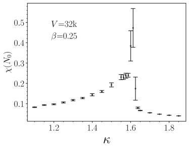
(a)

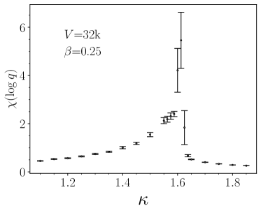
(b)

Figure 1: Susceptibility plots (a) $\chi_{N_{0}}$ and (b) $\chi_{\log{q}}$ for $V=32K$ are shown. The peaked structure near $\kappa\sim 1.6$ indicates a phase transition.

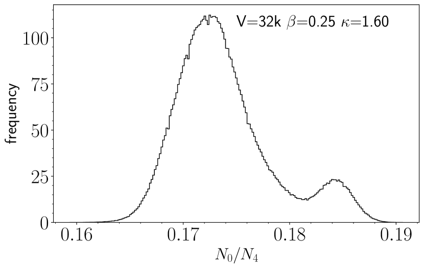
Figure 2: First order nature of the transition at $\beta=0.25$ can be see from the (a) Monte Carlo time series for $N_{0}/N_{4}$ and (b) double peak structure of the probability density of $N_{0}/N_{4}$.

The partition function of the model for the pure gravity takes the form

$$Z=\sum_{T}\rho(T)e^{-S}$$ (1)

where the discrete action $S$ is given by

$$S=-\kappa N_{0}+\lambda N_{4}+\gamma(N_{4}-V)^{2},$$ (2)

where the sum runs over all abstract triangulations with fixed (here spherical) topology  The first two terms in the action depending on the number of vertices $N_{0}$ and the number of four simplices $N_{4}$ arise from using Regge calculus Regge (1961); Thorne et al. (2000) to discretize the continuum Einstein-Hilbert action with $\kappa$ playing the role of the bare Newton constant and $\lambda$ a bare cosmological constant. The third term plays an auxiliary role in effectively fixing the target volume to $V$ by tuning $\lambda$ while still allowing for small fluctuations $\delta V\sim\frac{1}{\sqrt{\gamma}}$.

The central assumption in this approach to quantum gravity is that the sum over triangulations reproduces, in some appropriate continuum limit, the ill-defined continuum path integral over metrics modulo diffeomorphisms. In two dimensions this prescription is known to reproduce known results for 2d gravity from Liouville theory and matrix models Boulatov et al. (1986); Kazakov (1986) but in higher dimensions it is merely a plausible ansatz.

The assumption of most recent works is that an additional measure term $\rho(T)$, which depends on local properties of the triangulation, is needed to ensure this correspondence with continuum gravity remains true Ambjørn et al. (2013); Laiho et al. (2017a). Here we employ a new form

$$\rho(T)=\prod_{i=1}^{N_{0}}q_{i}^{\beta},$$ (3)

where $q_{i}$ denotes the number of simplices sharing vertex $i$ and $\beta$ is a new parameter. This is similar to the local measure term used in previous studies Laiho et al. (2017a); Ambjørn et al. (2013). It is conjectured that tuning the coupling to such an operator is necessary to restore continuum symmetries and approach a fixed point where a continuum limit describing quantum gravity can be taken Ambjørn et al. (2013).

Our work is focused on examining the phase structure of the model in the $(\kappa,\beta)$ with the goal of searching for critical behavior and locating a region where such a continuum limit can be taken.

III Phase Structure

We employ a Monte Carlo algorithm to sample the sum over random triangulations Catterall (1995). Five elementary local moves (“Pachner moves”) which, iterated appropriately are known to be sufficient to reach any part of the triangulation space.

Two of the simplest observables that can be used to locate the transition are the node and measure susceptibilities which are defined by

$$\chi_{N_{0}} =\frac{1}{V}\left(\left\langle N_{0}^{2}\right\rangle-\left\langle N_{0}\right\rangle^{2}\right)$$ (4)

$$\chi_{\ln{q}} =\frac{1}{V}\left(\left\langle Q^{2}\right\rangle-\left\langle Q\right\rangle^{2}\right)$$ (5)

with $Q=\frac{1}{N_{0}}\sum_{i=1}^{N_{0}}\ln{q_{i}}$. In fig 1 we show these as a function of $\kappa$ at $\beta=0.25$ for a lattice of (average) volume $N_{4}=32,000$. The peak in both quantities indicates the presence of a phase transition.

In fig. 2 we show the Monte Carlo time evolution of the vertex number $N_{0}$ and its associated probability distribution for a $V=32,000$ simplex simulation close to the critical line at $\beta=0.25$. The tunneling behavior in the Monte Carlo time series together with the double peak structure in the probability distribution for the number of vertices $P(N_{0})$ constitute strong evidence that the transition is first order in this region. This precludes a continuum limit and indeed the observation of a similar structure at $\beta=0$ was the original motivation for introducing a measure term.

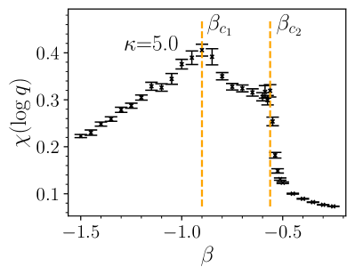
Figure 3: At large $\kappa$ two distinctive peaks are observed in the susceptibility plots. Position of the critical points are shown with the vertical lines.

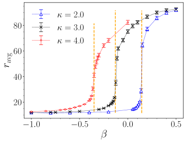
Figure 4: $\beta$ dependence of the average radius $r_{\rm avg}$ at different fixed values of $\kappa$, at a target volume $V=32$K. Vertical lines denote the position of the critical points $\hat{\beta}_{c}$ at different Gravitational constants $\kappa$.

$\bm{\beta}$	$\bm{\kappa_{c}}$	$\bm{\hat{\kappa}_{c}}$
1.00	-0.89(1)	-0.894(6)
0.50	0.75(1)	0.756(6)
0.25	1.61(2)	1.606(6)
$\bm{\kappa}$	$\bm{\beta}_{c}$	$\bm{\hat{\beta}_{c}}$
2.0	0.14(1)	0.144(6)
2.5	0.00(1)	0.006(6)
3.0	-0.13(1)	-0.13(1)
3.5	-0.25(1)	-0.244(6)
4.0	-0.36(1)	-0.35(1)
4.5	-0.46(1)	-0.46(1)
5.0	-0.56(1)	-0.56(1)

Table 1: Pseudo-transition point $\kappa_{c}$ ($\beta_{c}$) obtained from fixed $\beta$ ($\kappa$) scan of the susceptibilities at target volume $V=32$ k vs corresponding estimates of the critical point $\hat{\kappa}_{c}$ ($\hat{\beta}_{c}$) determined from the average radius $r_{\rm avg}$.

As we increase $\kappa$ we observe that the latent heat of the transition, as measured by the separation in the two peaks in the probability distribution $P(N_{0})$ decreases and the structure of the susceptibility plots changes. If one fixes $\kappa$ one observes a broad peak centered at $\beta_{c1}$ followed by a much narrower peak at $\beta_{c2}$ with $\beta_{c2}>\beta_{c1}$, Fig. 3. For $\beta>\beta_{c2}$ the system is clearly in the branched polymer phase while for $\beta<\beta_{c1}$ the system is clearly in the crumpled phase. The separation $\Delta\beta$ between the two critical points narrows down as the volume is increased. In our work we have used $\beta_{c2}$ as our best estimate for the true critical point $\beta_{c}$.

To complement this determination of the critical point we have also studied the mean radius of the discrete geometry. This is defined by

$$r_{\mathrm{avg}}=\frac{1}{N_{4}}\left\langle\sum_{r}r\,N_{3}(r)\right\rangle_{T},$$ (6)

where $N_{3}(r)$ is the number of four-simplices at geodesic distance $r$ measured on the dual lattice from some randomly chosen origin. In fig. 4 we show a plot of the mean radius $r_{\rm avg}$ vs $\beta$ for several values of $\kappa$. The phase transition visible in the susceptibilities is clearly also seen in $r_{\rm avg}$. To find the critical coupling, we computed a numerical derivative of the radius as a function of $\beta$ and identified the critical point $\hat{\beta}_{c}$ as the point where this derivative is maximal. A list of transition points derived from this observable are listed in the second column of the table 1 and shown to agree very well with the value $\beta_{c}$ determined from the $\chi(N_{0})$ and $\chi_{\log{q}}$ susceptibilities. Notice for small $\kappa$ we have fixed $\beta$ and scanned the transition in $\kappa$ while for large $\kappa$ we have fixed $\kappa$ and done a scan in $\beta$ values.

IV Hausdorff dimension

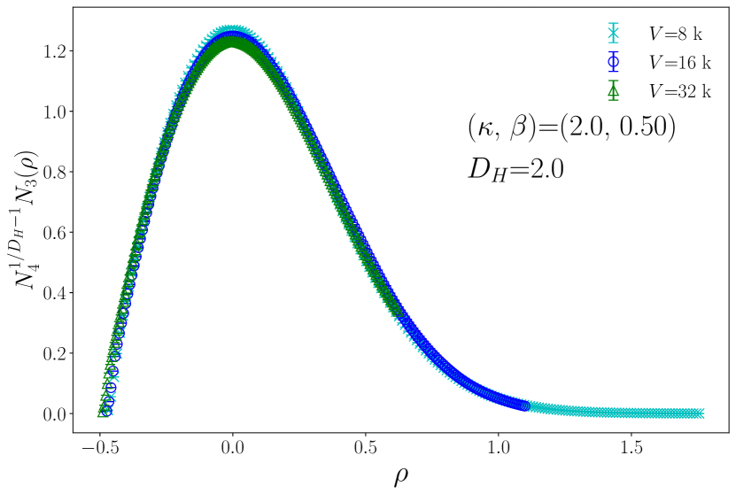
Figure 5: Data collapse of the three volume $N_{3}(\rho)$ with scaled distance is consistent with $D_{H}=2.0$ in the BP phase.

To compute the Hausdorff dimension $D_{H}$ we assume that $N_{3}(r)$ takes the scaling form

$$N_{3}(r)=N_{4}^{1/D_{H}-1}f\left(r/N_{4}^{1/D_{H}}\right).$$ (7)

Fitting to this form shows that the Hausdorff dimension in the branched polymer phase is consistent with the value of $D_{H}=2$ (Fig. 5) while in the collapsed phase, the extracted value of $D_{H}$ from such fits is large which is consistent with the continuum expectation of infinite $D_{H}$ Ambjørn and Jurkiewicz (1995); Coumbe and Laiho (2015). At small distances, $N_{3}$ should grow as $\sim r^{D_{H}-1}$ Ambjørn and Jurkiewicz (1995). In practice we have used this fact rather than data collapse on the scaling form to extract $D_{H}$ close to the critical line on our largest lattice by fitting

$$N_{3}=A\,r^{D_{H}-1}+B.$$ (8)

Fig 6 shows such a fit. The results presented are an ensemble average computed from 2000 thermalized configurations. The fit is performed at several fixed $\beta$ and fixed $\kappa$ to observe the variation in the Hausdorff dimension as we moved from the collapsed phase to the branched polymer phase. The value of the Hausdorff dimension is strongly influenced by the distance from the critical line as can be seen in Fig. 7 which shows $D_{H}(\beta)$ at a fixed $\kappa=4.0$. From the rise of the value of DH towards the left, it is evident that as we probe deep into the collapsed phase, we get larger Hausdorff dimensions. Also clearly visible is the fact that deep in the BP phase on the right of the diagram the value approaches the known value of $D_{H}=2$.

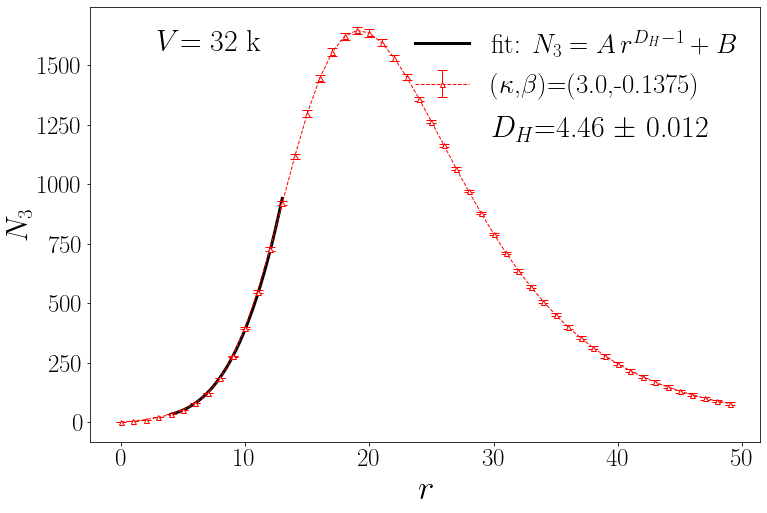
Figure 6: Fit of three volume data at small distance.

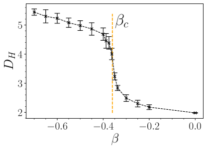
Figure 7: Variation in Hausdorff dimension $D_{H}$ with $\beta$ at $\kappa=4.0$ at $V=32$ K. Position of the critical coupling $\beta_{c}$ derived from susceptibility is noted with the vertical line.

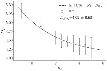
Figure 8: Fit of extracted Hausdorff dimension $D_{H}$ as a function of critical coupling along transition line.

The value of $D_{H}$ along the critical line is shown in fig. 8 which also includes a fit of the form

$$D_{H}=M/(\kappa+B)+D_{H,\infty}.$$ (9)

Here, $M$ and $B$ are fit parameters and $D_{H}\to D_{H,\infty}$ as $\kappa\to\infty$. We find $D_{H,\infty}=4.06\pm 0.64$ which is consistent with the emergence of four dimensional de Sitter space in this limit.

Encouraged by this we have compared our three-volume distribution near the critical point at large $\kappa$ with the (Euclidean) de-Sitter solution . The associated three volume profile for the Wick rotated case takes the form of Eqn. 10 Ambjørn et al. (2008); Glaser and Loll (2017); Laiho et al. (2017a). This is shown in Fig. 9 and indicates that the average geometry at small to intermediate distances is indeed consistent with de Sitter as $\kappa$ gets large.

$$N_{3}(r)=\frac{3}{4}N_{4}^{3/4}\Gamma\cos^{3}\left(\frac{r-b}{s_{0}N_{4}^{1/4}}\right)$$ (10)

Here, $s_{0}$, $\Gamma$ and $b$ are fit parameters. One can think of $s_{0}$ as determining a relative lattice spacing for different values of the $(\kappa,\beta)$. We find good matching of our data to the de-Sitter solution starting from a small distance $r$ up to about five steps beyond the maxima. The long tail of the distribution is likely a finite size effect Laiho et al. (2017a).

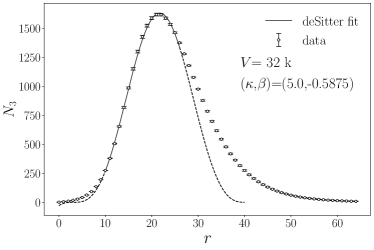
Figure 9: Fit to the de-Sittter solution of the three volume distribution data.

V Spectral Dimension

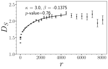
Figure 10: Sample fit of the spectral dimension near the transition line in the phase space.

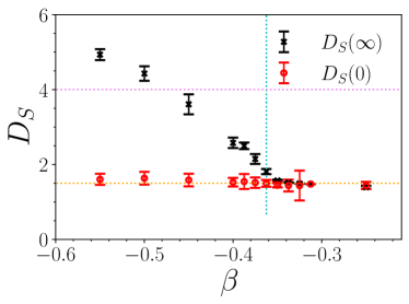
Figure 11: UV ($D_{S}(0)$) and IR ($D_{S}(\infty)$) spectral dimension across transition at a fixed $\kappa=4.0$. Vertical line denotes the position of the transition point and the two horizontal line denotes the $D_{s}$ value of 1.5 and 4 for comparison with the data.

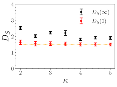
Figure 12: UV ($D_{S}(0)$) and IR ($D_{S}(\infty)$) spectral dimension along the the transition line. Horizontal line denotes the $D_{s}$ value of 1.5 for the comparison.

Another measure of dimension for a fluctuating geometry is called the “spectral dimension” $D_{S}$. It can be computed for a simplicial manifold $\mathcal{M}$ using a random walk process. Starting from a randomly selected simplex the random walk corresponds to successively moving from one simplex to one of its neighbors via a randomly selected face. This process is then iterated a large number of times. To compute the spectral dimension one records the number of times the walk returns to the starting simplex as a function of the diffusion time (number of steps of the random walk). By running several of these walks and averaging over starting points and over the ensemble of configurations obtained at some fixed $\beta$ and $\kappa$ we can obtain the probability of returning to the starting simplex $P_{r}(\sigma)$ after $\sigma$ steps. The spectral dimension is then defined from the relation:

$$D_{S}(\sigma)=-2\frac{d\log\left\langle P_{r}(\sigma)\right\rangle}{d\log\sigma}$$ (11)

The return probability itself is a useful quantity which can be used to find the relative lattice spacing at different points on the transition line Laiho et al. (2017a). This is discussed in more detail in appendix A.

In the branched polymer phase we observe $D_{S}=4/3$ which is consistent with theoretical expectations Jonsson and Wheater (1998) while in the crumpled phase it is large. At the critical point we find $D_{S}$ is not well fitted by a constant but instead runs with scale $\sigma$. In fig. 10 we show a plot of this running spectral dimension for $V=32K$ and $\beta=-0.1375,\,\,\kappa=3.0$.

We used 2000 thermalized configurations for the computation of the spectral dimension. Each random walk is performed up to 15000 steps and we choose 32000 randomly chosen sources per configuration. The fit is attempted over different ranges. Due to the finite volume of the lattices, the spectral dimension will increase and reach a maximum before decreasing. However, the number of steps needed to reach this maximum depends on the effective dimension of the manifold. We attempted to fit our data up to this maximum whenever possible. This amounts to choosing different fit ranges at different regions of the parameter space. The choice of the fit range can be justified by tracking the p-value of the fits.

As in previous works Ambjørn et al. (2005); Laiho et al. (2017a), we found the following fit function best represents the data

$$D_{S}(\sigma)=a+\frac{b}{c+\sigma}.$$ (12)

The fit function yields estimates for the spectral dimension at small distances $D_{S}(0)$ and also at large distances $D_{S}(\infty)$. A single elimination jackknife procedure is used to compute the error-bar, and the fit is performed for different fit ranges. Systematic errors due to the choice of the fit range are added in quadrature with the statistical error of the best fit used to compute the overall error. We use the metric ‘p-value’ to select reasonable fit ranges for the data. Fig. 11 shows the variation of $D_{S}(0)$ and $D_{S}(\infty)$ across the transition line from the crumpled to the branched polymer phase, while Fig. 12 shows the variation of these quantities along the transition line. Clearly $D_{S}$ runs to small ($D_{S}\sim 1.5$) values in the UV which is consistent with the earlier EDT studies Laiho et al. (2017b), and CDT studies Coumbe and Jurkiewicz (2015). In the IR regime the spectral dimension $D_{S}(\infty)$ is larger with $D_{S}(\infty)$ varying from $1.82-2.52$. This scale dependence of the spectral dimension was also seen earlier in CDT Ambjørn et al. (2005), renormalization group approach Lauscher and Reuter (2005), loop quantum gravity Modesto (2009) and in string theory models Hořava (2009). It is not clear from our study whether the UV spectral dimension $D_{S}(\infty)$ attains larger values for larger $N_{4}$. Larger volume simulations with combinatorial triangulations must be conducted to resolve the tension in $D_{S}(\infty)$ with the results obtained from the degenerate combinatorial calculations Laiho and Coumbe (2011) 

VI Conclusions

We have explored the phase diagram of combinatorial Euclidean dynamical triangulation models of four dimensional quantum gravity. Our model contains two parameters - a bare gravitational coupling $\kappa$ and a measure parameter $\beta$. We find evidence for a critical line $\kappa_{c}(\beta)$ dividing a crumpled phase from a branched polymer phase in agreement with earlier work Ambjørn et al. (2013); Laiho et al. (2017a). While this line is associated with first order phase transitions for small $\kappa$ this transition softens with increasing coupling. An intermediate “crinkled” phase opens up in this regime but we have focused our attention on the boundary between this region and the branched polymer phase in our analysis since this is the only place where we have observed consistent scaling that survives the large volume limit. When we refer to the critical point in our results we always mean the boundary between the crinkled and branched polymer phases.

The focus of much of our work has been to compute the Hausdorff and spectral dimensions as we approach this critical line from the crumpled phase. We find evidence that the Hausdorff dimension $D_{H}$ along the critical line approaches $D_{H}=4$ as $\kappa$ increases where it is possible to obtain increasingly good fits to to classical de Sitter space. The spectral dimension $D_{S}(s)$ is observed to run with scale $s$ attaining values consistent with $D_{S}(0)=\frac{3}{2}$ at short distances for all values of $\kappa$. These results are consistent with earlier work using degenerate triangulations and causal dynamical triangulation models and models using different measure terms Ambjørn et al. (2013); Laiho et al. (2017a); Coumbe and Jurkiewicz (2015). However our measurement of the spectral dimension at long distances $D_{s}(\infty)$ barely exceeds $D_{s}(\infty)\sim 2$. This result is somewhat in tension with the earlier work. However, we show that $D_{s}(\infty)$ depends strongly on the distance in parameter space from the critical line which renders such measurements delicate and may explain this discrepancy. Large finite volume effects which have been observed in earlier studies may also make this measurement difficult.

Appendix A Relative lattice spacing

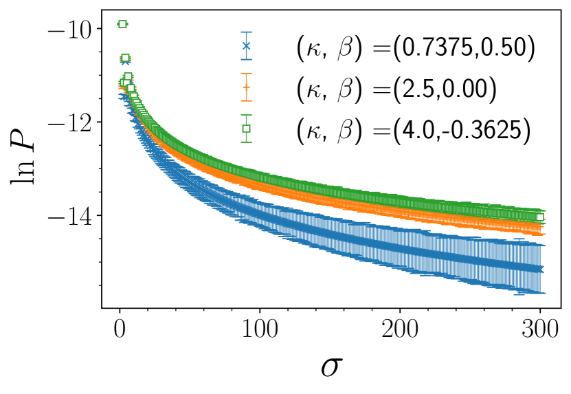
(a)

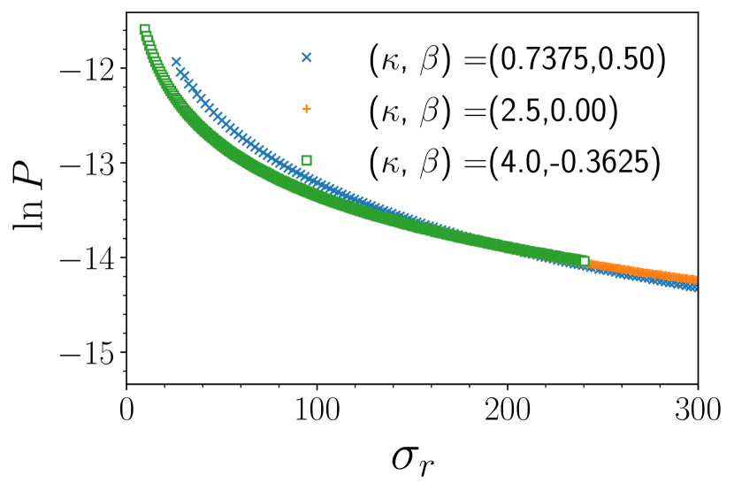
(b)

Figure 13: Return probability at different points in the critical line at lattice volume $V=32$ k (a) with respect to diffusion step ($\sigma$), (b) with respect to rescaled diffusion step ($\sigma_{r}$). The scaling allows to find relative lattice spacing along the transition line. Associated error-bars are not shown in the right-hand figure to demonstrate the superimposed data from different points in the transition line.

$\kappa_{c}$	-0.90	-0.7375	1.5625	2.0	2.5	3.0	3.5	4.0	4.5	5.0
$a_{r}$	1.5	1.475	1.135	1.05	1	0.935	0.92	0.895	0.87	0.86

Table 2: Relative lattice spacing along the transition line as $\kappa$ is varied.

In this work, we did not attempt to perform a precise measurement of the renormalized gravitational constant which determines the absolute lattice spacing. Two different methods of finding the gravitational constant in the context of the Euclidean dynamical triangulation can be found in the two recent papers by Laiho et.el. Dai et al. (2021b); Bassler et al. (2021). We have used the relative lattice spacing as obtained from the return probability in our work. In fig. 13(a) we show the return probability at several different points along the critical curve for $V=32$ K and in fig. 13(b) and show how these curves can be collapsed onto a single curve by rescaling the step size $\sigma$. Rescaling of the step $\sigma=\sigma_{r}a_{r}^{2}$ can be interpreted as yielding a relative lattice spacing $a_{r}$ as $\kappa$ varies along the critical curve. Values of the relative lattice constant $a_{r}$ are noted in the Table 2 and are consistent with the previous work by Laiho et. el.. Namely they reveal that as $\kappa$ approaches infinity the corresponding lattices get finer Laiho et al. (2017a). Hence, for a fixed target volume $V$, the physical volume is smaller at larger $\kappa_{c}$ and it is likely that the results obtained would suffer greater finite size effect in that region.

References

- Ashtekar and Bianchi (2021) A. Ashtekar and E. Bianchi, Reports on Progress in Physics (2021).
- Loll (2019) R. Loll, Classical and Quantum Gravity 37, 013002 (2019).
- Weinberg (1979) S. Weinberg, General relativity, (1979).
- Niedermaier and Reuter (2006) M. Niedermaier and M. Reuter, Living Reviews in Relativity 9, 5 (2006).
- Ambjorn et al. (2013) J. Ambjorn, A. Görlich, J. Jurkiewicz, and R. Loll, International Journal of Modern Physics D 22, 1330019 (2013).
- Laiho and Coumbe (2011) J. Laiho and D. Coumbe, Physical Review Letters 107, 161301 (2011), arXiv: 1104.5505.
- Laiho et al. (2017a) J. Laiho, S. Bassler, D. Coumbe, D. Du, and J. T. Neelakanta, Physical Review D 96, 064015 (2017a), arXiv: 1604.02745.
- Dai et al. (2021a) M. Dai, J. Laiho, M. Schiffer, and J. Unmuth-Yockey, Physical Review D 103, 114511 (2021a).
- (9) S. Bassler, J. Laiho, M. Schiffer, and J. Unmuth-Yockey, , 12.
- Ambjørn et al. (2013) J. Ambjørn, L. Glaser, A. Görlich, and J. Jurkiewicz, Journal of High Energy Physics 2013, 100 (2013).
- Catterall et al. (1996) S. Catterall, J. Kogut, R. Renken, and G. Thorleifsson, Physics Letters B 366, 72 (1996).
- Ambjørn and Jurkiewicz (1994) J. Ambjørn and J. Jurkiewicz, Physics Letters B 335, 355 (1994).
- Regge (1961) T. Regge, Il Nuovo Cimento (1955-1965) 19, 558 (1961).
- Thorne et al. (2000) K. S. Thorne, C. W. Misner, and J. A. Wheeler, Gravitation (Freeman San Francisco, 2000).
- Boulatov et al. (1986) D. Boulatov, V. Kazakov, I. Kostov, and A. A. Migdal, Nuclear Physics B 275, 641 (1986).
- Kazakov (1986) V. A. Kazakov, Physics Letters A 119, 140 (1986).
- Catterall (1995) S. Catterall, Computer Physics Communications 87, 409 (1995).
- Ambjørn and Jurkiewicz (1995) J. Ambjørn and J. Jurkiewicz, Nuclear Physics B 451, 643 (1995).
- Coumbe and Laiho (2015) D. Coumbe and J. Laiho, Journal of High Energy Physics 2015, 1 (2015).
- Ambjørn et al. (2008) J. Ambjørn, A. Görlich, J. Jurkiewicz, and R. Loll, Physical Review D 78, 063544 (2008).
- Glaser and Loll (2017) L. Glaser and R. Loll, Comptes Rendus Physique 18, 265 (2017).
- Jonsson and Wheater (1998) T. Jonsson and J. F. Wheater, Nuclear Physics B 515, 549 (1998).
- Ambjørn et al. (2005) J. Ambjørn, J. Jurkiewicz, and R. Loll, Physical review letters 95, 171301 (2005).
- Laiho et al. (2017b) J. Laiho, S. Bassler, D. Coumbe, D. Du, and J. Neelakanta, arXiv preprint arXiv:1701.06829 (2017b).
- Coumbe and Jurkiewicz (2015) D. N. Coumbe and J. Jurkiewicz, Journal of High Energy Physics 2015, 151 (2015), arXiv: 1411.7712.
- Lauscher and Reuter (2005) O. Lauscher and M. Reuter, Journal of High Energy Physics 2005, 050 (2005).
- Modesto (2009) L. Modesto, Classical and Quantum Gravity 26, 242002 (2009).
- Hořava (2009) P. Hořava, Physical review letters 102, 161301 (2009).
- Dai et al. (2021b) M. Dai, J. Laiho, M. Schiffer, and J. Unmuth-Yockey, Physical Review D 103, 114511 (2021b).
- Bassler et al. (2021) S. Bassler, J. Laiho, M. Schiffer, and J. Unmuth-Yockey, Physical Review D 103, 114504 (2021).