Cross-Skeleton Interaction Graph Aggregation Network for Representation Learning of Mouse Social Behaviour

Abstract

Automated social behaviour analysis of mice has become an increasingly popular research area in behavioural neuroscience. Recently, pose information (i.e., locations of keypoints or skeleton) has been used to interpret social behaviours of mice. Nevertheless, effective encoding and decoding of social interaction information underlying the keypoints of mice has been rarely investigated in the existing methods. In particular, it is challenging to model complex social interactions between mice due to highly deformable body shapes and ambiguous movement patterns. To deal with the interaction modelling problem, we here propose a Cross-Skeleton Interaction Graph Aggregation Network (CS-IGANet) to learn abundant dynamics of freely interacting mice, where a Cross-Skeleton Node-level Interaction module (CS-NLI) is used to model multi-level interactions (i.e., intra-, inter- and cross-skeleton interactions). Furthermore, we design a novel Interaction-Aware Transformer (IAT) to dynamically learn the graph-level representation of social behaviours and update the node-level representation, guided by our proposed interaction-aware self-attention mechanism. Finally, to enhance the representation ability of our model, an auxiliary self-supervised learning task is proposed for measuring the similarity between cross-skeleton nodes. Experimental results on the standard CRMI13-Skeleton and our PDMB-Skeleton datasets show that our proposed model outperforms several other state-of-the-art approaches.

I Introduction

THE analysis of rodent social behavior is an interesting issue in neuroscience and pharmacology. Laboratory mice provide a valuable platform to study psychiatric and neurological disorders such as Huntington’s [1], Alzheimer’s [2], schizophrenia [3], as well as Parkinson’s disease [4]. In this paper, we only discuss the case of Parkinson’s disease. Traditionally, social behaviour identification is performed by manually annotating hours of video recordings of interactions between mice with pre-defined behaviour labels. Unfortunately, this human labeling practice is time-consuming, error-prone and highly subjective. Recent advances in computer vision and pattern recognition have facilitated automated analysis of complex animal behaviours [5, 6, 7, 8], which provides another dimension to understand the relationship between neural activities and behavioural phenotypes in neuroscience research.

As more and more accurate results have been provided by deep learning based pose estimation models [9, 10, 11, 12], researchers have started to directly recognise mouse social behaviours using pose information (i.e., the locations of keypoints generated by pose estimators) [7, 13]. Compared with RGB features, pose information includes only 2D or 3D positions of keypoints, which may be free of environmental noise (e.g. complex background and illumination changes) [14]. However, the features extracted by most of the existing systems are hand-crafted, based on pre-defined keypoints. For instance, in [13], we investigated the distance relations between two noses (i.e., distance feature) calculating the distance between the noses of two mice. Actually, such hand-crafted shallow features are insufficient to describe the dependency between the corresponding keypoints. To this end, we need to develop an effective way to automatically model the spatio-temporal interactions between keypoints.

Graph convolutional networks (GCNs) [15], which generalise convolution from images to graphs, have been successfully adopted in many areas to model graph-structured data, especially in skeleton based human action recognition approaches [16, 17, 18]. Nevertheless, most of GCN-based methods have been designed for action recognition of single objects rather than multiple interacting subjects. In most of these established models, a standard human skeleton with all joints is utilised to model the potential spatio-temporal dependencies between the joints. To capture discriminative action features, multi-view solutions [19] consisting of two ensemble models with different skeleton typologies are developed to utilise comprehensive information. Although such approach can significantly improve the discriminative capability, the two sub-models need to be trained independently - how to select a new and effective skeleton topology is difficult to determine. Moreover, to obtain the graph-level representation that represents a specific action, global average pooling (GAP) [20] is normally used to aggregate node-level representation from the final stage of the network. However, this operation processes all node features equally without considering the importance of different nodes, structural constraints and dependencies between them.

We here propose a Cross-Skeleton Interaction Graph Aggregation Network (CS-IGANet) to effectively learn abundant interaction relationships between mice, shown in Fig. 1. To explore complex social interactions between mice, we first introduce dense and sparse skeletons to describe diverse spatial structures of a mouse, shown in Fig. 1(a). Here, mouse skeleton refers to a list of keypoint connections [21]. Then, a novel Cross-Skeleton Node-level Interaction (CS-NLI) module, shown in Fig. 1(b), is proposed to model the intra- (between keypoints of each mouse), inter- (between keypoints of different mice) and cross-skeleton (between keypoints of different skeletons) interactions in an unified way, allowing us to discover abundant dynamic relations of social interactions. For each skeleton branch, a GCN-based module [20] is first adopted to model the intra-skeleton interaction of each mouse based on the extracted keypoints, before we fuse dense geometric properties and velocity information for multi-order dense information fusion. Afterwards, we model the social interactions of mice, where an adaptive inter-skeleton interaction matrix is formulated to integrate the motion information from two or more interactive mice. Similarly, we further explore the cross-skeleton interactions of these mice.

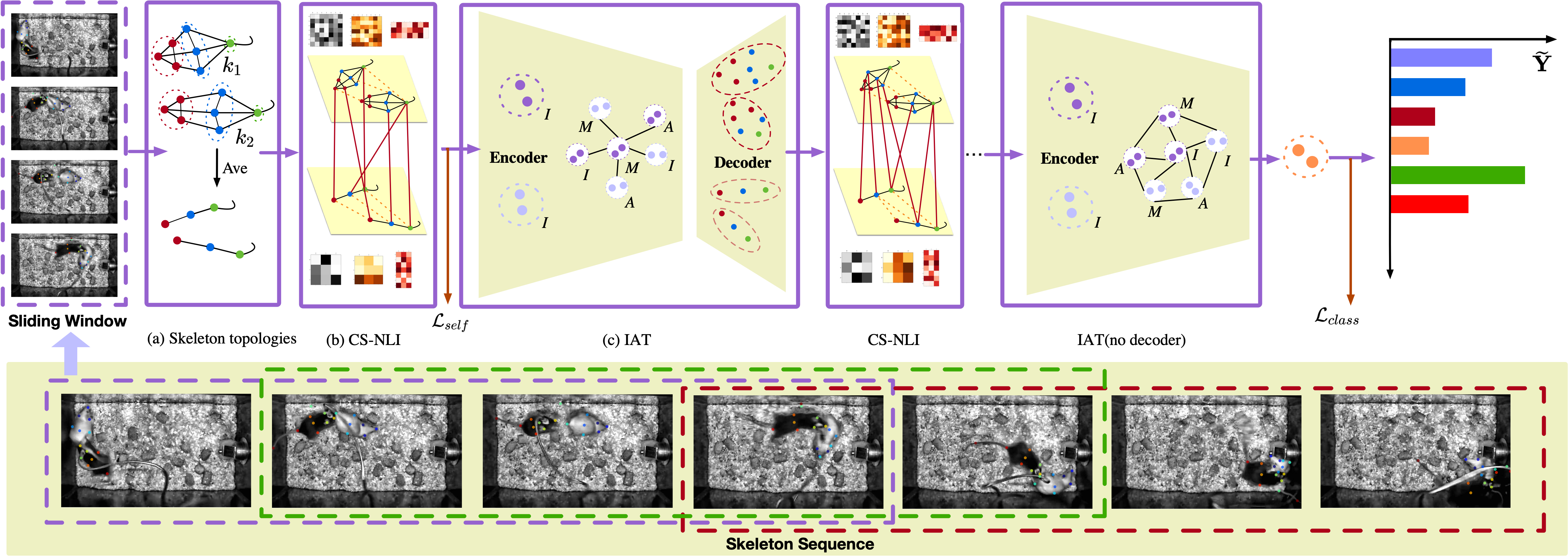
Figure 1: Overview of the proposed CS-IGANet for mouse social behaviour representation learning. (a) The skeleton topologies of two mice. The input is a skeleton sequence from a long video, where each sliding window centered at a certain frame contains a specific behaviour [6]. We define dense and sparse skeletons for describing diverse spatial structures of a mouse (Ave - average). (b) Cross-Skeleton Node-level Interaction (CS-NLI) module. It is composed of intra-skeleton (black solid lines and interaction matrix), inter-skeleton (yellow dashed lines) and cross-skeleton (red solid lines) interactions with the ability to reveal powerful node-level representation of social interactions (see Section III-A). (c) Interaction-aware Transformer (IAT). For each skeleton branch, the node-level representation encoded by (b) is hierarchically aggregated to generate graph-level representation $I$ (The two dark purple circles represent the graph-level representations of two mice from the dense skeleton). In the encoder, we further fuse different representations ($I$, $M$ and $A$) to enhance graph-level representation (see Section III-B1). The decoder aims to adaptively update the node-level representation. (see Section III-B2). $\mathcal{L}_{class}$ is the cross-entropy loss, and $\mathcal{L}_{self}$ denotes the self-supervised loss (see Section III-C).

We also propose a novel Interaction-Aware Transformer (IAT) to dynamically learn graph-level representation of social behaviour, and update the node-level representation used as the input to the next layer, which is guided by the proposed interaction-aware self-attention unit, shown in Fig. 1(c). The encoder aims at mining behaviour-related interaction saliency (i.e., conspicuous nodes) based on intra- and inter-skeleton interactions, where the node-level representation is used to generate multiple subgraphs and the last one denotes the graph-level representation of social behaviour. Afterwards, such graph-level representations from different skeletons are integrated with representations generated by trivial pooling methods (e.g., average [20], max [22]) to enhance the graph-level representation. The decoder is designed so as to adaptively update the node-level representation via the proposed interaction-aware self-attention unit.

We believe that there exists meaningful similarity between the dense and sparse skeletons that both describe spatial configurations of a mouse. To better preserve these attributes within the cross-skeleton pairwise nodes, we design an auxiliary self-supervised learning module. By jointly optimising the self-supervised objective function and the traditional classification loss function (i.e., cross-entropy loss), our proposed model can yield more discriminative representation.

The main contributions can be summarised as follows:

• We propose a novel Cross-Skeleton Interaction Graph Aggregation Network (CS-IGANet) to learn mouse social behaviour representation, where dense and sparse skeletons cooperatively explore the spatio-temporal dynamics of social interactions.

• The proposed Cross-Skeleton Node-level Interaction (CS-NLI) module is able to engender powerful node-level representation by modelling multi-level interactions of mice, i.e., intra-, inter- and cross-skeleton interactions, where multi-order dense information are fused for inferring corresponding interaction patterns.

• The proposed Interaction-Aware Transformer (IAT) allows for dynamic updating of graph- and node-level representation. This can be achieved by designing an encoder-decoder architecture, where the former hierarchically aggregates node-level representation for graph-level representation learning whilst the latter adaptively update node-level representation for extracting higher-level features.

• We introduce an auxiliary self-supervised learning strategy to enable the proposed model to focus on the similarity between pairwise nodes from different skeletons, so as to enhance the representation ability of our model.

II Related Work

II-A Pose-based Mouse Social Behaviour Recognition

There are few works studying mouse social behaviours through pose analysis. For example, [23] constructed a spatio-temporal feature vector composed of 13 measurements (e.g., relative position, shape and movement) based on the tracking results of the proposed tracker, and then applied random decision trees to classifying those extracted features. Similarly, [7] detected the nose, head, body and tail of each mouse using the standard YOLOv3 network, based on the extracting features such as distance between the body centers. However, these extracted features are shallow with limited spatio-temporal representation.

Thanks to pose estimation models [9, 10, 11], people directly adopted the results of pose estimators to conduct downstream tasks such as behaviour recognition. [13] reported SimBa that analyses mouse social behaviours based on the pose estimation tracking results, where a random forest algorithm was leveraged to classify behavioural patterns. However, the 490 features (e.g. area of mouse convex hull, distance between part1 and part2) in their system are still shallow. Similar to SimBa, [24] also introduced a system called MARS for the analysis of social behaviors, whereas 270 keypoint based spatio-temporal features were generated. However, these hand-crafted features cannot capture robust spatio-temporal relationships of keypoints, especially for complex social interactions.

II-B Skeleton-based Human Action Recognition

Graph Convolutional Networks (GCNs) [25, 20, 26, 27, 28, 29, 30] are prevalent for processing skeleton data due to their strong ability of capturing structural dependencies of joints. [25] exploited GCN for skeleton-based action recognition, and utilised the spatial temporal graph convolutional network (ST-GCN) to model the skeleton data as the graph structure. However, it uses a fixed skeleton graph and represents only the physical structure of the human body. [20] delineated a two-stream GCN model, i.e., 2s-AGCN to learn an adaptive graph where both the joint and bone information is explicitly utilised, significantly improving the model performance. [26] introduced a sophisticated feature extractor named MS-G3D, in which the disentangled multi-scale aggregator and G3D are used to eliminate redundant dependencies between neighborhoods and model spatio-temporal information interaction, respectively. [19] proposed a MV-IGNet network to formulate complementary action representations by adopting two pre-defined skeleton topologies. As we discussed above, it is difficult to determine a new and effective skeleton topology. Transformer [31] using self-attention has also been applied to graph-structured data modelling due to its powerful ability of modelling long-range dependencies [32, 27, 33]. Although most of the aforementioned approaches have produced promising results in skeleton-based human action recognition, they mainly focus on single-object action without modelling the interactions between objects, and hence lack the ability to generalise social representations.

III Proposed Methods

The skeleton sequence of $K$ mice with $T$ frames and $N$ keypoints can be represented as a spatio-temporal graph $\mathcal{G}=(\mathcal{V},\mathcal{E},\mathcal{X})$. $\mathcal{V}=\left\{v_{t,n,k}\mid t,n,k\in\mathbb{Z},1\leq t\leq T,1\leq n\leq N,1\leq k\leq K\right\}$ is the set of all the nodes $v_{t,n,k}$ of the mouse skeleton graph, i.e., keypoints of the skeleton over all the time sequence. $\mathcal{E}$ represents the edge set consisting of two subsets, i.e., spatial topology $\mathcal{E_{S}}=\left\{(v_{t,n,k},v_{t,m,k})\mid 1\leq t\leq T,1\leq n,m\leq N,1\leq k\leq K\right\}$ that describes the relationship between any pair of keypoints $(v_{n},v_{m})$ of mouse $k$ at time $t$, and temporal topology $\mathcal{E_{T}}=\left\{(v_{t,n,k},v_{t+1,n,k})\mid,1\leq t\leq T,1\leq n\leq N,1\leq k\leq K\right\}$ indicating the relationship between keypoints along consecutive time frames. $\mathcal{E_{S}}$ of each mouse at time $t$ can be formulated as an adjacency matrix $\textbf{A}\in\mathbb{R}^{N\times N}$ where initial element $a_{n,m}\in\left\{0,1\right\}$ reflects the correlation strength between $v_{n}$ and $v_{m}$. $\mathcal{X}=\left\{x_{t,n,k}\mid 1\leq t\leq T,1\leq n\leq N,1\leq k\leq K\right\}$ is a node features set, which is represented as a matrix $\mathbf{X}\in\mathbb{R}^{C\times T\times N\times K}$ where $x_{t,n,k}=\mathbf{X}(:,t,n,k)\in\mathbb{R}^{C}$ is the $C$ dimensional feature vector for node $v_{t,n,k}$. In this work, we focus on skeleton-based mouse social behaviour recognition in long videos. During training, we wish to obtain a continuous behaviour sequence by the sliding window over the long video, where each window centered at a certain frame only contains one specific behaviour [6]. Hence, the behaviour sequence is represented as $\mathbb{X}=\left[\mathbf{X}^{(1)},\mathbf{X}^{(2)}\ldots,\mathbf{X}^{(B)}\right]\in\mathbb{R}^{B\times C\times T\times N\times K}$, where $B$ is the total number of sliding windows and $\mathbf{X}^{(B)}\in\mathbb{R}^{C\times T\times N\times K}$ is the feature set of the $B$-th window in the long video. Consequently, given $\mathbb{X}$, we aim to learn a non-linear prediction function to model the relationship between a sequence of the predicted labels (i.e., $\mathbb{Y}=\left[\mathbf{Y}^{(1)},\mathbf{Y}^{(2)}\ldots,\mathbf{Y}^{(B)}\right]$) and $\mathbb{X}$. In experiments, following the standard formulations [25, 20], we reshape the input sequence to $\mathbb{X}\in\mathbb{R}^{K\cdot B\times C\times T\times N}$ by moving $K$ to the batch dimension. Normally, for each sliding window, one behaviour is described as $A$ and $\mathbf{X}\in\mathbb{R}^{C\times T\times N}$, with $\mathbf{X}_{t}\in\mathbb{R}^{C\times N}$ being the node features at time $t$.

In this section, we will fully explain our proposed CS-NLI module that jointly models intra-, inter- and cross-skeleton interactions, our proposed IAT that dynamically creates graph-level representation and updates node-level representation, and the proposed auxiliary self-supervised learning strategy that encourages the proposed model to focus on the similarity between cross-skeleton pairwise nodes. The overview of our proposed framework is illustrated in Fig. 1.

III-A Cross-Skeleton Node-level Interaction

Mouse social behaviour recognition is non-trivial because it involves not only the individual behaviour but also the interactions between mice. Although the behavioural representation of each mouse on the both spatial and temporal domains can be interpreted by existing GCN-based network [20, 26, 19], they ignore the interaction between mice, which is crucial for fully learning the social behaviour representation. Therefore, in this section, we aim to explore the interaction between the keypoints of each mouse (i.e., intra-skeleton interaction) as well as interaction patterns between mice (i.e., inter-skeleton interaction) simultaneously. As aforementioned, we further model the spatio-temporal relationship between dense and sparse skeletons (i.e., cross-skeleton interaction) to learn skeleton-shared representations. The architecture of our proposed CS-NLI module is shown in Fig. 2.

III-A1 Intra-skeleton interaction modelling

Similar to [19, 34], we first construct $I$ types of skeleton sequences to learn behavioural information of mice. Following [21], we define the dense physical connections of all the keypoints. Then, we further design a sparse structure where keypoints in the same body part are aggregated into one keypoint by the averaging operation, as shown in Fig. 1(a). This is because some behaviours such as ‘approach’ can be understood based on the movements of keypoints from the sparse skeleton without knowing the exact locations of each keypoint (e.g., left and right ears).

To model the intra-skeleton interaction of mice (without loss of generality, we use two mice in this paper), we adopt the GCN-TCN structure shown in [20] to encode the spatio-temporal representation (more details about this model can be found in Supplementary A). We adopt the standard GCN to extract spatial features from the structural node connections due to its flexibility on skeleton modelling. TCN is then used to extract temporal features from skeleton sequences. A residual connection is also added for both GCN and TCN. Mathematically, given the skeleton sequence $\mathbf{X}_{s_{i}}^{l}\in\mathbb{R}^{C_{l}\times T_{l}\times N_{s_{i}}},\forall i\in\left\{1,2,\cdots,I\right\}$, where $s_{i}$ and $N_{s_{i}}$ denote the $i$-th skeleton and the number of the nodes in this skeleton, we define such interaction as follows:

$$\small\begin{split}\begin{aligned} \mathbf{X}_{s_{i}}^{(l+1)}&=\mathbf{\Gamma}(\Phi(\mathbf{X}_{s_{i}}^{l}))+\mathbf{X}_{s_{i}}^{l}\\ &=\mathbf{\Gamma}(\sum_{k}^{K_{v}}\mathbf{W}_{k}\mathbf{X}_{s_{i}}^{l}\left(\mathbf{A}_{k}+\mathbf{B}_{k}+\mathbf{C}_{k}\right)+\mathbf{X}_{s_{i}}^{l})+\mathbf{X}_{s_{i}}^{l}\end{aligned}\end{split}$$ (1)

where $\Phi(\cdot)$ and $\Gamma(\cdot)$ represent spatial and temporal modelling, respectively. The input $\mathbf{X}_{s_{i}}^{l}$ in $\Phi(\cdot)$ is reshaped to $\mathbb{R}^{C_{l}\cdot T_{l}\times N_{s_{i}}}$ by assigning $T_{l}$ as the channel dimension, and is then projected back to $\mathbb{R}^{C_{l}\times T_{l}\times N_{s_{i}}}$ for temporal convolution. We can obtain the intra-skeleton interaction by stacking multiple residual GCN and TCN modules. The output of such interaction in the $l$-th layer of our network is represented as $\mathbf{X}_{s_{i}}^{intra,l}$.

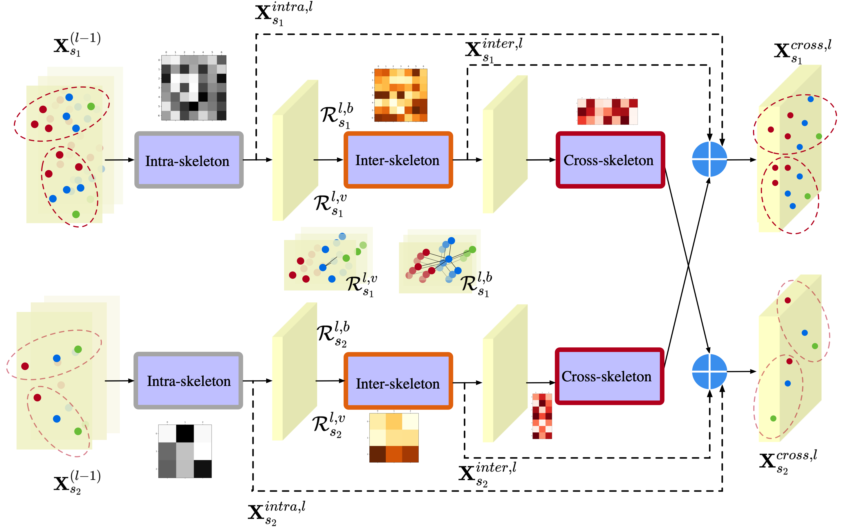
Figure 2: Architecture of the Cross-Skeleton Node-level Interaction module (CS-NLI). The inputs are node-level representations (circles with different colors) of the dense and sparse skeletons in the $(l-1)$-th layer, and each input contains the features of the mice. For each branch, $\mathbf{X}_{s_{i}}^{intra,l}$, $\mathbf{X}_{s_{i}}^{inter,l}$ and $\mathbf{X}_{s_{i}}^{cross,l}$ can be calculated by Eqs. (1), (10) and (12), respectively. This architecture is flexible and can be extended to deal with more skeletons and social behaviour recognition with more objects.

III-A2 Inter-skeleton interaction modelling

Based on the high-level features extracted using a sequence of residual GCN and TCN modules defined in Eq. (1), we then explore the interaction pattern between mice where the inter-skeleton interaction matrix, i.e., $\mathbf{A}_{k_{i}\rightarrow k_{j}}^{l}$, needs to be derived (for two mice, we have $\mathbf{A}_{k_{1}\rightarrow k_{2}}^{l}$ and $\mathbf{A}_{k_{2}\rightarrow k_{1}}^{l}$). We first explicitly embed both geometric distance and velocity information into the representation encoded by keypoint information because they carry behaviour-related features [19, 20, 17]. In particular, mouse body is highly deformable and most mouse behaviours have a relatively short duration. Unlike these approaches, we here extract dense geometric distance (Eq. (2)) and velocity information (Eq. (3)) simultaneously. For the node $v_{m}$ at the $l$-th layer of our network, we consider the relative positions between it and all the remaining nodes to construct a dense geometric distance set $\mathcal{R}_{s_{i}}^{l,b}=\left\{r_{s_{i}}^{l,b}(n,m)\mid n=1,2,\cdots,N_{s_{i}}\right\}$, where

$$\begin{split}r_{s_{i}}^{l,b}(n,m)=\mathcal{R}_{s_{i},n,m}^{l,b}=\mathbf{X}_{s_{i},n}^{l}-\mathbf{X}_{s_{i},m}^{l}\end{split}$$ (2)

$\mathbf{X}_{s_{i},m}^{l}=\mathbf{X}_{s_{i}}^{l}(:,:,m)\in\mathbb{R}_{s_{i}}^{C_{l}\times T_{l}}$ is the feature of node $v_{m}$ across the temporal domain. Similarly, we produce a dense velocity set of time $t$, i.e., $\mathcal{R}^{l,m}=\left\{r_{s_{i}}^{l,m}(p,t)\mid p=1,2,\cdots,T_{l}\right\}$ with the following definition:

$$\begin{split}r_{s_{i}}^{l,v}(p,t)=\mathcal{R}_{s_{i},p,t}^{l,v}=\mathbf{X}_{s_{i},p}^{l}-\mathbf{X}_{s_{i},t}^{l}\end{split}$$ (3)

where $\mathbf{X}_{s_{i},t}^{l}=\mathbf{X}_{s_{i}}^{l}(:,t,:)\in\mathbb{R}^{C_{l}\times N_{s_{i}}}$ represents the feature of all the nodes at time $t$.

We integrate the features of node $v_{m}$ over the temporal domain (i.e., $\mathbf{X}_{s_{i},m}^{l}$ ) with its dense geometric distance, and the features of all the nodes at time $t$ (i.e., $\mathbf{X}_{s_{i},t}^{l}$ ) with its dense velocity. For the former, $\mathbf{X}_{s_{i},m}^{l}$ and one of the elements of set $\mathcal{R}_{s_{i}}^{l,b}$ are fused by concatenation, followed by performing dimensionality reduction on features. All the features are then stacked together, and we also add a residual connection in order to obtain the features of node $v_{m}$ (i.e., $\mathbf{H}_{s_{i},m}^{l,b}$), fusing the dense geometric distance. Similarly, we can obtain the features of all the nodes at time $t$ (i.e., $\mathbf{H}_{s_{i},t}^{l,v}$), using the dense velocity information. We have the following expression:

$$\begin{split}\mathbf{H}_{s_{i},m}^{l,b}=\bigg{(}\sum_{n=1}^{N_{s_{i}}}g_{s_{i}}^{b}([\mathbf{X}_{s_{i},m}^{l};\mathcal{R}_{s_{i},n,m}^{l,b}])\bigg{)}+\mathbf{X}_{s_{i},m}^{l}\end{split}$$ (4)

$$\begin{split}\mathbf{H}_{s_{i},t}^{l,v}=\bigg{(}\sum_{p=1}^{T_{l}}g_{s_{i}}^{v}([\mathbf{X}_{s_{i},t}^{l};\mathcal{R}_{s_{i},p,t}^{l,v}])\bigg{)}+\mathbf{X}_{s_{i},t}^{l}\end{split}$$ (5)

where $\mathbf{X}_{s_{i},m}^{l}$ and $\mathbf{X}_{s_{i},t}^{l}$ are reshaped to $\mathbb{R}^{{C}_{l}\cdot{T}_{l}}$ and $\mathbb{R}^{{C}_{l}\cdot N_{s_{i}}}$, respectively. $g_{s_{i}}^{b}(\cdot)$ and $g_{s_{i}}^{v}(\cdot)$ denote the Multi-Layer Perceptrons (MLPs) [35]. $[;]$ represents the concatenation operation. We then obtain the multi-order dense information embedded with keypoints, geometric distance as well as velocity by fusing $\mathbf{H}_{s_{i},m}^{l,b}$ and $\mathbf{H}_{s_{i},t}^{l,v}$, as follows:

$$\begin{split}\mathbf{H}_{s_{i},m}^{l}=f_{s_{i}}[\mathbf{H}_{s_{i},m}^{l,b};\varepsilon(\mathbf{H}_{s_{i},t}^{l,v})]\in\mathbb{R}^{{C}_{l}\cdot{T}_{l}}\end{split}$$ (6)

where $f_{s_{i}}(\cdot)$ denotes the MLPs. $\varepsilon(\cdot)$ reshapes $\mathbf{H}_{s_{i}}^{l,v}$ from $\mathbb{R}^{{T}_{l}\times{C}_{l}\cdot N_{s_{i}}}$ to $\mathbb{R}^{N_{s_{i}}\times{C}_{l}\cdot{T}_{l}}$, where the $N_{s_{i}}$ dimension has been moved to the first position so that the geometric distance and velocity can be fused by the concatenation operation. Here, the information of each mouse can be represented as $(\mathbf{H}_{s_{i},m}^{l})_{k_{1}}$ and $(\mathbf{H}_{s_{i},m}^{l})_{k_{2}}$.

Given the aggregated representation of two mice $\mathbf{H}_{s_{i}}^{l}$, our target is to learn an inter-skeleton interaction pattern. Therefore, the interaction between node $v_{m}$ of mouse $k_{1}$ with representation $(\mathbf{H}_{s_{i},m}^{l})_{k_{1}}$ and node $v_{n}$ of mouse $k_{2}$ with representation $(\mathbf{H}_{s_{i},n}^{l})_{k_{2}}$ can be expressed as:

$$\begin{split}\begin{aligned} \mathbf{E}_{k_{1}\to k_{2}}^{l}(m,n)=&\sigma\left(\overrightarrow{\mathbf{\varpi}}\left[(\mathbf{H}_{s_{i},m}^{l})_{k_{1}};(\mathbf{H}_{s_{i},n}^{l})_{k_{2}}\right]^{\top}\right)+\\ &\beta\cdot\mathbf{\Lambda}_{k_{1}\to k_{2}}(m,n)\end{aligned}\end{split}$$ (7)

where $\sigma$ is the activation function as ReLU. $\overrightarrow{\mathbf{\varpi}}\in\mathbb{R}^{1\times 2{C}_{l}\cdot{T}_{l}}$ denotes a learnable weight vector. $\mathbf{\Lambda}_{k_{1}\to k_{2}}$ denotes the prior physical connections describing the inter-skeleton interaction between mice. In particular, we introduce a trade-off parameter $\beta$ to balance the potential effect of the pre-defined interaction pattern. Thus, the generated $\mathbf{E}_{k_{1}\to k_{2}}^{l}(m,n)$ represents the correlation degree between the two nodes, and it is also dynamically updated to learn behaviour-specific inter-skeleton interaction. Besides, we normalise the results in Eq. (7) by the $Softmax$ function to allow the correlation degree to be comparable, as follows:

$$\begin{split}\begin{aligned} \mathbf{A}_{k_{1}\to k_{2}}^{l}(m,n)=\frac{\exp\left(\mathbf{E}_{k_{1}\to k_{1}}^{l}(m,n)\right)}{\sum_{v=1}^{N_{s_{i}}}\exp\left(\mathbf{E}_{k_{1}\to k_{2}}^{l}(m,v)\right)}\end{aligned}\end{split}$$ (8)

In this paper, we design a bidirectional interaction model, i.e., impact of mouse $k_{1}$ on $k_{2}$ and that of mouse $k_{2}$ on $k_{1}$, to fully explore potential inter-skeleton interaction. Thus, the interaction from $k_{2}$ to $k_{1}$, i.e., $\mathbf{A}_{k_{2}\to k_{1}}^{l}$, can also be inferred using the same method shown in Eqs. (7) and (8). Afterwards, we generate the node-level representation integrated with the inter-skeleton interaction. Given the spatio-temporal representation of a mouse, after intra-skeleton interaction modelling, the behavioural representation of another mouse is updated as:

$$\begin{split}\begin{aligned} (\mathbf{X}_{s_{i}}^{inter,l})_{k_{1}}&=\mathbf{A}_{k_{2}\to k_{1}}^{l}(\mathbf{X}_{s_{i}}^{intra,l})_{k_{2}}\mathbf{W}_{s_{i},k_{2}\to k_{1}}^{l}+(\mathbf{X}_{s_{i}}^{l})_{k_{1}}\\ (\mathbf{X}_{s_{i}}^{inter,l})_{k_{2}}&=\mathbf{A}_{k_{1}\to k_{2}}^{l}(\mathbf{X}_{s_{i}}^{intra,l})_{k_{1}}\mathbf{W}_{s_{i},k_{1}\to k_{2}}^{l}+(\mathbf{X}_{s_{i}}^{l})_{k_{2}}\end{aligned}\end{split}$$ (9)

where $\mathbf{W}_{s_{i},k_{2}\to k_{1}}^{l}$ and $\mathbf{W}_{s_{i},k_{1}\to k_{2}}^{l}\in\mathbb{R}^{{C}_{l}\cdot{T}_{l}\times{C}_{l}\cdot{T}_{l}}$ are trainable weight matrices. Then, we compose the representations of the mice to generate the node-level representation embedded with inter-skeleton interaction $\mathbf{X}_{s_{i}}^{inter,l}$ by concatenation on the batch dimension, as shown in Eq. (10):

$$\small\begin{split}\begin{aligned} \mathbf{X}_{s_{i}}^{inter,l}=\Psi(\mathbf{X}_{s_{i}}^{l})=[(\mathbf{X}_{s_{i}}^{inter,l})_{k_{1}};(\mathbf{X}_{s_{i}}^{inter,l})_{k_{2}}]\in\mathbb{R}^{N_{s_{i}}\times C_{l}T_{l}}\end{aligned}\end{split}$$ (10)

III-A3 Cross-Skeleton interaction modelling

In this subsection, we aim to model the cross-skeleton interaction within the same mouse, and that between different mice at the same time. Based on $\mathbf{X}_{s_{i}}^{inter,l}$ shown in Eq. (10), we first learn skeleton-shared representation within the same mouse. Similar to the inter-skeleton interaction, the relation degree between the $n$-th keypoint of one mouse and the $m$-th body part of the same mouse needs to be derived. Thus, to integrate information from $s_{1}$ (i.e., dense skeleton) to $s_{2}$ (i.e., sparse skeleton), we rewrite Eq. (7) by combining Eq. (8) as follows:

$$\begin{split}\begin{aligned} \mathbf{A}_{s_{1}\to s_{2}}^{l}(m,n)=&Softmax\bigg{(}\sigma\Big{(}\overrightarrow{\rho}[\mathbf{H}_{s_{2},m}^{l};\mathbf{H}_{s_{1},n}^{l}]^{\top}\Big{)}+\\ &\beta\cdot\mathbf{\Lambda}_{s_{1}\to s_{2}}(m,n)\bigg{)}\end{aligned}\end{split}$$ (11)

where $\overrightarrow{\mathbf{\rho}}\in\mathbb{R}^{1\times 2{C}_{l}\cdot{T}_{l}}$ denotes a learnable weight vector. $\mathbf{\Lambda}_{s_{1}\to s_{2}}$ is the predefined connections across the overall skeletons. Similarly, we model the cross-skeleton interaction of different mice. We exchange the orders of $k_{1}$ and $k_{2}$ in Eq. (10) to generate $\widetilde{\mathbf{X}}_{s_{i}}^{inter,l}$, and the order of the mouse in $\mathbf{H}_{s_{1},n}^{l}$ used in Eq. (11) to yield $\widetilde{\mathbf{A}}_{s_{1}\to s_{2}}^{l}(m,n)$.

Finally, we have the corresponding node-level representation of $s_{2}$ (i.e., $\mathbf{X}_{s_{2}}^{cross,l}\in\mathbb{R}^{N_{s_{2}}\times{C}_{l}\cdot{T}_{l}}$ ) by fusing the information from $s_{1}$, including four parts, i.e., the initial intra-skeleton interaction information, inter-skeleton interaction information, cross-skeleton interaction information of the same mouse and cross-skeleton interaction information of different mice. Hence, we can have:

$$\begin{split}\begin{aligned} \mathbf{X}_{s_{2}}^{cross,l}&=X_{s_{2}}^{intra,l}+\mathbf{X}_{s_{2}}^{inter,l}+\mathbf{A}_{s_{1}\to s_{2}}^{l}\mathbf{X}_{s_{1}}^{inter,l}\mathbf{W}_{s_{1}\to s_{2}}^{l}+\\ &\widetilde{\mathbf{A}}_{s_{1}\to s_{2}}^{l}\widetilde{\mathbf{X}}_{s_{1}}^{inter,l}\widetilde{\mathbf{W}}_{s_{1}\to s_{2}}^{l}\end{aligned}\end{split}$$ (12)

where$\mathbf{W}_{s_{1}\to s_{2}}^{l}$, $\widetilde{\mathbf{W}}_{s_{1}\to s_{2}}^{l}\in\mathbb{R}^{{C}_{l}\cdot{T}_{l}\times{C}_{l}\cdot{T}_{l}}$ are trainable weight matrices. The fusion from $s_{2}$ to $s_{1}$ can also be made using the same way as mentioned above.

III-B Interaction-Aware Transformer

In this section, we aim to generate graph-level representation of mouse social behaviour for classification from the CS-NLI module reported in Section III-A, and further update node-level representation used as the input to the next layer for capturing higher-level features. The architecture of our proposed IAT is shown in Fig. 3.

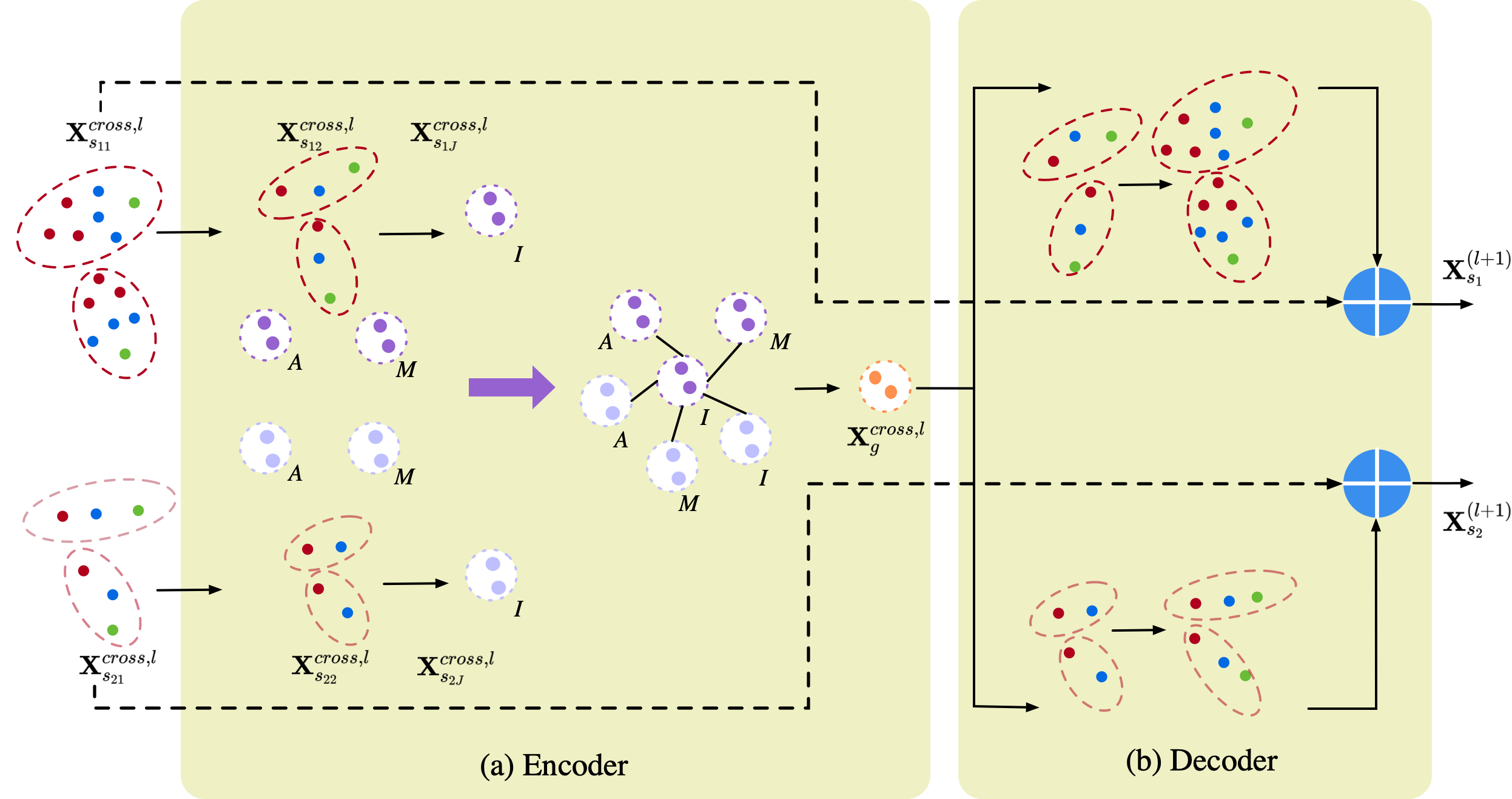
Figure 3: Architecture of the Interaction-Aware Transformer (IAT). (a) The inputs of the encoder are node-level representations from the CS-NLI module, i.e., the first subgraph in the encoder. For clear illustration, we draw several circles with different colors to show the dynamic process of graph-level representation learning. (b) The outputs of the decoder are the node-level representations from two skeletons.

III-B1 Encoder

As aforementioned in Section I, significant interaction information of mice may be lost if we adopt the pooling operation such as the global average pooling to produce graph-level representation. Hence, to learn a discriminative graph-level representation, we design a novel Interaction-Aware Transformer based on the self-attention mechanism [31, 36]. Given the node-level representation of skeleton graph $s_{i}$ on the $l$-th layer (i.e., $\mathbf{X}_{s_{i}}^{cross,l}\in\mathbb{R}^{N_{s_{i}}\times{C}_{l}\cdot{T}_{l}}$), we sequentially generate $J$ subgraphs, i.e., $\mathbf{X}_{s_{ij}}^{cross,l}\in\mathbb{R}^{N_{s_{i}}^{j}\times{C}_{l}\cdot{T}_{l}}$, with $N_{s_{i}}^{j},\forall j\in\left\{1,2,\dots,J\right\}$ nodes. Inspired by the universal transformer model [36], we design an interaction-aware self-attention mechanism using a self-attention block, followed by a recurrent transition for hierarchical spatio-temporal representation learning. Regarding node $v_{m_{j}}\in\mathcal{N}_{s_{i}}^{j}=\left\{1,2,\dots,N_{s_{i}}^{j}\right\}$ in the $j$-th subgraph (the first subgraph represents the node-level representation generated by the CS-NLI module), we have:

$$\small\begin{split}\begin{aligned} \mathbf{H}_{s_{ij+1},m_{j+1}}^{cross,l}=LN(\mathbf{Q}_{s_{ij+1},m_{j+1}}^{l}+\mathbf{\Upsilon}_{m_{j+1}}(\mathbf{X}_{s_{ij},m_{j}}^{cross,l}))\end{aligned}\end{split}$$ (13)

$$\small\begin{split}\begin{aligned} \mathbf{X}_{s_{ij+1},m_{j+1}}^{cross,l}=LN(\mathbf{H}_{s_{ij+1},m_{j+1}}^{cross,l}+\mathbf{\Gamma}(\mathbf{H}_{s_{ij+1},m_{j+1}}^{cross,l}))\end{aligned}\end{split}$$ (14)

where $LN(\cdot)$ is to normalise the inputs across the entire feature dimensions. The transition function shown in Eq. (14) is defined as a TCN that models the temporal relations between nodes. $\mathbf{\Upsilon}(\cdot)$ denotes the self-attention network to dynamically learn the graph-level representation, which can be formulated as:

$$\begin{split}\begin{aligned} \mathbf{\Upsilon}_{m_{j+1}}(\mathbf{X}_{s_{ij+1},m_{j}}^{cross,l})=\sum_{m_{j}\in\mathcal{N}_{s_{i}}^{j}}\alpha_{m_{j+1},m_{j}}^{l}\mathbf{V}_{s_{ij},m_{j}}^{l}\end{aligned}\end{split}$$ (15)

where $\alpha_{m_{j+1},m_{j}}^{l}$ represents the strength of the correlations between nodes $v_{m_{j+1}}$ and $v_{m_{j}}$, based on the query and key vectors. $\mathbf{V}_{s_{ij},m_{j}}^{l}$ is the value vector of $m_{j}$, and the score $\alpha_{m_{j+1},m_{j}}^{l}$ is used to weight each node’s key vector.

The query, key and value vectors in the Transformer architecture are used to establish a self-attention mechanism [31]. Different from most self-attention methods of applying linear transformations [36, 37] or convolution [27] to the node features, we propose an interaction-aware self-attention approach to construct the vectors, based on the structural intra- and inter-skeleton interactions. Particularly, we focus on the behaviour-related interaction saliency by condensing $N_{s_{i}}^{j}$ nodes into a sub-graph with $N_{s_{i}}^{j+1}$ nodes. Hence, the query vector is defined as:

$$\begin{split}\begin{aligned} \mathbf{Q}_{s_{ij},m_{j+1}}^{l}=\sum_{m_{j}\in N_{s_{i}}^{j}}\mathbf{W}_{s_{ij}}^{l}(m_{j+1},m_{j})\mathbf{X}_{s_{ij},m_{j}}^{cross,l}\end{aligned}\end{split}$$ (16)

where $\mathbf{W}_{s_{ij}}^{l}(m_{j+1},m_{j})$ are the elements of a trainable matrix $\mathbf{W}_{s_{ij}}^{l}\in\mathbb{R}^{N_{s_{i}}^{j+1}\times N_{s_{i}}^{j}}$ at the $m_{j+1}$-th row and $m_{j}$-th column. The output $\mathbf{Q}_{s_{ij},m_{j+1}}^{l}$ denotes the feature vector of node $v_{m_{j+1}}$. We next compute the key and value vectors for node $v_{m_{j}}$, which are jointly encoded by different interaction patterns, i.e., intra- and inter-skeleton interactions. The key vector $\mathbf{K}_{s_{ij},m_{j}}^{l}$ can be computed as follows:

$$\begin{split}\begin{aligned} \mathbf{K}_{s_{ij},m_{j}}^{l}=Conv_{1\times 1}\Big{(}[\Phi(\mathbf{X}_{s_{ij},m_{j}}^{cross,l});\Psi(\mathbf{X}_{s_{ij},m_{j}}^{cross,l})]\Big{)}\end{aligned}\end{split}$$ (17)

where $\Phi(\mathbf{X}_{s_{ij},m_{j}}^{cross,l})$ representing the intra-skeleton interaction on the spatial domain for node $v_{m_{j}}$ can be formed using Eq. (1). $\Psi(\mathbf{X}_{s_{ij},m_{j}}^{cross,l})$ denotes the corresponding inter-skeleton interaction that is calculated by combining Eqs. (9) and (10). The concatenation is performed on the channel dimension, and $Conv_{1\times 1}(\cdot)$ denotes $1\times 1$ convolution to reduce the channel dimension.

Similarly, we formulate the value vector $\mathbf{V}_{s_{ij},m_{j}}^{l}$ in Eq. (15) according to Eq. (17). Then, the attention weight $\alpha_{m_{j+1},m_{j}}^{l}$ can be defined by applying the $Softmax$ function to the scaled dot products [31] between $m_{j+1}$ and $m_{j}$:

$$\begin{split}\begin{aligned} \alpha_{m_{j+1},m_{j}}^{l}=Softmax_{m_{j}}(\frac{\mathbf{Q}_{s_{ij+1},m_{j+1}}^{l}(\mathbf{K}_{s_{ij},m_{j}}^{l})\top}{\sqrt{C_{l}T_{l}}})\end{aligned}\end{split}$$ (18)

To this end, we can hierarchically generate multiple subgraphs through Eqs. (13) and (14), in which the final one, i.e., $\mathbf{X}_{s_{iJ},m_{J}}^{cross,l}$ denotes the behaviour-related graph-level representation with $N_{s_{i}}^{J}=1$.

To generate a graph-level behavioural representation from the skeleton graph, GAP [20] or max pooling [22] has been used to merge the information of all the keypoints or frames. Intuitively, different graph-level representations carry different semantic information describing social interactions. Thus, we also explore the relations between different graph-level representations to enhance the discrimination of social behaviour.

Given the representation of the first subgraph on the $l$-th layer of our network, i.e., $\mathbf{X}_{s_{i1}}^{cross,l}$, we first calculate the average and maximum values of the representation in the spatial domain by spatial average pooling [20] $SAP(\cdot)$ (see Algorithm S1) and max pooling [22] $SMP(\cdot)$, respectively. Eqs. (13) and (14) can be treated as the implementation of function $IAT(\cdot)$ that describes the graph-level representation. Instead of fusing different graph-level representations across skeletons by direct summing over the spatial dimension, we attempt to model the relations between them using our proposed interaction-aware self-attention module to adaptively enhance the graph-level representation, formulated as follows:

$$\begin{split}\begin{aligned} \widetilde{\mathbf{X}}_{g}^{cross,l}=&IAT(\mathbf{Z}_{s_{i1}}^{cross,l})\in\mathbb{R}^{{C}_{l}\cdot{T}_{l}}\\ \mathbf{Z}_{s_{i1}}^{cross,l}=&[SAP(\mathbf{X}_{s_{11}}^{cross,l});SMP(\mathbf{X}_{s_{11}}^{cross,l});\\ &\cdots;IAT(\mathbf{X}_{s_{21}}^{cross,l})]\in\mathbb{R}^{6\times{C}_{l}\cdot{T}_{l}}\end{aligned}\end{split}$$ (19)

where $\widetilde{\mathbf{X}}_{g}^{cross,l}$ is the enhanced graph-level representation that fuses various semantic information. $\mathbf{Z}_{s_{i1}}^{cross,l}$ is the fused representation, including 3 types of graph-level representation at each skeleton branch.

III-B2 Decoder

In most existing work [25, 20], the node-level representation of one GCN-TCN block is directly fed into the next block for deeper spatio-temporal representation encoding, where the graph-level representation can be generated based on the last node-level representation. Different from these standard work, we also add a decoder to the end of the encoder to adaptively update the node-level representation before sending the representation to the next layer. We directly infer the node-level representation from the graph-level representation using our proposed interaction-aware self-attention presented in Section III-B1:

$$\begin{split}\begin{aligned} \widetilde{\mathbf{X}}_{s_{iJ}}^{cross,l}=&IAT(IAT(\mathbf{Z}_{s_{i1}}^{cross,l}))\in\mathbb{R}^{N_{s_{i}}\times{C}_{l}\cdot{T}_{l}}\end{aligned}\end{split}$$ (20)

where we define $J$ subgraphs for the decoder and the last one is $\widetilde{\mathbf{X}}_{s_{iJ}}^{cross,l}$. Hence, the node-level representation for the $(l+1)$-th layer can be updated by $\mathbf{X}_{s_{i}}^{(l+1)}=\widetilde{\mathbf{X}}_{s_{iJ}}^{cross,l}+\mathbf{X}_{s_{i}}^{cross,l}$. Our proposed IAT is summarised in Algorithm S1.

III-C Self-supervision for Cross-Skeleton Node Similarity Learning

Self-supervised learning has been applied to image [38], video [39] and graph [40] domains by generating necessary supervisory signals (i.e., pseudo labels) which are derived from data itself. In this work, there potentially exists important similarity between the two skeletons (dense and sparse skeletons) that describe the spatial structure of the mouse from different scales. In other words, the similarity are naturally embedded into the node-level representations of the two skeletons, which may play a crucial role in social behaviour representation learning. Inspired by the attribute based self-supervision [40] on graphs, we design an auxiliary self-supervised learning task to better preserve these attributes between the cross-skeleton pairwise nodes.

For the $i$-th sliding window, given the initial spatial-temporal feature of the node $v_{m}$ in skeleton $s_{1}$ (i.e., $\mathbf{X}_{s_{1},m}^{(i)}$) and that of $v_{n}$ in skeleton $s_{2}$ (i.e., $\mathbf{X}_{s_{2},n}^{(i)}$), we first compute the node feature similarity between them according to the cosine similarity:

$$\begin{split}\begin{aligned} S_{mn}^{(i)}=\frac{\mathbf{X}_{s_{1},m}^{(i)}\cdot\mathbf{X}_{s_{2},n}^{(i)}}{max\left(\left\|\mathbf{X}_{s_{1},m}^{(i)}\right\|_{2}\cdot\left\|\mathbf{X}_{s_{2},n}^{(i)}\right\|_{2},\epsilon\right)}\end{aligned}\end{split}$$ (21)

where $\epsilon$ is a small constant avoiding divide-by-zero. Then, the self-supervised learning task can be formulated as a regression problem and the corresponding loss can be defined as:

$$\begin{split}\begin{aligned} \mathcal{L}_{self}=&\frac{1}{B}\sum_{i=1}^{B}\bigg{(}\frac{1}{|\mathcal{P}|}\sum_{\left(v_{m},v_{n}\right)\in\mathcal{P}}\\ &\left\|f_{s}\left(\mathbf{X}_{s_{1},m}^{(i),l}-\mathbf{X}_{s_{2},n}^{(i),l}\right)-\mathbf{S}_{mn}^{(i)}\right\|^{2}\bigg{)}\end{aligned}\end{split}$$ (22)

where $\mathcal{P}$ denotes the set of node pairs consisting of nodes from different skeletons, and $|\mathcal{P}|$ is the number of the nodes. $f_{s}(\cdot)$ is a fully connected layer with the output dimension of 1. $\mathbf{X}_{s_{1},m}^{(i),l}$ is the node-level representation of node $v_{m}$ in the $l$-th layer of our network.

We can obtain the overall behaviour recognition loss by combining the self-supervised loss defined in Eq. (22) and cross-entropy loss defined in Eq. (23), which is defined as $\mathcal{L}=\mathcal{L}_{\text{class }}+\lambda\mathcal{L}_{\text{self }}$, where $\lambda$ is a hyper-parameter adjusting the contribution of the self-supervised loss.

$$\begin{split}\begin{aligned} \widetilde{\mathbf{Y}}&=Softmax(f_{o}(\widetilde{\mathbf{X}}_{g}^{cross}))\\ \mathcal{L}_{class}&=-\frac{1}{B}\sum_{i=1}^{B}\sum_{j=1}^{C}\mathbf{Y}_{j}^{(i)}\log\widetilde{\mathbf{Y}}_{j}^{(i)}\end{aligned}\end{split}$$ (23)

where $f_{o}(\cdot)$ is a fully connected layer. $\widetilde{\mathbf{X}}_{g}^{cross}$ represents the final representation for classification, which is constructed by concatenating the graph-level representations of different layers. $\widetilde{\mathbf{Y}}_{j}^{(i)}$ represents the predicted probability that the spatio-temporal skeleton graph with feature $\mathbf{X}^{(i)}$ belongs to class $j$, and $\mathbf{Y}_{j}^{(i)}$ is the corresponding ground truth. $B$ and $C$ denote the numbers of sliding windows and classes, respectively. By jointly optimising the self-supervised objective function and the traditional classification loss function, our proposed model can lead to more discriminative representation.

IV Experiments

IV-A Datasets and Experimental Setup

IV-A1 CRIM13-Skeleton Dataset

In this paper, we validate the proposed framework using videos of two mice. The Caltech Resident-Intruder Mouse dataset [41] (CRIM13) consists of 237x2 videos of two mice (see Table S1 for the description of social behaviour), which was used to study neurophysiological mechanisms involved in aggression and courtship in mice. It was recorded with synchronized top- and side-view cameras with the resolution of 640*480 pixels and the frame rate of 25Hz. Each video lasts about 10 minutes and was annotated frame by frame. 13 social behaviours was defined in this dataset, including 12 specific behaviors (shown in Table S1) and one otherwise unspecified behaviour (i.e., other). In this paper, we use the public CRIM13 dataset with pose annotations (CRIM13-Skeleton) in [13]. It contains 64 top-view videos where each frame has 16 keypoints (each mouse has 8 keypoints), as shown in Fig. 4(a) and S1(a). For each keypoint, it is represented by a tuple of $(X,Y,C)$, in which $(X,Y)$ is the 2D coordinates and $C$ denotes the confidence score. In our experiments, we only use 7 kypoints (0-6 in Fig. 4(a)) of each mouse due to low confidence on the tail end. Different from the original dataset [41], CRIM13-Skeleton dataset is categorised into 12 behaviours where the behaviour ’human’ is deleted. In our experiments, we randomly split the dataset into a training set of 51 videos and a test set of 13 videos.

TABLE I: Ablation experiments for the Cross-Skeleton Node-level Interaction (CS-NLI) module on the CRIM13-Skeleton dataset. We present the classification accuracy ($\%$) of each behaviour and the average accuracy over all the behaviours. The best performance is highlighted in bold.

Methods	Approach	Attack	Copulation	Chase	Circle	Drink	Eat	Clean	Sniff	Up	Walk away	Other	Average
Baseline	46.70	79.41	69.32	22.09	57.92	77.02	53.02	77.17	69.68	71.87	47.59	73.79	62.13
with dense geometric distance information
CS-NLI(w/o inter-skeleton)	58.96	75.50	71.65	32.43	56.29	74.91	60.72	85.92	64.54	77.74	49.41	63.35	64.29
CS-NLI(w inter-skeleton)	66.37	71.17	72.16	53.51	64.28	81.40	63.16	76.90	68.93	83.47	56.16	53.33	67.57
with dense velocity information
CS-NLI(w/o inter-skeleton)	56.60	78.05	71.53	31.89	55.97	78.07	55.09	74.68	67.80	79.16	50.47	62.57	63.49
CS-NLI(w inter-skeleton)	63.47	76.39	74.98	34.19	67.99	79.65	55.40	82.27	70.39	74.54	66.46	41.52	65.60
with dense geometric distance and velocity information
CS-NLI(w/o inter-skeleton)	62.04	78.01	75.55	36.89	59.75	77.54	65.87	80.55	66.51	80.71	45.40	56.67	65.46
CS-NLI(w inter-skeleton)	69.24	81.81	78.91	44.73	66.23	79.12	57.70	86.87	65.72	85.12	59.10	45.02	68.30

IV-A2 PDMB-Skeleton Dataset

Our PDMB dataset was collected in collaboration with the biologists of Queen’s University Belfast of United Kingdom, for a study on motion recordings of mice with Parkinson’s disease (PD) [6]. The neurotoxin 1-methyl-4-phenyl-1,2,3,6-tetrahydropyridine (MPTP) is used as a model of PD, which has become an invaluable aid to produce experimental parkinsonism since its discovery in 1983 [42]. All experimental procedures were performed in accordance with the Guidance on the Operation of the Animals (Scientific Procedures) Act, 1986 (UK) and approved by the Queen’s University Belfast Animal Welfare and Ethical Review Body. This dataset consists of 12*3 annotated videos (6 videos for MPTP treated mice and 6 videos for control mice) recorded by using three synchronised Sony Action cameras (HDR-AS15) (one top-view and two side-view) with frame rate of 30 fps and 640*480 resolution. All videos contain 9 behaviours of two freely behaving mice and each video lasts around 10 minutes.

The PDMB dataset [6] provides only raw videos without keypoint annotations. To obtain the location of each mouse keypoint, we also use the standard pose estimator, i.e., DeepLabCut [9], to generate the locations and confidence scores of 7 defined keypoints on every frame of 12 top-view videos. Fig. 4(b) and S1(b) show the keypoint locations in the PDMB-Skeleton dataset.

Figure 4: Keypoint labels of (a) CRIM13-Skeleton and (b) PDMB-Skeleton datasets. The CRIM13-Skeleton dataset contains 8 keypoints for each mouse (i.e., 0-left ear, 1-right ear, 2-snout, 3-centroid, 4-left lateral, 5-right lateral, 6-tail base and 7-tail end). The PDMB-Skeleton dataset contains 7 keypoints for each mouse (i.e., 0-left ear, 1-right ear, 2-snout, 3-centroid, 4-left hip, 5-right hip and 6-tail base).

IV-A3 Implementation Details

All the experiments are performed with PyTorch 1.4.0 on a server with an Intel Xeon CPU @ 2.40GHz and two 16GB Nvidia Tesla P100 GPUs. The parameters are optimised by the Adam algorithm. For the two datasets, we use the initial learning rate of 1e-4 and all the keypoint locations are normalised before training. No data augmentation is used for fair performance comparison. $\beta$ and batch size $B_{b}$ are set to 0.5 and 128, respectively. As far as it concerns the model architecture, we use 3 cascaded CS-NLI+IAT modules, whose feature dimensions are 64, 128 and 256, respectively. The source code will be available at: https://github.com/FeixiangZhou/CS-IGANet.

IV-B Ablation Study

In this section, we launch comprehensive experiments to investigate the effectiveness of each model component, i.e., Cross-Skeleton Node-level Interaction, Interaction-Aware Transformer, Self-supervision for cross-skeleton node similarity learning in our proposed CS-IGANet. We conduct ablation experiments on the CRIM13-Skeleton and PDMB-Skeleton datasets and use a 3-layer single-stream (keypoint) GCN-TCN network [20] as our baseline model, where feature dimensions are 64, 128 and 256, respectively. Normally, classification accuracy is defined as the percentage of the samples that are correctly classified against the number of the overall samples. While it is a valid measure, this metric cannot disclose the characteristics of the datasets that have a severe imbalanced classification problem. Following [6], we here employ the averaging recognition rate per behaviour to better measure the system performance.

Figure 5: Visualisation of the learned topologies of a social behaviour sample ’approach’ on the CRIM13-Skeleton dataset. (a) The topologies representing intra-skeleton interactions of mice $k_{1}$ (top) and $k_{2}$ (bottom). The number of keypoint $V$ is 7 and its configuration is shown in Fig. S1. Here, we show the summation of the learned topologies on the three subsets generated by the partition strategy [25]. (b) The topologies of bidirectional inter-skeleton interactions learned by our model, i.e., $\mathbf{A}_{k_{1}\to k_{2}}^{l=1}$ (top) and $\mathbf{A}_{k_{2}\to k_{1}}^{l=1}$ (bottom). (c) The topologies of cross-skeleton interactions ($s_{1}$ to $s_{2}$) learned by our model, i.e., $\mathbf{A}_{s_{1}\to s_{2}}^{l=1}$ (top) and $\widetilde{\mathbf{A}}_{s_{1}\to s_{2}}^{l=1}$ (bottom). For each category, we use red lines to highlight the interactions with high significance. Zoom in for the best visualisation.

TABLE II: Ablation experiments for the Interaction-aware Transformer (IAT) on the CRIM13-Skeleton dataset.

Methods	Approach	Attack	Copulation	Chase	Circle	Drink	Eat	Clean	Sniff	Up	Walk away	Other	Average
Baseline	46.70	79.41	69.32	22.09	57.92	77.02	53.02	77.17	69.68	71.87	47.59	73.79	62.13
IAT(I $\&$ w/o DC)	59.22	78.07	66.23	42.84	62.83	80.53	59.35	88.07	66.85	82.92	52.79	47.60	65.61
IAT(I $\&$ w DC)	62.53	80.37	70.80	35.41	65.97	80.70	64.50	85.47	64.48	81.92	61.49	49.09	66.89
IAT(I+M $\&$ w DC)	65.53	78.46	71.43	51.62	57.99	81.05	56.74	88.46	67.10	81.94	60.13	44.30	67.06
IAT(I+A $\&$ w DC)	63.80	74.20	77.02	50.95	63.27	82.46	60.45	83.43	65.53	83.72	60.23	48.21	67.77
IAT(I+A+M $\&$ w DC)	61.96	77.05	72.98	52.84	62.52	81.58	59.90	81.99	71.63	81.34	60.60	49.92	67.85
IAT($G$(I,A,M) $\&$ w DC)	63.20	75.90	73.83	55.0	75.91	79.65	67.29	83.95	67.21	84.46	60.60	41.03	69.0

Figure 6: Learned topologies (i.e., inter-skeleton interaction $\mathbf{A}_{k_{1}\to k_{2}}^{l=1}$ ) by our CS-NLI module for three sample social behaviours (e.g., approach, chase and walk away) (a) and the motion trajectories for three behaviours in the CRIM13-Skeleton dataset (b). For each behaviour shown in (a), each topology refers to the social interaction between mice in the current frame. The corresponding motion trajectories of keypoints is shown in (b). In (b), blue and red points indicate the keypoints of the resident mouse and the intruder, respectively. Blue and red arrows represent the direction of motion. More examples of motion trajectories can be found in Fig. S4. Best viewed in color.

IV-B1 Effects of Cross-Skeleton Node-level Interaction

Here, we investigate the influences of the proposed Cross-Skeleton Node-level Interaction module. We study the effects of dense geometric distance in Eq. (2), dense velocity in Eq. (3) as well as inter-skeleton interaction (denoted as inter-skeleton) block, presented in Table I. We observe that the baseline method achieves relatively low accuracy for behaviours such as ’approach’, ’chase’ and ’walk away’. The low accuracy is due to the fact it only focuses on intra-skeleton interaction without considering the social interaction between mice. In addition, directly modelling cross-skeleton interaction of the same mouse based on dense geometric distance or velocity information, without inter-skeleton interaction and cross-skeleton interaction of different mice, can help slightly improve the average accuracy. The performance can be further improved to 65.46$\%$ by fusing the two types of information, confirming that the dense geometric distance and velocity information are beneficial to cross-skeleton interaction encoding. With respect to the inter-skeleton interaction modelling, we witness that the models with inter-skeleton interaction based on different types of information achieve better performance than the models without such interaction. In particular, for social behaviours such as ’approach’, ’chase’ and ’walk away’, we can obtain 7.2$\%$, 7.84$\%$ and 13.7$\%$ improvements, respectively by modelling inter-skeleton interaction (see the last two rows). Such significant improvements are due to the social interaction encoded by our CS-NLI module effectively. By jointly modelling intra-, inter- and cross-skeleton interactions based on multi-order dense information, our method achieves the best average accuracy of 68.3$\%$, which is a 6.17$\%$ improvement against the baseline model.

TABLE III: Ablation experiments for the self-supervision of Cross-Skeleton Node Similarity Learning on the CRIM13-Skeleton dataset.

Methods	Approach	Attack	Copulation	Chase	Circle	Drink	Eat	Clean	Sniff	Up	Walk away	Other	Average
CS-NLI(w/o self, $\lambda=0$)	69.24	81.81	78.91	44.73	66.23	79.12	57.70	86.87	65.72	85.12	59.10	45.02	68.30
CS-NLI(w self, $\lambda=0.1$)	59.65	79.62	74.83	57.16	64.91	80.87	64.19	82.86	63.45	83.07	75.32	49.79	69.65
CS-NLI(w self, $\lambda=0.5$)	62.40	77.69	74.55	61.62	79.43	83.33	65.60	85.17	63.40	87.07	63.94	42.76	70.58
CS-NLI(w self, $\lambda=1$)	67.50	81.43	65.73	48.66	77.04	82.81	64.09	84.96	66.72	89.04	59.44	45.25	69.39
CS-NLI(w self, $\lambda=1.5$)	59.68	76.45	80.03	47.43	77.61	83.33	55.15	80.52	61.75	86.90	66.24	52.51	68.97

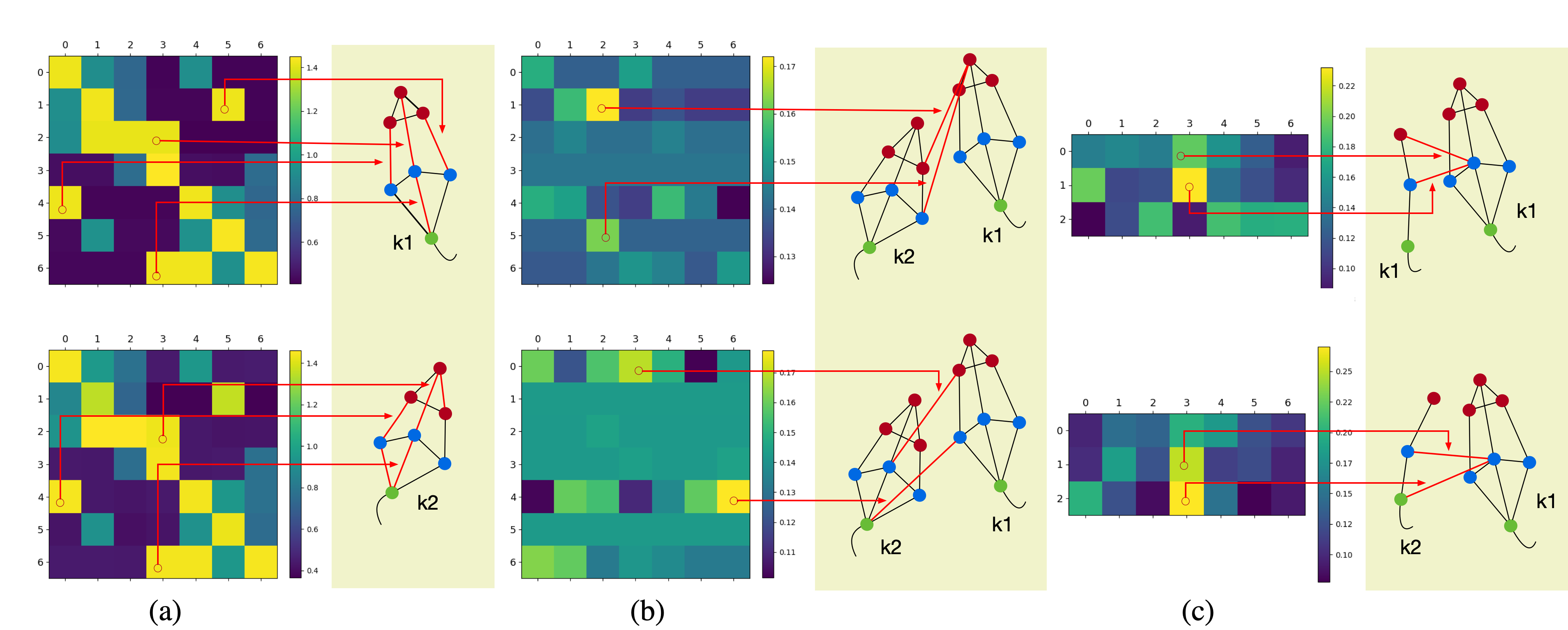
Figure S2: Visualisation of the learned topologies of a social behaviour sample ’approach’ on the CRIM13-Skeleton dataset (at the beginning of training, i.e., epoch=10). (a) The topologies representing intra-skeleton interactions of mouse $k_{1}$ (top) and $k_{2}$ (bottom). The number of keypoints V is 7 and its configuration is shown in Fig. S1. Here, we show the summation of the learned topologies on the three subsets generated by the partition strategy [25]. (b) The topologies of bidirectional inter-skeleton interactions learned by our model, i.e., $\mathbf{A}_{k_{1}\to k_{2}}^{l=1}$ (top) and $\mathbf{A}_{k_{2}\to k_{1}}^{l=1}$ (bottom). (c) The topologies of cross-skeleton interactions ($s_{1}$ to $s_{2}$) learned by our model, i.e., $\mathbf{A}_{s_{1}\to s_{2}}^{l=1}$ (top) and $\widetilde{\mathbf{A}}_{s_{1}\to s_{2}}^{l=1}$ (bottom). For each type, we use red lines to indicate the interactions with high significance. We observe that the module generates relatively dense fully connected graph at the beginning of training, especially for the inter- and -cross interactions, i.e., interactions not related to behaviours. On the contrary, our final module (Fig. 5) tends to give less attention to trivial interactions.

We also visualise the relevant interaction patterns identified by our CS-NLI module, including the intra-, inter-, and cross-skeleton interactions. Fig. 5 shows the corresponding topologies of a behaviour sample ’approach’ in the top branch of Fig. 2 (i.e., skeleton $s_{1}$ to skeleton $s_{2}$). The values close to 0 indicate weak relationships between keypoints and vice versa. From Fig. 5(a), we observe that the two topologies representing the intra-skeleton interactions of mice are very similar, where the correlations between some keypoint pairs are relatively strong, e.g. the correlation between the centroid and the tail base, and the correlation between the left lateral and the tail base. However, these independent relationships derived from each mouse are insufficient to be exploited to encode complex social interactions. The inter-skeleton interaction modelling is able to learn new interactions between mice where the independent skeleton graph cannot provide, as shown in Fig. 5(b). For instance, our CS-NLI module pays much attention to the interactions between the tail bases of mice, and between the left ear and the snout when considering the effect of mice $k_{2}$ on $k_{1}$. Moreover, in Fig. 5(c), our CS-NLI module further models the cross-skeleton interactions, where the tail bases of the same mice or different mice from different scales are highly related. To examine the difference of the topologies during training, we also show topologies learned by our CS-NLI module that is not be fully trained, as shown in Fig. S2. We observe that the model generates a relatively dense fully connected graph at the beginning of training, especially for the inter- and -cross interactions, where interactions may not be related to behaviours. On the contrary, our final model tends to better focus on behaviour related interactions. To show how our CS-NLI module works, we display the learned topologies representing the inter-skeleton interaction, i.e., $\mathbf{A}_{k_{1}\to k_{2}}^{l=1}$, in Fig. 6. From this figure, we observe that the CS-NLI module gives much attention to the interactions between mice, e.g., left lateral and left ear for ’approach’, tail base and left ear for ’chase’, and tail bases for ’walk away’.

IV-B2 Effects of Interaction-aware Transformer

In order to validate the effectiveness of our proposed IAT module, we design six structures using the baseline model. IAT (I $\&$ w/o DC) refers to the case where we only keep the encoder of the IAT and use the graph-level representation aggregated by $IAT(\cdot)$ ($I$) to perform behavioural classification, while IAT (I $\&$ w DC) refers to a structure with the encoder and the decoder. IAT (I+M $\&$ w DC) and IAT (I+A $\&$ w DC) means that we enhance the graph-level representation by combining graph-level representation from the encoder and that generated by spatial max pooling and average pooling, respectively, where we simply use the sum operation to fuse different representations. The last IAT ($G$(I,A,M) $\&$ w DC) refers to the structure that models the interactions between multi-level graph representations. From Table II, we observe that the IAT without any decoder achieves higher accuracy than the baseline model for all 8 behaviours, indicating that the intra-skeleton interaction of each mouse and inter-skeleton interactions between mice are important to graph-level representation learning. The performance is further improved by constructing an encoder-decoder framework, resulting in the highest accuracy of 80.37$\%$ and 61.49$\%$ for ’attack’ and ’walk away’, respectively. This is because the node-level representation can be adaptively updated by our proposed dual-path decoder, before it is fed into the next layer, which helps to identify higher-level features. In addition, three models combining different graph-level representations through the simple sum operation all outperform IAT (I $\&$ w DC), suggesting that different graph-level representations carry complementary spatio-temporal information that helps improve the identification. Instead of fusing different graph-level representations by the sum operation, we explore the structural relations by our proposed interaction-aware self-attention unit, leading to a 1.15$\%$ improvement against IAT (I+A+M $\&$ w DC). Regarding our network involving two skeletons, we fuse different graph-level representations from two skeleton branches by the interaction-aware self-attention module.

IV-B3 Effects of Self-supervision for Cross-Skeleton Node Similarity Learning

In this subsection, we study the effect of the proposed auxiliary self-supervised loss function, controlled by the hyper-parameter $\lambda$. To analyse the impact of this parameter, we train several models (i.e., CS-NLI module) with different values of $\lambda$. As shown in Table III, all models with self-supervision ($\lambda=0.1,0.5,1,1.5$) lead to an improvement over the baseline without self-supervision. Increasing $\lambda$ from 0 to 0.5 significantly improves the accuracy. This is mainly because the important attributes (i.e., similarity) underlying cross-skeleton pairwise nodes are explicitly exploited in the node representation learning. When $\lambda=0.5$, we achieve significant improvements on the accuracy of ’chase’, ’circle’, ’drink’ and ’eat’, and the highest average accuracy of 70.58$\%$. However, there is significant degradation in the performance when we increase $\lambda$ to 1.5. This drop is due to the fact that the self-supervised loss severely penalises the inherent attributes of node pairs from different skeletons. Hence, our default value is $\lambda=0.5$.

TABLE IV: Ablation experiments for the CS-NLI, IAT and self-supervision modules on the CRIM13-Skeleton and PDMB-Skelton datasets.

Dataset	CS-NLI	IAT	Self-supervision	Average
CRIM13-Skeleton				62.13
	$\surd$			68.30
		$\surd$		69.0
	$\surd$		$\surd$	70.58
	$\surd$	$\surd$	$\surd$	73.75
PDMB-Skeleton				52.67
	$\surd$			59.24
		$\surd$		60.03
	$\surd$		$\surd$	60.59
	$\surd$	$\surd$	$\surd$	62.33

Figure 7: t-SNE visualization of the features learned by (a) 2s-AGCN, (b) MS-G3D, (c) MV-IGNet, (d) Our method. Each point represents a skeleton sequence. We show 11 behaviour classes of the CRIM13-Skeleton dataset, indicated by colors.

We also investigate the contribution of the proposed CS-NLI, IAT and Self-supervision modules to the whole network on both datasets. In addition to adding each proposed module to the baseline model separately, we further employ the proposed modules applied to the baseline model simultaneously. The results are reported in Table IV. On the two datasets, our method achieves the highest average accuracy, 73.75$\%$ and 62.33$\%$ respectively, with the three proposed modules applied simultaneously, which are of 11.62$\%$ and 9.66$\%$ increments compared to the baseline model.

TABLE V: Classification accuracy ($\%$) comparison against state-of-the- art methods on the CRIM13-Skeleton dataset. The best performance is highlighted in bold.

Methods	Approach	Attack	Copulation	Chase	Circle	Drink	Eat	Clean	Sniff	Up	Walk away	Other	Average
ST-GCN[25]	34.34	75.68	68.97	35.56	34.65	73.33	45.87	73.53	64.31	69.75	26.27	75.80	56.51
2s-AGCN[20]	51.03	83.40	75.84	36.46	53.40	75.61	63.65	76.71	75.80	76.25	40.04	51.15	63.28
SGN[22]	49.57	80.43	74.90	34.90	66.42	75.44	63.26	83.83	66.19	75.67	41.78	57.41	64.15
PA-ResGCN[17]	57.04	74.56	77.81	22.98	51.64	80.88	55.90	82.99	75.42	85.15	40.44	69.16	64.50
MS-G3D[26]	57.38	80.08	69.79	56.61	75.28	65.79	72.74	66.00	55.96	82.00	52.03	49.29	65.24
MV-IGNet[19]	55.33	73.77	77.81	48.78	60.31	81.75	51.59	80.81	78.43	83.40	57.83	64.56	67.86
ST-TR[27]	45.92	74.86	74.93	44.93	78.43	79.12	54.49	84.84	72.85	89.19	60.69	23.04	65.27
EfficientGCN[43]	52.99	78.47	75.12	33.12	44.97	81.23	55.36	80.20	77.96	83.23	55.29	66.39	65.36
CTR-GCN[28]	52.33	79.45	75.89	41.59	53.08	66.67	55.50	68.12	73.70	78.71	48.83	60.58	62.83
Ours(CS-NLI+self)	62.40	77.69	74.55	61.62	79.43	83.33	65.60	85.17	63.40	87.07	63.94	42.76	70.58
Ours(IAT)	63.20	75.90	73.83	55.0	75.91	79.65	67.29	83.95	67.21	84.46	60.60	41.03	69.0
Ours(CS-IGANet)	67.30	84.30	75.30	69.32	82.08	81.75	63.44	88.20	73.47	87.69	66.79	45.38	73.75

TABLE VI: Classification accuracy comparison against several state-of-the- art methods on the PDMB-Skeleton dataset.

Methods	Approach	Chase	Circle	Eat	Clean	Sniff	Up	Walk away	Other	Average
ST-GCN[25]	52.72	44.24	50.62	53.24	45.84	30.61	66.74	38.09	81.69	51.53
2s-AGCN[20]	54.84	42.17	53.89	51.08	48.36	50.40	74.04	41.78	61.95	53.17
SGN[22]	53.96	41.47	47.19	56.56	46.77	44.54	73.13	40.82	76.13	53.40
PA-ResGCN[17]	59.06	45.16	52.34	58.99	50.98	43.11	67.71	50.35	78.84	56.28
MS-G3D[26]	58.10	44.01	61.99.	57.55	47.10	70.0	69.13	37.36	48.92	54.91
MV-IGNet[19]	51.47	45.39	51.40	55.40	57.22	42.28	89.45	39.15	75.17	56.33
ST-TR[27]	56.33	50.69	51.87	59.71	46.81	41.49	72.76	49.95	61.25	54.54
EfficientGCN[43]	56.28	40.09	51.56	51.80	51.28	44.77	74.18	37.91	80.25	54.23
CTR-GCN[28]	46.48	48.39	50.93	54.68	50.51	68.83	62.69	38.52	50.55	52.32
Ours(CS-NLI+self)	65.83	60.83	62.93	56.12	54.03	63.60	75.16	52.44	54.40	60.59
Ours(IAT)	61.34	60.37	56.70	58.99	53.04	68.22	74.52	50.68	56.25	60.03
Ours(CS-IGANet)	66.43	63.13	63.40	57.55	58.08	71.33	70.53	53.66	56.88	62.33

IV-C Comparison to State-of-the-Art Approaches

In this section, we compare the proposed model against several state-of-the-art graph-based methods on two datasets: CRIM13-Skeleton and PDMB-Skeleton. The results are presented in Tables V and VI, respectively. For all the existing methods, we follow their default settings in our experiments.

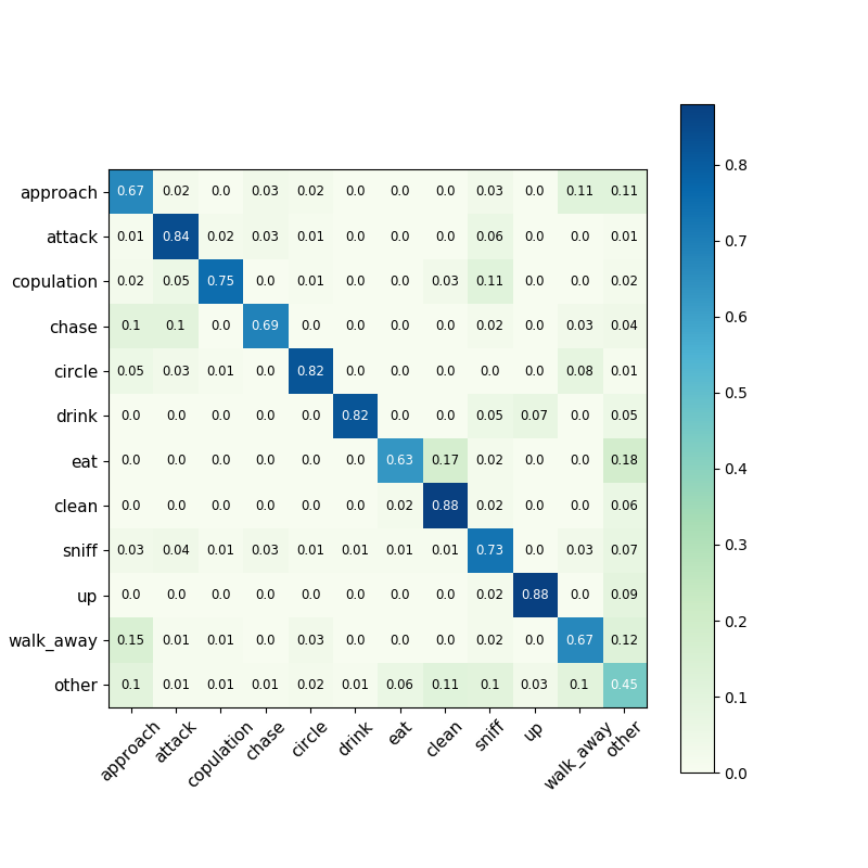
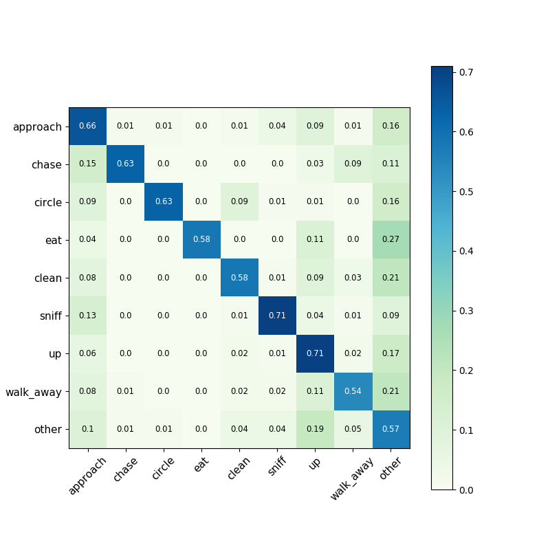
(a) CRIM13-Skeleton	(b) PDMB-Skeleton

Figure S3: Confusion matrices of our method (i.e., CS-IGANet) on CRIM13-Skeleton (a) and PDMB-Skeleton datasets (b). The diagonal cells in each confusion matrix show the percentage of correct classifications. The confusion matrix is obtained for measuring the agreement between the ground-truth (row) and the predicted labels (column). The non-diagonal cells contain the percentages of the incorrectly classified behaviors. In each row, all the values should sum to be 1. The higher probabilities along the diagonal and the lower off-diagonal values indicate the degrees of successful classification for all the categories. The colour bar indicates the degree of the agreement whilst deep blue indicates the agreements close to 100$\%$.

Looking at Table V, our proposed modules and their combination outperform the other state of the art models on the average accuracy. Notably, our method jointly models the intra-, inter- and cross-skeleton interactions, and dynamically learns graph-level representation of mouse social behaviours, which is very effective in representation learning of mouse social behaviour. Although ST-GCN [25] achieves the highest classification accuracy on ’other’, its average accuracy of all the behaviours is the lowest among these methods. This is because it only uses a fixed skeleton topology to model the relations between keypoints of each mouse, limiting its ability to encode/decode intra-skeleton interaction for some specific behaviours, such as ’eat’ and ’up’. Compared with CTR-GCN [28], our CS-IGANet outperforms the standard method by a large margin, where our average accuracy holds 10.92$\%$ improvement. This suggests that dynamic refinement of channel-wise topology is not powerful enough to maintain the quality of mouse social behaviour representation. We also notice that MV-IGNet [19] achieves the best performance among the 9 existing methods, but there is still a large gap (i.e., 5.89$\%$) between MV-IGNet and our CS-IGANet. In addition, for social interactions such as approach, chase and walk away, our proposed CS-IGANet improves the accuracy with large margins of 9.92$\%$, 12.71$\%$ and 6.1$\%$, respectively, compared with their close competitors. We also show the confusion matrix of our CS-IGANet on the CRIM13-Skeleton dataset, as shown in Fig. S3(a).

Additionally, we present in Fig. 7 the t-SNE visualisation of the representations learned by our model and other 3 state-of-the-art methods (i.e., 2s-AGCN, MS-G3D and MV-IGNet). For our model, the representation is the concatenation of graph-level outputs of different layers, i.e., $\widetilde{\mathbf{X}}_{g}^{cross}$. Our proposed CS-IGANet leads to better separation of the 11 behaviour classes. In particular, for some similar behaviours such as ’approach’ and ’walk away’, our model can better distinguish them.

As for the PDMB-Skeleton dataset, our approach also achieves the state-of-the-art performance with average accuracy of 62.33$\%$, which is a 6$\%$ improvement compared with the closest competitor, i.e., MV-IGNet. In addition, our CS-IGANet significantly outperforms the other state-of-the-art methods on behaviours ’approach’, ’chase’, ’circle’ and ’walk away’, and achieve comparable performance on ’clean’ and ’sniff’, compared to [19] and [26]. The confusion matrix of our CS-IGANet on the PDMB-Skeleton dataset is shown in Fig. S3(b).

V Conclusion

In this work, we have presented a novel architecture called Cross-Skeleton Interaction Graph Aggregation Network (CS-IGANet) for representation Learning of mouse social behaviour. Cross-Skeleton Node-level Interaction module (CS-NLI) strengthens the node-level representation of each mouse by modelling intra-, inter- and cross-skeleton interactions in an unified way. We also designed a novel Interaction-Aware Transformer (IAT) to hierarchically aggregate node-level representation into graph-level representation of social behaviour, and adaptively update the node-level representation, which is guided by our interaction-aware self-attention unit. An auxiliary self-supervised learning task was also proposed to focus on the similarity between cross-skeleton pairwise nodes, enhancing the representation ability of our model. Experimental results on CRIM13-Skeleton and PDMB-Skeleton datasets demonstrated that the proposed approach outperformed most of the baseline methods.

Supplementary A

ST-GCN [25] is the first work adopting Graph Convolutional Networks for skeleton data modelling. It is constructed by stacked spatio-temporal blocks, each of which is composed of a spatial convolution (GCN) block, followed by a temporal convolution (TCN) block. The spatial module utilizes the GCN to model the structural dependencies of nodes, which is formulated as:

$$\begin{split}\mathbf{X}_{t}^{(l+1)}=\sum_{k}^{K_{v}}\mathbf{W}_{k}\left(\mathbf{X}_{t}^{l}\mathbf{A}_{k}\right)\end{split}$$ (1)

where $K_{v}$ denotes the kernel size. $l$ is the layer index of the GCN. $\mathbf{W}_{k}$ is a trainable weight matrix that is implemented as $C_{\text{out }}\times C_{\text{in }}\times 1\times 1$ convolution operation, where $C_{\text{out }}$ and $C_{\text{in}}$ are the output and input channels. $\mathbf{A}_{k}=\mathbf{\Lambda}_{k}^{-\frac{1}{2}}\tilde{\mathbf{A}}_{k}\mathbf{\Lambda}_{k}^{-\frac{1}{2}}$, where $\tilde{\mathbf{A}}_{k}$ is the adjacency matrix of the skeleton graph indicating intra-skeleton connections. $\mathbf{\Lambda}_{k}$ is the diagonal matrix, where $\mathbf{\Lambda}_{k}^{ii}=\sum_{j}\left(\tilde{\mathbf{A}}_{k}^{ij}\right)+c$, and $c$ is a small constant avoiding empty rows. On the temporal dimension, TCN is implemented by applying a $K_{t}\times 1$ 2D convolution operation to the input $\mathbf{X}\in\mathbb{R}^{C\times T\times N}$ with $(T,N)$ dimensions, where $K_{t}$ is the kernel size.

The structure of the skeleton graph shown in Eq. (1) is predefined by a fixed adjacency matrix. In order to learn an adaptive topology, [20] presented the Adaptive Graph Convolutional Network (A-GCN), in which the adjacency matrix is divided into three complementary parts, as shown in Eq. (2):

$$\begin{split}\mathbf{X}_{t}^{(l+1)}=\sum_{k}^{K_{v}}\mathbf{W}_{k}\mathbf{X}_{t}^{l}\left(\mathbf{A}_{k}+\mathbf{B}_{k}+\mathbf{C}_{k}\right)\end{split}$$ (2)

where $\mathbf{A}_{k}$ is the same as the one shown in Eq. (1), which represents the physical structure of human body. $\mathbf{B}_{k}$ can be learned according to the training data and its elements can be an arbitrary value. It indicates the existence and strength of the connections between two nodes. $\mathbf{C}_{k}$ determines the connection strength between two nodes by calculating their similarity using the normalised embedded Gaussian function.

Algorithm S1 Interaction-aware Transformer (IAT) reasoning process.

0:  Spatial-temporal node-level representation embedded with intra-, inter- and cross-skeleton interactions, i.e., $\mathbf{X}_{s_{i}}^{cross,l}$ shown in Eq. (12).

0:  Graph-level representation $\widetilde{\mathbf{X}}_{g}^{cross}$ for social behaviour classification.

1:  for $l\leftarrow 1$ to $L$ do

2:     for $i\leftarrow 1$ to $I$ do

3:        for $j\leftarrow 1$ to $J-1$ do

4:           $\mathbf{H}_{s_{ij+1},m_{j+1}}^{cross,l}\leftarrow LN(\mathbf{Q}_{s_{ij+1},m_{j+1}}^{l}+\mathbf{\Upsilon}_{m_{j+1}}(\mathbf{X}_{s_{ij},m_{j}}^{cross,l}))$ (Eq. (13));

5:           $\mathbf{X}_{s_{ij+1},m_{j+1}}^{cross,l}\leftarrow LN(\mathbf{H}_{s_{ij+1},m_{j+1}}^{cross,l}+\mathbf{\Gamma}(\mathbf{H}_{s_{ij+1},m_{j+1}}^{cross,l}))$ (Eq. (14));

6:        end for

7:        $SAP(\mathbf{X}_{s_{i1}}^{cross,l})\leftarrow\frac{1}{N_{s_{i}}^{1}}\sum_{m_{1}=1}^{N_{s_{i}}^{1}}\mathbf{X}_{s_{i1},m_{1}}^{cross,l}$ ;

8:        $SMP(\mathbf{X}_{s_{i1}}^{cross,l})\leftarrow max_{m\in\mathcal{N}_{s_{i}}^{1}}(\mathbf{X}_{s_{i1},m_{1}}^{cross,l})$;

9:        $IAT(\mathbf{X}_{s_{i1}}^{cross,l})\leftarrow\mathbf{X}_{s_{iJ},m_{J}}^{cross,l}$ (w.r.t Eqs. (13) and (14));

10:     end for

11:     $\widetilde{\mathbf{X}}_{g}^{cross,l}\leftarrow IAT([SAP(\mathbf{X}_{s_{11}}^{cross,l});\cdots;IAT(\mathbf{X}_{s_{I1}}^{cross,l})])$ (Eq. (19));

12:     if $l<L$ then

13:        $\widetilde{\mathbf{X}}_{s_{iJ}}^{cross,l}\leftarrow IAT(\widetilde{\mathbf{X}}_{g}^{cross,l})$ (20));

14:        $\mathbf{X}_{s_{i}}^{(l+1)}=\widetilde{\mathbf{X}}_{s_{iJ}}^{cross,l}+\mathbf{X}_{s_{i}}^{cross,l}$;

15:        $\mathbf{X}_{s_{i}}^{cross,(l+1)}=CS-NLI(\mathbf{X}_{s_{i}}^{(l+1)})$ (w.r.t Eqs. (1), (10) and (12));

16:     end if

17:  end for

18:  $\widetilde{\mathbf{X}}_{g}^{cross}\leftarrow[\widetilde{\mathbf{X}}_{g}^{cross,1};\widetilde{\mathbf{X}}_{g}^{cross,2};\cdots;\widetilde{\mathbf{X}}_{g}^{cross,L}]$

19:  return  Final graph-level representation $\widetilde{\mathbf{X}}_{g}^{cross}$.

Supplementary B

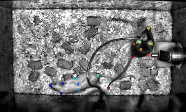
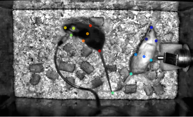
(a) CRIM13-Skeleton

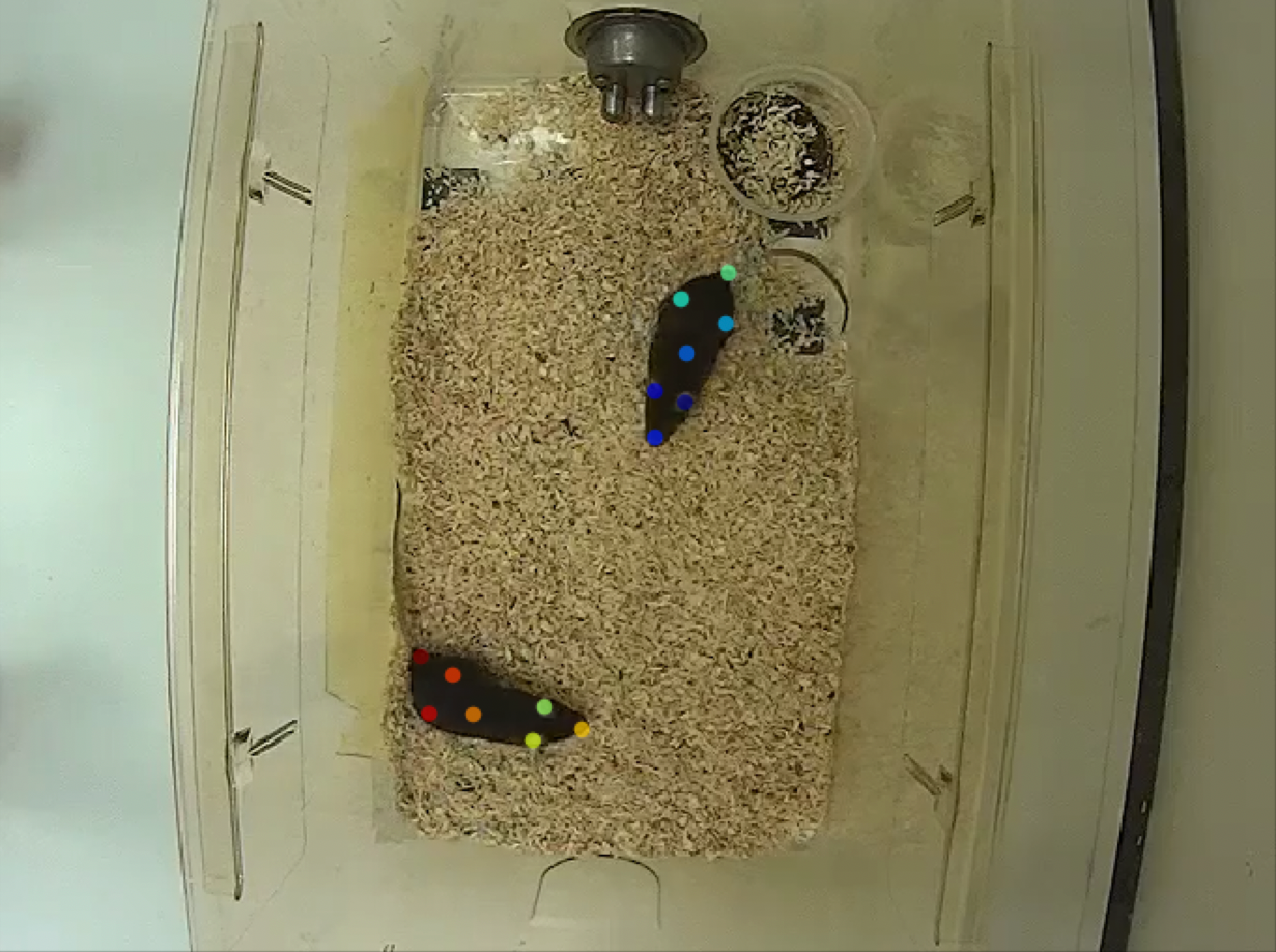
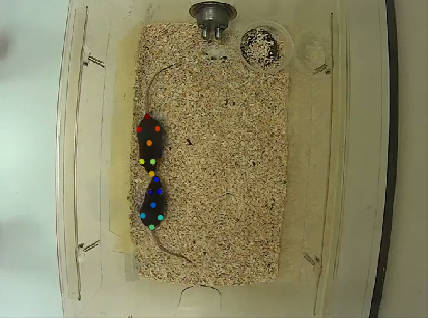
(b) PDMB-Skeleton

Figure S1: Annotated locations of different mouse keypoints on the CRIM13-Skeleton and PDMB-Skeleton datasets. (a) The public CRIM13-Skeleton dataset [13] contains 8 keypoints for each mouse (i.e., 0-left ear, 1-right ear, 2-snout, 3-centroid, 4-left lateral, 5-right lateral, 6-tail base and 7-tail end). The numbers represent the order which the body-parts were annotated. (b) To establish our PDMB-Skeleton dataset, we extract frames every 500ms for each video, and all the extracted video frames were annotated using a freeware DeepLabCut (available at https://github.com/DeepLabCut/DeepLabCut). A team of five professionals were trained to annotate the keypoints of each mouse. Similar to the CRIM13-Skeleton dataset, we annotate the locations of 7 body parts (i.e., 0-left ear, 1-right ear, 2-snout, 3-centroid, 4-left hip, 5-right hip and 6-tail base) for each mouse. We do not annotate the tail end because this keypoint is often occluded and the mouse tail is highly deformable in videos. We only use 7 body parts in all experiments on both PDMB-Skeleton and CRIM13-Skeleton datasets. In particularly, we ensure that the identity of each mouse remains unchanged during the process of annotation.

Supplementary C

TABLE S1: Ethogram of the observed behaviours, derived from CRIM13 [41]

Behaviour	Description
approach	Moving toward another mouse in a straight line without obvious exploration.
attack	Biting/pulling fur of another mouse.
copulation	Copulation of male and female mice.
chase	A following mouse attempts to maintain a close distance to another mouse while the latter is moving.
circle	Circling around own axis or chasing tail
drink	Licking at the spout of the water bottle
eat	Gnawing/eating food pellets held by the fore-paws.
clean	Washing the muzzle with fore-paws (including licking fore-paws) or grooming the fur or hind-paws by means of licking or chewing.
human	Human intervenes with mice.
sniff	Sniff any body part of another mouse.
up	Exploring while standing in an upright posture.
walk away	Moving away from another mouse in a straight line without obvious exploration.
other	ehaviour other than defined in this ethogram, or when it is not visible what behaviour the mouse displays.

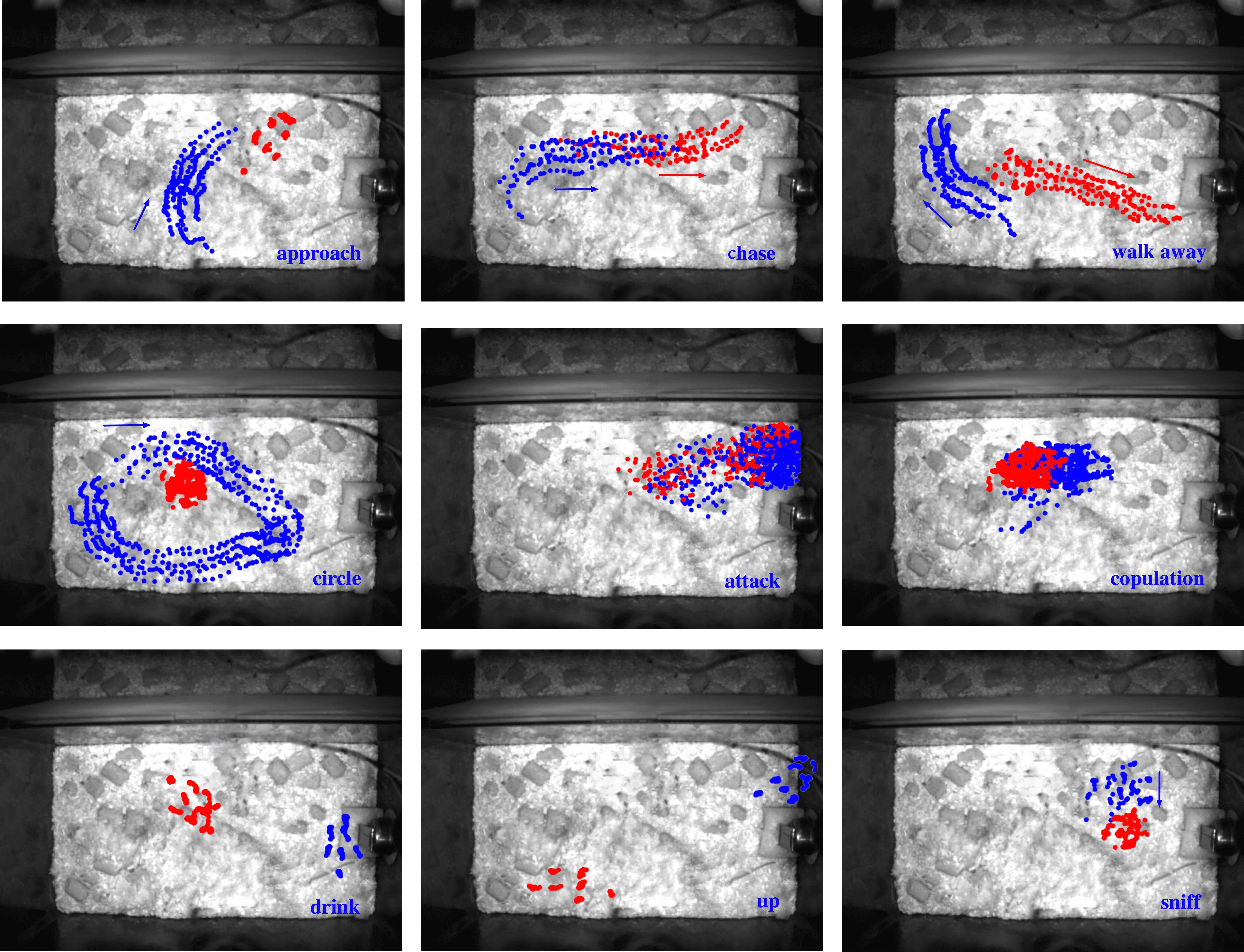
Figure S4: Examples of motion trajectory of different behaviours in the CRIM13-Skeleton dataset. Blue and red points indicate the keypoints of the resident mouse and the intruder, respectively. Blue and red arrows represent the direction of motion. For some behaviours (e.g., clean and up) without significant movement, we do not give the direction of motion.

References

- [1] Y. K. Urbach, K. A. Raber, F. Canneva, A.-C. Plank, T. Andreasson, H. Ponten, J. Kullingsjö, H. P. Nguyen, O. Riess, and S. von Hörsten, “Automated phenotyping and advanced data mining exemplified in rats transgenic for huntington’s disease,” Journal of neuroscience methods, vol. 234, pp. 38–53, 2014.
- [2] L. Lewejohann, A. M. Hoppmann, P. Kegel, M. Kritzler, A. Krüger, and N. Sachser, “Behavioral phenotyping of a murine model of Alzheimer’s disease in a seminaturalistic environment using RFID tracking,” Behavior Research Methods, vol. 41, no. 3, pp. 850–856, 2009.
- [3] C. A. Wilson and J. I. Koenig, “Social interaction and social withdrawal in rodents as readouts for investigating the negative symptoms of schizophrenia,” European Neuropsychopharmacology, vol. 24, no. 5, pp. 759–773, 2014.
- [4] S. R. Blume, D. K. Cass, and K. Y. Tseng, “Stepping test in mice: A reliable approach in determining forelimb akinesia in MPTP-induced Parkinsonism,” Experimental Neurology, vol. 219, no. 1, pp. 208–211, 2009.
- [5] Z. Jiang, D. Crookes, B. D. Green, Y. Zhao, H. Ma, L. Li, S. Zhang, D. Tao, and H. Zhou, “Context-aware mouse behavior recognition using hidden markov models,” IEEE Transactions on Image Processing, vol. 28, no. 3, pp. 1133–1148, 2018.
- [6] Z. Jiang, F. Zhou, A. Zhao, X. Li, L. Li, D. Tao, X. Li, and H. Zhou, “Muti-view mouse social behaviour recognition with deep graphic model,” IEEE Transactions on Image Processing, 2021.
- [7] A. Arac, P. Zhao, B. H. Dobkin, S. T. Carmichael, and P. Golshani, “Deepbehavior: A deep learning toolbox for automated analysis of animal and human behavior imaging data,” Frontiers in Systems Neuroscience, vol. 13, p. 20, 2019.
- [8] N. G. Nguyen, D. Phan, F. R. Lumbanraja, M. R. Faisal, B. Abapihi, B. Purnama, M. K. Delimayanti, K. R. Mahmudah, M. Kubo, and K. Satou, “Applying Deep Learning Models to Mouse Behavior Recognition,” Journal of Biomedical Science and Engineering, vol. 12, no. 02, pp. 183–196, 2019.
- [9] A. Mathis, P. Mamidanna, K. M. Cury, T. Abe, V. N. Murthy, M. W. Mathis, and M. Bethge, “DeepLabCut: markerless pose estimation of user-defined body parts with deep learning,” Nature Neuroscience, vol. 21, no. 9, pp. 1281–1289, 2018.
- [10] J. M. Graving, D. Chae, H. Naik, L. Li, B. Koger, B. R. Costelloe, and I. D. Couzin, “Deepposekit, a software toolkit for fast and robust animal pose estimation using deep learning,” eLife, vol. 8, pp. 1–42, 2019.
- [11] F. Zhou, Z. Jiang, Z. Liu, F. Chen, L. Chen, L. Tong, Z. Yang, H. Wang, M. Fei, L. Li, and H. Zhou, “Structured context enhancement network for mouse pose estimation,” IEEE Transactions on Circuits and Systems for Video Technology, pp. 1–1, 2021.
- [12] Z. Cao, G. Hidalgo, T. Simon, S.-E. Wei, and Y. Sheikh, “Openpose: realtime multi-person 2d pose estimation using part affinity fields,” IEEE transactions on pattern analysis and machine intelligence, vol. 43, no. 1, pp. 172–186, 2019.
- [13] S. R. Nilsson, N. L. Goodwin, J. J. Choong, S. Hwang, H. R. Wright, Z. C. Norville, X. Tong, D. Lin, B. S. Bentzley, N. Eshel et al., “Simple behavioral analysis (simba)–an open source toolkit for computer classification of complex social behaviors in experimental animals,” BioRxiv, 2020.
- [14] X. Liu, S.-y. Yu, N. Flierman, S. Loyola, M. Kamermans, T. M. Hoogland, and C. I. D. Zeeuw, “OptiFlex: video-based animal pose estimation using deep learning enhanced by optical flow,” bioRxiv, p. 20204.04.025494, 2020.
- [15] T. N. Kipf and M. Welling, “Semi-supervised classification with graph convolutional networks,” arXiv preprint arXiv:1609.02907, 2016.
- [16] P. Gupta, A. Thatipelli, A. Aggarwal, S. Maheshwari, N. Trivedi, S. Das, and R. K. Sarvadevabhatla, “Quo vadis, skeleton action recognition?” International Journal of Computer Vision, vol. 129, no. 7, pp. 2097–2112, 2021.
- [17] Y.-F. Song, Z. Zhang, C. Shan, and L. Wang, “Stronger, faster and more explainable: A graph convolutional baseline for skeleton-based action recognition,” in Proceedings of the 28th ACM International Conference on Multimedia, 2020, pp. 1625–1633.
- [18] H. Xia and X. Gao, “Multi-scale mixed dense graph convolution network for skeleton-based action recognition,” IEEE Access, vol. 9, pp. 36 475–36 484, 2021.
- [19] M. Wang, B. Ni, and X. Yang, “Learning multi-view interactional skeleton graph for action recognition,” IEEE Transactions on Pattern Analysis and Machine Intelligence, 2020.
- [20] L. Shi, Y. Zhang, J. Cheng, and H. Lu, “Two-stream adaptive graph convolutional networks for skeleton-based action recognition,” in Proceedings of the IEEE/CVF conference on computer vision and pattern recognition, 2019, pp. 12 026–12 035.
- [21] J. Lauer, M. Zhou, S. Ye, W. Menegas, S. Schneider, T. Nath, M. M. Rahman, V. Di Santo, D. Soberanes, G. Feng et al., “Multi-animal pose estimation, identification and tracking with deeplabcut,” Nature Methods, pp. 1–9, 2022.
- [22] P. Zhang, C. Lan, W. Zeng, J. Xing, J. Xue, and N. Zheng, “Semantics-guided neural networks for efficient skeleton-based human action recognition,” in Proceedings of the IEEE/CVF Conference on Computer Vision and Pattern Recognition, 2020, pp. 1112–1121.
- [23] L. Giancardo, D. Sona, H. Huang, S. Sannino, F. Managò, D. Scheggia, F. Papaleo, and V. Murino, “Automatic visual tracking and social behaviour analysis with multiple mice,” PloS one, vol. 8, no. 9, p. e74557, 2013.
- [24] C. Segalin, J. Williams, T. Karigo, M. Hui, M. Zelikowsky, J. J. Sun, P. Perona, D. J. Anderson, and A. Kennedy, “The mouse action recognition system (mars) software pipeline for automated analysis of social behaviors in mice,” Elife, vol. 10, p. e63720, 2021.
- [25] S. Yan, Y. Xiong, and D. Lin, “Spatial temporal graph convolutional networks for skeleton-based action recognition,” in Thirty-second AAAI conference on artificial intelligence, 2018.
- [26] Z. Liu, H. Zhang, Z. Chen, Z. Wang, and W. Ouyang, “Disentangling and unifying graph convolutions for skeleton-based action recognition,” in Proceedings of the IEEE/CVF conference on computer vision and pattern recognition, 2020, pp. 143–152.
- [27] C. Plizzari, M. Cannici, and M. Matteucci, “Skeleton-based action recognition via spatial and temporal transformer networks,” Computer Vision and Image Understanding, vol. 208, p. 103219, 2021.
- [28] Y. Chen, Z. Zhang, C. Yuan, B. Li, Y. Deng, and W. Hu, “Channel-wise topology refinement graph convolution for skeleton-based action recognition,” in Proceedings of the IEEE/CVF International Conference on Computer Vision, 2021, pp. 13 359–13 368.
- [29] X. Hao, J. Li, Y. Guo, T. Jiang, and M. Yu, “Hypergraph neural network for skeleton-based action recognition,” IEEE Transactions on Image Processing, vol. 30, pp. 2263–2275, 2021.
- [30] H. Yang, D. Yan, L. Zhang, Y. Sun, D. Li, and S. J. Maybank, “Feedback graph convolutional network for skeleton-based action recognition,” IEEE Transactions on Image Processing, vol. 31, pp. 164–175, 2022.
- [31] A. Vaswani, N. Shazeer, N. Parmar, J. Uszkoreit, L. Jones, A. N. Gomez, Ł. Kaiser, and I. Polosukhin, “Attention is all you need,” in Advances in neural information processing systems, 2017, pp. 5998–6008.
- [32] S. Yun, M. Jeong, R. Kim, J. Kang, and H. J. Kim, “Graph transformer networks,” Advances in Neural Information Processing Systems, vol. 32, pp. 11 983–11 993, 2019.
- [33] D. Q. Nguyen, T. D. Nguyen, and D. Phung, “Universal graph transformer self-attention networks,” arXiv preprint arXiv:1909.11855, 2019.
- [34] M. Li, S. Chen, Y. Zhao, Y. Zhang, Y. Wang, and Q. Tian, “Dynamic multiscale graph neural networks for 3d skeleton based human motion prediction,” in Proceedings of the IEEE/CVF Conference on Computer Vision and Pattern Recognition, 2020, pp. 214–223.
- [35] K. Hornik, M. Stinchcombe, and H. White, “Multilayer feedforward networks are universal approximators,” Neural networks, vol. 2, no. 5, pp. 359–366, 1989.
- [36] M. Dehghani, S. Gouws, O. Vinyals, J. Uszkoreit, and Ł. Kaiser, “Universal transformers,” arXiv preprint arXiv:1807.03819, 2018.
- [37] J. Lee, Y. Lee, J. Kim, A. Kosiorek, S. Choi, and Y. W. Teh, “Set transformer: A framework for attention-based permutation-invariant neural networks,” in International Conference on Machine Learning. PMLR, 2019, pp. 3744–3753.
- [38] X. Pan, F. Tang, W. Dong, Y. Gu, Z. Song, Y. Meng, P. Xu, O. Deussen, and C. Xu, “Self-supervised feature augmentation for large image object detection,” IEEE Transactions on Image Processing, vol. 29, pp. 6745–6758, 2020.
- [39] D. Wang, D. Hu, X. Li, and D. Dou, “Temporal relational modeling with self-supervision for action segmentation,” in Proceedings of the AAAI Conference on Artificial Intelligence, vol. 35, 2021, pp. 2729–2737.
- [40] W. Jin, T. Derr, H. Liu, Y. Wang, S. Wang, Z. Liu, and J. Tang, “Self-supervised learning on graphs: Deep insights and new direction,” arXiv preprint arXiv:2006.10141, 2020.
- [41] X. P. Burgos-Artizzu, P. Dollár, D. Lin, D. J. Anderson, and P. Perona, “Social behavior recognition in continuous video,” in 2012 IEEE Conference on Computer Vision and Pattern Recognition. IEEE, 2012, pp. 1322–1329.
- [42] V. Jackson-Lewis and S. Przedborski, “Protocol for the mptp mouse model of parkinson’s disease,” Nature Protocols, vol. 2, no. 1, p. 141, 2007.
- [43] Y.-F. Song, Z. Zhang, C. Shan, and L. Wang, “Constructing stronger and faster baselines for skeleton-based action recognition,” arXiv preprint arXiv:2106.15125, 2021.