Revisiting Random Points: Combinatorial Complexity and Algorithms

Abstract

Consider a set $P$ of $n$ points picked uniformly and independently from $[0,1]^{d}$, where $d$ is a constant. Such a point set is well behaved in many aspects and has several structural properties. For example, for a fixed $r\in[0,1]$, we prove that the number of pairs of $\binom{P}{2}$ at a distance at most $r$ is concentrated within an interval of length $O(n\log n)$ around the expected number of such pairs for the torus distance. We also provide a new proof that the expected complexity of the Delaunay triangulation of $P$ is linear – the new proof is simpler and more direct than previous proofs.

In addition, we present simple linear time algorithms to construct the Delaunay triangulation, Euclidean MST, and the convex hull of the points of $P$. The MST algorithm uses an interesting divide-and-conquer approach. Finally, we present a simple $\tilde{O}(n^{4/3})$ time algorithm for the distance selection problem, for $d=2$, providing a new natural justification for the mysterious appearance of $n^{4/3}$ in algorithms for this problem.

1 Introduction

Input model.

Fix a constant dimension $d\geq 2$. For $i\in\left\llbracket n\right\rrbracket=\left\{{1,\ldots,n}\right\}$, uniformly and independently sample a point $p_{i}$ from $[0,1]^{d}$. Let $P=\left\{p_{i}\;\middle|\;i\in\left\llbracket n\right\rrbracket\right\}$. The euclidean graph on $P$ is $G\left({P}\right)=\bigl{(}P,\binom{P}{2}\bigr{)}\Bigr{.}$, with the edge $p_{i}p_{j}$ having weight $\omega\left({p_{i}p_{j}}\right)=\left\|p_{i}p_{j}\right\|$, for $p_{i},p_{j}\in P$, where $\binom{P}{2}=\left\{pq\;\middle|\;p,q\in P\right\}$. This graph has quadratic number of edges, but is defined by only $O(n)$ input numbers. Natural questions to ask about $P$ and $G\left({P}\right)$ include:

1. What is the combinatorial complexity of the convex-hull/Delaunay triangulation of $P$?

2. How quickly can one compute the convex-hull/Delaunay triangulation/MST/etc of $P$?

3. What is the length of the median edge in $G\left({P}\right)$, and how concentrated is this value?

All these questions have surprisingly good answers – linear complexity, linear running time algorithms, and strong concentration, respectively. Here, we revisit these questions, presenting new simpler proofs and algorithms for them.

1.1 Background

There is a lot of work in stochastic and integral geometry on understanding the behavior of random point sets, and the structures they induce [San53, WW93, Cal10, SW10]. As the name suggests, for many of the questions one states, an integral is set up whose solution is the desired quantity, and one remains with the (usually painful) task of solving the integral. In this paper, we focus mainly on direct combinatorial arguments of said results.

Closest pair and spread.

The spread of a point set $P\subset\mathbb{R}^{d}$ is the ratio between the diameter and the closest pair distance of $P$. Formally, it is the quantity $\Phi=\Phi\left({P}\right)=\mathrm{diam}\left({P}\right)/\mathrm{c{}p}\left({P}\right),$ where $\mathrm{diam}\left({P}\right)=\max_{p,q\in P}\left\|pq\right\|$ and $\mathrm{c{}p}\left({P}\right)=\min_{p,q\in P:p\neq q}\left\|pq\right\|.$ For a set $P$ of $n$ points sampled uniformly at random from $[0,1]^{d}$, It is not hard to verify [HJ20] that $\mathop{\mathbb{E}}\!\left[{\mathrm{c{}p}\left({P}\right)}\right]=\Omega(1/n^{2/d})$. This intuitively suggests that $\mathop{\mathbb{E}}\!\left[{\Phi\left({P}\right)}\right]=O(n^{2/d})$ - (a formal proof of this requires a bit more effort).

Convex-hull.

The Convex-hull of $n$ points in $\mathbb{R}^{d}$ has combinatorial complexity $\Theta(n^{\left\lfloor{d/2}\right\rfloor})$ in the worst case (here, combinatorial complexity refers to the number of vertices and faces). It can be computed in $O(n\log n+n^{\left\lfloor{d/2}\right\rfloor})$ time [Cha93]. Surprisingly, the expected complexity of the convex-hull of random points picked from $[0,1]^{d}$ is $O(\log^{d-1}n)$ [BKST78]. The exact bound depends on the underlying domain from which the points are sampled. For example, if the sample is taken from a ball in $\mathbb{R}^{d}$, the expected complexity is $O(n^{(d-1)/(d+1)})$ [Ray70]. See [Har11a] and references therein for more details. Dwyer [Dwy88] provides an expected linear time algorithm for computing the convex hull of a set of points picked from $[0,1]^{d}$. As hinted to earlier, the analysis is not elementary and uses heavy tools to show the result.

Delaunay triangulation.

The Delaunay triangulation $\mathcal{D}$ of $n$ points in $\mathbb{R}^{d}$ has combinatorial complexity $\Theta(n^{\left\lceil{d/2}\right\rceil})$ in the worst case. It can be computed in $O(n\log n+n^{\left\lceil{d/2}\right\rceil})$ time [Cha93]. Dwyer [Dwy91] show that when the points are uniformly sampled from a $d$-dimensional unit ball (instead of a $d$-cube), the complexity of the Voronoi diagram (and consequently its dual, $\mathcal{D}$) is also linear, and gave an $O(n)$ time expected time algorithm for constructing it. However, Dwyer’s algorithm is involved and its analysis is nontrivial with reliance on algebraic and integral tools.

Minimum spanning trees.

There is a lot of work on MST and EMST (Euclidean minimum spanning tree). Since EMST is a subgraph of the Gabriel graph of $P$ – that is, the graph where two points $p,q\in P$ are connected by an edge, if their diametrical ball does not contain any point of $P$ in its interior. The Gabriel graph is a subgraph (of the $1$-skeleton) of $\mathcal{DT}\left({P}\right)$, the Delaunay Triangulation of $P$. Thus, one can calculate $\mathcal{DT}\left({P}\right)$ (in linear time), and then run Karger et al. expected linear time MST algorithm [KKT95] on $\mathcal{DT}\left({P}\right)$. The algorithm of Karger et al. uses as a black box a procedure to identify all the edges in the graph that are too heavy to belong to a minimum spanning tree, given a candidate spanning tree. Such spanning tree “verifiers” are relatively complicated to implement in linear time [Hag09]. Developing deterministic linear time MST algorithm is still an open problem, although Chazelle presented [Cha00] a $O(n+m\alpha(n,m))$ time algorithm where $n,m$ are the number of vertices and edges respectively (as $\alpha(n,m)$ is at most $4$ for all practical purposes, this is essentially a linear time algorithm). More bizarrely, a deterministic optimal algorithm is known [PR02], but its running time complexity is not known. None of these algorithms can be described as simple.

For minor-closed graphs, Mareš [Mar04] gave two linear time algorithms to construct the MST in $O(n+m)$ time. In the plane, the Delaunay Triangulation is a planar graph, and thus given the Delaunay triangulation the MST can be computed in linear time (this is no longer applicable, already in 3d).

Distance selection.

Given a set $P$ of $n$ points in the plane, and a number $k$, the distance selection problem asks for the $k$th small distance in the $\binom{n}{2}$ pairwise distances induced by the points of $P$. In the plane, this can be computed in $O(n\log n+k)$ time [Cha01], or alternatively in $O(n^{4/3})$ time [CZ21] for general sets of points. An $(1\pm\varepsilon)$-approximation can be computed in linear time [HR15].

1.2 Our results

We provide simple and elementary proofs for several of the results mentioned above, and we also provide (conceptually) simple algorithms for several of the problems mentioned above:

1. $k$th distance concentration. Fix a value of $r\in[0,1]$. Let $f_{r}=f_{r}(P)$ denote the number of pairs $p_{i}p_{j}$ with $\left\|p_{i}p_{j}\right\|_{T}\leq r$, where $\left\|p_{i}p_{j}\right\|_{T}$ is the torus topology distance between $p_{i}$ and $p_{j}$ (defined in Eq. (3.1)). Note that $f_{r}(P)\in\{0,...,\binom{n}{2}\}$. It is not hard to show that $\mathop{\mathbb{P}}\left[\left|{f_{r}-\mathop{\mathbb{E}}\!\left[{f_{r}}\right]}\right|>\scalerel*{\widetilde{\Omega}}{j^{2}}(n^{3/2})\right]\leq{1}/{n^{O(1)}}$ using Chernoff’s inequality and the union bound, where $\scalerel*{\widetilde{\Omega}}{j^{2}}$ and $\scalerel*{\widetilde{O}}{j^{2}}$ hide polylogarithmic terms in $n$. However, in Section 3, we show a significantly stronger concentration, namely that the interval has length $\scalerel*{\widetilde{O}}{j^{2}}(n)$ with high probability: $\mathop{\mathbb{P}}\left[\left|{f_{r}-\mathop{\mathbb{E}}\!\left[{f_{r}}\right]}\right|>\scalerel*{\widetilde{\Omega}}{j^{2}}(n)\right]\leq{1}/{n^{O(1)}}$. The new concentration proof uses martingales together with bounded differences concentration inequality that can handle low probability failure. To the best of our knowledge this result is new, and is an interesting property of random points. (We conjectured this claim after observing this behavior, of strong concentration, in computer simulations we performed.). The proof is an interesting application of a McDiarmid’s inequality variant that allows a (small) probability of large variation, when applying the standard McDiarmid’s inequality would otherwise fail.

2. Convex hull. In Section 4, as a warm-up exercise, we provide an $O(n)$ expected time algorithm to construct $\mathcal{C}\left({P}\right)$, the convex hull of $P$. Dwyer [Dwy88] presented a divide and conquer algorithm. Our algorithm is somewhat different as it uses a quadtree for the partition scheme, and is the building block for the later algorithms.

3. Linear complexity of Delaunay triangulation. We provide a new proof that the expected complexity of the Delaunay triangulation of $P$ is linear, where $P$ is a set of $n$ points picked uniformly and independently from $[0,1]^{d}$. The new proof, presented in Section 5, is simpler and more direct than existing proofs. The linear bound is quite easy to derive for points in the inner part of the cube (we refer to this part of the cube as the fortress), but the outer part (i.e., the moat) requires more work because of boundary issues.

4. Linear time algorithm for Delaunay triangulation. In Section 6, we present an expected linear time algorithm for computing the Delaunay triangulation. The algorithm computes, for each point, the points it might interact with, and the local Delaunay triangulation of these points. The algorithm then stitch these local structures together to get the global triangulation.

5. Euclidean MST. Since the MST of $P$ is a subgraph of (the $1$-skeleton) of $\mathcal{DT}\left({P}\right)$, the (general but more complicated) expected linear time MST algorithm from [KKT95] could be applied to $\mathcal{DT}\left({P}\right)$ to calculate the EMST of $P$ in linear time. For $d=2$, it is known that Borůvka’s algorithm implemented efficiently takes linear time, since planarity is preserved between rounds. In particular, we conjecture that Borůvka’s algorithm takes linear time when run on $\mathcal{DT}\left({P}\right)$, in higher dimensions, but we were unable to prove it.

   Instead, in Section 7, we present an algorithm for constructing the EMST of $P$, in expected linear time, using a simple algorithm that is the adaption of Borůvka’s algorithm to use divide and conquer over a quadtree storing the points. The correct propagation of subtrees of the MST that can be computed when restricted to a subproblem, together with a “minimal” set of edges that might participate in the MST, is the main new idea of our new algorithm. We believe the new algorithm should be of interest when trying to compute MSTs, or similar structures, for huge graphs where one has to distribute the computation across several computers/nodes.

6. Distance selection. We show a simple algorithm for distance selection for $P$ that works in expected $O(n^{4/3}\log^{2/3}n)$ time. The new algorithm achieves this running time by partitioning the problem into (roughly) $O(n^{2/3})$ special instances involving (roughly) $O(n^{1/3})$ points concentrated in “tiny” disks, and a set of points that lies in a ring, of radius $r$, containing (roughly) $O(n^{2/3})$ points. Each of these instances can be solved by a direct point-location algorithm in (roughly) $O(n^{2/3})$ time. In the general case, one has to rely on a more complicated divide and conquer strategy (implemented using cuttings3), together with duality, to reach such unbalanced instances that can be solved using brute force (see [CZ21] and references therein). Thus, the new algorithm provides a new elegant and intuitive explanation where the mysterious $n^{4/3}$ term rises from, in addition for providing a simple algorithm that might work better in practice than previous algorithms.

A comment on the paper organization.

Since this paper has many results, and is long, we ordered our results in such a way, that (hopefully) the first ten pages convey our basic approach and ideas. We did move some (more minor) proofs to an appendix.

2 Preliminaries

Notations.

The $O$ notation hides constants that depend (usually exponentially) on $d$.

2.1 VC dimension and the $\varepsilon$-net and $\varepsilon$-sample theorems

The main ingredient in almost all our results is the $\varepsilon$-net/sample theorems. In this subsection, we give a quick introduction, see [AS00] or [Har11] for more details. We do not assume prior knowledge of this topic.

Definition 2.1.

A range space $S=(\mathcal{C},\mathcal{F})$ is a pair, where $\mathcal{C}$ is a set, and $\mathcal{F}$ is a family of subsets of $\mathcal{C}$. The elements of $\mathcal{C}$ are points and the elements of $\mathcal{F}$ are ranges.

A subset $B\subseteq\mathcal{C}$, is shattered by $\mathcal{F}$ if the $\left|{\left\{r\cap B\;\middle|\;r\in\mathcal{F}\right\}}\right|=2^{\left|{\mathcal{C}}\right|}$. The Vapnik-Chervonenkis dimension (or VC-dimension) of the range space $S=(\mathcal{C},\mathcal{F})$ is the maximum cardinality of a shattered subset of $\mathcal{C}$.

Example 2.2.

Suppose $\mathcal{C}=\mathbb{R}^{2}$ and $\mathcal{F}$ is the set of disks in $\mathbb{R}^{2}$. For any set of three (not colinear) points $T=\{p_{1},p_{2},p_{3}\}\subseteq\mathcal{C}$, and any subset $T^{\prime}\subseteq T$, one can find a disk containing $T^{\prime}$, and avoiding the points of $T\setminus T^{\prime}$. Thus, the VC dimension of disks in the plane is $3$. It is easy to verify that no four points can be shattered, and thus the VC dimension of this range space is $3$.

Example 2.3.

In general, for points in $\mathbb{R}^{d}$ and balls or halfspace ranges, the VC dimension is $d+1$. Another noteworthy range is axis-parallel rectangles which have VC dimension $2d$.

For simplicity of exposition, assume $\mathcal{C}$ to be a finite set of points. An $\varepsilon$-net captures all “heavy” ranges. That is, if we sample a “sufficiently” large subset $N\subseteq\mathcal{C}$, then any range $r\in\mathcal{F}$ containing “enough points” from $\mathcal{C}$ must also contain a point from $N$ with high probability. The $\varepsilon$-sample is similar, asserting that for any range $r\in\mathcal{F}$, the fractions $\frac{\left|{N\cap r}\right|}{\left|{N}\right|}$ and $\frac{\left|{\mathcal{C}\cap r}\right|}{\left|{\mathcal{C}}\right|}$ are $\varepsilon$-close, with high probability. The formal definition is stated below.

Definition 2.4.

Let $(\mathcal{C},\mathcal{F})$ be a range space, and let $C\subset\mathcal{C}$ be a finite subset. For $0<\varepsilon<1$, a subset $N\subseteq C$, is an $\varepsilon$-net for $C$ if for any range $r\in\mathcal{F}$, we have $\displaystyle\left|{r\cap C}\right|\geq\varepsilon\left|{C}\right|\implies r\cap N\neq\emptyset.$

Definition 2.5.

Let $(\mathcal{C},\mathcal{F})$ be a range space, and let $C$ be a finite subset of $\mathcal{C}$. For $\varepsilon\in(0,1)$, a subset $N\subseteq C$, is an $\varepsilon$-sample for $C$ if for any range $r\in\mathcal{F}$, we have

$$\left|{\frac{\left|{N\cap r}\right|}{\left|{N}\right|}-\frac{\left|{C\cap r}\right|}{\left|{C}\right|}}\right|\leq\varepsilon.$$

Finally, the $\varepsilon$-net and $\varepsilon$-sample theorems characterizes quantitatively the size of the sample needed to have the desired property.

Theorem 2.6 ($\varepsilon$-net theorem, [HW87]).

Let $(\mathcal{C},\mathcal{F})$ be a range space of VC-dimension $d$, let $C\subseteq\mathcal{C}$ be a finite subset, and suppose $\varepsilon>0,\delta<1$. Let $N$ be a random sample from $C$ with $m$ independent draws, where $\displaystyle m\geq\max\Bigl{(}\frac{4}{\varepsilon}\log\frac{2}{\delta},\frac{8d}{\varepsilon}\log\frac{8d}{\varepsilon}\Bigr{)}.$ Then $N$ is an $\varepsilon$-net for $C$ with probability at least $1-\delta$.

Theorem 2.7 ($\varepsilon$-sample theorem, [VC71, VC13]).

Let $(\mathcal{C},\mathcal{F})$ be a range space, where its VC-dimension is $d$. Let $C\subseteq\mathcal{C}$ be a finite subset, and suppose $\varepsilon>0,\delta<1$ are parameters. Let $N$ be a random sample of size $m$ from $C$, where $m\geq\min\Bigl{(}\left|{C}\right|,\frac{32}{\varepsilon^{2}}\bigl{(}d\log\frac{d}{\varepsilon}+\log\frac{1}{\delta}\bigr{)}\Bigr{)}.$ Then, $N$ is an $\varepsilon$-sample for $C$, with probability at least $1-\delta$.

2.2 Bounding the moments

In the following, $n$ is fixed, and let $P$ be a set of $n$ points picked randomly, uniformly and independently from $[0,1]^{d}$. Throughout, we use the following fixed quantities:

$$\varphi=\frac{c_{d}\ln n}{n}\qquad\text{ and }\qquad\delta=\varphi^{1/d},$$ (2.1)

where $c_{d}>0$ a sufficiently large constant that depend only on $d$.

Throughout the paper, we often need to bound the moments of the number of points of $P$ that lie in some measurable set $\Xi$. The following technical lemma bounds the expected number of such points.

Lemma 2.8.

Let $\Xi\subseteq[0,1]^{d}$ be a measurable set. If $\alpha=vol\left({\Xi}\right)\geq 1/n$, then for $t>2e$, we have

$$\mathop{\mathbb{P}}\left[|P\cap\Xi|>t\cdot\alpha n\right]\leq 1/2^{t\alpha n}.$$

Furthermore, for any constant $\kappa\geq 1$, we have that $\mathop{\mathbb{E}}\!\left[{\bigl{.}|P\cap\Xi|^{\kappa}}\right]=O\bigl{(}(\alpha n)^{\kappa})$ (the $O$ hides here a constant that depend on $\kappa$).

Proof:

The number of points of $P$ falling into $\Xi$, is a binomial distribution, and we have

$$\mathop{\mathbb{P}}\left[\bigl{.}|P\cap\Xi|>t\cdot\alpha n\right]=\sum_{i=t\alpha n+1}^{n}\binom{n}{i}\alpha^{i}(1-\alpha)^{n-i}\leq\sum_{i=t\alpha n+1}^{n}\left({\frac{n\alpha e}{i}}\right)^{i}\leq\sum_{i=t\alpha n+1}^{n}\left({\frac{n\alpha e}{2e\alpha n}}\right)^{i}\leq\frac{1}{2^{t\alpha n}},$$

since $\binom{n}{i}\leq\left({\frac{ne}{i}}\right)^{i}$. Thus, we have

$$\mathop{\mathbb{E}}\!\left[{\bigl{.}|P\cap\Xi|^{\kappa}}\right]\leq\sum_{t=0}^{\infty}\bigl{(}(t+1)\alpha n\bigr{)}^{\kappa}\mathop{\mathbb{P}}\left[\bigl{.}|P\cap\Xi|>t\cdot\alpha n\right]\leq(2\alpha n)^{\kappa}\sum_{t=0}^{\infty}t^{\kappa}/2^{t\alpha n}=O\bigl{(}(\alpha n)^{\kappa})\Bigr{.},$$

since $\sum_{t=0}^{\infty}t^{\kappa}/2^{t\alpha n}\leq\sum_{t=0}^{\infty}t^{\kappa}/2^{t}=O(1).$  

2.3 Vicinities

For two points $p,q\in\mathbb{R}^{d}$, let $\mathsf{R}\left({p,q}\right)$ denote the axis parallel bounding box of $p$ and $q$. The vicinity of a point $p\in[0,1]^{d}$ is $\mathsf{vic}\left({p}\right)=\left\{q\in[0,1]^{d}\;\middle|\;vol\left({\mathsf{R}\left({p,q}\right)}\right)\leq\varphi\right\},$ where $\varphi$ is specified in Eq. (2.1) (see Figure 2.1). For a number $x>0$, let $\left\lceil{x}\right\rceil_{2}=2^{\left\lceil{\log_{2}x}\right\rceil},$ and observe that $x\leq\left\lceil{x}\right\rceil_{2}\leq 2x$, and $\left\lceil{x}\right\rceil_{2}$ is a power of two. This definition is used in the proof of the following claim.

The following claim can be proved using integration – we provide an alternative combinatorial proof for the sake of completeness.

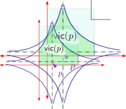
Figure 2.1: The green region is $[0,1]^{2}\cap\mathsf{vic}\left({p}\right)$. The light blue region is $[0,1]^{2}\setminus\mathsf{vic}\left({p}\right)$.

Lemma 2.9 ([CHR16]).

For any $p\in[0,1]^{d}$, we have $vol\left({\mathsf{vic}\left({p}\right)}\right)=O(\frac{\log^{d}n}{n})$.

Proof:

Let $\mathsf{o}$ denote the origin. The area of a single quadrant of the vicinity is maximized when $p=\mathsf{o}$. There are $2^{d}$ quadrants so we have that $vol\left({\mathsf{vic}\left({p}\right)}\right)\leq 2^{d}vol\left({\mathsf{vic}\left({\mathsf{o}}\right)}\right)$. To bound the later quantity, let $\tau>0$ be an integer such that $2^{d}\varphi\leq 2^{-\tau}\leq 2^{d+1}\varphi$. As such, we have $\tau\leq\lg(1/\varphi)-d=O(\log n).$

A canonical box, is a box of the form $B=\prod_{i=1}^{d}[0,\alpha_{i}]$ such that $vol\left({B}\right)=\prod_{i}\alpha_{i}=2^{-\tau}$, where $\alpha_{i}$ is a power of two, for all $i$. For any point $q=(q_{1},\ldots,q_{d})\in[0,1]^{d}$, let $\mathsf{p{}v}\left({q}\right)=\prod_{i=1}^{d}q_{i}$ be the point volume. Consider all the points of $q=(q_{1},\ldots,q_{d})\in\mathsf{vic}\left({\mathsf{o}}\right)$ (i.e., these are points with $\mathsf{p{}v}\left({q}\right)\leq\varphi$), and let $\left\lceil{q}\right\rceil_{2}=(\left\lceil{q_{1}}\right\rceil_{2},\ldots,\left\lceil{q_{d}}\right\rceil_{2})$. Observe that $\mathsf{p{}v}\left({\left\lceil{q}\right\rceil_{2}}\right)\leq 2^{d}\varphi$. In particular, there exists a canonical box that contains $q$.

Consider a side $[0,\alpha_{i}]$ of a canonical box. The number $\alpha_{i}$ is a power of $2$, and $1\geq\alpha_{i}\geq 2^{-\tau}$. That is, $\alpha_{i}\in\{1,1/2,1/4,\ldots,2^{-\tau}\}$. Namely, there are at most $1+\tau$ choices for the value of each coordinate of a canonical box. As such, the number of canonical boxes is $(1+\tau)^{d-1}$, as fixing $d-1$ coordinates forces the value of the last coordinate. The volume of a canonical box is $\leq 2^{d+1}\varphi$. We conclude $\mathsf{vic}\left({\mathsf{o}}\right)$ is covered by the union of these boxes, and as such, $vol\left({\mathsf{vic}\left({\mathsf{o}}\right)}\right)\leq\tau^{d-1}\varphi$, which implies the claim.  

The intuition for vicinities is that for a lot of the problems discussed in the introduction, any point $p\in P$ only needs to locally consider other points in its vicinity when making decisions of building the desired structures (i.e. points outside the vicinity of $p$ are not relevant for $p$)

3 Sharp concentration of the $k$th pairwise distance

Let $P=\left\{{p_{1},\ldots,p_{n}}\right\}$ be a random sequence of points, where $p_{i}$ is picked uniformly and independently from $[0,1]^{d}$. For two numbers $x,y\in[0,1]$ their toroidal distance is $\left|{x-y}\right|_{T}=\min\bigl{(}\left|{x-y}\right|,1-\left|{x-y}\right|\bigr{)}$. Let $r$ be a fixed value in $[0,1]$. Let $f_{r}(P)$ denote the number of pairs $p_{i}p_{j}$ in $P$ with $\left\|p_{i}p_{j}\right\|_{T}\leq r$. Formally, we have

$$\left\|p_{i}p_{j}\right\|_{T}=\sqrt{\sum\nolimits_{\ell=1}^{d}\left|{p_{i}[\ell]-p_{j}[\ell]\bigr{.}}\right|_{T}^{2}}\qquad\text{and}\qquad f_{r}(P)=\left|{\left\{p_{i}p_{j}\;\middle|\;i<j\text{ and }\left\|p_{i}p_{j}\right\|_{T}\leq r\right\}}\right|.$$ (3.1)

is the toroidal distance between $p_{i}$ and $p_{j}$, and $p[\ell]$ denotes the $\ell$th coordinate of a point $p\in\mathbb{R}^{d}$. We denote the space $[0,1]^{d}$ under this toroidal topology by $[0,1]^{d}_{T}$. Intuitively, this is the space where we allow “wrap-around” in $[0,1]^{d}$, and the shortest distance between two points can be the wrap-around distance. Using this distance allows us to ignore artifacts that are generated by the boundary of the hypercube $[0,1]^{d}$.

The claim is that the value of $f_{r}$, which is a number in $\{0,\ldots,\binom{n}{2}\}$, is strongly concentrated. Namely, the interval of integers containing $f_{r}$, with high probability, is “short”. Showing a bound of $\scalerel*{\widetilde{O}}{j^{2}}(n^{3/2})$ on the number of values in this interval is doable via Chernoff’s inequality and using the union bound. The resulting guarantee is of the form $\mathop{\mathbb{P}}\left[\left|{f_{r}-\mathop{\mathbb{E}}\!\left[{f_{r}}\right]}\right|>\scalerel*{\widetilde{\Omega}}{j^{2}}(n^{3/2})\right]\leq{1}/{n^{O(1)}}.$ Here, we show a significantly stronger concentration with the interval containing $\scalerel*{\widetilde{O}}{j^{2}}(n)$.

We conjecture this result is true for the Euclidean distance, but handling the boundary cases proved to be quite challenging. Hence the simplifying Toroidal topology assumption. We observed this strong concentration, for both the Toroidal and Euclidean case, in computer simulations.

Consider the closed ball $\mathcalb{b}_{T}\left({p,r}\right)=\left\{x\in[0,1]^{d}\;\middle|\;\left\|px\right\|_{T}\leq r\right\}$ in $[0,1]^{d}_{T}$. We next bound the VC dimension of such balls (as a side, Gillibert et al. [GLM22] bounded the VC-dimension of axis-parallel boxes in this space by $O(d\log d)$).

Lemma 3.1.

For $\mathcal{A}=\left\{\mathcalb{b}_{T}\left({p,r}\right)\;\middle|\;p\in\mathbb{R}^{d}\right\}$, the VC dimension of the range space $([0,1]^{d},\mathcal{A})$ is $O(1)$.

Proof:

A toroidal ball consists of at most $O(2^{2d})$ regions $R_{i}$, each region being the intersection of a ball and at most $2d$ half spaces (corresponding to the boundaries of $[0,1]^{d}$). The VC dimension of balls and halfspaces is $d+1$, so the VC dimension of their intersection (and hence each region) is $O(1)$. Taking the union of the at most $O(2^{2d})$ regions, implies the VC dimension is at most $O(1)$, via standard argumentation [Har11].  

Next, we would like to apply Chernoff-like style inequalities to bound the probability of deviation from the expectation. The most relevant inequality here is McDiarmid’s inequality for bounded differences of martingales. Unfortunately, one cannot use McDiarmid’s inequality directly because by “sliding” a ball $\mathcalb{b}$ in $[0,1]^{d}$, the number of points inside $\mathcalb{b}$ might change by $O(n)$. Of course for random point set $P$, this is highly unlikely (the change is more likely to be $O(\sqrt{n})$) and so we will have to use a variation of McDiarmid’s inequality that allows a “bad” event, where the difference might be large but happening with a small probability, and a “good” typical event where the difference is bounded.

Consider the following extension of McDiarmid’s inequality (for bounded differences of martingales) where the differences are only bounded with high probability [Kut02]. It will be useful to view $P$ from two different views, one as a set of individual points, and the second as a product $\Omega=\prod_{1\leq i\leq dn}\Omega_{i}$ of $dn$ probability spaces for each coordinate.

Definition 3.2 ([Kut02]).

Let $\Omega_{1},...,\Omega_{m}$ be probability spaces. Let $\Omega=\prod_{i}\Omega_{i}$, and let $X$ be a random variable on $\Omega$. The variable $X$ is strongly difference-bounded by $(b,c,\varsigma)$ if the following holds. There is a “bad” subset $B\subseteq\Omega$, where $\varsigma=\mathop{\mathbb{P}}\left[w\in B\right]$. In addition, we require that

1. If $\omega,\omega^{\prime}\in\Omega$ differ only in the $k$th coordinate, and $\omega\not\in B$ then $\left|{X(\omega)-X(\omega^{\prime})}\right|\leq c$.

2. Furthermore, for any $\omega,\omega^{\prime}\in\Omega$ differing only in the $k$th coordinate, $\left|{X(\omega)-X(\omega^{\prime})}\right|\leq b$.

To decipher this definition consider the case that $c<b$: the difference between “bad” pairs can be large, but the difference between “good” (or mixed) pairs is small. The quantity $b$ behaves like the “worst” case difference, $c$ is the “typical” difference, and $\varsigma$ is the probability of the bad event happening.

Lemma 3.3 ([Kut02], Corollary 3.4).

Let $\Omega_{1},...,\Omega_{m}$ be probability spaces. Let $\Omega=\prod_{1\leq i\leq m}\Omega_{i}$ and let $X$ be a random variable on $\Omega$ which is strongly difference-bounded by $(b,c,\varsigma)$. Let $\mu=\mathop{\mathbb{E}}\!\left[{X}\right]$. Then, for any $\tau>0$, and any $\alpha>0$, we have $\mathop{\mathbb{P}}\left[\bigl{.}\left|{X-\mu}\right|\geq\tau\right]\leq 2\Bigl{[}\exp{\bigl{(}-\frac{\tau^{2}}{2m(c+b\alpha)^{2}}\bigr{)}}+\frac{m}{\alpha}\varsigma\Bigr{]}.$

In the following, let $P+p=P\cup\{p\}$ and $P-p=P\setminus\{p\}$.

Lemma 3.4.

The random variable $f_{r}$ is strongly difference-bounded by

$$(b,c,\varsigma):=(n-1,O(\sqrt{n\log n}),{1}/{n^{O(1)}}).$$

Proof:

If one moves only one point of $P$, at most $n-1$ pairwise distances involved with this point can change, implying that $b\leq n-1$.

By the $\varepsilon$-sample theorem, and Lemma 3.1, a sample of size $O\bigl{(}\varepsilon^{-2}\log n\bigr{)}$ is an $\varepsilon$-sample for Toroidal balls, with high probability. Interpreting $P$ as an $\varepsilon$-sample for $[0,1]^{d}$, implies that this holds for $P$ with $\varepsilon=\sqrt{\varphi}=\sqrt{\frac{c_{d}\ln n}{n}}$ for sufficiently small constant $c_{d}>0$. Let $\mathcalb{v}_{d}=vol\left({\mathcalb{b}_{T}\left({q,r}\right)\bigr{.}}\right)$, for any point $q\in[0,1]^{d}$. The number of points in distance $\leq r$ from a point $p\in[0,1]^{d}$, is $X_{p}=\left|{P\cap\mathcalb{b}_{T}\left({p,r}\right)}\right|$. Hence, for any Toroidal ball we have

$$\left|{X_{p}-\mathop{\mathbb{E}}\!\left[{X_{p}}\right]}\right|=\left|{\bigl{.}\left|{P\cap\mathcalb{b}_{T}\left({p,r}\right)}\right|-\mathcalb{v}_{d}n}\right|\leq\varepsilon n=\sqrt{c_{d}n\log n}=\scalerel*{\widetilde{O}}{j^{2}}(\sqrt{n})$$ (3.2)

assuming $P$ is indeed an $\varepsilon$-sample. Note that the bound above crucially uses the Toroidal distance properties. Furthermore, the set $P-p$, formed by removing any point $p\in P$, is an $\varepsilon$-sample, and this holds with high probability for all such subsets.

This readily implies that for any two points $p,p^{\prime}\in[0,1]^{d}$, we have

$$\left|{X_{p}-X_{p^{\prime}}}\right|\leq\left|{X_{p}-\mathcalb{v}_{d}n}\right|+\left|{\mathcalb{v}_{d}n-X_{p^{\prime}}}\right|=O(\sqrt{n\log n}).$$

Picking a point $p\in P$, and a point $p^{\prime}\in[0,1]^{d}$, and setting $P^{\prime}=P-p+p^{\prime}$, we are interested in bounding the “typical” difference between $f_{r}(P)$ and $f_{r}(P^{\prime})$ (this would be the value of $c$). We have

$$\left|{f_{r}(P)-f_{r}(P^{\prime})}\right|\leq\left|{X_{p}-X_{p^{\prime}}}\right|+O(1)=O(\sqrt{n\log n}).$$

This implies that $c=O(\sqrt{n\log n})$. This calculation fails, only if $P$ fails to be an $\varepsilon$-sample, which happens with probability $\varsigma\leq 1/n^{O(1)}$.  

Theorem 3.5.

For constant $c^{\prime}$ sufficiently large, we have $\mathop{\mathbb{P}}\left[\left|{f_{r}-\mathop{\mathbb{E}}\!\left[{f_{r}}\right]}\right|>c^{\prime}n\log n\right]\leq{1}/{n^{O(1)}}.$

Proof:

This follows readily by plugging the parameters of Lemma 3.4 into Lemma 3.3. Note that in our case, $m=n,b=n-1$, and $c=\sqrt{c_{d}n\log n}$. Choosing $\alpha={1}/{n}$ and $\varsigma\leq{1}/{dn^{3}}$ (which can be ensured by making $c_{d}$ sufficiently large), and $\tau=\Omega(n\log n)$, the result follows by straightforward calculations from Lemma 3.3. For example, plugging $\tau=100\sqrt{c_{d}}n\log n$ into Lemma 3.3 yields (for sufficiently large $c_{d}$): $\displaystyle\mathop{\mathbb{P}}\left[\left|{f_{r}(P)-\mathop{\mathbb{E}}\!\left[{f_{r}(P)}\right]}\right|>100\sqrt{c_{d}d}n\log n\right]$ $\leq 2\bigl{[}\exp{\bigl{(}-\frac{10000c_{d}dn^{2}\log(n)^{2}}{2dn(2\sqrt{c_{d}n\log n}+1)^{2}}\bigr{)}}+\frac{dn^{2}}{dn^{3}}\bigr{]}\leq\frac{4}{n}.$  

4 Warm-up: Computing the convex hull in linear time

We present here an algorithm for computing the convex hull of $P$ in $O(n)$ time. This will serve as a warm-up as the tools here will be used later on.

Algorithm.

Given $P$, we build $T$, a quadtree of height $h=\lceil(\log_{2}n)/{d}\rceil$ and insert the points $P$ in $O(n)$ time to its leaves – this can readily be done by storing the points in the grid formed by the leafs using hashing (or just direct array indexing).

The algorithm computes the convex hull via a bottom-up traversal of the tree. It starts by computing the convex hull (potentially empty) for each leaf of the quadtree using any brute force algorithm. For a node $v$ at level $k$, the algorithm takes the computed convex-hulls of its children, extracts all their vertices and stores it in a set $S$, and computes the combined convex-hull of $S$, using off-the-shelf algorithm [Cha93] in $O(|S|\log|S|+|S|^{\left\lfloor{d/2}\right\rfloor})$ time.

Analysis.

The algorithm correctness is immediate. We next prove an inferior upper bound on the expected complexity of the random convex-hull that holds with higher moments.

Lemma 4.1.

Let $\left|{\mathcal{C}\left({P}\right)}\right|$ denote the number of vertices in the convex hull of $P$. For any integer $\kappa>0$, we have $\mathop{\mathbb{E}}\!\left[{\left|{\mathcal{C}\left({P}\right)}\right|^{\kappa}}\right]=O(\log^{O(\kappa d)}n)$ (the constant hidden by the $O$ depends on both $\kappa$ and $d$).

Proof:

Let $p$ be a vertex of the convex-hull $\mathcal{C}\left({P}\right)$, and consider a tangent (hyper)plane $h$ to $\mathcal{C}\left({P}\right)$ that passes through $p$. The plane $h$ separates $\mathcal{C}\left({P}\right)$ from one of the vertices of the $[0,1]^{d}$, say $q$. Let $R$ be the axis parallel box with $p$ and $q$ as antipodal vertices.

The VC dimension of axis aligned boxes is $2d$; see [Har11]. By the $\varepsilon$-net theorem, a sample of size $O(d\varepsilon^{-1}\log n)$ is an $\varepsilon$-net for axis aligned boxes, with probability $\geq 1-1/n^{O(d)}$. Setting $\varepsilon=\varphi=c_{d}(\log n)/n$, it follows that $R$ contains a point of $P$ with high probability. It follows that all the vertices of $\mathcal{C}\left({P}\right)$ are in the vicinity of some vertex of $[0,1]^{d}$. Let $\Xi$ be the union of the vicinities of the vertices of $[0,1]^{d}$. By Lemma 2.9, we have that $\alpha=vol\left({\Xi}\right)=O((\log n)^{d}/n)$. Applying Lemma 2.8 to $|\Xi\cap P|^{\kappa}$ now implies the claim.  

Lemma 4.2.

The above algorithm computes $\mathcal{C}\left({P}\right)$ is $O(n)$ expected time.

Proof:

Consider the root of the quadtree – it has $2^{d}$ children, and let $P_{i}$ be the set of points of $P$ stored in the $i$th child. Let $n_{i}=|P_{i}|$ and $m_{i}=|V\left({\mathcal{C}\left({P_{i}}\right)}\right)|$. We have that $\sum_{i}n_{i}=n$, and $\mathop{\mathbb{E}}\!\left[{n_{i}}\right]=n/2^{d}$. In particular, using Chernoff’s inequality we have that $n_{i}\leq(7/8)n$ with high probability. Similarly, we have that $\mathop{\mathbb{E}}\!\left[{m_{i}^{\kappa}}\right]=O(\log^{O(\kappa d)}n)$ by Lemma 4.1. Let $m=\sum_{i}m_{i}$, and observe that computing the convex-hull at the top most level takes $O(m\log m+m^{\left\lfloor{d/2}\right\rfloor})=O(m^{d})=O(2^{d}\sum_{i}m_{i}^{d})$. Thus, ignoring the construction time of the quadtree itself, we have the recurrence

$$T(n)=O\left({\mathop{\mathbb{E}}\!\left[{\smash{\textstyle\sum\nolimits_{i}m_{i}^{d}}\bigr{.}}\right]}\right)+\sum_{i}T(n_{i})=\log^{O(d^{2})}n+\sum_{i}T(n_{i}),$$

and the solution to this recurrence is $O(n)$.  

5 Complexity of the Delaunay triangulation of random points

Here we show that the Delaunay triangulation of $P$ has linear complexity in expectation.

Background on Delaunay triangulations.

A simplicial complex $\mathcal{D}$ over a set $P$ is a set system with the (hyper) edges being subsets of $P$, such that for any $\sigma,\sigma^{\prime}\in\mathcal{D}$, we have that $\sigma\cap\sigma^{\prime}\in\mathcal{D}$. An edge of $\mathcal{D}$ is a simplex. A simplex is $k$ dimensional if the affine space its points span is $k$ dimensional. Simplices of dimension $0,1$ and $2$ are vertices, edges and (two dimensional) faces, respectively.

For a point $p\in\mathbb{R}^{d}$, and a radius $r>0$, let $\mathcalb{b}\left({p,r}\right)$ denote the open ball of radius $r$ centered at $p$. For any points $p_{1},\ldots,p_{k}\in\mathbb{R}^{d}$, let $\mathsf{pen}\left({p_{1},\ldots,p_{k}}\right)$ denote the pencil of $p_{1},\ldots,p_{k}$: the set of all open balls $\mathcalb{b}$ in $\mathbb{R}^{d}$, such that their boundary sphere passes through $p_{1},\ldots,p_{k}$. If $k=d+1$, and the points are in general position, the pencil is a single ball $\mathsf{circum}\left({p_{1},\ldots,p_{k}}\right)$ bounded by the circumscribed sphere of these points.

The Delaunay triangulation $\mathcal{D}=\mathcal{D}(P)$ of $P$ is a simplicial complex, where $\nabla\in\mathcal{D}$ $\iff$ there is a ball $\mathcalb{b}\in\mathsf{pen}\left({\nabla}\right)$ such that $\mathcalb{b}\cap P=\emptyset$. The Delaunay triangulation has the property that if the set of points $P$ is a random set then the points are in general position with probability $1$ (i.e., almost surely), and it is then uniquely defined.

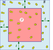
Figure 5.1: The inner fortress $\mathcal{F}$ in red. The moat $\mathcal{M}$ in light blue. Here $\delta=\sqrt[d]{\frac{c_{d}\ln n}{n}}$.

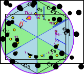
Figure 5.2: Definitions of $\mathcalb{n}_{i}=\mathcalb{n}_{\mathcalb{c}_{i}}\left({p}\right)$ and $\ell\left({p}\right)$.

5.1 A linear bound in the interior of the hypercube

Let $\mathcal{F}=[\delta,1-\delta]^{d}$ be the fortress of $[0,1]^{d}$, and $\mathcal{M}=[0,1]^{d}\setminus\mathcal{F}$ be its moat, where $\delta=\sqrt[d]{\frac{c_{d}\ln n}{n}}$. See Eq. (2.1) and Figure 5.1.

Definition 5.1.

Consider a ray emanating from a point $q$ in a direction $v$ in $\mathbb{R}^{d}$. A cone of angle $\alpha$ is the set of all points $p\in\mathbb{R}^{d}$, such that the angle between $p-q$ and $v$ is at most $\alpha$. The point $q$ is the apex of the cone.

One can cover space around a point with $O_{d}(1)$ cones, with angle $\pi/12$, to cover all of $\mathbb{R}^{d}$

Lemma 5.2 ([DGL96]).

For any point $p\in\mathbb{R}^{d}$, one can construct a set $\mathcalb{C}_{p}$ of $2^{O(d)}$ cones with apex $p$ and angle $\pi/12$, such that $\cup\mathcalb{C}_{p}=\mathbb{R}^{d}$.

The following shows that all these cones are not empty, if the apex $p$ is in the fortress.

Lemma 5.3.

For any $p\in\mathcal{F}$, and any cone $\mathcalb{c}\in\mathcalb{C}_{p}$, we have $\mathop{\mathbb{P}}\left[\mathcalb{c}\cap(P-p)=\emptyset\right]<1/n^{O(1)}$.

Proof:

Since $p\in\mathcal{F}$, it is at a distance of at least $\delta$ from the boundary of $[0,1]^{d}$. Thus, $\alpha=vol\left({\mathcalb{c}\cap[0,1]^{d}}\right)$ $=\Omega(\delta^{d})=\Omega(\varphi)=\Omega\bigl{(}(\log n)/n\bigr{)}$, by Eq. (2.1). This implies that the probability that $\mathcalb{c}$ does not contain any of the points of $P-p$ is at most

$$(1-\alpha)^{n-1}\leq\exp\left({\bigl{.}-\alpha(n-1)}\right)\leq\exp\left({-c\ln n}\right)=\frac{1}{n^{O(1)}},$$

where $c$ is a constant that can be made to be arbitrarily large by increasing the value of $c_{d}$. The result now follows by applying the union bound to all the cones in $\mathcalb{C}_{p}$.  

Definition 5.4.

For a point $p\in P\cap\mathcal{F}$ and a cone $\mathcalb{c}\in\mathcalb{C}_{p}$, let $\mathcalb{n}_{\mathcalb{c}}\left({p}\right)$ denote the nearest neighbor to $p$ in $\mathcalb{c}\cap(P-p)$. The reach of $p$ is $\ell\left({p}\right)=\max_{\mathcalb{c}\in\mathcalb{C}_{p}}\left\|p\mathcalb{n}_{\mathcalb{c}}\left({p}\right)\right\|,$ see Figure 5.

The following bounds (in expectation) $\ell(p)$ and the distance between $p$ and $\mathcalb{n}_{\mathcalb{c}}\left({p}\right)$ for $\mathcalb{c}\in\mathcalb{C}_{p}$.

Lemma 5.5.

For any point $p\in P\cap\mathcal{F}$, a cone $\mathcalb{c}\in\mathcalb{C}(p)$ and $t\leq\delta$, we have:

1. $\mathop{\mathbb{P}}\left[\left\|p\mathcalb{n}_{\mathcalb{c}}\left({p}\right)\right\|>t\right]\leq\exp(-c\,t^{d}n)$, where $c$ is constant that depends only on the dimension.

2. $\mathop{\mathbb{P}}\left[\ell\left({p}\right)>t\right]\leq f(t,n)=\exp\bigl{(}O(d)-c\,t^{d}n\bigr{)}$,

3. $\mathop{\mathbb{E}}\!\left[{\ell\left({p}\right)}\right]=\Theta(1/\sqrt[d]{n})$, and

4. the reach of all the points of $P\cap\mathcal{F}$ is bounded by $\delta$, with probability $1/n^{O(d)}$.

Proof:

(I) If $\left\|p\mathcalb{n}_{\mathcalb{c}}\left({p}\right)\right\|>t$ then the set $R=\mathcalb{c}\cap\mathcalb{b}\left({p,t}\right)$ contains no points of $P$. The volume of $\mathcalb{c}\cap\mathcalb{b}\left({p,t}\right)$, for $t\leq\delta$, is $\alpha=\Omega(t^{d})$. In this case, all the points of $P-p$ must avoid $R$. This happens with probability at most $(1-\alpha)^{n-1}\leq\exp\bigl{(}-\alpha(n-1)\bigr{)}\leq\exp\bigl{(}-ct^{d}n\bigr{)}$.

(II) By the union bound, and Lemma 5.2, we have $\Bigl{.}\mathop{\mathbb{P}}\left[\ell\left({p}\right)>t\right]\leq\sum_{\mathcalb{c}\in\mathcalb{C}(p)}\mathop{\mathbb{P}}\left[\mathcalb{n}_{\mathcalb{c}}\left({p}\right)>t\right]\leq f(t,n).$

(III) Observe that $\mathcalb{b}\left({p,1/2\sqrt[d]{n}}\right)$ contains no other points of $P-p$ with constant probability. This implies that $\mathop{\mathbb{E}}\!\left[{\ell\left({p}\right)}\right]=\Omega(1/\sqrt[d]{n})$. The upper bound $\mathop{\mathbb{E}}\!\left[{\ell\left({p}\right)}\right]=O(1/\sqrt[d]{n})$ follows by the above exponential decay, as a straightforward calculation shows.

(IV) Setting $t=\delta$, and using the union bound implies this part.  

Definition 5.6.

For $p\in P\cap\mathcal{F}$, the influence of $p$ is $\varocircle_{p}=\left\{q\in P\;\middle|\;\left\|pq\right\|\leq 2\ell\left({p}\right)\right\}$

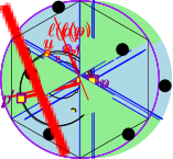
Figure 5.3: Sketch of proof of Lemma 5.7

Importantly, all the Delaunay edges adjacent to a point $p\in\mathcal{F}$ are contained in $p$’s region of influence. Hence, locally, it is sufficient to only consider points in the influence when computing the Delaunay triangulation.

Lemma 5.7.

For any point $p\in P\cap\mathcal{F}$, If $pq\in\mathcal{D}$, then $q\in\varocircle_{p}$.

Proof:

Consider the largest (open) ball $\mathcalb{b}$ with $p$ on its boundary, that does not contain any point of $P$ in its interior, and let $r$ be its radius and $z$ be its center, see Figure 5.3. We claim that $r\leq\ell\left({p}\right)$, which would imply that $\left\|pq\right\|\leq 2r\leq 2\ell\left({p}\right)$. Assume that $r>\ell\left({P}\right)$, and consider any cone $\mathcalb{c}\in\mathcalb{C}_{p}$, such that $z\in\mathcalb{c}$. Let $p^{\prime}$ be the diametrical point on $\partial\mathcalb{b}$ to $p$. Consider any point $u\in\mathcalb{c}\setminus\mathcalb{b}$. The distance $pu$ is minimized if $u\in\partial\mathcalb{b}$, but then $\angle pup^{\prime}$ forms the right angle of a right triangle. Observe that $\angle upp^{\prime}<30^{\circ}$ since the cone angle is at most $30^{\circ}$. But then

$$\left\|pu\right\|=\left\|pp^{\prime}\right\|\cos\angle p^{\prime}pu=2r\cos\angle p^{\prime}pu>2\ell\left({p}\right)\cos 30^{\circ}=(2\sqrt{3}/2)\ell\left({p}\right)>\ell\left({p}\right).$$

However, $\mathcalb{b}\cap(P-p)=\emptyset$ implies that the closest point in $(P-p)\cap\mathcalb{c}$ to $p$ has distance larger than $\ell\left({p}\right)$, which contradicts the definition of $\ell\left({p}\right)$.  

We next bound the moments of the size of the set of points inside the influence of a point.

Lemma 5.8.

For $p\in P\cap\mathcal{F}$, and any constant $\kappa\geq 1$, we have $\mathop{\mathbb{E}}\!\left[{|\varocircle_{p}|^{\kappa}\bigr{.}}\right]=O_{\kappa}(1)$, see Definition 5.6.

Proof:

Let $L=\left|{\varocircle_{p}}\right|$. We break $P$ into two roughly equal sets $P_{1}$ and $P_{2}$ (this is done before sampling the locations of the points). Let $\ell_{i}=\ell\left({p,P_{i}}\right)$ be the reach of $p$ in $P_{i}$ for $i\in\{1,2\}$. Arguing as above, as $p\in\mathcal{F}$, this quantity is well defined. Let $U_{i}$ be the number of points of $P_{3-i}$ in the ball $\mathcalb{b}_{i}=\mathcalb{b}\left({p,\ell_{i}}\right)$. Clearly, $\mathop{\mathbb{E}}\!\left[{L}\right]\leq\mathop{\mathbb{E}}\!\left[{U_{1}}\right]+\mathop{\mathbb{E}}\!\left[{U_{2}}\right]$, as $\mathcalb{b}_{i}$ contains more points of $P_{3-i}$ than the ball defined by the reach of the whole set.

So, let $\psi$ be the minimum value such that $f(\psi,n/2)\leq 1/2$, where $f$ is the function defined in Lemma 5.5. It is easy to verify that $\psi=O(1/n^{1/d})$. Let $\mathcalb{b}_{0}=\mathcalb{b}\left({p,\psi}\right)$, and, for $i>0$, let $\mathcalb{r}_{i}=\mathcalb{b}\left({p,i\psi}\right)\setminus\mathcalb{b}\left({p,(i-1)\psi}\right)$. Observe that $vol\left({\mathcalb{b}_{0}}\right)=O(1/n)$, and $vol\left({\mathcalb{r}_{i}}\right)=O(i^{d}/n)$. By Lemma 2.8, we have that $N_{0}=\mathop{\mathbb{E}}\!\left[{\bigl{.}|P_{2}\cap\mathcalb{b}_{0}|^{\kappa}}\right]=O(1)$, and $N_{i}=\mathop{\mathbb{E}}\!\left[{|P_{2}\cap\mathcalb{r}_{i}|^{\kappa}}\right]=O(i^{d\kappa})$. We have that $\mathop{\mathbb{E}}\!\left[{L^{\kappa}\bigr{.}}\right]=O(T)$, where

$$T=\sum_{i=0}^{\infty}N_{i}\mathop{\mathbb{P}}\left[\ell>i\psi\right]\leq\sum_{i=0}O_{\kappa}(i^{\kappa d}f(i\psi,n/2))=\sum_{i=0}O_{\kappa}(i^{\kappa d}/2^{i})=O_{\kappa}(1),$$

since $f(i\psi,n/2)=\exp\bigl{(}O(d)-c\,i^{d}\psi^{d}n\bigr{)}\leq\left({\exp\bigl{[}O(d)-c\,\psi^{d}n\bigr{]}}\right)^{i^{d}}\leq 1/2^{i^{d}}.$  

Combining everything, we get the main result for points in the fortress.

Lemma 5.9.

Let $\mathcal{D}$ be the Delaunay triangulation of $P$. The expected number of simplices that include any point of $P\cap\mathcal{F}$ is $O(n)$.

Proof:

Let $\tau=|\varocircle_{p}|$. All the vertices of a simplex of the Delaunay triangulation containing $p$ must have all its vertices in $\varocircle_{p}$ by Lemma 5.7. Thus, the number of such simplices, of all dimensions, is bounded by $\sum_{i=0}^{d+1}\binom{\tau}{i}=O(\tau^{d})$. By Lemma 5.8, we have $\mathop{\mathbb{E}}\!\left[{O(\tau^{d})}\right]=O(1)$.  

5.2 The complexity of the Delaunay triangulation near the boundary

We are now left with the tedious technicality of handling points that are too “close” to the boundary. The idea is to use a similar argumentation to the above, but to replace the influence ball induced by the reach by a different region. This inflated region contains significantly more points, but since the number of points in the moat is small, this would still be linear overall. We remind the reader that the moat is the area $\mathcal{M}=[0,1]^{d}\setminus[\delta,1-\delta]^{d}$, see Figure 5.1 and Eq. (2.1).

The following is an immediate consequence of Lemma 2.8 and Lemma 2.9.

Lemma 5.10.

For any point $p\in P$, we have $X=\left|{\mathsf{vic}\left({p}\right)\cap P}\right|=O(\log^{d}n)$ with probability $\geq 1-1/n^{O(1)}$.

Lemma 5.11.

Consider an axis parallel box $B=\prod_{i=1}^{d}[p_{i},q_{i}]$, and assume that there is a ball $\mathcalb{b}$ that contains the points $p=(p_{1},\ldots,p_{d})$ and $q=(q_{1},\ldots,q_{d})$. Then $\mathcalb{b}$ contains a $d$-dimensional simplex $\nabla$ defined by $d+1$ vertices of $B$, such that the volume of this simplex is $\geq vol\left({B}\right)/d!$. More generally, this holds for any ball that contains two diametrical vertices of $B$.

Proof:

The proof is by induction on $d$. The claim is immediate if $d=1$.

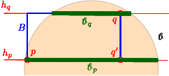
Figure 5.4:

For $d>1$, the idea it to provide a path along the edges of the box $B$ between the two vertices that is contained in $\mathcalb{b}$ – the convex-hull of this path would provide the desired simplex. So, consider the two hyperplanes $h_{p}\equiv x_{d}=p_{d}$ and $h_{q}\equiv x_{d}=q_{d}$, see Figure 5.4. Consider the two balls $\mathcalb{b}_{p}=\mathcalb{b}\cap h_{p}$ and $\mathcalb{b}_{q}=\mathcalb{b}\cap h_{q}$. Both balls have the same center if we ignore the $d$th coordinate, and one of them must have a bigger (or equal) radius to the other. Assume that $\mathcalb{b}_{p}$ has the bigger radius, and observe that it as such must contain the point $q^{\prime}=(q_{1},\ldots,q_{d-1},p_{d})$. This implies that the segment $qq^{\prime}\subseteq\mathcalb{b}$. By induction there is a path on the edges of $B\cap h_{p}$ between $p$ and $q^{\prime}$, which implies that there is a path on the edges of $B$ between $p$ and $q$ that lies inside $\mathcalb{b}$.  

For points $p\in\mathcal{M}$, as the following testifies, one needs to consider only simplices and points that are in $\mathsf{vic}\left({p}\right)$. This is indeed a larger region than the influence region used before, but is small enough for our purposes.

Lemma 5.12.

Let $p$ be any point in $P$. With high probability, there are at most $O(\log^{d^{2}}n)$ simplices in $\mathcal{D}=\mathcal{DT}\left({P}\right)$ that contains $p$ as a vertex. Furthermore, all the points neighboring $p$ in $\mathcal{D}$ must be in $\mathsf{vic}\left({p}\right)$, with probability $\geq 1-1/n^{O(d)}$.

Proof:

The VC dimension of simplices in $\mathbb{R}^{d}$ is $O(d^{2}\log d)$ as it is the intersection of $d+1$ halfspaces, each of VC dimension $d+1$, see [Har11]. By the $\varepsilon$-net theorem, a sample of size $O\bigl{(}(d^{2}\log d)\varepsilon^{-1}\log n\bigr{)}$ is an $\varepsilon$-net for simplices, with high probability. Interpreting $P$ as an $\varepsilon$-sample for $[0,1]^{d}$, implies that this holds for $P$ with $\varepsilon=\varphi/d!$, where $\varphi=(c_{d}\ln n)/n$, see Eq. (2.1) (by making $c_{d}$ sufficiently large).

Consider a point $q\in P$, such that $q\notin\mathsf{vic}\left({p}\right)$, and assume that $pq\in\mathcal{DT}\left({P}\right)$. This implies that there is a close ball $\mathcalb{b}$ that has $p$ and $q$ on its boundary, and no other points of $P$ in its interior. By Lemma 5.11, there is an (open) simplex $\nabla$ of volume $\geq vol\left({\mathsf{R}\left({p,q}\right)}\right)/d!\geq\varepsilon$ that contains $p$ and $q$ on its boundary, and it is contained inside $[0,1]^{d}\cap\mathcalb{b}$. But since $P$ is an $\varepsilon$-net for simplices, it follows that there is a point of $P$ in $\nabla$, which is a contradiction.

We conclude that all the edges adjacent to $p$ in $\mathcal{D}$ must be to points in $\mathsf{vic}\left({p}\right)$. But there are at most $t=O(\log^{d}n)$ such points, by Lemma 5.10. Since any simplex involving $p$ in $\mathcal{D}$ must use only points that are in the vicinity, it follows that the number of simplices (of all dimensions) adjacent to $p$ in $\mathcal{D}$ is bounded by $\sum_{i=0}^{d}\binom{t}{i}=O(t^{d})$.  

Finally, we show that the complexity of the Delaunay triangulation in the moat is sublinear.

Lemma 5.13.

Let $\mathcal{D}$ be the Delaunay triangulation of $P$. The expected number of simplices in $\mathcal{D}$ that include any point of $P\cap\mathcal{M}$ is $o(n)$.

Proof:

We have $\alpha=vol\left({\mathcal{M}}\right)\leq 2d\delta=O(\sqrt[d]{(\log n)/n})$, see Eq. (2.1). Thus, the expected number of points of $P$ in $\mathcal{M}$ is $\alpha n=O(n^{1-1/d}\log n)$. (As usual, this bound holds with high probability.) By Lemma 5.12, the total number of simplices in the Delaunay triangulation of $P$ involving points in the moat is bounded by $O(\alpha n\log^{O(d^{2})}n)=o(n)$, with high probability.  

The result.

Combining Lemma 5.9 and Lemma 5.13 implies the following.

Theorem 5.14.

For fixed $d$, the complexity of the Delaunay triangulation of a set of $n$ random points picked uniformly and independently in $[0,1]^{d}$ is $O(n)$ in expectation.

6 Constructing the Delaunay triangulation in linear time

6.1 Algorithm

We established above that the (expected) complexity of the Delaunay triangulation is linear by giving a (linear sized) superset of vertices/simplices that are a superset of the features of $\mathcal{D}$. We are now left with the task of extracting the features that do appear in $\mathcal{D}$. Recall, that the input is a set $P$ of $n$ random points from $[0,1]^{d}$.

I: Computing the Delaunay simplices attached to points in $P\cap\mathcal{F}$.

Let $N=\left\lceil{n^{1/d}}\right\rceil$. The algorithm throws the points of $P$ into a $N\times\cdots\times N$ uniform grid covering $[0,1]^{d}$. This can be done in linear time using hashing, where one can retrieve a list of all the points stored in a grid cell in constant time. Here a grid cell is uniquely represented by an integer tuple from $\{0,1\ldots,N-1\}^{d}$. Formally, we map a point $p=(p_{1},\ldots,p_{d})\in[0,1)^{d}$, to the grid cell with id $\mathsf{id}\left({p}\right)=(\left\lfloor{p_{1}N}\right\rfloor,\ldots,\left\lfloor{p_{d}N}\right\rfloor)$; see [Har11].

For a point $p\in P\cap\mathcal{F}$, the algorithm computes the reach $\ell\left({p}\right)$ by performing a marching cubes algorithm computing the intersection of the grid with the ball $\mathcalb{b}\left({p,r_{i}}\right)$, where initially $r_{i}=2^{i}/N$, for $i=0,1,\ldots$. The algorithm uses scanning to compute the point set $Q_{i}=\mathcalb{b}\left({p,r_{i}}\right)\cap P$ by extracting all the points stored in the intersecting grid cells. The algorithm stops in the $i$th iteration, if all cones in $\mathcalb{C}_{p}$ contains at least one point of $P$. At this point one can compute the reach of $p$ by computing for each cone $\mathcalb{c}\in\mathcalb{C}_{p}$ the closest point in $\mathcalb{c}\cap P_{i}$ to $p$. The algorithm then computes the point set $P_{p}=P\cap\mathcalb{b}\left({p,2r_{i}}\right)$, and computes the Delaunay triangulation of $P_{p}$ using any standard algorithm for computing Delaunay triangulation. Finally, the algorithm extract the star of $p$ from the computed triangulation, and store it. As a reminder, the star of $p$, denoted by $\hexstar_{p}$, is the set of all the simplices in the triangulation that contains $p$. The algorithm repeats this process for all the points of $P\cap\mathcal{F}$, and returns the union of all the stars computed.

II: Computing the Delaunay simplices attached to points in $P\cap\mathcal{M}$.

The algorithm builds an orthogonal range searching data structure on the points $P\cap\mathcal{M}$ (and not on all the whole point set $P$). Next, for each $p\in P\cap\mathcal{M}$, the algorithm constructs the set of $O(\log^{d-1}n)$ canonical boxes $\mathcal{B}_{p}$ (as defined in the proof of Lemma 2.9) that their union covers $\mathsf{vic}\left({p}\right)$. Then for each $\mathsf{r}\in\mathcal{B}_{p}$, it queries the data structure for points set $P_{\mathsf{r}}=\mathsf{r}\cap\mathcal{M}\cap P$. Next, it loops over $q\in P_{\mathsf{r}}$ and adds points in $P_{\mathsf{r}}\cap\mathsf{vic}\left({p}\right)$ to the computed set $N_{\mathcal{M}}(p)=P\cap\mathcal{M}\cap\mathsf{vic}\left({p}\right)$. Next, using the above grid, it computes the set $N_{\mathcal{F}}(p)=P\cap\mathcalb{b}\left({p,2\delta}\right)$. Finally, the algorithm computes the Delaunay triangulation of $P_{p}=N_{\mathcal{M}}(p)\cup N_{\mathcal{F}}(p)$ using a standard algorithm and extracts the star $\hexstar_{p}$ of $p$, from the computed triangulation, and stores it. The algorithm repeats this for each $p\in P\cap\mathcal{M}$ and returns the union of all stars computed for all $p$.

6.2 Analysis

In the following, we prove that the output of the algorithm is correct with probability $\geq 1-1/n^{O(d)}$ and the expected running time is $O(n)$.

Part I: The fortress.

The correctness of the algorithm is implied by the following claim.

Lemma 6.1.

For $p\in P\cap\mathcal{F}$, we have that $\nabla\in\hexstar_{p}$ if and only if $\nabla\in\mathcal{DT}\left({P}\right)$.

Proof:

If $\nabla\in\mathcal{DT}\left({P}\right)$, then by Lemma 5.7, $\nabla\subseteq\varocircle_{p}$. This implies that $\nabla\in\mathcal{DT}\left({\varocircle_{p}}\right)$, which implies that $\nabla$ is in the computed set $\hexstar_{p}$.

If $\nabla\in\hexstar_{p}$, then the circumball of $\nabla$ does not contain any point of $\varocircle_{p}$ in its interior. If this ball contained any point of $P$ in its interior, then it must be further than $2\ell\left({p}\right)$, but this is not possible by the argument used in the proof of Lemma 5.7.  

Lemma 6.2.

The above algorithm runs in expected $O(n)$ time.

Proof:

The Delaunay triangulation of $n$ points in $\mathbb{R}^{d}$, can be computed in $O(n^{\left\lceil{d/2}\right\rceil}+n\log n)=O(n^{d})$ [Mul94]. As such, we have that the expected running time is $\mathop{\mathbb{E}}\!\left[{\sum_{p\in P\cap\mathcal{F}}O(|\varocircle_{p}|^{d})}\right]=O(n),$ by Lemma 5.8.  

II: The moat.

Let $\mathcal{DT}\left({P}\right)_{\mathcal{M}}$ denote the set of simplices in $\mathcal{DT}\left({P}\right)$ with some vertices in $\mathcal{M}$. The correctness of the algorithm is implied by the following.

Lemma 6.3.

For all $p\in P\cap\mathcal{M}$, we have $\nabla\in\hexstar_{p}$ if and only if $\nabla\in\mathcal{DT}\left({P}\right)_{\mathcal{M}}$ with probability $\geq 1-1/n^{O(d)}$.

Proof:

Consider a simple $\nabla\in\mathcal{DT}\left({P}\right)_{\mathcal{M}}$ with $p\in V\left({\nabla}\right)$. If $\nabla$ contains a point $q\in V\left({\nabla}\right)$ that is in the fortress $\mathcal{F}$, and is outside $\mathcalb{b}\left({p,2\delta}\right)$, then $\ell\left({q}\right)>\delta$, and Lemma 5.5 implies that this happens with probability $<1/n^{O(d)}$. Thus, we have that $V(\nabla)\subseteq P\cap\bigl{(}(\mathcal{M}\cap\mathsf{vic}\left({p}\right))\cup\mathcalb{b}\left({p,2\delta}\right)\bigr{)}\subseteq P_{p}$. Thus, the empty ball $\mathcalb{b}$ in $\mathcal{DT}\left({P}\right)_{\mathcal{M}}$ that circumscribes $\nabla$ is still empty in $P_{p}$, $V\left({\nabla}\right)\subseteq P_{p}$, and thus $\nabla\in\hexstar_{p}$.

If $\nabla\in\hexstar_{p}$, then there is an empty ball $\mathcalb{b}$ that circumscribes $\nabla$ and is a witness to this. Assume for the sake of contradiction that $\mathcalb{b}$ is not empty, and let $q$ be the closest point to $p$ in $\mathcalb{b}\cap(P\setminus P_{p})$. If $q\in\mathcal{M}$, then $q\notin\mathsf{vic}\left({p}\right)$ (as $P\cap\mathcal{M}\cap\mathsf{vic}\left({p}\right)\subseteq P_{p}$). The probability for that this happens is $<1/n^{O(d)}$ by Lemma 5.12. If $q\in\mathcal{F}$, then the cone $\mathcalb{c}\in\mathcalb{C}_{q}$ that contains $p$, can not contain any closer point to $q$ (than $p$) from $P$. Namely, the reach of $q$ is bigger than $2\delta$, and probability for that is $\leq 1/n^{O(d)}$, by Lemma 5.5.  

Lemma 6.4.

The above algorithm runs in expected $O(n)$ time.

Proof:

We have $n_{\mathcal{M}}=\mathop{\mathbb{E}}\!\left[{|P\cap\mathcal{M}|}\right]\leq n\cdot d\cdot\delta=O(n^{1-1/d}\log n)$. Building the orthogonal range searching data-structure of $P\cap\mathcal{M}$ takes $O(n+n_{\mathcal{M}}\log^{d}n)=O(n)$.

For any $p\in P\cap\mathcal{M}$, computing $\mathcalb{b}\left({p,2\delta}\right)\cap P$ (using the grid) takes $O(\log n)$ time (and this bound holds with high probability). Computing the points in the vicinity of $p$ in the moat takes $O(\log^{O(d)}n)$ time – indeed each orthogonal range query takes $O(\log^{d}n)$ time, and there are $O(\log^{d}n)$ such queries. Finally, the time to compute the Delaunay triangulations $P_{p}$, is $O(\log^{O(d^{2})}n)$.

Putting everything together, we have that the expected running time of the second part of the algorithm is $O(n+n_{\mathcal{M}}\log^{O(d^{2})}n)=O(n)$.  

Theorem 6.5.

For fixed $d$, and a uniformly and independently sampled point set $P\subseteq[0,1]^{d}$ of size $n$, the above algorithm computes the Delaunay triangulation $\mathcal{DT}\left({P}\right)$ of $P$ in expected $O(n)$ time. The algorithm succeeds with high probability.

7 Constructing the MST in linear time

7.1 Preliminaries

Lemma 7.1.

Let $\mathcal{T}$ be the MST of $P$. The longest edge in $\mathcal{T}$ has length $\leq\delta=\sqrt[d]{c_{d}(\log n)/n}$ (see Eq. (2.1)), with probability $\geq 1-1/n^{O(d)}$, where $c_{d}$ is a sufficiently large constant.

Proof:

Let $pq$ be the longest edge in $\mathcal{T}$. Observe that diametrical ball $\mathcalb{b}$ defined by $p$ and $q$ can not contain any points of $P$ in its interior, as such a point $z$, would induce a cycle $pzq$ with $pq$ being the longest edge, which implies that it is not the MST. The volume of $\mathcalb{b}$ is minimized if its center lies in one the corners of $[0,1]^{d}$. We conclude that the region $R=\mathcalb{b}\cap[0,1]^{d}$ has $vol\left({R}\right)=\Omega_{d}(\left\|pq\right\|^{d}/2^{d})=\Omega_{d}(\left\|pq\right\|^{d}).$ Furthermore, $R$ is formed by the intersection of a hyperbox with ball, and the VC dimension of such ranges is $O(d)$ [Har11]. The point set $P$ can be interpreted as an $\varepsilon$-net for such ranges, with $\varepsilon=\delta^{d}/2^{d}=\Omega_{d}\bigl{(}(\log n)/n)$, with high probability. We conclude that if $\left\|pq\right\|\geq\delta$, then $P$ fails as an $\varepsilon$-net, which implies the claim.  

Definition 7.2.

The Yao graph $G_{\angle}=G_{\angle}\left({P}\right)$ [Yao82] of $P$ formed by connecting two points $p,q\in P$ by an edge if $q$ is the nearest point to $p$ in one of the cones of $\mathcalb{C}(p)$ (see Lemma 5.2). Let $G_{\angle,\delta}\left({P}\right)$ be the graph $G_{\angle}$ after removing from it all the edges with length $\geq\delta$.

It is well known that this graph contains the MST of $P$ [Yao82].

Lemma 7.3.

Let $P$ be a set of $n$ points picked uniformly at random from $[0,1]^{d}$. One can compute the graph $G_{\angle,\delta}\left({P}\right)$ in $O(n)$ expected time.

Proof:

We store the points of $P$ in a uniform grid with roughly $\Theta(n)$ cells in $[0,1]^{d}$. For every point $p\in P$, and every cone $\mathcalb{c}\in\mathcalb{C}_{p}$, we perform a marching cube algorithm to compute the closest point to $p$ in $\mathcalb{c}\cap P$. If the search distance exceeds $\delta$, we abort the search.

For a point $p$ in the fortress $\mathcal{F}$, computing the edges around $p$ takes $O(1)$ time in expectation, by Lemma 5.8. For points in the moat, their number is $O(n^{1-1/d}\log n)$, with high probability, and the search for each point is truncated after the distance exceeds $\delta$. Per point, such a search takes $O(\log n)$ time. It follows that the overall expected running time is $O(n+n^{1-1/d}\log^{2}n)=O(n)$.  

A refresher on Borůvka’s algorithm.

Let $G=(V,E)$ be an undirected graph with $n$ vertices and $m\geq n$ edges, and weights on the edges. Borůvka’s algorithm creates an empty forest $F_{0}$ over the vertices. Let $\mathsf{C}_{i-1}$ be the set of connected components of $F_{i-1}$. For $p\in P$, let $\sigma_{i-1}(v)\in\mathsf{C}_{i-1}$ denote the connected component of $v$ in $F_{i-1}$. While $|\mathsf{C}_{i-1}|\geq 2$, for each connected component $C\in\mathsf{C}_{i-1}$, the algorithm adds the cheapest edge leaving $V\left({C}\right)$ to some other connected component of $F_{i-1}$. Let $F_{i}$ be the resulting forest from $F_{i}$ after adding these edges. The final forest is the desired MST.

Each rounds takes time $O(m)$, and for any $i$ we have $\left|{\mathsf{C}_{i}}\right|\leq\left|{\mathsf{C}_{i-1}}\right|/2$. Thus, Borůvka’s algorithm takes $O(m\log n)$ time.

7.2 An $O(n\log n)$ time algorithm

The underling graph in our case is $G(P)=\bigl{(}P,\left\{uv\;\middle|\;u,v,\in P\right\}\bigr{)}$ where the weight of each edge is the distance between its endpoints. A naive implementation of Borůvka on $G(P)$ would require roughly quadratic time.

Lemma 7.4.

For a set $P$ of $n$ random points in $[0,1]^{d}$, one can compute, in $O(n\log n)$ time, the euclidean minimum spanning tree of $G(P)$.

Proof:

One can compute the graph $G_{\angle,\delta}\left({P}\right)$, see Definition 7.2, in $O(n)$ expected time, using Lemma 7.3. By Lemma 7.1, this graph contains the MST, which can be computed in $O(n\log n)$ time using Borůvka’s algorithm.  

We did some experiments on Borůvka’s algorithm, depicted in Figure 7.1.

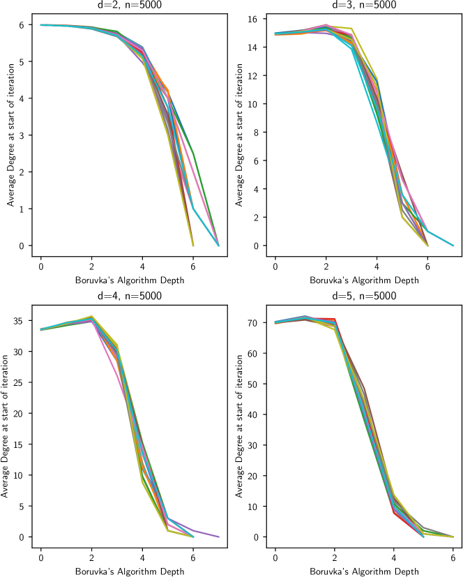
Figure 7.1: We randomly sample $20$ samples $P_{i},1\leq i\leq 20$ where $P_{i}\subseteq[0,1]^{d}$ and $\left|{P_{i}}\right|=5000$. We run Borůvka algorithm with $\mathcal{DT}\left({P_{i}}\right)$ as input for $d\in\{2,3,4,5\}$. In each iteration of Borůvka algorithm, we record the current average degree of the components, and plot the average degree progression for the $20$ different samples.

7.3 Adapting Borůvka to divide and conquer

The algorithm precomputes the graph $H=G_{\angle,\delta}\left({P}\right)$. Next, we turn Borůvka into a geometric divide and conquer algorithm. To this end, let $\mathsf{C}\subseteq[0,1]^{d}$ be some axis-parallel cube, and consider computing the MST of $P\cap\mathsf{C}$. Without any outside information, the output can only be a forest that is part of the final MST, and a set of candidate edges that might participate in the final MST. To this end, the algorithm splits $\mathsf{C}$ into $\nu=2^{d}$ identical subcells $\mathsf{C}_{1},\ldots,\mathsf{C}_{\nu}$.

The algorithm recursively computes the MST of $P_{i}=P\cap\mathsf{C}_{i}$, for all $i$. Specifically, the edges of the MST are edges of $H$, and as such, all the edges of the MST with exactly one endpoint in $P_{i}$ are in the cut $\Gamma(P_{i})=\left\{uv\in E\left({H}\right)\;\middle|\;u\in P_{i},v\in P\setminus P_{i}\right\}$. Intuitively, the size of this cut is quite small (roughly) $O(n^{1-1/d})$, and we can identify the vertices in $P_{i}$ adjacent to such edges. These vertices are portals, the set of all portals in $P_{i}$ is denoted by $\partial\left({P_{i}}\right)$.

Borůvka’s algorithm with portals.

Imagine running Borůvka only on the points of $P_{i}$. In every round, each connected component (in the current spanning forest) chooses the shortest edge in the cut it defines, and add it to the constructed forest. The catch is that if a connected component contains a portal point, then it might be part of a larger tree (in the larger forest) that is outside $P_{i}$. As such, this cut is no longer well defined (as it involves vertices and edges outside $P_{i}$). Thus, a connected component that contains a portal is frozen – it can no longer choose edges to add to the spanning tree. During a Borůvka round, all the components that are active (i.e., not frozen), each chooses the shortest edge in the cut they induce – note, that an active component might choose an edge connected to a frozen component. Thus, a frozen component might grow by active components attaching themselves to it. The algorithm continue doing rounds till all components are frozen.

A natural implementation of Borůvka is via collapsing each tree in the forest being constructed into a single node, and among parallel edges with the same endpoints, preserving the cheapest edge of the bunch. Thus, the execution on the modified Borůvka on $P_{i}$ results in an induced graph $G_{i}$ over $\partial\left({P_{i}}\right)$ – where the surviving edges are potential edges for use by the MST later on.

Pruning.

The number of edges of $G_{i}$ is potentially too large. The algorithm computes the MST of $G_{i}$ (treating it as its own graph, ignoring portals) running the standard Borůvka algorithm on $G_{i}$. The algorithm deletes from $G_{i}$ all the edges that do not appear in the computed MST.

To recap – every vertex of $G_{i}$ is a collapsed tree forming part of the final MST. All the edges of $G_{i}$ are candidate edges that might appear in the final MST– all these edges form a spanning tree of $G_{i}$. See Figure 7.2 and Figure 7.3 for a toy dry run on the Borůvka step and the pruning step.

(a)	(b)	(c)
(d)	(e)	(f)

Figure 7.2: (a) shows the axis parallel cube (in blue) and the points inside that we restrict ourselves to. $(b)$ shows some of the edges of $G_{\angle,\delta}\left({P}\right)$ inside the cube. $(c)$ shows the portal vertices in red, and all other points in blue. $(d)$ shows the connected components initially for Borůvka algorithm. $(e)$ shows the edges in cyan that were added by restricted Borůvka to EMST of $P$ in the first round. (f) Shows the new components after round one of Borůvka algorithm (note the previous blue vertex is now red because it joined a component with a portal). See Figure 7.3 for the rest.

(g)	(h)	(i)
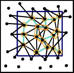
(j)	(k)

Figure 7.3: (g) again shows the new edges added to EMST in the second round of Borůvka. $(i)$ shows the final connected components since all components have a portal. $(j)$ shows the edges of the minimum spanning tree of the components which might be in the EMST of $P$. $(k)$ shows the final graph returned by the restricted Borůvka algorithm.

The conquer stage.

The algorithm recursively computes the (collapsed) graphs $G_{1},\ldots,G_{\nu}$, for $i=1,\ldots,\nu$. Next, the algorithm computes the set of portals $\partial=\partial\left({\mathsf{C}\cap P}\right)$, which is contained in $\cup_{i}\partial\left({P_{i}}\right)$. Let $E_{1}=\bigcup_{i<j}(P_{i},P_{j})$ be the set of all possible edges between the subproblems. Let $E_{2}=E_{1}\cap E\left({H}\right)$. Next, the algorithm computes the graph $G_{\mathsf{C}}=\cup_{i}G_{i}\cup E_{2}$. The algorithm runs the modified Borůvka with portals, described above, on the graph $G_{\mathsf{C}}$, with $\partial$ being the set of portals (thus, all the vertices comping from the children are portals in their own subproblem, but some of them lose their portal status as they migrate to the parent subproblem).

The overall algorithm.

We apply the above algorithm to $[0,1]^{d}$ and $P$. Note that the root has no portals, so the output is a single tree which is the MST.

Some low level implementation details.

We throw the points into a uniform grid over $[0,1]^{d}$, with each cell having volume $\Theta(1/n)$. We construct the quadtree over this grid in the natural way. We register each edge of $H$ with the lowest node of the quadtree that contains both endpoints. This can be done in $O(1)$ time per edge using a data-structure for LCA queries in $O(1)$ time. Now, scanning the edges, each vertex can compute the level in the quadtree where it stops being a portal. The LCA operation can be replaced by computing the level of the grid that contains a segment – using the floor operation and bit operations, this can be done in $O(1)$ time, see [Har11]. The rest of the algorithm implementation is as described above.

7.4 Analysis of the new MST algorithm

Clearly, edges that are added to an active component are edges that are minimal in their respective cuts, and thus must appear in the final MST. The more mysterious step in the pruning stage – let $pq$ be an edge that was deleted by the pruning stage from $G_{i}$. Observe that there is a path $\pi$ between $p$ and $q$ in the graph of $G_{i}$ using edges that are shorter than $pq$. Namely, $pq$ is the longest edge in a cycle, and can not appear in the final MST.

7.4.1 Running time analysis

Lemma 7.5.

Let $\mathsf{C}$ be a quadtree cell of depth $i$. Then, the number of portals in $\mathsf{C}\cap P$ is bounded by $O((n/2^{id})^{1-1/d}\log^{2}n)$, with high probability. This also bounds the total number of edges in $H$ adjacent to these vertices.

Proof:

A point of $p\in\mathsf{C}$ that is in distance larger than $\delta$ from the boundary of $\mathsf{C}$ can not be a portal, since $H$ does not contain such long edges. The volume of the moat $\mathcal{M}_{\mathsf{C}}$ containing such points is bounded by the surface area of $\mathsf{C}$ multiplied by $\delta$. That is $\alpha=(2d\cdot/2^{id})\delta$. Each such moat point has with high probability $O(\log n)$ edges in $H$. It follows that the expected number of portal edges is $O(\alpha n)=O((n/2^{id})^{1-1/d}\log^{2}n)$, as long as $\alpha>(\log n)/n$, by Lemma 2.8,  

Lemma 7.6.

The above algorithm runs in $O(n)$ expected time.

Proof:

Let $\nu=2^{d}$, and $P_{1},\ldots,P_{\nu}$ be the points sent to the children of the root of the quadtree. Let $n_{i}^{\prime}=\left|{\partial\left({P_{i}}\right)}\right|$, for all $i$. By Lemma 7.5, $n_{i}=O(n^{1-1/d}\log^{2}n)$ with high probability, and this also bounds the number of edges these portals have. Note, that each $G_{i}$ has exactly $n_{i}^{\prime}-1$ edges. Thus, the graph created in the root has $\sum_{i}n_{i}$ vertices, and $O(2^{d}n^{1-1/d}\log^{2}n)$ edges. Running Borůvka algorithm on this graph takes $O(n^{1-1/d}\log^{3}n)$ time. We thus get the recurrence

$$T(n)=O(n^{1-1/d}\log^{3}n)+\sum_{i}T(n_{i}).$$

It is easy to verify that the solution to this recurrence is $O(n)$, as $\sum_{i}n_{i}=n$ and $n_{i}<n/2$ with high probability. (To convince yourself of this, consider the over-simplified recurrence $S(n)=O(n^{1-1/d})+2^{d}S(n/2^{d})$.)  

Remark 7.7.

Note that the linear time MST algorithm can also be extended to a linear time MST algorithm for graphs with small separators. In that case, the portals are the separator vertices in the separator hierarchy, and we run the restricted Borůvka bottom up on the separator decomposition tree.

7.5 The result

The details of the following results are described in Section 7.

Theorem 7.8.

For fixed constant $d$, the MST of $n$ uniformly and independently sampled points from $[0,1]^{d}$ can be computed, by the above algorithm, in $O(n)$ expected time.

8 Simple distance selection in $O(n^{4/3}\log^{2/3}n)$ time in $d=2$

The task.

The input is a set $P$ of $n$ points picked randomly in $[0,1]^{2}$. For two sets $X,Y$, let

$$X*Y=\left\{\bigl{\{}x,y\}\;\middle|\;x\in X,y\in Y,x\neq y\right\}$$

be the set of all unordered pairs in $X\times Y$. Let $\Pi=P*P$, and for a fixed radius $\lambda$, let $\Pi_{\leq r}=\left\{\{p,q\}\in\Pi\;\middle|\;\left\|pq\right\|\leq r\right\}$ be the number of all pairs in $P$ that are in distance at most $r$ from each other. The task at hand is to compute $\left|{\Pi_{\leq r}}\right|$.

Basic idea and some tools.

Let $\mathsf{K}$ be a uniform $\mathsf{N}\times\mathsf{N}$ grid $\mathsf{K}$, where $\mathsf{N}=\left\lceil{(n/\log n)^{1/3}}\right\rceil$. Let $P_{i,j}$ denote the points of $P$ that fall in the grid cell $\mathsf{C}_{i,j}=[i/\mathsf{N},(i+1)/\mathsf{N}]\times[j/\mathsf{N},(j+1)/\mathsf{N}]$. Let $\Delta=\mathrm{diam}\left({\mathsf{C}_{i,j}}\right)=\sqrt{2}/\mathsf{N}$ be the diameter of a grid cells. We assume here that $r>8\Delta$. The case for $r\leq 8\Delta$ can be handled simply by bruteforce search of a fine grid.

Let $\xi_{i,j}=\left|{\left\{pq\in\Pi_{\leq r}\;\middle|\;p\in P_{i,j}\right\}}\right|$. Observe that $\left|{\Pi_{\leq r}}\right|=\sum_{i,j}|\xi_{i,j}|/2$. Thus, we restrict our attention to computing the values of $\xi_{i,j}$, for all $i,j$. For a grid cell $\mathsf{C}\in\mathsf{K}$, consider the sets

$$\mathcalb{b}_{\mathsf{K}}\left({\mathsf{C}}\right)=\left\{\mathsf{D}\in\mathsf{K}\;\middle|\;\mathsf{D}\subseteq\mathcalb{b}\left({\overline{\mathsf{c}}\left({\mathsf{C}}\right),r-2\Delta}\right)\bigr{.}\right\}\quad\text{and}\quad\mathcal{B}_{\mathsf{K}}\left({\mathsf{C}}\right)=\left\{\mathsf{D}\in\mathsf{K}\;\middle|\;\mathsf{D}\cap\mathcalb{b}\left({\overline{\mathsf{c}}\left({\mathsf{C}}\right),r+2\Delta}\right)\neq\emptyset\bigr{.}\right\},$$

where $\overline{\mathsf{c}}\left({\mathsf{C}}\right)$ is the center of $\mathsf{C}$. All the grid cells of $\mathcalb{b}_{\mathsf{K}}\left({\mathsf{C}}\right)$ are contained in any disk of radius $r$ centered at a point of $\mathsf{C}$. Similarly, $\mathcal{B}_{\mathsf{K}}\left({\mathsf{C}}\right)$ is a super set of all the grid cells that cover any disk of radius $r$ centered at any point of $\mathsf{C}$.

Let $\alpha_{i,j}=\left|{(\mathcalb{b}_{\mathsf{K}}\left({\mathsf{C}_{i,j}}\right)\cap P)*P_{i,j}}\right|$ and $\beta_{i,j}=\left|{(\mathcal{B}_{\mathsf{K}}\left({\mathsf{C}_{i,j}}\right)\cap P)*P_{i,j}}\right|$. Observe that $\alpha_{i,j}\leq\xi_{i,j}\leq\beta_{i,j}$. The set $\mathsf{O}_{i,j}=\mathcal{B}_{\mathsf{K}}\left({\mathsf{C}_{i,j}}\right)\setminus\mathcalb{b}_{\mathsf{K}}\left({\mathsf{C}_{i,j}}\right)$ is formed by all the grid cells intersecting a ring with outer radius $r+2\Delta$ and inner radius $r-2\Delta$. Let $Q_{i,j}=(\cup\mathsf{O}_{i,j})\cap P_{i,j}$. Observe that $P_{i,j}$ and $Q_{i,j}$ are disjoint. Consider the set of pairs they induce $P_{i,j}*Q_{i,j}$, and let $\tau_{i,j}$ be the number of pairs in $P_{i,j}*Q_{i,j}$ of length at most $r$. We have that $\xi_{i,j}=\alpha_{i,j}+\tau_{i,j}$. Thus, the algorithm would compute the quantities $\alpha_{i,j}$ and $\tau_{i,j}$ for all $i,j$. The algorithm would then compute $\sum_{i,j}\xi_{i,j}/2$, which is the desired quantity.

Low level procedures.

In the following, we assume that $n_{i,j}=|P_{i,j}|=O(n/\mathsf{N}^{2})$.

Lemma 8.1.

After $O(n+\mathsf{N}^{2})$ preprocessing, given a query of numbers $i,j$, one can compute $\alpha_{i,j}$ in $O(\mathsf{N})$ time.

Proof:

The algorithm computes the grid $\mathsf{K}$, the subset of points in $P$ in each grid cell, and their number. The algorithm then preprocess the grid so that given an a contiguous range of cells in a row (of the grid), the algorithm can report the number of points in this range in $O(1)$ time. This can be done using prefix sums for each row of the grid.

The desired quantity is $\alpha_{i,j}=\left|{(\mathcalb{b}_{\mathsf{K}}\left({\mathsf{C}_{i,j}}\right)\cap P)*P_{i,j}}\right|=n_{i,j}\sum_{\mathsf{C}_{u,v}\in\mathcalb{b}_{\mathsf{K}}\left({\mathsf{C}_{i,j}}\right)}n_{u,v}-n_{i,j}^{2}+\binom{n_{i,j}}{2}$. The set $\mathcalb{b}_{\mathsf{K}}\left({\mathsf{C}}\right)$ in a row (of the grid) is just an contiguous box, and one can compute the number of points of $P$ inside this box in $O(1)$ time. Thus, computing $\sum_{\mathsf{C}_{u,v}\in\mathcalb{b}_{\mathsf{K}}\left({\mathsf{C}_{i,j}}\right)}n_{u,v}$ can be done in $O(\mathsf{N})$ time.  

Lemma 8.2.

After $O(n+\mathsf{N}^{2})$ preprocessing, given a query numbers $i,j$, one can compute the set $Q_{i,j}=(\cup\mathsf{O}_{i,j})\cap P_{i,j}$ in $O(n/\mathsf{N})$ time (this also bounds its size).

Proof:

The set $\mathsf{O}$ is a “ring” of the grid of with $4$, and thus $|\mathsf{O}_{i,j}|=O(\mathsf{N})$. In particular, the set $\mathsf{O}_{i,j}$ can be computed in $O(\mathsf{N})$ time. The set $Q_{i,j}$ is formed by collecting all the point sets $P_{i,j}$ for cells $\mathsf{C}_{i,j}\in\mathsf{O}_{i,j}$. By assumption, $|P_{i,j}|=O(n/\mathsf{N}^{2})$, which readily implies that $|Q_{i,j}|=O(\mathsf{N}\cdot n/\mathsf{N}^{2})=O(n/\mathsf{N})$  

Lemma 8.3.

Let $Q$ and $U$ be two disjoint point sets in the plane, with $|Q|<|U|$. Then one can compute the number of pairs of points in $Q*U$ that are in distance at most $r$ from each other in $O(|Q|^{2}+|U|\log|Q|)$ time.

Proof:

Let $\mathcal{D}$ be the set of disks of radius $r$ centered at the points of $Q$. Compute the arrangement $\mathop{\mathrm{\mathcal{A}}}=\mathop{\mathrm{\mathcal{A}}}\left({Q}\right)$, and compute for every face of $\mathop{\mathrm{\mathcal{A}}}$ how many disks of $\mathcal{D}$ contain it. Furthermore, preprocess this arrangement for point-location queries in logarithmic time. This is all standard, and can be done in $O(|Q|^{2})$ time [BCKO08]. Now compute for each point of $U$ how many points of $Q$ are in distance at most $r$ from it, by performing a point-location query in $\mathop{\mathrm{\mathcal{A}}}$, and returning the depth of the query point.  

Algorithm restated.

The algorithm computes $\alpha_{i,j},P_{i,j},Q_{i,j}$ for all $i,j$ using the above procedures. It then computes for all $i,j$, the quantity $\tau_{i,j}$ by using Lemma 8.3. The algorithm now computes directly $\sum_{i,j}(\alpha_{i,j}+\tau_{i,j})/2$ and return it as the desired quantity.

Analysis.

Lemma 8.4.

Assuming $\mathsf{N}=O(\sqrt{n}/\log n)$, with probability $\geq 1-1/n^{O(1)}$, each grid cell contains $O(n/\mathsf{N}^{2})$ points of the random point set $P$.

Proof:

Each grid cell in the grid, in expectation, has $n/\mathsf{N}^{2}=\Omega(\log^{2}n)$ points of $P$ in it. Now using Chernoff’s inequality it follows that this quantity is concentrated (say up to $1\pm 1/2$ around its expectation) with probability $\geq 1-1/n^{O(1)}$. Using the union bound on the $\mathsf{N}^{2}$ grid cells, imply the claim.  

Running time analysis.

Computing the sets $Q_{i,j}$, for all $i,j\in\left\llbracket\mathsf{N}\right\rrbracket$, takes $O(n\mathsf{N})$ time, using Lemma 8.2. Computing $\tau_{i,j}$, using Lemma 8.3, takes

$$O(|P_{i,j}|^{2}+|Q_{i,j}|\log|P_{i,j}|)=O\left({(n/\mathsf{N}^{2})^{2}+(n/\mathsf{N})\log n}\right)$$

time. doing this for all $i,j\in\left\llbracket\mathsf{N}\right\rrbracket$ takes $O\left({n^{2}/\mathsf{N}^{2}+n\mathsf{N}\log n}\right)$ time. Clearly, this dominates the running time. Solving for $n^{2}/\mathsf{N}^{2}=n\mathsf{N}\log n$, we get $\mathsf{N}=(n/\log n)^{1/3}$. Clearly, the last step dominates the overall running time, which is $o(n\mathsf{N}\log n)=O(n^{4/3}\log^{2/3}n)$.

Theorem 8.5.

Let $P$ be a set of $n$ points picked uniformly and independently from $[0,1]^{2}$, and let $r$ be a parameter. One can compute, using the algorithm described above, the number of pairs of points in $P$ in distance $\leq r$ from each other, in $O(n^{4/3}\log^{2/3}n)$ time. The result returned by the algorithm is always correct, and the bound on the running time holds with probability $\geq 1-1/n^{O(1)}$.

9 Conclusions

To get Borůvka’s algorithm to run in $O(n)$ time for MST, we had to restrict its growth phase in each recursive call. This feels unnatural in many ways since it is intentionally slowing down the algorithm’s progress, but is necessary for a complete analysis. It remains open whether there is a method of showing Borůvka algorithm takes linear time in three or higher dimensions on random points. One possible direction would be to show that the average degree of the connected components in $G_{\angle,\delta}\left({P}\right)$, see Definition 7.2, increases (for $d\geq 3$) extremely slowly compared to the halving of connected components. This is an observation the authors noted in numerical simulations, yet were unable to prove. See Figure 7.1. If the average degree increase in every round of Borůvka’s algorithm can be bounded to a multiplicative constant $\xi<2$ in each round then that would imply that Borůvka’s algorithm runs in linear time.

References

- [AS00] Noga Alon and Joel H. Spencer “The Probabilistic Method, Second Edition” John Wiley, 2000 DOI: 10.1002/0471722154
- [BCKO08] Mark Berg, Otfried Cheong, Marc J. Kreveld and Mark H. Overmars “Computational Geometry: Algorithms and Applications” Santa Clara, CA, USA: Springer, 2008 DOI: 10.1007/978-3-540-77974-2
- [BKST78] J.. Bentley, H.. Kung, M. Schkolnick and C.. Thompson “On the average number of maxima in a set of vectors and applications” In J. Assoc. Comput. Mach. 25, 1978, pp. 536–543 DOI: 10.1145/322092.322095
- [Cal10] P. Calka “Tessellations” In New Perspectives in Stochastic Geometry London, England: Oxford University Press, 2010, pp. 606
- [Cha00] Bernard Chazelle “A minimum spanning tree algorithm with Inverse-Ackermann type complexity” In J. ACM 47.6, 2000, pp. 1028–1047 DOI: 10.1145/355541.355562
- [Cha01] Timothy M. Chan “On Enumerating and Selecting Distances” In Int. J. Comput. Geom. Appl. 11.3, 2001, pp. 291–304 DOI: 10.1142/S0218195901000511
- [Cha93] Bernard Chazelle “An optimal convex hull algorithm in any fixed dimension” In Discrete & Computational Geometry 10.4 Springer ScienceBusiness Media LLC, 1993, pp. 377–409 DOI: 10.1007/bf02573985
- [CHR16] Hsien-Chih Chang, Sariel Har-Peled and Benjamin Raichel “From Proximity to Utility: A Voronoi Partition of Pareto Optima” In Discrete Comput. Geom. 56.3, 2016, pp. 631–656 DOI: 10.1007/s00454-016-9808-0
- [CZ21] Timothy M. Chan and Da Wei Zheng “Hopcroft’s Problem, Log-Star Shaving, 2D Fractional Cascading, and Decision Trees” In CoRR abs/2111.03744, 2021 arXiv: https://arxiv.org/abs/2111.03744
- [DGL96] Luc Devroye, László Györfi and Gábor Lugosi “A Probabilistic Theory of Pattern Recognition” In A probabilistic theory of pattern recognition New York: Springer, 1996, pp. 67 DOI: 10.1007/978-1-4612-0711-5
- [Dwy88] Rex A. Dwyer “On the convex hull of random points in a polytope” In Journal of Applied Probability 25.4 Cambridge University Press (CUP), 1988, pp. 688–699 DOI: 10.2307/3214289
- [Dwy91] Rex A. Dwyer “Higher-dimensional Voronoi diagrams in linear expected time” In Discrete Comput. Geom. 6.3 Springer ScienceBusiness Media LLC, 1991, pp. 343–367 DOI: 10.1007/bf02574694
- [GLM22] P. Gillibert, T. Lachmann and C. Müllner “The VC-dimension of axis-parallel boxes on the Torus” In J. Complexity 68, 2022, pp. 101600 DOI: https://doi.org/10.1016/j.jco.2021.101600
- [Hag09] Torben Hagerup “An Even Simpler Linear-Time Algorithm for Verifying Minimum Spanning Trees” In 35th Int. Work. Graph-Theo. Concepts Comp. Sci. 5911, Lect. Notes in Comp. Sci., 2009, pp. 178–189 DOI: 10.1007/978-3-642-11409-0“˙16
- [Har11] S. Har-Peled “Geometric Approximation Algorithms” 173, Math. Surveys & Monographs Boston, MA, USA: Amer. Math. Soc., 2011 DOI: 10.1090/surv/173
- [Har11a] S. Har-Peled “On the Expected Complexity of Random Convex Hulls” In CoRR abs/1111.5340, 2011 URL: https://arxiv.org/abs/1111.5340
- [HJ20] Sariel Har-Peled and Mitchell Jones “On Separating Points by Lines” In Discret. Comput. Geom. 63.3, 2020, pp. 705–730 DOI: 10.1007/s00454-019-00103-z
- [HR15] Sariel Har-Peled and Benjamin Raichel “Net and Prune: A Linear Time Algorithm for Euclidean Distance Problems” In J. Assoc. Comput. Mach. 62.6 New York, NY, USA: ACM, 2015, pp. 44:1–44:35 DOI: 10.1145/2831230
- [HW87] D. Haussler and E. Welzl “-nets and simplex range queries” In Discrete Comput. Geom. 2, 1987, pp. 127–151 DOI: 10.1007/BF02187876
- [KKT95] David R. Karger, Philip N. Klein and Robert E. Tarjan “A Randomized Linear-Time Algorithm to Find Minimum Spanning Trees” In J. Assoc. Comput. Mach. 42.2 New York, NY, USA: Assoc. Comput. Mach., 1995, pp. 321–328 DOI: 10.1145/201019.201022
- [Kut02] Samuel Kutin “Extensions to McDiarmid’s inequality when differences are bounded with high probability”, 2002 URL: https://newtraell.cs.uchicago.edu/research/publications/techreports/TR-2002-04
- [Mar04] Martin Mareš “Two linear time algorithms for MST on minor closed graph classes” In Archivum Mathematicum 040.3 Department of Mathematics, Faculty of Science of Masaryk University, Brno, 2004, pp. 315–320 URL: http://eudml.org/doc/249321
- [Mul94] Ketan Mulmuley “Computational Geometry: An Introduction Through Randomized Algorithms” Englewood Cliffs, NJ: Prentice Hall, 1994 URL: http://www.amazon.com/Computational-Geometry-Introduction-Randomized-Algorithms/dp/0133363635
- [PR02] Seth Pettie and Vijaya Ramachandran “An optimal minimum spanning tree algorithm” In J. ACM 49.1, 2002, pp. 16–34 DOI: 10.1145/505241.505243
- [Ray70] H. Raynaud “Sur l’enveloppe convex des nuages de points aleatoires dans ” In J. Appl. Probab. 7, 1970, pp. 35–48
- [San53] L. Santalo “Introduction to Integral Geometry” Paris, Hermann, 1953
- [SW10] R. Schneider and W. Weil “Classical stochastic geometry” In New Perspectives in Stochastic Geometry London, England: Oxford University Press, 2010, pp. 606
- [VC13] V.. Vapnik and A.. Chervonenkis “On the Uniform Convergence of the Frequencies of Occurrence of Events to Their Probabilities” In Empirical Inference: Festschrift in Honor of Vladimir N. Vapnik Berlin, Heidelberg: Springer Berlin Heidelberg, 2013, pp. 7–12 DOI: 10.1007/978-3-642-41136-6˙2
- [VC71] V.. Vapnik and A.. Chervonenkis “On the uniform convergence of relative frequencies of events to their probabilities” In Theory Probab. Appl. 16, 1971, pp. 264–280
- [WW93] W. Weil and J.. Wieacker “Stochastic Geometry” In Handbook of Convex Geometry B North-Holland, 1993, pp. 1393–1438
- [Yao82] A.. Yao “On constructing minimum spanning trees in -dimensional spaces and related problems” In SIAM J. Comput. 11.4, 1982, pp. 721–736