Deep Maxout Network Gaussian Process

Abstract

Study of neural networks with infinite width is important for better understanding of the neural network in practical application. In this work, we derive the equivalence of the deep, infinite-width maxout network and the Gaussian process (GP) and characterize the maxout kernel with a compositional structure. Moreover, we build up the connection between our deep maxout network kernel and deep neural network kernels introduced in Lee et al. (2017). We also give an efficient numerical implementation of our kernel which can be adapted to any maxout rank. Numerical results show that doing Bayesian inference based on the deep maxout network kernel can lead to competitive results compared with their finite-width counterparts and deep neural network kernels introduced in Lee et al. (2017). This enlightens us that the maxout activation may also be incorporated into other infinite-width neural network structures such as the convolutional neural network (CNN).

Keywords Maxout Network $\cdot$ Gaussian Process  $\cdot$ Deep Learning

1 Introduction

Investigating neural networks with infinite width becomes a popular topic for two main reasons. First, neural networks in real application typically have a super large width, which may share similar properties with infinite-width neural networks ( Lee et al. (2019), Cao and Gu (2019)). Second, infinite-width neural networks have analytical properties which are easier to study (Yang et al. (2019)).

The infinite-width neural network as a GP was first derived in Neal (1996). Given a proper initialization, the output of a single-layer neural network becomes a GP with the kernel depending on the nonlinearity activation. In Lee et al. (2017)Matthews et al. (2018), the infinite-width deep neural network (DNN) as a GP was derived and the kernel has a compositional structure depending on the number of depth and the nonlinearity activation in the network. Moreover, they found that Bayesian inference with DNN kernels often outperforms their finite-width counterparts. Both Neal (1996) and Lee et al. (2017) studied neural networks with activations applied to single linear combinations of inputs. Following the infinite-width scheme, Novak et al. (2018) and Garriga-Alonso et al. (2018) developed the GP kernel based on the CNN structure and Yang (2019) developed the GP kernel based on neural structures such as the recurrent neural network (RNN), transformer, etc.

Although the deep maxout network is widely utilized in application, it has never been derived as a GP among previous works. The activation in maxout network applied on multiple linear combinations of inputs (or previous layers) so that the implementation in Neal (1996) and Lee et al. (2017) can not be directly applied here. In this work, we formally derive the deep, infinite-width maxout network as a GP and characterize its corresponding kernel as a compositional structure. Moreover, we give an efficient method based on numerical integration and interpolation to implement the kernel. We apply the deep maxtout network kernel to Bayesian inference on MNIST and CIFAR10 datasets and it can achieve encouraging results in numerical study.

1.1 Related Work

In early work, Neal (1996) derived that the single-layer, infinite-width neural network is a GP. With identical, independent distributions for the parameters initialization in each neuron, the hidden units are independent and identically distributed (i.i.d.), and the output of the network will converge to a GP by Central Limite Theorem (CLT). The covariance of the output corresponding to different inputs, which is the kernel of the GP, can be identified by the covariance of a single hidden unit, which is related to the type of the nonlinearity activation and initial variance levels of biases and weights.

Lee et al. (2017) discovered the equivalence between DNNs and GPs. They derived the equivalence by letting the width of each layer go to infinity sequentially. They also offered the derivation based on the Bayesian marginalization over intermediate layers, which did not depend on the order of limits but rely on Gaussian priors of parameters. The corresponding kernel of their deep neural network Gaussian Process (NNGP) then can be described in a compositional manner, that is, the covariance of the current layer is determined by that of the previous layer. They also proposed an efficient numerical implementation of the DNN GP kernel.

Novak et al. (2018) and Garriga-Alonso et al. (2018) studied the equivalence between CNNs with infinite channels and GPs. Novak et al. (2018) introduced a Monte Carlo method to compute CNN GP kernels. Garriga-Alonso et al. (2018) derived the same equivalence by letting the channels in each layer go to infinity sequentially as Lee et al. (2017) and calculated the kernel exactly for the infinite-channel CNN with the ReLU activation.

The neural network structures studied in Neal (1996), Lee et al. (2017) and Matthews et al. (2018) contain activations applied to single linear combinations of inputs (or outputs from the previous layer). In contrast, the activation in deep maxout networks applied to multiple linear combinations of inputs. Thus, directly applying previous derivations and the implementation of DNN kernels to the deep maxout network kernel is impossible.

1.2 Summary of Contributions

Our novel contributions in this work are as follows:

1. We derive the equivalence of deep, infinite-width maxout networks and GPs and detailedly characterize the corresponding GP kernel with a compositional structure. We further show that the deep maxout network kernel with maxout rank $q=2$ can be transformed to the DNN kernel with the ReLU activation with proper scale modification of the input and the variance level of initialization, which builds up the connection between the deep maxout network kernel and the deep neural network kernel.

2. We introduce an efficient implementation of the deep maxout network GP kernel based on numerical integration and interpolation method, which is with high precision and can be adapted to any maxout rank.

3. We conduct numerical experiments on MNIST and CIFAR10 datasets, showing that Bayesian inference with the deep maxtout network kernel often outperforms their finite-width counterparts and it can also achieve competitive results compared with DNN kernels in Lee et al. (2017), especially, in the more challenging dataset CIFAR10, which shows great potential to incorporate the maxout activation into other infinite-width neural network structures such as CNNs.

2 Review of the Maxout Network

The maxout network was initially introduced in Goodfellow et al. (2013). A maxout activation can be formalized as follows: given an input $\mathbb{x}\in\mathbb{R}^{d}$ ($\mathbb{x}$ may be the input vector or a hidden layer’s state), suppose the number of linear sub-units combined by a maxout activation (maxout rank) is $q$ (in general, $q\ll d$), a maxout activation first computes $q$ linear feature mappings $\mathbf{z}\in\mathbb{R}^{q}$, where

$$z_{i}=\mathbb{w}^{\top}_{i}\mathbb{x}+b_{i},\quad\mathbb{w}_{i}\in\mathbb{R}^{d},\quad i\in[q].$$ (1)

Afterwards, the output of the maxout hidden unit, $h_{maxout}$, is given as the maximum over the $q$ feature mappings:

$$h_{maxout}(\mathbb{x})=\text{max}\{z_{i}\}_{i=1}^{q}.$$ (2)

Thus, suppose $\mathbb{w}_{i}^{\prime}s$ are linearly independent, the maxout activation can be interpreted as performing a pooling operation over a $q$-dimensional affine space:

$$\mathcal{A}=\mathbb{b}+\mathcal{W},$$ (3)

where $\mathbb{b}$ is the bias vector and $\mathcal{W}=span(\{\mathbb{w}_{i}\}_{i=1}^{q})$, which is an affine transformation of the input space $\mathbb{R}^{d}$. The cross-channel max pooling activation selects the maximal output to be fed into the next layer. Such a special structure makes the maxout activation quite different from conventional activation units, which only work on an one-dimensional affine space.

For a fully-connected deep maxout network with L hidden layers, suppose the $l_{th}$ layer has $N_{l}$ hidden units with the maxout rank q, following previous notations, the output of the the $l_{th}$ layer $out^{l}$ would be

$$out^{l}=\{h^{l,j}_{maxout}(out^{l-1})\}_{j=1}^{N_{l-1}},$$ (4)

where the superscript $l,j$ of $h^{l,j}_{maxout}$ represents the $j_{th}$ maxout unit in the $l_{th}$ layer, and $h^{l,j}_{maxout}$ has the structure defined in (1) and (2) with (1) adapted to $out^{l-1}$:

$$z^{l,j}_{i}=(\mathbb{w}^{l,j}_{i})^{\top}\mathbb{x}+b^{l,j}_{i},\quad\mathbb{w}^{l,j}_{i}\in\mathbb{R}^{N_{l-1}},\quad i\in[q].$$ (5)

3 Deep Maxout Network with Infinite Width

3.1 Notation

Consider a fully connected maxout network with $L$ hidden layers, which are of width $N_{l}$ (for the $i_{th}$ layer). Let $d_{\text{in}}$ denote the input dimension, $d_{\text{out}}$ the output dimension, $\mathbb{x}\in\mathbb{R}^{d_{in}}$ the input vector and $\mathbb{z}\in\mathbb{R}^{d_{out}}$ the output of the network. For the $i_{th}$ unit in the $l_{th}$ hidden layer, let $x_{i}^{l}$ denote the return after the maxout activation and let $z_{i,j}^{l-1}$ denote the $j_{th}$ linear affine combination before the max-out activation. For the input layer, we let $x_{i}^{0}\equiv\mathbb{x}_{i}$ (the $i_{th}$ position of $\mathbb{x}$) so that we have $N_{0}=d_{in}$. And let $q$ denote the maxout rank of the activation. For the $i_{th}$ unit in the $l_{th}$ hidden layer, let $b_{i,j}^{l-1}$ denote the bias parameter of the $j_{th}$ sub-component of the $i_{th}$ unit, and $W_{i,j,k}^{l-1}$ the weight parameter of the corresponding $k_{th}$ position of the input. For the output layer, let $b_{i}^{L}$ denote the bias parameter of the $i_{th}$ output and $W_{i,k}^{L}$ denote the weight parameter of the corresponding $k_{th}$ position of the input. Suppose weight parameters are independently sampled from $N(0,\sigma_{w}^{2}/N_{l})$; bias parameters are independently sampled from $N(0,\sigma_{b}^{2})$, which are also independent from weight parameters. Let $\mathcal{GP}(\mu,K)$ denote a Gaussian process with mean and covariance functions $\mu(\cdot)$, $K(\cdot,\cdot)$, respectively. And we define function $F_{q}(\cdot)$ as

$$F_{q}(\rho) =E[max\{h_{1},...,h_{q}\}*max\{h_{1}^{\prime},...,h_{q}^{\prime}\}],~{}~{}~{}\text{for }\forall\rho\in[-1,1],$$ (6)

where $\{h_{i}\}_{i=1,..,q}\mathrel{\overset{i.i.d}{\scalebox{1.5}[1.0]{$\sim$}}}N(0,1)$, $\{h_{i}^{\prime}\}_{i=1,..,q}\mathrel{\overset{i.i.d}{\scalebox{1.5}[1.0]{$\sim$}}}N(0,1)$ and $Cor(h_{l},h_{m}^{\prime})=\mathbb{1}_{l=m}*\rho$.

Here $\mathbb{1}_{l=m}=\left\{\begin{aligned} 1&,&\text{if}~{}l=m\\ 0&,&l\neq m\end{aligned}\right.$

3.2 Deep, Infinite Width Maxout Networks as Gaussian Processes

We first derive the equvailence between GPs and infinite-width maxout networks in the single-layer case and then extend the equivalence to the multi-layer case.

3.2.1 Single-layer Maxout Networks as Gaussian Processes

The $i_{th}$ component of the network output of the input $\mathbb{x}$ is computed as

$$z_{i}(\mathbb{x}) =b_{i}^{1}+\sum_{k=1}^{N_{1}}W^{1}_{i,k}x_{k}^{1}(\mathbb{x})~{}~{}~{}~{}i=1,...,d_{out},$$ (7)

$$x_{k}^{1}(\mathbb{x}) =\max_{m\in[q]}(z^{0}_{k,m}(\mathbb{x})),$$

$$z^{0}_{k,m}(\mathbb{x}) =b_{k,m}^{0}+\sum_{r=1}^{d_{in}}W^{0}_{k,m,r}x_{r}.$$

Since weight parameters and bias parameters are all i.i.d. respectively, for the fixed input $\mathbb{x}$, $\{x_{k}^{1}(\mathbb{x})\}_{k=1,...,N_{1}}$ are i.i.d random variables. Let $\omega_{i,j,k}$ denote $W^{1}_{i,j,k}x_{k}^{1}(\mathbb{x})$, then, $\omega_{i,j,k}$, $k\in[N_{1}]$ are i.i.d, too. And we have

$$\mathbf{E}[\omega_{i,j,k}] =0,$$ (8)

$$Var(\omega_{i,j,k}) =\frac{\sigma_{w}^{2}\cdot\mathbf{E}[(x_{k}^{1}(\mathbb{x}))^{2})]}{N_{1}}.$$

By CLT,

$$\sum_{k=1}^{N_{1}}W^{1}_{i,j,k}x_{k}^{1}(\mathbb{x})\xrightarrow[N_{1}\rightarrow+\infty]{\mathcal{D}}N(0,\sigma_{w}^{2}\cdot\mathbf{E}[(x_{k}^{1}(\mathbb{x}))^{2}]).$$ (9)

By Continuous Mapping Theorem (CMT),

$$z_{i}(\mathbb{x})\xrightarrow[N_{1}\rightarrow+\infty]{\mathcal{D}}N(0,\sigma_{b}^{2}+\sigma_{w}^{2}\cdot\mathbf{E}[(x_{k}^{1}(\mathbb{x}))^{2})]).$$ (10)

Moreover, given a finite input set $\{\mathbb{x}^{\gamma_{1}},\cdots,\mathbb{x}^{\gamma_{n}}\}$, Let $\omega_{i,j,k}(r)$ denote $W^{1}_{i,j,k}x_{k}^{1}(\mathbb{x}^{\gamma_{r}})$, n-dimensional random vectors $\{\mathbb{v_{k}}=(\omega_{i,j,k}(1),\cdots,\omega_{i,j,k}(n))^{\top}\}_{k=1,...,N_{1}}$ are independent identically-distributed random vectors with mean 0, and covariance matrix $\Sigma(n)/N_{1}$, the $(i,j)_{th}$ element of $\Sigma(n)$, $\Sigma_{i,j}(n)=\sigma_{w}^{2}\cdot\mathbf{E}[x_{k}^{1}(\mathbb{x}^{\gamma_{i}})\cdot x_{k}^{1}(\mathbb{x}^{\gamma_{j}})]$. Therefore, combining the multi-dimensional CLT and CMT as above, we get

$$\begin{bmatrix}z_{i}(\mathbb{x}^{\gamma_{1}})\\ z_{i}(\mathbb{x}^{\gamma_{2}})\\ \vdots\\ z_{i}(\mathbb{x}^{\gamma_{n}})\end{bmatrix}\xrightarrow[N_{l}\rightarrow+\infty]{\mathcal{D}}N(0,\sigma_{b}^{2}*1_{n\times n}+\Sigma(n)),$$ (11)

where $1_{n\times n}$ is the $n\times n$ matrix whose elements are all 1, which is exactly the definition of a GP. We conclude that $z_{i}\sim\mathcal{GP}(0,K^{1})$, where

$$K^{1}(\mathbb{x},\mathbb{x}^{{}^{\prime}})=\mathbf{E}[z_{i}(\mathbb{x})z_{i}(\mathbb{x}^{{}^{\prime}})]=\sigma_{b}^{2}+\sigma_{w}^{2}\mathbf{E}[x_{k}^{1}(\mathbb{x})x_{k}^{1}(\mathbb{x}^{{}^{\prime}})]=\sigma_{b}^{2}+\sigma_{w}^{2}C(\mathbb{x},\mathbb{x}^{{}^{\prime}}),$$ (12)

where $C(\mathbb{x},\mathbb{x}^{{}^{\prime}})\equiv\mathbf{E}(x_{k}^{1}(\mathbb{x})\cdot x_{k}^{1}(\mathbb{x}^{\prime}))$. Note that $C(\mathbb{x},\mathbb{x}^{{}^{\prime}})$ is independent of $k$. Moreover, we have

$$\{z^{0}_{km}(\mathbb{x})\}~{}\mathrel{\overset{i.i.d}{\scalebox{1.5}[1.0]{$\sim$}}}~{}N(0,\sigma_{b}^{2}+\sigma_{w}^{2}\frac{||\mathbb{x}||^{2}}{d_{in}}),$$ (13)

$$\{z^{0}_{km}(\mathbb{x}^{\prime})\}~{}\mathrel{\overset{i.i.d}{\scalebox{1.5}[1.0]{$\sim$}}}~{}N(0,\sigma_{b}^{2}+\sigma_{w}^{2}\frac{||\mathbb{x}^{\prime}||^{2}}{d_{in}}),$$

$$Cov(z_{kl}^{0}(\mathbb{x}),~{}z_{km}^{0}(\mathbb{x}^{\prime}))=\mathbb{1}_{l=m}*(\sigma_{b}^{2}+\sigma_{w}^{2}\frac{<\mathbb{x},\mathbb{x}^{\prime}>}{d_{in}}),$$

where $<\mathbb{x},\mathbb{x}^{\prime}>$ is the Euclidean inner product of $\mathbb{x}$ and $\mathbb{x}^{\prime}$.

Then we have

$$C(\mathbb{x},\mathbb{x}^{\prime}) =E[x_{k}^{1}(\mathbb{x}),x_{k}^{1}(\mathbb{x}^{\prime})]$$ (14)

$$=E[max\{z_{k1}^{0}(\mathbb{x}),...,z_{kq}^{0}(\mathbb{x})\}*max\{z_{k1}^{0}(\mathbb{x}^{\prime}),...,z_{kq}^{0}(\mathbb{x}^{\prime})\}]$$

$$=\sqrt{\sigma_{b}^{2}+\sigma_{w}^{2}\frac{||\mathbb{x}||^{2}}{d_{in}}}*\sqrt{\sigma_{b}^{2}+\sigma_{w}^{2}\frac{||\mathbb{x}^{\prime}||^{2}}{d_{in}}}*F_{q}\bigg{(}\frac{\sigma_{b}^{2}+\sigma_{w}^{2}\frac{<\mathbb{x},\mathbb{x}^{\prime}>}{d_{in}}}{\sqrt{\sigma_{b}^{2}+\sigma_{w}^{2}\frac{||\mathbb{x}||^{2}}{d_{in}}}\sqrt{\sigma_{b}^{2}+\sigma_{w}^{2}\frac{||\mathbb{x}^{\prime}||^{2}}{d_{in}}}}\bigg{)}.$$

Note that, if we define

$$K^{0}(\mathbb{x},\mathbb{x}^{\prime})=\frac{<\mathbb{x},\mathbb{x}^{\prime}>}{d_{in}},$$ (15)

then we have

$$K^{1}(\mathbb{x},\mathbb{x}^{\prime})=\sigma_{b}^{2}+\sigma_{w}^{2}*\sqrt{\sigma_{b}^{2}+\sigma_{w}^{2}K^{0}(\mathbb{x},\mathbb{x})}*\sqrt{\sigma_{b}^{2}+\sigma_{w}^{2}K^{0}(\mathbb{x}^{\prime},\mathbb{x}^{\prime})}*F_{q}(\frac{\sigma_{b}^{2}+\sigma_{w}^{2}K^{0}(\mathbb{x},\mathbb{x}^{\prime})}{\sqrt{\sigma_{b}^{2}+\sigma_{w}^{2}K^{0}(\mathbb{x},\mathbb{x})}*\sqrt{\sigma_{b}^{2}+\sigma_{w}^{2}K^{0}(\mathbb{x}^{\prime},\mathbb{x}^{\prime})}}).$$ (16)

3.2.2 Multiple-layer Maxout Networks as Gaussian Processes

For a fully connected maxout network with $L$ hidden layers, the structure can be described as the following with a compositional manner.

For the output layer, the $i_{th}$ component, $z_{i}(x)$, can be computed by

$$z_{i}(\mathbb{x}) =b_{i}^{L}+\sum_{k=1}^{N_{L}}W_{i,k}^{L}x_{k}^{L}(\mathbb{x})$$ (17)

$$x_{k}^{L}(\mathbb{x}) =max(z_{k,m}^{L-1}(\mathbb{x}))$$

For the $l_{th}$ hidden layer, the $j_{th}$ linear affine combination in the $i_{th}$ unit, $z_{i,j}^{l}(x)$, can be computed by

$$z_{i,j}^{l}(\mathbb{x}) =b_{i,j}^{l}+\sum_{k=1}^{N_{1}}W^{l}_{i,j,k}x_{k}^{l}(\mathbb{x}),$$ (18)

$$x_{k}^{l}(\mathbb{x}) =\max_{m\in[q]}(z^{l-1}_{k,m}(\mathbb{x})),$$

for $l=0$,

$$z^{0}_{k,m}(\mathbb{x}) =b_{k,m}^{0}+\sum_{r=1}^{d_{in}}W^{0}_{k,m,r}x_{r}.$$ (19)

In analogy to the compositional structure in (16), for $\forall l\in\mathbb{N}_{+}$, we can define a compositional kernel as below:

$$K^{l}(\mathbb{x},\mathbb{x}^{\prime})=\sigma_{b}^{2}+\sigma_{w}^{2}*\sqrt{\sigma_{b}^{2}+\sigma_{w}^{2}K^{l-1}(\mathbb{x},\mathbb{x})}*\sqrt{\sigma_{b}^{2}+\sigma_{w}^{2}K^{l-1}(\mathbb{x}^{\prime},\mathbb{x}^{\prime})}*F_{q}(\frac{\sigma_{b}^{2}+\sigma_{w}^{2}K^{l-1}(\mathbb{x},\mathbb{x}^{\prime})}{\sqrt{\sigma_{b}^{2}+\sigma_{w}^{2}K^{l-1}(\mathbb{x},\mathbb{x})}*\sqrt{\sigma_{b}^{2}+\sigma_{w}^{2}K^{l-1}(\mathbb{x}^{\prime},\mathbb{x}^{\prime})}}),$$ (20)

where $K^{0}(\mathbb{x},\mathbb{x}^{\prime})$ is defined in (15).

The following theorem justifies the equavalence between infinite-width Multiple-layer Maxout Networks and GPs.

Theorem 1.

For a fully connected maxout network with $L$ hidden layers with the structure defined in (17), (18), (19), weights and biases intialized as described in 3.1, for any finite input set $\{\mathbb{x}^{\gamma_{j}}\}_{j=1}^{B}$, the distribution of the output $\{z_{i}(\mathbb{x}^{\gamma_{j}})\}_{j=1}^{B}$ will be a $\mathcal{GP}(0,K^{L})$, if $N_{1}\to\infty,...,N_{L}\to\infty$, where the kernel $K^{L}$ is defined as (20).

The proof of Theorem 1 is in A.1.

3.2.3 Bayesian Inference of Infinite-width, Deep Maxout Networks Using Gaussian Process Priors

With the deep maxout network gaussian process (MNNGP) defined above, we can apply the Bayesian inference to make predictions for testing data. Suppose that we have $B_{1}$ training data $X_{train}=\{\mathbb{x}^{\gamma_{j}}\}_{j=1}^{B_{1}}$, $Y_{train}=\{y^{\gamma_{j}}\}_{j=1}^{B_{1}}$ and $B_{2}$ testing data $X_{test}=\{\mathbb{x}^{\eta_{j}}\}_{j=1}^{B_{2}}$, the true outcome are $t_{train}=\{t^{\gamma_{j}}\}_{j=1}^{B_{1}}$ and $t_{test}=\{t^{\eta_{j}}\}_{j=1}^{B_{2}}$. In the Bayesian training, we assume that

$$y^{\gamma_{j}} =t^{\gamma_{j}}+\epsilon^{\gamma_{j}},$$ (21)

$$\begin{pmatrix}t_{train}\\ t_{test}\end{pmatrix} \sim N\bigg{(}0_{B_{1}+B_{2}},\begin{pmatrix}K_{X_{train},X_{train}}&K_{X_{test},X_{train}}\\ K_{X_{train},X_{test}}&K_{X_{test},X_{test}}\end{pmatrix}\bigg{)},$$

where $\epsilon^{\gamma_{j}}\mathrel{\overset{i.i.d}{\scalebox{1.5}[1.0]{$\sim$}}}N(0,\sigma_{\epsilon}^{2})$, $K_{X_{train},X_{train}}\in\mathbb{R}^{B_{1}\times B_{1}}$, $K_{X_{test},X_{train}}=K_{X_{train},X_{test}}^{T}\in\mathbb{R}^{B_{1}\times B_{2}}$ and $K_{X_{test},X_{test}}\in\mathbb{R}^{B_{2}\times B_{2}}$. Following the derivation in Lee et al. (2017), we have $t_{test}|X_{train},Y_{train}\sim N(\mu,\Sigma)$, where

$$\mu =K_{X_{test},X_{train}}(K_{X_{train},X_{train}}+\sigma_{\epsilon}^{2}I_{n})^{-1}t_{train},$$ (22)

$$\Sigma =K_{X_{test},X_{test}}-K_{X_{test},X_{train}}(K_{X_{train},X_{train}}+\sigma_{\epsilon}^{2})^{-1}K_{X_{train},X_{test}}.$$

3.3 Relation to DNN Kernel with ReLU Activation

DNNs with the ReLU activation is a speical case of deep maxout networks. We can also easily rewrite a maxout network with the maxout rank q = 2 into a DNN with the ReLU activation. So, for q = 2, in the finite-width regime, deep maxout networks and DNNs with the ReLU activation can be transformed to each other easily. Interestingly, we can derive that our deep maxout network kernel with the maxout rank equals to 2 (also with proper initialization and proper input scaling) is equivalent to the DNN Kernel with the ReLU activation defined in Lee et al. (2017), which is summariezd in the following proposition.

Proposition 1.

Let $K^{l}_{RL}(\mathbb{x},\mathbb{x^{\prime}};\tilde{\sigma}_{b},\tilde{\sigma}_{w})$ denote covariance functions of the infinite-width, $L-$layer Deep neural network with the ReLu activation defined in (Lee et al., 2017, Section 2) with bias parameter $\tilde{\sigma}_{b}$ and weight parameter $\tilde{\sigma}_{w}$, let $\sigma_{b}=\tilde{\sigma}_{b}$, $\sigma_{w}=\frac{\tilde{\sigma}_{w}}{\sqrt{2}}$, then for covariance functions $K^{l}(\mathbb{x},\mathbb{x^{\prime}})$ defined in (20), we have

$$K^{l}(\mathbb{x},\mathbb{x^{\prime}})=K^{l}_{RL}(\frac{\mathbb{x}}{\sqrt{2}},\frac{\mathbb{x}^{\prime}}{\sqrt{2}};\tilde{\sigma}_{b},\tilde{\sigma}_{w}),\text{ for }l\in\mathbb{N}_{+}.$$ (23)

The proof of Proposition 1 is in A.2.

From Proposition 1, we know that with proper initialization and proper scale of the input, the initial distribution of the output of the deep maxout network with maxout rank equals to 2 and the output of the deep neural network with the ReLU activation are the same if the width of hidden layers goes to infinity. That is, in the infinite-width regime, the initial output of the deep maxout network with $q=2$ and the deep neural network with the ReLU activation can also be transformed to each other, which implies the tight connection between deep maxout networks with $q=2$ and deep neural networks with the ReLU activation.

4 Implementation of Deep Maxout Network Kernel

To implement the deep maxout network kernel, it suffices to implement the function $F_{q}(\rho),~{}\rho\in[-1,1]$ efficiently. The idea of the implementation is that we first evaluate the values of $F_{q}(\cdot)$ for certain grids $\{\rho_{i}\}_{i=1,...,n_{\rho}}\subset[-1,1]$. Then, given any other $\rho^{*}\in[-1,1]$, $F_{q}(\rho^{*})$ will be evaluated by interpolation method based on the outputs from the grids. Our numerical implementation is easy to be adapted to any maxout rank $q$.

The details of evaluation of $F_{q}(\rho)$ for a specific $\rho\in[-1,1]$ are in B.

4.1 Numericial Implementation Example

Based on (38) in A.2, for the maxout rank $q=2$, we have, for $\forall\rho\in[-1,1]$

$$F_{2}(\rho)=2*E[max\{0,k_{1}\}*max\{0,k_{2}\}],$$ (24)

where $\begin{pmatrix}k_{1}\\ k_{2}\end{pmatrix}\sim N_{2}\bigg{(}0,\begin{pmatrix}1&\rho\\ \rho&1\end{pmatrix}\bigg{)}$. From Cho and Saul (2009), we have

$$E[max\{0,k_{1}\}*max\{0,k_{2}\}]=\frac{1}{2\pi}*(\sin(\arccos(\rho))+(\pi-\arccos(\rho))*\rho).$$ (25)

We compare numerical evaluations and theoretical values for $F_{2}(\rho)$ in Figure 1.

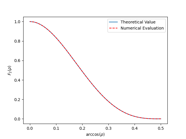
Figure 1: Theoretical Values VS Numerical Evaluations of $F_{2}(\rho)$. The plot shows a good match between the numerical implementation and theoretical values, which demonstrates the high precision of our numerical implementation.

5 Numerical Experiment

In the numerical experiment, we compare our results of the maxout neural network Gaussian process (MNNGP) with the results of the finite-width, deep maxout network on the MNIST and CIFAR10 datasets. We also compare our MNNGPs with NNGPs in Lee et al. (2017). Then we have a discussion about the effect of hyperparameters in MNNGPs. For MNNGPs, we formulate the classification problem as a regression task (Rifkin and Klautau (2004)). That is, class labels are encoded as a one-hot, zero-mean, regression target (i.e., entries of -0.1 for the incorrect class and 0.9 for the correct class). For training finite-width maxout networks, we will apply the mean square error (MSE) loss. The experiment setting of maxout networks with finite width can be found in C.1. And the setting of the Bayesian inference of MNNGPs can be founded in C.2.

5.1 Comparison with the Finite-width, Deep Maxout Network

Based on the experiment, no matter how large the maxout rank is, we can find that the Bayesian inference based on the MNNGP almost always outperforms their finite-width counterparts. Moreover, as the width of the maxout network gets larger, the performance of the finite-width, maxout network will be closer to that of the MNNGP. See Figure 2.

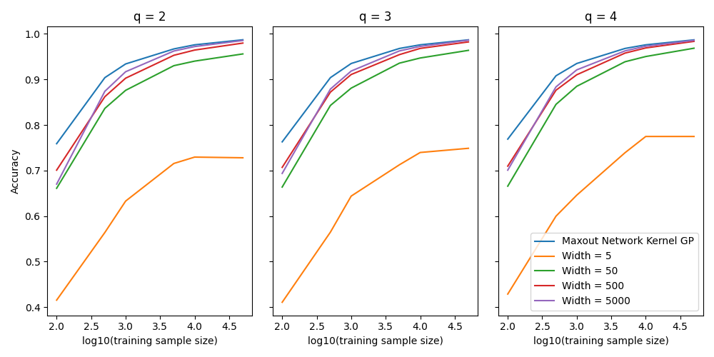
(a) Comparison with the finite-width, maxout network on MNIST

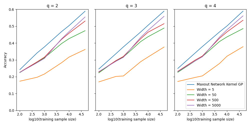
(b) Comparison with the finite-width, maxout network on CIFAR10

Figure 2: For each combination (number of training sample, maxout rank, network width), the test accuracy corresponding to the best set of hyperparameters searched by grid search (see C.1,C.2) is reported.

5.2 Comparison with NNGPs

We find that our MNNGP have competitive results compared with NNGPs with ReLU and Tanh kernels on MNIST and CIFAR10 datasets. Especially, our Deep Maxout Network Kernel always outperforms NNGPs in the more challenging dataset CIFAR10 with a significant improvement when the size of training set is large enough. See Table  1.

Table 1: The MNNGP often outperforms NNGPs with ReLU and Tanh avtivations from the view of test accuracies on MNIST and CIFAR-10 datasets. The reported MNNGP and NNGP results correspond to the best-performing combinations of tuning parameters on the validation set. Best models for a given training set size are specified by (activation-depth-$\sigma_{b}^{2}$-$\sigma_{w}^{2}$) for NNGPs, (widthq–maxout rank–depth-$\sigma_{b}$-$\sigma_{w}$) for finite-width maxout networks and (q-depth-$\sigma_{b}^{2}$-$\sigma_{w}^{2}$) for MNNGPs. $n_{t}$ is the size of the training set and $n_{v}$ is the size of the validation set.

Dataset $n_{t}$ $n_{v}$ Model Test accuracy MNIST 100 10K ReLU-100-0.83-1.79 0.7735 Tanh-100-0.97-3.14 0.7736 500-3-13-0.1-0.001 0.7070 4-9-1.17-3.48 0.7691 500 ReLU-100-0.83-1.79 0.8995 Tanh-50-1.86-3.48 0.8277 5000-4-9-0.1-0.001 0.8837 4-5-0.07-4.83 0.9079 1K ReLU-20-0.28-1.45 0.9279 Tanh-20-0.62-1.96 0.9266 5000-4-21-0.1-0.001 0.9210 4-5-0.34-4.83 0.9350 5K ReLU-7-0.07-0.61 0.9692 Tanh-3-0.00-1.11 0.9693 5000-4-1-0.1-0.001 0.9626 4-17-0.62-0.78 0.9683 10K ReLU-7-0.07-0.61 0.9765 Tanh-2-0.28-1.62 0.9773 5000-4-5-0.1-0.001 0.9729 3-9-1.72-0.78 0.9763 50K ReLU-1-0.48-0.10 0.9875 Tanh-1-0.00-1.28 0.9879 5000-4-1-0.5-0.001 0.9859 2-5-1.72-1.45 0.9870

Dataset $n_{t}$ $n_{v}$ Model Test accuracy CIFAR-10 100 5K ReLU-3-0.97-4.49 0.2673 Tanh-10-1.17-3.65 0.2718 500-3-21-0.1-0.001 0.2278 4-13-0.07-2.13 0.2487 500 ReLU-20-0.21-1.79 0.3395 Tanh-7-0.62-3.65 0.3291 500-3-21-0.1-0.001 0.2954 2-17-0.34-4.83 0.3410 1K ReLU-7-0.00-1.28 0.3608 Tanh-50-0.97-2.97 0.3702 5000-4-9-0.1-0.001 0.3185 4-17-0.07-4.16 0.3790 5K ReLU-3-1.03-4.66 0.4454 Tanh-10-0.38-3.65 0.4430 5000-4-9-0.1-0.001 0.4355 2-13-0.34-2.13 0.4677 10K ReLU-5-0.28-2.97 0.4780 Tanh-7-2.00-3.48 0.4766 5000-4-5-0.1-0.001 0.4783 3-21-0.07-1.45 0.5049 45K ReLU-3-1.86-3.31 0.5566 tanh-3-1.52-3.48 0.5558 5000-4-1-0.1-0.001 0.5611 4-13-0.34-4.16 0.5895

5.3 Discussion about the Effect of Hyperparameters

For the MNNGP model, there are four main hyperparameters, the maxout rank $q$, the depth, $\sigma_{w}^{2}$ and $\sigma_{b}^{2}$. For the maxout rank $q$, we can find that larger maxout rank $q$ can lead to better performance when the network is shallow, while there is no big difference when the network is deep (see the 1st, 3rd column in Figure3). For the depth, we can find that typically, larger depth can leads to better performance (see 1st, 2nd, 3rd row in Figure3). For $\sigma_{w}^{2}$ and $\sigma_{b}^{2}$, when the the network gets deep, small $\sigma_{w}^{2}$ may lead to ill-conditioned $K_{X_{train},X_{train}}$, so that computing $K_{X_{train},X_{train}}^{-1}$ fails and generate poor predictions (see $\sigma_{w}^{2}=0.1$ in 3rd column of Figure3). Generally, large $\sigma_{w}^{2}$ combined with moderate $\sigma_{b}^{2}$ can generate good performance.

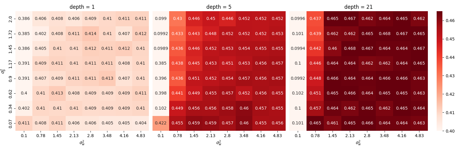
(a) Maxout Rank q = 2

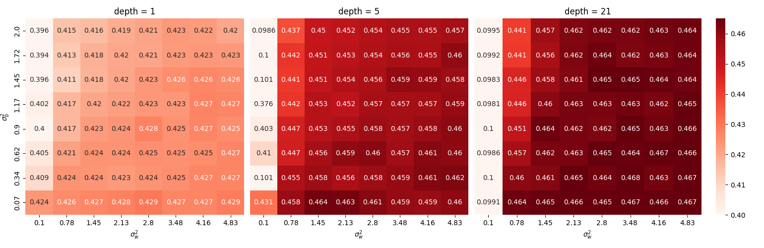
(b) Maxout Rank q = 3

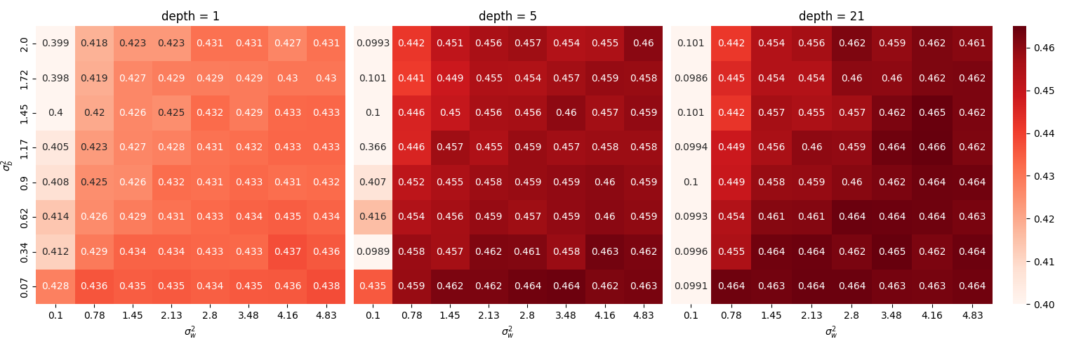
(c) Maxout Rank q = 4

Figure 3: The validation accuracy on CIFAR10 (see C.2) for the training sample size = 5000

6 Discussion

In this work, we derive the equivalence between the infinite-width, deep maxout network and the Gaussian process. The corresponding kernel is characterized by a compositional structure. One interesting discovery is that, with proper scale modification of the variance level of the initialization of biases and weights, as well as a proper scale of the input, the deep maxout network kernel with the maxout rank $q=2$ is the same as the deep neural network kernel with the ReLU activation, which demonstrates the equivalence of the initial outputs of the two networks in the infinite-width regime. Whether the output of the two infinite-width networks will still be the same in the training process is another interesting topic for the future work. To apply the deep maxout network kernel, we propose an implementation based on numerical integration and interpolation which is efficient, with high precision and easy to be adapted to any maxout rank. Experiments on MNIST and CIFAR10 datasets show that Bayesian inference with the deep maxout network kernel can lead to competitive results compared with their finite-width counterparts and the results in Lee et al. (2017), especially in the more challenging dataset, CIFAR10. Currently, many infinite-width neural structures only consider nonlinear activations applied to single linear combination of the input such as the ReLU and Tanh (see Novak et al. (2018), Garriga-Alonso et al. (2018) and Yang (2019)). We believe that incorporating the maxout activation into other infinite-width neural structures is promising to enhance the performances in practical application and this is left to future work.

Appendix A Technical Proofs

A.1 Proof of Theorem 1

Proof.

The derivation will based on the Bayesian marginalization over intermediate layers described in Lee et al. [2017].

Denote $X=\begin{pmatrix}\mathbb{x}^{\gamma_{1}}&\ldots&\mathbb{x}^{\gamma_{B}}\end{pmatrix}\in\mathbb{R}^{d_{in}\times B}$ and $Z_{i}=(z_{i}(\mathbb{x}^{\gamma_{1}}),...,z_{i}(\mathbb{x}^{\gamma_{B}}))^{T}\in\mathbb{R}^{B}$. We will study the distribution of $Z_{i}|X$.

For each layer $l$, denote the second moment matrix as below:

$$K_{i,j}^{l}=\left\{\begin{aligned} &\frac{1}{d_{in}}\sum_{m=1}^{d_{in}}x^{\gamma_{i}}_{m}x^{\gamma_{j}}_{m},&l=0\\ &\frac{1}{N_{l}}\sum_{m=1}^{N_{l}}x_{m}^{l}(\mathbb{x}^{\gamma_{i}})x_{m}^{l}(\mathbb{x}^{\gamma_{j}}),&l>0.\end{aligned}\right.$$ (26)

Note that since the weights and biases follow Gaussian distributions, we have $Z_{i}|K^{L}\sim N(0,G(K^{L}))$. From (17), (18), we know that $K^{l}$ only depend on $Z^{l-1}\equiv\{z_{m,b}^{l-1}(\mathbb{x}^{\gamma_{j}})\}$, where $Z^{l-1}$ denote the linear affine combinations before the max-out activation in $(l-1)_{th}$ layer. And the distribution of $Z^{l-1}$ only depend on $K^{l-1}$ from the definition. So we have

$$p(K^{l}|K^{l-1},K^{l-2},...,K^{0},X)=P(K^{l}|K^{l-1}).$$ (27)

Define function $F,G$ as below:

$$G(K^{l}) =\sigma_{w}^{2}K^{l}+\sigma_{b}^{2}\mathbb{1}\mathbb{1}^{T}\in\mathbb{R}^{B\times B},$$ (28)

$$H(K^{l}) \in\mathbb{R}^{B\times B},~{}where~{}~{}H(K^{l})_{i,j} =\sqrt{K^{l}_{i,i}}\sqrt{K^{l}_{j,j}}F_{q}(\frac{K^{l}_{i,j}}{\sqrt{K^{l}_{i,i}}\sqrt{K^{l}_{j,j}}}).$$

By the Law of Large Number (LLN), we could have for $l>0$,

$$\lim_{N_{l}\to\infty}p(K^{l}|K^{l-1})=\delta(K^{l}-H\circ G(K^{l-1})),~{}~{}~{}~{}~{}~{}~{}\delta(s)=\left\{\begin{aligned} 1&,&s=0\\ 0&,&s\neq 0.\end{aligned}\right.$$ (29)

For $l=0$, obviously, we have

$$p(K^{0}|X)=\delta(K^{0}-\frac{1}{d_{in}}X^{T}X).$$ (30)

Then we can write the $p(Z_{i}|X)$ as an integral over all the intermediate $K^{l}$, then we have

$$\lim_{N_{1}\to\infty,...,N_{L}\to\infty}p(Z_{i}|X) =\lim_{N_{1}\to\infty,...,N_{L}\to\infty}\int P(Z_{i}|K^{L})*(\prod_{l=1}^{L}p(K^{l}|K^{l-1}))*p(K^{0}|X)dK^{0}...dK^{L}$$ (31)

$$=\int p(Z_{i}|K^{L})*(\prod_{l=1}^{L}\delta(K^{l}-H\circ G(K^{l-1})))*\delta(K^{0}-\frac{1}{d_{in}}X^{T}X)dK^{0}...dK^{L}$$

$$=p(Z_{i}|K^{L}=(H\circ G)^{L}(K^{0})).$$

That is

$$\lim_{N_{1}\to\infty,...,N_{L}\to\infty}Z_{i}|X\sim N(0,G\circ(H\circ G)^{L}(K^{0})).$$ (32)

∎

A.2 Proof of Proposition 1

Proof.

We prove Proposition 1 by induction.

Let $F_{2}^{l}$ denote $F_{2}(\frac{\sigma_{b}^{2}+\sigma_{w}^{2}K^{l-1}(\mathbb{x},\mathbb{x}^{\prime})}{\sqrt{\sigma_{b}^{2}+\sigma_{w}^{2}K^{l-1}(\mathbb{x},\mathbb{x})}*\sqrt{\sigma_{b}^{2}+\sigma_{w}^{2}K^{l-1}(\mathbb{x}^{\prime},\mathbb{x}^{\prime})}})$ defined in (20).

STEP 1.

For $l=1$, eliminating subscript $k$ and superscript 0 in (7), we have

$$F_{2}^{1}=\frac{1}{\sqrt{\text{Var}z_{1}(x)\cdot\text{Var}z_{1}(x^{\prime})}}\mathbf{E}[\max(z_{1}(\mathbb{x}),z_{2}(\mathbb{x}))\cdot\max(z_{1}(\mathbb{x^{{}^{\prime}}}),z_{2}(\mathbb{x^{{}^{\prime}}}))].$$ (33)

Let $s,t,s^{{}^{\prime}},t^{{}^{\prime}}$ denote $\frac{z_{1}(\mathbb{x})}{\sqrt{\text{Var}z_{1}(x)}},\frac{z_{2}(\mathbb{x})}{\sqrt{\text{Var}z_{2}(x)}},\frac{z_{1}(\mathbb{x^{{}^{\prime}}})}{\sqrt{\text{Var}z_{1}(x^{\prime})}},\frac{z_{2}(\mathbb{x^{{}^{\prime}}})}{\sqrt{\text{Var}z_{2}(x^{\prime})}}$ in (33), respectively. By (13), we know

$$\begin{pmatrix}s\\ t\\ s^{\prime}\\ t^{\prime}\end{pmatrix} \sim N\begin{bmatrix}\begin{pmatrix}0\\ 0\\ 0\\ 0\end{pmatrix}\;,&\begin{pmatrix}1&0&\rho&0\\ 0&1&0&\rho\\ \rho&0&1&0\\ 0&\rho&0&1\end{pmatrix}\end{bmatrix},$$

where $\rho=\text{cor}{(z_{1}(x),z_{1}(x^{\prime}))}$. Then we have

$$\begin{aligned} F_{2}^{1}&=\mathbf{E}[\max(s,t)\cdot\max(s^{{}^{\prime}},t^{{}^{\prime}})]\\ &=\mathbf{E}[(\max(s-t,0)+t)\cdot(\max(s^{{}^{\prime}}-t^{{}^{\prime}},0)+t^{{}^{\prime}})]\\ &=\mathbf{E}[\max(s-t,0)\cdot\max(s^{{}^{\prime}}-t^{{}^{\prime}},0)]+\mathbf{E}[\max(s-t,0)\cdot t^{{}^{\prime}}]+\mathbf{E}[\max(s^{{}^{\prime}}-t^{{}^{\prime}},0)\cdot t]+\mathbf{E}[tt^{{}^{\prime}}]\\ &=\mathbf{E}[\max(s-t,0)\cdot\max(s^{{}^{\prime}}-t^{{}^{\prime}},0)]+2\mathbf{E}[\max(s-t,0)\cdot t^{{}^{\prime}}]+\mathbf{E}[tt^{{}^{\prime}}]\\ &=\underbrace{\mathbf{E}[\max(\nu,0)\cdot\max(\nu^{{}^{\prime}},0)]}_{\leavevmode\hbox to6.09pt{\vbox to6.09pt{\text{[drawing]}}}}+\underbrace{2\mathbf{E}[\max(s-t,0)\cdot t^{{}^{\prime}}]+\mathbf{E}[tt^{{}^{\prime}}]}_{\leavevmode\hbox to6.09pt{\vbox to6.09pt{\text{[drawing]}}}}\\ \end{aligned},$$ (34)

where

$$\begin{pmatrix}\nu\\ \nu^{\prime}\end{pmatrix} \sim N\begin{bmatrix}\begin{pmatrix}0\\ 0\\ \end{pmatrix}\;,&2\begin{pmatrix}1&\rho\\ \rho&1\\ \end{pmatrix}\end{bmatrix}.$$

Suppose we can show that $\leavevmode\hbox to8.53pt{\vbox to8.53pt{\text{[drawing]}}}=0$, then we have

$$K^{1}(\mathbb{x},\mathbb{x^{\prime}}) =\sigma_{b}^{2}+\sigma_{w}^{2}*\sqrt{\sigma_{b}^{2}+\sigma_{w}^{2}K^{0}(\mathbb{x},\mathbb{x})}*\sqrt{\sigma_{b}^{2}+\sigma_{w}^{2}K^{0}(\mathbb{x^{\prime}},\mathbb{x^{\prime}})}*\leavevmode\hbox to8.53pt{\vbox to8.53pt{\text{[drawing]}}}$$ (35)

$$=\tilde{\sigma}_{b}^{2}+\tilde{\sigma}_{w}^{2}*\sqrt{\frac{\text{Var}(z_{1}(x))\cdot\text{Var}(z_{1}(x^{\prime}))}{4}}*\leavevmode\hbox to8.53pt{\vbox to8.53pt{\text{[drawing]}}}$$

$$=\tilde{\sigma}_{b}^{2}+\tilde{\sigma}_{w}^{2}*\mathbf{E}[\max(z_{1}(x),0)\cdot\max(z_{1}(x),0)]$$

$$=K^{1}_{RL}(\frac{\mathbb{x}}{\sqrt{2}},\frac{\mathbb{x^{\prime}}}{\sqrt{2}};\tilde{\sigma}_{b},\tilde{\sigma}_{w}).$$

Now we show that = 0. Since $s$, $t$ and $t^{{}^{\prime}}$ are jointly normal, we have the following:

$$\mathbf{E}[\max(s-t,0)\cdot t^{\prime}] =\mathbf{E}_{s-t}[\mathbf{E}[\max(s-t,0)\cdot t^{\prime}|s-t]]$$ (36)

$$=\mathbf{E}_{s-t}[\max(s-t,0)\cdot\mathbf{E}[t^{\prime}|s-t]]$$

$$=-\frac{\rho}{2}\mathbf{E}_{s-t}[\max(s-t,0)\cdot(s-t)]$$

$$=-\frac{\rho}{2}\mathbf{E}_{s-t}[(\max(s-t,0))^{2}]$$

$$=-\frac{\rho}{2}.$$

Thus, we have $\leavevmode\hbox to8.53pt{\vbox to8.53pt{\text{[drawing]}}}=-\frac{\rho}{2}\cdot 2+\rho=0$.

STEP 2.

We suppose (23) holds for $l-1$, $l>1$, then for $l$

$$K^{l}(\mathbb{x},\mathbb{x}^{\prime}) =\sigma_{b}^{2}+\sigma_{w}^{2}*\sqrt{\sigma_{b}^{2}+\sigma_{w}^{2}K^{l-1}(\mathbb{x},\mathbb{x})}*\sqrt{\sigma_{b}^{2}+\sigma_{w}^{2}K^{l-1}(\mathbb{x}^{\prime},\mathbb{x}^{\prime})}*F_{q}^{l}$$ (37)

$$=\sigma_{b}^{2}+\sigma_{w}^{2}*\sqrt{\sigma_{b}^{2}+\sigma_{w}^{2}K^{l-1}(\mathbb{x},\mathbb{x})}*\sqrt{\sigma_{b}^{2}+\sigma_{w}^{2}K^{l-1}(\mathbb{x}^{\prime},\mathbb{x}^{\prime})}*\mathbf{E}[\max(s,t)\cdot\max(s^{{}^{\prime}},t^{{}^{\prime}})].$$

Similarly as in STEP 1.,

$$\begin{pmatrix}s\\ t\\ s^{\prime}\\ t^{\prime}\end{pmatrix} \sim N\begin{bmatrix}\begin{pmatrix}0\\ 0\\ 0\\ 0\end{pmatrix}\;,&\begin{pmatrix}1&0&\rho^{{}^{\prime}}&0\\ 0&1&0&\rho^{{}^{\prime}}\\ \rho^{{}^{\prime}}&0&1&0\\ 0&\rho^{{}^{\prime}}&0&1\end{pmatrix}\end{bmatrix},$$

where $\rho^{{}^{\prime}}=\frac{\sigma_{b}^{2}+\sigma_{w}^{2}K^{l-1}(\mathbb{x},\mathbb{x}^{\prime})}{\sqrt{\sigma_{b}^{2}+\sigma_{w}^{2}K^{l-1}(\mathbb{x},\mathbb{x})}*\sqrt{\sigma_{b}^{2}+\sigma_{w}^{2}K^{l-1}(\mathbb{x}^{\prime},\mathbb{x}^{\prime})}}$. Noticing that the previous trick does not depend on the value of $\rho$, we have

$$\mathbf{E}[\max(s,t)\cdot\max(s^{{}^{\prime}},t^{{}^{\prime}})]=\mathbf{E}[\max(\nu,0)\cdot\max(\nu^{{}^{\prime}},0)],$$ (38)

where

$$\begin{pmatrix}\nu\\ \nu^{\prime}\end{pmatrix} \sim N\begin{bmatrix}\begin{pmatrix}0\\ 0\\ \end{pmatrix}\;,&2\begin{pmatrix}1&\rho^{{}^{\prime}}\\ \rho^{{}^{\prime}}&1\\ \end{pmatrix}\end{bmatrix}.$$

Then, by the induction assumption, we have

$$K^{l}(\mathbb{x},\mathbb{x}^{\prime}) =\tilde{\sigma}_{b}^{2}+\tilde{\sigma}_{w}^{2}*\sqrt{\sigma_{b}^{2}+\sigma_{w}^{2}K^{l-1}(\mathbb{x},\mathbb{x})}*\sqrt{\sigma_{b}^{2}+\sigma_{w}^{2}K^{l-1}(\mathbb{x}^{\prime},\mathbb{x}^{\prime})}*\mathbf{E}[\max(\nu,0)\cdot\max(\nu^{{}^{\prime}},0)]$$ (39)

$$=\tilde{\sigma}_{b}^{2}+\tilde{\sigma}_{w}^{2}*\mathbf{E}_{z^{l-1}\sim\mathcal{GP}(0,K^{l-1}(x,x^{\prime}))}[\max(z^{l-1}(x),0)\cdot\max(\max(z^{l-1}(x^{{}^{\prime}}),0)]$$

$$=\tilde{\sigma}_{b}^{2}+\tilde{\sigma}_{w}^{2}*\mathbf{E}_{z^{l-1}\sim\mathcal{GP}(0,K^{l-1}(\frac{\mathbb{x}}{\sqrt{2}},\frac{\mathbb{x}^{\prime}}{\sqrt{2}};\tilde{\sigma}_{b}^{2},\tilde{\sigma}_{w}^{2}))}[\max(z^{l-1}(x),0)\cdot\max(\max(z^{l-1}(x^{{}^{\prime}}),0)$$

$$=K^{l}(\frac{x}{\sqrt{2}},\frac{x^{\prime}}{\sqrt{2}};\tilde{\sigma}_{b}^{2},\tilde{\sigma}_{w}^{2}).$$

Thus, (23) also holds for $l$ when it holds for $l-1$ . We finish the proof. ∎

Appendix B Evaluation of $F_{q}(\rho)$

Let $\phi(x)$ and $\Phi(x)$ denote the pdf and cdf of $N(0,1)$, respectively; $\phi_{2,\rho}(x,y)$ and $\Phi_{2,\rho}(x,y)$ denote the pdf and cdf of $N_{2}\bigg{(}0,\begin{pmatrix}1,\rho\\ \rho,1\end{pmatrix}\bigg{)}$. Let $R_{max}$ denote the maximum integration range and $n_{grid}$ the number of grid, then we take $n_{grid}\times n_{grid}$ points from the range $[-R_{max},R_{max}]\times[-R_{max},R_{max}]$, which are denoted by $\{(x_{i},y_{j})\}_{i,j=1,...,n_{grid}}$. $\phi(x)$, $\Phi(x)$, $\phi_{2,\rho}(x,y)$, and $\Phi_{2,\rho}(x,y)$ can be evaluated with function $scipy.stats.multivariate\_normal$[link] and $scipy.stats.norm$[link] in Python easily.

Here we first introduce how to evaluate $F_{q}(\rho)$ for the grids $\{\rho_{i}\}_{i=1,...,n_{\rho}}\subset[-1,1]$.

B.1 Evaluate $F_{q}(\rho)$ for $\rho\in(-1,1)$

Based on the definition in (LABEL:4), we denote $I=\arg\max_{i}\{h_{i}\}$ and $I^{\prime}=\arg\max_{i}\{h_{i}^{\prime}\}$. Then, we have

$$E[max\{h_{1},...,h_{q}\}*max\{h_{1}^{\prime},...,h_{q}^{\prime}\}] =E[max\{h_{1},...,h_{q}\}*max\{h_{1}^{\prime},...,h_{q}^{\prime}\}*\mathbb{1}_{I=I^{\prime}}]$$ (40)

$$~{}~{}~{}~{}+E[max\{h_{1},...,h_{q}\}*max\{h_{1}^{\prime},...,h_{q}^{\prime}\}*\mathbb{1}_{I\neq I^{\prime}}]$$

$$=q*E[max\{h_{1},...,h_{q}\}*max\{h_{1}^{\prime},...,h_{q}^{\prime}\}*\mathbb{1}_{I=I^{\prime}=1}]$$

$$~{}~{}~{}~{}+q*(q-1)E[max\{h_{1},...,h_{q}\}*max\{h_{1}^{\prime},...,h_{q}^{\prime}\}*\mathbb{1}_{I=1,I^{\prime}=2}].$$

Thus, we can focus on the evaluation of $E[max\{h_{1},...,h_{q}\}*max\{h_{1}^{\prime},...,h_{q}^{\prime}\}*\mathbb{1}_{I=I^{\prime}=1}]$ and $E[max\{h_{1},...,h_{q}\}*max\{h_{1}^{\prime},...,h_{q}^{\prime}\}*\mathbb{1}_{I=1,I^{\prime}=2}]$

B.1.1 Evaluate $E[max\{h_{1},...,h_{q}\}*max\{h_{1}^{\prime},...,h_{q}^{\prime}\}*\mathbb{1}_{I=I^{\prime}=1}]$

From the definition in (LABEL:4), we know that the set of pairs $\{(h_{i},h_{i}^{\prime})\}_{i=1,...,q}$ are i.i.d. random pairs with distribution $N_{2}\bigg{(}0,\begin{pmatrix}1,\rho\\ \rho,1\end{pmatrix}\bigg{)}$. Then we have

$$E[max\{h_{1},...,h_{q}\}*max\{h_{1}^{\prime},...,h_{q}^{\prime}\}*\mathbb{1}_{I=I^{\prime}=1}] =\int xy\phi_{2,\rho}(x,y)\Phi^{q-1}_{2,\rho}(x,y)dxdy.$$ (41)

Applying numerical integration. we have

$$\int xy\phi_{2,\rho}(x,y)\Phi^{q-1}_{2,\rho}(x,y)dxdy \approx\frac{\sum_{i,j=1}^{n_{grid}}x_{i}y_{j}\phi_{2,\rho}(x_{i},y_{j})\Phi^{q-1}_{2,\rho}(x_{i},y_{j})}{\sum_{i,j=1}^{n_{grid}}\phi_{2,\rho}(x_{i},y_{j})\Phi^{q-1}_{2,\rho}(x_{i},y_{j})}.$$ (42)

B.1.2 Evaluate $E[max\{h_{1},...,h_{q}\}*max\{h_{1}^{\prime},...,h_{q}^{\prime}\}*\mathbb{1}_{I=1,I^{\prime}=2}]$

From the definition in (LABEL:4), we have

$$(h_{1},h_{1}^{\prime},h_{2},h_{2}^{\prime}) \sim N_{4}\bigg{(}0,\begin{pmatrix}1&\rho&0&0\\ \rho&1&0&0\\ 0&0&1&\rho\\ 0&0&\rho&1\end{pmatrix}\bigg{)}.$$ (43)

Then, we have

$$(h_{1}^{\prime},h_{2})|(h_{1}=x,h_{2}^{\prime}=y)\sim N_{2}\bigg{(}\begin{pmatrix}\rho*x\\ \rho*y\end{pmatrix},\begin{pmatrix}1-\rho^{2}&0\\ 0&1-\rho^{2}\end{pmatrix}\bigg{)}.$$ (44)

So,

$$E[max\{h_{1},...,h_{q}\}*max\{h_{1}^{\prime},...,h_{q}^{\prime}\}*\mathbb{1}_{I=1,I^{\prime}=2}] =\int xy\phi(x)\phi(y)\Phi(\frac{(1-\rho)x}{\sqrt{1-\rho^{2}}})\Phi(\frac{(1-\rho)y}{\sqrt{1-\rho^{2}}})\Phi_{2,\rho}(x,y)dxdy.$$ (45)

Applying numerical integration, we have

$$\int xy\phi(x)\phi(y)\Phi(\frac{(1-\rho)x}{\sqrt{1-\rho^{2}}})\Phi(\frac{(1-\rho)y}{\sqrt{1-\rho^{2}}})\Phi^{q-2}_{2,\rho}(x,y)dxdy \approx\frac{\sum_{i,j=1}^{n_{grid}}x_{i}y_{j}\phi(x_{i})\phi(y_{j})\Phi(\frac{(1-\rho)x_{i}}{\sqrt{1-\rho^{2}}})\Phi(\frac{(1-\rho)y_{j}}{\sqrt{1-\rho^{2}}})\Phi_{2,\rho}^{q-2}(x_{i},y_{j})}{\sum_{i,j=1}^{n_{grid}}\phi(x_{i})\phi(y_{j})\Phi(\frac{(1-\rho)x_{i}}{\sqrt{1-\rho^{2}}})\Phi(\frac{(1-\rho)y_{j}}{\sqrt{1-\rho^{2}}})\Phi_{2,\rho}^{q-2}(x_{i},y_{j})}.$$ (46)

B.2 Evaluate $F_{q}(\rho)$ for $\rho=\pm 1$

For $\rho=1$, $h_{i}=h_{i}^{\prime}$ almost surely. Then, we have

$$E[max\{h_{1},...,h_{q}\}*max\{h_{1}^{\prime},...,h_{q}^{\prime}\}] =E[(max\{h_{1},...,h_{q}\})^{2}]$$ (47)

$$=q*\int x^{2}\phi(x)\Phi^{q-1}(x)dx$$

$$\approx q*\frac{\sum_{i=1}^{n_{grid}}x_{i}^{2}\phi(x_{i})\Phi^{q-1}(x_{i})}{\sum_{i=1}^{n_{grid}}\phi(x_{i})\Phi^{q-1}(x_{i})}.$$

For $\rho=-1$, $h_{i}=-h_{i}^{\prime}$ almost surely. Then, we have

$$E[max\{h_{1},...,h_{q}\}*max\{h_{1}^{\prime},...,h_{q}^{\prime}\}] =-E[(max\{h_{1},...,h_{q}\})*min\{h_{1},...,h_{q}\}]$$ (48)

$$=-q(q-1)*\int_{x>y}xy\phi(x)\phi(y)(\Phi(x)-\Phi(y))^{q-2}dxdy$$

$$\approx-q(q-1)\frac{\sum_{i=1}^{n_{grid}}x_{i}y_{j}\phi(x_{i})\phi(y_{j})*(\Phi(x_{i})-\Phi(y_{j}))^{q-2}*\mathbb{1}_{x_{i}>y_{j}}}{\sum_{i=1}^{n_{grid}}\phi(x_{i})\phi(y_{j})(\Phi(x_{i})-\Phi(y_{j}))^{q-2}*\mathbb{1}_{x_{i}>y_{j}}}.$$

Then, for $\forall\rho\in[-1,1]$, $F_{q}(\rho)$ will be evaluated by interpolation based on the grids.

B.3 Evaluation of $F_{q}(\rho)$ by Interpolation

For $\forall\rho\in[-1,1]$, let $\rho\in[\rho_{i},\rho_{i+1}]$, then, we have

$$F_{q}(\rho)=\frac{\rho_{i+1}-\rho}{\rho_{i+1}-\rho_{i}}*F_{q}(\rho_{i})+\frac{\rho-\rho_{i}}{\rho_{i+1}-\rho_{i}}*F_{q}(\rho_{i+1}).$$

Appendix C Details of Experiment Setup

C.1 Setup for the finite width, deep maxout network

Hyperparameters tuning

The learning rate of training finite-width, deep maxout networks is $10^{-5}$. The batch size is 256. The number of epochs is 200.

We apply grid search to tune other hyperparameters. We select the width from $\{5,50,500,5000\}$, maxout rank $q$ from $\{2,3,4\}$, depth from $\{1,5,9,13,17,21\}$, the standard deviation of the initialization of weights from $\{0.001,0.01,0.1,0.5,1\}$, the standard deviation of the initialization of biases from $\{0.1,0.5,1\}$.

For each choice of hyperparameters and for both MNIST and CIFAR-10 datasets, the validation results and testing results are generated the same as C.2.

C.2 Setup for the Bayesian inference based on MNNGP

Parameters of Lookup Tables

For all the experiments we use pre-computed lookup tables F with $n_{grid}$ = 501, $n_{\rho}$ = 1001, and $R_{max}$ = 100. The target noise $\sigma_{\epsilon}^{2}$ is set to $10^{-10}$ initially, and is increased by a factor of 10 when the Cholesky decomposition failed while solving (22).

Hyperparameters tuning

We select $q$ from $\{2,3,4\}$, depth from $\{1,5,9,13,17,21\}$, $\sigma_{b}^{2}$ from $\{\frac{2\cdot i}{29}|\;i\text{ mod }4=1,i\in[30]\}$ and $\sigma_{w}^{2}$ from $\{0.1+\frac{49\cdot i}{290}|\;i\text{ mod }4=0,i\in[30]\}$.

Validation Results Report

For both MNIST and CIFAR-10 datasets, we randomly shuffle the original training set first. Then the first $n_{t}$ samples from the shuffled training set are selected to be the training set and first $n_{v}$ samples from the remaining ones are treated as the validation sets. For each combination of hyperparameters, we estimate the model on the training set and calculate validation accuracy on the validation set. We repeat the previous procedure 20 times and choose the combination of hyperparameters with the highest mean accuracy.

Testing Results Report After selecting hyperparameters, we apply the previous data splitting procedure on the training set, estimate the model on the training set of size $n_{t}$ and calculate the testing accuracy on the original testing set. We repeat the procedure 20 times and report the mean testing accuracy.

References

- Lee et al. [2017] Jaehoon Lee, Yasaman Bahri, Roman Novak, Samuel S Schoenholz, Jeffrey Pennington, and Jascha Sohl-Dickstein. Deep neural networks as gaussian processes. arXiv preprint arXiv:1711.00165, 2017.
- Lee et al. [2019] Jaehoon Lee, Lechao Xiao, Samuel Schoenholz, Yasaman Bahri, Roman Novak, Jascha Sohl-Dickstein, and Jeffrey Pennington. Wide neural networks of any depth evolve as linear models under gradient descent. In H. Wallach, H. Larochelle, A. Beygelzimer, F. d'Alché-Buc, E. Fox, and R. Garnett, editors, Advances in Neural Information Processing Systems, volume 32. Curran Associates, Inc., 2019. URL https://proceedings.neurips.cc/paper/2019/file/0d1a9651497a38d8b1c3871c84528bd4-Paper.pdf.
- Cao and Gu [2019] Yuan Cao and Quanquan Gu. Generalization bounds of stochastic gradient descent for wide and deep neural networks. In H. Wallach, H. Larochelle, A. Beygelzimer, F. d'Alché-Buc, E. Fox, and R. Garnett, editors, Advances in Neural Information Processing Systems, volume 32. Curran Associates, Inc., 2019. URL https://proceedings.neurips.cc/paper/2019/file/cf9dc5e4e194fc21f397b4cac9cc3ae9-Paper.pdf.
- Yang et al. [2019] Greg Yang, Jeffrey Pennington, Vinay Rao, Jascha Sohl-Dickstein, and Samuel S. Schoenholz. A mean field theory of batch normalization. CoRR, abs/1902.08129, 2019. URL http://arxiv.org/abs/1902.08129.
- Neal [1996] Radford M Neal. Priors for infinite networks. In Bayesian Learning for Neural Networks, pages 29–53. Springer, 1996.
- Matthews et al. [2018] Alexander G de G Matthews, Mark Rowland, Jiri Hron, Richard E Turner, and Zoubin Ghahramani. Gaussian process behaviour in wide deep neural networks. arXiv preprint arXiv:1804.11271, 2018.
- Novak et al. [2018] Roman Novak, Lechao Xiao, Jaehoon Lee, Yasaman Bahri, Greg Yang, Jiri Hron, Daniel A Abolafia, Jeffrey Pennington, and Jascha Sohl-Dickstein. Bayesian deep convolutional networks with many channels are gaussian processes. arXiv preprint arXiv:1810.05148, 2018.
- Garriga-Alonso et al. [2018] Adrià Garriga-Alonso, Carl Edward Rasmussen, and Laurence Aitchison. Deep convolutional networks as shallow gaussian processes. arXiv preprint arXiv:1808.05587, 2018.
- Yang [2019] Greg Yang. Tensor programs I: wide feedforward or recurrent neural networks of any architecture are gaussian processes. CoRR, abs/1910.12478, 2019. URL http://arxiv.org/abs/1910.12478.
- Goodfellow et al. [2013] Ian Goodfellow, David Warde-Farley, Mehdi Mirza, Aaron Courville, and Yoshua Bengio. Maxout networks. In Proceedings of the 30th International Conference on Machine Learning, volume 28 of Proceedings of Machine Learning Research, pages 1319–1327, Atlanta, Georgia, USA, 17–19 Jun 2013. PMLR.
- Cho and Saul [2009] Youngmin Cho and Lawrence Saul. Kernel methods for deep learning. In Y. Bengio, D. Schuurmans, J. Lafferty, C. Williams, and A. Culotta, editors, Advances in Neural Information Processing Systems, volume 22. Curran Associates, Inc., 2009. URL https://proceedings.neurips.cc/paper/2009/file/5751ec3e9a4feab575962e78e006250d-Paper.pdf.
- Rifkin and Klautau [2004] Ryan Rifkin and Aldebaro Klautau. In defense of one-vs-all classification. The Journal of Machine Learning Research, 5:101–141, 2004.