Learning Properties of Simulation-Based Games

Computational and Data Requirements for Learning Generic Properties of Simulation-Based Games

Abstract

Empirical game-theoretic analysis (EGTA) is primarily focused on learning the equilibria of simulation-based games. Recent approaches have tackled this problem by learning a uniform approximation of the game’s utilities, and then applying precision-recall theorems: i.e., all equilibria of the true game are approximate equilibria in the estimated game, and vice-versa. In this work, we generalize this approach to all game properties that are well behaved (i.e., Lipschitz continuous in utilities), including regret (which defines Nash and correlated equilibria), adversarial values, and power-mean and Gini social welfare. Further, we introduce a novel algorithm—progressive sampling with pruning ($\operatorname{PSP}$)—for learning a uniform approximation and thus any well-behaved property of a game, which prunes strategy profiles once the corresponding players’ utilities are well-estimated, and we analyze its data and query complexities in terms of the a priori unknown utility variances. We experiment with our algorithm extensively, showing that 1) the number of queries that PSP saves is highly sensitive to the utility variance distribution, and 2) PSP consistently outperforms theoretical upper bounds, achieving significantly lower query complexities than natural baselines. We conclude with experiments that uncover some of the remaining difficulties with learning properties of simulation-based games, in spite of recent advances in statistical EGTA methodology, including those developed herein.

1 Introduction

Game theory is the standard conceptual framework used to analyze strategic interactions among rational agents in multiagent systems. Traditionally, a game theorist assumes access to a complete specification of a game, including any stochasticity in the environment. More recently, driven by high-impact applications, e.g., wireless spectrum (Gandhi et al., 2007; Weiss et al., 2017) and online advertisement auctions (Jordan and Wellman, 2010; Varian, 2007), researchers have turned their attention to analyzing games for which a complete specification is either too complex or too expensive to produce (Wellman, 2006). When such games are observable through simulation, they are called simulation-based games Vorobeychik and Wellman (2008). The literature on empirical game-theoretic analysis (EGTA) aims to analyze these games. This paper concerns statistical EGTA, in which the goal is to develop algorithms, ideally with finite-sample guarantees, that learn properties of games (e.g., their equilibria), even when a complete description of the game is not available.

In the statistical analysis of simulation-based games, it is generally assumed that the game analyst has access to an oracle, i.e., a simulator, that can produce agent utilities, given an arbitrary strategy profile and a random condition. This random condition can represent any number of exogenous random variables (e.g., the weather), and it can also incorporate an entropy source based on which any randomness within the game (e.g., the roll of a dice) is generated.

Randomness renders it necessary to query the simulator multiple times at each strategy profile to estimate the game’s utilities. This, in turn, necessitates that we sample many random conditions. To measure the amount of “work” needed to produce estimates within some specified error with high probability, we define two complexity measures. Data complexity is the requisite number of sampled random conditions, while query complexity is the requisite number of simulator queries. Data complexity is relevant in Bayesian games, such as private-value auctions. Doing market research (e.g., collecting data to learn about the bidders’ private values) can be expensive, but each of these expensive samples can then be used to query all strategy profiles. Query complexity is the more natural metric in computation-bound games, such as Starcraft Tavares et al. (2016), where simulating the game to determine utilities can be expensive, regardless of access to a random seed.

Prior work in EGTA has focused primarily on identifying a specific property of games, usually one or all equilibria. For example, Tuyls et al. (2020) show that if one can accurately estimate all the players’ utilities in a game, then one can also accurately estimate all equilibria. If one is willing to settle for a single equilibrium, more efficient algorithms can be employed (Fearnley et al., 2015; Wellman, 2006), and even when all equilibria are of interest, algorithms that prune strategy profiles, even heuristically (Areyan Viqueira et al., 2019, 2020), can potentially reduce the requisite amount of work. In this paper, we aim to broaden the scope of statistical EGTA beyond its primary focus on equilibria to arbitrary properties of games. In particular, we consider properties like welfare at various strategy profiles, as well as extreme properties (e.g., maximum or minimum welfare) and their witnesses (e.g., strategy profiles that realize maximum welfare).

We adopt the uniform approximation framework of Tuyls et al. (2020), wherein one game is an $\varepsilon$-approximation of another if players’ utilities differ by no more than $\varepsilon$ everywhere. Tuyls et al. (2020) show that an $\varepsilon$-uniform approximation of a game implies a $2\varepsilon$-uniform approximation of regret (i.e., equilibria). We extend this idea to approximate many such properties, by showing that Lipschitz continuity is a sufficient condition for a property (and its extrema) to be uniformly approximable. For example, both power-mean and Gini social welfare — two classes of welfare measures that capture utilitarian and egalitarian welfare — and their extrema, can be estimated using our framework. We also rederive known results about approximating equilibria (Areyan Viqueira et al., 2019; Tuyls et al., 2020) as special cases of our general theory, and we argue that our theory applies to equilibria of derived games, such as correlated equilibria, and to derived games themselves, such as team games.

Next, we develop a novel learning algorithm that estimates simulation-based games. We move beyond earlier work by Tuyls et al. (2020), who employed standard Hoeffding bounds for mean estimation, and follow Areyan Viqueira et al. (2020), who derive empirical variance-aware bounds: they bound each utility in terms of an empirical estimate of the largest variance across all utilities. We rederive their bounds, obtaining tighter constants; however, instead of uniform bounds, we present non-uniform, variance-sensitive bounds: we bound each utility in terms of its own (empirical) variance. Areyan Viqueira et al. employed their bounds to prune strategy profiles with provably high regret. We develop an algorithm that uses our bounds to prune based on an alternative criterion: profiles are pruned as soon as they are provably well estimated. Finally, we derive a sampling schedule that guarantees the correctness of our algorithm upon termination.

In addition to establishing its correctness, we also characterize the efficiency of our pruning algorithm. We argue that our algorithm is nearly optimal with respect to both data and query complexities. It can thus be used to learn myriad game properties, like welfare and regret, with complexity dependent on the size of the game, without requiring any a priori information about the players’ utilities beyond their ranges; even variances need not be known a priori.

We also experiment extensively with our algorithm and a variety of natural baselines on a suite of games generated using GAMUT Nudelman et al. (2004), enhanced with various noise structures so that they mimic simulation-based games. Our findings can be summarized as follows:

• We show that the number of queries our pruning algorithm requires to reach its target error guarantee is highly sensitive to the utility variance distribution.

• We demonstrate that our pruning algorithm consistently outperforms theoretical upper bounds, and achieves significantly lower query complexities than all baselines.

We conclude with experiments that uncover some of the remaining difficulties with learning properties of simulation-based games, in spite of recent advances in statistical EGTA methodology, including those developed herein.

Related Work.

Many important strategic situations of interest are too complex for standard game-theoretic methodologies to apply directly. Empirical game-theoretical analysis (EGTA) has emerged as a methodological approach to extending game-theoretic analysis with computational tools Wellman (2006). EGTA typically assumes the existence of an oracle that can be queried to (actively) learn about a game, or past (batch) data that comprise relevant information, or both. Since the central assumption is that the game is unavailable in closed-form, games that are encoded in this way have been dubbed black-box games (Picheny et al., 2016). At the same time, since each query often requires potentially expensive computer simulations—for which trace data may be available (i.e., white boxes)—they are better known as simulation-based games (Vorobeychik and Wellman, 2008).

The EGTA literature, while relatively young, is growing rapidly, with researchers actively contributing methods for myriad game models. Some of these methods are designed for normal-form games (Areyan Viqueira et al., 2020, 2019; Tavares et al., 2016; Fearnley et al., 2015; Vorobeychik and Wellman, 2008), and others, for extensive-form games (Marchesi et al., 2020; Gatti and Restelli, 2011; Zhang and Sandholm, 2021). Most methods apply to games with finite strategy spaces, but some apply to games with infinite strategy spaces (Marchesi et al., 2020; Vorobeychik et al., 2007; Wiedenbeck et al., 2018). A related line of work aims to empirically design mechanisms via EGTA methodologies (Vorobeychik et al., 2006; Areyan Viqueira et al., 2019). Our analysis of game properties applies to normal-form games with finite or mixed (hence, infinite) strategy spaces, but our learning methodology applies only in the finite case.

While the aforementioned methods were designed for a wide variety of game models, most share the same goal: to estimate a Nash equilibrium of the game. Areyan Viqueira et al. (2019, 2020) are exceptions, as they prove a dual containment, thereby bounding the set of equilibria of a game. In this paper, we extend their methodology to estimate not only all equilibria, but any well-behaved game property of interest, such as power-mean and Gini social welfare. Since regret (which defines equilibria) is one such well-behaved property, our methodology subsumes this earlier work.

Areyan Viqueira et al. (2020) also develop two learning algorithms. The first (Global Sampling) uniformly estimates the game using empirical variance-aware bounds. The second, also a progressive sampling algorithm with pruning, prunes high regret strategy profiles to improve query efficiency, no longer learning empirical games that are $\varepsilon$-uniform approximations, but still learning $2\varepsilon$-approximate equilibria of the simulation-based game. Although they demonstrate the efficacy of their pruning algorithm experimentally, they fail to provide an efficiency analysis.

2 Approximation Framework

We begin by presenting our approximation framework: defining games, their properties, and well-behaved game properties. Doing so requires two pieces of technical machinery: the notion of uniform approximation and that of Lipschitz continuity. Given this machinery, it is immediate that if a game property is Lipschitz continuous in utilities, then it is well behaved, meaning it can be learned by any algorithm that produces a uniform approximation of the game.

In this work, we emphasize extremal game properties, such as the optimal or pessimal welfare (the latter being relevant, for example, when considering the price of anarchy (Christodoulou and Koutsoupias, 2005)). We are interested in learning not only the values of these extremal properties, but further the strategy profiles that generate those values: i.e., the arguments that realize the solutions to the optimization problems that correspond to extremal properties. We refer to these strategy profiles as witnesses of the corresponding property. For example, an equilibrium is a witness of the regret property: i.e., it is a strategy profile that minimizes regret (and thereby attains an extremum).

Given an approximation of one game by another, there is not necessarily a connection between their extremal properties. For example, there may be equilibria in one game with no corresponding equilibria in the other, as small changes to the utilities can add or remove equilibria. Nonetheless, it is known (Areyan Viqueira et al., 2019) that finding the equilibria of a uniform approximation of a game is sufficient for finding the approximate equilibria of the game itself. The main result of this section is to generalize this result beyond regret (which defines equilibria) to all well-behaved game properties. We thus explain the aforementioned result as a consequence of a more general theory. We begin by defining several focal properties of games that we are interested in learning.

Definition 2.1 (Normal-Form Game).

A normal-form game (NFG) $\smash{\Gamma\doteq\langle P,\{S_{p}\}_{p\in P},\bm{u}\rangle}$ consists of a set of players $P$, with pure strategy set $\smash{S_{p}}$ available to player $p\in P$. We define $\smash{\bm{S}\doteq S_{1}\times\dots\times S_{|P|}}$ to be the pure strategy profile space, and then $\smash{\bm{u}:\bm{S}\to\mathbb{R}^{|P|}}$ is a vector-valued utility function (equivalently, a vector of $|P|$ scalar utility functions $\smash{\bm{u}_{p}}$).

Given an NFG $\Gamma$ with finite $\smash{S_{p}}$ for all $p\in P$, we denote by $\smash{S_{p}^{\diamond}}$ the set of distributions over $\smash{S_{p}}$; this set is called player $p$’s mixed strategy set. We define $\smash{\bm{{S}^{\diamond}}={S}^{\diamond}_{1}\times\dots\times{S}^{\diamond}_{|P|}}$ to be the mixed strategy profile space, and then, overloading notation, we write $\bm{u}(\bm{s})$ to denote the expected utility of a mixed strategy profile $\smash{\bm{s}\in\bm{{S}^{\diamond}}}$. We denote this mixed game that comprises mixed strategies $\bm{{S}^{\diamond}}$ by $\Gamma^{\diamond}$.

We call two NFGs with the same player sets and strategy profile spaces compatible. Our goal in this paper is to develop algorithms for estimating one NFG by another compatible one, by which we mean estimating one game’s utilities by another’s. Thus, we define the game properties of interest in terms of $\bm{u}$ rather than $\Gamma$, as the players and their strategy sets are usually clear from context. (Likewise, we write $\bm{u}^{\diamond}$, rather than $\Gamma^{\diamond}$.) We assume a NFG $\bm{u}$ in the definitions that follow.

Definition 2.2 (Property).

A property of a game $\bm{u}$ is a functional mapping an index set $\mathcal{X}$ and utilities $\bm{u}$ to real values: i.e., $f:\mathcal{X}\times(\bm{S}\to\mathbb{R}^{|P|})\to\mathbb{R}$.

In this work, two common choices for $\mathcal{X}$ are the set of mixed and pure strategy profiles $\bm{{S}^{\diamond}}$ and $\bm{S}$, respectively. Another plausible choice is the set of pure strategies for just one player $p$, namely $S_{p}$.

In this section, we focus on four properties, which we find to be well behaved: power-mean welfare, Gini social welfare, adversarial values, and regret.

Definition 2.3 (Power-Mean Welfare).

Given strategy profile $\bm{s}$, power $\rho\in\mathbb{R}$, and stochastic weight vector $\bm{w}\in\triangle^{|P|}$, i.e., $\bm{w}\in\mathbb{R}_{0+}^{|P|}$ s.t. $\left\lVert{}\bm{w}\right\rVert{}_{1}=1$, the $\rho$-power-mean welfare at $\bm{s}$ is defined as $\operatorname{W}_{\rho,\bm{w}}(\bm{s};\bm{u})\doteq\sqrt[\rho]{\bm{w}\cdot\bm{u}(\bm{s})^{\rho}}$.

A few special cases of $\rho$-power mean welfare are worth mentioning. When $\rho=1$, power-mean welfare corresponds to utilitarian welfare, while when $\rho=-\infty$, power-mean welfare corresponds to egalitarian welfare. Finally, when $\rho=0$, taking limits yields $\operatorname{W}_{0,(\frac{1}{|P|},\ldots,\frac{1}{|P|})}(\bm{s};\bm{u})\doteq\sqrt[|P|]{\prod_{p\in P}\bm{u}_{p}(\bm{s})}$, which defines Nash social welfare (Nash, 1953).

Definition 2.4 (Gini Social Welfare (Weymark, 1981)).

Given a strategy profile $\bm{s}$ and a decreasing stochastic weight vector $\bm{w}^{\downarrow}\in\triangle^{|P|}$, the Gini social welfare at $\bm{s}$ is defined as $\operatorname{W}_{\bm{w}^{\downarrow}}(\bm{s};\bm{u})\doteq\bm{w}^{\downarrow}\cdot\bm{u}^{\uparrow}(\bm{s})$, where $\bm{u}^{\uparrow}(\bm{s})$ denotes the entries in $\bm{u}(\bm{s})$ in ascending sorted order.

The weights vector $\bm{w}$ controls the trade-off between society’s attitude towards well-off and impoverished players. We recover utilitarian welfare with $\bm{w}=(\frac{1}{|P|},\frac{1}{|P|},\dots,\frac{1}{|P|})$, and egalitarian welfare with $\bm{w}=(1,0,\dots,0)$.

The last two properties we consider, adversarial values and regret, relate to solution concepts. A player’s adversarial value for playing a strategy is the value they obtains assuming worst-case behavior on the part of the other players: i.e., assuming all the other players were out to get them. A player’s regret for playing one strategy measures how much they regret not playing another, fixing all the other players’ strategies.

Definition 2.5 (Adversarial Values).

A player $p$’s adversarial value at strategy $\tilde{s}\in{S}^{\diamond}_{p}$ is defined as $\mathrm{A}_{p}(\tilde{s};\bm{u})\doteq\inf_{\bm{s}\in\bm{S}\mid\bm{s}_{p}=\tilde{s}}\bm{u}_{p}(\bm{s})$. A player $p$’s maximin value is given by $\mathrm{MM}_{p}(\bm{u})\doteq\sup_{\tilde{s}\in{S}^{\diamond}_{p}}\mathrm{A}_{p}(\tilde{s};\bm{u})=\sup_{\tilde{s}\in{S}^{\diamond}_{p}}\inf_{\bm{s}\in\bm{S}\mid\bm{s}_{p}=\tilde{s}}\bm{u}_{p}(\bm{s})$. A strategy $\tilde{s}$ is $\varepsilon$-maximin optimal for player $p$ if $\mathrm{A}_{p}(\tilde{s};\bm{u})\geq\mathrm{MM}_{p}(\bm{u})-\varepsilon$.

Fix a player $p$ and a strategy profile $\bm{s}\in\bm{S}$. We define $\operatorname{Adj}_{p,\bm{s}}\doteq\{\bm{t}\in\bm{S}\mid\bm{t}_{q}=\bm{s}_{q},\forall q\neq p\}$: i.e., the set of adjacent strategy profiles, meaning those in which the strategies of all players $q\neq p$ are fixed at $\bm{s}_{q}$, while $p$’s strategy may vary.

Definition 2.6 (Regret).

A player $p$’s regret at $\bm{s}\in\bm{S}$ is defined as $\operatorname{Reg}_{p}(\bm{s};\bm{u})\doteq\sup_{\bm{s}^{\prime}\in\operatorname{Adj}_{p,\bm{s}}}\bm{u}_{p}(\bm{s}^{\prime})-\bm{u}_{p}(\bm{s})$, with $\operatorname{Reg}(\bm{s};\bm{u})\doteq\max_{p\in P}\operatorname{Reg}_{p}(\bm{s};\bm{u})$.

Note that $\operatorname{Reg}_{p}(\bm{s};\bm{u})\geq 0$, since player $p$ can deviate to any strategy, including $\bm{s}_{p}$ itself. Hence, $\operatorname{Reg}(\bm{s};\bm{u})\geq 0$. A strategy profile $\bm{s}\in\bm{S}$ that has regret at most $\varepsilon\geq 0$ is a called an $\varepsilon$-Nash equilibrium (Nash, 1950): i.e., $\bm{s}$ is an $\varepsilon$-Nash equilibrium if and only if $0\leq\operatorname{Reg}(\bm{s};\bm{u})\leq\varepsilon$.

Lipschitz Continuous Game Properties

Next, we define Lipschitz continuity, and show that the aforementioned game properties are all Lipschitz continuous in utilities. Then later, we define uniform approximation, and prove that these properties and their extrema are all well behaved, meaning they can be well estimated via a uniform approximation of the game.

Definition 2.7 (Lipschitz Property).

Given $\lambda\geq 0$, a $\lambda$-Lipschitz property is one that is $\lambda$-Lipschitz continuous in utilities: i.e., $\left\lVert{}f(\cdot;\bm{u})-f(\cdot;\bm{u}^{\prime})\right\rVert{}_{\infty}\doteq\sup_{x\in\mathcal{X}}\left\lvert{}f(x;\bm{u})-f(x;\bm{u}^{\prime})\right\rvert{}\leq\lambda\left\lVert{}\bm{u}-\bm{u}^{\prime}\right\rVert{}_{\infty}$, for all pairs of compatible games $\bm{u}$ and $\bm{u}^{\prime}$.

To show that the game properties of interest are Lipschitz properties, we instantiate $\mathcal{X}$ and the property $f$ in Definition 2.7 as follows: 1. Power-Mean Welfare: Let $\mathcal{X}=\bm{S}$ and $f(\bm{s};\bm{u})=\operatorname{W}_{\rho,\bm{w}}(\bm{s};\bm{u})$, for some $\rho\in\mathbb{R}$ and $\bm{w}\in\triangle^{|P|}$. 2. Gini Social Welfare: Let $\mathcal{X}=\bm{S}$ and $f(\bm{s};\bm{u})=\operatorname{W}_{\bm{w}^{\downarrow}}(\bm{s};\bm{u})$, for some $\bm{w}^{\downarrow}\in\triangle^{|P|}$. 3. Adversarial Values: For $p\in P$, let $\mathcal{X}=S_{p}$ and $f_{p}=\mathrm{A}_{p}$: i.e., $f_{p}(\tilde{s};\bm{u})=\mathrm{A}_{p}(\tilde{s};\bm{u})$. 4. Regret: Let $\mathcal{X}=\bm{S}$ and $f=\operatorname{Reg}$: i.e., $f(\bm{s};\bm{u})=\operatorname{Reg}(\bm{s};\bm{u})$.

Results on gradients and Lipschitz constants for power-mean welfare can be found in Beliakov et al. (2009); Cousins (2021, 2022). In short, whenever $\rho\geq 1$, power-mean welfare is Lipschitz continuous with $\lambda=1$. It is also $\max_{p\in P}\bm{w}_{p}^{\nicefrac{{1}}{{\rho}}}$-Lipschitz continuous for $\rho\in[-\infty,0)$, but it is Lipschitz-discontinuous for $\rho\in[0,1)$.

Regarding the latter three properties, Gini social welfare and adversarial value are both $1$-Lipschitz properties, while regret is a $2$-Lipschitz property. These proofs of these claims rely on a “Lipschitz calculus” (Theorem A.1), which is a straightforward consequence of the definition of Lipschitz continuity. The interested reader is invited to consult Heinonen (2005) for details. We use this Lipschitz calculus to prove the aforementioned Lipschitz continuity claims (see Appendix A).

The property $f$ that computes a convex combination of utilities is 1-Lipschitz by the linear combination rule (Theorem A.1), because utilities are 1-Lipschitz in themselves. Consequently, any findings about the Lipschitz continuity of game properties immediately apply to games with mixed strategies, because any $\lambda$-property $g$ of a game $\bm{u}$ may be composed with $f$ to arrive at a property $g\circ f$ of the mixed game $\bm{u}^{\diamond}$, which, by the composition rule (Theorem A.1), is $\lambda$-Lipschitz.

The Lipschitz calculus (Theorem A.1) implies that any findings about the Lipschitz continuity of game properties immediately apply to mixed games, i.e., games with mixed strategies (Lemma A.1). Moreover, any $\lambda$-property $g$ of a game $\bm{u}$ may be composed with the functional $f$ in Lemma A.1 to arrive at a property $g\circ f$ of the mixed game $\bm{u}^{\diamond}$, which, by composition, is then $\lambda$-Lipschitz.

Uniform Approximations of Game Properties

Next we observe that the Lipschitz properties of a game are well behaved, and thus can be well estimated by a uniform approximation of the game. Thus, all four of our focal game-theoretic properties are well behaved. Using this observation, we proceed to show that the extrema of such properties (e.g., optimal and pessimal welfare, maximin values, etc.) are also well behaved, and that this result extends to their witnesses, all of which remain approximately optimal in their approximate game counterparts.

This final result can be understood as a form of recall and (approximate) precision: recall, because the set of witnesses of the approximate game $\hat{\Gamma}$ contains all the true positives (i.e., all the witnesses in the game $\Gamma$); precision, because all false positives (witnesses in the approximate game $\hat{\Gamma}$ that are not witnesses in the game $\Gamma$) are nonetheless approximate witnesses in the game $\Gamma$. Taking the property of interest to be regret, so that its minima correspond to Nash equilibria, this final result can be understood as the precision and recall result obtained in Areyan Viqueira et al. (2019).

In a uniform approximation of one NFG by a compatible one, the bound between utility deviations in the two games holds uniformly over all players and strategy profiles: One game $\bm{u}$ is said to be a uniform $\varepsilon$-approximation of another game $\bm{u}^{\prime}$ whenever $\left\lVert{}\bm{u}-\bm{u}^{\prime}\right\rVert{}_{\!\infty}\doteq\sup_{p\in P,\bm{s}\in\bm{S}}\left\lvert{}\bm{u}_{p}(\bm{s})-\bm{u}^{\prime}_{p}(\bm{s})\right\rvert{}\leq\varepsilon$. Our first observation, which follows immediately from the definitions of Lipschitz property and uniform approximation, characterizes well-behaved game properties:

Observation 2.1.

Let $\lambda,\varepsilon\geq 0$. If $f$ is $\lambda$-Lipschitz and $\left\lVert{}\bm{u}-\bm{u}^{\prime}\right\rVert{}_{\infty}\leq\varepsilon$, then $\left\lVert{}f(\cdot;\bm{u})-f(\cdot;\bm{u}^{\prime})\right\rVert{}_{\infty}\leq\lambda\varepsilon$. Further, if $\mathcal{X}=\{x\}$ is a singleton, then $\left\lvert{}f(x;\bm{u})-f(x;\bm{u}^{\prime})\right\rvert{}\leq\lambda\varepsilon$.

Equivalently, if $f$ is $\lambda$-Lipschitz and $\left\lVert{}\bm{u}-\bm{u}^{\prime}\right\rVert{}_{\infty}\leq\nicefrac{{\varepsilon}}{{\lambda}}$, then $\left\lVert{}f(\cdot;\bm{u})-f(\cdot;\bm{u}^{\prime})\right\rVert{}_{\infty}\leq\lambda(\nicefrac{{\varepsilon}}{{\lambda}})=\varepsilon$. For example, regret is 2-Lipschitz, and thus can be $\varepsilon$-approximated, given an $\nicefrac{{\varepsilon}}{{2}}$-uniform approximation. Likewise for adversarial values and variants of welfare, with their corresponding Lipschitz constants.

Based on this observation, we derive two-sided approximation bounds on the extrema of $\lambda$-Lipschitz game-theoretic properties. Specifically, we derive a two-sided bound on their values, and a dual containment (recall and approximate precision) result characterizing their witnesses.

Theorem 2.1 (Approximating Extremal Properties of Normal-Form Games).

Let $\varepsilon,\lambda,\alpha>0$. Given a $\lambda$-Lipschitz property $f$, the following hold: 1. Approximately-optimal values: $\bigl{\lvert}\mathrel{\raisebox{1.07639pt}{$\displaystyle\sup_{{x\in\mathcal{X}}}$}}f(x;\bm{u})-\mathrel{\raisebox{1.07639pt}{$\displaystyle\sup_{{x\in\mathcal{X}}}$}}f(x;\bm{u}^{\prime})\bigr{\rvert}\leq\lambda\varepsilon$ and $\bigl{\lvert}\mathrel{\raisebox{1.07639pt}{$\displaystyle\inf_{{x\in\mathcal{X}}}$}}f(x;\bm{u})-\mathrel{\raisebox{1.07639pt}{$\displaystyle\inf_{{x\in\mathcal{X}}}$}}f(x;\bm{u}^{\prime})\bigr{\rvert}\leq\lambda\varepsilon$. 2. Approximately-optimal witnesses: for some $\hat{x}\in\mathcal{X}$, if $\hat{x}$ is $\alpha$-optimal according to $\bm{u}^{\prime}$, then $\hat{x}$ is $2\lambda\varepsilon+\alpha$-optimal according to $\bm{u}$: i.e., if $\displaystyle f(\hat{x};\bm{u}^{\prime})\geq\sup_{x\in\mathcal{X}}f(x;\bm{u}^{\prime})-\alpha$, then $\displaystyle f(\hat{x};\bm{u})\geq\sup_{x\in\mathcal{X}}f(x;\bm{u})-2\lambda\varepsilon-\alpha$, and if $\displaystyle f(\hat{x};\bm{u}^{\prime})\leq\inf_{x\in\mathcal{X}}f(x;\bm{u}^{\prime})+\alpha$, then $\displaystyle f(\hat{x};\bm{u})\leq\inf_{x\in\mathcal{X}}f(x;\bm{u})+2\lambda\varepsilon+\alpha$.

Applying this theorem to welfare and adversarial values yields the following corollary.

Corollary 2.1.

The following hold: 1. Welfare: Let $\operatorname{W}$ denote a $\lambda$-Lipschitz welfare function. Then $\bigl{\lvert}\mathrel{\raisebox{1.07639pt}{$\displaystyle\sup_{{x\in\mathcal{X}}}$}}\operatorname{W}(x;\bm{u})-\mathrel{\raisebox{1.07639pt}{$\displaystyle\sup_{{x\in\mathcal{X}}}$}}\operatorname{W}(x;\bm{u}^{\prime})\bigr{\rvert}\leq\lambda\varepsilon$ and $\bigl{\lvert}\mathrel{\raisebox{1.07639pt}{$\displaystyle\inf_{{x\in\mathcal{X}}}$}}\operatorname{W}(x;\bm{u})-\mathrel{\raisebox{1.07639pt}{$\displaystyle\inf_{{x\in\mathcal{X}}}$}}\operatorname{W}(x;\bm{u}^{\prime})\bigr{\rvert}\leq\lambda\varepsilon$. 2. Maximin-Optimal Strategies: If strategy $\tilde{s}\in S_{p}$ is $\alpha$-maximin optimal for player $p$ in $\bm{u}^{\prime}$, so that $\mathrm{A}_{p}(\tilde{s};\bm{u}^{\prime})\geq\mathrm{MM}_{p}(\bm{u}^{\prime})-\alpha$, then it is $2\varepsilon-\alpha$ maximin-optimal in $\bm{u}$, meaning $\mathrm{A}_{p}(\tilde{s};\bm{u})\geq\mathrm{MM}_{p}(\bm{u})-2\varepsilon-\alpha$.

We can likewise obtain a dual containment result as a corollary of Theorem 2.1 by applying it to regret. Since the extreme value is known (at equilibrium, regret is 0), we obtain a stronger result.

Theorem 2.2 (Approximating Witnesses of Normal-Form Games).

If $v^{*}$ denote a target value of a $\lambda$-Lipschitz property $f$ and $F_{\alpha}(\bm{u})=\{x\mid|f(x;\bm{u})-v^{*}|\leq\alpha\}$, then $F_{0}(\bm{u})\subseteq F_{\lambda\varepsilon}(\bm{u}^{\prime})\subseteq F_{2\lambda\varepsilon}(\bm{u})$.

Finally, we recover the dual containment theorem of Areyan Viqueira et al. (2019).

Corollary 2.2 (Approximating Equilibria in NFGs).

If $\operatorname{E}_{\alpha}(\bm{u})=\{x\mid\operatorname{Reg}(x;\bm{u})\leq\alpha\}$, then $\operatorname{E}_{0}(\bm{u})\subseteq\operatorname{E}_{2\varepsilon}(\bm{u}^{\prime})\subseteq\operatorname{E}_{4\varepsilon}(\bm{u})$ and $\operatorname{E}^{\diamond}_{0}(\bm{u})\subseteq\operatorname{E}^{\diamond}_{2\varepsilon}(\bm{u}^{\prime})\subseteq\operatorname{E}^{\diamond}_{4\varepsilon}(\bm{u})$.

3 Learning Framework

In this section, we move on from approximating properties of games to actively learning them via repeated sampling. We present our formal model of simulation-based games, along with uniform convergence bounds that provide guarantees about empirical games, which comprise estimates of the expected utilities of simulation-based games. These bounds form the basis of our progressive sampling algorithm, which we present in the next section. This algorithm learns empirical games that uniformly approximate their expected counterparts, which implies that well-behaved game properties of simulation-based games are well estimated by their empirical counterparts.

Empirical Game Theory

We start by developing a formalism for modeling simulation-based games, which we use to formalize empirical games, the main object of study in EGTA.

Definition 3.1 (Conditional NFG).

A conditional NFG $\Gamma_{\mathcal{Y}}\doteq\langle\mathcal{Y},P,\{S_{p}\}_{p\in P},\bm{u}(\cdot)\rangle$ consists of a set of conditions $\smash{\mathcal{Y}}$, a set of agents $\smash{P}$, with pure strategy set $\smash{S_{p}}$ available to agent $p$, and a vector-valued conditional utility function $\smash{\bm{u}:\bm{S}\times\mathcal{Y}\to\mathbb{R}^{|P|}}$. Given a condition $\smash{y\in\mathcal{Y}}$, $\bm{u}(\cdot;y)$ yields a standard utility function of the form $\smash{\bm{S}\to\mathbb{R}^{|P|}}$.

As the name suggests, a conditional NFG depends on a condition. A condition is a very general notion. It can incorporate an entropy source (i.e., a random uniform sample from $[0,1]$) based on which the simulator can generate any randomness endogenous to the game. It can also represent any number of exogenous variables (e.g., the weather) that might influence the agents’ utilities. For example, in an auction, the bidders’ private values for the goods are exogenous variables, whereas a randomized tie-breaking rule would constitute endogenous randomness. Representing all potential sources of randomness as a single random condition simplifies our formal model of simulation-based games, without sacrificing generality.

Definition 3.2 (Expected NFG).

Given a conditional NFG $\smash{\Gamma_{\mathcal{Y}}}$ and a distribution $\mathscr{D}$ over the set of conditions $\mathcal{Y}$, we define the expected utility function $\smash{\bm{u}(\bm{s};\mathscr{D})=\mathop{\mathbb{E}}\displaylimits_{y\sim\mathscr{D}}\left[\bm{u}(\bm{s};y)\right]}$, and the corresponding expected NFG as $\smash{\Gamma_{\mathscr{D}}\doteq\langle P,\{S_{p}\}_{p\in P}\},\bm{u}(\cdot;\mathscr{D})\rangle}$.

Expected NFGs serve as our mathematical model of simulation-based games. Given the generality of the conditional NFGs on which they are based, expected NFGs are sufficient to model simulation-based games where the rules are deterministic but the initial conditions are random (e.g., poker, where the cards dealt are random, or auctions where bidders’ valuations are random); as well as games with randomness throughout (e.g., computerized backgammon, where the computer rolls the dice, or auctions where ties are broken randomly).

Since the only available access to an expected NFG (i.e., a simulation-based game) is via a simulator, a key component of EGTA methodology is an empirical estimate of the game, which is produced by sampling random conditions from $\mathscr{D}$, and then querying the simulator to obtain sample utilities at various strategy profiles.

Definition 3.3 (Empirical NFG).

Given a conditional NFG $\smash{\Gamma_{\mathcal{Y}}}$ together with a distribution $\mathscr{D}$ over the set of conditions $\mathcal{Y}$ from which we draw samples $\smash{\bm{Y}=(y_{1},\ldots,y_{m})\sim\mathscr{D}^{m}}$ and then place $q(\bm{s})\leq m$ simulation queries for each strategy profile $\bm{s}\in\bm{S}$, we define the empirical utility function $\smash{\hat{\bm{u}}(\bm{s};\bm{Y})\doteq\frac{1}{q(\bm{s})}\sum_{j=1}^{q(\bm{s})}\bm{u}(\bm{s};y_{j})}$, and the corresponding empirical NFG as $\smash{\hat{\Gamma}_{\bm{Y}}\doteq\langle P,\{S_{p}\}_{p\in P}\},\hat{\bm{u}}(\cdot;\bm{Y})\rangle}$.

How expensive it is to sample random conditions depends on the sources of the randomness. The distributions over the exogenous sources of randomness are unknown to the simulator, and thus potentially expensive data collection (e.g., market research) is required to gather samples. In contrast, the distributions of endogenous sources of randomness are known (to the simulator, though not necessarily to the game analyst), and hence sampling from a single entropy source is sufficient for the simulator to simulate any randomness that is endogenous to the game.

We define data complexity as the number of samples drawn from distribution $\mathscr{D}$, and query complexity as the number of times the simulator is queried to compute $\bm{u}(\bm{s};y)$, given strategy profile $\bm{s}\in\bm{S}$ and random condition $y\in\mathcal{Y}$. As noted above, query complexity is the natural metric for computation-bound settings (e.g., Starcraft Tavares et al. (2016)), while data complexity is more appropriate for data-intensive applications (e.g., auctions).

Tail Bounds

Recall that it is necessary to approximate a game to within $\nicefrac{{\varepsilon}}{{\lambda}}$ to guarantee that a $\lambda$-Lipschitz property of that game can be approximated via an $\varepsilon$-uniform approximation. Our present goal, then, is to design algorithms that “uniformly estimate” empirical games from finitely many samples, so that we can apply the machinery of Theorems 2.1 and 2.2 to make inferences about the quality of the equilibria and other well-behaved properties of simulation-based games.

This approach to learning empirical game properties uses tail bounds, to show that each utility is, with high probability, close to its empirical estimate. Then, by applying a union bound, we can generate a uniform guarantee for the game: i.e., for all its utilities, simultaneously.

Much of the variation among methods comes from the choice of tail bounds. The most straightforward choice of tail bound is Hoeffding’s inequality, which was used by Tuyls et al. (2020). Like us, Areyan Viqueira et al. (2020) also used a variant of Bennett’s inequality. In the remainder of this section, we report data and query complexities for which these tail bounds guarantee, with high probability, an $\varepsilon$-uniform approximation of a simulation-based game. All of our results depend on the following assumption, which we make throughout:

Assumption 1.

We consider a finite, conditional game $\Gamma_{\mathcal{Y}}$ together with distribution $\mathscr{D}$ such that for all $\smash{y\in\mathcal{Y}}$ and $\smash{(p,\bm{s})\in P\times\bm{S}}$, it holds that $\smash{\bm{u}_{p}(\bm{s};y)\in[-{\nicefrac{{c}}{{2}}},{\nicefrac{{c}}{{2}}}]}$, where $c\in\mathbb{R}$.

Not surprisingly, the number of parameters being estimated, influences both the data and query complexities. We use $\left\lvert{}\Gamma\right\rvert{}$ to denote the game size, i.e., the number of (scalar) utilities being estimated, and $\bm{\mathcal{I}}\subseteq P\times\bm{S}$ to index over these utilities.

In a basic normal-form representation of a simulation-based game, the game size is simply the number of players times the number of strategy profiles: i.e., $\left\lvert{}\Gamma\right\rvert{}=|P|\cdot\left\lvert{}\bm{S}\right\rvert{}$. In many games, however, structure and symmetry can be exploited, which render the effective size of the game much smaller. In Tic-Tac-Toe, for example, since many strategies are equivalent up to either rotation or reflection, the effective number of strategy profiles can be dramatically less than $\left\lvert{}\bm{S}\right\rvert{}$. Furthermore, being a zero-sum game, the utilities of one player are determined by those of the other, and hence only the utilities of one of the $\left\lvert{}P\right\rvert{}$ players requires estimation. In other words, although there are two players in Tic-Tac-Toe and an intractable number of strategy profiles, the game size $\left\lvert{}\Gamma\right\rvert{}$ is effectively much much smaller than $\left\lvert{}P\right\rvert{}\cdot\left\lvert{}\bm{S}\right\rvert{}$, as only a small portion of all utilities need to be estimated.

Hoeffding’s Inequality

Hoeffding’s inequality for sums of independent bounded random variables can be used to obtain tail bounds on the probability that an empirical mean differs greatly from its expectation. We can use this inequality to estimate a single utility value, and then apply a union bound to estimate all utilities simultaneously.

Theorem 3.1 (Finite-Sample Bounds for Expected NFGs via Hoeffding’s Inequality).

Given $\varepsilon>0$, Hoeffding’s Inequality guarantees a data complexity of $m^{H}(\varepsilon,\nicefrac{{\updelta}}{{\left\lvert{}\Gamma\right\rvert{}}},c)\doteq\frac{c^{2}\ln\left(\nicefrac{{2\left\lvert{}\Gamma\right\rvert{}}}{{\updelta}}\right)}{2\varepsilon^{2}}$, and a query complexity of $\left\lvert{}\bm{S}\right\rvert{}+m^{H}(\varepsilon,\nicefrac{{\updelta}}{{\left\lvert{}\Gamma\right\rvert{}}},c\sqrt{\left\lvert{}\bm{S}\right\rvert{}})=\left\lvert{}\bm{S}\right\rvert{}+\frac{c^{2}\left\lvert{}\bm{S}\right\rvert{}\ln\left(\nicefrac{{2\left\lvert{}\Gamma\right\rvert{}}}{{\updelta}}\right)}{2\varepsilon^{2}}$.

In other words, if we have access to at least $m^{H}(\nicefrac{{\updelta}}{{\left\lvert{}\Gamma\right\rvert{}}},c)$ samples from $\mathscr{D}$, and can place at least $\left\lvert{}\bm{S}\right\rvert{}+m^{H}(\varepsilon,\nicefrac{{\updelta}}{{\left\lvert{}\Gamma\right\rvert{}}},c\sqrt{\left\lvert{}\bm{S}\right\rvert{}})$ simulator queries, Hoeffding’s Inequality guarantees that we can produce an empirical NFG $\hat{\Gamma}$ that is an $\varepsilon$-uniform approximation of the expected NFG $\Gamma_{\mathscr{D}}$ with probability at least $1-\updelta$. This empirical NFG can be generated by querying the simulator at each strategy profile, for each of $\lceil m^{H}(\varepsilon,\nicefrac{{\updelta}}{{\left\lvert{}\Gamma\right\rvert{}}},c)\rceil$ samples from $\mathscr{D}$.

Bennett’s Inequality, Known Variance

I.i.d. random variables $X_{1:m}$ with mean $\overline{X}$ are termed $\smash{\sigma_{{\mathcal{N}}}^{2}}$-sub-Gaussian if they obey the Gaussian-Chernoff bound: i.e., $\operatorname*{\mathbb{P}}\!\left(\overline{X}\geq\operatorname*{\mathbb{E}}[\overline{X}]+\varepsilon\right)\leq\exp\!\left(\frac{-m\varepsilon^{2}}{2\sigma_{{\mathcal{N}}}^{2}}\right)$; equivalently, $\operatorname*{\mathbb{P}}\!\left(\overline{X}\geq\operatorname*{\mathbb{E}}[\overline{X}]+\sqrt{\frac{2{\sigma_{\mathcal{N}}^{\smash{2}}}\ln(\smash{\frac{1}{\updelta}})}{m}}\right)\leq\updelta$, where $\smash{\sigma_{{\mathcal{N}}}^{2}}$ is a variance proxy. Using this characterization, Hoeffding’s inequality reads “If $X_{i}$ has range $c$, then $X_{i}$ is ${\nicefrac{{c^{2}}}{{4}}}$-sub-Gaussian,” which matches the Gaussian bound under a worst-case assumption about variance, because, by Popoviciu’s inequality (1935), the variance $\operatorname*{\mathbb{V}}[X_{i}]\leq{\nicefrac{{c^{2}}}{{4}}}$. Thus, Hoeffding’s inequality yields sub-Gaussian tail bounds; however, as it is stated in terms of the largest possible variance, it is a loose bound when $\operatorname*{\mathbb{V}}[X_{i}]\ll{\frac{c^{2}}{4}}$.

The central limit theorem guarantees that $X_{i}$ is $\operatorname*{\mathbb{V}}[X_{i}]$-sub-Gaussian, asymptotically (i.e., as $m\to\infty$); however, it provides no finite-sample guarantees. By accounting for the range $c$ as well as the variance, we can derive finite-sample Gaussian-like tail bounds.

A ($\sigma_{\Gamma}^{2},c_{\Gamma}$)-sub-gamma (Boucheron et al., 2013) random variable obeys $\operatorname*{\mathbb{P}}\!\left(\overline{X}\geq\operatorname*{\mathbb{E}}[\overline{X}]+\frac{c_{\Gamma}\ln(\frac{1}{\updelta})}{3m}+\sqrt{\frac{2\sigma_{\Gamma}^{\smash{2}}\ln(\smash{\frac{1}{\updelta}})}{m}}\right)\leq\updelta$. This tail bound asymptotically matches the $\sigma_{\Gamma}$-sub-Gaussian tail bound, with an additional scale-dependent term acting as an asymptotically negligible correction for working with non-Gaussian distributions. The key to understanding the tail behavior of sub-gamma random variables is to observe that the error consists of a hyperbolic (fast-decaying) scale term, $c_{\Gamma}\ln(\frac{1}{\updelta})/3m$, and a root-hyperbolic (slow-decaying) variance term, ${\sqrt{2\sigma_{{\Gamma}}^{\smash{2}\vphantom{c}}\ln(\smash{\frac{1}{\updelta}})/m}}$. Sub-gamma random variables thus yield mixed convergence rates, which decay quickly initially, while the $c_{\Gamma}$ term dominates, before slowing to the root-hyperbolic rate once the $\sigma_{{\Gamma}}^{\smash{2}\vphantom{c}}$ term comes to dominate.

While Bennett’s inequality (1962) is usually stated as a sub-Poisson bound, it immediately implies that if $X_{i}$ has range $c$ and variance $\sigma^{2}$, then $X_{i}$ is ($\sigma^{2},c$)-sub-gamma. We derive data and query complexity bounds that are consistent with this insight.

Theorem 3.2 (Finite-Sample Bounds for Expected NFGs via Bennett’s Inequality).

Given $\varepsilon>0$, Bennett’s Inequality guarantees a data complexity of

$$\smash{m^{B}(\varepsilon,\nicefrac{{\updelta}}{{\left\lvert{}\Gamma\right\rvert{}}};c,\left\lVert{}\bm{v}\right\rVert{}_{\infty})}\doteq\frac{c^{2}\ln\left(\frac{2\left\lvert{}\Gamma\right\rvert{}}{\updelta}\right)}{\left\lVert{}\bm{v}\right\rVert{}_{\infty}h\left(\frac{c\varepsilon}{\left\lVert{}\bm{v}\right\rVert{}_{\infty}}\right)}\leq 2\ln\frac{2\left\lvert{}\Gamma\right\rvert{}}{\updelta}\left(\frac{c}{3\varepsilon}+\frac{\left\lVert{}\bm{v}\right\rVert{}_{\infty}}{\varepsilon^{2}}\right),$$

and a query complexity of $\left\lvert{}\bm{S}\right\rvert{}+m^{B}(\varepsilon,\nicefrac{{\updelta}}{{\left\lvert{}\Gamma\right\rvert{}}};c\left\lvert{}\bm{S}\right\rvert{},\left\lVert{}\bm{v}\right\rVert{}_{1,\infty})\leq\left\lvert{}\bm{S}\right\rvert{}+2\ln\frac{2\left\lvert{}\Gamma\right\rvert{}}{\updelta}\left(\frac{c\left\lvert{}\bm{S}\right\rvert{}}{3\varepsilon}+\frac{\left\lVert{}\bm{v}\right\rVert{}_{1,\infty}}{\varepsilon^{2}}\right)$, where $\bm{v}_{p}(\bm{s})\doteq\operatorname*{\mathbb{V}}_{y\sim\mathscr{D}}[\bm{u}_{p}(\bm{s};y)]$ is the variance in the conditional game $\Gamma_{\mathscr{D}}$ of the utility $\bm{u}_{p}(\bm{s})$, so that, as usual, $\left\lVert{}\bm{v}\right\rVert{}_{\infty}$ denotes the infinity norm of $\bm{v}$, namely $\max_{\bm{s}\in\bm{S},p\in P}\bm{v}_{p}(\bm{s})$. Further, $\left\lVert{}\bm{v}\right\rVert{}_{1,\infty}$ is defined as the $1$ norm over strategy profiles of the $\infty$ norm over players: i.e., the sum of the maxima over variances, namely $\sum_{\bm{s}\in\bm{S}}\max_{p\in P}\bm{v}_{p}(\bm{s})$.

Hence, if variance is known, and if we have access to at least $m^{B}(\varepsilon,\nicefrac{{\updelta}}{{\left\lvert{}\Gamma\right\rvert{}}};c,\left\lVert{}\bm{v}\right\rVert{}_{\infty})$ samples from $\mathscr{D}$ and can place at least $\left\lvert{}\bm{S}\right\rvert{}+m^{B}(\varepsilon,\nicefrac{{\updelta}}{{\left\lvert{}\Gamma\right\rvert{}}};c\left\lvert{}\bm{S}\right\rvert{},\left\lVert{}\bm{v}\right\rVert{}_{1,\infty})$ simulator queries, then Bennett’s Inequality guarantees that we can produce an empirical NFG $\hat{\Gamma}$ that is an $\varepsilon$-uniform approximation of the expected NFG $\Gamma_{\mathscr{D}}$ with probability at least $1-\updelta$. This empirical NFG can be generated by querying the simulator at each strategy profile $\bm{s}\in\bm{S}$ with only $\lceil m^{B}(\varepsilon,\nicefrac{{\updelta}}{{\left\lvert{}\Gamma\right\rvert{}}};c,\left\lVert{}\bm{v}(\bm{s})\right\rVert{}_{\infty})\rceil$ of the available samples, where $\left\lVert{}\bm{v}(\bm{s})\right\rVert{}_{\infty}\doteq\max_{p\in P}\bm{v}_{p}(\bm{s})$ denotes the maximum variance at each strategy profile across all players. Since $m^{B}(\varepsilon,\nicefrac{{\updelta}}{{\left\lvert{}\Gamma\right\rvert{}}};c,\left\lVert{}\bm{v}(\bm{s})\right\rVert{}_{\infty})$ is strictly increasing in $\left\lVert{}\bm{v}(\bm{s})\right\rVert{}_{\infty}$, this result is consistent with the intuition that strategy profiles with higher (resp. lower) variance require more (resp. fewer) queries to be well-estimated.

Bennett’s Inequality, Empirical Variance

Bennett’s inequality assumes the range and variance of the random variable are known. Various empirical Bennett bounds have been shown (Audibert et al., 2007b, a; Maurer and Pontil, 2009), which all essentially operate by bounding the variance of a random variable in terms of its range and empirical variance, and then applying Bennett’s inequality. These empirical bounds nearly match their non-empirical counterparts, with a larger scale-dependent term that also corrects for the empirical estimates of variance.

The next theorem forms the heart of our pruning algorithm. To derive this theorem, we first bound variance in terms of empirical variance using a novel sub-gamma tail bound (Theorem B.1), which is a refinement of the one derived by Cousins and Riondato (2020) and used in Areyan Viqueira et al. (2020). Then, we apply Bennett’s inequality to the upper and lower tails of each individual utility using said variance bounds. Note that these non-uniform bounds immediately imply a uniform approximation guarantee, by replacing the empirical variances with the maximum empirical variance $\left\lVert{}\hat{\bm{v}}\right\rVert{}_{\infty}$.

We state this theorem in terms of arbitrary index sets $\bm{\mathcal{I}}\subseteq P\times\bm{S}$, so that our result generalizes to any compactly represented normal-form game in which not all utilities need be estimated, including extensive-form and graphical games, and the Tic-Tac-Toe example discussed earlier.

Theorem 3.3 (Bennett-Type Empirical-Variance Sensitive Finite-Sample Bounds).

For all $(p,\bm{s})\in\bm{\mathcal{I}}$, let

$$\hat{\bm{v}}_{p}(\bm{s}) \doteq{\frac{1}{m-1}}{\sum}\limits_{j=1}^{m}\left(\bm{u}_{p}(\bm{s};y_{j})-\hat{\bm{u}}_{p}(\bm{s};\bm{Y})\right)^{2};$$

$$\varepsilon_{\hat{\bm{v}},(p,\bm{s})} \doteq{\frac{2c^{2}\ln\left(\frac{3\left\lvert{}\Gamma\right\rvert{}}{\updelta}\right)}{3m}+\sqrt{\Bigl{(}\frac{1}{3}+\frac{1}{2\ln\left(\frac{3\left\lvert{}\Gamma\right\rvert{}}{\updelta}\right)}\Bigr{)}\Bigl{(}\frac{c^{2}\ln\left(\frac{3\left\lvert{}\Gamma\right\rvert{}}{\updelta}\right)}{m-1}\Bigr{)}^{\smash{2}}+\frac{2c^{2}\hat{\bm{v}}_{p}(\bm{s})\ln\left(\frac{3\left\lvert{}\Gamma\right\rvert{}}{\updelta}\right)}{m}}};$$

$$\varepsilon_{\mu,(p,\bm{s})} \doteq{\frac{c\ln\left(\frac{3\left\lvert{}\Gamma\right\rvert{}}{\updelta}\right)}{3m}+\sqrt{\frac{2(\hat{\bm{v}}_{p}(\bm{s})+\varepsilon_{\hat{\bm{v}},(p,\bm{s})})\ln\left(\frac{3\left\lvert{}\Gamma\right\rvert{}}{\updelta}\right)}{m}}}.$$

Then, with probability at least $1-\updelta$, it holds that $\left\lvert\bm{u}_{p}(\bm{s};\mathscr{D})-\hat{\bm{u}}_{p}(\bm{s};\bm{Y})\right\rvert\leq\varepsilon_{\mu,(p,\bm{s})}$ for all $(p,\bm{s})\in\bm{\mathcal{I}}$. Furthermore, when $\nicefrac{{\updelta}}{{\left\lvert{}\Gamma\right\rvert{}}}\leq 0.03$, it holds that $\varepsilon_{\mu,(p,\bm{s})}\leq\underbrace{{\frac{2c\ln({\frac{3\left\lvert{}\Gamma\right\rvert{}}{\updelta}})}{m-1}}}_{\textsc{Scale}}+\underbrace{{\sqrt{\frac{2\hat{\bm{v}}_{p}(\bm{s})\ln(\vphantom{\scalebox{0.99}{$|$}}\smash{\frac{3\left\lvert{}\Gamma\right\rvert{}}{\updelta}})}{m}}}}_{\textsc{Variance}}$ for all $(p,\bm{s})\in\bm{\mathcal{I}}$, matching Bennett’s inequality up to constant factors, with dependence on $\hat{\bm{v}}$ instead of $\bm{v}$.

When $\hat{v}_{p}(\bm{s})$ is $\approx\nicefrac{{c^{2}}}{{4}}$ (near-maximal), this bound is strictly looser than Theorem 3.1, with an additional scale term and a $\ln({\frac{3\left\lvert{}\Gamma\right\rvert{}}{\updelta}})$ constant factor instead of $\ln({\frac{2\left\lvert{}\Gamma\right\rvert{}}{\updelta}})$. On the other hand, when $\hat{v}_{p}(\bm{s})$ is small, Theorem 3.3 is much sharper than Theorem 3.1. In the extreme, when $\hat{v}_{p}(\bm{s})\approx 0$ (i.e., the game is near-deterministic), Theorem 3.3 is an asymptotic improvement over Theorem 3.1 by a $\Theta\left({\sqrt{\frac{\ln(\vphantom{\scalebox{0.99}{$|$}}\smash{{\frac{\left\lvert{}\Gamma\right\rvert{}}{\updelta}}})}{m}}}\right)$ factor, despite a priori unknown variance. The beauty of this bound is how the sampling cost gracefully adapts to the inherent difficulty of the task at hand.

Corollary 3.1.

With probability at least $1-\nicefrac{{\updelta}}{{3}}$, Theorem 3.3 guarantees a data complexity of at most $1+2\ln\frac{3\left\lvert{}\Gamma\right\rvert{}}{\updelta}\left(\frac{5c}{2\varepsilon}+\frac{\left\lVert{}\bm{v}\right\rVert{}_{\infty}}{\varepsilon^{2}}\right)$.

Areyan Viqueira et al. (2020) use a similar empirical variance bound in their Global Sampling (GS) algorithm, though theirs is sensitive only to the largest variance over all utilities. Because the largest variance over all utilities is the data complexity bottleneck, our data complexity results likewise depend on the largest variance. Our pruning algorithm, however, improves upon the query complexity of their GS algorithm, by pruning low-variance utilities before those with high variance. Their approach requires fewer tail bounds, which may yield a constant factor improvement in data complexity, but its query complexity is asymptotically inferior, except in pathological cases.

4 Progressive Sampling with Pruning

Having described the requisite tools, we now describe our algorithm for uniformly approximating a simulation-based game. We call this algorithm Progressive Sampling with Pruning ($\operatorname{PSP}$), as it does exactly that: it progressively samples utilities (by querying strategy profiles), pruning those that are well estimated as soon as it determines that it can do so correctly.

As noted above, if we knew the maximum variance $\left\lVert{}\bm{v}(\bm{s})\right\rVert{}_{\infty}$ for each strategy profile $\bm{s}\in\bm{S}$, we could derive the requisite number of queries, namely $\lceil m^{B}(\varepsilon,\nicefrac{{\updelta}}{{\left\lvert{}\Gamma\right\rvert{}}};c,\left\lVert{}\bm{v}(\bm{s})\right\rVert{}_{\infty})\rceil$, via Bennett’s inequality (Theorem 3.2). By estimating the variance via empirical variance (Theorem 3.3), we aspire to place a similar number of queries for each profile while remaining variance-agnostic. As the empirical variance is a random variable, whether or not a particular number of queries is sufficient is itself random, and the probability of this event depends on the utilities and the a priori unknown tail behavior of their empirical variances. Nevertheless, $\operatorname{PSP}$ achieves our goal, matching both the data and query complexity of Theorem 3.2 with high probability, up to logarithmic factors.

Next, we sketch our basic algorithm. We assume a sampling schedule that comprises successive sample sizes, after each of which we apply our empirical Bennett bound to all active (i.e., unpruned) utility indices, pruning an index once its empirical variance and sample size are sufficient to $\varepsilon$-estimate it with high probability. This process repeats until all indices have been well estimated, and are thus pruned, at which point the algorithm terminates and returns an $\varepsilon$-approximation.

Since our algorithm does not assume a priori knowledge of variance, it requires a carefully tailored (novel) schedule that repeatedly “guesses and checks” whether the current sample size is sufficient. As we desire a competitive ratio guarantee, we select geometrically increasing sample sizes, where each successive sample size exceeds the previous one by a constant geometric base factor $\beta>1$. Here, there is an inherent trade off between the schedule length $T$ and $\beta$. Large $T$ (small $\beta$) decreases statistical efficiency (due to a union-bound over iterations to correct for multiple comparisons), but large $\beta$ (small $T$) are also inefficient, as it may be that a sample of size $m$ was nearly sufficient, in which case $\beta m$ overshoots the sufficient sample size by nearly a factor $\beta$.

Additionally, due to the structure of the empirical Bennett inequality, there exists a minimum sufficient sample size, which we lower-bound as $\alpha$, before which no pruning is possible, as well as a maximum necessary sample size $\omega$, after which we guarantee (via Hoeffding’s inequality) that all utilities are $\varepsilon$-well estimated w.h.p., so that the algorithm can terminate. There is thus no benefit to any schedule beginning before $\alpha$ or ending after $\omega$, so our schedule need only span $\{\left\lceil{}\alpha\right\rceil{},\left\lceil{}\alpha\right\rceil{}+1,\dots,\left\lceil{}\omega\right\rceil{}\}$.

In Appendix D, we derive these extreme sample sizes $\alpha$ and $\omega$ for a given $\beta$ and $T$. The number of times a sample of size $\alpha$ must expand by a factor $\beta$ to reach $\omega$ (and thus guarantee termination) is $\log_{\beta}\nicefrac{{\omega}}{{\alpha}}$, which gives the necessary schedule length. Conveniently, since $\alpha$ and $\omega$ both depend on $T$, this dependence divides out in the log-ratio. Thus we may solve for a geometric schedule in closed form using only basic algebra.

1:procedure PSP($\Gamma_{\mathcal{Y}},\mathscr{D},\bm{\mathcal{I}},c,\updelta,\varepsilon,\beta$) $\to\tilde{\bm{\bm{u}}}$

2:   input: Conditional game $\Gamma_{\mathcal{Y}}$, condition distribution $\mathscr{D}$, index set $\bm{\mathcal{I}}$, utility range $c$, failure probability $\updelta\in(0,1)$, target error $\varepsilon>0$, geometric ratio $\beta>1$

3:   output: Empirical utilities $\tilde{\bm{u}}$, for all indices $(p,\bm{s})\in P\times\bm{S}$

4:   $(U_{p}(\bm{s}),V_{p}(\bm{s}))\leftarrow(0,0),\forall(p,\bm{s})\in\bm{\mathcal{I}}$ $\triangleright$ Initialize utility sum and sum of squares

5:   $\alpha\leftarrow\frac{2c}{3\varepsilon}\ln\frac{3\left\lvert{}\Gamma\right\rvert{}T}{\updelta}$; $T\leftarrow\log_{\beta}\frac{3c}{4\varepsilon}$; $m\leftarrow 0$ $\triangleright$ Initialize sampling schedule

6:   for $t\in 1,\dots,T$ do $\triangleright$ Progressive sampling iterations

7:     $m^{\prime}\leftarrow\left\lceil{}\alpha\beta^{t}\right\rceil{}-m$ $\triangleright$ Geometric schedule sample size (Marginal)

8:     $m\leftarrow\left\lceil{}\alpha\beta^{t}\right\rceil{}$ $\triangleright$ Geometric schedule sample size (Cumulative)

9:     $y_{1},\ldots,y_{m^{\prime}}\sim\mathscr{D}^{m^{\prime}}$ $\triangleright$ Draw $m^{\prime}$ samples from condition distribution $\mathscr{D}$

10:     for $\bm{s}\in\bm{S}$ do

11:       if $(p,\bm{s})\in\bm{\mathcal{I}}$ for some $p\in P$ then$\triangleright$ If a profile $\bm{s}$ has an active index (i.e., is unpruned)

12:         query $\bm{u}(\bm{s};y_{i})\textup{ for all }i\in\{1,\dots,m^{\prime}\}$$\triangleright$ Query profile $\bm{s}$ at all samples

13:       end if

14:     end for

15:     for $(p,\bm{s})\in\bm{\mathcal{I}}$ do $\triangleright$ Improve estimates at active (i.e., unpruned) indices

16:       $\displaystyle(U_{p}(\bm{s}),V_{p}(\bm{s}))\leftarrow{(U_{p}(\bm{s}),V_{p}(\bm{s}))+\left(\sum_{i=1}^{m^{\prime}}\bm{u}_{p}(\bm{s};y_{i}),\sum_{i=1}^{m^{\prime}}\bm{u}^{2}_{p}(\bm{s};y_{i})\right)}$ $\triangleright$ Update statistics

17:       $\hat{\bm{v}}_{p}(\bm{s})\leftarrow\frac{V_{p}(\bm{s})-\left(\frac{U_{p}(\bm{s})^{2}}{m}\right)}{m-1}$ $\triangleright$ Empirical variance

18:       $\tilde{\bm{v}}_{p}(\bm{s})\leftarrow{\hat{\bm{v}}_{p}(\bm{s})+\frac{2c^{2}\ln\left(\frac{3\left\lvert{}\Gamma\right\rvert{}T}{\updelta}\right)}{3m}+\sqrt{\Bigl{(}\frac{1}{3}+\frac{1}{2\ln\left(\frac{3\left\lvert{}\Gamma\right\rvert{}T}{\updelta}\right)}\Bigr{)}\Bigl{(}\frac{c^{2}\ln\left(\frac{3\left\lvert{}\Gamma\right\rvert{}T}{\updelta}\right)}{m-1}\Bigr{)}^{\smash{2}}+\frac{2c^{2}\hat{\bm{v}}_{p}(\bm{s})\ln\left(\frac{3\left\lvert{}\Gamma\right\rvert{}T}{\updelta}\right)}{m}}\!}$ $\triangleright$ Variance upper bound

19:       $\bm{\varepsilon}_{p}(\bm{s})\leftarrow\min\!\left\{c\sqrt{\frac{\ln({\frac{3\left\lvert{}\Gamma\right\rvert{}T}{\updelta}})}{2m}},\ \frac{c\ln\left(\frac{3\left\lvert{}\Gamma\right\rvert{}T}{\updelta}\right)}{3m}+\sqrt{\frac{2\tilde{\bm{v}}_{p}(\bm{s})\ln\left({\frac{3\left\lvert{}\Gamma\right\rvert{}T}{\updelta}}\right)}{m}}\,\right\}$ $\triangleright$ Hoeffding + empirical Bennett

20:       $\tilde{\bm{\bm{u}}}_{p}(\bm{s})\leftarrow\frac{U_{p}(\bm{s})}{m}$ $\triangleright$ Store empirical means

21:     end for

22:     $\bm{\mathcal{I}}\leftarrow\smash{\{(p,\bm{s})\in\bm{\mathcal{I}}\mid\bm{\varepsilon}_{p}(\bm{s})>\varepsilon\}}$ $\triangleright$ Prune well-estimated indices

23:     if $\bm{\mathcal{I}}=\emptyset$ then $\triangleright$ Termination condition

24:       $\textbf{return}{}~{}\smash{\tilde{\bm{\bm{u}}}}$ $\triangleright$ Return estimated utilities

25:     end if

26:   end for

27:end procedure

Algorithm 1 Progressive Sampling with Pruning

Correctness and Efficiency

We use our sampling schedule to prove the correctness and efficiency of our algorithm: i.e., that it learns an $\varepsilon$-approximation of a simulation-based game with high probability, with finite data and query complexity.

Theorem 4.1 (Correctness).

If PSP$(\Gamma_{\mathcal{Y}},\mathscr{D},c,\updelta,\varepsilon,\beta)$ outputs $\tilde{\bm{\bm{u}}}$ then with probability at least $1-\updelta$, it holds that $\left\lVert{}\bm{u}_{p}(\bm{s};\mathscr{D})-\tilde{\bm{u}}_{p}(\bm{s})\right\rVert{}_{\infty}\leq\varepsilon$.

The next lemma bounds the number of queries placed at a strategy profile $\bm{s}\in\bm{S}$. As desired, we match the number of queries required by Bennett’s inequality up to logarithmic factors.

Lemma 4.1.

With probability at least $1-\nicefrac{{\updelta}}{{3}}$, PSP$(\Gamma_{\mathcal{Y}},\mathscr{D},c,\updelta,\varepsilon,\beta)$ queries strategy profile $\bm{s}\in\bm{S}$, at most $m^{\textup{PSP}}\left(\varepsilon,\nicefrac{{\updelta}}{{T\left\lvert{}\Gamma\right\rvert{}}};c,\left\lVert{}\bm{v}(\bm{s})\right\rVert{}_{\infty};\beta\right)$ times, defined as

$$1+\beta\ln\frac{3T\left\lvert{}\Gamma\right\rvert{}}{\updelta}\left(\frac{\kappa_{\updelta}c}{\varepsilon}+\frac{\left\lVert{}\bm{v}(\bm{s})\right\rVert{}_{\infty}}{\varepsilon^{2}}+\sqrt{2\cdot\frac{\kappa_{\updelta}c}{\varepsilon}\cdot\frac{\left\lVert{}\bm{v}(\bm{s})\right\rVert{}_{\infty}}{\varepsilon^{2}}+\left(\frac{\left\lVert{}\bm{v}(\bm{s})\right\rVert{}_{\infty}}{\varepsilon^{2}}\right)^{2}}\right)$$

$$\leq 1+2\beta\ln\frac{3T\left\lvert{}\Gamma\right\rvert{}}{\updelta}\left(\frac{5c}{2\varepsilon}+\frac{\left\lVert{}\bm{v}(\bm{s})\right\rVert{}_{\infty}}{\varepsilon^{2}}\right)$$

$$\in\mathcal{O}\left(\log\left(\frac{\left\lvert{}\Gamma\right\rvert{}\log(\nicefrac{{c}}{{\varepsilon}})}{\updelta}\right)\left(\frac{c}{\varepsilon}+\frac{\left\lVert{}\bm{v}(\bm{s})\right\rVert{}_{\infty}}{\varepsilon^{2}}\right)\right)\enspace.$$

Next, we use Lemma 4.1 to bound the data and query complexities of our algorithm, interpolating between the best and worst case. The best case is deterministic (i.e., $\left\lVert{}\bm{v}\right\rVert{}_{\infty}=0$); as the variance terms are zero, the bounds are asymptotically proportional to $\nicefrac{{1}}{{\varepsilon}}$ instead of $\nicefrac{{1}}{{\varepsilon^{2}}}$. In the worst case, when $\left\lVert{}\bm{v}\right\rVert{}_{\infty}=\nicefrac{{c^{2}}}{{4}}$ and $\left\lVert{}\bm{v}\right\rVert{}_{1,\infty}=\left\lvert{}\bm{S}\right\rvert{}\left\lVert{}\bm{v}\right\rVert{}_{\infty}$, the schedule is exhausted, and we recover Theorem 3.1, but we pay a factor $\log\log\left(\nicefrac{{c}}{{\varepsilon}}\right)$ for sampling progressively to have potentially stopped early. In sum, even without assuming a priori knowledge of the variances of the utilities, we match the efficiency bounds of Theorem 3.2 up to logarithmic factors.

Theorem 4.2 (Efficiency).

Let $T=\left\lceil{}\log_{\beta}\frac{3c}{4\varepsilon}\right\rceil{}$ be the schedule length and let $\kappa_{\updelta}\doteq\frac{4}{3}+\sqrt{1+\frac{1}{2\ln\left(\frac{3T\left\lvert{}\Gamma\right\rvert{}}{\updelta}\right)}}$. With probability at least $1-\nicefrac{{\updelta}}{{3}}$, the data complexity is at most

$$m^{\textup{PSP}}\left(\varepsilon,\nicefrac{{\updelta}}{{T\left\lvert{}\Gamma\right\rvert{}}};c,\left\lVert{}\bm{v}\right\rVert{}_{\infty};\beta\right) \leq 1+2\beta\ln\frac{3T\left\lvert{}\Gamma\right\rvert{}}{\updelta}\left(\frac{5c}{2\varepsilon}+\frac{\left\lVert{}\bm{v}\right\rVert{}_{\infty}}{\varepsilon^{2}}\right)$$

$$\in\mathcal{O}\left(\log\left(\frac{\left\lvert{}\Gamma\right\rvert{}\log(\nicefrac{{c}}{{\varepsilon}})}{\updelta}\right)\left(\frac{c}{\varepsilon}+\frac{\left\lVert{}\bm{v}\right\rVert{}_{\infty}}{\varepsilon^{2}}\right)\right)\enspace,$$

and the query complexity is at most

$$2\left\lvert{}\bm{S}\right\rvert{}+m^{\textup{PSP}}\left(\varepsilon,\nicefrac{{\updelta}}{{T\left\lvert{}\Gamma\right\rvert{}}};c\left\lvert{}\bm{S}\right\rvert{},\left\lVert{}\bm{v}\right\rVert{}_{1,\infty};\beta\right) \leq 1+2\left\lvert{}\bm{S}\right\rvert{}+2\beta\ln\frac{3T\left\lvert{}\Gamma\right\rvert{}}{\updelta}\left(\frac{5c\left\lvert{}\bm{S}\right\rvert{}}{2\varepsilon}+\frac{\left\lVert{}\bm{v}\right\rVert{}_{1,\infty}}{\varepsilon^{2}}\right)$$

$$\in\mathcal{O}\!\left(\!\log\!\left(\frac{\left\lvert{}\Gamma\right\rvert{}\log(\nicefrac{{c}}{{\varepsilon}})}{\updelta}\!\right)\!\left(\!\frac{c\left\lvert{}\bm{S}\right\rvert{}}{\varepsilon}+\frac{\left\lVert{}\bm{v}\right\rVert{}_{1,\infty}}{\varepsilon^{2}}\!\right)\!\right)\enspace.$$

Note that from standard lower bounds for mean estimation (Devroye et al., 2016), the data complexity of any estimator must be such that $m\geq\frac{\left\lVert{}\bm{v}\right\rVert{}_{\infty}}{\varepsilon^{2}}\ln\frac{\left\lvert{}\Gamma\right\rvert{}}{\updelta}$; similarly, query complexity must be such that $m\geq\frac{\left\lVert{}\bm{v}\right\rVert{}_{1,\infty}}{\varepsilon^{2}}\ln\frac{\left\lvert{}\Gamma\right\rvert{}}{\updelta}$. Such lower-bounds hold even when variance is known. Although mean-estimation lower bounds apply, the union bound is tight for appropriately negatively-dependent random variables, so there exist conditional game structures for which the above complexities are necessary. Other than constant factor terms, log log terms relating to schedule length, and fast decaying $\frac{c}{\varepsilon}$ terms, these lower bounds match our results. It is thus straightforward to divide our sample complexity bounds by these lower bounds to obtain a competitive ratio over any other learning algorithm for simulation-based games that produces a uniform approximation.

5 Experiments with Algorithms

In this section, we explore the behavior of $\operatorname{PSP}$ on a suite of games generated using GAMUT Nudelman et al. (2004), a state-of-the-art game generator. We enhance these games with various noise structures, so that they suitably mimic simulation-based games. Our findings can be summarized as follows:

• We show that the number of queries that can be saved by pruning is highly sensitive to the utility variance distribution.

• We demonstrate that in practice, $\operatorname{PSP}$ consistently outperforms theoretical upper bounds, and achieves significantly lower query complexities than $\operatorname{GS}$.

5.1 Experimental Setup

We focus on congestion and zero-sum games in these experiments, enhancing these games with noise structures so that they suitably mimic simulation-based games.

Finite Congestion Games.

Congestion games are a class of games known to exhibit pure strategy Nash equilibria (Rosenthal, 1973). A tuple $\smash{\mathcal{C}=(P,E,\{f_{e}\mid e\in E\})}$ is a congestion game (Christodoulou and Koutsoupias, 2005), where $\smash{P=\{1,\ldots,|P|\}}$ is a set of agents and $\smash{E=\{1,\ldots,|E|\}}$ is a set of facilities. A strategy $\smash{s_{p}}\in 2^{E}\setminus\emptyset$ for player $p$ is a non-empty set of facilities, and $\smash{f_{e}}$ is a (universal: i.e., non-agent specific) cost function associated with facility $e$.

In a finite congestion game, among all their available strategies, each agent prefers one that minimizes their cost. Given strategy profile $\bm{s}\in\bm{S}$, agent $p$’s cost is defined as $\smash{C_{p}(\bm{s})=\sum_{e\in s_{p}}f_{e}(n_{e}(\bm{s}))}$, where $n_{e}(\bm{s})$ is the number of agents who select facility $e$ in $\bm{s}$. We denote GAMUT’s random distribution over congestion games for fixed $|P|$ and $|E|$, with utilities bounded in the interval $(-\nicefrac{{u_{0}}}{{2}},\nicefrac{{u_{0}}}{{2}})$, by $\smash{\mathrm{RC}(|P|,|E|,u_{0})}$.

Random Zero Sum.

A zero-sum game has $2$ agents, each with $k\in\mathbb{Z}_{+}$ pure strategies, with the agent’s utilities defined as the negation of one another’s: i.e., $\bm{u}_{2}(\bm{s})=-\bm{u}_{1}(\bm{s})$, for all $\bm{s}\in\bm{S}$. When generating such games at random, we assume a uniform distribution over utilities, with the first agent’s utilities drawn i.i.d. as $\smash{\bm{u}_{1}(\bm{s})\sim U(\nicefrac{{-u_{0}}}{{2}},\nicefrac{{u_{0}}}{{2}})}$, for some $u_{0}\in\mathbb{R}$. We denote GAMUT’s distribution over Random Zero Sum games generated in this way by $\mathrm{RZ}(k,u_{0})$.

Noise distributions.

Since the only distributional quantities our bounds depend on are scale and variance, it suffices to study games with additive noise and non-uniform variance. We use i.i.d. additive noise variables $\mathcal{N}_{p,\bm{s}}$ for each index $(p,\bm{s})\in P\times\bm{S}$, each with range $[-\nicefrac{{d}}{{2}},\nicefrac{{d}}{{2}}]$, expected value 0, and fixed variance $\bm{v}_{\textup{max}}$. We then control the variance at each individual index by scaling the corresponding noise variable. In particular, utilities generated by the simulator have the form $\bm{u}_{p}(\bm{s};y)\sim\bm{u}_{p}(\bm{s})+\gamma_{p,\bm{s}}\mathcal{N}_{p,\bm{s}}$, where each scale $\gamma_{p,\bm{s}}$ is sampled from a Beta($\alpha$, $\beta$) distribution over $[0,1]$, for some $\alpha,\beta>0$ upon generation of the game. Using a Beta distribution, we can model many different variance structures. In our experiments, the noise variable is always a scaled and shifted Bernoulli random variable, generating either $-\nicefrac{{d}}{{2}}$ or $\nicefrac{{d}}{{2}}$ with equal probability. It then has variance $\bm{v}_{\textup{max}}=\nicefrac{{d^{2}}}{{4}}$, enabling finer control over the variances of individual utilities.

5.2 Effectiveness of $\operatorname{PSP}$ w.r.t. Utility Variance

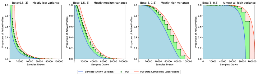
Figure 1: Proportion of pure strategy profiles that are active over the course of the $\operatorname{PSP}$ algorithm for four games with different distributions of individual utility variances.

$\operatorname{PSP}$ queries strategy profiles until they all attain a target error guarantee. Along the way, empirical estimates of variance are used to prune profiles roughly in order of increasing maximum variance $\left\lVert{}\bm{v}(\bm{s})\right\rVert{}_{\infty}$. How many profiles are active at any point thus depends on the distribution of the utility variances, because different variances lead to variations in the bounds on which $\operatorname{PSP}$ depends.

This next set of experiments is designed to highlight how the amount of work done (i.e., the number of queries placed) by $\operatorname{PSP}$ varies with the distribution of utility variances. As expected, we find that the less (resp. more) the utility variances are concentrated near the maximum variance, the smaller (resp. larger) the number of queries $\operatorname{PSP}$ requires to reach its target error guarantee.

In these experiments, we sample four games from $\mathrm{RZ}(80,2)$, where for each game, we use scaled and shifted Bernoulli additive noise variables with $d=20$ and $\gamma_{p,\bm{s}}\sim\textup{Beta}(\alpha,\beta)$ for a certain $\alpha,\beta>0$. We then run $\operatorname{PSP}$ on each game with utility range $c\doteq 22$, failure probability $\updelta\doteq 0.05$, error threshold $\varepsilon\doteq 0.2$, and geometric ratio $\beta\doteq 1.1$. For each iteration of the algorithm, we plot the proportion of strategy profiles that were active during that iteration, versus the number of samples that were drawn thus far. A point $(m,p)$ can thus be read as, “during this run of $\operatorname{PSP}$, a proportion $p$ of strategy profiles were active, and hence queried, at each of the first $m$ drawn samples.” Since $\operatorname{PSP}$ only prunes profiles at the end of each iteration, we connect these points with a decreasing step function.

We also report lower and upper (PAC-style) bounds on this $\operatorname{PSP}$ step function. The number of samples for which a strategy profile $\bm{s}$ is active is lower bounded by $\smash{m^{B}(\varepsilon,\frac{\updelta}{\left\lvert{}\Gamma\right\rvert{}};c,\left\lVert{}\bm{v}(\bm{s})\right\rVert{}_{\infty})}$ (Theorem 3.2) and upper bounded (with high probability) by $\smash{m^{\textup{PSP}}(\varepsilon,\frac{\updelta}{T\left\lvert{}\Gamma\right\rvert{}};c,\left\lVert{}\bm{v}(\bm{s})\right\rVert{}_{\infty};\beta)}$ (Lemma 4.1), respectively. Since both of these these bounds are strictly increasing in $\left\lVert{}\bm{v}(\bm{s})\right\rVert{}_{\infty}$, they also bound the number of samples for which all strategy profiles whose maximum variance is greater than or equal to $\left\lVert{}\bm{v}(\bm{s})\right\rVert{}_{\infty}$ are active. We report the proportion of active profiles corresponding to these lower and upper bounds, for all strategy profiles $\bm{s}\in\bm{S}$.

Figure 1 depicts clear differences in how quickly strategy profiles are pruned, depending on $\alpha$ and $\beta$, which dictate how utility variances are distributed. Since for each sample drawn, $\operatorname{PSP}$ queries every active strategy profile, the total area under the $\operatorname{PSP}$ curve is directly proportional to the total number of queries that were required to reach the target error guarantee. By similar reasoning, the area under the lower and upper bound curves, respectively, are also proportional to lower and (high probability) upper bounds on this total number of queries. We can therefore infer that in games where the utility variances are concentrated at a much smaller value than $\bm{v}_{\textup{max}}$ (modeled by $\textup{Beta}(0.5,3)$), query complexity is dramatically reduced through pruning. On the other hand, in games where the utility variances are concentrated closer to $\bm{v}_{\textup{max}}$ (modeled by $\textup{Beta}(5,0.5)$), pruning has a much smaller effect on query complexity.

5.3 Performance of $\operatorname{PSP}$ vs. $\operatorname{GS}$

Next, we compare the performance of the $\operatorname{PSP}$ and $\operatorname{GS}$ algorithms. Such a comparison is a difficult due to the differing use cases for the two algorithms. We run $\operatorname{PSP}$ when we have a target error $\varepsilon$ in mind, and the algorithm optimizes the query complexity to reach that target. We run $\operatorname{GS}$ when we are given a data set consisting of $m$ samples together with responses to the queries corresponding to each sample, and the algorithm outputs the tightest possible guarantee on the confidence radius. Since $\operatorname{PSP}$ has been our focus in this paperProportion, in our plots, we use the horizontal axis for the independent variable $\varepsilon$, and the vertical axis for the resulting query and data complexities. When plotting results from the $\operatorname{GS}$ algorithm, however, we plot as if the vertical axis were the independent variable and the horizontal axis, dependent. It is important that our results are interpreted this way, as $\operatorname{GS}$ is not able to provide any strong a priori guarantees regarding the query complexity required to produce a certain $\varepsilon$ guarantee without access to the true maximum utility variance of a game.

We experiment with congestion games sampled from $\mathrm{RC}(3,3,2)$, and Bernoulli additive noise variables with $d=20$ in two settings: a Single Game and Many Games. In the Single Game setting, we sample one congestion game and draw each $\gamma_{p,\bm{s}}\sim\textup{Beta}(1.5,3)$. We then run $\operatorname{GS}$ using uniform empirical Bennett bounds 10 times at a variety of sample sizes $m$, and $\operatorname{PSP}$ 10 times for a variety of target error $\varepsilon$. Using $\textup{Beta}(1.5,3)$ models a plausible empirical game where most utilities have moderate variance, but some outlier utilities have high variance. In the Many Games setting, we instead sample 9 congestion games and draw each $\gamma_{p,\bm{s}}\sim\textup{Beta}(1.5+i,3+j)$, using each $(i,j)\in\{-0.1,0,0.1\}^{2}$ in one game. For each of these 9 games, we then run $\operatorname{GS}$ once for a variety of sample sizes $m$, and $\operatorname{PSP}$ once for a variety of target errors $\varepsilon$.

On each graph in Figure 2, we plot the following:

• GS-H: $\operatorname{GS}$ using Hoeffding Bounds (Theorem 3.1).

• GS-B: $\operatorname{GS}$ using uniform Bennett bounds (Theorem 3.2) and known maximum variance.

• GS-EB: $\operatorname{GS}$ using uniform empirical Bennett bounds, with dependence on $\left\lVert{}\hat{\bm{v}}\right\rVert{}_{\infty}$ rather than individual empirical variances Areyan Viqueira et al. (2020).

• GS-EB Upper Bound: PAC-style upper bound on the empirical Bennett data complexity (Theorem 3.3).

• PSP: $\operatorname{PSP}$ using Hoeffding and Empirical Bennett bounds (Algorithm 1).

• PSP Upper Bound: PAC-style upper bound on the query complexity of $\operatorname{PSP}$ (Theorem 4.2).

For the algorithms that compute an empirical Bennett bound (i.e., GS-EB and PSP), we plot each run of the algorithm in the single game case, and a min-max interval in the many games case.

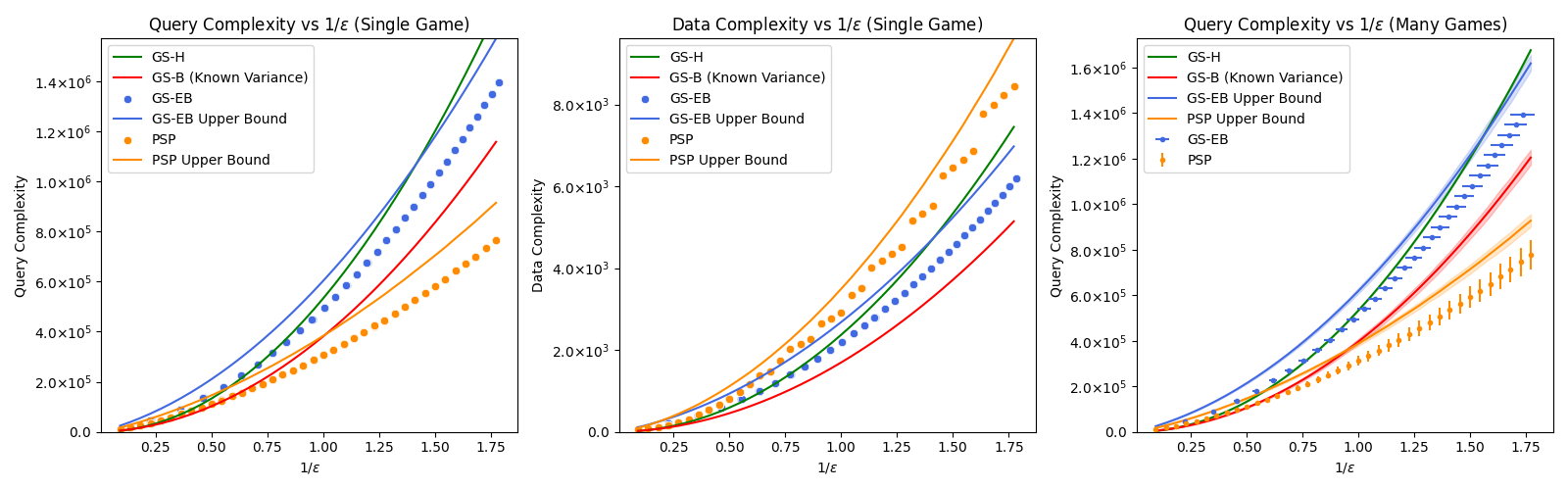
Figure 2: Performance comparisons of $\operatorname{GS}$ using Hoeffding and Uniform Empirical Bennett vs. $\operatorname{PSP}$, along with their corresponding bounds, for various sample sizes $m$ and target errors $\varepsilon$, respectively.

In the Single Game graphs, although we plot 10 runs of both algorithms, all that is visible is a single run’s worth of points. This suggests that for a single game, from one run to another, there is little variation in the $\varepsilon$ guarantees produced by $\operatorname{GS}$ or in the query complexities of $\operatorname{PSP}$. On the other hand, in the Many Games graph, we see much more variation, again showing that changes in the distribution of utility variances impact these algorithms.

We observe that $\operatorname{PSP}$ significantly outperforms $\operatorname{GS}$-EB in query complexity, even consuming fewer queries than $\operatorname{GS}$-B, which assumes known maximum variance, while performing significantly worse with respect to data complexity, even when compared to $\operatorname{GS}$-H. The same relations hold when comparing $\operatorname{PSP}$ Upper Bound to $\operatorname{GS}$-EB Upper Bound. We thus conclude that $\operatorname{PSP}$ outperforms $\operatorname{GS}$ using uniform empirical Bennett bounds, thus empirically outperforming the state-of-the-art.

In summary, $\operatorname{PSP}$ is the preferred algorithm when minimizing query complexity is paramount; it was designed to be thus, and our experiments confirm that it achieves this desideratum. An exception is the pathological case where all utility variances are uniform, in which case $\operatorname{PSP}$ results in both greater query complexity and greater data complexity. We note anecdotally, however, that even in games with variances concentrated near the maximum variance ($\gamma_{p,\bm{s}}\sim\textup{Beta}(3,1.5)$), $\operatorname{PSP}$ still matches $\operatorname{GS}$ in terms of query complexity; it is only ever marginally better or worse.

6 Experiments with Properties

Upon termination, $\operatorname{PSP}$ returns an empirical estimate of a simulation-based game with utilities which, with probability at least $1-\updelta$, are no more than some target error $\varepsilon$ away from the true utilities. It follows that all well-behaved (i.e., Lipschitz continuous in utilities) properties of this game can likewise be learned. In this section, we further investigate through experimentation the learnability of two key properties of games, namely regret (i.e., equilibria) and power-mean welfare. Our findings can be summarized as follows:

• Although regret is 2-Lipschitz, and thus amenable to statistical EGTA in theory, we exhibit games in which learning better approximations of the game steadily grants access to better $\varepsilon$-equilibria, as well as games where this is often not the case.

• We demonstrate that $\rho$-power-mean welfare is not well behaved for certain values of $\rho$, as the average supremum error between the empirical estimates and the true of $\rho$-power-mean welfare can grow very large.

6.1 Regret

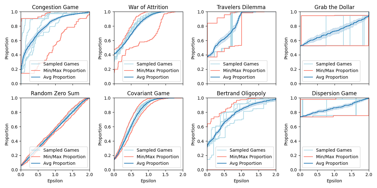
Figure 3: Average proportion of pure strategy profiles that are $\varepsilon$-Nash equilibria over 100 sampled games vs. $\varepsilon$ for 8 different GAMUT games. Exact proportions for 5 of the 100 sampled games are also plotted, along with the maximum and minimum proportions over the 100 games.

We ran these experiments on randomly generated game instances from eight GAMUT game classes. For each game class, we generate 100 games with all parameters randomized except those needed to fix the game size between 300 and 350 pure strategy profiles (e.g., for Random Zero Sum games, we fix the number of strategies per player at 18, which yields $18^{2}=324$ pure strategy profiles).

In Figure 3, we plot the proportion of pure strategy profiles that are $\varepsilon$-Nash equilibria for various values of $\varepsilon>0$. A spurious equilibrium is an $\varepsilon$-equilibrium that is not also a Nash equilibrium. The figure shows how the rate at which better approximations of the game (smaller $\varepsilon$) eliminate spurious equilibria can depend on the game’s inherent structure. In Random Zero Sum games, for example, spurious equilibria can be steadily removed as stronger $\varepsilon$ guarantees are attained.

On the other hand, in Grab the Dollar and Dispersion, we see phase transitions. In all instances of these games, there is a cutoff $\varepsilon^{*}$ s.t. for all $\varepsilon<\varepsilon^{*}$, each $\varepsilon$-Nash equilibrium is also a Nash equilibrium (i.e., there are no spurious $\varepsilon$-Nash equilibria), and for all $\varepsilon\geq\varepsilon^{*}$, each $\varepsilon$-Nash equilibrium is also an $\varepsilon^{*}$-Nash equilibrium (i.e., all spurious Nash equilibria are $\varepsilon^{*}$-Nash equilibria). When $\varepsilon^{*}$ is large, the first case renders it trivial (i.e., very few samples are required) to produce an $\varepsilon$-uniform approximation, for $\varepsilon<\varepsilon^{*}$ and near $\varepsilon^{*}$, and hence learn all Nash equilibria. On the other hand, when $\varepsilon^{*}$ is very small, the second case renders even spurious equilibria good approximate Nash equilibria, which again can be learned from just a few samples. As a result, statistical EGTA methodology may be overkill in these games in some cases. Still, when $\varepsilon^{*}$ is not small enough to capture good approximate equilibria, and simultaneously not large enough to render learning trivial, our EGTA methods provide a means of efficiently learning Nash equilibria, as they are designed to gracefully adapt to the inherent, yet a priori unknown, difficulty of the task at hand.

6.2 Non-Lipschitz Properties

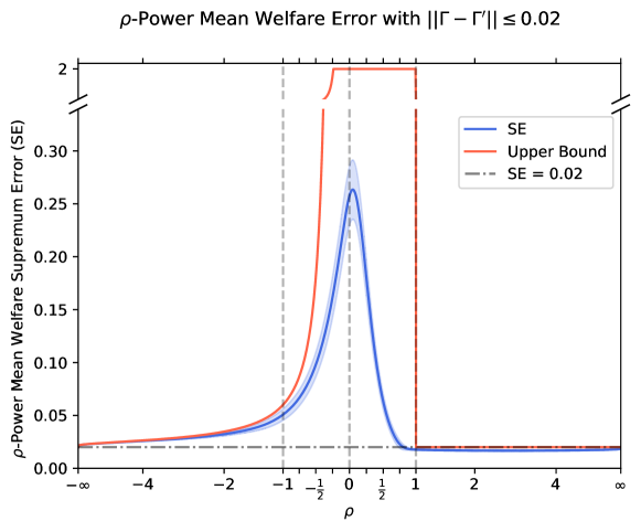
Figure 4: Average supremum error between the empirical estimates and the true $\rho$-power-mean welfares at each strategy profile for various values of $\rho$. Vertical lines are plotted at each $\rho\in\{-1,0,1\}$.

In this experiment, we sample a congestion game $\Gamma$ from $\mathrm{RC}(3,3,2)$, and then uniformly draw 100 arbitrary normal form games $\Gamma^{\prime}$, each satisfying $\left\lVert{}\Gamma-\Gamma^{\prime}\right\rVert{}_{\infty}\leq\varepsilon\doteq 0.02$. Each draw represents a possible empirical estimate of $\Gamma$ that might be learned by $\operatorname{PSP}$ or $\operatorname{GS}$. For values of $\rho\in[-10,10]$, we then plot the average of the supremum, across all strategy profiles $\bm{s}\in\bm{S}$, of the errors between the empirical estimate of the $\rho$-power-mean welfare at $\bm{s}$ and the (actual) $\rho$-power-mean welfare at $\bm{s}$. In Figure 4, we observe that $\rho$-power-mean welfare is $\varepsilon$-well-estimated for $\rho>1$, as expected, and is also fairly well-estimated for $\rho<-1$. Since $\rho$-power-mean welfare is $\max_{p\in P}\bm{w}_{p}^{\nicefrac{{1}}{{\rho}}}$-Lipschitz continuous, we expect high error as $\rho\to 0^{-}$, and as it is Lipschitz discontinuous for $\rho\in[0,1)$, we also expect high error in this region.

Although power means are not Lipschitz-continuous, for $\rho\in[0,1)$, and may consequently be more difficult to estimate than Lipschitz-continuous properties, their sample complexity is not necessarily unbounded. In particular, for $\rho=0$, the difficulty with estimating the power mean stems from the fact that the derivative can grow in an unbounded fashion as some utility value approaches zero. Said derivatives, however, are only unbounded when that utility value is exactly zero. Thus, as we move away from this singularity, our estimates will converge, but the rate of convergence may be slow. In contrast, other interesting properties of games, like the price of anarchy, are not even continuous—the price of anarchy depends on the maximum welfare at an equilibrium, which is not a continuous function of utilities—and thus no convergent estimator can exist for them.

7 Conclusion

The main contributions of this paper are twofold. First, we present a simple yet general framework in which to analyze game properties, which recovers known results on the learnability of game-theoretic equilibria. We show that other properties of interest also fit into our framework, e.g., power-mean and Gini social welfare. These choices show the flexibility and ease with which our methodology may be applied. Furthermore, by analyzing these simple choices, we observe that not all game properties are well behaved.

Second, we develop a novel algorithm that learns well-behaved game properties with provable efficiency guarantees. The key new insights that our paper offers are efficiency bounds with a dependence on utility variance, not just its range, as shown previously by Tuyls et al. (2020). While Areyan Viqueira et al. (2020) also employed variance-aware bounds in their regret-based pruning algorithm, they did not provide any efficiency guarantees. We improve upon their variance-aware bounds by deriving a novel sub-gamma tail bound, and we achieve efficiency guarantees via a novel progressive sampling schedule. In future work, these improvements could be combined with Areyan Viqueira et al.’s regret-based pruning to yield still tighter efficiency guarantees when the property of interest is specifically regret: i.e., equilibria.

While our algorithms are nearly optimal for uniformly approximating simulation-based games, which is sufficient for learning well-behaved game properties, Areyan Viqueira et al.’s regret-based pruning algorithm, which learns non-uniform approximations, demonstrates that doing so is not always necessary. In future work, we plan to develop additional pruning criteria that increase efficiency by pruning any utilities that are not relevant to learning the property at hand. We are hopeful that a generic algorithm can be developed that prunes efficiently while maintaining the generality of our theory, rather than resorting to multiple algorithms, each of which learns a specific property.

Appendix A Proofs of Lipschitz Properties in Games

A.1 Lipschitz Calculus

Theorem A.1 (Lipschitz Facts).

1. Linear Combination: If $g_{1:m}$ are $\lambda_{1:m}$-Lipschitz, all w.r.t. the same two norms, and $\bm{w}\in\mathbb{R}^{m}$, then the function $x\mapsto\bm{w}\cdot g(x)$ is $\sum_{i=1}^{m}\lambda_{i}\left\lvert{}\bm{w}_{i}\right\rvert{}$-Lipschitz. 2. Composition: If $h:A\to B$ and $g:B\to C$ are $\lambda_{h}$- and $\lambda_{g}$-Lispchitz w.r.t. norms $\left\lVert{}\cdot\right\rVert{}_{A}$, $\left\lVert{}\cdot\right\rVert{}_{B}$, & $\left\lVert{}\cdot\right\rVert{}_{C}$, then $(g\circ h):A\to C$ is $\lambda_{h}\lambda_{g}$ Lispchitz w.r.t. $\left\lVert{}\cdot\right\rVert{}_{A}$ and $\left\lVert{}\cdot\right\rVert{}_{C}$. 3. The infimum and supremum operations are 1-Lipschitz continuous: i.e., if for all $x\in\mathcal{X}$, $f(x;\bm{u})$ is $\lambda$-Lipschitz in $\bm{u}$ then $\inf_{x\in\mathcal{X}}f(x;\bm{u})$ is also $\lambda$-Lipschitz in $\bm{u}$. Likewise, for the supremum.

A.2 Mixed Utilities are Lipschitz Continuous

Lemma A.1.

The functional $f:\bm{{S}^{\diamond}}\times(\bm{S}\to\mathbb{R}^{|P|})\to\mathbb{R}$ that computes a player’s utility given a mixed strategy, e.g., $\bm{u}^{\diamond}_{p}(\bm{s})$ for some $p\in P$, is 1-Lipschitz continuous in utilities.

Proof.

The functional $f$ converts a player’s utility at a mixed strategy profile into the expected value of their utility over pure strategy profiles, given the mixture. This operation is $1$-Lipschitz, because taking an expectation is a convex combination, which is 1-Lipschitz by the linear combination rule, because utilities are 1-Lipschitz themselves. ∎

A.3 Lipschitz Continuous Game Properties

Theorem A.2 (Lipschitz Properties).

1. The Gini social welfare function is 1-Lipschitz: i.e.,

$$\sup_{\bm{s}\in\bm{S}}\left\lvert{}\operatorname{W}_{\bm{w}^{\downarrow}}(s;\bm{u})-\operatorname{W}_{\bm{w}^{\downarrow}}(s;\bm{u}^{\prime})\right\rvert{}\leq\left\lVert{}\bm{u}-\bm{u}^{\prime}\right\rVert{}_{\infty}\enspace.$$

2. Given a player $p\in P$, their adversarial value is 1-Lipschitz: i.e.,

$$\sup_{s\in S_{p}}\left\lvert{}\mathrm{A}_{p}(s;\bm{u})-\mathrm{A}_{p}(s;\bm{u}^{\prime})\right\rvert{}\leq\left\lVert{}\bm{u}-\bm{u}^{\prime}\right\rVert{}_{\infty}\enspace.$$

3. Pure regret is 2-Lipschitz: i.e.,

$$\sup_{\bm{s}\in\bm{S}}\left\lvert{}\operatorname{Reg}(\bm{s};\bm{u})-\operatorname{Reg}(\bm{s};\bm{u}^{\prime})\right\rvert{}\leq 2\left\lVert{}\bm{u}-\bm{u}^{\prime}\right\rVert{}_{\infty}\enspace.$$

Proof.

1. Fix an arbitrary strategy profile $\bm{s}\in\bm{S}$. Recall the definition of Gini social welfare, namely $\operatorname{W}_{\bm{w}^{\downarrow}}(\bm{s};\bm{u})\doteq\bm{w}^{\downarrow}\cdot\bm{u}^{\uparrow}(\bm{s})$. Because $\bm{w}^{\downarrow}\in\triangle^{|P|}$ is decreasing and $\bm{u}^{\uparrow}(\bm{s})$ is increasing, it holds that $\operatorname{W}_{\bm{w}^{\downarrow}}(\bm{s};\bm{u})=\inf_{\bm{w}\in\Pi(\bm{w}^{\downarrow})}\bm{w}\cdot\bm{u}^{\uparrow}(\bm{s})=\inf_{\bm{w}\in\Pi(\bm{w}^{\downarrow})}\bm{w}\cdot\bm{u}(\bm{s})$, where $\Pi(\bm{w}^{\downarrow})$ is the set of all possible permutations of $\bm{w}^{\downarrow}$. Now, since $\left\lVert{}\bm{w}^{\downarrow}\right\rVert{}_{1}=1$, the dot product is a convex combination, which is $1$-Lipschitz. Taking an infimum of $1$-Lipschitz functions is also $1$-Lipschitz. Thus, by composition, $\operatorname{W}_{\bm{w}^{\downarrow}}(\bm{s};\bm{u})$ is $1\cdot 1=1$-Lipschitz. As $\bm{s}$ was arbitrary, the result holds for all $\bm{s}\in\bm{S}$.

2. Fix an arbitrary strategy $s\in S_{p}$. By definition, $\mathrm{A}_{p}(s;\bm{u})=\inf_{\bm{s}\in\bm{S}\mid\bm{s}_{p}=s}\bm{u}_{p}(\bm{s})$. Utilities are 1-Lipschitz continuous in themselves. Taking an infimum of $1$-Lipschitz functions is also $1$-Lipschitz. Thus, by composition, $\mathrm{A}_{p}(s;\bm{u})$ is $1\cdot 1=1$-Lipschitz. As $s$ was arbitrary, the result holds for all $s\in S_{p}$.

3. Fix an arbitrary strategy profile $\bm{s}\in\bm{S}$. By definition,

$$\operatorname{Reg}(\bm{s};\bm{u})=\max_{p\in P}\operatorname{Reg}_{p}(\bm{s};\bm{u})=\max_{p\in P}\sup_{\bm{s}^{\prime}\in\operatorname{Adj}_{p,\bm{s}}}\left(\bm{u}_{p}(\bm{s}^{\prime})-\bm{u}_{p}(\bm{s})\right)\enspace.$$

Utilities are 1-Lipschitz continuous in themselves. The difference between utilities is then 2-Lipschitz, because it can be construed as the sum of two 1-Lipschitz continuous functions, and negating a function does not change its Lipschitz constant. Finally, as the maximum and supremum operations are both 1-Lipschitz, by composition, $\operatorname{Reg}(\bm{s};\bm{u})$ is $1\cdot 1\cdot(1+1)=2$-Lipschitz. As $\bm{s}$ was arbitrary, the result holds for all $\bm{s}\in\bm{S}$. ∎

Figure A.5: Abstract syntax tree derivation of the Lipschitz constant for $\mathrm{A}_{p}(s;\bm{u})$, left, $\operatorname{W}_{\bm{w}^{\downarrow}}(\bm{s};\bm{u})$, middle, and $\operatorname{Reg}(\bm{s};\bm{u})$, right. The empty parentheses $(\cdot)$ indicate the arguments to the operators, while the filled parentheses (e.g., $(1)$) are filled with the respective arguments’ Lipschitz constants.

A.4 Uniform Approximations of Game Properties

We now show Theorem 2.1.

See 2.1

Proof.

To show (1), first note the following:

$$\sup_{x\in\mathcal{X}}f(x;\bm{u})-\sup_{x\in\mathcal{X}}f(x;\bm{u}^{\prime})\leq\sup_{x\in\mathcal{X}}(f(x;\bm{u})-f(x;\bm{u}^{\prime}))\leq\sup_{x\in\mathcal{X}}\left\lvert{}f(x;\bm{u})-f(x;\bm{u}^{\prime})\right\rvert{}\leq\lambda\varepsilon\enspace.$$

The final inequality follows from Observation 2.1. Symmetric reasoning yields $\sup_{x\in\mathcal{X}}f(x;\bm{u}^{\prime})-\sup_{x\in\mathcal{X}}f(x;\bm{u})\leq\lambda\varepsilon$, implying the statement for suprema. We obtain a similar result for infima, by noting that suprema of $-f$ are infima of $f$.

The infimum claim of (2) follows similarly from the supremum claim, and the supremum claim holds as follows, where the first inequality is due to Observation 2.1, the second, to the assumption that $\hat{x}$ is $\alpha$-optimal, and the third, to (1):

$$f(\hat{x};\bm{u})\geq f(\hat{x};\bm{u}^{\prime})-\lambda\varepsilon\geq\sup_{x\in\mathcal{X}}f(x;\bm{u}^{\prime})-\lambda\varepsilon-\alpha\geq\sup_{x\in\mathcal{X}}f(x;\bm{u})-2\lambda\varepsilon-\alpha\enspace.$$

∎

We now show Theorem 2.2.

See 2.2

Proof.

By Observation 2.1,

$$\forall x\in F_{0}(\bm{u}):\,f(x;\bm{u})=v^{*}\implies f(x;\bm{u}^{\prime})-v^{*}\leq\lambda\varepsilon\implies x\in F_{\lambda\varepsilon}(\bm{u}^{\prime})$$

$$\forall x\in F_{\lambda\varepsilon}(\bm{u}^{\prime}):\,f(x;\bm{u}^{\prime})-v^{*}\leq\lambda\varepsilon\implies f(x;\bm{u})-v^{*}\leq\lambda\varepsilon+\lambda\varepsilon=2\lambda\varepsilon\implies x\in F_{2\lambda\varepsilon}(\bm{u})$$

∎

Appendix B Proofs of Finite-Sample Bounds for Expected NFGs

We begin by showing  Theorem 3.2.

See 3.2

Proof.

Bennett’s Inequality (1962) states that

$${{\operatorname*{\mathbb{P}}\!\left(\bar{X}\geq\operatorname*{\mathbb{E}}[\bar{X}]+\varepsilon\right)\leq\exp\left(-\frac{m\sigma_{\Gamma}^{\smash{2}}}{c_{\Gamma}}h\left(\frac{c_{\Gamma}\varepsilon}{\sigma_{\Gamma}^{\smash{2}}}\right)\right)}}$$ (1)

where $h(x)\doteq(1+x)\ln(1+x)-x$ for all $x\geq 0$. Substituting $-\bar{X}$ for $\bar{X}$, we get an identical reverse-tail bound, which when combined with a union bound yields

$${{\operatorname*{\mathbb{P}}\!\left(\left\lvert{}\bar{X}-\operatorname*{\mathbb{E}}[\bar{X}]\right\rvert{}\geq\varepsilon\right)\leq 2\exp\left(-\frac{m\sigma_{\Gamma}^{\smash{2}}}{c_{\Gamma}}h\left(\frac{c_{\Gamma}\varepsilon}{\sigma_{\Gamma}^{\smash{2}}}\right)\right)}}$$

Taking the variance proxy $\sigma_{\Gamma}^{2}$ to be $\bm{v}_{p}(\bm{s})$ and the scale proxy $c_{\Gamma}$ to be $c$, we obtain the following guarantee on the deviation between $\bm{u}_{p}(\bm{s};\mathscr{D})$ and $\hat{\bm{u}}_{p}(\bm{s};\bm{Y})$ for a single $\smash{(p,\bm{s})\in\bm{\mathcal{I}}}$ :

$${{\operatorname*{\mathbb{P}}\!\left(\left\lvert{}\hat{\bm{u}}_{p}(\bm{s};\bm{Y})-\bm{u}_{p}(\bm{s};\mathscr{D})\right\rvert{}\geq\varepsilon\right)\leq 2\exp\left(-\frac{m\bm{v}_{p}(\bm{s})}{c}h\left(\frac{c\varepsilon}{\bm{v}_{p}(\bm{s})}\right)\right)}}$$

Thus, to arrive at an $\varepsilon$-radius confidence interval in which $\left\lvert\bm{u}_{p}(\bm{s};\mathscr{D})-\hat{\bm{u}}_{p}(\bm{s};\bm{Y})\right\rvert\leq\varepsilon$ with probability at least $1-\updelta$, we upper bound the right hand side by $\updelta$. This constraint is achieved with

$$m^{B}(\varepsilon,\updelta;c,\bm{v}_{p}(\bm{s}))\doteq\frac{c^{2}\ln\left(\frac{2}{\updelta}\right)}{\bm{v}_{p}(\bm{s})h\left(\frac{c\varepsilon}{\bm{v}_{p}(\bm{s})}\right)}\leq 2\ln\frac{2}{\updelta}\left(\frac{c}{3\varepsilon}+\frac{\bm{v}_{p}(\bm{s})}{\varepsilon^{2}}\right)$$ (2)

samples. Notice that $m^{B}$ is monotonically increasing and concave in $\bm{v}_{p}(\bm{s})$ (this can be confirmed by analyzing its first and second derivatives).

To obtain a similar $\varepsilon$-$\updelta$ guarantee over strategy profile $\bm{s}$, namely $\left\lVert{}\bm{u}(\bm{s};\mathscr{D})-\hat{\bm{u}}(\bm{s};\bm{Y})\right\rVert{}_{\infty}\leq\varepsilon$, it suffices (applying a union bound over $|P|$ players) to draw at least

$$\max_{p\in P}m^{B}(\varepsilon,\nicefrac{{\updelta}}{{|P|}};c,\bm{v}_{p}(\bm{s}))=m^{B}(\varepsilon,\nicefrac{{\updelta}}{{|P|}};c;\left\lVert{}\bm{v}(\bm{s})\right\rVert{}_{\infty})\leq 2\ln\frac{2|P|}{\updelta}\left(\frac{c}{3\varepsilon}+\frac{\left\lVert{}\bm{v}(\bm{s})\right\rVert{}_{\infty}}{\varepsilon^{2}}\right)$$ (3)

samples. Here, we must simulate a strategy profile until the utility indices of all players are well-estimated. Thus, the bottleneck is the worst-case (per-player) variance, which explains the use of the infinity norm over players.

Now note that the total data complexity of $\varepsilon$-$\updelta$ estimating a game is the maximum data complexity of $\varepsilon$-$\updelta$ estimating any strategy profile. The total data complexity is then

$$m \leq\max_{\bm{s}\in\bm{S}}2\ln\frac{2\left\lvert{}\Gamma\right\rvert{}}{\updelta}\left(\frac{c}{3\varepsilon}+\frac{\left\lVert{}\bm{v}(\bm{s})\right\rVert{}_{\infty}}{\varepsilon^{2}}\right)$$ (4)

$$=2\ln\frac{2\left\lvert{}\Gamma\right\rvert{}}{\updelta}\left(\frac{c}{3\varepsilon}+\max_{\bm{s}\in\bm{S}}\frac{\left\lVert{}\bm{v}(\bm{s})\right\rVert{}_{\infty}}{\varepsilon^{2}}\right)$$ (5)

$$=2\ln\frac{2\left\lvert{}\Gamma\right\rvert{}}{\updelta}\left(\frac{c}{3\varepsilon}+\frac{\left\lVert{}\bm{v}\right\rVert{}_{\infty}}{\varepsilon^{2}}\right)$$ (6)

$$\max_{\bm{s}\in\bm{S}}m^{B}(\varepsilon,\nicefrac{{\updelta}}{{\left\lvert{}\Gamma\right\rvert{}}};c,\left\lVert{}\bm{v}(\bm{s})\right\rVert{}_{\infty}))=m^{B}(\varepsilon,\nicefrac{{\updelta}}{{\left\lvert{}\Gamma\right\rvert{}}};c;\left\lVert{}\bm{v}\right\rVert{}_{\infty})\leq 2\ln\frac{2\left\lvert{}\Gamma\right\rvert{}}{\updelta}\left(\frac{c}{3\varepsilon}+\frac{\left\lVert{}\bm{v}\right\rVert{}_{\infty}}{\varepsilon^{2}}\right)\enspace.$$ (7)

Similarly, to arrive at the query complexity, we simply sum rather than maximize over strategy profiles:

$$m \leq\sum_{\bm{s}\in\bm{S}}\max_{p\in P}2\ln\frac{2\left\lvert{}\Gamma\right\rvert{}}{\updelta}\left(\frac{c}{3\varepsilon}+\frac{\bm{v}_{p}(\bm{s})}{\varepsilon^{2}}\right)$$ (8)

$$=2\ln\frac{2\left\lvert{}\Gamma\right\rvert{}}{\updelta}\left(\frac{c\left\lvert{}\Gamma\right\rvert{}}{3\varepsilon}+\sum_{\bm{s}\in\bm{S}}\max_{p\in P}\frac{\bm{v}_{p}(\bm{s})}{\varepsilon^{2}}\right)$$ (9)

$$=2\ln\frac{2\left\lvert{}\Gamma\right\rvert{}}{\updelta}\left(\frac{c\left\lvert{}\Gamma\right\rvert{}}{3\varepsilon}+\frac{\left\lVert{}\bm{v}\right\rVert{}_{1,\infty}}{\varepsilon^{2}}\right)\enspace.$$ (10)

$$\sum_{\bm{s}\in\bm{S}}\left\lceil m^{B}(\varepsilon,\nicefrac{{\updelta}}{{\left\lvert{}\Gamma\right\rvert{}}};c,\left\lVert{}\bm{v}(\bm{s})\right\rVert{}_{\infty})\right\rceil$$

$$\leq \left\lvert{}\bm{S}\right\rvert{}+\sum_{\bm{s}\in\bm{S}}m^{B}(\varepsilon,\nicefrac{{\updelta}}{{\left\lvert{}\Gamma\right\rvert{}}};c,\left\lVert{}\bm{v}(\bm{s})\right\rVert{}_{\infty})$$

$$\leq \left\lvert{}\bm{S}\right\rvert{}+\left\lvert{}\bm{S}\right\rvert{}m^{B}\left(\varepsilon,\nicefrac{{\updelta}}{{\left\lvert{}\Gamma\right\rvert{}}};c,\frac{1}{\left\lvert{}\bm{S}\right\rvert{}}\sum_{\bm{s}\in\bm{S}}\left\lVert{}\bm{v}(\bm{s})\right\rVert{}_{\infty}\right) [{\textup{Jensen's Inequality + Concavity of $m^{B}$}}]$$

$$= \left\lvert{}\bm{S}\right\rvert{}+m^{B}(\varepsilon,\nicefrac{{\updelta}}{{\left\lvert{}\Gamma\right\rvert{}}};c\left\lvert{}\bm{S}\right\rvert{},\left\lVert{}\bm{v}\right\rVert{}_{1,\infty}) [{\textup{Definition of $m^{B}$ + Algebra}}]$$

$$\leq \left\lvert{}\bm{S}\right\rvert{}+2\ln\frac{2\left\lvert{}\Gamma\right\rvert{}}{\updelta}\left(\frac{c\left\lvert{}\bm{S}\right\rvert{}}{3\varepsilon}+\frac{\left\lVert{}\bm{v}\right\rVert{}_{1,\infty}}{\varepsilon^{2}}\right)\enspace.$$

∎

In order to show Theorem 3.3, we prove a more general theorem.  Theorem 3.3 then follows through the application of a union bound over all utilities. We begin with the following Lemma:

Lemma B.1.

Let $X\doteq(X_{1},\dots,X_{m})$ be a vector of independent random variables each with finite variance, assume that $|X_{i}-\mathbb{E}[X_{i}]|\leq c$ almost surely for all $i$, and define $\bar{X}\stackrel{{\scriptstyle.}}{{=}}\frac{1}{m}\sum_{i=1}^{m}X_{i}$. Then $\hat{v}(X)\stackrel{{\scriptstyle.}}{{=}}\frac{1}{m-1}\sum_{i=1}^{m}(X_{i}-\bar{X})^{2}$ is $\left(1,\frac{c^{2}m}{4(m-1)^{2}}\right)$-self-bounding, and hence by Boucheron et al. (2000), with probability at least $1-\updelta$ over the draw of $X$, it holds that

$$\operatorname*{\mathbb{E}}[\hat{v}(X)]\leq\hat{v}(X)+\frac{2c^{2}\ln\frac{1}{\updelta}}{3m}+\sqrt{\left(\frac{1}{3}+\frac{1}{2\ln\frac{1}{\updelta}}\right)\left(\frac{c^{2}\ln\frac{1}{\updelta}}{m-1}\right)^{2}+\frac{2c^{2}\hat{v}(X)\ln\frac{1}{\updelta}}{m}}\enspace.$$

Furthermore, we also have that $\hat{v}(X)$ is $\left(\frac{m}{m-1},0\right)$-self-bounding, and hence by Boucheron et al. (2009), with probability at least $1-\updelta$ over the draw of $X$, it holds that

$$\hat{v}(X)\leq\operatorname*{\mathbb{E}}[\hat{v}(X)]+\frac{2m+1}{6(m-1)}\cdot\frac{c^{2}\ln\frac{3}{\updelta}}{m}+\sqrt{\frac{2c^{2}v\ln\frac{3}{\updelta}}{m-1}}\enspace.$$

Proof.

Let $\textsf{Z}(X)\stackrel{{\scriptstyle.}}{{=}}\hat{v}(X)$, and for each index $j$, define $\textsf{Z}_{j}(X)$ by

$$\textsf{Z}_{j}(X)\stackrel{{\scriptstyle.}}{{=}}\frac{1}{m-1}\sum_{i=1,i\neq j}^{m}(X_{i}-\bar{X}_{\setminus j})^{2}$$

where $\bar{X}_{\setminus j}$ denotes $\sum_{i=1,i\neq j}X_{i}$. We will first show that $\textsf{Z}_{j}(X)=\textsf{Z}(X)-\frac{1}{m}(X_{j}-\bar{X}_{\setminus j})^{2}$, as this form comes in handy many times. Starting from the definition of $\textsf{Z}_{j}(X)$, we add and subtract $\frac{1}{m-1}(X_{j}-X_{\setminus j})^{2}$ to the entire expression, and then add and subtract $\bar{X}$ to the argument of the sum, to obtain:

$$\textsf{Z}_{j}(X) =\frac{1}{m-1}\left(\sum_{i=1}^{m}(X_{i}-\bar{X}_{\setminus j})^{2}-(X_{j}-\bar{X}_{\setminus j})^{2}\right)$$

$$=\frac{1}{m-1}\Bigg{(}\sum_{i=1}^{m}((X_{i}-\bar{X})+(\bar{X}-\bar{X}_{\setminus j}))^{2}-(X_{j}-\bar{X}_{\setminus j})^{2}\Bigg{)}$$

$$=\frac{1}{m-1}\Bigg{(}\sum_{i=1}^{m}(X_{i}-\bar{X})^{2}+2\sum_{i=1}^{m}(X_{i}-\bar{X})(\bar{X}-\bar{X}_{\setminus j})+\sum_{i=1}^{m}(\bar{X}-\bar{X}_{\setminus j})^{2}-(X_{j}-\bar{X}_{\setminus j})^{2}\Bigg{)}.$$

Since $\bar{X}-\bar{X}_{\setminus j}$ is independent of $i$ and $\sum_{i=1}^{m}(X_{i}-\bar{X})=0$, we have that $2\sum_{i=1}^{m}(X_{i}-\bar{X})(\bar{X}-\bar{X}_{\setminus j})=0$. This, in combination with the definition of $\textsf{Z}(X)$, gives us

$$\textsf{Z}_{j}(X) =\textsf{Z}(X)+\frac{1}{m-1}\left[m(\bar{X}-\bar{X}_{\setminus j})^{2}-(X_{j}-\bar{X}_{\setminus j})^{2}\right].$$

But we have that $\bar{X}=\frac{1}{m}X_{j}+\frac{m-1}{m}\bar{X}_{\setminus j}$, which implies that

$$\textsf{Z}_{j}(X) =\textsf{Z}(X)+\frac{1}{m-1}\left[m\left(\frac{1}{m}X_{j}-\frac{1}{m}\bar{X}_{\setminus j}\right)^{2}-(X_{j}-\bar{X}_{\setminus j})^{2}\right]$$

$$=\textsf{Z}(X)+\frac{1}{m-1}\left[-\frac{m-1}{m}\left(X_{j}-\bar{X}_{\setminus j}\right)^{2}\right]$$

$$=\textsf{Z}(X)-\frac{1}{m}\left(X_{j}-\bar{X}_{\setminus j}\right)^{2}.$$ (11)

We will now show that Z is a $\left(1,\frac{c^{2}m}{4(m-1)^{2}}\right)$-self-bounding function with scale $c^{2}/m$. Since Equation 11 implies that $\textsf{Z}(X)=\textsf{Z}_{j}(X)+\frac{1}{m}\left(X_{j}-\bar{X}_{\setminus j}\right)^{2}$ for all indices $j$, and the definition of $X$ guarantees that $X_{j}-\bar{X}_{\setminus j}\leq c$ for all indices $j$, we have that for all indices $j$, it must be the case that

$$\textsf{Z}_{j}(X)\leq\textsf{Z(X)}\leq\textsf{Z}_{j}(X)+\frac{c^{2}}{m}.$$

Finally, we will now show that

$$\sum_{i=1}^{m}(\textsf{Z}(X)-\textsf{Z}_{j}(X))\leq Z(X)+\frac{c^{2}m}{4(m-1)^{2}}.$$

By applying Equation 11, we have

$$\sum_{j=1}^{m}(\textsf{Z}(X)-\textsf{Z}_{j}(X)) =\sum_{j=1}^{m}\left(\textsf{Z}(X)-\textsf{Z(X)}+\frac{1}{m}(X_{j}-\bar{X}_{\setminus j})^{2}\right)$$

$$=\frac{1}{m}\sum_{j=1}^{m}(X_{j}-\bar{X}_{\setminus j})^{2}$$

But by the definition of $X$, it holds that $\bar{X}_{\setminus j}=\frac{1}{m-1}\left(m\bar{X}-X_{j}\right)$. Hence, we have that

$$\sum_{j=1}^{m}(\textsf{Z}(X)-\textsf{Z}_{j}(X)) =\frac{1}{m}\sum_{j=1}^{m}\left(\frac{m}{m-1}X_{j}-\frac{m}{m-1}\bar{X}\right)^{2}$$

$$=\frac{m}{m-1}\frac{1}{m-1}\sum_{j=1}^{m}\left(X_{j}-\bar{X}\right)^{2}$$

$$=\frac{m}{m-1}\textsf{Z}(X)$$

$$\leq\textsf{Z}(X)+\frac{c^{2}m}{4(m-1)^{2}}.$$

. Therefore, we have shown that $\textsf{Z}(X)=\hat{v}(X)$ is both $\left(1,\frac{c^{2}m}{4(m-1)^{2}}\right)$-self-bounding and $\left(\frac{m}{m-1},0\right)$-self-bounding with scale $\frac{c^{2}}{m}$ in both cases. ∎

Theorem B.1 (General Bennett-Type Empirical-Variance Sensitive Finite-Sample Bounds).

Let $X_{1},\dots,X_{m}$ be independent random variables with finite variance, and assume that $|X_{i}-\mathbb{E}[X_{i}]|\leq c$ almost surely for all $i$. Define $\bar{X}\stackrel{{\scriptstyle.}}{{=}}\frac{1}{m}\sum_{i=1}^{m}X_{i}$ and take

$$\hat{v} \stackrel{{\scriptstyle.}}{{=}}\frac{1}{m-1}\sum_{j=1}^{m}(X_{i}-\bar{X})^{2}$$

$$\varepsilon_{\hat{v}} \stackrel{{\scriptstyle.}}{{=}}\frac{2c^{2}\ln\frac{3}{\updelta}}{3m}+\sqrt{\left(\frac{1}{3}+\frac{1}{2\ln\frac{3}{\updelta}}\right)\left(\frac{c^{2}\ln\frac{3}{\updelta}}{m-1}\right)^{2}+\frac{2c^{2}\hat{v}\ln\frac{3}{\updelta}}{m}}$$

$$\varepsilon_{\mu} \stackrel{{\scriptstyle.}}{{=}}\frac{c\ln\frac{3}{\updelta}}{3m}+\sqrt{\frac{2(\hat{v}+\varepsilon_{\hat{v}})\ln\frac{3}{\updelta}}{m}}\enspace.$$

Then with probability at least $1-\updelta$ over the draw of $X$, we have that $|\bar{X}-\operatorname*{\mathbb{E}}\bar{X}|\leq\varepsilon_{\mu}$. Furthermore, if $\updelta\leq 0.03$, then for any draw of $X$, it holds that

$$\varepsilon_{\mu}\leq\frac{2c\ln\frac{3}{\updelta}}{m-1}+\sqrt{\frac{2\hat{v}\ln\frac{3}{\updelta}}{m}}\enspace.$$

Proof.

By Bennett’s Inequality, with probability at least $1-\updelta/3$ over the draw of $X$, it holds that $\bar{X}-\operatorname*{\mathbb{E}}\bar{X}\leq\frac{c\ln\frac{3}{\updelta}}{3m}+\sqrt{\frac{2\operatorname*{\mathbb{E}}[\hat{v}]\ln\frac{3}{\updelta}}{m}}$. For the same reason, we also have that with probability at least $1-\updelta/3$ over the draw of $X$, it holds that $\operatorname*{\mathbb{E}}\bar{X}-\bar{X}\leq\frac{c\ln\frac{3}{\updelta}}{3m}+\sqrt{\frac{2\operatorname*{\mathbb{E}}[\hat{v}]\ln\frac{3}{\updelta}}{m}}$. Finally, by Lemma B.1, with probability at least $1-\updelta/3$ over the draw of $X$, it holds that $\operatorname*{\mathbb{E}}[\hat{v}]\leq\hat{v}+\varepsilon_{\hat{v}}$. Applying a union bound, we get the above guarantee.

We will now derive the stated upper bound on $\varepsilon_{\mu}$. First note that

$$\hat{v}+\varepsilon_{\hat{v}} =\hat{v}+\frac{2c^{2}\ln\frac{3}{\updelta}}{3m}+\sqrt{\left(\frac{1}{3}+\frac{1}{2\ln\frac{3}{\updelta}}\right)\left(\frac{c^{2}\ln\frac{3}{\updelta}}{m-1}\right)^{2}+\frac{2c^{2}\hat{v}\ln\frac{3}{\updelta}}{m}}$$

$$<\hat{v}+\left(\frac{2}{3}+\frac{1}{4\ln\frac{3}{\updelta}}\right)\frac{c^{2}\ln\frac{3}{\updelta}}{m-1}+\sqrt{\left(\frac{1}{3}+\frac{1}{2\ln\frac{3}{\updelta}}\right)\left(\frac{c^{2}\ln\frac{3}{\updelta}}{m-1}\right)^{2}+\frac{2c^{2}\hat{v}\ln\frac{3}{\updelta}}{m}}$$

$$=\left(\sqrt{\frac{c^{2}\ln\frac{3}{\updelta}}{2(m-1)}}+\sqrt{\left(\frac{1}{6}+\frac{1}{4\ln\frac{3}{\updelta}}\right)\frac{c^{2}\ln\frac{3}{\updelta}}{m-1}+\hat{v}}\right)^{2}\enspace.$$

We then have that

$$\varepsilon_{\mu} =\frac{c\ln\frac{3}{\updelta}}{3m}+\sqrt{\frac{2(\hat{v}+\varepsilon_{\hat{v}})\ln\frac{3}{\updelta}}{m}}$$

$$<\frac{4c\ln\frac{3}{\updelta}}{3(m-1)}+\sqrt{\left(\frac{1}{3}+\frac{1}{2\ln\frac{3}{\updelta}}\right)\left(\frac{c\ln\frac{3}{\updelta}}{m-1}\right)^{2}+\frac{2\hat{v}\ln\frac{3}{\updelta}}{m}}$$

$$\leq\left(\frac{4}{3}+\sqrt{\frac{1}{3}+\frac{1}{2\ln\frac{3}{\updelta}}}\right)\frac{c\ln\frac{3}{\updelta}}{m-1}+\sqrt{\frac{2\hat{v}\ln\frac{3}{\updelta}}{m}}\enspace.$$

When $\updelta\leq 0.03$, we get the stated upper bound. ∎

In order to show  Corollary 3.1, we show a more general corollary of  Theorem B.1. Again,  Corollary 3.1 follows after a union bound over utilities.

Corollary B.1.

Take the assumptions of  Theorem B.1, and define $v\doteq\operatorname*{\mathbb{E}}[\hat{v}]=\frac{1}{m}\sum_{i=1}^{m}\operatorname*{\mathbb{E}}[(X_{i}-\bar{X})^{2}]$. For all $\varepsilon>0$, if

$$m\geq 1+\frac{5c\ln\frac{3}{\updelta}}{\varepsilon}+\frac{2v\ln\frac{3}{\updelta}}{\varepsilon^{2}},$$

then with probability at least $1-\frac{\updelta}{3}$ over the draw of $X$, we have that $\varepsilon_{\mu}\leq\varepsilon$.

Proof.

From  Theorem B.1, we have that

$$\varepsilon_{\mu}<\frac{4c\ln\frac{3}{\updelta}}{3(m-1)}+\sqrt{\left(\frac{1}{3}+\frac{1}{2\ln\frac{3}{\updelta}}\right)\left(\frac{c\ln\frac{3}{\updelta}}{m-1}\right)^{2}+\frac{2\hat{v}\ln\frac{3}{\updelta}}{m}}\enspace.$$

By Lemma B.1, we have with probability at least $1-\frac{\updelta}{3}$ over the draw of $X$ that

$$\varepsilon_{\mu} <\frac{4c\ln\frac{3}{\updelta}}{3(m-1)}+\sqrt{\left(\frac{1}{3}+\frac{1}{2\ln\frac{3}{\updelta}}\right)\left(\frac{c\ln\frac{3}{\updelta}}{m-1}\right)^{2}+\frac{2\left(v+\frac{2m+1}{6(m-1)}\cdot\frac{c^{2}\ln\frac{3}{\updelta}}{m}+\sqrt{\frac{2c^{2}v\ln\frac{3}{\updelta}}{m-1}}\right)\ln\frac{3}{\updelta}}{m}}$$

$$<\frac{4c\ln\frac{3}{\updelta}}{3(m-1)}+\sqrt{\left(\frac{1}{3}+\frac{(4m+2)(m-1)}{6m^{2}}+\frac{1}{2\ln\frac{3}{\updelta}}\right)\left(\frac{c\ln\frac{3}{\updelta}}{m-1}\right)^{2}+2\cdot\frac{c\ln\frac{3}{\updelta}}{m-1}\sqrt{\frac{2v\ln\frac{3}{\updelta}}{m}}+\frac{2v\ln\frac{3}{\updelta}}{m}}$$

$$=\frac{4c\ln\frac{3}{\updelta}}{3(m-1)}+\sqrt{\left(1-\frac{m+1}{3m^{2}}+\frac{1}{2\ln\frac{3}{\updelta}}\right)\left(\frac{c\ln\frac{3}{\updelta}}{m-1}\right)^{2}+2\cdot\frac{c\ln\frac{3}{\updelta}}{m-1}\sqrt{\frac{2v\ln\frac{3}{\updelta}}{m}}+\frac{2v\ln\frac{3}{\updelta}}{m}}$$

$$<\frac{4c\ln\frac{3}{\updelta}}{3(m-1)}+\sqrt{\left(1+\frac{1}{2\ln\frac{3}{\updelta}}\right)\left(\frac{c\ln\frac{3}{\updelta}}{m-1}\right)^{2}+2\sqrt{1+\frac{1}{2\ln\frac{3}{\updelta}}}\cdot\frac{c\ln\frac{3}{\updelta}}{m-1}\sqrt{\frac{2v\ln\frac{3}{\updelta}}{m}}+\frac{2v\ln\frac{3}{\updelta}}{m}}$$

$$=\left(\frac{4}{3}+\sqrt{1+\frac{1}{2\ln\frac{3}{\updelta}}}\right)\frac{c\ln\frac{3}{\updelta}}{(m-1)}+\sqrt{\frac{2v\ln\frac{3}{\updelta}}{m}}$$

$$<\left(\frac{4}{3}+\sqrt{1+\frac{1}{2\ln\frac{3}{\updelta}}}\right)\frac{c\ln\frac{3}{\updelta}}{(m-1)}+\sqrt{\frac{2v\ln\frac{3}{\updelta}}{m-1}}\enspace.$$

Setting the right hand side less than or equal to $\varepsilon$ and then solving for $m$, we get

$$m\geq 1+\left(\frac{4}{3}+\sqrt{1+\frac{1}{2\ln\frac{3}{\updelta}}}\right)\frac{c\ln\frac{3}{\updelta}}{\varepsilon}+\frac{v\ln\frac{3}{\updelta}}{\varepsilon^{2}}+\sqrt{2\left(\frac{4}{3}+\sqrt{1+\frac{1}{2\ln\frac{3}{\updelta}}}\right)\frac{c\ln\frac{3}{\updelta}}{\varepsilon}\cdot\frac{v\ln\frac{3}{\updelta}}{\varepsilon^{2}}+\left(\frac{v\ln\frac{3}{\updelta}}{\varepsilon^{2}}\right)^{2}}\enspace.$$

Since $\sqrt{2ab+b^{2}}\leq a+b$, a looser lower bound on $m$ is

$$m\geq 1+\left(\frac{8}{3}+\sqrt{4+\frac{2}{\ln\frac{3}{\updelta}}}\right)\frac{c\ln\frac{3}{\updelta}}{\varepsilon}+\frac{2v\ln\frac{3}{\updelta}}{\varepsilon^{2}}\enspace.$$

Noting that $\frac{8}{3}+\sqrt{4+\frac{2}{\ln\frac{3}{\updelta}}}<5$ for $\updelta\leq 0.75$ (a trivial assumption given that $1-\updelta$ is supposed to be a “high” probability), we are done. ∎

Appendix C Derived Games

Correlated Equilibrium

A correlated equilibrium, where players can correlate their behavior based on a private signal drawn from a joint distribution, is likewise defined in terms of regret: if no player regrets their strategy, given that all other players follow their equilibrium strategies, then the joint distribution is a correlated equilibrium.

One way to understand the correlated equilibria of a (base) game is by constructing an expanded game, where players condition their behavior on strategic recommendations, given some joint distribution over strategy profiles. When obeying recommendations is an $\varepsilon$-Nash equilibrium in this expanded game, the joint distribution is defined as an $\varepsilon$-correlated equilibrium. As constructing such an expanded game involves taking convex combinations of the utilities in the (base) game, using the weights specified by the joint distribution, a 1-Lipschitz operation, an $\varepsilon$-uniform approximation of the (base) game is likewise an $\varepsilon$-uniform approximation of the expanded game. Corollary 2.2 then gives us dual containment of Nash equilibria in the expanded and approximate games. As this argument applies to all joint distributions over strategy profiles simultaneously, whenever the obedient strategy profile is a Nash equilibrium of an expanded game, it is a $2\varepsilon$-Nash equilibrium of a corresponding approximate expanded game, and further, any $2\varepsilon$-Nash equilibrium of an approximate expanded game is a $4\varepsilon$-Nash equilibrium of the expanded game. Therefore, whenever a joint distribution is a correlated equilibrium of a game, it is a $2\varepsilon$-correlated equilibrium of a corresponding approximate game, and further, any $2\varepsilon$-correlated equilibrium of an approximate game is a $4\varepsilon$-correlated equilibrium of the game.

Team Games

We define a team game as one derived from a base game $\Gamma$, and a set of teams, which is a partition of the players in the base game into groups. The strategy set for each group is the Cartesian product of the strategy sets of its members, and the utility function for each group is a welfare function of the utility functions of the group’s members: e.g., utilitarian when team score is the sum of per-member scores, and egalitarian when a team is judged by its weakest member. Given a uniform approximation of a normal-form game, a uniform approximation of the derived team game is preserved to within a factor of $\lambda$, so long as the welfare function is $\lambda$-Lipschitz.

Appendix D Sampling Schedule

Suppose a geometric schedule base $\beta>1$, and let $T>1$ represent the iteration number. It is mathematically convenient to let $T$ be any real number $\geq 2$, so we take $\left\lfloor{}T\right\rfloor{}$ to be the schedule length.

To derive $\alpha$, we assume the best case, namely $0$ variance, in Bennett’s inequality, which yields the lower-bound on the minimum sufficient sample size $\alpha\doteq\frac{2c}{3\varepsilon}\ln\frac{3T\left\lvert{}\Gamma\right\rvert{}}{\updelta}$. Likewise, to derive $\omega$, we assume the worst case, namely $\nicefrac{{c^{2}}}{{4}}$ variance in Bennett’s inequality, which in fact invokes Hoeffding’s inequality, so the necessary sample size $\omega\doteq\frac{c^{2}}{2\varepsilon^{2}}\ln\frac{3T\left\lvert{}\Gamma\right\rvert{}}{\updelta}$.

Together, these derivations yield the sample size ratio $\frac{\omega}{\alpha}=\frac{3c}{4\varepsilon}$. Thus, for a $\beta$-geometric schedule, we require $T+1\geq\left\lceil{}\log_{\beta}\frac{\omega}{\alpha}\right\rceil{}=\left\lceil{}\log_{\beta}\frac{3c}{4\varepsilon}\right\rceil{}$. This reasoning yields $T=\log_{\beta}\frac{3c}{4\varepsilon}$, where the schedule ranges from iterations $1,\dots,\left\lfloor{}T\right\rfloor{}$. Finally, we take as our geometric sampling schedule $\bm{m}_{t}\doteq\left\lceil{}\alpha\beta^{t}\right\rceil{}$, for all $t\in 1,\dots,\left\lfloor{}T\right\rfloor{}$.

Appendix E Algorithm and Proofs of its Correctness and Efficiency

E.1 Correctness Proof

We now show Theorem 4.1.

See 4.1

Proof.

At each time step $t\in[T]$ and for each utility profile $\bm{u}_{p}(\bm{s})$, we perform three tests in which we check that our empirical estimates satisfy their respective high probability bounds. On Line 18, we upper bound the true variance $\bm{v}_{p}(\bm{s})$ by the empirical variance $\tilde{\bm{v}}_{p}(\bm{s})$. On Line 19, we bound the deviation between the empirical mean $\hat{\bm{u}}_{p}(\bm{s};\bm{Y})$ and the true mean $\hat{\bm{u}}_{p}(\bm{s};\mathscr{D})$. By a union bound, $\bm{v}_{p}(\bm{s})\leq\tilde{\bm{v}}_{p}(\bm{s})$ and $\left\lvert{}\hat{\bm{u}}_{p}(\bm{s};\bm{Y})-\hat{\bm{u}}_{p}(\bm{s};\mathscr{D})\right\rvert{}\leq\bm{\varepsilon}_{p}(\bm{s};\bm{Y})$, for all $(p,\bm{s})\in P\times\bm{S}$ simultaneously, with probability $1-\nicefrac{{\updelta}}{{T}}$. By another union bound, the same holds at all time steps $t\in[T]$ simultaneously with probability $1-\updelta$.

Thus, whenever an index is pruned on Line 22, the corresponding utility is well estimated: i.e., it is sufficiently close to its true value w.h.p.. Therefore, if Algorithm 1 terminates, it does so having correctly estimated all utilities: i.e., $\tilde{\bm{u}}$ is an $\varepsilon$-estimate of $\bm{u}$ w.h.p..

It remains to prove termination. By construction of the schedule, when $t=T$, it holds that $\bm{\varepsilon}_{p}(\bm{s})\leq c\sqrt{\frac{\ln({\frac{3\left\lvert{}\Gamma\right\rvert{}T}{\updelta}})}{2m}}\leq\varepsilon$, $(p,\bm{s})\in P\times\bm{S}$. Therefore, at time $T$, anything left to prune is necessarily pruned on Line 22, so that $\bm{\mathcal{I}}=\emptyset$, and the algorithm terminates. ∎

E.2 Efficiency Proof

We now show Theorem 4.2.

See 4.2

Proof.

Fix a utility index $(p,\bm{s})\in\bm{\mathcal{I}}$. By Corollary B.1, we have that with probability at least $1-\frac{\updelta}{3T\left\lvert{}\Gamma\right\rvert{}}$, Algorithm 1 19 produces a (high probability) $\varepsilon$-bound for $(p,\bm{s})$ when

$$m\leq\bm{m}_{p}^{*}(\bm{s})\doteq 1+2\ln\frac{3T\left\lvert{}\Gamma\right\rvert{}}{\updelta}\left(\frac{5c}{2\varepsilon}+\frac{\bm{v}_{p}(\bm{s})}{\varepsilon^{2}}\right)\enspace.$$ (12)

Although $\bm{m}_{p}^{*}(\bm{s})$ may not exist in the sampling schedule, there always exists some $\hat{\bm{m}}_{p}(\bm{s})$ in the schedule between $\bm{m}_{p}^{*}(\bm{s})$ and $\beta\bm{m}_{p}^{*}(\bm{s})$. Moreover,

$$\hat{\bm{m}}_{p}(\bm{s})\leq\beta\bm{m}_{p}^{*}(\bm{s})\leq 1+2\beta\ln\frac{3T\left\lvert{}\Gamma\right\rvert{}}{\updelta}\left(\frac{5c}{2\varepsilon}+\frac{\bm{v}_{p}(\bm{s})}{\varepsilon^{2}}\right)\in\mathcal{O}\left(\log\left(\frac{\left\lvert{}\Gamma\right\rvert{}\log(\nicefrac{{c}}{{\varepsilon}})}{\updelta}\right)\left(\frac{c}{\varepsilon}+\frac{\bm{v}_{p}(\bm{s})}{\varepsilon^{2}}\right)\right)\enspace.$$ (13)

Having calculated the number of samples $\hat{\bm{m}}_{p}(\bm{s})$ which suffices to $\varepsilon$-uniformly estimate $\bm{u}_{p}(\bm{s})$ at a single utility index $(p,\bm{s})$ with probability at least $1-\nicefrac{{\updelta}}{{T\left\lvert{}\Gamma\right\rvert{}}}=1-\nicefrac{{\updelta}}{{T\left\lvert{}\bm{S}\right\rvert{}\left\lvert{}P\right\rvert{}}}$, we next apply a union bound over $P$ so that $\hat{\bm{m}}(\bm{s})=\max_{p\in P}\hat{\bm{m}}_{p}(\bm{s})$ simulations of profile $\bm{s}$ suffice to $\varepsilon$-uniformly estimate $\bm{u}(\bm{s})$ at strategy profile $\bm{s}$ with probability at least $1-\nicefrac{{\updelta}}{{T\left\lvert{}\bm{S}\right\rvert{}}}$. Thus, we guarantee Algorithm 1 prunes $\bm{s}$ w.h.p. before exceeding $\hat{\bm{m}}(\bm{s})$ simulations of $\bm{s}$.

Continuing to follow the logic in the proof of Theorem 3.2 beyond (3) yields the desiderata. In brief, we apply another union bound, this time over strategy profiles; thus with probability at least $1-\nicefrac{{\updelta}}{{T}}$, the same holds simultaneously for $\bm{u}$: i.e., for all utility indices $(p,\bm{s})\in\bm{\mathcal{I}}$. We then bound the sample (maximum evaluations at any profile) and simulation (total evaluations over all profiles) complexities of $\varepsilon$-$\updelta$ uniformly estimating $\Gamma$. ∎