Direct Route to Thermodynamic Uncertainty Relations and Their Saturation

Abstract

Thermodynamic uncertainty relations (TURs) bound the dissipation in non-equilibrium systems from below by fluctuations of an observed current. Contrasting the elaborate techniques employed in existing proofs, we here prove TURs directly from the Langevin equation. This establishes the TUR as an inherent property of overdamped stochastic equations of motion. In addition, we extend the transient TUR to currents and densities with explicit time-dependence. By including current-density correlations we, moreover, derive a new sharpened TUR for transient dynamics. Our arguably simplest and most direct proof, together with the new generalizations, allows us to systematically determine conditions under which the different TURs saturate and thus allows for a more accurate thermodynamic inference. Finally we outline the direct proof also for Markov jump dynamics.

A defining characteristic of non-equilibrium systems is a non-vanishing entropy production Roldán and Parrondo (2010); Pigolotti et al. (2017); Seifert (2012, 2005); Esposito and Van den Broeck (2010); Van den Broeck and Esposito (2010); Vaikuntanathan and Jarzynski (2009); Qian (2013) emerging during relaxation Vaikuntanathan and Jarzynski (2009); Maes et al. (2011); Qian (2013); Maes (2017); Shiraishi and Saito (2019); Lapolla and Godec (2020), in the presence of time-dependent (e.g. periodic Proesmans and Van den Broeck (2017); Koyuk et al. (2018); Barato et al. (2018, 2019); Koyuk and Seifert (2019, 2020)) driving, or in non-equilibrium steady states (NESS) Jiang et al. (2004); Maes et al. (2008); Maes and Netočný (2008); Seifert and Speck (2010); Barato and Seifert (2015); Gingrich et al. (2016); Dieball and Godec (2022a, b). A detailed understanding of the thermodynamics of systems far from equilibrium is in particular required for unraveling the physical principles that sustain active, living matter Speck (2016); Bowick et al. (2022); Jülicher et al. (2018); Fodor et al. (2016, 2022). Notwithstanding its importance, the entropy production within a non-equilibrium system beyond the linear response is virtually impossible to quantify from experimental observations, as it requires detailed knowledge about all dissipative degrees of freedom.

A recent and arguably the most relevant method to infer a lower bound on the entropy production in an experimentally observed complex system is via the so-called thermodynamic uncertainty relation (TUR) Horowitz and Gingrich (2019); Gingrich et al. (2017); Vu et al. (2020); Manikandan et al. (2020); Otsubo et al. (2020); Li et al. (2019); Koyuk and Seifert (2021); Dieball and Godec (2022a, b); Dechant and Sasa (2021a), which relates the (time-accumulated) dissipation $\Sigma_{t}$ to fluctuations of a general time-integrated current $J_{t}$. For overdamped systems in a NESS it reads Barato and Seifert (2015); Gingrich et al. (2016)

$$\frac{\Sigma_{t}}{k_{\rm B}T}\geq 2\frac{\langle J_{t}\rangle^{2}}{{\rm var}(J_{t})}\,,$$ (1)

with variance ${\rm var}(J_{t})\equiv\langle J_{t}^{2}\rangle-\langle J_{t}\rangle^{2}$ and thermal energy $k_{\rm B}T$, which will henceforth be dropped for convenience and replaced by the convention of energies measured in units of $k_{\rm B}T$. The TUR may be seen as the natural counterpart of the fluctuation-dissipation theorem Fu and Gingrich (2022) or a more precise formulation of the second law Dechant and Sasa (2021b). Notably, it may also be interpreted as gauging the “thermodynamic cost of precision” Seifert (2018), and it was found to limit the temporal extent of anomalous diffusion Hartich and Godec (2021a).

Since its original discovery Barato and Seifert (2015) and proof Gingrich et al. (2016) for systems in a NESS, a large number of more or less general variants of the TUR were derived. In particular, for paradigmatic overdamped dynamics and Markov jump processes, such generalized TURs have been found for transient systems (i.e. non-stationary dynamics emerging e.g. from non-steady-state initial conditions) in absence Pietzonka et al. (2017); Dechant and Sasa (2018); Liu et al. (2020) and presence of time-dependent driving Koyuk and Seifert (2019, 2020). Moreover, an extension to state variables (which we will refer to as “densities”) instead of currents has been formulated Koyuk and Seifert (2020), and recently correlations of densities and currents have been incorporated to significantly sharpen and even saturate the inequality for steady-state systems Dechant and Sasa (2021b). Note, however, that the validity of the TUR is generally limited to overdamped dynamics, as it was shown to break down in systems with momenta Pietzonka (2022).

Many different techniques have been employed to derive TURs, including large deviation theory Gingrich et al. (2016); Pietzonka et al. (2016); Horowitz and Gingrich (2017); Gingrich et al. (2017); Fu and Gingrich (2022), bounds to the scaled cumulant generating function Dechant and Sasa (2018, 2020); Koyuk and Seifert (2020), as well as martingale Pigolotti et al. (2017) and Hilbert-space Falasco et al. (2020) techniques. Most notably, the TUR has been derived as a consequence of the generalized Cramér-Rao inequality Dechant (2018); Liu et al. (2020) which is well known in information theory and statistics. However, whilst providing valuable insight, the proof via the Cramér-Rao inequality includes quantifying the Fisher information of the Onsager-Machlup path measure Dechant (2018) and involves a dummy parameter that ’tilts’ the original dynamics. Thus, it may not be faithfully considered as being direct. In fact, the TUR and its generalizations seem to be an inherent property of overdamped stochastic dynamics and are thus, akin to quantum-mechanical uncertainty, expected to follow directly from the equations of motion.

Here we show that no elaborated concepts beyond the equations of motion are indeed required. Using only stochastic calculus and the well known Cauchy-Schwarz inequality we prove various existing TURs (including the correlation-TUR Dechant and Sasa (2021b)) for time-homogeneous overdamped dynamics in continuous space directly from the Langevin equation. Thereby we both, unify and simplify, proofs of TURs. Moreover, we derive, for the first time, the sharper correlation-TUR for transient dynamics without explicit time-dependence. This improved TUR can be saturated arbitrarily far from equilibrium for any initial condition and duration of trajectories, which we illustrate with the example of a displaced harmonic trap. Our simple proof offers several advantages and we therefore believe that it deserves attention even in cases that have already been proven before. Most notably it enables immediate insight into how one can saturate the various TURs and allows for easy generalizations. Beyond the results for overdamped dynamics, we illustrate the analogous direct proof of the steady-state TUR also for Markov jump dynamics.

Setup.—We consider $d$-dimensional time-homogeneous (i.e. coefficients do not explicitly depend on time) overdamped dynamics described by the stochastic differential (Langevin) equation Gardiner (1985); Pavliotis (2014)

$$d\mathbf{x}_{\tau}=\mathbf{F}(\mathbf{x}_{\tau})d\tau+\bm{\sigma}(\mathbf{x}_{\tau})\circledast d\mathbf{W}_{\tau}\,,$$ (2)

where the anti-Itô product $\circledast$ assures thermodynamical consistency in the case of multiplicative noise (i.e. space-dependent $\bm{\sigma}(\mathbf{x}_{\tau})$) Hartich and Godec (2021b); Dieball and Godec (2022b); Pigolotti et al. (2017); Hänggi and Thomas (1982); Klimontovich (1990). The choice of the product is irrelevant in the case of additive noise $\bm{\sigma}(\mathbf{x}_{\tau})=\bm{\sigma}$. The increment $d\mathbf{W}_{\tau}$ of the Wiener process, has zero mean $\langle d\mathbf{W}_{\tau}\rangle=\mathbf{0}$ and is due to its covariance $\langle dW_{\tau,i}dW_{\tau^{\prime},j}\rangle=\delta(\tau-\tau^{\prime})\delta_{ij}d\tau d\tau^{\prime}$ known as delta-correlated or white noise. The noise amplitude is related to the diffusion coefficient via $\mathbf{D}(\mathbf{x})\equiv\bm{\sigma}(\mathbf{x})\bm{\sigma}(\mathbf{x})^{T}/2$ where $\bm{\sigma}$ and $\mathbf{D}$ are $d\times d$ matrices. Let $P(\mathbf{x},\tau)$ be the probability density to find $\mathbf{x}_{\tau}$ at a point $\mathbf{x}$ given some initial condition $P(\mathbf{x},0)$. Then the instantaneous probability density current $\mathbf{j}(\mathbf{x},\tau)$ is given by

$$\mathbf{j}(\mathbf{x},\tau) =[\mathbf{F}(\mathbf{x})-\mathbf{D}(\mathbf{x})\nabla]P(\mathbf{x},\tau)\,,$$ (3)

and the Fokker-Planck equation Risken (1996); Pavliotis (2014) for the time-evolution of $P(\mathbf{x},\tau)$ follows from Eq. (2) and reads Gardiner (1985)

$$\partial_{\tau}P(\mathbf{x},\tau)=-\nabla\cdot\mathbf{j}(\mathbf{x},\tau)\,.$$ (4)

In the special case that $\mathbf{F}(\mathbf{x})$ is sufficiently confining a NESS is eventually reached with invariant density $P_{\rm s}(\mathbf{x})\equiv P(\mathbf{x},\tau\to\infty)$ and steady-state current $\mathbf{j}_{\rm s}(\mathbf{x})\equiv[\mathbf{F}(\mathbf{x})-\mathbf{D}(\mathbf{x})\nabla]P_{\rm s}(\mathbf{x})$ with $\nabla\cdot\mathbf{j}_{\rm s}(\mathbf{x})=0$ Pavliotis (2014). The mean total (medium plus system) entropy production in the time interval $[0,t]$ is given by Seifert (2005, 2012)

$$\Sigma_{t} =\int d\mathbf{x}\int_{0}^{t}\frac{\mathbf{j}^{T}(\mathbf{x},\tau)\mathbf{D}^{-1}(\mathbf{x})\mathbf{j}(\mathbf{x},\tau)}{P(\mathbf{x},\tau)}d\tau\,.$$ (5)

Let $J_{t}$ be a generalized time-integrated current with some vector-valued $\mathbf{U}(\mathbf{x},\tau)$ defined via the Stratonovich stochastic integral (only for $\mathbf{x}$-dependent $\mathbf{U}$ the convention matters)

$$J_{t}\equiv\int_{\tau=0}^{\tau=t}\mathbf{U}(\mathbf{x}_{\tau},\tau)\cdot\circ d\mathbf{x}_{\tau}\,.$$ (6)

Note that for any integrand $\mathbf{U}$ this current and its first two moments are readily obtained from measured trajectories $(\mathbf{x}_{\tau})_{0\leq\tau\leq t}$. Therefore a TUR involving such $J_{t}$ is “operationally accessible”. For dynamics in Eq. (2) the current may be equivalently written as the sum of Itô- and $d\tau$-integrals, $J_{t}=J_{t}^{\rm I}+J_{t}^{\rm II}$, with Dieball and Godec (2022b)

$$J_{t}^{\rm I} \equiv\int_{\tau=0}^{\tau=t}\mathbf{U}(\mathbf{x}_{\tau},\tau)\cdot\bm{\sigma}(\mathbf{x}_{\tau})d\mathbf{W}_{\tau}$$

$$J_{t}^{\rm II} \equiv\int_{0}^{t}\big{[}\mathbf{U}(\mathbf{x}_{\tau},\tau)\cdot\mathbf{F}(\mathbf{x}_{\tau})+\nabla\cdot\left[\mathbf{D}(\mathbf{x}_{\tau})\mathbf{U}(\mathbf{x}_{\tau},\tau)\right]\big{]}d\tau$$

$$\equiv\int_{0}^{t}\mathcal{U}(\mathbf{x}_{\tau},\tau)d\tau\,.$$ (7)

By the zero-mean and independence properties of the Wiener process $\langle J_{t}^{\rm I}\rangle=0$ and thus $\langle J_{t}\rangle=\langle J_{t}^{\rm II}\rangle=\int_{0}^{t}d\tau\int d\mathbf{x}\mathcal{U}(\mathbf{x},\tau)P(\mathbf{x},\tau)$. Integrating by parts and using Eq. (3) we obtain (see also Dieball and Godec (2022b))

$$\langle J_{t}\rangle=\int_{0}^{t}d\tau\int d\mathbf{x}\mathbf{U}(\mathbf{x},\tau)\cdot\mathbf{j}(\mathbf{x},\tau)\,.$$ (8)

The variance ${\rm var}(J_{t})$ can in turn be computed from two-point densities Dieball and Godec (2022a, b, c, d), but is not required to prove TURs.

We now outline our direct proof of TURs. First, we re-derive the classical TUR (1) and its generalization to transients Dechant and Sasa (2018), whereby we find a novel correction term that extends the validity of the transient TUR. Next we prove the TUR for densities Koyuk and Seifert (2020) and thereafter the correlation-improved TUR Dechant and Sasa (2021b), for the first time also for non-stationary dynamics. Finally, we explain how to saturate the various TURs and illustrate our findings with an example. The proof relies solely on the equation of motion Eq. (2) and implied Fokker-Planck equation (4), which is why we call the proof “direct”.

Direct proof of TURs.—The essence of the direct proof is fully contained in the following Eqs. (9)-(11). First, we require a scalar quantity $A_{t}$ with zero mean and whose second moment yields the dissipation defined in Eq. (5), i.e. $\langle A_{t}^{2}\rangle=\Sigma_{t}/2$ . Considering the “delta-correlated” property of $d\mathbf{W}_{\tau}$ and ${\mathbf{D}=\mathbf{D}^{T}=\bm{\sigma}(\mathbf{x})\bm{\sigma}(\mathbf{x})^{T}/2}$ leads to the “educated guess” (see Note (3))

$$A_{t}\equiv\int_{\tau=0}^{\tau=t}\frac{\mathbf{j}(\mathbf{x}_{\tau},\tau)}{P(\mathbf{x}_{\tau},\tau)}\cdot[2\mathbf{D}(\mathbf{x}_{\tau})]^{-1}\bm{\sigma}(\mathbf{x}_{\tau})d\mathbf{W}_{\tau}\,,$$ (9)

where $A_{t}$ cannot be inferred from trajectories since only $d\mathbf{x}_{\tau}$ but not $d\mathbf{W}_{\tau}$ is observed. $A_{t}$ can be understood as the “purely random” part $\bm{\sigma}(\mathbf{x}_{\tau})d\mathbf{W}_{\tau}$ of the increment $d\mathbf{x}_{\tau}$ weighted by the local velocity and inverse diffusion coefficient. Because $\langle A_{t}J^{\rm I}_{t}\rangle=\langle J_{t}\rangle$ and $\langle A_{t}\langle J_{t}\rangle\rangle=\langle A_{t}\rangle\langle J_{t}\rangle=0$ we have

$$\langle A_{t}(J_{t}-\langle J_{t}\rangle)\rangle=\langle J_{t}\rangle+\langle A_{t}J_{t}^{\rm II}\rangle\,,$$ (10)

and the Cauchy-Schwarz inequality $\langle A_{t}(J_{t}-\langle J_{t}\rangle)\rangle^{2}\leq\langle A_{t}^{2}\rangle{\rm var}(J_{t})$ further yields

$$\frac{\Sigma_{t}}{2}{\rm var}(J_{t})\geq\left[\langle J_{t}\rangle+\langle A_{t}J_{t}^{\rm II}\rangle\right]^{2}\,.$$ (11)

Compared to Eq. (10) the inequality (11) has the advantage that ${\rm var}(J_{t})$ is operationally accessible and $\Sigma_{t}$ (unlike $A_{t}$) has a clear physical interpretation.

To obtain the TUR we are left with evaluating $\langle A_{t}J_{t}^{\rm II}\rangle$, which involves the two-time correlation of $d\mathbf{W}_{\tau}$ and $d\tau^{\prime}$ integrals in Eq. (9) and Eq. (7), respectively. For times $\tau\geq\tau^{\prime}$ this correlation vanishes due to the independence property of the Wiener process. However, non-trivial correlations occur for $\tau<\tau^{\prime}$ because the probability density of $\mathbf{x}_{\tau^{\prime}}$ depends on $d\mathbf{W}_{\tau}$. We quantify these correlations including $d\mathbf{W}_{\tau}$ by writing $\langle A_{t}J_{t}^{\rm II}\rangle$ as an average over the joint density to be at points $\mathbf{x},\mathbf{x}+d\mathbf{x},\mathbf{x}^{\prime}$ at times $\tau<\tau+d\tau<\tau^{\prime}$, respectively, and expanding

$$P(\mathbf{x}^{\prime},\tau^{\prime}|\mathbf{x}+d\mathbf{x},\tau+d\tau)$$

$$=P(\mathbf{x}^{\prime},\tau^{\prime}|\mathbf{x},\tau)+d\mathbf{x}\cdot\nabla_{\mathbf{x}}P(\mathbf{x}^{\prime},\tau^{\prime}|\mathbf{x},\tau)+\mathcal{O}(d\tau)\,.$$ (12)

Following this approach Dieball and Godec (2022b, d) (or alternatively via Doob conditioning Doob (1957); Chetrite and Touchette (2014); Pigolotti et al. (2017) as in Ref. Dechant and Sasa (2021a)) one can formulate a general calculation rule that in this case reads (for details see Note (3))

$$\langle A_{t}J_{t}^{\rm II}\rangle= -\int_{0}^{t}d\tau^{\prime}\int d\mathbf{x}^{\prime}\mathcal{U}(\mathbf{x}^{\prime},\tau^{\prime})\int_{0}^{\tau^{\prime}}d\tau\int d\mathbf{x}\times$$

$$\quad P(\mathbf{x}^{\prime},\tau^{\prime}|\mathbf{x},\tau)\nabla_{\mathbf{x}}\cdot\mathbf{j}(\mathbf{x},\tau)\,.$$ (13)

For steady-state systems we have $\nabla\cdot\mathbf{j}(\mathbf{x},\tau)=\nabla\cdot\mathbf{j}_{\rm s}(\mathbf{x})=0$ and thus $\langle A_{t}J_{t}^{\rm II}\rangle=0$, such that Eq. (11) immediately implies the original TUR in Eq. (1).

To generalize to transients we use Eq. (4) $\nabla_{\mathbf{x}}\cdot\mathbf{j}(\mathbf{x},\tau)=-\partial_{\tau}P(\mathbf{x},\tau)$, integrate by parts twice (see Note (3) for details), and define a second operationally accessible current

$$\widetilde{J}_{t}\equiv\int_{\tau=0}^{\tau=t}\tau\partial_{\tau}\mathbf{U}(\mathbf{x}_{\tau},\tau)\cdot\circ d\mathbf{x}_{\tau}\,,$$ (14)

to obtain

$$\langle A_{t}J_{t}^{\rm II}\rangle=(t\partial_{t}-1)\langle J_{t}\rangle-\langle\widetilde{J}_{t}\rangle\,.$$ (15)

Thus, we have expressed the correlation $\langle A_{t}J_{t}^{\rm II}\rangle$ in terms of operationally accessible quantities. From this and Eq. (11), the TUR for general initial conditions and general time-homogeneous Langevin dynamics Eq. (2) reads

$$\Sigma_{t}\,{\rm var}(J_{t})\geq 2\left[t\partial_{t}\langle J_{t}\rangle-\langle\widetilde{J}_{t}\rangle\right]^{2}.$$ (16)

The fact that the TUR for transient dynamics (16) follows from the original TUR (1) upon replacing $\langle J_{t}\rangle\to t\partial_{t}\langle J_{t}\rangle$ is well known Liu et al. (2020); Pietzonka et al. (2017) and was first derived in continuous space in Ref. Dechant and Sasa (2018). However, the novel correction term $\langle\widetilde{J}_{t}\rangle$ extends the validity of the TUR to currents with an explicit time-dependence $\mathbf{U}(\mathbf{x},\tau)$. We show below and in Fig. 1 that this additional freedom in choosing $\mathbf{U}$ is crucial for saturating the transient TUR under general conditions. To highlight that end-point derivative $t\partial_{t}$ and the correction term $\langle\widetilde{J}_{t}\rangle$ are strictly necessary we provide explicit counterexamples (see ).

We note that Eq. (16) in one-dimensional space and for additive noise can be deduced from restricting the result in Koyuk and Seifert (2020), where an explicit time-dependence was introduced via a speed parameter $v$, to a time-homogeneous drift, translated to time-integrated currents, and noting that $v\partial_{v}U(x,v\tau)=\tau\partial_{\tau}U(x,v\tau)$. The form without the speed parameter has the advantage that the correction term $\langle\widetilde{J}_{t}\rangle$ is accessible from a single experiment while the $\partial_{v}$-correction requires perturbing the speed of the experiment. However, the result in Koyuk and Seifert (2020) even holds for an explicitly time-dependent drift.

Notably, generalizing this proof to explicitly time-dependent drift or diffusion, although probably possible, is not straightforward because it requires perturbing the dynamics (see Koyuk and Seifert (2020)), and therefore all relevant information is no longer contained in a single equation of motion.

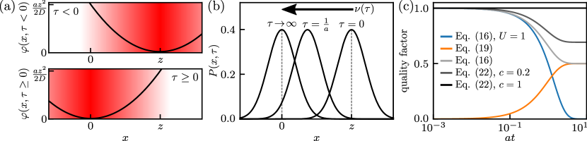
Figure 1: (a) Brownian particle in a one-dimensional harmonic trap with stiffness $a$, $\varphi(x,\tau)=a(x-x^{0}_{\tau})^{2}/2D$ displaced from $x^{0}_{\tau<0}=z$ to $x^{0}_{\tau\geq 0}=0$. Upon being initially equilibrated in $\varphi(x,\tau<0)=a(x-z)^{2}/2D$ (i.e. from the initial condition $p_{0}(x)\propto\exp[-a(x-z)^{2}/2D]$) the particle evolves for $\tau\geq 0$ due to $D\partial_{x}\varphi(x,\tau\geq 0)=ax$ according to $dx_{\tau}=-ax_{\tau}d\tau+\sqrt{2D}dW_{\tau}$ towards an equilibrium $p_{\tau\to\infty}(x)\propto\exp(-ax^{2}/2D)$. (b) Illustration of the evolution of $P(x,\tau)$ for $z=5\sqrt{D/a}$. (c) Quality factors defined as the ratio of right- and left-hand side of the TURs as a function of the dimensionless quantity $at$. All quality factors turn out to be independent of $z,D$ and only depend on $a,t$ through $at$; explicit analytic expressions are given in Note (3). Except for $J_{t}=\int 1\circ dx_{\tau}=x_{t}-x_{0}$ (blue line) we always choose the current defined with $U(\tau)=\nu(\tau)$ and density defined with $V(x,\tau)=-x\nu(\tau)$.

TUR for densities.—We define general, operationally accessible densities (the term “density” is motivated by the analogy to “current” as e.g. in Dieball and Godec (2022a, b); Touchette (2018); Dieball and Godec (2022c))

$$\rho_{t} =\int_{0}^{t}V(\mathbf{x}_{\tau},\tau)d\tau\,,$$

$$\widetilde{\rho}_{t} \equiv\int_{\tau=0}^{\tau=t}\tau\partial_{\tau}V(\mathbf{x}_{\tau},\tau)d\tau\,.$$ (17)

Since in the proof above we did not use the explicit form of $\mathcal{U}$, the density can be treated analogously to $J_{t}$ in Eq. (7) by replacing $\mathcal{U}\to V$ and omitting the $J_{t}^{\rm I}$-term. Analogously to Eqs. (10) and (15) we thus obtain

$$\langle A_{t}(\rho_{t}-\langle\rho_{t}\rangle)\rangle=\langle A_{t}\rho_{t}\rangle=(t\partial_{t}-1)\langle\rho_{t}\rangle-\langle\widetilde{\rho}_{t}\rangle\,,$$ (18)

and analogously to Eq. (11) the transient density-TUR

$$\Sigma_{t}{\rm var}(\rho_{t})\geq 2\left[(t\partial_{t}-1)\langle\rho_{t}\rangle-\langle\widetilde{\rho}_{t}\rangle\right]^{2}.$$ (19)

Note that due to the absence of the $J_{t}^{\rm I}$-term, the right-hand side vanishes in steady-state systems. As in the discussion of Eq. (16) above, Eq. (19) is in some sense contained in the results of Koyuk and Seifert (2020). However, Eq. (19) allows for multidimensional space and multiplicative noise, and does not require a variation in protocol speed.

Improving TURs using correlations.—It has been recently found Dechant and Sasa (2021b) that the steady-state TUR can be eminently improved, and even saturated arbitrarily far from equilibrium, by considering correlations between currents and densities as defined in Eq. (17). To re-derive this sharper version we rewrite Eq. (11) for the observable $J_{t}-c\rho_{t}$ (the constant $c$ is in fact technically redundant since it can be absorbed in the definition of $\rho_{t}$)

$$\frac{\Sigma_{t}}{2}{\rm var}(J_{t}-c\rho_{t}) \geq\left[\langle J_{t}\rangle+\langle A_{t}(J_{t}^{\rm II}-c\rho_{t})\rangle\right]^{2}\,.$$ (20)

Note that ${\rm var}(J_{t}-c\rho_{t})={\rm var}(J_{t})+c^{2}{\rm var}(\rho_{t})-2c\,{\rm cov}(J_{t},\rho_{t})$, where cov denotes the covariance. Using the optimal choice $c={\rm cov}(J_{t},\rho_{t})/{\rm var}(\rho_{t})$ and recalling that for steady-state systems $\langle A_{t}(J_{t}^{\rm II}-c\rho_{t})\rangle=0$, Eq. (20) becomes the NESS correlation-TUR in Dechant and Sasa (2021b)

$$\Sigma_{t}\,{\rm var}(J_{t})\left[1-\chi^{2}_{J\rho}\right]\geq 2\langle J_{t}\rangle^{2},$$

$$\chi^{2}_{J\rho}\equiv\frac{{\rm cov}^{2}(J_{t},\rho_{t})}{{\rm var}(J_{t}){\rm var}(\rho_{t})}\,.$$ (21)

Since $\chi^{2}_{J\rho}\in[0,1]$, Eq. (21) is sharper than Eq. (1) and, as proven in Dechant and Sasa (2021b) and discussed below, for any steady-state system there exist $J_{t},\rho_{t}$ that saturate this inequality.

Our approach allows to generalize this result to transient dynamics by computing $\langle A_{t}(J_{t}^{\rm II}-c\rho_{t})\rangle$ as in Eq. (15) to obtain from Eq. (20) the generalized correlation-TUR

$$\Sigma_{t}\,{\rm var}(J_{t}-c\rho_{t})\geq$$

$$2\left(t\partial_{t}\langle J_{t}\rangle-\langle\widetilde{J}_{t}\rangle-c\left[(t\partial_{t}-1)\langle\rho_{t}\rangle-\langle\widetilde{\rho_{t}}\rangle\right]\right)^{2}.$$ (22)

One could again optimize the left-hand side over $c$ to obtain ${\rm var}(J_{t}-c\rho_{t})={\rm var}(J_{t})\left[1-\chi^{2}_{J\rho}\right]$. However, since here the right-hand side also involves $c$ this may not be the optimal choice. Thus, it is instead practical to keep $c$ general (or absorb it into $\rho_{t}$). The generalized correlation-TUR (22) represents a novel result that sharpens the transient TUR in Eq. (16), and, as we show below and illustrate in Fig. 1, even allows to generally saturate the TUR arbitrarily far from equilibrium.

Saturation of TURs.—For any choice $\mathbf{U}$ in the definition of $J_{t}$ in Eq. (6), the TUR allows to infer a lower bound on the time-accumulated dissipation $\Sigma_{t}$ from $\langle J_{t}\rangle$ and ${\rm var}(J_{t})$ Koyuk and Seifert (2021); Horowitz and Gingrich (2019); Gingrich et al. (2017); Vu et al. (2020); Manikandan et al. (2020); Otsubo et al. (2020); Li et al. (2019); Dieball and Godec (2022a, b). The tighter the inequality, the more precise is the lower bound on $\Sigma_{t}$. It is therefore important to understand when the inequality becomes tight or even saturates, i.e. gives equality.

Due to the simplicity and directness of our proof, we can very well discuss the tightness of the bound based on the single application of the Cauchy-Schwarz inequality. As elaborated in the Appendix, this approach reproduces, and extends beyond, numerous existing results on asymptotic and exact saturation of TURs. Most importantly, choosing $\mathbf{U}(\mathbf{x},\tau)=c^{\prime}[{\mathbf{j}(\mathbf{x}_{\tau},\tau)}/{P(\mathbf{x}_{\tau},\tau)}]\cdot[2\mathbf{D}(\mathbf{x}_{\tau})]^{-1}$ with arbitrary $c^{\prime}$ and $c\rho_{t}=J_{t}^{\rm II}$ (see Eq. (7)) gives $J_{t}-c\rho_{t}=J_{t}^{\rm I}=c^{\prime}A_{t}$ which in turn implies equality in the Cauchy-Schwarz argument leading to the correlation-TURs Eqs. (21) and (22). This directly implies exact saturation of the correlation-TURs which was so far achieved only in the steady-state case Dechant and Sasa (2021b). Our generalization of the correlation-TUR in Eq. (22) for transient systems therefore allows to saturate a TUR arbitrarily far from equilibrium for any $t$ and for general initial conditions and general time-homogeneous dynamics in Eq. (2).
Example.—To illustrate the novel results in Eqs. (16), (19) and (22) and the new insight into the saturation, we provide an explicit example of transient dynamics in Fig. 1, that of a Brownian particle in a one-dimensional harmonic potential $\varphi(x,t)=a(x-x^{0}_{t})^{2}/2D$ displaced from $x^{0}_{\tau<0}=z$ to $x^{0}_{\tau\geq 0}=0$, see Fig. 1(a). This setting, illustrated by the color gradient in Fig. 1a, can easily be realized experimentally using optical tweezers Crocker and Grier (1994); Curtis et al. (2002); Dasgupta et al. (2012). The process features a Gaussian probability density $P(x,\tau)$ with constant variance $D/a$ that moves with a space-independent velocity $\nu(\tau)=j(x,\tau)/P(x,\tau)=-az\exp(-a\tau)$ towards the equilibrium $\propto\exp(-ax^{2}/2D)$, see Fig. 1(b).
To quantify the tightness of the respective TURs we inspect quality factors – the ratio of the right- and left-hand side of the TUR – shown in Fig. 1(c) as a function of the dimensionless quantity $at$.  The blue line represents the transient TUR (16) for the current $J_{t}=x_{t}-x_{0}$ where $U(x,\tau)=1$. Since this $U$ does not feature explicit time-dependence the correction term $\widetilde{J}_{t}$ does not contribute and the transient TUR from the existing literature Dechant and Sasa (2018) applies. The existing (as well as our) results allow varying the spatial dependence of $U$ but we refrain from considering this for simplicity and since it is not necessary for saturation (i.e. $\nu,D$ have no spatial dependence in our example). Due to the novel correction term in Eq. (16) we may choose a time-dependent $U$, and following our discussion of the saturation we choose for all following examples $J_{t}$ with $U(\tau)=c^{\prime}\nu(\tau)/2D=\nu(\tau)$ (the prefactor $c^{\prime}$ is arbitrary as it cancels in quality factor) and the corresponding $\rho_{t}=J_{t}^{II}$, i.e. with $V(x,\tau)=\mathcal{U}(x,\tau)=-axU(\tau)$, see Eq. (7). For this choice we evaluate the transient current [Eq. (16)] and density-TUR [Eq. (19)], see light gray and orange line in Fig. 1(c). Moreover, we evaluate the novel generalized correlation-TUR (22) for $c=0.2$ (dark gray line), where we find that the current TUR is improved by considering correlations with the a density, and for $c=1$ (black line), where we find the expected saturation. This saturation means that the lower bound obtained for $\Sigma_{t}$ from this TUR is exactly $\Sigma_{t}$. Note that this exact saturation requires the knowledge of the details of the dynamics for the choice of $U,V$. However, even with very limited knowledge one can simply consider different guesses or approximations of the optimal $U,V$ and each guess will give a valid lower bound (given sufficient statistics).
Direct route for Markov jump processes.—Beyond overdamped dynamics, one may employ the above direct approach for deriving TURs to Markov jump dynamics on a discrete state-space $\mathcal{N}$ with jump-rates $(r_{xy})_{x,y\in\mathcal{N}}$ and steady-state distribution $(p_{x})_{x\in\mathcal{N}}$. To illustrate this generalization, we here provide the proof of the steady-state TUR (1). Let $\hat{\tau}_{x}$ denote the (random) time spent in state $x$ and $\hat{n}_{xy}$ the (random) number of jumps from $x$ to $y$ in the time interval $[0,t]$. A general time-accumulated current in a jump process is defined with anti-symmetric prefactors $d_{xy}=-d_{yx}$ as the double sum $J\equiv\sum_{x\neq y}d_{xy}\hat{n}_{xy}$. The steady-state dissipation in turn reads $\Sigma\equiv t\sum_{x\neq y}p_{x}r_{xy}\ln[{p_{x}r_{xy}}/{p_{y}r_{yx}}]$. Analogously to $A_{t}$ in Eq. (9) define

$$A \equiv\sum_{x\neq y}\frac{p_{x}r_{xy}-p_{y}r_{yx}}{p_{x}r_{xy}+p_{y}r_{yx}}(\hat{n}_{xy}-\hat{\tau}_{x}r_{xy})\,.$$ (23)

For this choice of $A$ one can check that $\langle A\rangle=0,\ \langle A^{2}\rangle\leq\Sigma/2$, and $\langle AJ\rangle=\langle J\rangle$ (a “direct” proof as above follows by analogy of covariance properties of $\partial_{t}(\hat{n}_{xy}-\hat{\tau}_{x}r_{xy})$ and $\bm{\sigma}(\mathbf{x}_{t})d\mathbf{W}_{t}$, see Note (3) for details) which imply, via the Cauchy-Schwarz inequality, equivalently to Eqs. (10) and (11) the steady-state TUR for Markov jump processes

$$\langle A(J-\langle J\rangle)\rangle=\langle J\rangle\quad\Rightarrow\quad\frac{\Sigma}{2}{\rm var}(J)\geq\langle J\rangle^{2}\,.$$ (24)

A discussion of possible generalizations of this proof beyond steady-state dynamics is given in Note (3).
Conclusion.—Using only stochastic calculus and the well known Cauchy-Schwarz inequality we proved various existing TURs directly from the Langevin equation. This underscores the TUR as an inherent property of overdamped stochastic equations of motion, analogous to quantum-mechanical uncertainty relations. Moreover, by including current-density correlations we derived a new sharpened TUR for transient dynamics. Based on our simple and more direct proof we were able to systematically explore conditions under which TURs saturate. The new equality (10) is mathematically even stronger than TUR (11). Therefore it allows to derive further bounds, e.g. by applying Hölder’s instead of the Cauchy-Schwarz inequality which, however, may not yield operationally accessible quantities. Our approach may allow for generalizations to systems with time-dependent driving (see e.g. Koyuk and Seifert (2020)) which, however, are not expected to follow anymore directly from a single equation of motion. The novel correction term for currents with explicit time dependence as well as the new transient correlation-TUR and its saturation are expected to equally apply to Markov jump processes by generalizing the approach illustrated in Eqs. (23) and (24).

Acknowledgments.—We thank David Hartich for insightful suggestions and critical reading of the manuscript. Financial support from Studienstiftung des Deutschen Volkes (to C. D.) and the German Research Foundation (DFG) through the Emmy Noether Program GO 2762/1-2 (to A. G.) is gratefully acknowledged.

Appendix: Saturation of TURs.—Thanks to the directness of our proof, we only need to discuss the tightness based on the step from Eq. (10) to Eq. (11) where we applied the Cauchy-Schwarz inequality $\langle A_{t}(J_{t}-\langle J_{t}\rangle)\rangle^{2}\leq\langle A_{t}^{2}\rangle{\rm var}(J_{t})$ to the exact Eq. (10). Thus, the closer $A_{t}$ and $J_{t}-\langle J_{t}\rangle$ are to being linearly dependent (recall that the Cauchy-Schwarz inequality measures the angle $\varphi$ between two vectors $(\vec{x}\cdot\vec{y})^{2}=\vec{x}^{\,2}\vec{y}^{\,2}\cos^{2}(\varphi)\leq\vec{x}^{\,2}\vec{y}^{\,2}$), the tighter the TUR, with saturation for $J_{t}-\langle J_{t}\rangle=c^{\prime}A_{t}$ for some constant $c^{\prime}$. Therefore, the TUR is expected to be tightest for the choice $\mathbf{U}(\mathbf{x},\tau)=c^{\prime}[{\mathbf{j}(\mathbf{x}_{\tau},\tau)}/{P(\mathbf{x}_{\tau},\tau)}]\cdot[2\mathbf{D}(\mathbf{x}_{\tau})]^{-1}$ for which $J_{t}^{\rm I}=c^{\prime}A_{t}$ (see Eq. (7)). Note that for NESS this $\mathbf{U}$ becomes time-independent with $\mathbf{j}_{\rm s}(\mathbf{x})/P_{\rm s}(\mathbf{x})$. This choice is known to saturate the original TUR in Eq. (1) in the near-equilibrium limit Pigolotti et al. (2017). However, since the full $J_{t}=J_{t}^{\rm I}+J_{t}^{\rm II}$ current cannot be chosen to exactly agree with $c^{\prime}A_{t}$, equality is generally not reached.

The original TUR (1) with this choice of $\mathbf{U}(\mathbf{x},\tau)$ was also found to saturate in the short-time limit $t\to 0$ Manikandan et al. (2020); Otsubo et al. (2020). This result is in turn reproduced with our approach by noting that $J_{t}^{\rm I}=c^{\prime}A_{t}$ and $\langle A_{t}J_{t}^{\rm II}\rangle=0$ give $\langle A_{t}(J_{t}-\langle J_{t}\rangle)\rangle^{2}=\langle A_{t}J_{t}^{\rm I}\rangle^{2}=\langle A_{t}^{2}\rangle\langle{J_{t}^{\rm I}}^{2}\rangle$, and in the limit $t\to 0$ the integrals in Eq. (7) asymptotically scale like a single time-step, such that $\langle{J_{t}^{\rm I}}^{2}\rangle\sim(\mathbf{W}_{t}-\mathbf{W}_{0})^{2}\sim t$ dominates all $\sim t^{3/2},\,\sim t^{2}$ contributions in ${\rm var}(J_{t})$. In turn, $\langle{J_{t}^{\rm I}}^{2}\rangle\overset{t\to 0}{\to}{\rm var}(J_{t})$ which yields $\langle A_{t}(J_{t}-\langle J_{t}\rangle)\rangle^{2}\overset{t\to 0}{\to}\langle A_{t}^{2}\rangle{\rm var}(J_{t})$. Thus, the Cauchy-Schwarz step from the equality (10) to the inequality (11) saturates as $t\to 0$, in turn implying that the TUR saturates.

More recently it was also found that including correlations (see Eq. (21) and Ref. Dechant and Sasa (2021b)) allows to saturate a sharpened TUR for steady-state systems arbitrarily far from equilibrium for any $t$, again for the same choice $\mathbf{U}(\mathbf{x},\tau)$ as above. Since our re-derivation of the NESS correlation-TUR in Eq. (21) applied the Cauchy-Schwarz inequality to $A_{t}$ and $J_{t}-c\rho_{t}$ we see that choosing $c\rho_{t}=J_{t}^{\rm II}$ yields $J_{t}-c\rho_{t}=J_{t}^{\rm I}=c^{\prime}A_{t}$, such that the application of the Cauchy-Schwarz inequality becomes an equality. That is, the correlation-TUR (21) for this choice of $J_{t}$ and $\rho_{t}$ is generally saturated. Notably, this powerful result follows very naturally from the direct proof presented here.

Our generalization of the correlation-TUR in Eq. (22) for transient systems even allows to saturate a TUR (arbitrarily far from equilibrium for any $t$ and) for general initial conditions and general time-homogeneous dynamics in Eq. (2). This result is strong but obvious, since as for the NESS correlation-TUR we can choose $J_{t}$ and $\rho_{t}$ such that $J_{t}-c\rho_{t}=c^{\prime}A_{t}$. Note that it is here crucial that we allowed for an explicit time-dependence in $\mathbf{U}$ and $V$, i.e. that we found new correction terms (terms with tilde in Eqs. (16), (19) and (22)).

In this Supplementary Material we provide a detailed analysis of the quality (i.e. sharpness) of the distinct versions of thermodynamic uncertainty relation (TUR) applied to the transient example shown in the Letter as well as counterexamples underscoring the necessity of the novel versions of the TUR. Moreover, we provide technical details on the direct proof of the TUR as well as a perspective on the extension of the direct proof to Markov-jump processes.

I Quality of TURs for displaced harmonic trap

In the following we derive the quality factors (i.e. the sharpness of the various TURs) shown in Fig. 1 in the Letter. Consider one-dimensional Brownian motion in a parabolic potential (i.e. a Langevin equation with linear force; known as the Ornstein-Uhlenbeck process) Gardiner (1985) with a Gaussian initial condition $x_{0}$ [we denote a a normal distribution by $\mathcal{N}({\rm mean,\,variance})$],

$$dx_{\tau} =-ax_{\tau}d\tau+\sqrt{2D}dW_{\tau}\,,\qquad x_{0}\sim\mathcal{N}(z,\sigma_{0}^{2})\,.$$ (S1)

Even though this process approaches an equilibrium steady state, for finite times it features transient dynamics if $x_{0}$ is not sampled from the steady-state distribution. For any Gaussian initial condition this process is Gaussian Gardiner (1985). Therefore, the mean and the variance completely determine the distribution of $x_{\tau}$. The harmonic potential and the Gaussian initial condition can be realized experimentally by optical tweezers. The mean, variance and covariance are simply obtained as (see e.g. Appendix F in Ref. Dieball et al. (2022))

$$\langle x_{\tau}\rangle =z\mathrm{e}^{-a\tau}\,,$$

$${\rm var}(x_{\tau}) \equiv\langle x_{\tau}^{2}\rangle-\langle x_{\tau}\rangle^{2}=\frac{D}{a}\left(1-\mathrm{e}^{-2a\tau}\right)+\sigma_{0}^{2}\mathrm{e}^{-2a\tau}\,,$$

$${\rm For\ }\tau\geq\tau^{\prime}\colon\quad{\rm cov}(x_{\tau},x_{\tau^{\prime}}) \equiv\langle x_{\tau}x_{\tau^{\prime}}\rangle-\langle x_{\tau}\rangle\langle x_{\tau^{\prime}}\rangle=\mathrm{e}^{-a(\tau-\tau^{\prime})}{\rm var}(x_{\tau^{\prime}})\,.$$ (S2)

The Gaussian probability density $P(x,\tau)$ given the initial condition in Eq. (S1) accordingly reads

$$P(x,\tau) =\sqrt{\frac{1}{2\pi{\rm var}(x_{\tau})}}\exp\left[-\frac{(x-z\mathrm{e}^{-a\tau})^{2}}{2{\rm var}(x_{\tau})}\right]\,.$$ (S3)

The local mean velocity $\nu(x,\tau)\equiv j(x,\tau)/P(x,\tau)$ with current $j(x,\tau)\equiv(-ax-D\partial_{x})P(x,\tau)$ reads

$$\nu(x,\tau)=-ax+D(x-z\mathrm{e}^{-a\tau})/{\rm var}(x_{\tau})\,.$$ (S4)

For this example we consider the simple case $\sigma_{0}^{2}=D/a$, i.e. we start in the steady-state variance (but as long as $z\neq 0$ not in the steady-state distribution; can be realized by equilibration with optical tweezers at $x=z$ at times $\tau<0$ and an equally stiff optical trap at position $x=0$ at times $\tau\geq 0$), for which we obtain the simplified expressions

$${\rm var}(x_{\tau}) =D/a\,,$$

$${\rm For\ }\tau\geq\tau^{\prime}\colon\quad{\rm cov}(x_{\tau},x_{\tau^{\prime}}) =\mathrm{e}^{-a(\tau-\tau^{\prime})}D/a\,,$$

$$\nu(x,\tau) =-az\mathrm{e}^{-a\tau}\,.$$ (S5)

For this initial condition, $P(x,\tau)$ corresponds to a Gaussian distribution of constant variance with mean value $z\mathrm{e}^{-a\tau}$ drifting from $z$ to $0$. Since only the mean changes (but the distribution around the mean remains invariant), the local mean velocity $\nu(x,\tau)$ is independent of $x$ [and in fact given by the velocity of the mean $\nu(x,\tau)=\partial_{\tau}\langle x_{\tau}\rangle$]. This easily allows to compute the time-accumulated dissipation

$$\Sigma_{t}=D^{-1}\int_{0}^{t}d\tau\int dx\langle\nu(x_{\tau},\tau)\rangle^{2}=\frac{a^{2}z^{2}}{D}\int_{0}^{t}d\tau\mathrm{e}^{-2a\tau}=\frac{az^{2}}{2D}(1-\mathrm{e}^{-2at})\,.$$ (S6)

Apart from $\Sigma_{t}$ the TURs contain first and second moments of (generalized) currents and densities that we derive for some examples below. Recall the definition of a generalized current (here in one-dimensional space)

$$J_{t} \equiv\int_{\tau=0}^{\tau=t}U(x_{\tau},\tau)\circ dx_{\tau}\,.$$ (S7)

For simplicity (and since in our example the mean velocity $\nu(\tau)$ is space-independent) we consider only currents without explicit space dependence, i.e. only $U(x_{\tau},\tau)=U(\tau)$. In this case there is no difference between the Stratonovich and Itô interpretation of the integral, i.e. $J_{t}=\int_{\tau=0}^{\tau=t}U(\tau)dx_{\tau}$.

I.1 Current without explicit time-dependence

For the simplest case of $U(x,\tau)=1$ we have the displacement current (denote this choice of current by $J_{t}^{x}$)

$$J_{t}^{x}\equiv\int_{\tau=0}^{\tau=t}1\circ dx_{\tau}=x_{t}-x_{0}\,.$$ (S8)

From Eq. (S5) we obtain

$$\langle J_{t}\rangle =-z(1-\mathrm{e}^{-at})\,,\qquad t\partial_{t}\langle J_{t}\rangle=-zat\mathrm{e}^{-at}\,,$$

$${\rm var}(J_{t}) ={\rm var}(x_{t})+{\rm var}(x_{0})-2{\rm cov}(x_{t},x_{0})=\frac{2D}{a}(1-\mathrm{e}^{-at})\,.$$ (S9)

Recalling the expression for the dissipation Eq. (S6) the transient TUR $\Sigma_{t}{\rm var}(J_{t})\geq 2[t\partial_{t}\langle J_{t}\rangle]^{2}$ in this example reads $\frac{az^{2}}{2D}(1-\mathrm{e}^{-2at})\frac{2D}{a}(1-\mathrm{e}^{-at})\geq 2(zat)^{2}\mathrm{e}^{-2at}$ such that the quality factor $Q_{x}\in[0,1]$ (ratio of right-hand side and left-hand side; measures sharpness of the inequality) in this example becomes

$$Q_{x}\equiv\frac{2[t\partial_{t}\langle J_{t}\rangle]^{2}}{\Sigma_{t}{\rm var}(J_{t})}=\frac{2(at)^{2}\mathrm{e}^{-2at}}{\left(1-\mathrm{e}^{-2at}\right)\left(1-\mathrm{e}^{-at}\right)}\,.$$ (S10)

Note that $Q_{x}$ is independent of $z$ and $D$ and only depends on the dimensionless quantity $at$. For large values $at\to\infty$ we have $Q_{x}\to 0$, see also Fig. 1 in the Letter.

I.2 Currents with explicit time-dependence

Saturating a TUR (i.e. obtaining the true dissipation as the lower bound inferred by the TUR) can be achieved for the transient correlation-TUR [Eq. (22) in the Letter] by choosing $\mathbf{U}(\mathbf{x},\tau)=c^{\prime}[{\mathbf{j}(\mathbf{x}_{\tau},\tau)}/{P(\mathbf{x}_{\tau},\tau)}]\cdot[2\mathbf{D}(\mathbf{x}_{\tau})]^{-1}$, and the corresponding density $\rho_{t}=\int_{0}^{t}\big{[}\mathbf{U}(\mathbf{x}_{\tau},\tau)\cdot\mathbf{F}(\mathbf{x}_{\tau})+\nabla\cdot\left[\mathbf{D}(\mathbf{x}_{\tau})\mathbf{U}(\mathbf{x}_{\tau},\tau)\right]\big{]}d\tau$. For this example, the respective current and density (denote this choice by superscript $\nu$) read (Stratonovich convention irrelevant since $\partial_{x}U(x,\tau)=0$ here)

$$J_{t}^{\nu} \equiv\frac{c^{\prime}}{2D}\int_{\tau=0}^{\tau=t}\nu(\tau)dx_{\tau}\,,\qquad\rho_{t}^{\nu}\equiv\frac{-ac^{\prime}}{2D}\int_{0}^{t}x_{\tau}\nu(\tau)d\tau\,,$$ (S11)

with $\nu(\tau)=-az\mathrm{e}^{-a\tau}$, see Eq. (S5). The prefactor $c^{\prime}$ will equally appear on both sides of the TURs and therefore not change the quality factors. One may set $c^{\prime}=2D$ as done in the Letter, but here we keep it general. Plugging in $dx_{\tau}$ from Eq. (S1) we calculate

$$\langle J_{t}^{\nu}\rangle =\frac{c^{\prime}}{2D}\int_{0}^{t}\nu(\tau)\langle-ax_{\tau}\rangle d\tau=\frac{-azc^{\prime}}{2D}\int_{0}^{t}\nu(\tau)\mathrm{e}^{-a\tau}d\tau=\frac{(az)^{2}c^{\prime}}{2D}\int_{0}^{t}\mathrm{e}^{-2a\tau}d\tau=\frac{az^{2}c^{\prime}}{4D}(1-\mathrm{e}^{-2at})\,,$$

$$t\partial_{t}\langle J_{t}^{\nu}\rangle =t\frac{(az)^{2}c^{\prime}}{2D}\mathrm{e}^{-2at}\,,\qquad\langle\rho_{t}^{\nu}\rangle=\langle J_{t}^{\nu}\rangle\,,\qquad t\partial_{t}\langle\rho_{t}^{\nu}\rangle=t\partial_{t}\langle J_{t}^{\nu}\rangle\,.$$ (S12)

The auxiliary current $\widetilde{J}_{t}\equiv\int_{\tau=0}^{\tau=t}\tau\partial_{\tau}U(x_{\tau},\tau)\circ dx_{\tau}$ and density $\widetilde{\rho}_{t}$ have due to $\tau\partial_{\tau}\nu(\tau)=-a\tau\nu(\tau)$ the mean

$$\langle\widetilde{\rho}_{t}^{\nu}\rangle=\langle\widetilde{J}_{t}^{\nu}\rangle=\frac{-a(az)^{2}c^{\prime}}{2D}\int_{0}^{t}\tau\mathrm{e}^{-2a\tau}d\tau=\frac{-a(az)^{2}c^{\prime}}{2D}\,\frac{1-\mathrm{e}^{-2at}(1+2at)}{4a^{2}}=\frac{-az^{2}c^{\prime}}{8D}[1-(1+2at)\mathrm{e}^{-2at}]\,.$$ (S13)

For the variance split $J_{t}^{\nu}=J_{t}^{\rm I}+J_{t}^{\rm II}$ with

$$J_{t}^{\rm I} =\frac{c^{\prime}}{2D}\int_{\tau=0}^{\tau=t}\nu(\tau)\sqrt{2D}dW_{\tau}\,,\qquad J_{t}^{\rm II}=\rho_{t}^{\nu}\,,$$ (S14)

and compute

$${\rm var}(\rho_{t}^{\nu}) ={\rm var}(J_{t}^{\rm II})=\frac{a^{2}c^{\prime 2}}{4D^{2}}\left\langle\left(\int_{0}^{t}\nu(\tau)(\mathbf{x}_{\tau}-\langle\mathbf{x}_{\tau}\rangle)d\tau\right)^{2}\right\rangle$$

$$=\frac{a^{2}c^{\prime 2}}{4D^{2}}2\int_{0}^{t}d\tau\int_{0}^{\tau}d\tau^{\prime}\,\nu(\tau)\nu(\tau^{\prime}){\rm cov}(x_{\tau},x_{\tau^{\prime}})$$

$$=\frac{a^{3}z^{2}c^{\prime 2}}{2D}\int_{0}^{t}d\tau\int_{0}^{\tau}d\tau^{\prime}\mathrm{e}^{-a(\tau+\tau^{\prime})}\mathrm{e}^{-a(\tau-\tau^{\prime})}$$

$$=\frac{a^{3}z^{2}c^{\prime 2}}{2D}\int_{0}^{t}d\tau\tau\mathrm{e}^{-2a\tau}$$

$$=\frac{c^{\prime 2}az^{2}}{8D}\left[1-(1+2at)\mathrm{e}^{-2at}\right]\,.$$ (S15)

The cross terms are given by the non-trivial correlations of $dW_{\tau}$ and $d\tau^{\prime}$ integrals exactly as Eq. (13) in the Letter, in this example with $\mathcal{U}(x^{\prime},\tau^{\prime})=-ax^{\prime}\nu(\tau^{\prime})c^{\prime}/(2D)$, such that

$$\langle J_{t}^{\rm I}J_{t}^{\rm II}\rangle =-\int_{0}^{t}d\tau^{\prime}\int dx^{\prime}\mathcal{U}(x^{\prime},\tau^{\prime})\int_{0}^{t}d\tau\mathbbm{1}_{\tau<\tau^{\prime}}\int dxP(x^{\prime},\tau^{\prime}|x,\tau)\partial_{x}c^{\prime}\nu(\tau)P(x,\tau)$$

$$=\frac{c^{\prime 2}a}{2D}\int_{0}^{t}d\tau^{\prime}\int_{0}^{\tau^{\prime}}d\tau\nu(\tau)\nu(\tau^{\prime})\int dx^{\prime}x^{\prime}P(x^{\prime},\tau^{\prime}|x,\tau)\partial_{x}P(x,\tau)\,.$$ (S16)

From Eq. (S3) we get

$$\partial_{x}P(x,\tau)=-(x-z\mathrm{e}^{-a\tau})P(x,\tau)/{\rm var}(x_{\tau})=-\frac{a}{D}(x-z\mathrm{e}^{-a\tau})P(x,\tau)\,.$$ (S17)

Hence using $z\mathrm{e}^{-a\tau}=\langle x_{\tau}\rangle$ and $\langle\langle x_{\tau^{\prime}}\rangle(x_{\tau}-\langle x_{\tau}\rangle)\rangle=0$ we obtain

$$\langle J_{t}^{\rm I}J_{t}^{\rm II}\rangle =-\frac{c^{\prime 2}a^{2}}{2D^{2}}\int_{0}^{t}d\tau^{\prime}\int_{0}^{\tau^{\prime}}d\tau\nu(\tau)\nu(\tau^{\prime})\int dx^{\prime}(x-z\mathrm{e}^{-a\tau})x^{\prime}P(x^{\prime},\tau^{\prime};x,\tau)$$

$$=-\frac{c^{\prime 2}a^{2}}{2D^{2}}\int_{0}^{t}d\tau^{\prime}\int_{0}^{\tau^{\prime}}d\tau\nu(\tau)\nu(\tau^{\prime})\langle x_{\tau^{\prime}}(x_{\tau}-\langle x_{\tau}\rangle)\rangle$$

$$=-\frac{c^{\prime 2}a^{2}}{2D^{2}}\int_{0}^{t}d\tau^{\prime}\int_{0}^{\tau^{\prime}}d\tau\nu(\tau)\nu(\tau^{\prime}){\rm cov}(x_{\tau},x_{\tau^{\prime}})\,.$$ (S18)

Comparison with the third line in Eq. (S15) yields

$$\langle J_{t}^{\rm I}J_{t}^{\rm II}\rangle=-{\rm var}(\rho_{t}^{\nu})\,.$$ (S19)

Therefore from $J_{t}^{\nu}=J_{t}^{\rm I}+J_{t}^{\rm II}$ with $\langle J_{t}^{\rm I}\rangle=0$ we obtain

$${\rm var}(J_{t}^{\nu}) =\langle{J_{t}^{\rm I}}^{2}\rangle+{\rm var}(J_{t}^{\rm II})+2\langle J_{t}^{\rm I}J_{t}^{\rm II}\rangle=\frac{c^{\prime 2}}{2}\Sigma_{t}-{\rm var}(\rho_{t}^{\nu})\overset{\rm Eqs.~{}\eqref{SM Sigma},\eqref{SM var rho nu}}{=}\frac{c^{\prime 2}az^{2}}{8D}\left[1+(2at-1)\mathrm{e}^{-2at}\right]\,.$$ (S20)

Since $\rho_{t}^{\nu}=J_{t}^{\rm II}$ and $\langle J_{t}^{\rm I}\rangle=0$, Eq. (S19) implies

$${\rm cov}(J_{t}^{\nu},\rho_{t}^{\nu})={\rm cov}(J_{t}^{\rm I}+J_{t}^{\rm II},J_{t}^{\rm II})=\langle J_{t}^{\rm I}J_{t}^{\rm II}\rangle+{\rm var}(J_{t}^{\rm II})=0\,,$$ (S21)

which gives

$${\rm var}(J_{t}^{\nu}-c\rho_{t}^{\nu}) ={\rm var}(J_{t}^{\nu})+c^{2}{\rm var}(\rho_{t}^{\nu})$$

$$=\frac{c^{\prime 2}az^{2}}{8D}\Big{(}1+(2at-1)\mathrm{e}^{-2at}+c^{2}\left[1-(1+2at)\mathrm{e}^{-2at}\right]\Big{)}\,.$$ (S22)

We now have evaluated all expressions entering the various transient TURs for the current $J_{t}^{\nu}$ and density $\rho_{t}^{\nu}$. The quality factors (ratios of right- and left-hand side) $Q_{J}$ for the transient TUR $\Sigma_{t}{\rm var}(J_{t})\geq 2[t\partial_{t}\langle J_{t}\rangle-\langle\widetilde{J}_{t}\rangle]^{2}$ [Eq. (16) in the Letter], $Q_{\rho}$ for the transient density-TUR $\Sigma_{t}{\rm var}(\rho_{t})\geq 2[(t\partial_{t}-1)\langle\rho_{t}\rangle-\langle\widetilde{\rho}_{t}\rangle]^{2}$ [Eq. (19) in the Letter], and $Q_{C}(c)$ (function of $c$) for the transient correlation-TUR $\Sigma_{t}{\rm var}(J_{t}-c\rho_{t})\geq 2(t\partial_{t}\langle J_{t}\rangle-\langle\widetilde{J}_{t}\rangle-c[(t\partial_{t}-1)\langle\rho_{t}\rangle-\langle\widetilde{\rho_{t}}\rangle])^{2}$ [Eq. (22) in the Letter] after straightforward simplifications read

$$Q_{J} =\frac{1-(1-2at)\mathrm{e}^{-2at}}{2(1-\mathrm{e}^{-2at})}\,,$$

$$Q_{\rho} =\frac{1-(1+2at)\mathrm{e}^{-2at}}{2(1-\mathrm{e}^{-2at})}\,,$$

$$Q_{C}(c) =\frac{\left[(1+c)(1-\mathrm{e}^{-2at})+(1-c)2at\mathrm{e}^{-2at}\right]^{2}}{2(1-\mathrm{e}^{-2at})\left[(1+c^{2})(1-\mathrm{e}^{-2at})+(1-c^{2})2at\mathrm{e}^{-2at}\right]}\,,$$

$$Q_{C}(1) =1\,.$$ (S23)

These quality factors along with $Q_{x}$ in Eq. (S10) are depicted in Fig. 1 in the Letter. They only depend on the dimensionless quantity $at$ but not on other parameters of the process.

Opposed to $Q_{x}$ in Eq. (S10) these quality factors approach non-zero values as $at\to\infty$, namely $Q_{J}\to 1/2$, $Q_{\rho}\to 1/2$, $Q_{C}(c)\to(1+c)^{2}/2(1+c^{2})$. Interestingly, for this special case the current and density quality factors add up to one, $Q_{J}+Q_{\rho}=1$. While $\lim_{at\to 0}Q_{J}=1$ [as expected in general for such choice of current (see “saturation”-paragraph in the Letter)], we have $\lim_{at\to 0}Q_{\rho}=0$. This is because $at\to 0$ corresponds to the steady-state limit where the density-TUR becomes the trivial $\Sigma_{t}{\rm var}(\rho_{t})\geq 0$.

Recall that ${\rm cov}(J_{t}^{\nu},\rho_{t}^{\nu})=0$ [see Eq. (S21)]. We now see that the choice $c={\rm cov}(J_{t},\rho_{t})/{\rm var}(\rho_{t})$, that is optimal in steady-state dynamics (see Letter), here gives $c=0$ although $c=1$ is optimal, see Eq. (S23). As mentioned in the Letter, this arises because $c=0$ only optimizes the left-hand side of the corelation-TUR [also seen from Eq. (S21)] but in the generalized (i.e. transient) correlation-TUR the right-hand side also depends on $c$.

II Counterexamples

We showed that the TUR for transient dynamics [Eq. (16) in the Letter] reads $\Sigma_{t}{\rm var}(J_{t})\geq 2[t\partial_{t}\langle J_{t}\rangle-\langle\widetilde{J}_{t}\rangle]^{2}$ and thus contains the correction term $-\langle\widetilde{J}_{t}\rangle$ which contributes if $\mathbf{U}(\mathbf{x},\tau)$ in the current $J_{t}\equiv\int_{\tau=0}^{\tau=t}U(\mathbf{x}_{\tau},\tau)\circ dx_{\tau}$ depends on time $\tau$. Based on the setting in the previous section (and Fig. 1 in the Letter) we here give an explicit counterexample for the TUR without the correction term, i.e. an example where $\Sigma_{t}{\rm var}(J_{t})<2\left[t\partial_{t}\langle J_{t}\rangle\right]^{2}$. This shows that the correction term $-\langle\widetilde{J}_{t}\rangle$ is indeed necessary, and that the result in Eq. (16) in the Letter is valid for a broader class of systems than existing literature Dechant and Sasa (2018) by allowing explicit time-dependence in $\mathbf{U}(\mathbf{x}_{\tau},\tau)$. In addition we also provide a counterexample to show that the NESS TUR $\Sigma{\rm var}(J_{t})\geq 2\langle J_{t}\rangle^{2}$ does not hold in this transient system. Both counterexamples are shown in Fig. S1 and the derivations of the respective terms are shown below.

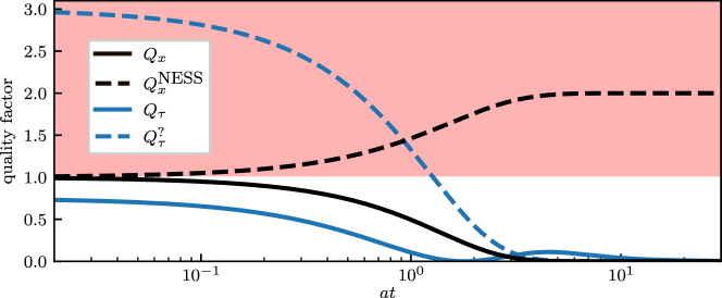
Figure S1: Quality factors for the displaced harmonic trap for currents $J_{t}^{x}\equiv\int_{\tau=0}^{\tau=t}1\circ dx_{\tau}=x_{t}-x_{0}$ (black) and $J_{t}^{\tau}\equiv\int_{\tau=0}^{\tau=t}\tau\circ dx_{\tau}$ (blue). Quality factors $Q_{x,\tau}\equiv 2[t\partial_{t}\langle J_{t}^{x,\tau}\rangle-\langle\widetilde{J}_{t}^{x,\tau}\rangle]^{2}/\Sigma_{t}{\rm var}(J_{t}^{x,\tau})\leq 1$, see Eqs. (S10) and (S28), for the transient TUR [Eq. (16) in the Letter] are shown by solid lines. The dashed black line $Q_{x}^{\rm NESS}\equiv 2\langle J_{t}^{x}\rangle^{2}/\Sigma_{t}{\rm var}(J_{t}^{x})$, see Eq. (S29), and dashed blue line $Q_{\tau}^{?}\equiv 2[t\partial_{t}\langle J_{t}^{\tau}\rangle]^{2}/\Sigma_{t}{\rm var}(J_{t}^{\tau})$, see Eq. (S27), intersect the forbidden region $Q>1$ (red background) which shows that the NESS TUR and the transient TUR without the correction $-\langle\widetilde{J}_{t}\rangle$ term are not generally valid for transient systems.

To find an example for which $2\left[t\partial_{t}\langle J_{t}\rangle\right]^{2}>\Sigma_{t}{\rm var}(J_{t})$, we note [recalling Eq. (8) in the Letter, $\langle J_{t}\rangle=\int_{0}^{t}d\tau\int d\mathbf{x}\mathbf{U}(\mathbf{x},\tau)\cdot\mathbf{j}(\mathbf{x},\tau)$] that the term $t\partial_{t}\langle J_{t}\rangle=t\int d\mathbf{x}\mathbf{U}(\mathbf{x},t)\cdot\mathbf{j}(\mathbf{x},t)$ only involves $\mathbf{U}(\mathbf{x},t)$ at the final time but not at any $\tau<t$. In contrast, $\Sigma_{t}$ is independent of the choice of $\mathbf{U}$ and ${\rm var}(J_{t})$ involves $\mathbf{U}(\mathbf{x},\tau)$ at all times. Therefore, examples for $2\left[t\partial_{t}\langle J_{t}\rangle\right]^{2}>\Sigma_{t}{\rm var}(J_{t})$ can be found by making $\mathbf{U}(\mathbf{x},t)$ large compared to $\mathbf{U}(\mathbf{x},\tau)$ at $\tau<t$.

We now give an explicit example by choosing a current $J_{t}^{\tau}$ with linear time-dependence in $U(x,\tau)=\tau$ (here one-dimensional),

$$J_{t}^{\tau} \equiv\int_{\tau=0}^{\tau=t}\tau\circ dx_{\tau}\,.$$ (S24)

Note that due to $\partial_{x}U(x,\tau)=0$ there is no difference between Stratonovich and Itô integration. We calculate

$$\langle J_{t}^{\tau}\rangle =\int_{0}^{t}\tau\langle-ax_{\tau}\rangle d\tau=-az\int_{0}^{t}\tau\mathrm{e}^{-a\tau}d\tau=-\frac{z}{a}\left[1-\mathrm{e}^{-at}(1+at)\right]\,,$$

$$t\partial_{t}\langle J_{t}^{\tau}\rangle =\frac{zt}{a}\left[-a(1+at)+a\right]\mathrm{e}^{-at}=-zat^{2}\mathrm{e}^{-at}\,.$$ (S25)

For the variance compute analogously to the lines leading to Eq. (S20) [with cov from Eq. (S5)]

$${\rm var}(J_{t}^{\tau}) =2D\int_{0}^{t}d\tau\,\tau^{2}-a^{2}\int_{0}^{t}d\tau\int_{0}^{t}d\tau^{\prime}\,\tau\tau^{\prime}{\rm cov}(x_{\tau},x_{\tau^{\prime}})$$

$$=2\frac{D}{a^{3}}\left(\frac{a^{3}t^{3}}{3}-\frac{1}{6}\left[a^{2}t^{2}(2at-3)-6\mathrm{e}^{-at}(1+at)+6\right]\right)$$

$$=\frac{D}{a^{3}}\left[a^{2}t^{2}+2\mathrm{e}^{-at}(1+at)-2\right]\,.$$ (S26)

Since the dissipation $\Sigma_{t}$ does not depend on the choice of $J_{t},U$, it is still given by Eq. (S6). The quality factor $Q_{\tau}^{?}$ for the TUR $\Sigma_{t}{\rm var}(J_{t})\geq 2\left[t\partial_{t}\langle J_{t}\rangle\right]^{2}$ that would hold in the absence of explicit time-dependence in $U$ [Eq. (16) in the Letter for $\langle\widetilde{J}_{t}\rangle=0$; see also Ref. Dechant and Sasa (2018)] reads

$$Q_{\tau}^{?} =\frac{4a^{4}t^{4}\mathrm{e}^{-2at}}{(1-\mathrm{e}^{-2at})\left[a^{2}t^{2}+2\mathrm{e}^{-at}(1+at)-2\right]}\,.$$ (S27)

Thus we see that as the other quality factors in Eqs. (S10) and (S23), $Q_{\tau}^{?}$ only depends on the quantity $at$. In Fig. S1 we see that $Q_{\tau}^{?}>1$ for small values of $at$ which breaks the TUR $\Sigma_{t}{\rm var}(J_{t})\geq 2\left[t\partial_{t}\langle J_{t}\rangle\right]^{2}$, i.e. this example shows that the correction term $-\langle\widetilde{J}_{t}\rangle$ in the TUR $\Sigma_{t}{\rm var}(J_{t})\geq 2[t\partial_{t}\langle J_{t}\rangle-\langle\widetilde{J}_{t}\rangle]^{2}$ [Eq. (16) in the Letter] is necessary for general validity for currents with explicitly time-dependent $\mathbf{U}$.

For comparison we also give the correct quality factor $Q_{\tau}$ for the transient TUR [Eq. (16) in the Letter] including the correction term $-\langle\widetilde{J}_{t}\rangle$. Since $\tau\partial_{\tau}\tau=\tau$ we have $\widetilde{J}_{t}=J_{t}$ such that the correct quality factor using Eq. (S25) reads

$$Q_{\tau} =\frac{2\left(-zat^{2}\mathrm{e}^{-at}+\frac{z}{a}\left[1-\mathrm{e}^{-at}(1+at)\right]\right)^{2}}{\frac{az^{2}}{2D}(1-\mathrm{e}^{-2at})\frac{D}{a^{3}}\left[a^{2}t^{2}+2\mathrm{e}^{-at}(1+at)-2\right]}$$

$$=\frac{4\left[1-\mathrm{e}^{-at}(1+at+a^{2}t^{2})\right]^{2}}{(1-\mathrm{e}^{-2at})\left[a^{2}t^{2}+2\mathrm{e}^{-at}(1+at)-2\right]}\,.$$ (S28)

To give a counterexample that shows that NESS TUR $\Sigma_{t}{\rm var}(J_{t})\geq 2\langle J_{t}\rangle^{2}$ breaks down for this transient system, consider the current $J_{t}^{x}=x_{t}-x_{0}$ as in Eq. (S8). The quality factor for this example follows from Eq. (S9),

$$Q_{x}^{\rm NESS} =\frac{2z^{2}(1-\mathrm{e}^{-at})^{2}}{\frac{az^{2}}{2D}(1-\mathrm{e}^{-2at})\frac{2D}{a}(1-\mathrm{e}^{-at})}=\frac{2(1-\mathrm{e}^{-at})}{1-\mathrm{e}^{-2at}}\,.$$ (S29)

Note that for any $y\in[0,1)$ the inequality $(1-y)^{2}>0$ implies $2(1-y)>1-y^{2}$. Thus we have for any value $at>0$ that $Q_{x}^{\rm NESS}>1$, see also Fig. S1. This provides (for any $at>0$) a counterexample against the NESS TUR, i.e. as expected the NESS TUR does not hold for transient dynamics.

III Detailed derivation of $\langle A_{t}^{2}\rangle=\Sigma_{t}/2$

Recall the “educated guess” [Eq. (9) in the Letter]

$$A_{t} \equiv\int_{\tau=0}^{\tau=t}\mathbf{a}(\mathbf{x}_{\tau},\tau)^{T}d\mathbf{W}_{\tau}\,,$$

$$\mathbf{a}(\mathbf{x}_{\tau},\tau)^{T} \equiv\frac{\mathbf{j}(\mathbf{x}_{\tau},\tau)^{T}}{P(\mathbf{x}_{\tau},\tau)}[2\mathbf{D}(\mathbf{x}_{\tau})]^{-1}\bm{\sigma}(\mathbf{x}_{\tau})\,,$$

$$\mathbf{a}(\mathbf{x}_{\tau},\tau) =\bm{\sigma}(\mathbf{x}_{\tau})^{T}[2\mathbf{D}(\mathbf{x}_{\tau})]^{-1}\frac{\mathbf{j}(\mathbf{x}_{\tau},\tau)}{P(\mathbf{x}_{\tau},\tau)}\,,$$ (S30)

where $A_{t}$ and $P(\mathbf{x}_{\tau},\tau)$ are scalars, $\mathbf{a}(\mathbf{x},\tau)$, $\mathbf{j}(\mathbf{x}_{\tau},\tau)$ and $d\mathbf{W}_{\tau}$ are vectors, and $2\mathbf{D}(\mathbf{x}_{\tau})=2\mathbf{D}(\mathbf{x}_{\tau})^{T}=\bm{\sigma}(\mathbf{x}_{\tau})\bm{\sigma}(\mathbf{x}_{\tau})^{T}$ are matrices (note that $([2\mathbf{D}(\mathbf{x}_{\tau})]^{-1})^{T}=[2\mathbf{D}(\mathbf{x}_{\tau})]^{-1}$). Due to the “delta-correlated” noise property $\langle dW_{\tau,i}dW_{\tau^{\prime},j}\rangle=\delta(\tau-\tau^{\prime})\delta_{ij}d\tau d\tau^{\prime}$ the expectation of the square of the noise-integral $A_{t}$ is given by Gardiner (1985); Pavliotis (2014)

$$\left\langle A_{t}^{2}\right\rangle =\int_{0}^{t}\left\langle\mathbf{a}(\mathbf{x}_{\tau},\tau)^{T}\mathbf{a}(\mathbf{x}_{\tau},\tau)\right\rangle d\tau$$

$$=\int_{0}^{t}\left\langle\frac{\mathbf{j}(\mathbf{x}_{\tau},\tau)^{T}}{P(\mathbf{x}_{\tau},\tau)}[2\mathbf{D}(\mathbf{x}_{\tau})]^{-1}\frac{\mathbf{j}(\mathbf{x}_{\tau},\tau)}{P(\mathbf{x}_{\tau},\tau)}\right\rangle d\tau.$$ (S31)

Using that $\langle f(\mathbf{x}_{\tau},\tau)\rangle=\int d\mathbf{x}P(\mathbf{x},\tau)f(\mathbf{x},\tau)$ and comparing to the definition of $\Sigma_{t}$ [Eq. (5) in the Letter],

$$\Sigma_{t} =\int d\mathbf{x}\int_{0}^{t}\frac{\mathbf{j}(\mathbf{x},\tau)^{T}\mathbf{D}^{-1}(\mathbf{x})\mathbf{j}(\mathbf{x},\tau)}{P(\mathbf{x},\tau)}d\tau\,,$$ (S32)

we immediately obtain $\langle A_{t}^{2}\rangle=\Sigma_{t}/2$.

IV Detailed derivation of Eq. (13)

From the inequality $\Sigma_{t}{\rm var}(J_{t})\geq 2\left[\langle J_{t}\rangle+\langle A_{t}J_{t}^{\rm II}\rangle\right]^{2}$ [Eq. (12) in the Letter] we derive TURs by evaluating the expectation value (define notation $\mathbf{g}(\mathbf{x}_{\tau},\tau)\equiv\frac{\mathbf{j}(\mathbf{x}_{\tau},\tau)}{P(\mathbf{x}_{\tau},\tau)}[2\mathbf{D}(\mathbf{x}_{\tau})]^{-1}$)

$$\left\langle A_{t}J_{t}^{\rm II}\right\rangle \equiv\left\langle\int_{\tau=0}^{\tau=t}\mathbf{g}(\mathbf{x}_{\tau},\tau)\cdot\bm{\sigma}(\mathbf{x}_{\tau})d\mathbf{W}_{\tau}\int_{0}^{t}\mathcal{U}(\mathbf{x}_{\tau^{\prime}},\tau^{\prime})d\tau^{\prime}\right\rangle=\int_{0}^{t}d\tau^{\prime}\int_{\tau=0}^{\tau=t}\left\langle\mathbf{g}(\mathbf{x}_{\tau},\tau)\cdot\bm{\sigma}(\mathbf{x}_{\tau})d\mathbf{W}_{\tau}\mathcal{U}(\mathbf{x}_{\tau^{\prime}},\tau^{\prime})\right\rangle\,.$$ (S33)

We use an approach from Refs. Dieball and Godec (2022a, b) to evaluate this expectation value. For convenience of the reader, we recall this approach here and apply it to this special case.

First note that for times $\tau\geq\tau^{\prime}$ this expectation value vanishes due to the independence property of the Wiener process. However, non-trivial contributions occur for $\tau<\tau^{\prime}$ because the probability density of $\mathbf{x}_{\tau^{\prime}}$ depends on $d\mathbf{W}_{\tau}$. We want to express $\langle A_{t}J_{t}^{\rm II}\rangle$ in terms of integrals over the probability density $P(x,\tau)$ [that contains the information on the initial condition $P(x,0)$] and the conditional density $P(\mathbf{x}^{\prime},\tau^{\prime}|\mathbf{x},\tau)$. This would be trivial in the absence of the noise increment $\bm{\sigma}(\mathbf{x}_{\tau})d\mathbf{W}_{\tau}$ by using $\langle\int_{0}^{t}V_{1}(\mathbf{x}_{\tau},\tau^{\prime})d\tau\int_{\tau}^{t}V_{2}(\mathbf{x}_{\tau^{\prime}},\tau^{\prime})d\tau^{\prime}\rangle=\int d\mathbf{x}\int d\mathbf{x}^{\prime}\int_{0}^{t}d\tau\int_{\tau}^{t}d\tau^{\prime}V_{1}(\mathbf{x},\tau)V_{2}(\mathbf{x}^{\prime},\tau^{\prime})P(\mathbf{x}^{\prime},\tau^{\prime}|\mathbf{x},\tau)P(\mathbf{x},\tau)$. The critical task is generalizing this to integration involving the noise increment.

For a given point $\mathbf{x}_{\tau}=\mathbf{x}$ we set ${\bm{\varepsilon}}\equiv\bm{\sigma}(\mathbf{x})d\mathbf{W}_{\tau}=\mathcal{O}(\sqrt{d\tau})$ which has a Gaussian probability distribution $P({\bm{\varepsilon}})$ with zero mean and covariance matrix $2\mathbf{D}(\mathbf{x})d\tau$. For a given ${\bm{\varepsilon}}$ the equation of motion in Itô form implies a position increment $d\mathbf{x}_{\tau}(\mathbf{x},\tau,{\bm{\varepsilon}})=[\mathbf{F}(\mathbf{x})+\nabla\cdot\mathbf{D}(\mathbf{x})]d\tau+{\bm{\varepsilon}}$. We now write the average in Eq. (S33) as integrals over the probability density to be at points $\mathbf{x},\mathbf{x}+d\mathbf{x}_{\tau},\mathbf{x}^{\prime}$ at times $\tau<\tau+d\tau<\tau^{\prime}$, respectively, i.e. for $\tau<\tau^{\prime}$

$$\left\langle\mathbf{g}(\mathbf{x}_{\tau},\tau)\cdot\bm{\sigma}(\mathbf{x}_{\tau})d\mathbf{W}_{\tau}\mathcal{U}(\mathbf{x}_{\tau^{\prime}},\tau^{\prime})\right\rangle=\!\int\!d\mathbf{x}\!\int\!d\mathbf{x}^{\prime}\mathbf{g}(\mathbf{x},\tau)\cdot{\bm{\varepsilon}}\,\mathcal{U}(\mathbf{x}^{\prime},\tau^{\prime})P({\bm{\varepsilon}})P(\mathbf{x}^{\prime},\tau^{\prime}|\mathbf{x}+d\mathbf{x}_{\tau}(\mathbf{x},\tau,{\bm{\varepsilon}}),\tau+d\tau)P(\mathbf{x},\tau)\,.$$ (S34)

Expanding in small $d\tau$ gives

$$P(\mathbf{x}^{\prime},\tau^{\prime}|\mathbf{x}+d\mathbf{x}_{\tau}(\mathbf{x},\tau,{\bm{\varepsilon}}),\tau+d\tau)=P(\mathbf{x}^{\prime},\tau^{\prime}|\mathbf{x},\tau)+d\mathbf{x}_{\tau}(\mathbf{x},\tau,{\bm{\varepsilon}})\cdot\nabla_{\mathbf{x}}P(\mathbf{x}^{\prime},\tau^{\prime}|\mathbf{x},\tau)+\mathcal{O}(d\tau)\,.$$ (S35)

By symmetry only the term of even power $\sim{\bm{\varepsilon}}^{2}$ in ${\bm{\varepsilon}}[d\mathbf{x}_{\tau}(\mathbf{x},\tau,{\bm{\varepsilon}})\cdot\nabla_{\mathbf{x}}P(\mathbf{x}^{\prime},\tau^{\prime}|\mathbf{x},\tau)]$ survives the integration over $P({\bm{\varepsilon}})$ and contributes according to the covariance matrix $2\mathbf{D}(\mathbf{x})d\tau$. Therefore we arrive at (where $\mathbbm{1}_{\tau<\tau^{\prime}}=1$ if $\tau<\tau^{\prime}$ and $0$ otherwise)

$$\langle\mathbf{g}(\mathbf{x}_{\tau},\tau)\cdot\bm{\sigma}(\mathbf{x}_{\tau})d\mathbf{W}_{\tau}\mathcal{U}(\mathbf{x}_{\tau^{\prime}},\tau^{\prime})\rangle=\mathbbm{1}_{\tau<\tau^{\prime}}d\tau\int d\mathbf{x}\int d\mathbf{x}^{\prime}\mathcal{U}(\mathbf{x}^{\prime},\tau^{\prime})\mathbf{g}(\mathbf{x},\tau)2\mathbf{D}(\mathbf{x})P(\mathbf{x},\tau)\cdot\nabla_{\mathbf{x}}P(\mathbf{x}^{\prime},\tau^{\prime}|\mathbf{x},\tau)\,.$$ (S36)

Now we perform an integration by parts in $\mathbf{x}$. The boundary terms vanish in infinite space due to the vanishing of the probability density at $\left\lvert\left\lvert\mathbf{x}\right\rvert\right\rvert\to\infty$, in finite space with reflecting (i.e. zero-flux) boundary conditions they vanish by the divergence theorem, and in a finite system with periodic boundary conditions the boundary terms cancel. Note that finite spatial domains with reflecting boundary conditions are in essence already contained in the infinite-space-case as the limit of a strongly confining potential. Using the symmetry $\mathbf{D}^{T}(\mathbf{x})=\mathbf{D}(\mathbf{x})$ we arrive at

$$\langle\mathbf{g}(\mathbf{x}_{\tau},\tau)\cdot\bm{\sigma}(\mathbf{x}_{\tau})d\mathbf{W}_{\tau}\mathcal{U}(\mathbf{x}_{\tau^{\prime}},\tau^{\prime})\rangle=-\mathbbm{1}_{\tau<\tau^{\prime}}d\tau\int d\mathbf{x}\int d\mathbf{x}^{\prime}\mathcal{U}(\mathbf{x}^{\prime},\tau^{\prime})P(\mathbf{x}^{\prime},\tau^{\prime}|\mathbf{x},\tau)\nabla_{\mathbf{x}}\cdot\left[2\mathbf{D}(\mathbf{x})\mathbf{g}(\mathbf{x},\tau)P(\mathbf{x},\tau)\right]\,.$$ (S37)

Plugging in the explicit form of $\mathbf{g}(\mathbf{x},\tau)$ we finally obtain

$$\langle A_{t}J_{t}^{\rm II}\rangle =-\int_{0}^{t}d\tau^{\prime}\int d\mathbf{x}^{\prime}\mathcal{U}(\mathbf{x}^{\prime},\tau^{\prime})\int_{0}^{t}d\tau\mathbbm{1}_{\tau<\tau^{\prime}}\int d\mathbf{x}P(\mathbf{x}^{\prime},\tau^{\prime}|\mathbf{x},\tau)\nabla_{\mathbf{x}}\cdot\mathbf{j}(\mathbf{x},\tau)$$

$$=-\int_{0}^{t}d\tau^{\prime}\int d\mathbf{x}^{\prime}\mathcal{U}(\mathbf{x}^{\prime},\tau^{\prime})\int_{0}^{\tau^{\prime}}d\tau\int d\mathbf{x}P(\mathbf{x}^{\prime},\tau^{\prime}|\mathbf{x},\tau)\nabla_{\mathbf{x}}\cdot\mathbf{j}(\mathbf{x},\tau)\,.$$ (S38)

V Derivation of Eq. (15)

We here simplify Eq. (S38) for the case of transient dynamics, i.e. where $\nabla\cdot\mathbf{j}(\mathbf{x},\tau)=-\partial_{\tau}P(\mathbf{x},\tau)$ does not vanish. An integration by parts in $\tau$ with the boundary term ${-\int d\mathbf{x}P(\mathbf{x}^{\prime},\tau^{\prime}|\mathbf{x},0)P(\mathbf{x},0)=-P(\mathbf{x}^{\prime},\tau^{\prime})}$ yields

$$\langle A_{t}J_{t}^{\rm II}\rangle=\int_{0}^{t}d\tau^{\prime}\int d\mathbf{x}^{\prime}\mathcal{U}(\mathbf{x}^{\prime},\tau^{\prime})\left(-P(\mathbf{x}^{\prime},\tau^{\prime})-\int d\mathbf{x}\int_{0}^{t}d\tau P(\mathbf{x},\tau)\partial_{\tau}\left[\mathbbm{1}_{\tau<\tau^{\prime}}P(\mathbf{x}^{\prime},\tau^{\prime}|\mathbf{x},\tau)\right]\right).$$ (S39)

Note that the first term is $-\langle J_{t}^{\rm II}\rangle$. Since we consider Markovian systems without explicit time-dependence of $\mathbf{F}$ and $\bm{\sigma}$, we have $\partial_{\tau}P(\mathbf{x}^{\prime},\tau^{\prime}|\mathbf{x},\tau)=\partial_{\tau}P(\mathbf{x}^{\prime},\tau^{\prime}-\tau|\mathbf{x})=-\partial_{\tau^{\prime}}P(\mathbf{x}^{\prime},\tau^{\prime}-\tau|\mathbf{x})=-\partial_{\tau^{\prime}}P(\mathbf{x}^{\prime},\tau^{\prime}|\mathbf{x},\tau)$. Using moreover $\int d\mathbf{x}P(\mathbf{x}^{\prime},\tau^{\prime}|\mathbf{x},\tau)P(\mathbf{x},\tau)=P(\mathbf{x}^{\prime},\tau^{\prime})$ and $\int_{0}^{t}d\tau\mathbbm{1}_{\tau<\tau^{\prime}}=\tau^{\prime}$ we obtain, upon integrating by parts with the boundary term entering at $\tau^{\prime}=t$, and recalling $\langle J_{t}^{\rm II}\rangle=\langle J_{t}\rangle$,

$$\langle A_{t}J_{t}^{\rm II}\rangle =-\langle J_{t}^{\rm II}\rangle+\int d\mathbf{x}^{\prime}\int_{0}^{t}d\tau^{\prime}\mathcal{U}(\mathbf{x}^{\prime},\tau^{\prime}){\partial_{\tau^{\prime}}}\left[\tau^{\prime}P(\mathbf{x}^{\prime},\tau^{\prime})\right]$$

$$=(t\partial_{t}-1)\langle J_{t}\rangle-\int d\mathbf{x}^{\prime}\int_{0}^{t}d\tau^{\prime}P(\mathbf{x}^{\prime},\tau^{\prime})\tau^{\prime}\partial_{\tau^{\prime}}\mathcal{U}(\mathbf{x}^{\prime},\tau^{\prime})\,.$$ (S40)

In order to make Eq. (S40) operationally accessible we define a second current

$$\widetilde{J}_{t}\equiv\int_{\tau=0}^{\tau=t}\tau\partial_{\tau}\mathbf{U}(\mathbf{x}_{\tau},\tau)\cdot\circ d\mathbf{x}_{\tau}\,,$$ (S41)

where $\langle\widetilde{J}_{t}\rangle$ is analogously to Eqs. (7) and (8) in the Letter obtained via $\tau\partial_{\tau}\mathcal{U}$ such that from Eq. (S40) we obtain Eq. (15) in the Letter, i.e.

$$\langle A_{t}J_{t}^{\rm II}\rangle=(t\partial_{t}-1)\langle J_{t}\rangle-\langle\widetilde{J}_{t}\rangle\,.$$ (S42)

VI Extension to Markov jump processes

We consider steady-state Markov jump dynamics. Recall from the Letter that currents are defined with anti-symmetric prefactors $d_{xy}=-d_{yx}$ as the double sum $J\equiv\sum_{x\neq y}d_{xy}\hat{n}_{xy}$, and that the dissipation reads $\Sigma\equiv t\sum_{x\neq y}p_{x}r_{xy}\ln[{p_{x}r_{xy}}/{p_{y}r_{yx}}]$. Moreover, recall the definition [Eq. (23) in the Letter]

$$A \equiv\sum_{x\neq y}Z_{xy}(\hat{n}_{xy}-\hat{\tau}_{x}r_{xy})$$

$$Z_{xy} \equiv\frac{p_{x}r_{xy}-p_{y}r_{yx}}{p_{x}r_{xy}+p_{y}r_{yx}}\,.$$ (S43)

To complete the proof of the steady-state TUR as outlined in the Letter we need to show $\langle A\rangle=0$, $\langle A^{2}\rangle\leq\Sigma/2$ and $\langle AJ\rangle=\langle J\rangle$. Proving these statements can be performed in complete analogy to the Cramér-Rao proof of the steady-state TUR (the latter can e.g. be found in Ref. Shiraishi (2021)) by tilting the rates $r_{xy}(\theta)=r_{xy}\mathrm{e}^{\theta Z_{xy}}$ and identifying $A=\partial_{\theta}\big{|}_{\theta=0}\ln\mathcal{P}_{\theta}$ where $\mathcal{P}_{\theta}$ is the tilted path measure. Note that $\langle\partial_{\theta}\ln\mathcal{P}_{\theta}\rangle=\int\partial_{\theta}\mathcal{P}_{\theta}=\partial_{\theta}1=0$ implies $\langle A\rangle=0$. Using explicit properties of $Z_{xy}$ we have $\partial_{\theta}\langle J\rangle_{\theta}=\langle J\rangle_{\theta}$ Shiraishi (2021) which implies $\langle J\partial_{\theta}\ln\mathcal{P}_{\theta}\rangle_{\theta}=\partial_{\theta}\int J\mathcal{P}_{\theta}=\partial_{\theta}\langle J\rangle_{\theta}=\langle J\rangle_{\theta}$. Setting $\theta=0$ implies $\langle AJ\rangle=\langle J\rangle$. Evaluating the Fisher information $\mathcal{I}(\theta)$ at $\theta=0$ yields $\mathcal{I}(\theta=0)=\sum_{x\neq y}(p_{x}r_{xy}-p_{y}r_{yx})^{2}/2(p_{x}r_{xy}+p_{y}r_{yx})\leq\Sigma/2$ Shiraishi (2021) which due to $\langle A^{2}\rangle=\langle(\partial_{\theta}\big{|}_{\theta=0}\ln\mathcal{P}_{\theta})^{2}\rangle=\mathcal{I}(\theta=0)$ concludes the proof.

Although we have completed the proof of the NESS TUR, this is by no means a “direct” proof, and it does not directly generalize in analogy to the generalizations performed in continuous space in the Letter. In order to give a genuinely “direct” proof in the sense that it completely follows from the equation of motion (i.e. from the properties of Markovian jumps and from the master equation), to generalize to arbitrary initial conditions, and to incorporate correlations of currents and densities, we consider a direct analogy to the continuous space approach presented in the Letter. We now give an outlook on this direct approach. Define $\hat{c}_{xy}(\tau)$ as the random variable representing a jump $x\to y$ at time $\tau$ such that $\hat{n}_{xy}=\int_{0}^{t}d\tau\hat{c}_{xy}(\tau)$ and $\hat{\mathbbm{1}}_{x}(\tau)$ as the random variable yielding $1$ if the state $x$ is occupied at $\tau$ (and $0$ otherwise) such that $\hat{\tau}_{x}=\int_{0}^{t}d\tau\hat{\mathbbm{1}}_{x}(\tau)$. Then define

$$A\equiv\sum_{x\neq y}\int_{0}^{t}d\tau\frac{p_{x}(\tau)r_{xy}-p_{y}(\tau)r_{yx}}{p_{x}(\tau)r_{xy}+p_{y}(\tau)r_{yx}}\left[\hat{c}_{xy}(\tau)-r_{xy}\hat{\mathbbm{1}}_{x}(\tau)\right]\,,$$ (S44)

and split a current $J=\sum_{i\neq j}d_{ij}\hat{n}_{ij}=\sum_{i\neq j}d_{ij}\int_{0}^{t}d\tau\hat{c}_{ij}(\tau)$ (where $d_{ij}=-d_{ji}$) into

$$J =J^{\rm I}+J^{\rm II}\,,$$

$$J^{\rm I} =\sum_{i\neq j}d_{ij}(\hat{n}_{ij}-r_{ij}\hat{\tau}_{i})=\sum_{i\neq j}d_{ij}\int_{0}^{t}d\tau\left[\hat{c}_{ij}(\tau)-r_{ij}\hat{\mathbbm{1}}_{i}(\tau)\right]\,,$$

$$J^{\rm II} =\sum_{i\neq j}d_{ij}r_{ij}\hat{\tau}_{i}=\sum_{i\neq j}d_{ij}r_{ij}\int_{0}^{t}d\tau\hat{\mathbbm{1}}_{i}(\tau)\,.$$ (S45)

Using this notation, one can directly show that $\langle A\rangle=0$, $\langle A^{2}\rangle\leq\Sigma/2$, $\langle AJ^{\rm I}\rangle=\langle J\rangle$ (analogous to proof in the Letter but instead of $\langle\sigma(x)dW_{\tau}\rangle=0$ and $\langle[\sigma(x)dW_{\tau}]^{2}\rangle=2D(x)d\tau$ use that given $\hat{\mathbbm{1}}_{x}(\tau)=1$ the term $[\hat{c}_{xy}(\tau)-r_{xy}]d\tau$ has zero mean and variance $r_{xy}d\tau$). Thus, as in Eq. (11) in the Letter we have $\Sigma{\rm var}(J)\geq 2\left[\langle J\rangle+\langle AJ^{\rm II}\rangle\right]^{2}$. Deriving the different TURs then follows in analogy to the Letter by evaluating $\langle AJ^{\rm II}\rangle$ and accordingly introducing densities. All results, including the discussion of the saturation, would then equally apply to Markov jump processes, which will be addressed in the future.

References

Gardiner (1985)C. W. Gardiner, Handbook of stochastic
methods for physics, chemistry, and the natural sciences (Springer-Verlag, Berlin New York, 1985).