UV to submillimetre luminosity functions of TNG50 galaxies

Abstract

We apply the radiative transfer (RT) code SKIRT on a sample of $\sim 14000$ low-redshift ($z\leq 0.1$) galaxies extracted from the TNG50 simulation to enable an apples-to-apples comparison with observations. The RT procedure is calibrated via comparison of a subsample of TNG50 galaxies with the DustPedia observational sample: we compare several luminosity and colour scaling relations and spectral energy distributions in different specific SFR bins. We consistently derive galaxy luminosity functions for the TNG50 simulation in 14 broadband filters from UV to submillimetre wavelengths and investigate the effects of the aperture, orientation, radiative transfer recipe, and numerical resolution. We find that, while our TNG50+RT fiducial model agrees well with the observed luminosity functions at the knee ($\pm$ 0.04 dex typical agreement), the TNG50+RT luminosity functions evaluated within $5\,R_{1/2}$ are generally higher than observed at both the faint and bright ends, by 0.004 (total IR)-0.27 (UKIDSS H) dex and 0.12 (SPIRE250)-0.8 (GALEX FUV) dex, respectively. A change in the aperture does affect the bright end of the luminosity function, easily by up to 1 dex depending on the choice. However, we also find that the galaxy luminosity functions of a worse-resolution run of TNG50 (TNG50-2, with 8 times worse mass resolution than TNG50, similar to TNG100) are in better quantitative agreement with observational constraints. Finally, we publicly release the photometry for the TNG50 sample in 53 broadbands from FUV to submillimetre, in three orientations and four apertures, as well as galaxy spectral energy distributions.

1 Introduction

The Universe is an immensely sophisticated and exceedingly complex system, and understanding the structure, formation and evolution of its ingredients is a daunting job. In recent years, there has been a considerable improvement in the tools that can aid in tackling this difficult task, and one of these are cosmological simulations (for a review, see Vogelsberger et al., 2020a). Cosmological galaxy hydrodynamical simulations, which incorporate baryons as well as dark matter, come in two flavors: ‘zoom-in’ and ‘large-volume’. While zoom-in simulations focus on individual galaxies and can explore small-scale processes like star formation, interstellar medium physics, stellar and active galactic nuclei (AGN) feedback in greater depth, they usually lack the required numbers for a statistical analysis (Guedes et al., 2011; Sawala et al., 2016; Wetzel et al., 2016; Grand et al., 2017; Tremmel et al., 2019; Font et al., 2020). On the other side, the large-volume simulations simultaneously produce various galaxy populations in abundance, at the cost of details on galaxy inner processes (Dubois et al., 2014; Vogelsberger et al., 2014b; Schaye et al., 2015; Pillepich et al., 2018a; Davé et al., 2019).

To assess the realism of the simulations, and thereby also constrain the values of their various model parameters, in order to use them to describe and predict physical phenomena, simulations have to be compared with observations. This poses a challenge, as it is necessary to convert one into the domain of the other, e.g. light to mass with observed data (‘inverse modelling’) or vice versa through the creation of synthetic observations from simulated data (‘forward modelling’). For the purposes of observations of galaxies, inverse modelling relies on a set of (typically poorly constrained) assumptions including mass-to-light ratio, star formation history and dust attenuation curve, which can introduce biases in the derived physical properties (Mitchell et al., 2013; Lo Faro et al., 2017). The alternative solution, the forward modelling approach, can alleviate these, while incorporating the complex galaxy geometry at the same time.

Galaxy luminosity functions (LF), defined as a galaxy count per unit volume and unit luminosity, are a fundamental property of a galaxy population. In particular, LFs at low redshift are easy to access observationally and they provide a benchmark and impose constraints on the buildup of galaxies at earlier times. LFs at different wavelengths offer distinct information on the galaxy properties. The UV LF (e.g., Sullivan et al., 2000; Budavári et al., 2005; Wyder et al., 2005) describes the distribution of unobscured star formation. Fluxes in the optical and especially the near-infrared (NIR) trace the evolved stellar populations, making these LFs (e.g., Bell et al., 2003; Blanton et al., 2003; Hill et al., 2010; Loveday et al., 2012; Driver et al., 2012) proxies for the galaxy stellar mass function, which is directly available from the simulations and is typically used for their calibration or design (e.g. Dubois et al., 2014; Vogelsberger et al., 2014b; Schaye et al., 2015; Pillepich et al., 2018a; Davé et al., 2019). Thermal emission by dust, often used as a tracer for obscured star formation, can be probed using infrared (IR) LFs (e.g. Vaccari et al., 2010; Dunne et al., 2011; Negrello et al., 2013; Marchetti et al., 2016). Analysing the LFs simultaneously in different bands can provide detailed insights into galaxy formation and evolution, and comparing LFs from simulated and observed data can evaluate the current and instruct and constrain future galaxy formation modeling phase.

To derive galaxy luminosity functions from cosmological hydrodynamical simulations, the forward modelling approach is necessary. An important ingredient in any forward modelling method is interstellar dust. It typically absorbs $30\%$ of the stellar light in star-forming galaxies and converts it to thermal infrared radiation (Viaene et al., 2016; Bianchi et al., 2018). However, while advancing, cosmological hydrodynamical simulations generally still do not model dust on-the-fly as a separate component from gas (but see e.g. McKinnon et al., 2018; Davé et al., 2019; Granato et al., 2021). So, in order to incorporate this important component in a forward modelling approach, the total dust mass, physical properties and spatial distribution have to be further modeled in post-processing based on local gas properties and/or global galaxy properties. One option is to perform the modelling by assuming a simple dust geometry (e.g., a screen, slab or a simple dusty disc Calzetti et al., 2000; Charlot & Fall, 2000; Yuan et al., 2021), to account for the effect of dust attenuation (Trayford et al., 2015; Trayford et al., 2020; Dickey et al., 2021; Hahn et al., 2021; Tang et al., 2021).

A more advanced option is to apply a full 3D dust radiative transfer (RT) procedure (e.g., Camps et al., 2016; Camps et al., 2018; Schulz et al., 2020; Shen et al., 2021; Kapoor et al., 2021; Lovell et al., 2021; Popping et al., 2022). This has the advantage that the intrinsic 3D star-dust geometry can be incorporated, which increases the physical fidelity of the results (Trayford et al., 2017; Nelson et al., 2018; Rodriguez-Gomez et al., 2019). In typical RT recipes, the compact dust is traced by the young stellar particles, while the diffuse dust is derived from the gas properties in the simulation (e.g. Jonsson et al., 2010; Camps et al., 2016; Camps et al., 2018; Trayford et al., 2017; Vogelsberger et al., 2020b; Schulz et al., 2020; Millard et al., 2021).

Galaxy luminosity functions at low-redshift have been compared between a number of simulations and observational samples. Examining the properties of the Horizon-AGN simulations (Dubois et al., 2014), Kaviraj et al. (2017) derived $K$ and $r$-band LFs at $z=0.1$ using a screen dust model and found that the simulation results in the $K$ band overshoot the observations, while underpredicting them in the $r$ band. Trayford et al. (2015) calculated UV to NIR LFs for a galaxy sample extracted from the EAGLE simulations (Schaye et al., 2015; Crain et al., 2015) at $z=0.1$, applying a two-screen model to account for the dust effects. They found overall agreement with the observations, with a slight galaxy excess at the faint end and an underestimation at the bright end. Baes et al. (2020) derived the IR LFs at $z<0.2$ by combining two EAGLE simulation volumes and therefore resolutions (Schaye et al., 2015), to properly sample both ends of the LF. The mock IR data were obtained using a RT procedure (Camps et al., 2016; Camps et al., 2018; Trayford et al., 2017), calibrated on the Herschel Reference Survey (HRS; Boselli et al., 2010; Cortese et al., 2012). They found reasonable agreement with the observed LFs, with an underestimation of the high IR bright galaxies.

In this paper, we exploit the state-of-the-art cosmological hydrodynamical simulation TNG50 (Nelson et al., 2019a; Pillepich et al., 2019), the highest-resolution version of the suite of IllustrisTNG simulations. We perform a RT post-processing procedure on a sample of $\sim 14000$ low-redshift ($z\leq 0.1$) galaxies with $M_{\mathrm{star}}>10^{8}\mathrm{M_{\odot}}$. The procedure is calibrated by comparing a subset of TNG50 galaxies with the DustPedia sample (Davies et al., 2017) of nearby galaxies in terms of several scaling relations. The calibration is carried out by applying the spectral energy distribution (SED) fitting tool cigale (Boquien et al., 2019) on both observed and simulated fluxes, to guarantee that the comparison is self-consistent (Trčka et al., 2020). Next, we uniformly construct galaxy luminosity functions for the low-redshift simulated sample in 14 broadband filters, from the UV to the submillimetre (submm) range. Finally, we provide fluxes and absolute magnitudes for the whole sample and for a number of apertures and galaxy orientations, which will be useful for a diversity of future studies.

We organise the paper as follows. In Sec. 2, we define the skirt RT post-processing procedure and present the calibration of the RT procedure. In Sec. 3.2 we show LFs of the TNG50 simulations at a range of wavelengths from UV to submm. Our results are discussed in Sec. 4 and summarised in Sec. 5.

2 Method

2.1 TNG50 simulation

IllustrisTNG (Pillepich et al., 2018b, 2019; Nelson et al., 2018, 2019a; Naiman et al., 2018; Marinacci et al., 2018; Springel et al., 2018, hereafter TNG), the successor of the Illustris simulation (Vogelsberger et al., 2014a, b; Genel et al., 2014), represents the current state of the art in cosmological hydrodynamical simulations. While both Illustris and TNG rely on the moving-mesh code arepo (Springel, 2010) as the underlying hydrodynamical solver, the galaxy formation prescriptions for TNG have been upgraded, including modifications of the galactic winds, AGN feedback, stellar evolution and the incorporation of magnetic fields (Weinberger et al., 2017; Pillepich et al., 2018a). The TNG simulation data is publicly available (Nelson et al., 2019a).

From a range of available volumes and resolutions, for this study, we opted for the high-resolution TNG50 simulation with a medium volume which evolves a cubic volume of 50 Mpc on a side (Nelson et al., 2019b; Pillepich et al., 2019). This simulation offers the best trade-off between resolution and volume, as the baryonic mass resolution of $8.5\times 10^{4}\mathrm{M_{\odot}}$ and the typical star-forming gas cell of $\sim 140$ pc correspond to typical zoom-in simulations, while the simulation volume ensures a considerable number of differently sized galaxies for a proper statistical analysis. The cosmological parameters are based on the Planck Collaboration et al. (2016) results ($\Omega_{m}=0.3089$, $\Omega_{b}=0.0486$, $\Omega_{\Lambda}=0.6911$, $H_{0}=\mathrm{100\;h\;km\;s^{-1}Mpc^{-1}}$ with $h=0.6774$) and the initial mass function (IMF) is from Chabrier (2003). We adopt the same parameters throughout this study, unless stated otherwise.

To ensure a sufficient number of stellar particles per galaxy ($\gtrsim 10^{3}$), we limit our analysis to galaxies with a stellar mass inside twice the stellar half mass radius ($R_{1/2}$ hereafter) of at least $10^{8}M_{\odot}$. We focus our study on low redshifts, so this leaves us with 7375 galaxies at $z=0$ and 7302 at $z=0.1$. The location of these galaxies at $z=0$ in the $M_{\star}-\mathrm{SFR}$ plane is shown in Fig. 1 in navy blue. The triangles represent 1588 galaxies with unresolvable low levels of SFR i.e. $\mathrm{SFR}<10^{-6}\mathrm{M_{\odot}/yr}$ (Donnari et al., 2019).

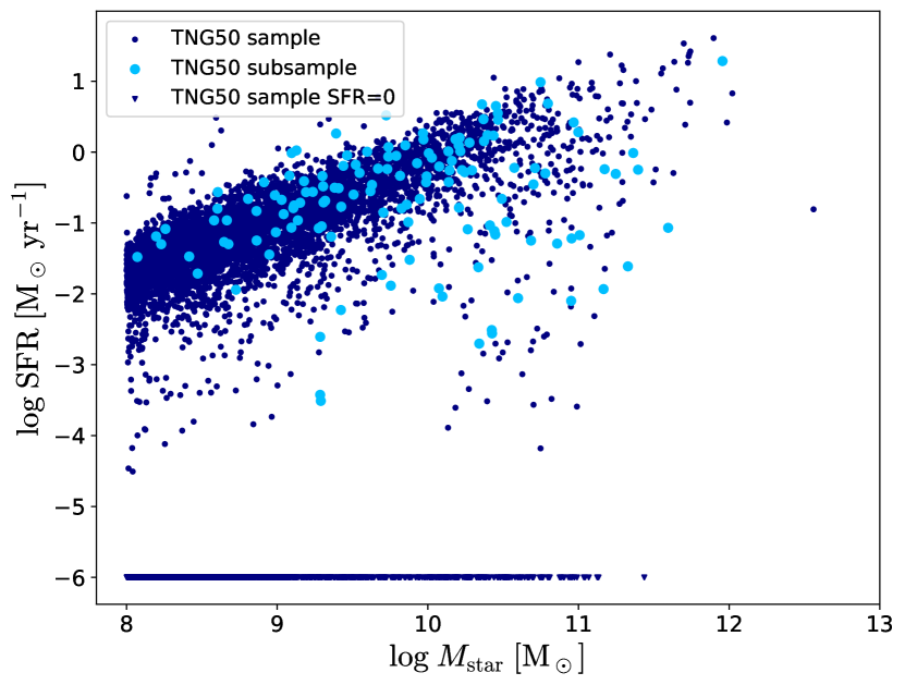
Figure 1: The main sequence of the $z=0$ TNG50 sample used in this study (navy blue). The triangles with SFR of $10^{-6}\mathrm{M_{\odot}/yr}$ are those with unresolvable low levels of SFR. The TNG50 subsample used for the RT calibration against the DustPedia observed galaxies is shown in cyan.

2.2 The RT procedure

The RT post-processing of the TNG50 galaxies is based on the 3D Monte Carlo RT code skirt (Baes et al., 2011; Camps & Baes, 2015, 2020) (Version 9). The code treats the relevant processes of dust extinction, emission, scattering and self-absorption (Camps & Baes, 2015). skirt is fully parallelised (Verstocken et al., 2017) and it uses a suite of optimisation techniques to enhance efficiency (Baes et al., 2011; Baes et al., 2016). It is equipped with an extensive library of SED models, dust models and geometry models (Baes & Camps, 2015) and advanced spatial grids (Saftly et al., 2013; Saftly et al., 2014; Camps et al., 2013). In the past few years, skirt has been extensively used to generate synthetic observations for hydrodynamically simulated galaxies, including synthetic fluxes and SEDs (e.g., Camps et al., 2016; Trayford et al., 2017; Camps et al., 2018; Vogelsberger et al., 2020b), images (e.g., Saftly et al., 2015; Rodriguez-Gomez et al., 2019; Camps et al., 2022; Popping et al., 2022), and polarisation maps (Vandenbroucke et al., 2021).

2.2.1 Galaxy partitioning

The strategy applied here largely follows the previous work on the EAGLE (Camps et al., 2016; Camps et al., 2018; Trayford et al., 2017) and Auriga (Kapoor et al., 2021) simulations, albeit with a number of minor adjustments. For every TNG50 galaxy, we analyse three sources of light: evolved stars, the star-forming (SF) regions, and the diffuse dust.

Evolved stellar populations:

Information on the star particles is obtained directly from the simulation. To each star particle that is older than 10 Myr, we assign an SED from the Bruzual & Charlot (2003) family, based on the particle birth mass, metallicity, and age. The Chabrier (2003) IMF is assumed. For the smoothing length needed for the RT, we use the radius of the sphere surrounding 32 stellar particles centred on each particle. Test results corresponding to different values for the smoothing length are described in Appendix B. We argue that the adaptive smoothing length we adopt gives the most realistic results (Rodriguez-Gomez et al., 2019; Schulz et al., 2020), however, there is no single optimal value.

Star-forming regions:

The modelling of the star-forming regions includes the use of the mappings-iii SED template family (Groves et al., 2008), applied on the young star particles ($t$<10 Myr). The templates are typically used for this purpose (e.g. Camps & Baes, 2015; Trayford et al., 2015; Camps et al., 2018; Schulz et al., 2020; Kapoor et al., 2021) and they contain five free parameters: interstellar medium (ISM) pressure, compactness, SFR, photodissociation region (PDR) covering fraction, and metallicity.

• For the ISM pressure, we assume the value of $P/k=10^{5}\;\mathrm{K~{}cm^{-3}}$, where $k$ is the Boltzmann constant. This is an average value in the mappings-iii library (Groves et al., 2008), and a representative value given the relevant densities in the ISM in the TNG50 simulation galaxies and the effective ISM temperature (Springel & Hernquist, 2003). The specific choice of the ISM pressure value hardly affects the broadband fluxes (see Groves et al., 2008, their Fig. 4).

• The compactness parameter ($\cal C$) mostly regulates the FIR part of the spectrum, with higher values corresponding to the shift of the IR peak towards shorter wavelengths, or equivalently, towards higher dust temperatures. Similarly as we did for the pressure, we assume the typical value $\log{\cal C}=5$. However, we do not use the same value for all SF regions, but we sample from the Gaussian distribution with the mean 5 and $\sigma=0.4$ (Kapoor et al., 2021). This results in a more realistic blend of SEDs with different dust temperatures, similar to observed or simulated star forming regions (Utomo et al., 2019; Kannan et al., 2020).

• The SFR is calculated from the birth mass of the particle over 10 Myr, since the SED templates are assuming the constant SFR over 10 Myr.

• The PDR covering fraction ($f_{\mathrm{PDR}}$) describes to what extent the Hii regions are coated with the PDRs. As we possess the information on the particle age ($t$), and since it is expected that the PDRs will clear eventually, we adopt a parameter $\tau$ such that

  $$f_{\mathrm{PDR}}=e^{-t/\tau}$$ (1)

  (Groves et al., 2008, and references therein). If $\tau=0$ the SF region is completely transparent, while if $\tau=\infty$, the Hii region is completely covered with the PDR. Since the particle age is a discrete value, we perturb it slightly to introduce some diversity for the SF regions with the same age. This can affect the median galaxy $f_{\mathrm{PDR}}$ up to 0.05. We use $\tau$ as a free parameter.

• The metallicity is obtained from the simulation.

The mappings-iii templates use Starburst99 family of SEDs for single stellar populations (SSP) (Leitherer et al., 1999) and the Kroupa (2001) IMF, while for the older stellar populations, we use the Bruzual & Charlot (2003) SSP templates and the Chabrier (2003) IMF. While we could use this SSP library (and therefore also the Kroupa (2001) IMF) for the evolved stars as well, we opted not to, as this would produce a significant inconsistency with the IMF from the simulations, and later with the SED fitting. To investigate the actual difference between the two SSP libraries, we ran additional skirt simulations where we adopt only the Starburst99 templates for all stellar particles (young and evolved). The results of the test are shown in Fig. 16d. The median magnitude deviation for the 136 TNG50 galaxies has a maximum of 0.23 mag. This in turn would affect optical luminosities up to 0.1 dex.

Diffuse dust

The diffuse dust component is derived from the gas simulated by TNG50. To select gas cells eligible to contain dust, we apply the boundary from Torrey et al. (2012); Torrey et al. (2019) that separates the hot circumgalactic medium from the cooler gas,

$$\log\left(\frac{T_{\text{gas}}}{\text{K}}\right)=6+0.25\log\left(\frac{\rho_{\text{gas}}}{10^{10}~{}h^{2}~{}{\text{kpc}}^{-3}}\right),$$ (2)

where $T_{\text{gas}}$ and $\rho_{\text{gas}}$ are temperature and mass density of the gas, respectively. In the simulation, the cool gas experiences two density regimes, below and above a number density threshold of $0.13~{}{\text{cm}}^{-3}$. Gas with a density above this threshold is considered star-forming. We assume that dust can survive in these cool diffuse regions, and in the dense star-forming domains below the threshold line (2).

For each of these eligible gas cells the dust density $\rho_{\text{dust}}$ is calculated from

$$\rho_{\text{dust}}=f_{\text{dust}}\,Z_{\text{gas}}\,\rho_{\text{gas}},$$ (3)

where $Z_{\text{gas}}$ is the gas metallicity. The parameter $f_{\text{dust}}$ represents the amount of metallic gas confined in dust grains and this is the second free parameter in our procedure. As indicated in the next section, we keep $f_{\text{dust}}$ constant as it is difficult to constrain this parameter from observational studies. The assumed dust model is the THEMIS model for the diffuse ISM (Jones et al., 2017), with 15 grain size bins (Kapoor et al., 2021). In a recent study, Camps et al. (2022) analysed differences between the THEMIS and the commonly used Zubko et al. (2004) dust model in the context of the post-processing of the cosmological galaxy simulations. They state in their Appendix A, that since the THEMIS model is generally more emissive and that its grain population shows up to 25 per cent more extinction than Zubko et al. (2004), the agreement with the observations is wavelength dependant. We decided to use the THEMIS model as it is physically motivated (it is based on the laboratory data) and it reproduces observed properties of the Galactic dust (Jones et al., 2017).

Previous studies applied the same recipe to derive the diffuse dust mass, all including the star-forming gas, however, with a different temperature limit for the diffuse gas. For example Camps et al. (2016); Camps et al. (2018), Trayford et al. (2017), and Vogelsberger et al. (2020b) included only non star-forming gas with $T_{\text{gas}}<8000~{}{\text{K}}$, Schulz et al. (2020) and Popping et al. (2022) applied $T_{\text{gas}}<75000~{}{\text{K}}$, Ma et al. (2019) adopted $T_{\text{gas}}<10^{6}~{}{\text{K}}$ while Rodriguez-Gomez et al. (2019) did not include diffuse gas at all. Recently, Hayward et al. (2021) employed the threshold line (2) to calculate submm fluxes for the TNG galaxies (without performing RT simulations), and Kapoor et al. (2021) applied it in post-processing of the Auriga simulations (Grand et al., 2017).

It is a challenging task to constrain this threshold as the processes involving dust production, destruction and transport are still poorly understood. However, we note that the change of the cut can considerably increase the number of dust cells, and potentially significantly affect the galaxy attenuation curve. This would in turn affect the galaxy SED as it would modify the star-dust geometry (e.g., Narayanan et al., 2018), even if the amount of dust does not change (by regulating $f_{\mathrm{dust}}$). We show this effect in Fig. 2, where the two curves represent the SED of the same galaxy, with the same dust mass but with the different dust mass distribution (shown in the inset), based on the applied cut. We employ two distinct $f_{\mathrm{dust}}$ to scale the dust mass, and the properties of the SF regions are the same. We can see that the SED corresponding to the model with a compact dust distribution (red line) is more attenuated at short wavelengths and has a higher far-infrared (FIR) output. In the other case, the same dust mass has a more diffuse distribution, causing more star light to escape. The dust masses from the cigale (see Sec. 2.3.4) fitting of these two SEDs, as expected, are not the same. The flux in FUV changes 0.15 dex, while around the peak of the IR emission ($\sim$200\text{\,}\mathrm{\SIUnitSymbolMicro m}$$) it differs 0.17 dex.

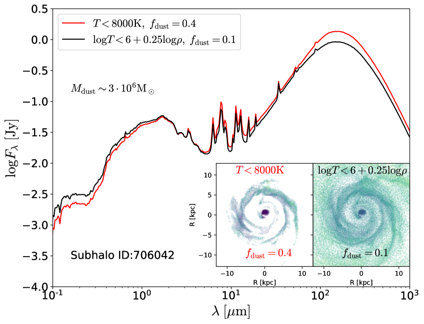
Figure 2: Two SEDs of the same TNG50 galaxy representing the effect of applying two different gas thresholds in the RT modeling. The dust mass is the same. The inset plots show the dust mass distribution for the two recipes.

Throughout this paper, we adopt the Torrey et al. (2012) recipe since it removes the hot and diffuse gas and, at the same time, incorporates all SF gas. Furthermore, Kapoor et al. (2021) found a slightly better agreement for the spatially resolved morphology parameters for the Auriga simulations with this dust recipe, compared to the more restrictive recipe from Camps et al. (2016).

2.2.2 Other RT parameters

In the TNG simulations, the gas hydrodynamics is modelled on a Voronoi mesh, which we also use to discretize the gas distribution as well as construct our medium (dust) system. However, for the dust discretization, we apply an octree grid to increase performance since the native Voronoi grid is not necessarily the most optimal grid for the RT simulations in terms of resolution (Camps et al., 2013; Kapoor et al., 2021). The octree grid implementation requires fixing several parameters. The maximum and minimum levels of grid refinement are important to ensure the balance between the resolution and the efficiency of RT procedure. The maximum level is set to 12, based on the aperture size of the biggest galaxy ($10R_{1/2,{\text{max}}}\approx 170$ kpc) and the gravitational softening length of the TNG50 simulation ($\epsilon=0.074$ kpc). For the minimum level, our test converged to 6. An additional and less strict condition is that the grid will refine as long as the maximum dust mass fraction is above $2\times 10^{-6}$. Finally, the selected number of photon packets to launch is $5\times 10^{7}$.

To verify the robustness of our procedure, as presented in Appendix B, we performed several tests including the derivations of the relative error, the variance of the variance and the Monte Carlo noise.

For each galaxy in our sample, we calculate the fluxes for three different angles: face-on, edge-on, and random. The first two are derived based on the galaxy stellar angular momentum and the third is given by the galaxy orientation in the simulation. Unless stated otherwise, for our analysis we exploit the random orientation.

Finally, skirt 9 allows for a high flexibility regarding the use of wavelength grids. Contrary to previous versions of the code, where a single fixed wavelength grid was used throughout the simulation, skirt 9 uses multiple independent wavelength grids, each specialized for a particular purpose (Camps & Baes, 2020). To calculate the dust emission spectrum in each spatial cell, we apply a nested grid with 100 logarithmically spaced bins, in the range from 0.2 to $2000\text{\,}\mathrm{\SIUnitSymbolMicro m}$, and 200 additional bins in the range from 3 to $25\text{\,}\mathrm{\SIUnitSymbolMicro m}$. In this way the emission region of small, stochastically heated dust particles is densely covered. The radiation field wavelength grid, used for storing photon packet contributions, contains 25 bins in range from 0.02 to $10\text{\,}\mathrm{\SIUnitSymbolMicro m}$. The total galaxy SED is collected in 450 bins between 0.02 and to $2000\text{\,}\mathrm{\SIUnitSymbolMicro m}$. These choices are motivated by a tradeoff between accuracy and performance (Camps & Baes, 2020).

2.3 The RT Calibration

The RT procedure introduced in the previous subsection has two global free parameters: the dust-to-metal fraction $f_{\text{dust}}$ and the PDR clearing timescale $\tau$. In this subsection we discuss how these two parameters are determined using a comparison to observations.

2.3.1 The DustPedia observational sample

To accurately calibrate the RT procedure of the simulated galaxies, it is necessary to have an appropriate observational sample. For this purpose, we decided to use the DustPedia sample (Davies et al., 2017) of 814 local galaxies with Herschel and WISE 3.4 $\mu m$ detections. The photometry of the sample is derived using the matching aperture method over a wide wavelength range, from the FUV to the submm (Clark et al., 2018). The DustPedia sample covers different environments (Davies et al., 2019) and contains sizeable samples of galaxies with different morphologies, stellar masses and dust masses (Bianchi et al., 2018; Nersesian et al., 2019; Mosenkov et al., 2019). Therefore, it is a representative sample of the local Universe with data covering the entire UV–submm wavelength range, optimal for our purpose.

2.3.2 Selection of a TNG50 calibration sample

The complete sample of the TNG50 galaxies we focus on in this study contains more than 14000 galaxies, as mentioned in Sec. 2.1. Since the calibration of the RT procedure of a sample this large would be immensely expensive, we carefully select a smaller calibration subsample. Since we will compare the simulations’ calibration sample with the DustPedia observational sample, it is important that these are similar. To achieve that, first we select TNG50 galaxies at redshift $z=0$, as the DustPedia sample comprises only local galaxies. We leave out galaxies with no SF (navy blue triangles in Fig. 1), as all DustPedia galaxies have non-zero SFR, reducing the TNG50 sample to 5787 galaxies. Fig. 3 compares the distributions of stellar mass and sSFR of the two samples, DustPedia and TNG50 in dark magenta and navy blue, respectively.

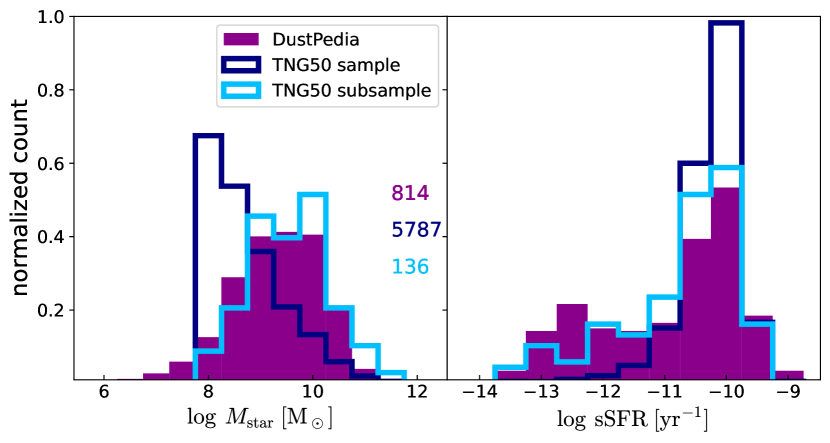
Figure 3: Distributions of stellar mass (left) and sSFR (right), for the DustPedia observed sample (dark magenta), the star-forming TNG50 simulated galaxies (navy blue) and the TNG50 subsample chosen to match the DustPedia sample and used for the RT calibration (light blue). Numbers represent the number of galaxies in each sample.

The stellar masses and sSFR values of DustPedia galaxies are derived using the cigale SED fitting tool (see Sec. 2.3.4), and for TNG50, we use the intrinsic data (inside $2R_{1/2}$). We then create a matched TNG50 subsample by random (rejection) sampling from the DustPedia galaxy stellar mass and sSFR distributions. For both distribution we identify 20 bins, and then we draw the appropriate number of galaxies in each bin. After the stellar mass selection, the initial TNG50 sample drops to 1730 galaxies, from which we try to match the sSFR distribution, so the final sample has 136 galaxies, shown in cyan. This new TNG50 sample, our calibration sample, is of manageable size and is more similar to the observed one, at least based on stellar mass and sSFR.

2.3.3 Aperture

The next step is to define the galaxy size or rather the aperture confining most of the galaxy light in different bands for each simulated galaxy. Different observational studies adopt different aperture definitions (e.g. Graham & Driver, 2005; Hill et al., 2011) and finding their analogues in the simulation realm is not straightforward. To tackle this problem, previous studies adopted various aperture definitions for the simulated galaxies: accounting for all particles (cells) gravitationally bound to the galaxy (Torrey et al., 2015), multiplying $R_{1/2}$ by a specific factor (Rodriguez-Gomez et al., 2019; Schulz et al., 2020; Popping et al., 2022), or applying a constant aperture for all galaxies (e.g. Camps et al., 2016; Camps et al., 2018; Trayford et al., 2017; Vogelsberger et al., 2020b). To achieve the most consistency, we decided to mimic the aperture size distribution of the DustPedia sample as a function of stellar mass. Fig. 4 represents this attempt. We see that the TNG50 3D apertures of $5\,R_{1/2}$ correspond well to the DustPedia apertures on the whole stellar mass dynamic range. How this aperture change affects the sample selection procedure is discussed in Appendix A. If not otherwise stated, the aperture of $5\,R_{1/2}$ is fiducial in this study, however, in Sec. 4.1.1 we will discuss the effects of aperture on the LFs.

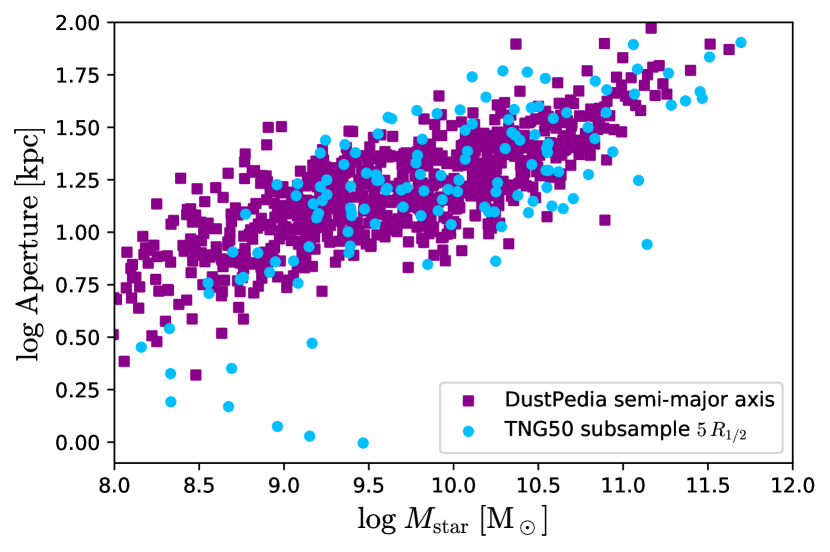
Figure 4: DustPedia apertures as a function of stellar mass (dark magenta), compared to the $5\,R_{1/2}$ apertures as a function of stellar mass for the TNG50 calibration sample (cyan). Here, the stellar masses for the DustPedia galaxies are inferred using cigale, those for the TNG50 galaxies are measured by summing the masses of the individual stellar particles.

2.3.4 SED fitting with cigale

Although each DustPedia galaxy on average contains reliable fluxes in 20 broadband filters, we perform an SED fitting procedure to improve the SED coverage and infer physical properties. Furthermore, to provide the most consistent comparison of the observational and the mock samples, we perform the same SED fitting procedure on the TNG50 calibration sample. We also use the same set of bands as those used for the fitting of the DustPedia galaxies. We exploit the SED fitting tool cigale (Boquien et al., 2019), which relies on the Bayesian inference technique and which employs a range of highly configurable models. For our purpose, we adopted a set of parameters that were fine-tuned for the DustPedia sample and are described in detail in Nersesian et al. (2019). In summary, we assume a truncated delayed SF history (Ciesla et al., 2016), the Bruzual & Charlot (2003) SSP libraries, the THEMIS model for the dust emission (Jones et al., 2017), and a modified Calzetti et al. (2000) curve (Boquien et al., 2019) for the dust attenuation. Compared to Nersesian et al. (2019), the only parameter we updated in this study is the IMF, where we selected Chabrier (2003) instead of Salpeter (1955), consistent with the cosmological and RT simulations.

The cigale fitted SEDs differ from the ones derived from skirt always less than 0.1 dex and mostly less than 0.05 dex. Therefore, we are confident that the fitted and the input fluxes can be used interchangeably. Furthermore, in Appendix C.1 we calculate the difference between the intrinsic galaxy properties and those derived from cigale. The median deviation is less than 0.14 dex. Therefore, for the calibration we will use the physical properties and fluxes derived from the SED fitting for both observational and simulated ’calibration’ samples. In this manner, both samples have the same wavelength coverage and are treated adopting the same models, alleviating the potential biases during the calibration.

2.3.5 Determination of the RT free parameters

The essential and final step before we run the RT procedure on the whole TNG50 sample is to specify the remaining free parameters of the procedure: $\tau$ and $f_{\mathrm{dust}}$.

The first parameter ($\tau$) controls the level of exposure of hii regions, and ranges from 0 to $\infty$. The higher this value, the more the Hii region is covered by the PDR layer. By construction, this parameter also affects the diffuse dust, as the amount of radiation that does not illuminate the dust in SF regions (if $\tau$ is small) will propagate into the ISM to heat the diffuse dust. Contrary, if $\tau$ is large, the energy will not leave the SF region, and the heating of the diffuse dust will be reserved mostly for the older stars. We chose to vary the parameter $\tau$ instead of $f_{\text{PDR}}$ (defined in formula 1), so we can mimic the spread in the covering factor relating to the clearing of SF regions as time progresses. Fig. 5 shows how the median $f_{\mathrm{PDR}}$ of our TNG50 subsample changes with $\tau$. For very low $\tau$ all galaxies have almost all SF regions completely open. At values as high as $\tau=11$ Myr, most of the SF regions are $60\%$ covered.

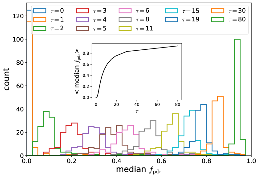
Figure 5: Distributions of the median $f_{\mathrm{PDR}}$ for different values of $\tau\mathrm{[Myr]}$, for the 136 TNG50 galaxies in the calibration subsample. The inset shows that with the increase of $\tau$, distributions of the median $f_{\mathrm{PDR}}$ peak at higher values.

The dust-to-metal fraction ($f_{\mathrm{dust}}$) directly controls the diffuse dust mass, as explained in Sec. 2.2.1. A growing body of literature has investigated this parameter for various galaxies and at different redshifts. While some studies suggest a trend with different galaxy properties like metallicity, stellar mass, or redshift (De Cia et al., 2013; Zafar & Watson, 2013; Rémy-Ruyer et al., 2014; De Vis et al., 2019; Péroux & Howk, 2020), these relations all have a relatively wide spread. De Vis et al. (2019) reported that for a DustPedia sub-sample of 364 galaxies the median $f_{\mathrm{dust}}$ is 0.2 with a range [0.03-0.64]. However, the physical properties in the observational studies are derived in a different way than in the simulations: it is therefore challenging to constrain this parameter directly from observations (although see Popping et al., 2022). Additionally, our current study focuses on galaxies with stellar masses above $10^{8}~{}{\text{M}}_{\odot}$ and at low redshift, thus the potential evolution of $f_{\text{dust}}$ would be less supported than at higher redshift. Accordingly, we opt not to vary $f_{\text{dust}}$ for different galaxies, and to treat it as a global free parameter. We explored a recipe variation where we add random noise to $f_{\text{dust}}$ for different dust cells, while keeping the integral value constant. The results are presented in Appendix B and the deviations are negligible.

In their work on the EAGLE simulations, Camps et al. (2016) calibrated the RT procedure by comparing mock and observational galaxy scaling relations. They used three scaling relations that incorporated several bands: three SPIRE, three SDSS and the GALEX NUV band. In a later study, Trčka et al. (2020) speculate that the exclusion of the FUV and MIR bands during the calibration can explain the high UV output seen for the EAGLE simulations (Baes et al., 2019), as the emission from the SF regions was not constrained sufficiently. Therefore, we decided to extend the SED coverage used in the calibration by including FUV, WISE 22, MIPS 70 and PACS 160 bands. The set of scaling relations includes those from Camps et al. (2016) (with $L_{$3.4\text{\,}\mathrm{\SIUnitSymbolMicro m}$}$ and $L_{$250\text{\,}\mathrm{\SIUnitSymbolMicro m}$}$ instead of stellar and dust mass, respectively), one with the alternative sSFR proxy ($L_{FUV}/L_{$3.4\text{\,}\mathrm{\SIUnitSymbolMicro m}$}$ instead of $\mathrm{NUV}-r$) and four showing extensive relations. With this set, we incorporate the data from 10 different bands, from FUV to submm. As stated previously, all quantities are derived with the cigale tool.

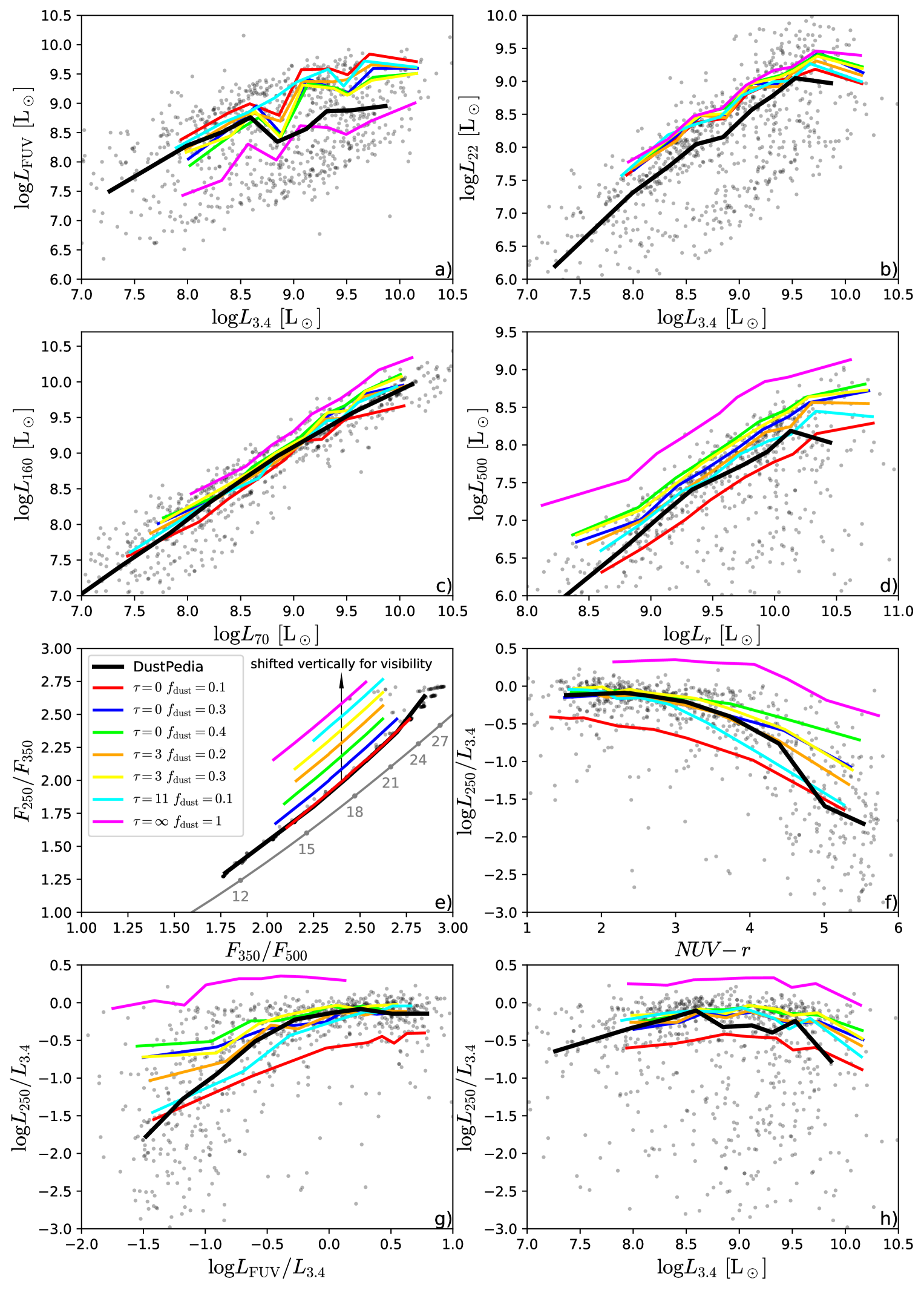
Figure 6: Eight $z=0$ galaxy scaling relations derived from fitting galaxy SEDs with CIGALE for both observed (DustPedia, black solid thick curves) and simulated (TNG50, coloured solid thin curves) galaxies. For the latter, curves represent the running medians of the different SKIRT RT recipes. The grey line in plot e) represents a modified blackbody (MBB) curve assuming the THEMIS dust model. The grey numbers correspond to the dust temperature in K. If not shifted, the lines in plot e) would overlap. The data points correspond to the DustPedia galaxies.

The results of our calibration exercise are shown in Fig. 6. The DustPedia data are shown in black. For the visual comparison of different recipes, we show the running median lines. Moreover, for a more quantitative valuation of the recipes, we performed the two-dimensional Kolmogorov-Smirnov test (KS test, Kolmogorov, 1933; Smirnov, 1948; Peacock, 1983; Fasano & Franceschini, 1987) on each scaling relation. This test provides us with two statistics: $p$-value and $D$-distance between the distributions. For each recipe, we derive the median of the eight $D$-values and compare these to find the recipe with the smallest distance from the DustPedia sample. First, we ran a set of RT simulations with extreme parameter values to explore the range of the parameter space. These are shown in Fig. 6 as red and magenta median lines. Comparing to the DustPedia in black, the two generally show poor agreement: the KS test gives $D=0.32$ and $D=0.48$ for the prescription with $\tau=0$ and $f_{\text{dust}}=0.1$, and $\tau=\infty$ and $f_{\text{dust}}=1$, respectively, i.e., with minimum and maximum dust in both compact and diffuse regimes. These differences emphasise the importance of dust in the galaxy modelling.

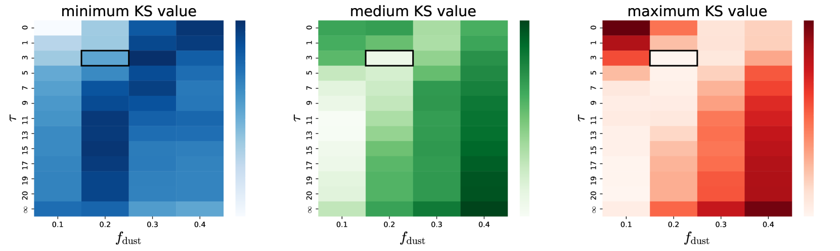
Figure 7: Minimum (left), median (centre), and maximum (right) KS statistic $D$ of the eight relations shown in Fig. 6, for the different values of $f_{\text{dust}}$ (x-axis) and $\tau$ (y-axis). Lower values that indicate smaller distance between the distributions are mostly located on a diagonal strip. For our fiducial RT modeling we adopt $f_{\text{dust}}=0.2$ (x-axis) and $\tau=3$ (y-axis), indicated with black rectangles.

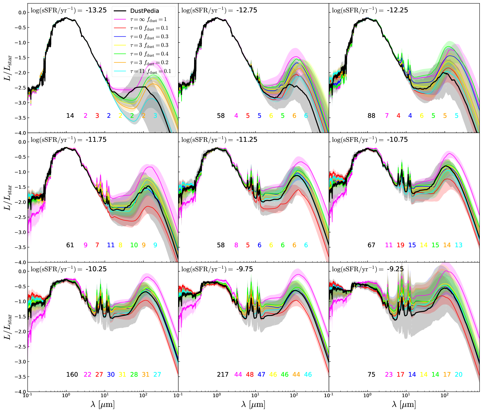
Figure 8: Median SEDs for the DustPedia observed galaxies (black) and for the TNG50 subsample for a number of RT-modeling choices, in bins of $\log$ sSFR at z=0. The shaded regions represent 16$\%$ - 84$\%$. The numbers of galaxies in each bin and each recipe are also shown, at the bottom.

Beside these two extreme recipes, we explored a full range of other, more physical options. The results of the KS tests for some of these are shown in Fig. 7. These panels show that there are several favourable parameter combinations, mostly towards low $f_{\text{dust}}$ and high $\tau$ values. Some of them are shown as well in Fig. 6.

While the results of the KS test show that there is a degeneracy among the two parameters (increasing $\tau$ and decreasing $f_{\text{dust}}$, and the opposite give a constant $D$ value), such degeneracy can be broken if we analyse the median lines of the individual scaling relations.

• Panel 6h represents the relation between the luminosity at $3.4\text{\,}\mathrm{\SIUnitSymbolMicro m}$ and $L_{250}/L_{3.4}$ (stellar and specific dust mass proxy, respectively). While the recipes in colour show similar results over the wide dynamic range, for the most massive systems the dust mass trends depend mostly on $f_{\text{dust}}$. This is expected since most massive systems have little or no SF regions.

• On the other hand, $L_{3.4}$, which traces emission from evolved stars, remains fairly constant with the recipe change. This is foreseen since we are not modifying this source, and the dust extinction is weak. However, hot dust also emits at these wavelengths. This can be seen in the same plot as the low $L_{3.4}$ limits of the medians change depending on the amount of diffuse dust (depending on $f_{\text{dust}}$) and the capability of the young stars to heat the dust (depending on $\tau$). In contrast, for the massive (and passive, as they have lower $L_{250}/L_{3.4}$) end this effect would be insignificant (Norris et al., 2014).

• Another relation that can be used to untangle the effects of the two parameters is in panel 6g, or equivalently panel 6f. On the x-axis they have a similar tracer for the sSFR, while on the y-axis they show a proxy for the specific dust mass ($M_{\text{dust}}/M_{\star}$). For galaxies with low sSFR, the parameter $\tau$ becomes irrelevant (recipe with a different $\tau$ and the same $f_{\mathrm{dust}}$ converge). If we follow the median lines in the direction of increasing UV for a fixed stellar mass, the results become more sensitive to the content of the SF regions.

• The plot in panel 6e shows the FIR colours. This relation is constrained by the SED fitting, however, the same relation with the ‘raw’ pre-cigale data is also fairly tight, particularly for the simulated galaxies, as there are no observational effects (see also Camps et al., 2016; Camps et al., 2018; Kapoor et al., 2021). As the medians overlap, we shift them by 0.1 dex to increase visibility. This relation gives us information about the galaxy dust temperature, as these flux ratios describe the slope of the IR emission. This color-color plot can be used to check whether the TNG50 galaxies have physical dust temperatures, since the limited resolution can produce an unrealistic stellar/dust configuration (Camps et al., 2018). All galaxies from the TNG50 calibration sample are sufficiently resolved and they populate the same temperature range as the DustPedia galaxies, however, mainly with intermediate values. As we see from the positions of the median lines, it is difficult to clearly unravel the individual contribution of the parameters, especially since the relation is also sensitive to the geometry of its components.

• The relation in panel 6c between luminosities in bands from both sides of the IR peak emission shows high agreement regardless of the recipe, while panel 6d shows that, on a contrary, in some cases the discrepancy can be up to an order of magnitude. Furthermore, in this plot (similarly also in panel 6h) we can see that at the high stellar mass end (high $L_{r}$) the dust output, while decreasing, is still too high. These two panels generally show poorer agreement irrespective of the recipe.

• Finally, in panel 6a, the break in the median line of the DustPedia galaxies demonstrates the bimodality in the relation, while this trend is less obvious for the simulated sample, and for the high stellar mass galaxies, the FUV emission is too high.

It is clearly challenging to select one ideal recipe: there is no single recipe that scores best in each of the individual panels of Fig. 6. This is also evident from Fig. 8, which shows the effect of the different recipes on the global galaxy SEDs. The individual panels contain the median SEDs of a number of recipes for different sSFR bins. The SEDs are normalised by the total stellar luminosity derived from cigale. We can see that, for low sSFR galaxies, dust emission greatly varies between the recipes, with minimal change in the UV. These galaxies have few or no young stars, therefore intrinsically very little UV to be attenuated. For higher sSFR values the UV and FIR domains are fitted remarkably well employing a number of recipes, while the MIR range shows increasingly poorer agreement. This implies that for every parameter configuration the TNG50 galaxies with high sSFR will have an excess of very hot dust. Reviewing the different galaxy populations in Fig. 8, we see that in distinct sSFR bins and wavelength regimes, different recipes show better agreement. Even the nonphysical recipes with $f_{\mathrm{dust}}=0.1$ and $\tau=0$, and with $f_{\mathrm{dust}}=3$ and $\tau=\infty$, do not show the highest discrepancies for $\log(\mathrm{sSFRs}/\mathrm{yr})$ between $-13$ and $-12.25$. We do note, however, that most of the (physical) recipes presented in Figs. 6 and 8 are within the errors and spread of the DustPedia data along the whole wavelength range, meaning that our procedure is robust and that the final selection is merely fine-tuning.

Based on the deviations between the median SEDs in different sSFR bins and the KS scores, we conclude that, on average, the recipes with $f_{\text{dust}}>0.2$ are the least favourable, regardless of $\tau$ ($D>0.282$). Furthermore, the recipes with a fixed $f_{\text{dust}}$ and a high $\tau$ show similar results, as the differences between the total covering fractions are getting smaller (see equation 1 and Fig. 5).

The two parameter combinations that we finally consider are the one with $f_{\text{dust}}=0.1$ and $\tau=11$ Myr (fd1-t11, hereafter) with $D=0.243$, and the one with $f_{\text{dust}}=0.2$ and $\tau=3$ Myr (fd2-t3, hereafter) with $D=0.252$. The main differences between these two recipes are in the MIR and FIR for galaxies with low sSFR (orange and cyan lines in Fig. 6 and Fig. 8). For all sSFR bins, the fd2-t3 dust prescription has a higher MIR output. This is a consequence of, on average, mostly open Hii regions (see Fig. 5) from which the UV radiation is now heating more diffuse dust, compared to the fd1-t11 scheme. Both options produce comparable FIR output for moderate and high sSFRs. For the low sSFR galaxies, there is a lack of compact dust to increase the IR emission for high values of $\tau$, therefore the discrepancy between the two dust allocation recipes is higher. Nevertheless, for the whole calibration sample, the difference in the dust mass (from cigale) is on average $\approx 0.15$ dex. Since these two recipes similarly affect a galaxy SED, we decided to adopt fd2-t3 as the fiducial dust distribution, as this value of $f_{\text{dust}}$ is comparable with that of the DustPedia and other observational samples (De Vis et al., 2019; Zabel et al., 2021; Galliano et al., 2021). So, throughout this work, simulated galaxies are post-processed with skirt with $f_{\text{dust}}=0.2$ and $\tau=3$. In Sec. 4.1.3 we address the effect of different RT choices on the LFs.

One question that arises is whether our results would change if we had chosen another set of scaling relations for the calibration. To test this, we analysed the distribution of the KS scores if we only include relations used in Camps et al. (2016), and the results qualitatively do not change. Analysing a set of relations that all include one galaxy property on one axis, such as stellar mass ($L_{3.4}$) or dust mass ($L_{250}$), does not bring our results to convergence. This approach can be successfully applied to simulations of less diverse galaxy populations (Kapoor et al., 2021), however, for most properties, our sample spans three orders of magnitude, with a result that different recipes agree better for distinct galaxy populations (e.g., see Fig. 6a).

Finally, we note that, for a different definition of a dust tracer (see 2.2.1: Diffuse dust), an another set of parameters might be selected as the optimal set. For example, Kapoor et al. (2021) compared two definitions: the one based on the threshold from Torrey et al. (2012) (the fiducial in this study), and the one restricting dust only to star-forming gas cells. Compared to the former, the latter definition requires higher values of $f_{\text{dust}}$ for optimal results.

3 Results

3.1 UV to submm fluxes

We apply our fiducial RT modeling to the whole TNG50 sample with $M_{\star}>10^{8}~{}{\text{M}}_{\odot}$ (see Fig. 1). Including galaxies without dust and the small sample used for calibration, the final sample contains 7375 galaxies at $z=0$ and 7302 galaxies at $z=0.1$. Furthermore, we apply the same RT procedure to TNG50-2, the TNG50 run with one step worse resolution (a factor of eight in particle mass, two in spatial resolution). To ensure a similar number of stellar particles per galaxy ($\sim$ 1000), for TNG50-2 we impose a stellar mass threshold of $\log M_{\mathrm{star}}/\mathrm{M_{\odot}}>8.6$. Therefore, for TNG50-2 we have 3559 galaxies at $z=0$ and 3497 galaxies at $z=0.1$. For the redshift $z=0,$ the fluxes are calculated assuming the galaxies are at 20 Mpc from the detector, consistent with previous studies (Camps et al., 2016; Trayford et al., 2017).

To validate our procedure, in Appendix C.2 we investigate the differences between the true values of the galaxy stellar masses and SFRs and those calculated from the fluxes, based on recipes from the literature.

Finally, we publish the data for future science projects. Tables 1 and 2 summarise the available information. Broadband fluxes of the total galaxy emission are calculated in 53 bands, for two resolution options of the TNG50 simulation, two redshifts, four different apertures and three orientations. The same options are available for the galaxy SEDs.

Table 1: Structure of the published data. Resolution: different resolution runs of the TNG50 simulation. Redshift: galaxy redshift (if $z=0$, the flux is calculated at 20 Mpc). Aperture: 2D circular aperture used to extract SED. Orientation: angle at which the galaxy is observed. Component: the integrated flux at different wavelengths and in 53 broadbands. Every combination is provided.

Resolution	TNG50
	TNG50-2
Redshift	0
	0.1
Aperture	$5R_{1/2}$
	$2R_{1/2}$
	10 kpc
	30 kpc
Orientation	face-on
	edge-on
	random
Component	total
	total - broadbands

3.2 Galaxy luminosity functions at $z\leq 0.1$

The complete low-redshift TNG50 sample comprises 14677 galaxies, which allows us to inspect the LFs and compare them with the observed ones. We perform the study over a wide range of wavelengths, from the UV to the submm range. However, we omitted the MIR bands, since the available data from the literature is typically presented in a wider redshift range, which would produce an inconsistent comparison (Baes et al., 2020). Instead, we also investigate the total IR luminosity.

All TNG50 LFs are derived by splitting the population of galaxies in $\log L$ bins and dividing by the simulation co-moving volume, while the errors are derived following Poisson statistics. As we consider galaxies above a certain stellar mass threshold ($\log M_{\mathrm{star}}/M_{\odot}>8$ for TNG50 and $\log M_{\mathrm{star}}/M_{\odot}>8.6$ for TNG50-2), the low-luminosity bins are incomplete. To derive the minimum luminosity where these bins may be complete, in the narrow stellar mass mass bin at the low limit, we calculate the 90th percentile of the luminosity distribution. We select this value (calculated for each band) as a low cut for the galaxy LF.

Finally, to calculate the total IR luminosity, we implement the five-band formula for nearby galaxies from Galametz et al. (2013), i.e.

$$L_{\text{TIR}}=2.023\,L_{24}+0.523\,L_{70}\\ +0.39\,L_{100}+0.577\,L_{160}+0.721\,L_{250}.$$ (4)

When this formula was applied to the sample of galaxies from the EAGLE simulations (Schaye et al., 2015; Crain et al., 2015) and compared to the luminosities derived from cigale, the results showed excellent agreement (Baes et al., 2020).

3.2.1 Observational LFs

In this study, we compare the simulated TNG50 LFs with a number of observational LFs. In the UV regime, in two GALEX (Morrissey et al., 2007) bands, we compare to the data from the GALEX MIS survey (Budavári et al., 2005, $0.07<z<0.13$), and from the shallower AIS survey (Wyder et al., 2005, $z<0.1$). Additionally, we use LFs covering the entire UV to NIR range (Driver et al., 2012, $0.013<z<0.1$) from the GAMA survey (Driver et al., 2011; Liske et al., 2015). Focusing solely on the optical, Loveday et al. (2012) calculated LFs from the full GAMA survey, but with the original SDSS (York et al., 2000) magnitudes. Combining SDSS, UKIDSS LAS (Lawrence et al., 2007) and the MGC redshift survey (Liske et al., 2003), Hill et al. (2010) derived LFs for $0.0033<z<0.1$. In the IR domain, at $250\text{\,}\mathrm{\SIUnitSymbolMicro m}$ we have the LF (Dunne et al., 2011, $z<0.1$) from the H-ATLAS survey (Eales et al., 2010; Rigby et al., 2011), with redshifts from the GAMA survey. At $350\text{\,}\mathrm{\SIUnitSymbolMicro m}$, we compare our results with the LF from (Negrello et al., 2013, $z\lll 0.1$) based on the Planck ERCSC (Planck Collaboration et al., 2011) data. For all SPIRE bands and the total IR, we use the LFs from (Marchetti et al., 2016, $0.02<z<0.1$) based on the HerMES survey (Oliver et al., 2012), combined with the Spitzer Data Fusion database (Vaccari, 2015).

All data from the literature are converted to AB magnitudes and to $h=0.6774$, to match the simulated data.

3.2.2 LFs of the TNG50 simulations

In this section, we assume the fiducial set of parameters: $5\,R_{1/2}$ apertures, random galaxy orientations, the fd2-t3 RT fiducial procedure recipe, the TNG50 simulation at available resolution. Namely, we integrate the light coming from (approximately) cylindrical volumes around each galaxy with radius of $5\,R_{1/2}$ in the plane of the sky and with a depth of $10\,R_{1/2}$. The results are shown in Fig. 9.

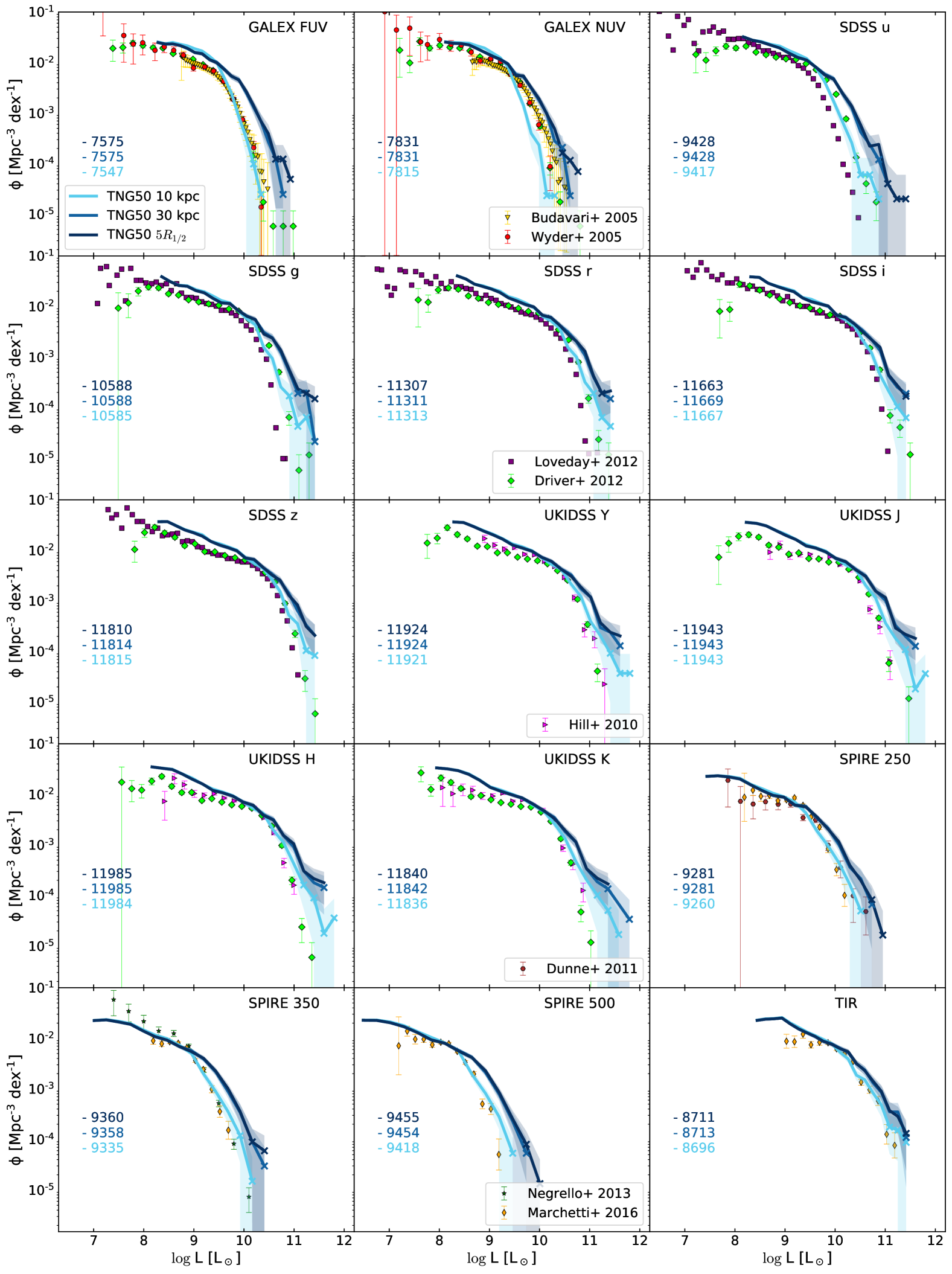
Figure 9: LFs in in 14 bands and the total IR LF, at $z\leq 0.1$. The navy blue lines correspond to TNG50, post processed with SKIRT according to the RT procedure described and devised in the previous Sections, with light summed up from an aperture of $5\,R_{1/2}$ for each galaxy. The other blue lines show results for different apertures. The ’x’ marker depicts luminosity bins with fewer than 10 objects. Shaded region shows the Poisson error. The number on the left represents the total number of the TNG50 galaxies. We give the LFs from the simulated galaxies only above the completeness limit imposed by the selection: stellar mass $>10^{8}\;\mathrm{M_{\odot}}$. The coloured symbols represent observational data.

By inspecting the fiducial TNG50+RT model (in navy blue) over a range of wavelengths, we immediately notice that the TNG50 LFs tend to overpredict the observational ones. At the faint end, TNG50 best agrees with observations in the near UV, in the optical u band and across the IR wavelengths. The largest disagreements, at the faint end, are in the central optical wavelength. One case where the simulated LFs underpredict observations is the faint end of the SPIRE $350\text{\,}\mathrm{\SIUnitSymbolMicro m}$ LF measured by Negrello et al. (2013): however, as stated in Sec. 3.2.1 this LF is inferred in the very local Universe where the contamination and inhomogeneities can be large (Marchetti et al., 2016), whereas our sample more closely connects to the deeper observations from Marchetti et al. (2016).

We quantify the level of (dis)agreement between TNG50 and observed LFs in Fig. 10. This figure shows the median discrepancy between observations in three luminosity regimes: $\pm$ 0.2 dex around the knee of the LFs in the brighter and fainter ends (the position of the knee, acquired from Driver et al., 2012; Marchetti et al., 2016, is based on the characteristic luminosity of the Schechter function fit). Here the light from each galaxy is obtained by summing up all the contribution from within $5\,R_{1/2}$. Comparing the whole LFs, the FUV band shows the poorest agreement, mostly because of the disagreement at the bright end; the SPIRE 250 band instead shows the best agreement. In the UV and FIR domains, the TNG50 faint end has better agreement than the bright end, while in the optical and NIR only the knee of the LFs is reproduced to within 0.04 dex. The discrepancies do not seem to correlate with the wavelength, or only weakly. The shape of all LFs at the faint end closely follows that of the observations, where the upturn in some observational LFs at low luminosities (Hill et al., 2010; Loveday et al., 2012; Driver et al., 2012) is visible in the simulations a s well. We will return to explore this feature in Sec. 4.2, where we analyse different galaxy populations.

Since the TNG50+RT fiducial model shows discrepancies as high as 0.8 dex, in the rest of the paper, we explore different drivers of the galaxy LF shape and normalisation.

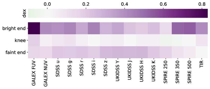
Figure 10: Median difference between the LFs of the TNG50 galaxies (with $5\,R_{1/2}$ apertures) and the observed LFs, at different wavelengths and at three luminosity regimes: $\pm$ 0.2 dex around the knee of the LFs and the brighter and fainter ends. The differences are in dex.

4 Discussion

4.1 Discrepancy between the observed and TNG50 LFs

In order to disentangle the effects of different assumptions and settings of our approach, we individually investigate how aperture, orientation, RT recipe and simulation resolution affect the LFs. For the parameters that are not being discussed, we assume the fiducial values. For brevity reasons, we discuss only the most relevant options, however all of them are presented at http://luminosity-functions.herokuapp.com/.

4.1.1 Aperture effect

We have measured the TNG50 LFs corresponding to four distinct circular aperture choices in the plane of the sky: $5\,R_{1/2}$ (fiducial), $2\,R_{1/2}$, 30 kpc, and 10 kpc. The dust and stellar distributions are calculated inside $5\,R_{1/2}$ for all apertures in 3D. This means that, along the line of sight, we always collect light from a depth of $10\,R_{1/2}$, while the field of view is limited by the specific 2D aperture size (with an effective maximum being $10\,R_{1/2}$ as there are no sources beyond that point). Restricting the field of view without the limit on the line of sight, we mimic the observational apertures. The results in different bands are presented in Fig. 9, in lighter colours compared to the fiducial model.

Comparing the aperture of 30 kpc to the fiducial one, as expected, the difference can be seen only at the bright end of the galaxy LF, which is now lower than when applying the fiducial aperture. A similar effect is observed for the $2R_{1/2}$ and the smallest 10 kpc aperture. The discrepancy between the apertures is less pronounced moving towards the NIR, because the emission from the older stellar population (that dominates the central galaxy region Casasola et al., 2017), has a higher contribution at these wavelengths.

Several observational studies demonstrated that the bright end of the LF heavily depends on the aperture adopted in the magnitude calculation (Hill et al., 2011; Bernardi et al., 2013). This effect can be seen analysing the observational results from Loveday et al. (2012) and Driver et al. (2012) in the optical, where former applied Petrosian (Petrosian, 1976) and latter Kron (Kron, 1980) magnitudes on the same data set. While there is an offset between the two magnitude systems, they both can greatly underestimate galaxy fluxes (Graham & Driver, 2005). Additionally, in the UV domain, the observational data is derived inside the Kron aperture, while in the FIR the apertures are difficult to handle due to the poor resolution and high confusion noise (Nguyen et al., 2010). In Appendix E we test how our different aperture definitions correlate with the Petrosian aperture. The $5R_{1/2}$ aperture shows a high correlation, while for massive galaxies 30 kpc can be a good approximation. With the aperture of 10 kpc is expected to be too small to collect the the same amount of light as the Petrosian aperture.

We conclude that, while (only) the bright end of the galaxy LF is sensitive to the aperture choice, applying another relevant aperture definition (30 kpc), does not improve the results.

4.1.2 Orientation effect

Our data release contains, for every galaxy, fluxes for three galaxy orientations: edge-on, face-on, and random (given by the simulation). This allows us to also consider edge-on and face-on LFs. The random view is useful for the general comparison with observational surveys, while the analysis of specific orientations can aid in defining potential biases in observational studies (Lovell et al., 2021; Yuan et al., 2021).

The variability of the LFs with the galaxy orientation depends on the wavelength. Moving from UV towards IR, the effect declines because the stellar emission fades, and the dust attenuation is low at longer wavelengths. The top row of Fig. 11 shows the LFs in a selection of bands across the SED. In the UV, where the effect is most pronounced, we can see the impact of dust on the young stellar emission, as there is a considerable drop in the number of UV luminous objects as the inclination angle increases. These galaxies are increasingly star-forming, dusty, and largely asymmetrical. The effect is the same for every galaxy aperture.

If our sample included high-redshift and/or ultraluminous infrared galaxies (ULIRGs; $10^{12}L_{\odot}<L_{\mathrm{IR}}<10^{13}L_{\odot}$), that are compact, extremely star-forming and with hot dust (Casey et al., 2014) it would be necessary to incorporate the dust self-absorption in our RT procedure (Camps et al., 2018; Ma et al., 2019). For these objects, if they are disk-like, the results would then vary with the inclination in a wider wavelength range (Lovell et al., 2021).

In conclusion, since our observational samples do not favour any particular orientation, the fiducial model with the random view is the most compatible for the comparison. Furthermore, the effect of the orientation change can be only seen at low wavelengths.

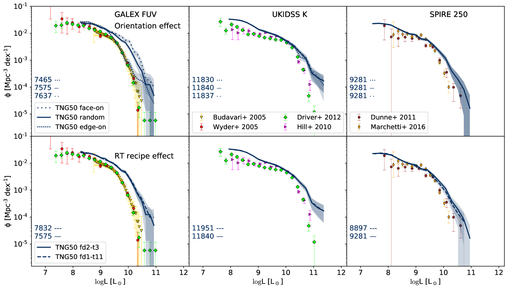
Figure 11: Similar as Fig. 9 but only for three bands and for the different galaxy orientations (RT recipes), top (bottom). The solid line represents the fiducial model, while (loosely) dotted denotes (face-on) edge-on view, and dashed the fd1-t11 RT recipe.

4.1.3 RT recipe effect

One possible explanation for the discrepancies between observations and simulations could be that our RT settings are ill-chosen. Repeating the RT procedure on the whole TNG50 sample with different choices for the RT post-processing recipe is a highly resource-intensive job. However, to understand to what extent the recipe affects the LFs, we decided to repeat the procedure and recalculate the LFs for the fd1-t11 recipe. As stated in Sec. 2.3, the fiducial fd2-t3 recipe and the fd1-t11 recipe differ in both the diffuse and compact dust: the former has larger amounts of diffuse dust, while the latter assumes more screened Hii regions.

The bottom panel of Fig. 11 shows that the choice of the RT recipe has a very modest effect on the LFs. The recipe with low $f_{\text{dust}}$ displays an emission excess across the UV and optical range, which demonstrates that, in our setting, the diffuse dust is driving the results. In the FUV the recipes agree with each other despite the difference in the $f_{\text{dust}}$ and $\tau$. In this band the emission predominantly comes from young stars, therefore the additional coating of the hii regions can compensate for the lack of diffuse dust. Consequently, the fd1-t11 recipe has slightly lower IR emission than the fiducial recipe. Overall, however, the change of RT recipe does not bring the simulated LFs more in agreement with the observational data. The same conclusions are derived if we compare the RT recipes assuming different aperture definitions.

4.1.4 Hydrodynamic simulation resolution effects

The TNG simulations are realised with and without baryons, at a number of resolutions and box sizes (for an overview, see Table 1 in Nelson et al., 2019b).

The TNG model was designed at a resolution similar to the one of the original Illustris simulation, i.e, at the resolution of the other flagship run of the IllustrisTNG project, TNG100 (Pillepich et al., 2018b; Nelson et al., 2018; Naiman et al., 2018; Marinacci et al., 2018; Springel et al., 2018). The TNG100 and TNG50-2 simulations adopt comparable resolutions. The other resolution simulations were run by assuming exactly the same physical model and subgrid parameter values (Pillepich et al., 2018a). This approach can manifest as quantitative changes in the simulations’ outcome for different adopted numerical resolutions, to different degrees depending on the galaxy properties under scrutiny (Pillepich et al., 2018a, b, 2019). To explore how the resolution of the cosmological hydrodynamical galaxy simulation influences our results, we have repeated our analysis for the TNG50-2 simulation, which has 8 (2) times worse mass (spatial) resolution than the flagship TNG50 run. For this, we have assumed and applied the same fiducial RT modeling (i.e. adopted the same calibrated RT parameters as for TNG50) and recalculated LFs starting from the data simulated by TNG50-2. As it has been shown that, within the TNG model, an improved resolution may result in somewhat larger galaxy masses and SFRs (Pillepich et al., 2018a, b, 2019; Donnari et al., 2019), we can expect to see a downshift in the LFs when moving from TNG50 to TNG50-2.

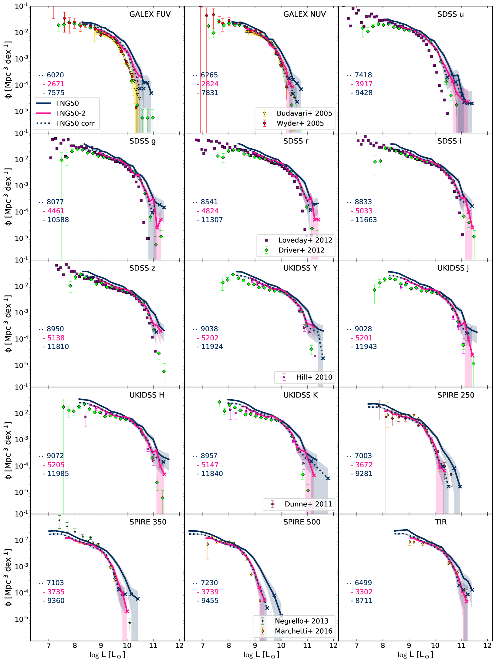
Figure 12: Same as Fig. 9 but comparing the results from TNG50 (navy blue) to a worse-resolution counterpart called TNG50-2 (pink), with 8 (2) times worse mass (spatial) numerical resolution, both post-processed with the same fiducial RT modeling. The navy blue dotted line represents a possible way to correct the TNG50 results to account for the effects of resolution. In all curves, light from each galaxy is taken from a $5\,R_{1/2}$ aperture. We give the LFs from the simulated galaxies only above the completeness limit imposed by the selection: stellar mass $>10^{8}\;\mathrm{M_{\odot}}$ ($10^{8.6}\;\mathrm{M_{\odot}}$) for TNG50 (TNG50-2).

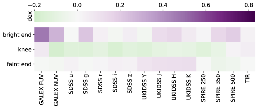
Figure 13: Same as Fig. 10 but for the TNG50-2. The colour bars are showing the same range as in Fig. 10.

The results are presented in Fig. 12. As expected, we see that TNG50-2 has lower LF values across the entire wavelength range. The agreement with the observed LFs is substantially improved, which we quantify in Fig. 13. This finding reveals that the two simulation runs behave in the same way in the observed space and across the whole wavelength range as noticed in the physical space. Therefore, we expect the same high level of agreement of the galaxy LF between TNG100 and observations, since the stellar masses of halos, and so also the stellar mass function, decrease with worse numerical resolution (as discussed e.g. in Pillepich et al. (2018a) Appendix A on the TNG model convergence, and Pillepich et al. (2018b) Appendix A on the TNG100/300 convergence).

From the comparison between TNG50 and TNG50-2, we can derive a resolution correction to be applied to TNG50. Following Pillepich et al. (2018b); Engler et al. (2021) and Vogelsberger et al. (2018, 2020b), and assuming that the resolution change does not affect the halo mass, we first subdivide the sample based on the halo mass. In each halo mass bin, we calculate the total luminosity in each band and redshift and for both simulation runs. The ratio of these values is the factor we use to scale the luminosity of each individual galaxy. The outcome of this exercise is shown as the navy blue dashed lines in Fig. 12, where we can see that the transition from TNG50 to TNG50-2 is excellent. An alternative way to improve the agreement with observations could have been obtained by adopting different choices in the TNG model (i.e. different subgrid parameter values) to account for the resolution change, prior to run the galaxy simulation, as done e.g. within the EAGLE project (Schaye et al., 2015; Crain et al., 2015) and demonstrated by Mitchell et al. (2021).

In the final overview of the simulated (both TNG50-rescaled and TNG50-2) and observed LFs, in most bands, we see an outstanding agreement. The minor excess at the very bright end is partially caused by the low statistics in the high luminosity bin. However, in the FUV band there is still an overabundance of luminous galaxies. This can still be attributed to the uncertainty about where i.e. with which aperture the observations are taken. At the same time, from Fig. 8 it can be seen that for the majority of recipes, the flux in the FUV band is typically much higher than the one in the NUV band, while the DustPedia sample has the opposite trend in most panels. In their previous work Baes et al. (2019) and Trčka et al. (2020) analysed the mock fluxes of the EAGLE simulations, derived in a similar manner as we employ here. These studies revealed that the UV part of the spectrum exhibits the highest discrepancy compared to the observations also in the case of EAGLE. This wavelength regime is difficult to constrain because, while the emission in the FUV emerges from the star-forming regions, they are still not resolved in the cosmological simulations. Therefore, the use of templates, like the mappings-iii templates we use here, is necessary. While we improved the method by introducing more realistic settings (time-dependent covering factor, variable compactness), we argue that there is a need for templates that can more successfully exploit the data from the simulations (Kapoor et al., in prep).

4.2 Contribution of different galaxy populations to the LF

We conclude the paper by analysing how distinct galaxy populations contribute to the LFs. We split our sample according to three different criteria: morphology, environment and star formation activity.

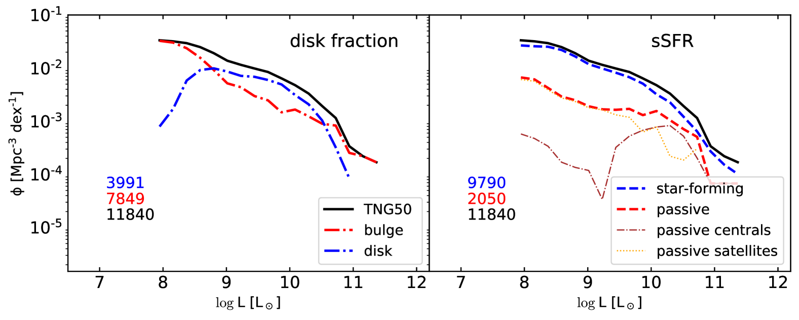
Figure 14: TNG50 LF in the UKIDSS K band at $z\leq 0.1$. The black line in both panels is the TNG50 LF inside $5\;R_{1/2}$ for the random orientation and fiducial RT recipe. Left: The red and blue dash-dotted lines correspond to the galaxies defined as a bulge and disk-dominated, respectively. Right: The red and blue dashed lines show how the sample splits according to the sSFR. The brown dot-dashed and orange dotted lines show the passive centrals and the passive satellites, respectively.

For the morphology, we apply a simple prescription to divide the sample into disk and bulge-dominated galaxies, by exploiting the stellar kinematical data (Genel et al., 2015). Based on their angular momentum, stars are assigned to either disk or bulge, and for a galaxy to be defined as disk-dominated, the mass fraction of disk stars should be over 0.35 (Hoffmann et al., 2020). We present the results in the left panel of Fig. 14, where we show the luminosity function in the UKIDSS K band. Since this band traces the emission of evolved stars and is insensitive to the SFR, this LF is a proxy for the stellar mass function. Bulge-dominated galaxies are prominent in both the bright and faint end of the LF, while disk galaxies dominate the LF at intermediate luminosities. Trayford et al. (2019) derived comparable results for the stellar mass function of the EAGLE simulations. Comparing to observations, Kelvin et al. (2014) calculated LFs for the GAMA survey and noticed a similar shift in the contribution of the different Hubble populations at the luminous end, although their sample contained mostly disk-like galaxies, contrary to our results. When we repeat the same exercise for the TNG50-2 simulation, we find that the number of disk galaxies decreases even more, as it is shown that the low resolution simulations have thicker disks (Pillepich et al., 2019). Analysing the visual morphologies of the TNG100 galaxies via machine learning techniques, Huertas-Company et al. (2019) derive similar results for the mass function, however their population split shows a lack of early type galaxies with high masses.

Moving to the star formation activity, we divide the sample into star-forming and passive galaxies, applying a cut in sSFR. Following Salim (2014), we identify galaxies as star-forming if ${\text{sSFR}}>10^{-10.8}$ yr^-1, and passive otherwise. We present the results in the right panel of Fig. 14. We see that the upturn, seen in the global LF at the faint end, is mainly driven by the shape of the LF for the passive galaxies. The existence and the origin of the upturn towards the faint end of LFs (and mass functions) have been heavily debated (e.g. Blanton et al., 2003; Hill et al., 2010; Loveday et al., 2012; Driver et al., 2012). Taylor et al. (2015) review different ways of subdividing a galaxy sample into blue and red galaxies, depending on the global colours. They argue that the reason a few studies show the presence of this upturn in the population of red galaxies is the contamination by the blue galaxies, due to inadequate sample splitting. We tested this hypothesis by changing our threshold in the sSFR and employing three different colour and stellar mass cuts (Bell et al., 2003; Baldry et al., 2004; Peng et al., 2010), but the shape of the passive LF remains the same. This result is not unexpected if we look at Fig. 1, where there is a clear bimodality in the stellar mass for the passive galaxies. To inspect this further, we split the passive sample into centrals and satellites, which revealed that most of the emission at the luminous end comes from the centrals, while the upturn is completely dominated by the passive satellites, in agreement with observations (Lan et al., 2016). The number of passive centrals, compared to the number of the passive satellites at low luminosities (stellar masses) is insignificant. This is a consequence of a generally small ratio of passive central galaxies at low masses (Geha et al., 2012), that is captured by the TNG50 simulations. As shown in, e.g. Donnari et al. (2021) and Joshi et al. (2021), going to worse resolutions (e.g. TNG50-2) will show an increased fraction of quenched low mass central galaxies.

Our findings demonstrate that different galaxy populations affect in a complex manner the LFs in simulations, in accordance with the observations.

5 Summary and Conclusions

In this study, we have produced mock fluxes over a wavelength range from FUV to sub-mm for low-redshift galaxies from TNG50, a state-of-the-art cosmological hydrodynamical simulation for galaxy formation. Using the skirt code we have calibrated the RT procedure on a small TNG50 subsample that corresponds to the observational DustPedia sample. The calibration constrains the amount of diffuse dust and the dust covering of the SF regions. The calibration was based on the comparison of various luminosity scaling relations and full galaxy SEDs (Figs. 6 and 8). Both the simulated subsample and the observed data from the DustPedia sample are processed using the cigale SED fitting code to ensure the comparison is consistent.

We applied the calibrated RT procedure to the whole TNG50 sample (and the worse-resolution TNG50-2 sample) and produced the observed fluxes and rest frame magnitudes in 53 broadbands for $z\leq 0.1$, for three orientations and four apertures. Full galaxy SEDs are also generated (Table 1). These data are publicly released (https://www.tng-project.org/trcka22) and we invite interested colleagues to use these data for their own science projects.

We have constructed and analysed the LFs for the TNG50 simulation over a range of broadband filters covering UV to submm wavelengths and compared them to different observational data. For our fiducial setting, we found agreement on the overall shape of the LFs and the normalization at the knee, however, the simulations mainly overestimate the observations (Fig. 9), with the best agreement for total IR at faint end ($\sim$ 0.004 dex) and with the strongest discrepancies in the FUV ($\sim$ 0.8 dex) at the bright end.

We varied several parameters in order to investigate their effect on the LFs, and we derived the following conclusions:

• Our results are sensitive to the aperture choice at the LF bright end across the wavelength range. However, the choice of the aperture seems not to be the cause of the discrepancy between simulated and observed data at the faint end (Fig. 9), and not even at the luminous end, unless observations are de facto sensitive to effective radial apertures as small as 10 kpc or so. Therefore, it is difficult to resolve the discrepancy between simulated and observed data via aperture effects alone.

• By changing the orientation of galaxies we find that the effect is wavelength dependent. The strongest differences in the LFs between the face-on and the edge-on views can be seen in the UV bands (Fig. 11) whereas inclination effects are negligible at other wavelengths.

• Changing the recipe of our RT procedure to incorporate less diffuse dust and more covered SF regions only marginally affects the outcome. In most bands, the diffuse dust is the principal driver of the results (Fig. 11).

• Applying the same RT fiducial modeling to the TNG50-2 run — with a worse numerical resolution than TNG50 i.e. similar to the other flagship run TNG100 — results in a better agreement with the observations. This is a manifestation of the fact that the TNG model has been designed and chosen at approximately the TNG50-2 or TNG100 resolution, with no changes of model parameters at different resolutions: the TNG model hence appears not fully converged at the TNG50 level (Fig. 12). Based on the comparison between the TNG50 and TNG50-2 outcomes, it is possible to devise a resolution correction on the luminosities of the high-resolution TNG50 galaxies that brings their LFs in excellent agreement with the observed ones.

• The final simulated LFs (corresponding to TNG50-2 simulation or the rescaled TNG50 simulation) show a high level of agreement across the wavelength range.

• We dissect the UKIDSS K band LF (tracer of the stellar mass function), and discuss the effect of the (kinematically driven) galaxy morphology and star formation. The noticed effects of different galaxy populations correlates favourably with previous studies of both observations and simulations (Fig. 14):

  • Splitting the galaxy sample into bulge and disk dominated reveals that disk galaxies mostly populate moderate luminosities, while the elliptical galaxies are residing at the extreme ends of the galaxy LF.

  • Analysing separately low and high sSFR galaxies, we see that, while the dominant population is the star-forming one, the upturn in the galaxy LF is driven by the passive component.

The RT procedure applied in this work, while improving, still has not converged to its optimal version. To help reduce the current discrepancies in the predicted FUV/UV fluxes, one could consider developing more realistic RT subgrid models for the simulated SF regions (potentially based on the high resolution hydro dynamical simulations of SF regions Kim & Ostriker, 2017; Duarte-Cabral & Dobbs, 2017; Seifried et al., 2018; Smith et al., 2020; Kannan et al., 2020; Kannan et al., 2021; Smith et al., 2021; Tacchella et al., 2022). These models should more accurately represent the complex, clumpy structure and physical properties of the gas and dust immediately surrounding the young stellar objects. On another note, in the interest of extending the analysis to higher redshifts, the potential evolution of the dust-to-metal ratio has to be accounted for (Péroux & Howk, 2020; Vogelsberger et al., 2020b; Popping et al., 2022).

While future cosmological galaxy simulations will generate highly resolved galaxies in even greater numbers, the ideal option to test and learn from them demands comparing them with observations. In this study, we applied the RT procedure in the post-processing, however, we suggest that the incorporation of the RT procedure directly in the calibration or design of the cosmological hydrodynamical galaxy simulations would be greatly beneficial. It would provide a consistent comparison with the observations, and aid constraining of the subgrid recipes.

Data Availability

The DustPedia data used in this study can be acquired via http://dustpedia.astro.noa.gr/. The simulation data used to derive fluxes is retrieved from https://www.tng-project.org/data/. The complete results of this paper, including full galaxy SEDs and the broadband fluxes at $z\leq 0.1$ are made available at https://www.tng-project.org/trcka22. The luminosity function plots are presented on https://luminosity-functions.herokuapp.com/

Appendix A Aperture effects

During our sample selection phase we employed the aperture of $2\,R_{1/2}$ while we used $5\,R_{1/2}$ for our further analysis. We settled on this arrangement because the former aperture was already available from the subhalo catalogue, thus we avoided the expensive treating of the galaxy particle data in this phase of the project. However, we inspect to what extent the stellar mass and the SFR vary with this aperture change.

The results are shown in Fig. 15. As expected from the aperture definition, the increase of the stellar mass with the aperture is limited - always less than 0.2 dex and 0.1 on average. However, gas and dust can reside at much larger radii due to the feedback outflows, therefore, the SFR for some galaxies changed drastically (although 20 per cent of galaxies has an increase in SFR less than 0.01 dex). The example of this can easily be seen in the inset of the same figure, where we show two galaxies with similar stellar mass and stellar half mass radius, but different distribution of the star-forming gas. The galaxy on the right has almost all star-forming gas inside $2R_{1/2}$ (red circle), therefore the difference between the SFRs will be minimal. On the contrary, the one on the left has most of the gas outside $2R_{1/2}$. Analysing how this discrepancy affects the distributions of stellar mass and sSFR, we found that the medians shift towards higher values by 0.07 dex for both properties. Since these global distributions do not deviate greatly, we are confident that this aperture change will not affect the RT calibration.

Figure 15: Ratio of the stellar mass (blue) and SFR (red) inside two different apertures. $70\%$ of the sample has the difference in SFR lower than 0.25 dex. Inset: Density of the SF gas for two galaxies with $M_{\mathrm{star}}\approx 10^{11}\;\mathrm{M_{\odot}}$ and $2R_{1/2}\approx 16.5$ kpc (red circle). The mass of the gas outside the circle contributes to the discrepancy in SFR.

Appendix B RT procedure statistics and model variations

In this section, we investigate the quality of our RT procedure as well as the differences in the SEDs following the change of a number of parameters. All plots are derived assuming the fiducial recipe: $\tau=3$ and $f_{\mathrm{dust}}=0.2$ for all galaxies in the TNG50 subsample.

We performed two statistical tests (already implemented in skirt (Camps & Baes, 2020)), and obtained the relative error, R and the variance of the variance, VOV. The test results are shown in Fig. 16 a) and b). Both statistics in each point are derived from the high order sums of the photon packet contributions (Camps & Baes, 2020). As the recommended maximum value for both R and VOV is 0.1, our results are reliable in the whole wavelength range. Additionally, we run the supplementary test to see the scale of the Monte Carlo noise by running the simulations with the same parameters twice. The results are shown in Fig. 16 c), where we see that the difference in the broadband fluxes is always below 0.02 mag.

In our further tests, we compare the resulting SEDs derived from Starburst99 SSP (Leitherer et al., 1999) with IMF from Kroupa (2001), and the SSP from Bruzual & Charlot (2003) with Chabrier (2003) IMF. These are shown in Fig. 16 d). As expected, the effect is wavelength dependent with the highest median deviation in the optical (0.23 mag). Since Starburst99 is specifically designed for the treatment of massive stars (Leitherer et al., 1999), they are more appropriate to use exclusively for the star-forming regions. Furthermore, given that the SF regions are dominated by massive stars, the difference between Kroupa (2001) and Chabrier (2003) IMF is going to be limited.

As for the diffuse dust, we explore if inserting randomness in the $f_{\mathrm{dust}}$ of the distinct gas cells, with an unchanged total galaxy $M_{\mathrm{dust}}$, would affect a galaxy SED. In this test, we draw from the uniform distribution (from 0.01 to 0.4) to assign a value to each gas cell, and the results are shown in Fig. 16 e). The highest deviation of the median line is 0.022 mag. The individual galaxies that have higher discrepancies are low dust mass and passive galaxies, where every change in the dust distribution will be evident.

Finally, for the argumentation about the smoothing length choice, we performed tests treating (1) all sources as point objects ($h_{\mathrm{sl}}=0$) and (2) with the smoothing length equal to the simulation softening length ($\epsilon$) (Torrey et al., 2015), We compared these with our fiducial smoothing length, corresponding to the radius of the sphere enclosing 32 stellar particles, in Fig. 16 f). The two alternatives evince a similar (somewhat stronger for $h_{\mathrm{sl}}=0$) effect with an increased UV attenuation and emission at 22 $\mu$m. This is expected as it is more difficult for the now more compact stellar emission to escape, therefore it is heating dust to higher temperatures. The maximum deviation of the sample median for the run with $h=0$ is 0.024 mag and 0.016 mag for the run with $h=\epsilon$.

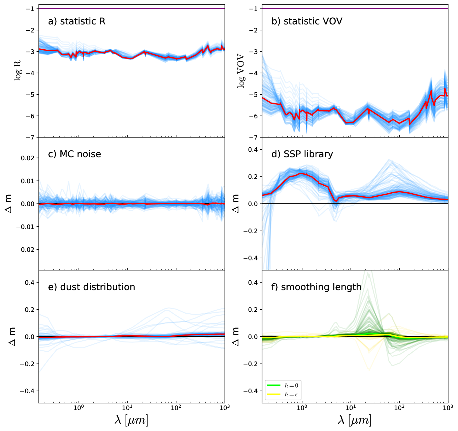
Figure 16: a) and b): Results of the statistical tests, the relative error R, and the variance of the variance VOV. c): Monte Carlo noise shown as the magnitude differences of the different bands for the two identical RT simulation runs. d), e) and f): Change in galaxy magnitudes due to the different SSP library, dust distribution and smoothing length, respectively. The blue (green/yellow for f) lines represent individual galaxies, and the red line is the median of the TNG50 sumbsample. The purple line in the top panels shows the reliability threshold.

Appendix C Comparison of physical properties

To validate our post processing procedure, we confront the true galaxy properties with those derived from the cigale SED fitting tool and from the common tracers.

C.1 cigale stellar mass and SFR

In Fig. 17 we analyse galaxy stellar mass (left) and SFR (right) for 136 galaxies of the TNG subsample. Both SFRs represent instantaneous SFRs. The different colours correspond to the different recipes considered in this study and mentioned in the main text. Increasing $\tau$ generally increases the spread in the relations, as the young stellar emission is being dimmed.

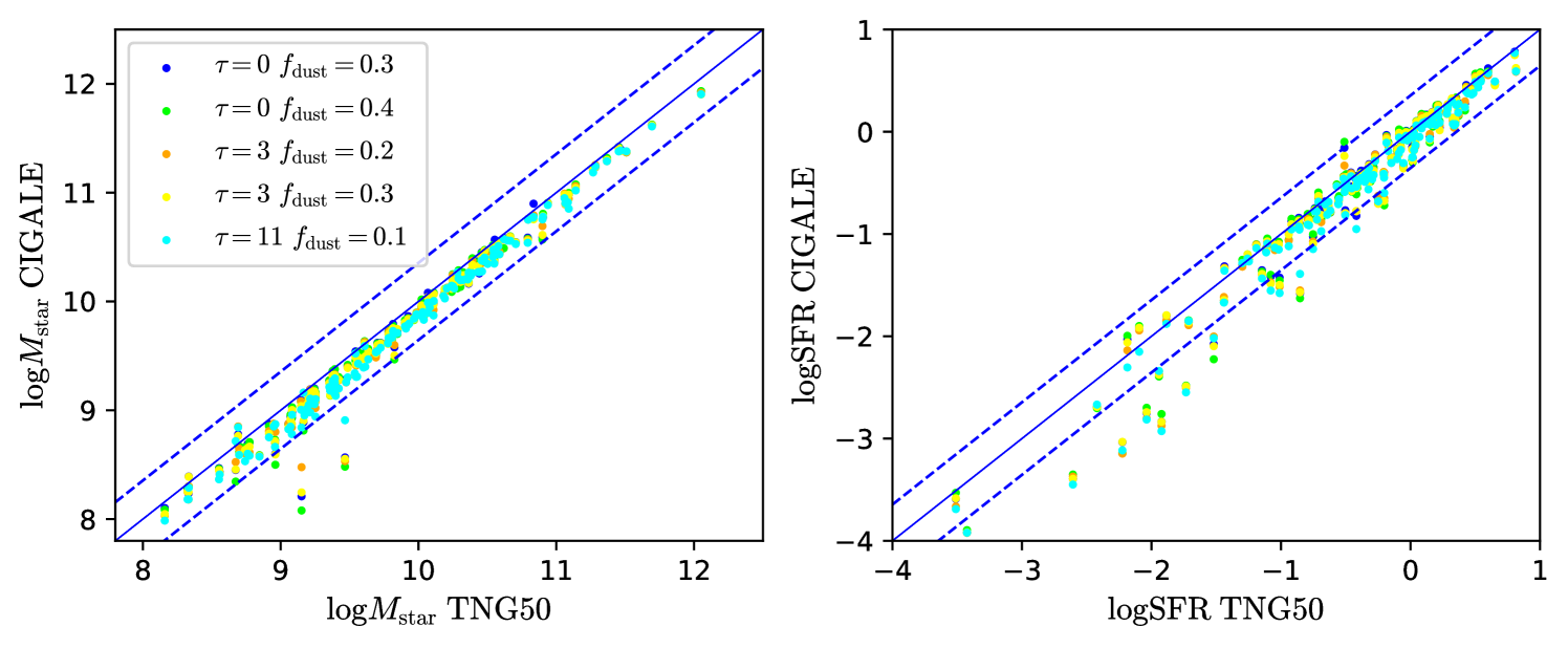
Figure 17: Comparison between $M_{\mathrm{star}}$ (left) and SFR (right) retrieved from the simulation data and from cigale, both inside $5\,R_{1/2}$, for different recipes. The blue solid line is one-to-one line, and the dashed lines represent $\pm 0.25\;\mathrm{dex}$ lines.

C.2 Stellar mass and SFR tracers

Here we explore how the intrinsic simulation properties correlate with the appropriate proxies from the literature. The results are shown in Fig. 18. For the $M_{\mathrm{star}}$ tracer we rely on the recipe from Taylor et al. (2011), based on the optical measurement i.e. $\log(M_{\mathrm{star}}/M_{\mathrm{\odot}})=1.15+0.7(g-i)-0.4M_{i}$. Other available recipes provide different scaling coefficients, and our results are within these uncertainties (Gallazzi & Bell, 2009; Zibetti et al., 2009; Roediger & Courteau, 2015). As a SFR proxy, the FUV band is the most common choice. We selected a dust-corrected recipe from Hao et al. (2011), which also includes MIPS 24 $\mu m$. Although this proxy traces longer-term SFR ($\sim$ 100 Myr Kennicutt & Evans, 2012), the agreement is outstanding. To check the difference between instantaneous and time-averaged SFR (over 100 Myr), we used the supplementary TNG50 catalogue (Donnari et al., 2019; Pillepich et al., 2019), and compared these SFRs within the aperture of $2R_{1/2}$. We found that the instantaneous SFR deviates from the time-averaged only in the low SFR regime and no more than 0.2 dex. Therefore, our SFR correlation would be even tighter if we had used time-averaged SFR. In the bottom left corner are the intrinsically passive galaxies where the MIPS 24 $\mu m$ emission is coming solely from the evolved stars. Most of them are predicted to have SFR not greater than $0.0001\mathrm{M_{\odot}yr^{-1}}$.

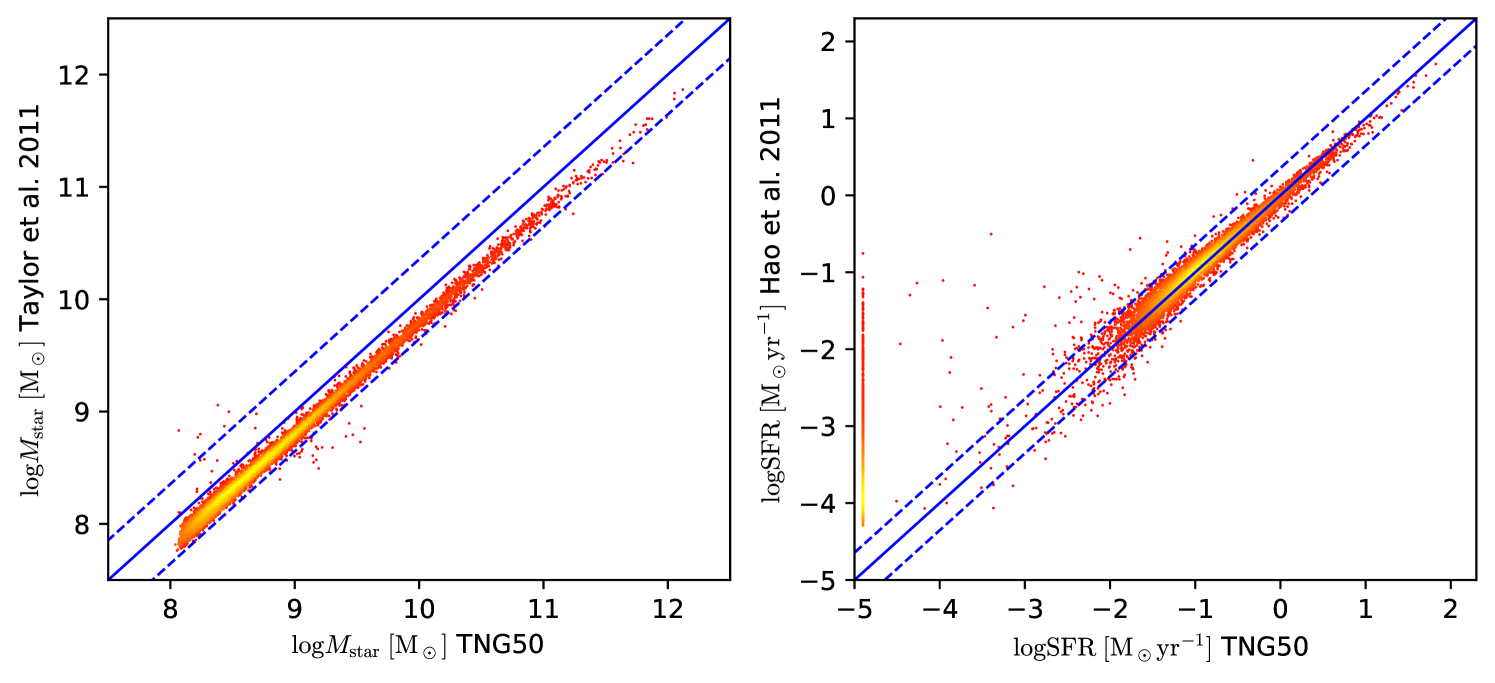
Figure 18: Comparison between $M_{\mathrm{star}}$ (left) and SFR (right) retrieved from the simulation data and from the fluxes, based on the recipe from the literature. The total TNG50 sample at $z=0$ is presented. The galaxies at the left corner of the SFR plot are those with intrinsically $\mathrm{SFR}=0$. The blue solid line is one-to-one line, and the dashed lines represent $\pm 0.25\;\mathrm{dex}$ lines.

Appendix D Broadband flux information

Table 2 displays the selection of publicly available bands derived for each TNG50 galaxy with $\log M_{\mathrm{star}}>8\;\mathrm{M_{\odot}}$.

Table 2: Available broadband fluxes. Survey, telescope or photometric system, band and its pivot wavelength.

Survey/System	Band	Pivot wavelength [$\mu m$]
GALEX	FUV	0.15
	NUV	0.23
Johnson	U	0.35
	B	0.44
	V	0.55
	R	0.69
	I	0.87
	J	1.24
	M	5.01
SDSS	u	0.36
	g	0.47
	r	0.62
	i	0.75
	z	0.89
UKIDSS	Z	0.88
	Y	1.03
	J	1.25
	H	1.64
	K	2.21
2MASS	J	1.24
	H	1.65
	Ks	2.16
WISE	1	3.39
	2	4.64
	3	12.6
	4	22.3
Spitzer	IRAC 1	3.55
	IRAC 2	4.50
	IRAC 3	5.72
	IRAC 4	7.88
	MIPS 24	23.8
	MIPS 70	72
	MIPS 160	156
IRAS	12	11.4
	25	23.6
	60	60.4
	100	101
Herschel	PACS 70	70.8
	PACS 100	101
	PACS 160	162
	SPIRE 250	253
	SPIRE 350	354
	SPIRE 500	515
JCMT	SCUBA2 450	449
	SCUBA2 850	854
Planck	857	352
	545	545
	353	839
ALMA	10	350
	9	456
	8	690
	7	938
	6	1244

Appendix E Aperture definition

To associate our aperture definitions with observational ones, we applied the statmorph package (Rodriguez-Gomez et al., 2019) on images in the SDSS $i$ band, and derived the Petrosian radii ($R_{\mathrm{petro}}$) for all the galaxies in our sample. In Fig. 19 we show how our fiducial aperture at $z=0$ correlates with $2\,R_{\mathrm{petro}}$, the aperture typically used in the literature. Focusing on the range above 10 kpc, we see how the Petrosian aperture is slightly smaller than the fiducial one (no more than 0.1 dex), but the apertures are tightly correlated. While it seems that the aperture of 10 kpc mostly resolves the discrepancy between the observed and simulated LFs at the bright end, we see from Fig. 19 that for large galaxies (which populate the bright end of the LFs), this aperture will probably capture less light. Instead, the aperture of 30 kpc is a better approximation, as also seen in Schaye et al. (2015); Pillepich et al. (2018b), although they applied it in 3D while we did in 2D (along the line of sight, the height of the cylinder is always $10\,R_{\mathrm{1/2}}$). They also focused on the larger simulation boxes, which include a higher number of the most massive/luminous galaxies.

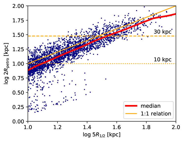
Figure 19: Correlation between our fiducial aperture (x-axis) and a Petrosian aperture, for a sub-sample of large TNG50 galaxies. The horizontal lines correspond to the 10 and 30 kpc apertures; the orange solid line is one-to-one relation and the red line is the running median.

References

- Baes & Camps (2015) Baes M., Camps P., 2015, Astronomy and Computing, 12, 33
- Baes et al. (2011) Baes M., Verstappen J., De Looze I., Fritz J., Saftly W., Vidal Pérez E., Stalevski M., Valcke S., 2011, ApJS, 196, 22
- Baes et al. (2016) Baes M., Gordon K. D., Lunttila T., Bianchi S., Camps P., Juvela M., Kuiper R., 2016, A&A, 590, A55
- Baes et al. (2019) Baes M., Trčka A., Camps P., Nersesian A., Trayford J., Theuns T., Dobbels W., 2019, MNRAS, 484, 4069
- Baes et al. (2020) Baes M., et al., 2020, MNRAS, 494, 2912
- Baldry et al. (2004) Baldry I. K., Balogh M. L., Bower R., Glazebrook K., Nichol R. C., 2004, in Allen R. E., Nanopoulos D. V., Pope C. N., eds, American Institute of Physics Conference Series Vol. 743, The New Cosmology: Conference on Strings and Cosmology. pp 106–119 (arXiv:astro-ph/0410603), doi:10.1063/1.1848322
- Bell et al. (2003) Bell E. F., McIntosh D. H., Katz N., Weinberg M. D., 2003, ApJS, 149, 289
- Bernardi et al. (2013) Bernardi M., Meert A., Sheth R. K., Vikram V., Huertas-Company M., Mei S., Shankar F., 2013, MNRAS, 436, 697
- Bianchi et al. (2018) Bianchi S., et al., 2018, A&A, 620, A112
- Blanton et al. (2003) Blanton M. R., et al., 2003, ApJ, 592, 819
- Boquien et al. (2019) Boquien M., Burgarella D., Roehlly Y., Buat V., Ciesla L., Corre D., Inoue A. K., Salas H., 2019, A&A, 622, A103
- Boselli et al. (2010) Boselli A., et al., 2010, PASP, 122, 261
- Bruzual & Charlot (2003) Bruzual G., Charlot S., 2003, Mon. Not. R. Astron. Soc., 344, 1000
- Budavári et al. (2005) Budavári T., et al., 2005, ApJ, 619, L31
- Calzetti et al. (2000) Calzetti D., Armus L., Bohlin R. C., Kinney A. L., Koornneef J., Storchi-Bergmann T., 2000, ApJ, 533, 682
- Camps & Baes (2015) Camps P., Baes M., 2015, Astronomy and Computing, 9, 20
- Camps & Baes (2020) Camps P., Baes M., 2020, Astronomy and Computing, 31, 100381
- Camps et al. (2013) Camps P., Baes M., Saftly W., 2013, A&A, 560, A35
- Camps et al. (2016) Camps P., Trayford J. W., M., Theuns T., Schaller M., Schaye J., 2016, MNRAS, 462, 1057
- Camps et al. (2018) Camps P., et al., 2018, Astrophys. J. Suppl. Ser., 234, 20
- Camps et al. (2022) Camps P., Kapoor A. U., Trčka A., Font A. S., McCarthy I. G., Trayford J., Baes M., 2022, arXiv e-prints, p. arXiv:2203.06078
- Casasola et al. (2017) Casasola V., et al., 2017, A&A, 605, A18
- Casey et al. (2014) Casey C. M., Narayanan D., Cooray A., 2014, Phys. Rep., 541, 45
- Chabrier (2003) Chabrier G., 2003, PASP, 115, 763
- Charlot & Fall (2000) Charlot S., Fall S. M., 2000, ApJ, 539, 718
- Ciesla et al. (2016) Ciesla L., et al., 2016, A&A, 585, A43
- Clark et al. (2018) Clark C. J. R., et al., 2018, A&A, 609, A37
- Cortese et al. (2012) Cortese L., et al., 2012, A&A, 540, A52
- Crain et al. (2015) Crain R. A., et al., 2015, MNRAS, 450, 1937
- Davé et al. (2019) Davé R., Anglés-Alcázar D., Narayanan D., Li Q., Rafieferantsoa M. H., Appleby S., 2019, MNRAS, 486, 2827
- Davies et al. (2017) Davies J. I., et al., 2017, Publ. Astron. Soc. Pacific, 129, 44102
- Davies et al. (2019) Davies J. I., et al., 2019, A&A, 626, A63
- De Cia et al. (2013) De Cia A., Ledoux C., Savaglio S., Schady P., Vreeswijk P. M., 2013, A&A, 560, A88
- De Vis et al. (2019) De Vis P., et al., 2019, A&A, 623, A5
- Dickey et al. (2021) Dickey C. M., et al., 2021, ApJ, 915, 53
- Donnari et al. (2019) Donnari M., et al., 2019, MNRAS, 485, 4817
- Donnari et al. (2021) Donnari M., Pillepich A., Nelson D., Marinacci F., Vogelsberger M., Hernquist L., 2021, MNRAS, 506, 4760
- Driver et al. (2011) Driver S. P., et al., 2011, MNRAS, 413, 971
- Driver et al. (2012) Driver S. P., et al., 2012, MNRAS, 427, 3244
- Duarte-Cabral & Dobbs (2017) Duarte-Cabral A., Dobbs C. L., 2017, MNRAS, 470, 4261
- Dubois et al. (2014) Dubois Y., et al., 2014, MNRAS, 444, 1453
- Dunne et al. (2011) Dunne L., et al., 2011, MNRAS, 417, 1510
- Eales et al. (2010) Eales S., et al., 2010, PASP, 122, 499
- Engler et al. (2021) Engler C., et al., 2021, MNRAS, 500, 3957
- Fasano & Franceschini (1987) Fasano G., Franceschini A., 1987, Monthly Notices of the Royal Astronomical Society, 225, 155
- Font et al. (2020) Font A. S., et al., 2020, MNRAS, 498, 1765
- Galametz et al. (2013) Galametz M., et al., 2013, MNRAS, 431, 1956
- Gallazzi & Bell (2009) Gallazzi A., Bell E. F., 2009, ApJS, 185, 253
- Galliano et al. (2021) Galliano F., et al., 2021, A&A, 649, A18
- Geha et al. (2012) Geha M., Blanton M. R., Yan R., Tinker J. L., 2012, ApJ, 757, 85
- Genel et al. (2014) Genel S., et al., 2014, MNRAS, 445, 175
- Genel et al. (2015) Genel S., Fall S. M., Hernquist L., Vogelsberger M., Snyder G. F., Rodriguez-Gomez V., Sijacki D., Springel V., 2015, ApJ, 804, L40
- Graham & Driver (2005) Graham A. W., Driver S. P., 2005, Publ. Astron. Soc. Australia, 22, 118
- Granato et al. (2021) Granato G. L., et al., 2021, MNRAS, 503, 511
- Grand et al. (2017) Grand R. J. J., et al., 2017, MNRAS, 467, 179
- Groves et al. (2008) Groves B., Dopita M., Sutherland R., Kewley L., Fischera J., Leitherer C., Brandl B., van Breugal W., 2008, Astrophys. J. Suppl. Ser., 176, 438
- Guedes et al. (2011) Guedes J., Callegari S., Madau P., Mayer L., 2011, ApJ, 742, 76
- Hahn et al. (2021) Hahn C., et al., 2021, arXiv e-prints, p. arXiv:2106.09741
- Hao et al. (2011) Hao C.-N., Kennicutt R. C., Johnson B. D., Calzetti D., Dale D. A., Moustakas J., 2011, ApJ, 741, 124
- Hayward et al. (2021) Hayward C. C., et al., 2021, MNRAS, 502, 2922
- Hill et al. (2010) Hill D. T., Driver S. P., Cameron E., Cross N., Liske J., Robotham A., 2010, MNRAS, 404, 1215
- Hill et al. (2011) Hill D. T., et al., 2011, MNRAS, 412, 765
- Hoffmann et al. (2020) Hoffmann K., Laigle C., Chisari N. E., Tallada P., Dubois Y., Devriendt J., 2020, arXiv e-prints, p. arXiv:2010.13845
- Huertas-Company et al. (2019) Huertas-Company M., et al., 2019, MNRAS, 489, 1859
- Jones et al. (2017) Jones A. P., Köhler M., Ysard N., Bocchio M., Verstraete L., 2017, A&A, 602, A46
- Jonsson et al. (2010) Jonsson P., Groves B. A., Cox T. J., 2010, MNRAS, 403, 17
- Joshi et al. (2021) Joshi G. D., Pillepich A., Nelson D., Zinger E., Marinacci F., Springel V., Vogelsberger M., Hernquist L., 2021, MNRAS, 508, 1652
- Kannan et al. (2020) Kannan R., Marinacci F., Vogelsberger M., Sales L. V., Torrey P., Springel V., Hernquist L., 2020, MNRAS, 499, 5732
- Kannan et al. (2021) Kannan R., Vogelsberger M., Marinacci F., Sales L. V., Torrey P., Hernquist L., 2021, MNRAS, 503, 336
- Kapoor et al. (2021) Kapoor A. U., et al., 2021, MNRAS, 506, 5703
- Kaviraj et al. (2017) Kaviraj S., et al., 2017, MNRAS, 467, 4739
- Kelvin et al. (2014) Kelvin L. S., et al., 2014, MNRAS, 439, 1245
- Kennicutt & Evans (2012) Kennicutt R. C., Evans N. J., 2012, ARA&A, 50, 531
- Kim & Ostriker (2017) Kim C.-G., Ostriker E. C., 2017, ApJ, 846, 133
- Kolmogorov (1933) Kolmogorov A., 1933, Giorn. Ist. Ital. Attuar., 4, 83
- Kron (1980) Kron R. G., 1980, ApJS, 43, 305
- Kroupa (2001) Kroupa P., 2001, MNRAS, 322, 231
- Lan et al. (2016) Lan T.-W., Ménard B., Mo H., 2016, MNRAS, 459, 3998
- Lawrence et al. (2007) Lawrence A., et al., 2007, MNRAS, 379, 1599
- Leitherer et al. (1999) Leitherer C., et al., 1999, ApJS, 123, 3
- Liske et al. (2003) Liske J., Lemon D. J., Driver S. P., Cross N. J. G., Couch W. J., 2003, MNRAS, 344, 307
- Liske et al. (2015) Liske J., et al., 2015, MNRAS, 452, 2087
- Lo Faro et al. (2017) Lo Faro B., Buat V., Roehlly Y., Alvarez-Marquez J., Burgarella D., Silva L., Efstathiou A., 2017, MNRAS, 472, 1372
- Loveday et al. (2012) Loveday J., et al., 2012, MNRAS, 420, 1239
- Lovell et al. (2021) Lovell C. C., Geach J. E., Davé R., Narayanan D., Coppin K. E. K., Li Q., Franco M., Privon G. C., 2021, arXiv e-prints, p. arXiv:2106.11588
- Ma et al. (2019) Ma X., et al., 2019, MNRAS, 487, 1844
- Marchetti et al. (2016) Marchetti L., et al., 2016, MNRAS, 456, 1999
- Marinacci et al. (2018) Marinacci F., et al., 2018, MNRAS, 480, 5113
- McKinnon et al. (2018) McKinnon R., Vogelsberger M., Torrey P., Marinacci F., Kannan R., 2018, MNRAS, 478, 2851
- Millard et al. (2021) Millard J. S., Diemer B., Eales S. A., Gomez H. L., Beeston R., Smith M. W. L., 2021, MNRAS, 500, 871
- Mitchell et al. (2013) Mitchell P. D., Lacey C. G., Baugh C. M., Cole S., 2013, MNRAS, 435, 87
- Mitchell et al. (2021) Mitchell M. A., Arnold C., Li B., 2021, arXiv e-prints, p. arXiv:2109.01147
- Morrissey et al. (2007) Morrissey P., et al., 2007, ApJS, 173, 682
- Mosenkov et al. (2019) Mosenkov A. V., et al., 2019, A&A, 622, A132
- Naiman et al. (2018) Naiman J. P., et al., 2018, MNRAS, 477, 1206
- Narayanan et al. (2018) Narayanan D., Conroy C., Davé R., Johnson B. D., Popping G., 2018, ApJ, 869, 70
- Negrello et al. (2013) Negrello M., et al., 2013, MNRAS, 429, 1309
- Nelson et al. (2018) Nelson D., et al., 2018, MNRAS, 475, 624
- Nelson et al. (2019a) Nelson D., et al., 2019a, Computational Astrophysics and Cosmology, 6, 2
- Nelson et al. (2019b) Nelson D., et al., 2019b, MNRAS, 490, 3234
- Nersesian et al. (2019) Nersesian A., et al., 2019, A&A, 624, A80
- Nguyen et al. (2010) Nguyen H. T., et al., 2010, A&A, 518, L5
- Norris et al. (2014) Norris M. A., Meidt S., Van de Ven G., Schinnerer E., Groves B., Querejeta M., 2014, ApJ, 797, 55
- Oliver et al. (2012) Oliver S. J., et al., 2012, MNRAS, 424, 1614
- Peacock (1983) Peacock J. A., 1983, Monthly Notices of the Royal Astronomical Society, 202, 615
- Peng et al. (2010) Peng Y.-j., et al., 2010, ApJ, 721, 193
- Péroux & Howk (2020) Péroux C., Howk J. C., 2020, ARA&A, 58, 363
- Petrosian (1976) Petrosian V., 1976, ApJ, 210, L53
- Pillepich et al. (2018a) Pillepich A., et al., 2018a, MNRAS, 473, 4077
- Pillepich et al. (2018b) Pillepich A., et al., 2018b, MNRAS, 475, 648
- Pillepich et al. (2019) Pillepich A., et al., 2019, MNRAS, 490, 3196
- Planck Collaboration et al. (2011) Planck Collaboration et al., 2011, A&A, 536, A7
- Planck Collaboration et al. (2016) Planck Collaboration et al., 2016, A&A, 594, A13
- Popping et al. (2022) Popping G., et al., 2022, MNRAS, 510, 3321
- Rémy-Ruyer et al. (2014) Rémy-Ruyer A., et al., 2014, A&A, 563, A31
- Rigby et al. (2011) Rigby E. E., et al., 2011, MNRAS, 415, 2336
- Rodriguez-Gomez et al. (2019) Rodriguez-Gomez V., et al., 2019, MNRAS, 483, 4140
- Roediger & Courteau (2015) Roediger J. C., Courteau S., 2015, MNRAS, 452, 3209
- Saftly et al. (2013) Saftly W., Camps P., Baes M., Gordon K. D., Vandewoude S., Rahimi A., Stalevski M., 2013, A&A, 554, A10
- Saftly et al. (2014) Saftly W., Baes M., Camps P., 2014, A&A, 561, A77
- Saftly et al. (2015) Saftly W., Baes M., De Geyter G., Camps P., Renaud F., Guedes J., De Looze I., 2015, A&A, 576, A31
- Salim (2014) Salim S., 2014, Serbian Astronomical Journal, 189, 1
- Salpeter (1955) Salpeter E. E., 1955, ApJ, 121, 161
- Sawala et al. (2016) Sawala T., et al., 2016, MNRAS, 457, 1931
- Schaye et al. (2015) Schaye J., et al., 2015, MNRAS, 446, 521
- Schulz et al. (2020) Schulz S., Popping G., Pillepich A., Nelson D., Vogelsberger M., Marinacci F., Hernquist L., 2020, MNRAS, 497, 4773
- Seifried et al. (2018) Seifried D., Walch S., Haid S., Girichidis P., Naab T., 2018, ApJ, 855, 81
- Shen et al. (2021) Shen X., Vogelsberger M., Nelson D., Tacchella S., Hernquist L., Springel V., Marinacci F., Torrey P., 2021, arXiv e-prints, p. arXiv:2104.12788
- Smirnov (1948) Smirnov N., 1948, Ann. Math. Statist., 19, 279
- Smith et al. (2020) Smith R. J., et al., 2020, MNRAS, 492, 1594
- Smith et al. (2021) Smith A., et al., 2021, arXiv e-prints, p. arXiv:2111.13721
- Springel (2010) Springel V., 2010, MNRAS, 401, 791
- Springel & Hernquist (2003) Springel V., Hernquist L., 2003, MNRAS, 339, 289
- Springel et al. (2018) Springel V., et al., 2018, MNRAS, 475, 676
- Sullivan et al. (2000) Sullivan M., Treyer M. A., Ellis R. S., Bridges T. J., Milliard B., Donas J., 2000, MNRAS, 312, 442
- Tacchella et al. (2022) Tacchella S., et al., 2022, MNRAS,
- Tang et al. (2021) Tang L., Lin W., Wang Y., Napolitano N. R., 2021, MNRAS, 508, 3321
- Taylor et al. (2011) Taylor E. N., et al., 2011, MNRAS, 418, 1587
- Taylor et al. (2015) Taylor E. N., et al., 2015, MNRAS, 446, 2144
- Torrey et al. (2012) Torrey P., Vogelsberger M., Sijacki D., Springel V., Hernquist L., 2012, MNRAS, 427, 2224
- Torrey et al. (2015) Torrey P., et al., 2015, MNRAS, 447, 2753
- Torrey et al. (2019) Torrey P., et al., 2019, MNRAS, 484, 5587
- Trayford et al. (2015) Trayford J. W., et al., 2015, MNRAS, 452, 2879
- Trayford et al. (2017) Trayford J. W., et al., 2017, Mon. Not. R. Astron. Soc., 470, 771
- Trayford et al. (2019) Trayford J. W., Frenk C. S., Theuns T., Schaye J., Correa C., 2019, MNRAS, 483, 744
- Trayford et al. (2020) Trayford J. W., Lagos C. d. P., Robotham A. S. G., Obreschkow D., 2020, MNRAS, 491, 3937
- Tremmel et al. (2019) Tremmel M., et al., 2019, MNRAS, 483, 3336
- Trčka et al. (2020) Trčka A., et al., 2020, MNRAS, 494, 2823
- Utomo et al. (2019) Utomo D., Chiang I.-D., Leroy A. K., Sandstrom K. M., Chastenet J., 2019, ApJ, 874, 141
- Vaccari (2015) Vaccari M., 2015, in Proceedings of “The many facets of extragalactic radio surveys: towards new scientific challenges” (EXTRA-RADSUR2015). 20-23 October 2015. Bologna. p. 27 (arXiv:1604.02353)
- Vaccari et al. (2010) Vaccari M., et al., 2010, A&A, 518, L20
- Vandenbroucke et al. (2021) Vandenbroucke B., Baes M., Camps P., Utsav Kapoor A., Barrientos D., Bernard J.-P., 2021, arXiv e-prints, p. arXiv:2107.02180
- Verstocken et al. (2017) Verstocken S., Van De Putte D., Camps P., Baes M., 2017, Astronomy and Computing, 20, 16
- Viaene et al. (2016) Viaene S., et al., 2016, A&A, 586, A13
- Vogelsberger et al. (2014a) Vogelsberger M., et al., 2014a, MNRAS, 444, 1518
- Vogelsberger et al. (2014b) Vogelsberger M., et al., 2014b, Nature, 509, 177
- Vogelsberger et al. (2018) Vogelsberger M., et al., 2018, MNRAS, 474, 2073
- Vogelsberger et al. (2020a) Vogelsberger M., Marinacci F., Torrey P., Puchwein E., 2020a, Nature Reviews Physics, 2, 42
- Vogelsberger et al. (2020b) Vogelsberger M., et al., 2020b, MNRAS, 492, 5167
- Weinberger et al. (2017) Weinberger R., et al., 2017, MNRAS, 465, 3291
- Wetzel et al. (2016) Wetzel A. R., Hopkins P. F., Kim J.-h., Faucher-Giguère C.-A., Kereš D., Quataert E., 2016, ApJ, 827, L23
- Wyder et al. (2005) Wyder T. K., et al., 2005, ApJ, 619, L15
- York et al. (2000) York D. G., et al., 2000, AJ, 120, 1579
- Yuan et al. (2021) Yuan F.-T., Lu J., Shen S., Boquien M., 2021, ApJ, 911, 145
- Zabel et al. (2021) Zabel N., et al., 2021, MNRAS, 502, 4723
- Zafar & Watson (2013) Zafar T., Watson D., 2013, A&A, 560, A26
- Zibetti et al. (2009) Zibetti S., Charlot S., Rix H.-W., 2009, MNRAS, 400, 1181
- Zubko et al. (2004) Zubko V., Dwek E., Arendt R. G., 2004, ApJS, 152, 211