Deep learning automates bidimensional and volumetric tumor burden measurement from MRI in pre- and post-operative glioblastoma patients

Abstract

Tumor burden assessment by magnetic resonance imaging (MRI) is central to the evaluation of treatment response for glioblastoma. This assessment is complex to perform and associated with high variability due to the high heterogeneity and complexity of the disease. In this work, we tackle this issue and propose a deep learning pipeline for the fully automated end-to-end analysis of glioblastoma patients. Our approach simultaneously identifies tumor sub-regions, including the enhancing tumor, peritumoral edema and surgical cavity in the first step, and then calculates the volumetric and bidimensional measurements that follow the current Response Assessment in Neuro-Oncology (RANO) criteria. Also, we introduce a rigorous manual annotation process which was followed to delineate the tumor sub-regions by the human experts, and to capture their segmentation confidences that are later used while training the deep learning models. The results of our extensive experimental study performed over 760 pre-operative and 504 post-operative adult patients with glioma obtained from the public database (acquired at 19 sites in years 2021–2020) and from a clinical treatment trial (47 and 69 sites for pre-/post-operative patients, 2009–2011) and backed up with thorough quantitative, qualitative and statistical analysis revealed that our pipeline performs accurate segmentation of pre- and post-operative MRIs in a fraction of the manual delineation time (up to 20 times faster than humans). The bidimensional and volumetric measurements were in strong agreement with expert radiologists, and we showed that RANO measurements are not always sufficient to quantify tumor burden.

1 Introduction

Glioblastoma (GBM) is the most common of malignant primary brain tumors in adults and despite decades of research, still remains one of the most feared of all cancer types due to its poor prognosis. Accurately evaluating response to therapies in GBM also presents considerable challenges. It is based on the use of the Response Assessment in Neuro-Oncology (RANO) criteria and the measurement of two perpendicular diameters of the contrast-enhancing tumor (ET) area [Ellingson et al., 2017], as well as a qualitative evaluation of abnormalities on T2-weighted and FLAIR MRI sequences, which correspond to regions of edema (ED) with or without tumor cell infiltration. Radiological evaluation is notoriously complex as the tumors are often very heterogeneous in appearance, with an irregular shape associated with the infiltrative nature of the disease. The effect is further compounded in the post-surgical setting, by the presence of the surgical cavity and brain distortion. Inevitably, this leads to high intra- and inter-reader variability which, in turn, limits our ability to detect a therapeutic benefit in clinical trials and capture early patient response or progression in clinical practice. In this work, we tackle this issue and propose an end-to-end deep learning pipeline for the segmentation of tumor sub-regions from MRI for patients with glioma and the subsequent automated measurements of their volumetric characteristics and bidimensional diameters—our most important contributions are summarized in Section 1.2, whereas Section 1.1 presents the related literature.

1.1 Related literature

Segmentation of glioblastoma (former name: glioblastoma multiforme) from multi-sequence MRI scans has been extensively researched in the literature [Bakas et al., 2018, Nalepa et al., 2020], and it was popularized by the Brain Tumor Segmentation (BraTS) challenge that is focusing on developing automated algorithms for accurate brain tumor multi-class segmentation [Menze et al., 2015, Baid et al., 2021]. The existing algorithms targeting the brain tumor detection and segmentation are commonly split into three main categories [Liu et al., 2014, Wadhwa et al., 2019]—(i) atlas-, (ii) image analysis-, and (iii) machine learning-based techniques. Such approaches may be also assembled into hybrid techniques which benefit from the advantages of the combined algorithms [Zhao et al., 2018, Habib et al., 2021, Kadry et al., 2021].

The atlas-based models [Visser et al., 2020], that span across single- and multi-atlas label propagation techniques, segment the input MRI scans by extrapolating them to the previously curated reference images (referred to as atlases) that represent the natural anatomical variability of the brain tissue [Park et al., 2014]. This is often a two-step process involving the global image registration that initially aligns the scans, and fine-tuning that captures local adaptations to specific brain anatomies (there exist methods that combine non-rigid registration with various tumor growth models [Bauer et al., 2010]). Therefore, the overall quality of tumor segmentation is directly influenced by the representativeness of the utilized atlases (which are not necessarily transferable across scans of different characteristics [Aljabar et al., 2009]) and the performance of the co-registration process, thus developing well-performing deformable image registration techniques is of high practical importance in this context [Mohamed et al., 2006]. The latter approaches can also lead to non-rigid transformations which are not necessarily anatomically plausible, especially in the case of deformed brains [Nalepa et al., 2020]. Such methods are, however, easy to parallelize and interpret, but require building comprehensive atlases in the cumbersome, costly, and user-dependent process. This procedure could be accelerated through employing semi-automated techniques [Sagberg et al., 2019], especially in specific scenarios, e.g., for post-operative patients with affected brain anatomies.

Classical image analysis algorithms are usually classified into (i) the approaches that label the voxels based on their intensity through employing various (single- and multi-level [Al-Rahlawee and Rahebi, 2021]) thresholding approaches [Ilhan and Ilhan, 2017] or (ii) the algorithms that analyze the characteristics of the voxel’s neighborhood in a region-based manner. The former techniques offer real-time operation and are trivial to implement, but the appropriate threshold values should be either fine-tuned beforehand, or dynamically selected based on the input MRI characteristics. Additionally, since the brain tumors may manifest significant intensity variations, thresholding-based approaches can fail for heterogeneous lesions, and are susceptible to image noise, hence commonly require additional de-noising [Sharif et al., 2018]. On the other hand, exploiting the neighborhood voxel’s information can robustify such techniques through extracting hand-crafted features. In region growing algorithms, the input scan is split into coherent regions, according to specific similarity metrics that should be selected a priori [Srinivasa Reddy and Chenna Reddy, 2021]. In the active contour approaches, the initially determined contours are evolved toward the exact tumor boundaries [Essadike et al., 2018]. Such techniques track the tumor boundaries through matching a deformable model to the object (lesion), according to the energy functional that effectively controls the rigidity and elasticity of the curve [Ben Rabeh et al., 2017, Meng et al., 2017]. Although being thoroughly researched in the computer vision and medical image analysis fields, active contour techniques are still heavily parameterized and do not perform well in the case of sharp corners, concavities, and smooth boundaries [Nalepa et al., 2020]. They are, however, commonly used in semi-supervised segmentation pipelines, in which practitioners can provide valid initial contouring and parameterizations of the deformable model [Nakhmani et al., 2014].

Machine learning approaches for brain tumor segmentation are split into the (i) conventional techniques which require manual feature engineering, including feature extraction often followed by feature selection which aims at determining a subset of the most discriminative image features [Poernama et al., 2019, Varuna Shree and Kumar, 2018, Abbas et al., 2021], and (ii) deep learning algorithms that learn features from the data automatically during the training process, hence benefit from automated representation learning [Naser and Deen, 2020]. In unsupervised segmentation algorithms [Wu et al., 2021], we do not exploit manually-delineated training sets, but utilize the data characteristics—captured in the input or specific feature spaces [Yu et al., 2021]—to partition the image data into consistent clusters of voxels [Chen et al., 2018, Wu et al., 2021]. Unsupervised segmentation can be conveniently exploited as a pre-processing step, e.g., while generating ground-truth examples that could be later used for training supervised learners, as the pre-segmented MRI scans are much faster to analyze, interpret, and ultimately annotate by human readers. This partial automation which is offered by unsupervised learning has been recently used in the unsupervised quality control of segmentations, where the quality estimates are produced by comparing each segmentation with the output of a probabilistic segmentation model that relies on certain intensity and smoothness assumptions. Here, unsupervised approach helps determine atypical segmentation maps, and even predict the performance of segmentation algorithms [Audelan and Delingette, 2021]. On the other hand, supervised learners utilize the ground-truth delineations in the training process. Such algorithms span across numerous well-established and widely utilized classification engines, and include, among others, support vector machines [Mishra and Deepthi, 2021], random forests [Lefkovits et al., 2016], $k$-nearest neighbor ($k$-NN) classifiers [Kirtania et al., 2020], extreme learning machines [Sasank and Venkateswarlu, 2021], ensemble learners [Barzegar and Jamzad, 2020], and others [Seo et al., 2020]. Although some of the aforementioned models are trivial to interpret, e.g., $k$-NNs, it is not the case for non-linear algorithms which additionally require fine-tuning their pivotal hyper-parameters, and they can be sensitive to noise in the training sample. Therefore, selecting appropriate training sets can play a critical role in elaborating well-generalizing machine learning models [Nalepa and Kawulok, 2019].

Currently, deep learning has been blooming in the field of automatic analysis of medical image data, and has established the state of the art in numerous segmentation tasks through delivering the winning solutions in the recent biomedical segmentation competitions [Isensee et al., 2021a, Saleem et al., 2021]. Automated representation learning that underpins the deep learning algorithms allows us to reveal features that may be impossible to capture by humans—there have been a multitude of deep architectures proposed so far for automating the process of brain tumor contouring. Such approaches include a variety of convolutional neural networks [Ben naceur et al., 2020, Wang et al., 2019], generative adversarial models [Yuan et al., 2020], residual architectures [Saha et al., 2021], context-aware models [Pei et al., 2020], inception-based networks [Cahall et al., 2019], and many more [Tajbakhsh et al., 2020], but the recent BraTS editions clearly indicate that the U-Net-based [Ronneberger et al., 2015] architectures outperform other approaches for this task. The variations of this encoder-decoder model encompass multi-level cascaded techniques which sequentially detect whole-tumor areas, and then segment specific types of the brain tumor tissue [Kotowski et al., 2020], lightweight U-Nets [Tarasiewicz et al., 2020], the U-Nets with various loss functions, also capturing the boundary tumor’s characteristics [Lorenzo et al., 2019], hardware-optimized models [Xiong et al., 2021], hybrid algorithms that combine U-Nets with densely-connected and residual architectures [Zeineldin et al., 2020], ensembled U-Nets [Zhang et al., 2021c], and many more [Aboelenein et al., 2020, Hu et al., 2021, Zhang et al., 2021a, b]. Building a new deep learning algorithm for a given task requires defining not only the network’s architecture, but also its most hyper-parameters [Lorenzo et al., 2017], such as its depth, number and size of kernels, data augmentation routines executed to synthesize training data if necessary [Nalepa et al., 2019b, Shorten and Khoshgoftaar, 2019, Nalepa et al., 2019a], pre- and post-processing operations, or training strategy. Isensee et al. [2021a] approached this issue and introduced the nnU-Net framework that allows us to automatically optimize U-Net-based models for medical image segmentation. The recent BraTS editions showed that nnU-Nets became the model of choice for accurate brain tumor segmentation—they not only won BraTS 2020 with a significant margin [Isensee et al., 2021b] (and other biomedical challenges [Isensee et al., 2021a]), but are commonly deployed in emerging algorithms. In this work, we follow this research pathway and build upon the nnU-Net framework and extend it through the exploitation of the radiologists’ confidence concerning their manual annotations during the training process. Of note, we have thoroughly investigated 34 deep learning architectures to fully understand the impact of the most important architectural choices, together with the selection of training data on the abilities of the U-Net algorithms.

Overall, there exist a plethora of brain tumor delineation algorithms, but segmentation is virtually never the final step in the processing chain—the segmented areas are further analyzed to extract quantifiable tumor’s characteristics (thus, inaccurate segmentation will directly affect the quality of all other steps). However, manual analysis if often affected by the subjectivity of the rater leading to high intra- and inter-rater variability [Crowe et al., 2017, Visser et al., 2019], which adversely impact our capabilities of objectively monitoring the patient’s response to the treatment in longitudinal studies, clinical trials, and multi-center investigations. Therefore, automating the entire analysis chain is of utmost practical importance, as it could allow us to extract patient-specific information in a fully reproducible and unbiased way [Nalepa et al., 2020]. Virtually all computer-assisted methods that target GBM patients exploit semi-automated techniques [Egger et al., 2013], in which—although significantly accelerated—the interaction with the user is still an important factor affecting quality and reproducibility of the calculated measures, e.g., volumetric tumor’s characteristics [Chow et al., 2014, Sezer et al., 2020]. Meier et al. [2017] showed that automatic estimation of extent of resection and residual tumor volume of patients with GBM are comparable to the estimates of human experts, but commonly lead to overestimated volumes. The end-to-end fully-automated pipeline that we propose in this paper builds upon the pioneering work done by Chang et al. [2019] in post-operative GBM, recently used in pediatric brain tumors [Peng et al., 2021], with significant improvements that allow us to address the limitations of the aforementioned work, and related to the segmentation and RANO bidimensional calculation algorithms, clinical data preparation, assessment and utilization, and finally verification over a large and heterogeneous multi-center clinical data (the detailed comparison with Chang et al. [2019] is given in the Supplementary Material). To our knowledge, the work presented here is the first reported deep learning algorithm capable of identifying and segmenting multiple tumor areas for both pre and post-surgery patients with glioma. Additionally, it objectively assesses the tumorous regions by extracting their quantifiable volumetric and bidimensional characteristics.

1.2 Contribution

In this paper, we report on our effort to ease the radiological interpretation of the disease with the development of an end-to-end deep learning pipeline for the segmentation of brain tumors and subsequent automated measurements of their volumes and bidimensional diameters. We thoroughly investigate the performance of our technique and its ability to discriminate and quantify tumor sub-regions in pre-surgery as well as in post-surgery settings by comparing the automated assessment to the results obtained by expert radiologists. Overall, our contributions are multi-fold and can be summarized by the following bullet points:

• We propose an end-to-end pipeline for the simultaneous segmentation of the brain tumor sub-regions (enhancing tumor, peritumoral edema and surgical cavity) from multi-modal MRI (Section 2.3). The proposed approach benefits from the recent advances in the deep learning field and builds upon and extends the nnU-Net engine which established the state of the art in the medical image segmentation for a variety of organs and modalities [Isensee et al., 2021a, Saleem et al., 2021]. Once the sub-regions are delineated, we automatically measure the bidimensional and volumetric characteristics of the tumor, according to the current RANO criteria. Additionally, we introduce a new way of calculating RANO which is less sensitive to small alterations in the contour of the lesions, hence more robust against varying-quality automated segmentations and jagged contouring.

• We introduce a rigorous manual annotation procedure (Section 2.2) and follow it in this work to ensure the high quality of manual delineations, and to capture additional information related to the segmentation process, including the time of manual analysis alongside the readers’ confidences concerning each tumor sub-region. The confidences are utilized in the proposed confidence-aware nnU-Nets during their training process.

• We perform an extensive multi-fold experimental validation of the proposed pipeline in order to fully understand and quantify its capabilities in a range of clinical settings (Section 3). We utilized 760 pre-operative and 504 post-operative MRIs captured in dozens of institutions, therefore they manifest high level of data heterogeneity (Section 2.1). The experimental results indicate that the algorithm is able to analyze MRI scans for both pre-operative and post-operative patients producing results that are often more consistent, accurate and reliable than human experts in a fraction of time required by expert radiologists (up to 20$\times$ faster). To our knowledge, our technique is the first in the literature that effectively targets both pre- and post-operative MRIs using a single deep learning algorithm, and has been validated over a large and heterogeneous set of MRI data.

2 Materials and methods

2.1 Patient cohorts

We collected five cohorts of adult patients with glioma consisting of MRI visits either in pre-surgery (4 cohorts) or post-surgery setting (1 cohort) (Table 1). The Brain Tumor Segmentation (BraTS 2020) pre-operative cohorts consisted of 660 patients with pre-operative MRI scans of GBM/high-grade gliomas (HGGs) and low-grade gliomas (LGGs) with pathologically confirmed diagnosis, captured in 19 institutions using different equipment and imaging protocols (years 2012–2020) [Bakas et al., 2017a, b, c, Menze et al., 2015]. This dataset was divided into a training set BraTS 2020 (Tr) of 369 patients, a validation set BraTS 2020 (V) of 125 patients and a test set BraTS 2020 (Te) of 166 patients—the brain tumor labels are publicly available only for BraTS 2020 (Tr). To the best of our knowledge, BraTS is the largest and the most comprehensive public domain GBM MRI dataset (in terms of types of utilized scanners, imaging protocols and types of imaged lesions) currently available for validating emerging tumor segmentation algorithms, such as within the framework of the Brain Tumor Segmentation Challenge organized yearly [Bakas et al., 2018, Baid et al., 2021]. The MRIs include the native T1 (originally acquired in sagittal or axial orientation), post-contrast T1 (Gadolinium, 3D axial), T2-weighted (2D axial) and FLAIR (2D axial, coronal or sagittal) sequences (all with variable slice thickness) co-registered to a common anatomical template [Rohlfing et al., 2010], skull-stripped and resampled to 1 mm³. The data is publicly available through the Image Processing Portal of the Center for Biomedical Image Computing and Analytics (CBICA) at the University of Pennsylvania, USA (https://ipp.cbica.upenn.edu/; last access: December 7, 2021).

Table 1: Age and grade for the pre-operative (BraTS 2020 [Tr], BraTS 2020 [V], BraTS 2020 [Te], and Phase 3 [Pre]; for brevity, we refer to the BraTS 2020 MRIs as BraTS in the column headers) and post-operative patient cohorts divided into the training and test sets, Phase 3 (Post, Tr) and Phase 3 (Post, Te), respectively. The number of patients is reported as $n$.

Metric$\downarrow$	BraTS (Tr) n = 369	BraTS (V) n = 125	BraTS (Te) n = 166	Phase 3 (Pre) n = 100	Phase 3 (Post, Tr) n = 464	Phase 3 (Post, Te) n = 40
Mean ± std. dev. age and range (min-max) (years)	61±12 (19–87)	57±14 (22–86)	61±12 (18–87)	56±12 (21–79)	56±11 (18–84)	55±10 (26–76)
Sex (female/male)	Unknown	Unknown	Unknown	41/59	152/312	11/29
	Grade
WHO	Unknown	Unknown	Unknown	IV: 100	IV: 464	IV: 40
LGG	76			––	––	––
HGG	293			100	464	40

Figure 1: The datasets used in this study are divided into pre and post-operative MRIs, and into the training and test data.

The pre- and post-operative clinical phase 3 study cohorts (Phase 3 [Pre] and Phase 3 [Post], with 100 and 504 patients, respectively) were acquired in 92 sites (years 2009–2011) as part of a large pivotal clinical study in newly diagnosed GBM patients [Chinot et al., 2014]. As only MRI scans acquired prior to therapy (baseline scan) were considered in this study, each patient contributed to a single MRI dataset. For each patient, the MRI acquisition consisted of a) axial native T1 b) 3D axial, coronal, and sagittal post-Gadolinium T1, c) 2D axial T2-weighted fast spin echo, and d) 2D axial FLAIR, with $\leq 5$ mm slice thickness, $\leq 1.5$ mm interslice gap, 0.1 mmol/kg body weight of the Gadolinium contrast. The post-operative MRIs were captured 1 to 57 days after the surgical intervention.

Figure 2: Data stratification across the folds in training data—we report the mean and median volume [mm³] of ET and ED in each fold, and in each dataset.

The pre- and post-operative Phase 3 cohorts were both split into a training and a test set at the patient level (Figure 1), the former being used to train the deep learning models and the latter for quantifying the performance of the algorithms. The Phase 3 (Post) cohort was split into the training and test subsets (Phase 3 [Post, Tr] and Phase 3 [Post, Te]) which were stratified according to the distribution of partial and full resections (surgery status refers here to the purpose of the surgery and not to the actual extent of the resection), time of the image data acquisition, measured in days after the surgical intervention, and the volume of ET, ED, and cavity (Figures 1–4, Table 2). This stratification allows us to maintain similar characteristics of training and test sets, hence we do not bias the training/assessment of models toward specific (well-represented) tumors while omitting other (under-represented) tumors. The brain tumor segmentation training set included MRIs from 469 pre-operative and 464 post-operative patients whereas the test set consisted of images from 291 pre-operative subjects, together with 40 post-operative test MRIs, also utilized for validating the automated bidimensional calculation according to the RANO criteria.

a)	b)

Figure 3: Distribution of the a) training and b) test patients from Phase 3 (Post, Tr) and Phase 3 (Post, Te), respectively, according to the number of days after surgery for intended partial and complete resections.

Table 2: Descriptive statistics of the training and test MRIs belonging to the Phase 3 (Post) set: Phase 3 (Post, Tr) and Phase 3 (Post, Te), respectively.

Class→	ET						ED						Cavity
	Partial			Complete			Partial			Complete			Partial			Complete
Metric↓	Train.	Test		Train.	Test		Train.	Test		Train.	Test		Train.	Test		Train.	Test
Patients	349	30		115	10		349	30		115	10		349	30		115	10
Min. [mm3]	0	0		0	0		0	1536		0	0		0	12		0	6181
Mean [mm3]	13212	14567		6270	11152		33459	19346		29324	16943		21618	21825		19101	32494
Median [mm3]	7962	4971		1259	3324		21669	16249		18240	12813		14586	12695		14874	15290
Max. [mm3]	99277	68692		64472	69413		198806	96546		224359	44846		159203	90837		98148	111230

Figure 4: Distribution of a) ET, b) ED, and c) surgical cavity in training and test Phase 3 (Post) subsets, Phase 3 (Post, Tr) and Phase 3 (Post, Te), respectively.

The clinical treatment trial was approved by the applicable independent ethics committees and institutional review boards [Chinot et al., 2014]. The Informed Consent Form permitted the use of study results for future medical research. The data has been anonymized for this purpose. The BraTS data comes from the public domain database, which can be utilized for non-commercial scientific use.

2.2 Manual segmentation and bidimensional (RANO) measurements

As described by Bakas et al. [2018], the BraTS pre-operative cohorts were segmented by 1–4 readers who followed the same manual analysis procedure, and all annotations were reviewed by the experienced neuro-radiologists. The delineation included several tumor sub-regions which in turn were used to obtain the enhancing tumor (ET) and the (edema) ED areas [Haller et al., 2013].

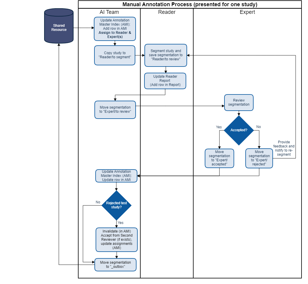
Figure 5: Manual segmentation procedure used to obtain delineations of brain tumors (alongside additional information related to the contouring, including the time of analysis and the confidence of a reader). The delineations are approved by senior radiologists. The raters provided their confidence for all GBM sub-regions, and the bidimensional measurements as per RANO were performed by each reader for Phase 3 (Post, Te). These measures were aggregated across all readers for all MRIs, and the average, weighted average (according to YOE), median, minimum, and maximum RANO was obtained for each patient as well.

For the pre- and post-operative phase 3 cohort, we enlisted two expert radiologists (Reader 1 and Reader 2, with 20 and 18 Years Of clinical Experience, YOE), together with five experienced raters (Readers 3–7 with 6, 6, 5, 3, and 2 YOE) who were tasked to analyze the input MRI scans—during the analysis process, the readers were always presented with all available MRI sequences, therefore they can benefit from all image data captured for each patient. The readers manually delineated ET, ED, and cavity (in post-surgery MRIs), following a rigorous annotation procedure (Figure 5) which expands on the BraTS annotation process by introducing the following steps:

• We capture the readers’ confidences in the quality of their annotations.

• We incorporate a redrawing/improvement step.

• We obtain the manual bidimensional RANO measurements.

Here, the sub-regions were contoured by a single reader (Reader 3–7) and then approved subsequently by one of the expert radiologists (either Reader 1 or Reader 2), that, if necessary, highlighted the tumor components that needed to be redrawn (redrawing/improvement step). For the 40 test post-surgery patients (Phase 3 [Post, Te]) used to validate the automated bidimensional RANO measurements, the manual segmentation had to be approved by both expert radiologists (Reader 1 and Reader 2). All raters used the ITK-SNAP software (version 3.6.0), and we captured the time required to contour all tumor sub-regions by each reader. The raters provided additional information regarding their confidence for all GBM sub-regions, according to the following scale:

1. I am not confident at all (almost guessing).

2. I am not confident and require advice from a senior reader.

3. I am confident to some extent, but I would prefer to have it reviewed by a senior reader.

4. I am fully confident.

Finally, bidimensional measurements as per RANO were performed by each reader for Phase 3 (Post, Te). These measures were additionally aggregated across all readers for all MRIs, and the average, weighted average (according to YOE), median, minimum, and maximum RANO was obtained for each patient.

2.3 Segmenting brain tumors from multi-modal MRI using deep learning

Our segmentation algorithm operates on the co-registered native T1, post-contrast T1, T2-weighted and FLAIR MRI sequences, all in the axial orientation (Figure 6). The approach is split into three pivotal steps: (i) pre-processing, including re-orientation and re-sampling of sequences, together with skull stripping (brain extraction), (ii) brain tumor segmentation using an ensemble of deep learning models, and (iii) post-processing of the resulting segmentation map.

Figure 6: A schematic view of our processing pipeline. In light orange, we render the pre-processing steps performed before feeding the data into the ensemble model, in green—an additional pre-processing created using an nnU-Net engine for each model within our ensemble (including data augmentation and z-scoring), together with the segmentation step and post-processing, in red—calculation of bidimensional and volumetric tumor metrics, finally in gray—generating the final report, e.g., in a DICOM-RT format.

2.3.1 Pre-processing

In the pre-processing step, we use HD-BET [Isensee et al., 2019] for brain extraction in each sequence separately (see the examples in Figure 7). In parallel, the sequence with the smallest voxel size $S_{R}$ is determined and re-oriented to the Right, Anterior, Superior (RAS) coordinate system. The brain probability maps, alongside all other sequences $S$ are later linearly re-sampled to $S_{R}$. Finally, the brain probability maps are binarized, and skull stripping is performed in all sequences.

Figure 7: Two examples of post-operative MRIs from Phase 3 (Post, Tr) before and after brain extraction (skull stripping). Skull stripping is one of the pre-processing steps in the analysis pipeline. P1 and P2 denote patient 1 and patient 2, respectively.

2.3.2 Ensemble of the confidence-aware nnU-Nets

A single ensemble of five confidence-aware nnU-Nets (see the detailed model architecture in the Supplementary Material) trained over different training sets is used to process both pre- and post-operative MRIs, and to automatically detect ET, ED, and cavity areas. It receives, as inputs, pre-processed native T1, post-contrast T1, T2-weighted and FLAIR sequences and performs z-score normalization, hence each sequence is normalized independently through extracting its mean intensity value and dividing by standard deviation. The base deep models are assembled by averaging softmax probabilities. During the prediction, the full MRIs with up to four modalities are inputted.

The models are trained with the loss function $\mathcal{L}$, being the averaged cross-entropy and soft DICE, averaged across all target classes ET, ED, and Cavity:

$$\mathcal{L}=\frac{\mathcal{L}({\rm ET})+\mathcal{L}({\rm ED})+\mathcal{L}({\rm Cavity})}{3}.$$ (1)

The soft DICE loss becomes

$$\mathcal{L}_{\rm DICE}=1-\frac{2\left|P\cap GT\right|}{\left|P\right|^{2}+\left|GT\right|^{2}},$$ (2)

where $P$ and $GT$ indicate the predicted and ground-truth (GT) segmentation masks. To exploit the reader’s confidence available for Phase 3 (Pre) and Phase 3 (Post, Tr) training MRIs, the loss was modified:

$$\mathcal{L}^{\prime}=\frac{\mathcal{L}^{\prime}({\rm ET})+\mathcal{L}^{\prime}({\rm ED})+\mathcal{L}^{\prime}({\rm Cavity})}{3},$$ (3)

where $\mathcal{L}^{\prime}(\mathcal{C})=\mathcal{L}(\mathcal{C})\cdot\alpha(\mathcal{C})$, $\mathcal{C}\in\{{\rm ET},{\rm ED},{\rm Cavity}\}$, and $\alpha$ denotes the multiplier related to the corresponding level of confidence. The following mapping is exploited: 0.5 for the confidence of 1 (i.e., “I am not confident at all…”), 0.75 for 2, 1.25 for 3, and 1.5 for 4—the higher the confidence of the GT segmentation is, the larger impact on the loss it has. The mapping was non-linear to better separate acceptable (confidence 3 and 4) and non-acceptable (confidence 1 and 2) cases. For the MRIs (or specific sub-region types) without reported raters’ confidences, $\alpha({\rm ET})=\alpha({\rm ED})=\alpha({\rm Cavity})=1$ is used during training.

2.3.3 Post-processing

Most MRIs used in our study were performed more than 5 days after surgery. As a result, the MRI acquisition does not avoid the contrast enhancement associated with the surgical intervention. Therefore, since enhancing tumor area are typically located within invaded tissues, in order to avoid false positives (FPs) that may arise from hyper-intense regions in post-contrast T1 along the surgical cavity [Lescher et al., 2014], as a post-processing step, we remove all detected ET voxels that were not neighboring to ED (in 3D)—an example segmentation before and after the suggested post-processing is rendered in Figure 8.

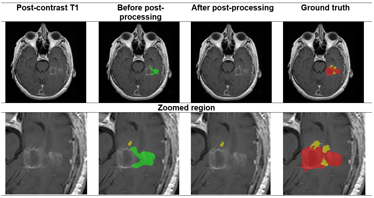
Figure 8: The proposed post-processing routine allows for pruning false positive ET sub-regions. Green shows the predicted ET region, yellow shows predicted ED, whereas red shows the surgical cavity in the ground truth. A part of the image is zoomed in the second row.

2.3.4 Splitting training data into stratified folds and evaluating the model

All 933 training MRIs were split into five non-overlapping folds used for training base models in our segmentation ensemble. To maintain the original distribution of ET and ED volumes within all subsets, each training set (BraTS 2020 [Tr], Phase 3 [Pre], and Phase 3 [Post, Tr]) was split into five stratified folds, according to the ET and ED volume distributions (Figure 2). The corresponding folds from each set were combined (i.e., Fold 1 from BraTS 2020 [Tr], Phase 3 [Pre], and Phase 3 [Post, Tr], and so forth). Each base model in an ensemble is trained for 1000 epochs using stochastic gradient descent with Nesterov momentum ($\mu=0.99$) on a training set composed of four different folds, with one fold kept aside and acting as the validation set. The batch included two patches of size 208×238×196, and 250 batches were processed within an epoch. Training-time data augmentation encompassed random patch scaling within (0.7, 1.4), random rotation, random gamma correction within (0.7, 1.5), and random mirroring [Nalepa et al., 2019a].

2.3.5 Automated bidimensional measurements

We introduce a fully automatic algorithm for calculating bidimensional measurements in post-contrast T1 sequences, strictly following the current RANO criteria [Ellingson et al., 2017]. For each detected ET region in the input 3D volume, the algorithm exhaustively searches for the longest segment (major diameter) over all slices, and then for the corresponding longest perpendicular diameter, with the tolerance of 5 degrees inclusive. Such segments are valid if they (i) are fully inscribed in ET, and (ii) are both at least 10 mm long (otherwise, the lesion is not measurable). Finally, the product of the perpendicular diameters is calculated. If there are more measurable ET regions, the sum of up to five largest products is returned. We refer to this algorithm as Automated RANO (Diameters). In addition, we introduce an alternative and more robust version of the automated two-dimensional RANO (Automated RANO [Product]), that exhaustively optimizes the product of diameters instead of the maximum diameter. We found this approach to be less sensitive to small alterations in the contour of the lesions.

2.3.6 Quantitative and statistical analysis

To evaluate the manual and automated segmentation, we computed the DICE coefficient, the Jaccard’s index (also referred to as the Intersection over Union, IoU), sensitivity and specificity. For those parameters, the larger value obtained the better, with 1.0 denoting a perfect score. The DICE coefficient is calculated as:

$${\rm DICE(P,GT)}=\frac{2\cdot\left|{\rm P}\cap{\rm GT}\right|}{\left|{\rm P}\right|+\left|{\rm GT}\right|}=\frac{\rm 2\cdot TP}{\rm 2\cdot TP+FP+FN},$$ (4)

whereas for IoU we have:

$${\rm IoU(P,GT)}=\frac{\left|{\rm P}\cap{\rm GT}\right|}{\left|{\rm P}\cup{\rm GT}\right|}=\frac{\rm TP}{\rm TP+FP+FN},$$ (5)

where P and GT are two segmentations (predicted and ground truth), and TP, FP, and FN are the numbers of true positives, false positives, and false negatives. Both DICE and IoU are the overlap metrics, but can notice that IoU penalizes single instances of wrong segmentation more than DICE, therefore IoU tends to quantify the “worst” case average performance of the segmentation algorithm.

In addition, the 95^th percentile of Hausdorff distance (H95; the smaller, the better), which quantifies the contours’ similarity, was also calculated [Bakas et al., 2018]. Since the shape of the ET contours may easily affect the RANO calculation, e.g., jagged contours could result in over-pessimistic bidimensional measurements, investigating both overlap measures (e.g., DICE/IoU) together with H95 is pivotal to thoroughly quantify the algorithm’s capabilities, as it should simultaneously obtain maximum overlap metrics and maintain minimum distance between the automatic and manual contours. The inter-rater and algorithm-rater agreement for bidimensional and volume measurements was evaluated using the Intraclass Correlation Coefficient (ICC) calculated on a single measurement, absolute-agreement, two-way random-effects model. The R package IRR (Inter Rater Reliability, version 0.84.1) was used for ICC, whereas GraphPad Prism 9.1.2 for calculating the Spearman’s correlation coefficient ($\rho$) and all other statistics.

2.3.7 Implementation details and code availability

The proposed deep learning pipeline was implemented in Python 3.7 with the PyTorch 1.6.0 backend. Our segmentation model is built upon an established open-sourced nnU-Net framework [Isensee et al., 2021a] available at https://github.com/MIC-DKFZ/nnUNet, whereas for brain extraction we utilize the HD-BET software [Isensee et al., 2019] available at https://github.com/MIC-DKFZ/HD-BET. To ensure full reproducibility of the deep learning segmentation algorithm, we present the details of the deep model architecture in the Supplementary Material.

3 Results

This section gathers the results of our experimental study. We focus on the pivotal aspects of the pipeline, including the quality of tumor segmentation (Section 3.1), RANO measurements (Section 3.2), correlations between RANO and volumetric measurements (Section 3.3), and its processing time (Section 3.4).

3.1 Segmentation of brain tumors

The performance of our segmentation algorithm was evaluated for a pre-surgery set using BraTS 2020 (V) (which included 125 patients). For computing the performance matrix in the post-surgery setting, for ET we used 32 patients with existing ground-truth ET regions from Phase 3 (Post, Te), whereas for evaluating ED, this was 39 patients with existing ground-truth ED regions.

For pre-operative patients, mean DICE for ET was 0.744 (95% CI: 0.690–0.799) with median DICE of 0.871 (25% percentile–75% percentile, 25p–75p: 0.776–0.917). The corresponding mean H95 was 39.624 mm with median H95 of 2.000 mm (25p–75p: 1.000–3.399 mm). The cavity was erroneously detected in pre-operative patients: 8/125 patients (6.4%) for BraTS 2020 (V) and 10/166 patients (6.0%) for BraTS 2020 (Te), respectively. The cavity detection results are gathered in Table 3, in which we confront our model with the vanilla nnU-Nets trained on either post-operative training MRIs, or all training MRIs.

Table 3: The surgical cavity detection results obtained over pre-operative patients (any detections are false positives) for BraTS 2020 (V) and BraTS 2020 (Te) by the vanilla nnU-Net trained on post-operative training MRIs (Post) or all training MRIs, and by the proposed model. The best results are boldfaced, and the worst results are underlined.

Metric$\downarrow$	nnU-Net (Post)	nnU-Net	Proposed
BraTS 2020 (V), 125 pre-operative patients
Number of patients with detected cavity	102	8	8
Percentage of patients with detected cavity	81.60%	6.40%	6.40%
Mean vol. of detected cavity [mm3]	10468.03	5611.75	5931.38
Min. vol. of detected cavity [mm3]	1	4	6
Max. vol. of detected cavity [mm3]	70927	22576	25491
Median vol. of detected cavity [mm3]	5019	792	981
BraTS 2020 (Te), 166 pre-operative patients
Number of patients with detected cavity	128	12	10
Percentage of patients with detected cavity	77.10%	7.20%	6.00%
Mean vol. of detected cavity [mm3]	9772.15	735.17	468.1
Min. vol. of detected cavity [mm3]	2	3	34
Max. vol. of detected cavity [mm3]	85582	6904	2565
Median vol. of detected cavity [mm3]	4404	73	202

For post-operative patients, the median DICE for ET was 0.735 (25p–75p: 0.588–0.801). The mean DICE was 0.692 (95% CI: 0.628–0.757), 0.677 (0.631–0.724) and 0.691 (0.604–0.778) for ET, ED, and surgical cavity. The respective values for mean H95 were 9.221 mm (6.437–12.000 mm), 9.455 mm (7.176–11.730 mm) and 7.956 mm (5.938–9.975 mm). The mean DICE for ET was significantly larger for the data segmented with the highest confidence by the readers, 0.749 (95% CI: 0.698–0.800) for confidence level 4 compared to 0.599 (95% CI: 0.452–0.746) for the remainder (reader confidence level 1 to 3).

Exploiting the readers’ confidence improved the segmentation capabilities of the deep learning models, significantly outperforming the other techniques as indicated with DICE/H95 analysis. The mean and median values of all quality metrics were improved for the ET area, as well as for T2/FLAIR abnormalities (ED). Finally, detecting the surgical cavity automatically resulted in further improvements in the quality of ET delineation. The automated volumetric measurements (in mm³) for ET and the surgical cavity sub-regions were in almost perfect agreement with the ground-truth segmentations (ICC: 0.959, $p<0.001$, Figure 9a, ICC: 0.960, $p<0.001$, Figure 9c, respectively), whereas for ED the agreement was ICC: 0.703 ($p<0.703$; Figure 9b).

Figure 9: Bland-Altman plots for a) ET, b) ED, and c) cavity volumes extracted manually (GT) and the algorithm for all post-operative MRIs showing that the model is in almost perfect agreement for ET and surgical cavity.

Table 4: The results obtained in post-surgery setting, with all MRI sequences included, as well as if T2-weighted or FLAIR are voluntarily omitted. The best results are boldfaced, whereas the worst—underlined.

		Without	Without			Without	Without			Without	Without
Metric$\downarrow$	All MRI	T2w	FLAIR		All MRI	T2w	FLAIR		All MRI	T2w	FLAIR
DICE
	ET				ED				Cavity
25p	0.588	0.617	0.099		0.615	0.529	0.156		0.596	0.227	0.488
Median	0.735	0.741	0.674		0.708	0.674	0.250		0.774	0.680	0.786
75p	0.801	0.795	0.790		0.769	0.751	0.470		0.908	0.877	0.883
Mean	0.692	0.684	0.521		0.677	0.654	0.302		0.691	0.570	0.641
Lower 95% CI	0.628	0.613	0.401		0.631	0.606	0.228		0.604	0.463	0.542
Upper 95% CI	0.757	0.755	0.641		0.724	0.702	0.375		0.778	0.678	0.741
IoU
	ET				ED				Cavity
25p	0.416	0.447	0.062		0.444	0.360	0.085		0.425	0.130	0.323
Median	0.581	0.588	0.509		0.548	0.509	0.143		0.631	0.517	0.648
75p	0.668	0.660	0.653		0.625	0.601	0.307		0.832	0.781	0.791
Mean	0.553	0.547	0.413		0.528	0.502	0.200		0.583	0.469	0.538
Lower 95% CI	0.488	0.478	0.311		0.478	0.451	0.143		0.495	0.369	0.442
Upper 95% CI	0.617	0.617	0.515		0.578	0.554	0.258		0.671	0.569	0.633
H95
	ET				ED				Cavity
25p	3.400	3.518	4.894		5.315	4.599	15.120		3.241	4.486	3.871
Median	8.204	7.620	8.279		8.348	8.634	20.780		6.391	9.575	6.529
75p	12.610	12.330	20.700		12.120	12.340	34.250		11.150	20.010	11.870
Mean	9.221	9.532	14.060		9.455	10.010	24.960		7.956	13.560	10.650
Lower 95% CI	6.437	6.663	8.524		7.176	7.712	20.280		5.938	9.334	6.945
Upper 95% CI	12.000	12.400	19.590		11.730	12.310	29.650		9.975	17.780	14.360
Sensitivity
	ET				ED				Cavity
25p	0.626	0.643	0.081		0.628	0.543	0.085		0.491	0.133	0.348
Median	0.752	0.768	0.628		0.728	0.705	0.491		0.756	0.572	0.746
75p	0.872	0.880	0.783		0.775	0.762	0.324		0.925	0.844	0.898
Mean	0.720	0.720	0.504		0.695	0.665	0.213		0.662	0.522	0.613
Lower 95% CI	0.646	0.644	0.381		0.651	0.613	0.148		0.563	0.410	0.506
Upper 95% CI	0.794	0.796	0.627		0.738	0.717	0.277		0.762	0.633	0.719
Specificity
	ET				ED				Cavity
25p	0.9995	0.9992	0.9997		0.9992	0.9991	0.9999		0.9996	0.9997	0.9995
Median	0.9998	0.9998	0.9998		0.9996	0.9996	1.0000		0.9998	0.9999	0.9998
75p	0.9999	0.9999	1.0000		0.9998	0.9998	1.0000		0.9999	1.0000	1.0000
Mean	0.9995	0.9994	0.9997		0.9992	0.9991	0.9999		0.9997	0.9998	0.9997
Lower 95% CI	0.9993	0.9991	0.9995		0.9986	0.9986	0.9999		0.9995	0.9997	0.9995
Upper 95% CI	0.9998	0.9997	0.9999		0.9997	0.9997	1.0000		0.9998	0.9999	0.9998

The algorithm is trained and originally designed to work with a set of four MRI sequences: T1 pre/post contrast, T2-weighted and FLAIR. To check the robustness of our segmentation technique in the case of missing sequences, we voluntarily omitted either T2-weighted or FLAIR during the prediction process (Table 4). Here, we did not remove native T1 and post-contrast T1, as those are pivotal in visualizing and quantifying ET [Ellingson et al., 2014]. After removing T2-weighted, the mean (median) DICE scores changed by ↓0.009 (↑0.006) for ET, ↓0.024 (↓0.033) for ED, and ↓0.121 (↓0.094) for cavity. Omitting FLAIR resulted in changing the mean (median) DICE by ↓0.172 (↓0.061) for ET, ↓0.376 (↓0.458) for ED, and ↓0.050 (↑0.012) for cavity. The differences in the overlap metrics (DICE and IoU) are statistically significant for ET and ED only in the case of removing FLAIR ($p<0.0001$, Wilcoxon matched-pairs signed rank test). Similarly, automated RANO (Diameters) and Automated RANO (Product) are statistically significantly different after removing FLAIR ($p<0.0001$), but not after removing the T2-weighted sequence. For the surgical cavity, however, the decrease in these metrics is significant if either T2-weighted or FLAIR are missing ($p<0.0001$).

Table 5: The Intraclass Correlation Coefficient (ICC) obtained for the bidimensional measurements (RANO) across all readers and aggregations of readers’ responses, as well as for Automated RANO—two algorithms, one maximizing the major and perpendicular diameters sequentially (referred as Diameters), and the other optimizing the product of the perpendicular diameters (Product). Best results in green, worse in red.

			Auto. RANO	Auto. RANO
	GT (Diam.)	GT (Prod.)	(Diameters)	(Product)
Reader 1	0.760	0.701	0.681	0.671
Reader 2	0.683	0.822	0.866	0.858
Reader 3	0.406	0.328	0.299	0.292
Reader 4	0.332	0.447	0.583	0.537
Reader 5	0.650	0.516	0.489	0.460
Reader 6	0.588	0.461	0.441	0.414
Reader 7	0.515	0.401	0.394	0.373
Average	0.688	0.628	0.657	0.617
Weighted average	0.777	0.771	0.807	0.772
Median	0.601	0.505	0.499	0.472
Minimum	0.287	0.240	0.221	0.215
Maximum	0.725	0.868	0.915	0.919
GT (Diameters)		0.935	0.852	0.843
GT (Product)			0.934	0.944
Auto. RANO (Diameters)				0.981

3.2 Inter-rater agreement for RANO bidimensional measurements

There was a significant inter-rater variability and disagreement across the human readers for the bidimensional RANO calculation in the post-surgery setting (Phase 3 [Post, Te] dataset), with ICC: 0.220–0.960 (Table 5). The agreement between the manual RANO provided by the raters and Automated RANO (Diameters) calculated over the predicted ET regions was ICC: 0.299–0.866 ($p<0.001$), whereas for Automated RANO (Product) it amounted to 0.292–0.858 ($p<0.001$). Automated RANO (Diameters) and Automated RANO (Product) were in strong agreement with the maximum values aggregated across all human raters, ICC: 0.915 ($p<0.001$) and 0.919 ($p<0.001$). Both versions of the automated RANO were consistently resulting in larger ICC with the most senior radiologists (Figure 10) compared to less-experienced readers (Table 6).

Figure 10: Bland-Altman plots for a) Automated RANO (Diameters) and b) Automated RANO (Product) (both calculated using the algorithm derived ET segmentation using all post-operative MRIs) and i) senior radiologists (Reader 1 and Reader 2), ii) the least experienced rater (Reader 7, 2 YOE), iii) the maximum RANO calculated for each patient across all the readers, iv) Automated RANO (Diameters) calculated over the GT segmentations, and v) Automated RANO (Product) calculated over the GT segmentations. Our algorithm consistently delivers the largest agreement with the senior radiologists and tends to return larger RANO as it carefully optimizes the RANO diameters.

Table 6: The Intraclass Correlation Coefficient (ICC) obtained for the bidimensional measurements (RANO) across all readers (R1–R7 in the column headers) and all aggregations of readers’ responses (Phase 3 [Post, Te] test MRIs). Best results in green, worse in red.

	R2	R3	R4	R5	R6	R7	Avg.	W avg.	Median	Min.	Max.
Reader 1	0.580	0.711	0.566	0.829	0.765	0.730	0.934	0.920	0.880	0.534	0.601
Reader 2		0.220	0.621	0.360	0.310	0.265	0.585	0.776	0.406	0.200	0.966
Reader 3			0.334	0.774	0.729	0.793	0.746	0.564	0.856	0.814	0.243
Reader 4				0.335	0.334	0.317	0.684	0.741	0.512	0.317	0.574
Reader 5					0.960	0.889	0.863	0.720	0.936	0.592	0.403
Reader 6						0.899	0.821	0.660	0.924	0.602	0.343
Reader 7							0.807	0.614	0.920	0.696	0.288
Average								0.937	0.943	0.615	0.578
Weighted avg.									0.793	0.459	0.758
Median										0.725	0.413
Minimum											0.185

3.3 Correlation between bidimensional RANO and volumetric measurements

The Spearman’s correlation coefficient $\rho$ between the RANO bidimensional values and ground-truth ET volumes calculated by the readers ranged from 0.405 (Reader 6) to 0.849 (Reader 1). For aggregated RANO values, $\rho$ was between 0.520 (minimum RANO across the raters) and 0.862 (maximum RANO across the raters), as presented in Figure 11. Automated RANO strongly correlates with the ET volume (Figure 12), $\rho$: 0.948 and 0.965 for GT (Automated RANO [Diameters] and Automated RANO [Product]), and $\rho$: 0.899 and 0.904 for our predictions (Automated RANO [Diameters] and Automated RANO [Product]).

Figure 11: Correlation between the ground-truth ET volume [mm³] and bidimensional measurements (RANO) [mm²] calculated by the readers, and by aggregating the results delivered by the raters (average, weighted average according to the years of experience, median, minimum, and maximum across all readers for each patient), for all post-operative MRIs.

Figure 12: Correlation between the ground-truth ET volume [mm³] and bidimensional measurements (RANO) [mm²] obtained using a) Automated RANO (Diameters) and b) Automated RANO (Product) over the ground-truth (GT) segmentations and delivered by the algorithm for all post-operative MRIs. The RANO calculated using the algorithms is in almost perfect correlation with the ET volume, and the strength of this correlation is significantly larger than for RANO measured by the readers.

3.4 Processing time analysis

The experiments were executed on a high-performance computer equipped with an NVIDIA Tesla V100 GPU (32 GB) and 6 Intel Xeon E5-2680 (2.50 GHz) CPUs. The average end-to-end analysis time amounted to 148 s (with Automated RANO [Diameters]) and 829 s (with Automated RANO [Product]). This time includes brain extraction (81 s on average), other pre-processing routines (13 s), brain tumor segmentation (43 s), post-processing (1 s), and Automated RANO (Diameters) and Automated RANO (Product) calculation, 8 s and 678 s, respectively. In comparison, the average manual tumor segmentation time was 33, 39, 41, 50, and 36 mins for Readers 3–7. The algorithm is therefore at least 20.3× (Automated RANO [Diameters]) and 3.6× (Automated RANO [Product]) faster than the radiologists (we did not capture the time required for reader RANO calculation, only the duration of the manual image segmentation).

4 Discussion

Evaluating response to therapies in GBM depends extensively on the longitudinal radiological assessment of MRI scans to estimate change in tumor burden. This is based on two dimensional diameter measurements of enhancing tumors as well as on the qualitative estimation of T2/FLAIR abnormalities. Given the irregular shape and heterogeneous appearance of GBM lesions, this procedure is notoriously complex to perform and subject to high intra- and inter-reader variability, which, in turn, limits our ability to detect a therapeutic benefit in clinical trials and capture early patient response or progression in clinical practice. Volumetric analysis of all the lesions has also long been recognized as a potential alternative response endpoint to bidimensional RANO assessment. Because of the prohibitively highly tedious and time-consuming process of segmenting tumor lesions manually, integration of volumetric measurement into the clinical workflow is, however, only feasible with the advent of automation.

Our deep learning model is able to segment several tumor sub-regions simultaneously, including enhancing tumor area (ET) and T2/FLAIR abnormalities (ED). It has been developed by rigorously verifying 34 deep learning architectures (for the details of the investigated deep learning models, and the experimental results obtained for each of them, see the Supplementary Material) trained and tested on a large dataset consisting of 464 post-operative training and 40 test clinical multi-modal MRIs obtained from 92 institutions and multiple scanner types around the world that were manually annotated by 7 expert readers. Expanding the training sets to include additional pre-operative (469) patients as well as exploiting the readers’ confidence brought significant improvements of the segmentation quality metrics. Detecting the surgical cavity automatically allowed the model to further improve by capturing contextual information about the tumor’s sub-regions more comprehensively. This was achieved due to low prevalence of false positive and erroneous detection of surgical cavity and by the fact that when cavity was incorrectly annotated, this corresponded to the necrotic and non-enhancing tumor core with no impact on ET, ED and RANO tumor measurements (Figure 13).

Figure 13: Incorrectly predicted cavity regions (in red) in pre-operative patients. This corresponded to the necrotic and non-enhancing tumor core (in blue, as returned by the cascaded 3D U-Nets [Kotowski et al., 2020]) and therefore did not impact the RANO calculation.

In the pre-surgery setting, the developed segmentation algorithm outperformed the recently introduced cascaded 3D U-Nets [Kotowski et al., 2020] in all segmentation quality metrics (Table 7). For post-operative patients, we also obtained high performance, comparable to the results reported by Chang et al. [2019] and showing that the segmentation algorithm can be used successfully for pre- or post-operative patients. Although we are aware that confronting the results of the algorithms over different test sets may easily be misleading, a large number of MRIs taken for investigation should compensate it and “protect” us from inferring over-optimistic conclusions with respect to the state of the art.

We tested the robustness of the algorithm by voluntarily removing one imaging sequence (T2-weighted or FLAIR) from the model inputs. Overall, contrary to FLAIR and with the exception of the surgical cavity, the quality of the sub-region segmentation (ET and ED) as well as RANO bidimensional measurements are not statistically significantly compromised if T2-weighted images are not used (Table 4). This reflects the preference of radiologists for using FLAIR for image evaluation as the nulling of the cerebrospinal fluid signal in this sequence augments the conspicuity of tumor lesions compared to T2-weighted sequences. Overall, removing T2-weighted from the input does not significantly affect ET or ED segmentation—the algorithm is sufficiently robust to be used with only native T1, post-contrast T1 and FLAIR (without T2-weighted sequences). We also evaluated the model performance early after surgery using the only patient dataset acquired within a few days after surgical intervention. Early post-operative scans are known to avoid surgically induced contrast enhancement, minimizing interpretative difficulties. While additional assessments would be beneficial in that setting, for the patient scanned 1 day after surgery the DICE and H95 value for ET (0.717, 5.99 mm) were comparable to the complete dataset (mean: 0.692, 9.221 mm, median: 0.735, 8.204 mm).

Table 7: The segmentation results obtained for BraTS 2020(V) using cascaded 3D U-Nets [Kotowski et al., 2020] (with and without exploiting the expert knowledge, as proposed by Kotowski et al. [2020]), and the models introduced in this study. The best results for each metric are bold, and the worst—underlined.

		Cascaded	Cascaded 3D	nnU-Net
Metric$\downarrow$		3D U-Nets	U-Nets with EK	(Post)	nnU-Net	Proposed
DICE	Mean	0.685	0.694	0.720	0.750	0.744
	s	0.315	0.310	0.278	0.301	0.307
	Median	0.839	0.842	0.838	0.872	0.871
	25q	0.618	0.623	0.674	0.772	0.781
	75q	0.891	0.894	0.883	0.914	0.915
H95	Mean	47.45	43.95	28.63	36.82	39.62
	s	112.71	108.93	90.68	106.06	109.85
	Median	2.83	2.83	2.24	2.00	2.00
	25q	1.41	1.41	1.73	1.00	1.00
	75q	14.01	11.53	9.52	3.30	3.40
Sensitivity	Mean	0.682	0.690	0.717	0.756	0.752
	s	0.328	0.324	0.307	0.319	0.325
	Median	0.825	0.827	0.848	0.886	0.890
	25q	0.595	0.600	0.615	0.756	0.758
	75q	0.902	0.905	0.928	0.951	0.947
Specificity	Mean	0.9997	0.9997	0.9997	0.9998	0.9998
	s	0.0004	0.0004	0.0004	0.0004	0.0004
	Median	0.9998	0.9998	0.9999	0.9999	0.9999
	25q	0.9996	0.9996	0.9995	0.9996	0.9996
	75q	1.0000	1.0000	1.0000	1.0000	1.0000

The deep learning tumor segmentation was subsequently used to automatically obtain the tumor volumes and the bidimensional tumor measurements according to the Response Assessment in Neuro-Oncology (RANO) criteria. The results were then compared with measurements from experts. The tumor volumes extracted automatically were in almost perfect agreement with the values obtained by the readers (Figure 9). For RANO, there was a significant disagreement across human raters which reflects the difficulty for radiologists to perform GBM tumor burden measurements, particularly in post-surgery settings, and the benefit that automation might bring. There were several indications that the deep learning model is more reliable and accurate than humans:

• The algorithms had the highest agreements with the most expert radiologists (Figure 10).

• The pipeline returned higher bidimensional measurement than those reported by most human readers because the algorithm carefully finds the maximal enhancing tumor diameters (or their product) which cannot be done as reliably by a radiologist in a manual process (Figure 14).

• The automated RANO correlated better with ground truth enhancing tumor volume than the RANO done by the readers (Figure 11).

It is worth mentioning that optimizing the product of diameters instead of the maximum diameter was more effective at compensating for eventual errors in tumor segmentation and therefore provided more robust RANO measurement.

Figure 14: Qualitative and quantitative analysis can reveal important aspects concerning the behavior and abilities of the suggested pipeline—an example axial post-contrast T1 image and manual segmentation (green—ET, yellow—ED, red—surgical cavity). Below, the RANO bidimensional measurements for the two most experienced readers compared with Automated RANO (Diameters) and Automated RANO (Product) obtained from either the ground-truth or the algorithm’s segmentation. Manual calculation of RANO is subjective, difficult to reproduce and may easily lead to high inter-rater disagreement—the proposed algorithm offers full reproducibility and a more accurate optimization of the product diameters leading to a stronger correlation with the ET volume.

Figure 15: The examples of tumors with very different volume but with almost identical bidimensional RANO measurements, showing that in some cases, relying on 2D measurement can be misleading.

The high correlation observed between RANO and tumor volume supports the concept of using bidimensional measurement for evaluating tumor burden in GBM patients. Nevertheless, while routinely applied, there are clearly limitations inherent to this approach as highlighted, for instance, by two patients in our dataset which have very similar RANOs (Patient A: 1071.45 mm², Patient B: 1137.73 mm²) but very different tumor volumes (Patient A: 8502.33 mm³, Patient B: 66287.65 mm³). As this example shows, analyzing a 2D MRI slice is not always sufficient to accurately quantify tumor burden (Figure 15). Volumetric tumor segmentation, which requires automation for its integration into the clinical workflow, is also a necessary initial step toward more advanced image analysis that can be used to identify novel biomarkers—this includes intensity-related features, 2D and 3D shape characteristics, texture analysis of the tumor tissue [Nalepa et al., 2014], as well as other radiomic parameters [Ayadi et al., 2019] that can be used to build predictive models in diagnosis, prognosis and therapeutic response [Chaddad et al., 2019, Park et al., 2020, Suter et al., 2020].

5 Conclusions and Future Work

For patients with glioblastoma, the evaluation of tumor burden and response to therapy is based on the bidimensional measurement of the T1 contrast enhancing tumor area and the qualitative evaluation of abnormalities on T2/FLAIR MRI scans. As gliomas are often very heterogeneous in appearance and shape, this assessment is complex to perform and associated with high variability, particularly in the post-surgery setting. In this work, we approached this issue and introduced an easy to use, built upon and expanding the recent advances in the machine learning field, and thoroughly validated pipeline that automatically segments pre- and post-operative MRIs from GBM patients and delineates tumor sub-regions, including contrast enhancing area, T2/FLAIR hyperintensities and surgical cavity. The entire process, with volumetric and RANO calculations, is executed in a fraction of time needed by humans with performance matching or exceeding radiologists. The algorithm’s potential for improving and simplifying radiological assessment of glioma patients opens the door to its deployment in clinical trials—as shown in our experimental study performed over a very large number of patients—and its integration into the clinical workflow. The automatic measurements were reliable, fast and in statistically significant agreement with the most experienced radiologists. Finally, we introduced a rigorous manual delineation process that was followed by radiologists to provide ground-truth segmentations, together with additional information related to their confidence and analysis time.

The results reported in this paper constitute an interesting departure point for further research. The follow-up steps for our segmentation algorithm would be to evaluate its robustness for longitudinal assessment and its ability to adequately identify disease progression or response during the course of a number of drug treatments. Additionally, it would be interesting to compare its performance with the top-performing techniques from BraTS 2021 once they are published. Having a comprehensive and objective comparative study of the best segmentation techniques in the literature would be an important step toward building robust and certified AI-powered tools that could be utilized in clinical practice. Since gathering more clinical MRI data with the corresponding ground-truth data is extremely costly, training the algorithms in the federated learning approach bloomed as an exciting opportunity as well, as it could help us train the deep learning models over massively large training samples without the necessity of sharing them across institutions [Sheller et al., 2020]. Finally, the improvement of our deep learning pipeline might also be possible by evaluating the image features associated with poorer performance (e.g., for low-quality or deformed MRI scans), and building data augmentation routines that focus more specifically on these characteristics [Nalepa et al., 2019a].

References

- Abbas et al. [2021] Abbas, H.K., Fatah, N.A., Mohamad, H.J., Alzuky, A.A., 2021. Brain tumor classification using texture feature extraction. Journal of Physics: Conference Series 1892, 012012.
- Aboelenein et al. [2020] Aboelenein, N.M., Songhao, P., Koubaa, A., Noor, A., Afifi, A., 2020. HTTU-Net: Hybrid two track U-Net for automatic brain tumor segmentation. IEEE Access 8, 101406–101415.
- Al-Rahlawee and Rahebi [2021] Al-Rahlawee, A.T.H., Rahebi, J., 2021. Multilevel thresholding of images with improved Otsu thresholding by black widow optimization algorithm. Multimedia Tools and Applications 80, 28217–28243.
- Aljabar et al. [2009] Aljabar, P., Heckemann, R., Hammers, A., Hajnal, J., Rueckert, D., 2009. Multi-atlas based segmentation of brain images: Atlas selection and its effect on accuracy. NeuroImage 46, 726–738.
- Audelan and Delingette [2021] Audelan, B., Delingette, H., 2021. Unsupervised quality control of segmentations based on a smoothness and intensity probabilistic model. Medical Image Analysis 68, 101895.
- Ayadi et al. [2019] Ayadi, W., Elhamzi, W., Charfi, I., Atri, M., 2019. A hybrid feature extraction approach for brain MRI classification based on bag-of-words. Biomedical Signal Processing and Control 48, 144–152.
- Baid et al. [2021] Baid, U., Ghodasara, S., Bilello, M., Mohan, S., et al., 2021. The RSNA-ASNR-MICCAI BraTS 2021 Benchmark on Brain Tumor Segmentation and Radiogenomic Classification. arXiv:2107.02314.
- Bakas et al. [2017a] Bakas, S., Akbari, H., Sotiras, A., Bilello, M., Rozycki, M., Kirby, J., Freymann, J., Farahani, K., Davatzikos, C., 2017a. Advancing the cancer genome atlas glioma MRI collections with expert segmentation labels and radiomic features. Nature Scientific data 4, 1–13. doi:10.1038/sdata.2017.117.
- Bakas et al. [2017b] Bakas, S., Akbari, H., Sotiras, A., Bilello, M., Rozycki, M., Kirby, J.S., Freymann, J.B., Farahani, K., Davatzikos, C., 2017b. Segmentation labels and radiomic features for the pre-operative scans of the TCGA-GBM collection. The Cancer Imaging Archive. https://doi.org/10.7937/K9/TCIA.2017.KLXWJJ1Q.
- Bakas et al. [2017c] Bakas, S., Akbari, H., Sotiras, A., Bilello, M., Rozycki, M., Kirby, J.S., Freymann, J.B., Farahani, K., Davatzikos, C., 2017c. Segmentation labels and radiomic features for the pre-operative scans of the TCGA-LGG collection. The Cancer Imaging Archive. https://doi.org/10.7937/K9/TCIA.2017.GJQ7R0EF.
- Bakas et al. [2018] Bakas, S., Reyes, M., Jakab, A., Bauer, S., Rempfler, M., Crimi, A., Shinohara, R.T., Berger, C., Ha, S.M., Rozycki, M., Prastawa, M., Alberts, E., Lipková, J., Freymann, J.B., Kirby, J.S., Bilello, M., Fathallah-Shaykh, H.M., Wiest, R., Kirschke, J., Wiestler, B., Colen, R.R., Kotrotsou, A., LaMontagne, P., Marcus, D.S., Milchenko, M., Nazeri, A., Weber, M., Mahajan, A., Baid, U., et al., 2018. Identifying the best machine learning algorithms for brain tumor segmentation, progression assessment, and overall survival prediction in the BRATS challenge. CoRR abs/1811.02629. URL: http://arxiv.org/abs/1811.02629, arXiv:1811.02629.
- Barzegar and Jamzad [2020] Barzegar, Z., Jamzad, M., 2020. A reliable ensemble-based classification framework for glioma brain tumor segmentation. Signal, Image and Video Processing 14, 1591–1599.
- Bauer et al. [2010] Bauer, S., Seiler, C., Bardyn, T., Buechler, P., Reyes, M., 2010. Atlas-based segmentation of brain tumor images using a Markov Random Field-based tumor growth model and non-rigid registration, in: Proc. IEEE EMB, pp. 4080–4083.
- Ben naceur et al. [2020] Ben naceur, M., Akil, M., Saouli, R., Kachouri, R., 2020. Fully automatic brain tumor segmentation with deep learning-based selective attention using overlapping patches and multi-class weighted cross-entropy. Medical Image Analysis 63, 101692.
- Ben Rabeh et al. [2017] Ben Rabeh, A., Benzarti, F., Amiri, H., 2017. Segmentation of brain MRI using active contour model. International Journal of Imaging Systems and Technology 27, 3–11.
- Cahall et al. [2019] Cahall, D.E., Rasool, G., Bouaynaya, N.C., Fathallah-Shaykh, H.M., 2019. Inception modules enhance brain tumor segmentation. Frontiers in Computational Neuroscience 13, 44.
- Chaddad et al. [2019] Chaddad, A., Kucharczyk, M.J., Daniel, P., Sabri, S., Jean-Claude, B.J., Niazi, T., Abdulkarim, B., 2019. Radiomics in glioblastoma: Current status and challenges facing clinical implementation. Front. in Oncology 9, 374.
- Chang et al. [2019] Chang, K., Beers, A.L., Bai, H.X., Brown, J.M., Ly, K.I., Li, X., Senders, J.T., Kavouridis, V.K., Boaro, A., Su, C., Bi, W.L., Rapalino, O., Liao, W., Shen, Q., Zhou, H., Xiao, B., Wang, Y., Zhang, P.J., Pinho, M.C., Wen, P.Y., Batchelor, T.T., Boxerman, J.L., Arnaout, O., Rosen, B.R., Gerstner, E.R., Yang, L., Huang, R.Y., Kalpathy-Cramer, J., 2019. Automatic assessment of glioma burden: a deep learning algorithm for fully automated volumetric and bidimensional measurement. Neuro-Oncology 21, 1412–1422.
- Chen et al. [2018] Chen, C.C., Juan, H.H., Tsai, M.Y., Lu, H.H.S., 2018. Unsupervised learning and pattern recognition of biological data structures with density functional theory and machine learning. Scientific Reports 8, 557.
- Chinot et al. [2014] Chinot, O.L., Wick, W., Mason, W., Henriksson, R., Saran, F., Nishikawa, R., Carpentier, A.F., Hoang-Xuan, K., Kavan, P., Cernea, D., Brandes, A.A., Hilton, M., Abrey, L., Cloughesy, T., 2014. Bevacizumab plus Radiotherapy–Temozolomide for Newly Diagnosed Glioblastoma. New England Journal of Medicine 370, 709–722.
- Chow et al. [2014] Chow, D., Qi, J., Guo, X., Miloushev, V., Iwamoto, F., Bruce, J., Lassman, A., Schwartz, L., Lignelli, A., Zhao, B., Filippi, C., 2014. Semiautomated volumetric measurement on postcontrast MR imaging for analysis of recurrent and residual disease in glioblastoma multiforme. American Journal of Neuroradiology 35, 498–503.
- Crowe et al. [2017] Crowe, E.M., Alderson, W., Rossiter, J., Kent, C., 2017. Expertise affects inter-observer agreement at peripheral locations within a brain tumor. Frontiers in Psychology 8, 1628.
- Egger et al. [2013] Egger, J., Kapur, T., Fedorov, A., Pieper, S., Miller, J.V., Veeraraghavan, H., Freisleben, B., Golby, A.J., Nimsky, C., Kikinis, R., 2013. GBM Volumetry using the 3D Slicer Medical Image Computing Platform. Scientific Reports 3, 1364.
- Ellingson et al. [2014] Ellingson, B.M., Bendszus, M., Sorensen, A.G., Pope, W.B., 2014. Emerging techniques and technologies in brain tumor imaging. Neuro-Oncology 16.
- Ellingson et al. [2017] Ellingson, B.M., Wen, P.Y., Cloughesy, T.F., 2017. Modified criteria for radiographic response assessment in glioblastoma clinical trials. Neurotherapeutics 14, 307–320.
- Essadike et al. [2018] Essadike, A., Ouabida, E., Bouzid, A., 2018. Brain tumor segmentation with Vander Lugt correlator based active contour. Computer Methods and Programs in Biomedicine 160, 103–117.
- Habib et al. [2021] Habib, H., Amin, R., Ahmed, B., Hannan, A., 2021. Hybrid algorithms for brain tumor segmentation, classification and feature extraction. Journal of Ambient Intelligence and Humanized Computing .
- Haller et al. [2013] Haller, S., Kövari, E., Herrmann, F.R., Cuvinciuc, V., Tomm, A.M., Zulian, G.B., Lovblad, K.O., Giannakopoulos, P., Bouras, C., 2013. Do brain T2/FLAIR white matter hyperintensities correspond to myelin loss in normal aging? a radiologic-neuropathologic correlation study. Acta Neuropathologica Communications 1, 14.
- Hu et al. [2021] Hu, H.X., Mao, W.J., Lin, Z.Z., Hu, Q., Zhang, Y., 2021. Multimodal brain tumor segmentation based on an intelligent UNET-LSTM algorithm in smart hospitals. ACM Transactions on Internet Technologies 21.
- Ilhan and Ilhan [2017] Ilhan, U., Ilhan, A., 2017. Brain tumor segmentation based on a new threshold approach. Procedia Computer Science 120, 580–587.
- Isensee et al. [2021a] Isensee, F., Jaeger, P.F., Kohl, S.A.A., Petersen, J., Maier-Hein, K.H., 2021a. nnU-Net: a self-configuring method for deep learning-based biomedical image segmentation. Nature Methods 18, 203–211.
- Isensee et al. [2021b] Isensee, F., Jäger, P.F., Full, P.M., Vollmuth, P., Maier-Hein, K.H., 2021b. nnU-Net for brain tumor segmentation, in: Crimi, A., Bakas, S. (Eds.), Brainlesion: Glioma, Multiple Sclerosis, Stroke and Traumatic Brain Injuries, Springer International Publishing, Cham. pp. 118–132.
- Isensee et al. [2019] Isensee, F., Schell, M., Pflueger, I., Brugnara, G., Bonekamp, D., Neuberger, U., Wick, A., Schlemmer, H.P., Heiland, S., Wick, W., Bendszus, M., Maier-Hein, K.H., Kickingereder, P., 2019. Automated brain extraction of multisequence MRI using artificial neural networks. Human Brain Mapping 40, 4952–4964.
- Kadry et al. [2021] Kadry, S., Rajinikanth, V., Raja, N.S.M., Jude Hemanth, D., Hannon, N.M.S., Raj, A.N.J., 2021. Evaluation of brain tumor using brain MRI with modified-moth-flame algorithm and Kapur’s thresholding: a study. Evolutionary Intelligence 14, 1053–1063.
- Kirtania et al. [2020] Kirtania, R., Mitra, S., Shankar, B.U., 2020. A novel adaptive k-NN classifier for handling imbalance: Application to brain MRI. Intelligent Data Analysis 24, 909–924. 4.
- Kotowski et al. [2020] Kotowski, K., Adamski, S., Malara, W., Machura, B., Zarudzki, L., Nalepa, J., 2020. Segmenting brain tumors from MRI using cascaded 3D U-Nets, in: Crimi, A., Bakas, S. (Eds.), Brainlesion: Glioma, Multiple Sclerosis, Stroke and Traumatic Brain Injuries - 6th Int. Workshop, BrainLes 2020, Springer. pp. 265–277.
- Lefkovits et al. [2016] Lefkovits, L., Lefkovits, S., Szilágyi, L., 2016. Brain tumor segmentation with optimized random forest, in: Crimi, A., Menze, B., Maier, O., Reyes, M., Winzeck, S., Handels, H. (Eds.), Brainlesion: Glioma, Multiple Sclerosis, Stroke and Traumatic Brain Injuries, Springer International Publishing, Cham. pp. 88–99.
- Lescher et al. [2014] Lescher, S., Schniewindt, S., Jurcoane, A., Senft, C., Hattingen, E., 2014. Time window for postoperative reactive enhancement after resection of brain tumors: less than 72 hours. Neurosurgical Focus FOC 37, E3.
- Liu et al. [2014] Liu, J., Li, M., Wang, J., Wu, F., Liu, T., Pan, Y., 2014. A survey of MRI-based brain tumor segmentation methods. Tsinghua Science and Technology 19, 578–595.
- Lorenzo et al. [2019] Lorenzo, P.R., Marcinkiewicz, M., Nalepa, J., 2019. Multi-modal U-Nets with boundary loss and pre-training for brain tumor segmentation, in: Crimi, A., Bakas, S. (Eds.), Brainlesion: Glioma, Multiple Sclerosis, Stroke and Traumatic Brain Injuries - 5th International Workshop, BrainLes 2019, Springer. pp. 135–147.
- Lorenzo et al. [2017] Lorenzo, P.R., Nalepa, J., Kawulok, M., Ramos, L.S., Pastor, J.R., 2017. Particle swarm optimization for hyper-parameter selection in deep neural networks, in: Proc. GECCO, pp. 481–488.
- Meier et al. [2017] Meier, R., Porz, N., Knecht, U., Loosli, T., Schucht, P., Beck, J., Slotboom, J., Wiest, R., Reyes, M., 2017. Automatic estimation of extent of resection and residual tumor volume of patients with glioblastoma. Journal of Neurosurgery JNS 127, 798 – 806.
- Meng et al. [2017] Meng, X., Gu, W., Chen, Y., Zhang, J., 2017. Brain MR image segmentation based on an improved active contour model. PLOS ONE 12, 1–28.
- Menze et al. [2015] Menze, B.H., et al., 2015. The multimodal brain tumor image segmentation benchmark (BRATS). IEEE Transactions on Medical Imaging 34, 1993–2024.
- Mishra and Deepthi [2021] Mishra, S.K., Deepthi, V.H., 2021. Brain image classification by the combination of different wavelet transforms and support vector machine classification. Journal of Ambient Intelligence and Humanized Computing 12, 6741–6749.
- Mohamed et al. [2006] Mohamed, A., Zacharaki, E.I., Shen, D., Davatzikos, C., 2006. Deformable registration of brain tumor images via a statistical model of tumor-induced deformation. Medical Image Analysis 10, 752–763.
- Nakhmani et al. [2014] Nakhmani, A., Kikinis, R., Tannenbaum, A., 2014. MRI brain tumor segmentation and necrosis detection using adaptive Sobolev snakes, in: Ourselin, S., Styner, M.A. (Eds.), Proc. SPIE Medical Imaging: Image Processing, International Society for Optics and Photonics. pp. 1061 – 1067.
- Nalepa and Kawulok [2019] Nalepa, J., Kawulok, M., 2019. Selecting training sets for support vector machines: a review. Artificial Intelligence Review 52, 857–900.
- Nalepa et al. [2019a] Nalepa, J., Marcinkiewicz, M., Kawulok, M., 2019a. Data augmentation for brain-tumor segmentation: A review. Frontiers in Computational Neuroscience 13, 83.
- Nalepa et al. [2019b] Nalepa, J., Mrukwa, G., Piechaczek, S., Lorenzo, P.R., Marcinkiewicz, M., Bobek-Billewicz, B., Wawrzyniak, P., Ulrych, P., Szymanek, J., Cwiek, M., Dudzik, W., Kawulok, M., Hayball, M.P., 2019b. Data augmentation via image registration, in: Proc. IEEE ICIP, pp. 4250–4254.
- Nalepa et al. [2020] Nalepa, J., Ribalta Lorenzo, P., Marcinkiewicz, M., Bobek-Billewicz, B., Wawrzyniak, P., Walczak, M., Kawulok, M., Dudzik, W., Kotowski, K., Burda, I., Machura, B., Mrukwa, G., Ulrych, P., Hayball, M.P., 2020. Fully-automated deep learning-powered system for DCE-MRI analysis of brain tumors. Artificial Intelligence in Medicine 102, 101769.
- Nalepa et al. [2014] Nalepa, J., Szymanek, J., Hayball, M.P., Brown, S.J., Ganeshan, B., Miles, K., 2014. Texture analysis for identifying heterogeneity in medical images, in: Chmielewski, L.J., Kozera, R., Shin, B.S., Wojciechowski, K. (Eds.), Computer Vision and Graphics, Springer International Publishing, Cham. pp. 446–453.
- Naser and Deen [2020] Naser, M.A., Deen, M.J., 2020. Brain tumor segmentation and grading of lower-grade glioma using deep learning in MRI images. Computers in Biology and Medicine 121, 103758.
- Park et al. [2020] Park, J.E., Kim, H.S., Jo, Y., Yoo, R.E., Choi, S.H., Nam, S.J., Kim, J.H., 2020. Radiomics prognostication model in glioblastoma using diffusion- and perfusion-weighted MRI. Scientific Reports 10, 4250.
- Park et al. [2014] Park, M.T.M., Pipitone, J., Baer, L.H., Winterburn, J.L., Shah, Y., Chavez, S., Schira, M.M., Lobaugh, N.J., Lerch, J.P., Voineskos, A.N., Chakravarty, M.M., 2014. Derivation of high-resolution MRI atlases of the human cerebellum at 3T and segmentation using multiple automatically generated templates. NeuroImage 95, 217–231.
- Pei et al. [2020] Pei, L., Vidyaratne, L., Rahman, M.M., Iftekharuddin, K.M., 2020. Context aware deep learning for brain tumor segmentation, subtype classification, and survival prediction using radiology images. Scientific Reports 10, 19726.
- Peng et al. [2021] Peng, J., Kim, D.D., Patel, J.B., Zeng, X., Huang, J., Chang, K., Xun, X., Zhang, C., Sollee, J., Wu, J., Dalal, D.J., Feng, X., Zhou, H., Zhu, C., Zou, B., Jin, K., Wen, P.Y., Boxerman, J.L., Warren, K.E., Poussaint, T.Y., States, L.J., Kalpathy-Cramer, J., Yang, L., Huang, R.Y., Bai, H.X., 2021. Deep learning-based automatic tumor burden assessment of pediatric high-grade gliomas, medulloblastomas, and other leptomeningeal seeding tumors. Neuro-Oncology .
- Poernama et al. [2019] Poernama, A.I., Soesanti, I., Wahyunggoro, O., 2019. Feature extraction and feature selection methods in classification of brain MRI images: A review, in: Proc. IEEE IBITeC, pp. 58–63.
- Rohlfing et al. [2010] Rohlfing, T., Zahr, N.M., Sullivan, E.V., Pfefferbaum, A., 2010. The SRI24 multichannel atlas of normal adult human brain structure. Human Brain Mapping 31, 798–819.
- Ronneberger et al. [2015] Ronneberger, O., Fischer, P., Brox, T., 2015. U-Net: Convolutional networks for biomedical image segmentation, in: Navab, N., Hornegger, J., Wells, W.M., Frangi, A.F. (Eds.), Medical Image Computing and Computer-Assisted Intervention, Springer International Publishing, Cham. pp. 234–241.
- Sagberg et al. [2019] Sagberg, L.M., Iversen, D.H., Fyllingen, E.H., Jakola, A.S., Reinertsen, I., Solheim, O., 2019. Brain atlas for assessing the impact of tumor location on perioperative quality of life in patients with high-grade glioma: A prospective population-based cohort study. NeuroImage: Clinical 21, 101658.
- Saha et al. [2021] Saha, A., Zhang, Y.D., Satapathy, S.C., 2021. Brain tumour segmentation with a muti-pathway ResNet based UNet. Journal of Grid Computing 19, 43.
- Saleem et al. [2021] Saleem, H., Shahid, A.R., Raza, B., 2021. Visual interpretability in 3D brain tumor segmentation network. Computers in Biology and Medicine 133, 104410.
- Sasank and Venkateswarlu [2021] Sasank, V.V.S., Venkateswarlu, S., 2021. Brain tumor classification using modified kernel based softplus extreme learning machine. Multimedia Tools and Applications 80, 13513–13534.
- Seo et al. [2020] Seo, H., Badiei Khuzani, M., Vasudevan, V., Huang, C., Ren, H., Xiao, R., Jia, X., Xing, L., 2020. Machine learning techniques for biomedical image segmentation: An overview of technical aspects and introduction to state-of-art applications. Medical Physics 47, e148–e167.
- Sezer et al. [2020] Sezer, S., van Amerongen, M.J., Delye, H.H.K., ter Laan, M., 2020. Accuracy of the neurosurgeons estimation of extent of resection in glioblastoma. Acta Neurochirurgica 162, 373–378.
- Sharif et al. [2018] Sharif, M., Tanvir, U., Munir, E.U., Khan, M.A., Yasmin, M., 2018. Brain tumor segmentation and classification by improved binomial thresholding and multi-features selection. Journal of Ambient Intelligence and Humanized Computing .
- Sheller et al. [2020] Sheller, M.J., Edwards, B., Reina, G.A., Martin, J., Pati, S., Kotrotsou, A., Milchenko, M., Xu, W., Marcus, D., Colen, R.R., Bakas, S., 2020. Federated learning in medicine: facilitating multi-institutional collaborations without sharing patient data. Scientific Reports 10, 12598.
- Shorten and Khoshgoftaar [2019] Shorten, C., Khoshgoftaar, T.M., 2019. A survey on image data augmentation for deep learning. Journal of Big Data 6, 60.
- Srinivasa Reddy and Chenna Reddy [2021] Srinivasa Reddy, A., Chenna Reddy, P., 2021. MRI brain tumor segmentation and prediction using modified region growing and adaptive SVM. Soft Computing 25, 4135–4148.
- Suter et al. [2020] Suter, Y., Knecht, U., Alão, M., Valenzuela, W., Hewer, E., Schucht, P., Wiest, R., Reyes, M., 2020. Radiomics for glioblastoma survival analysis in pre-operative MRI: exploring feature robustness, class boundaries, and machine learning techniques. Cancer Imaging 20, 55.
- Tajbakhsh et al. [2020] Tajbakhsh, N., Jeyaseelan, L., Li, Q., Chiang, J.N., Wu, Z., Ding, X., 2020. Embracing imperfect datasets: A review of deep learning solutions for medical image segmentation. Medical Image Analysis 63, 101693.
- Tarasiewicz et al. [2020] Tarasiewicz, T., Kawulok, M., Nalepa, J., 2020. Lightweight U-Nets for brain tumor segmentation, in: Crimi, A., Bakas, S. (Eds.), Brainlesion: Glioma, Multiple Sclerosis, Stroke and Traumatic Brain Injuries - 6th Int. Workshop, Springer. pp. 3–14.
- Varuna Shree and Kumar [2018] Varuna Shree, N., Kumar, T.N.R., 2018. Identification and classification of brain tumor MRI images with feature extraction using DWT and probabilistic neural network. Brain Informatics 5, 23–30.
- Visser et al. [2019] Visser, M., Müller, D., van Duijn, R., Smits, M., Verburg, N., Hendriks, E., Nabuurs, R., Bot, J., Eijgelaar, R., Witte, M., van Herk, M., Barkhof, F., de Witt Hamer, P., de Munck, J., 2019. Inter-rater agreement in glioma segmentations on longitudinal MRI. NeuroImage: Clinical 22, 101727.
- Visser et al. [2020] Visser, M., Petr, J., Müller, D.M.J., Eijgelaar, R.S., Hendriks, E.J., Witte, M., Barkhof, F., van Herk, M., Mutsaerts, H.J.M.M., Vrenken, H., de Munck, J.C., De Witt Hamer, P.C., 2020. Accurate MR image registration to anatomical reference space for diffuse glioma. Frontiers in Neuroscience 14, 585.
- Wadhwa et al. [2019] Wadhwa, A., Bhardwaj, A., Singh Verma, V., 2019. A review on brain tumor segmentation of MRI images. Magnetic Resonance Imaging 61, 247–259.
- Wang et al. [2019] Wang, G., Li, W., Ourselin, S., Vercauteren, T., 2019. Automatic brain tumor segmentation based on cascaded convolutional neural networks with uncertainty estimation. Frontiers in Computational Neuroscience 13, 56.
- Wu et al. [2021] Wu, X., Bi, L., Fulham, M., Feng, D.D., Zhou, L., Kim, J., 2021. Unsupervised brain tumor segmentation using a symmetric-driven adversarial network. Neurocomputing 455, 242–254.
- Xiong et al. [2021] Xiong, S., Wu, G., Fan, X., Feng, X., Huang, Z., Cao, W., Zhou, X., Ding, S., Yu, J., Wang, L., Shi, Z., 2021. MRI-based brain tumor segmentation using FPGA-accelerated neural network. BMC Bioinformatics 22, 421.
- Yu et al. [2021] Yu, Y., Wu, X., Chen, J., Cheng, G., Zhang, X., Wan, C., Hu, J., Miao, S., Yin, Y., Wang, Z., Shan, T., Jing, S., Wang, W., Guo, J., Hu, X., Liu, Y., 2021. Characterizing brain tumor regions using texture analysis in magnetic resonance imaging. Frontiers in Neuroscience 15, 486.
- Yuan et al. [2020] Yuan, W., Wei, J., Wang, J., Ma, Q., Tasdizen, T., 2020. Unified generative adversarial networks for multimodal segmentation from unpaired 3D medical images. Medical Image Analysis 64, 101731.
- Zeineldin et al. [2020] Zeineldin, R.A., Karar, M.E., Coburger, J., Wirtz, C.R., Burgert, O., 2020. DeepSeg: deep neural network framework for automatic brain tumor segmentation using magnetic resonance FLAIR images. International Journal of Computer Assisted Radiology and Surgery 15, 909–920.
- Zhang et al. [2021a] Zhang, D., Huang, G., Zhang, Q., Han, J., Han, J., Yu, Y., 2021a. Cross-modality deep feature learning for brain tumor segmentation. Pattern Recognition 110, 107562.
- Zhang et al. [2021b] Zhang, J., Zeng, J., Qin, P., Zhao, L., 2021b. Brain tumor segmentation of multi-modality MR images via triple intersecting U-Nets. Neurocomputing 421, 195–209.
- Zhang et al. [2021c] Zhang, Y., Zhong, P., Jie, D., Wu, J., Zeng, S., Chu, J., Liu, Y., Wu, E.X., Tang, X., 2021c. Brain tumor segmentation from multi-modal MR images via ensembling UNets. Frontiers in Radiology 1, 11.
- Zhao et al. [2018] Zhao, X., Wu, Y., Song, G., Li, Z., Zhang, Y., Fan, Y., 2018. A deep learning model integrating fcnns and CRFs for brain tumor segmentation. Medical Image Analysis 43, 98–111.