ViscoelasticNet: A physics informed neural network framework for stress discovery and model selection

Abstract

Viscoelastic fluids are a class of fluids that exhibit both viscous and elastic nature. Modeling such fluids requires constitutive equations for the stress, and choosing the most appropriate constitutive relationship can be difficult. We present viscoelasticNet, a physics-informed deep learning framework that uses the velocity flow field to select the constitutive model and learn the stress field. Our framework requires data only for the velocity field, initial & boundary conditions for the stress tensor, and the boundary condition for the pressure field. Using this information, we learn the model parameters, the pressure field, and the stress tensor. In this work, we consider three commonly used non-linear viscoelastic models: Oldroyd-B, Giesekus, and linear PTT. We demonstrate that our framework works well with noisy and sparse data. Our framework can be combined with velocity fields acquired from experimental techniques like particle image velocimetry to get the pressure & stress fields and model parameters for the constitutive equation. Once the model has been discovered using viscoelasticNet, the fluid can be simulated and modeled for further applications.

Keywords— Physics informed neural networks, Viscoelastic flow, Deep learning, Inverse modelling

1 Introduction

Fluids can be categorized based on their response to the strain rate or the change in deformation with respect to time. For fluids that obey Newton’s law of viscosity, the viscous stress at every point correlates linearly with the local strain rate. Numerous fluids, called non-Newtonian fluids, exhibit complex rheological behavior which deviates from Newton’s law of viscosity. We can classify non-Newtonian fluids as inelastic, linear-viscoelastic, and non-linear viscoelastic fluids. Viscoelastic fluids are a class of non-Newtonian fluids that exhibit viscous and elastic characteristics when subjected to deformation. These fluids are pertinent to various biological and industrial processes such as fertilization [1, 2], the collective motion of microorganisms [3, 4], and oil recovery [5, 6].

The governing equations for all fluids are derived from the conservation of mass and the conservation of momentum. For Newtonian fluids, the forces acting on the fluid are obtained assuming a linear correlation between stress and strain. However, viscoelastic fluids have both elastic and viscous characteristics. Hence, we need to solve a constitutive equation for stress along with the continuity and momentum equations. While linear viscoelastic models work well for small deformations, constitutive models that capture the non-linearity between stress and strain are required for large deformations. Non-linear viscoelastic models are needed to account for phenomenon like shear thinning and extensional thickening. Numerical methods like finite difference, finite elements, and finite volume are often used to obtain the stress field using these constitutive equations. However, non-linear viscoelastic models are often computationally demanding and require numerical tricks to ensure stability [7, 8, 9]. Moreover, selecting the most appropriate model for the fluid of interest can be challenging.

Deep learning-based frameworks have helped solve challenging problems in biomedical imaging [10, 11], computer vision [12, 13], and natural language processing [14, 15]. There is growing interest in leveraging these techniques to understand and model biological and engineering systems. Machine learning algorithms have been used for problems in fluid mechanics for surrogate modeling, design optimization, and reduced order and closure models [16, 17, 18, 19]. However, many of these algorithms are data-intensive, and acquiring data at scale for engineering systems is often expensive.

Physics-informed neural networks (PINNs) [20, 21], supervised learning frameworks with embedded physics, allow us to train massive neural networks with relatively small training datasets. PINNs achieve this data efficiency by using the governing equations to regularize optimization of parameters of the neural network, which enables them to generalize even when few examples are available. While the most popular neural network architecture used for PINNs is a vanilla feed-forward neural network, other architectures have been explored in the literature. PINNs have been extended to use multiple feed-forward networks [22, 23], convolution neural networks [24, 25], recurrent neural networks [26, 27], and Bayesian neural networks [28]. PINNs have been used to help solve various forward and inverse problems in fluid mechanics [29, 30, 31]. Hidden fluid mechanics (HFM) [32], a physics-informed deep learning framework, has been used to extract quantitative information from flow visualization. PINN-based frameworks have been used for solving Reynolds-averaged Navier Stokes equations [33], for modeling porous media flows [34] and to solve inverse problems of three-dimensional supersonic and biomedical flows [35]. Recently, a non-Newtonian PINNs-based framework was used for solving complex fluid systems [36].

PINNs can be extended along the following dimensions: 1) More complex physics (i.e., equations), 2) more complex geometries, 3) better loss functions, 4) better architectures, and 5) better training processes. We are making contributions along dimensions 1, 3, and 5. In this work, we present viscoelasticNet: a physics-informed neural networks based framework that uses the velocity flow field to select the viscoelastic constitutive model and learn the stress field. We consider three commonly used non-linear viscoelastic models: the Oldroyd-B [37], Giesekus [38], and Linear PTT [39]. We combine the equations for these models into a single general equation and then learn the parameters of the general equation to select the model. We also learn the pressure field and the stress tensor for the flow. The observables for our method are only the velocity field, the boundary & initial conditions for the stress field, and the boundary conditions for the pressure field. Hence, our method can be combined with experimentally acquired velocity fields to get the stress and pressure fields and select the viscoelastic constitutive equation for the fluid. We discuss the problem setup and methodology in section 2. We test our framework using the geometry of simplified two-dimensional stenosis (Fig. 5). We test our framework for noise in the velocity field and sparsity in the velocity field and discuss the results in section 3, and provide some concluding remarks of our study in section 4.

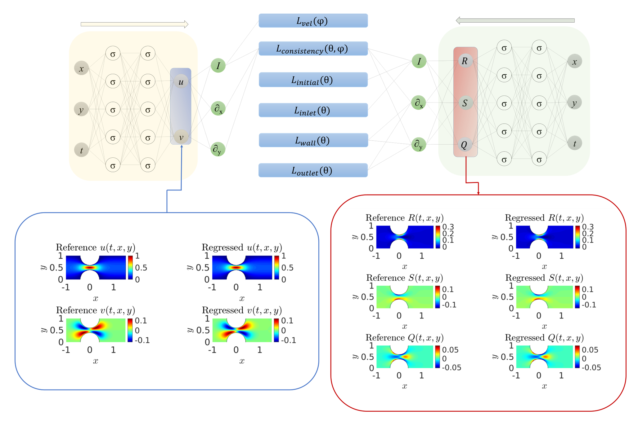
Figure 1: viscoelasticNet: To solve for the stress and learn the parameters of the general constitutive equation, we employ two fully connected neural networks with eight hidden layers and 128 neurons per hidden layer. The first network takes $x,y,t$ as inputs and outputs the $x$ and $y$ components of velocity ($u,v$). The second network takes $x,y,t$ as inputs and outputs the components of stress $R,S,Q$. The arrows at the top of the neural networks represent the direction of flow of information. We employ automatic differentiation to compute the losses described in section 2. Here $I$ denotes the identity operator, and we compute the differential operators $\partial t,\partial x,\partial y$ using automatic differentiation.

Figure 2: viscoelasticNet: To solve for the pressure, we employ a fully connected neural network with eight hidden layers and 64 neurons per hidden layer. The first network takes $x,y,z$ as inputs and outputs the pressure $p$. The arrows at the bottom of the neural networks represent the direction of flow of information. The velocity and stress components networks are the same as described in fig. 2. The parameters for the neural network for the stress are frozen when we solve for the pressure. We employ automatic differentiation to compute the losses described in section 2. Here, $I$ denotes the identity operator, and we compute the differential operators $\partial t,\partial x,\partial y$ using automatic differentiation.

2 Problem setup and methodology

2.1 Fluid motion equations

Consider an incompressible fluid under isothermal, single-phase, transient conditions. The following equations give the mass conservation and momentum balance in the absence of any body force

$$\nabla\cdot\boldsymbol{u}=0,$$ (1)

$$\rho\left(\frac{\partial\boldsymbol{u}}{\partial t}+\boldsymbol{u}\cdot\nabla\boldsymbol{u}\right)=-\nabla p+\nabla\cdot\boldsymbol{T^{\prime}},$$ (2)

where $\rho$ is the density of the fluid $\boldsymbol{u}$ is the velocity vector, $t$ is the time, $p$ is the pressure, and $\boldsymbol{T^{\prime}}$ is the stress tensor. In this work, we will represent scalars by non-bold characters, vectors by bold lowercase characters, and matrices by bold uppercase characters.

2.2 Rheological constitutive model

While solving for viscoelastic flows, the stress tensor $\boldsymbol{T}^{\prime}$ in equation (2) is often split into solvent and polymeric parts,

$$\boldsymbol{T^{\prime}}=\boldsymbol{T}^{s}+\boldsymbol{T}.$$ (3)

We need a constitutive relation for both the solvent and polymeric stress to have a well-posed problem. For a significant number of models, we can write the constitutive equations in the following form

$$\boldsymbol{T}^{s}=\nu(\nabla\boldsymbol{u}+\nabla\boldsymbol{u}^{T}),$$ (4)

$$f(\boldsymbol{T})\boldsymbol{T}+\lambda\overset{\nabla}{\boldsymbol{T}}+\boldsymbol{h}(\boldsymbol{T})=\eta(\nabla\boldsymbol{u}+\nabla\boldsymbol{u}^{T}),$$ (5)

where we denote the solvent viscosity by $\nu$ and the polymeric viscosity by $\eta$. the relaxation time by $\lambda$, the shear rate by $\dot{\gamma}$, $f(\boldsymbol{T})$ is a scalar-valued function, $\boldsymbol{h}(\boldsymbol{T})$ is a tensor-valued function and $\overset{\nabla}{\boldsymbol{T}}$ is the upper convected time derivative which is defined as

$$\overset{\nabla}{\boldsymbol{T}}=\frac{D\boldsymbol{T}}{Dt}-(\nabla\boldsymbol{u})^{T}\cdot\boldsymbol{T}-\boldsymbol{T}\cdot(\nabla\boldsymbol{u}),$$ (6)

where

$$\frac{D\boldsymbol{T}}{Dt}=\frac{\partial\boldsymbol{T}}{\partial t}+\boldsymbol{u}\cdot\nabla\boldsymbol{T}$$ (7)

is the material derivative. The principle of conservation of angular momentum implies that the polymetric stress tensor $\boldsymbol{T}$ is symmetric. Hence, we define the stress tensor $\boldsymbol{T}$ in two dimensions by three independent parameters

$$\boldsymbol{T}=\begin{bmatrix}R&S\\ S&Q\end{bmatrix},$$ (8)

where $R$ and $Q$ are the orthogonal normal stresses and $S$ is the orthogonal shear stress. This work considers the Oldroyd-B [37], Giesekus [38], and Linear PTT [39] models. The respective constitutive equations for the Oldroyd-B, Giesekus, and Linear PTT models are given by

$$\boldsymbol{T}+\lambda\overset{\nabla}{\boldsymbol{T}}=\eta(\nabla\boldsymbol{u}+\nabla\boldsymbol{u}^{T}),$$ (9)

$$\boldsymbol{T}+\lambda\overset{\nabla}{\boldsymbol{T}}+\alpha\frac{\lambda}{\eta}(\boldsymbol{T}\cdot\boldsymbol{T})=\eta(\nabla\boldsymbol{u}+\nabla\boldsymbol{u}^{T}),$$ (10)

and

$$\left(1+\frac{\epsilon\lambda}{\eta}tr(\boldsymbol{T})\right)\boldsymbol{T}+\lambda\overset{\nabla}{\boldsymbol{T}}=\eta(\nabla\boldsymbol{u}+\nabla\boldsymbol{u}^{T}),$$ (11)

where $tr(\boldsymbol{\tau})$ denotes the trace of the stress tensor and $\alpha$ is the mobility parameter. We can combine the three equations by writing a general form as

$$\left(1+\frac{\epsilon\lambda}{\eta}tr(\boldsymbol{T})\right)\boldsymbol{T}+\lambda\overset{\nabla}{\boldsymbol{T}}+\alpha\frac{\lambda}{\eta}(\boldsymbol{T}\cdot\boldsymbol{T})=\eta(\nabla\boldsymbol{u}+\nabla\boldsymbol{u}^{T}),$$ (12)

which we use to represent the Oldroyd-B, Giesekus, and Linear PTT models as shown in table 1. Equations 9, 10, 11, and 12 are special cases of Eq. 5.

Table 1: The list of parameters

in equation (12) to represent the Oldroyd-B, Giesekus, and Linear PTT models.

Model	$\epsilon$	$\alpha$
Oldroyd	$0$	$0$
Gieseukus	$0$	$\neq 0$
Linear PTT	$\neq 0$	$0$

2.3 Physics informed neural networks

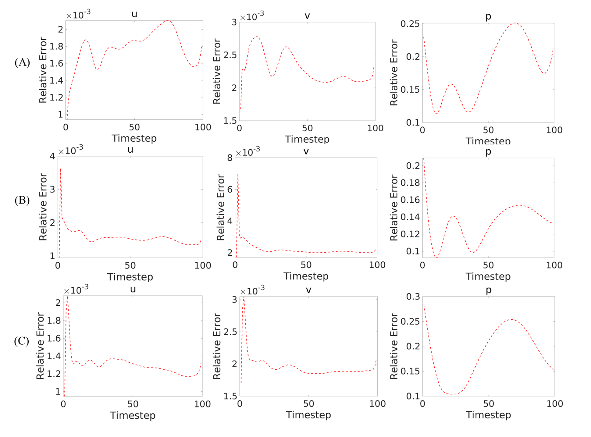
Figure 3: Relative errors between the predictions of the model and the corresponding reference velocity and pressure fields across the timesteps for (A) Oldroyd (B) Linear PTT (C) Giesekus constitutive model.

We develop a physics-informed neural network based framework called viscoelasticNet, which combines the information available in the velocity field, the Navier-Stokes equation, and the general form of the constitutive equation (12). The objective is to learn the parameters of the constitutive equation while simultaneously solving the forward problem of obtaining the stress field. We consider the velocity field $\textbf{u}(t,x,y)=[u(t,x,y),v(t,x,y)$] of an incompressible isothermal flow of a viscoelastic fluid. We observe N data points of time-space coordinates ($t_{n},x_{n},y_{n}$) and the velocity of the fluid corresponding to these points ($u_{n},v_{n}$) where $n=1,\ldots,N$. Given such scattered spatio-temporal data, we are interested in the discovery of the components of the stress tensor $R(t,x,y)$, $S(t,x,y)$ and $Q(t,x,y)$ as well as their governing equation by determining the parameters $\epsilon,\lambda,\alpha,\eta$ and $\nu$ in Eq. (12). Our setup has absolutely no input data on the pressure field and the stress tensor, except for the initial and boundary conditions.

In our setup, we treat the $x$ and $y$ components of the velocity, the value of the stress field at the first time step (initial value), the stress field at the inlet, and the value of the pressure field as the observables. We approximate the functions $(t,x,y)\longmapsto(R,S,Q)$, $(t,x,y)\longmapsto\psi$ and $(t,x,y)\longmapsto p$ using three deep neural networks with parameters $\theta$, $\phi$ and $\kappa$, respectively. For the $x$-component of velocity $u(t,x,y)$ and $y$-component $v(t,x,y)$, we make the assumption that

$$u=\psi_{y},v=-\psi_{x},$$ (13)

for some latent function $\psi(t,x,y)$. This approach can be extended to three dimensions as well. The velocity field then automatically satisfies the continuity equation (1). We decouple the momentum equations of the Navier-Stokes from the constitutive equations for the polymeric stress and solve them in a sequential manner. We chose a separate network for pressure as, in our experience, this setup worked better with our decoupled sequential approach. We define the mean squared error loss for regression over the velocity field as

$$L_{vel}(\phi)=\mathbb{E}_{(t,x,y,u,v)}[\frac{|{u}(t,x,y;\phi)-{u}|^{2}}{{\sigma_{u}}^{2}}]+\mathbb{E}_{(t,x,y,u,v)}[\frac{|{v}(t,x,y;\phi)-{v}|^{2}}{{\sigma_{v}}^{2}}],$$ (14)

where ${\sigma_{u}}$ and ${\sigma_{v}}$ are the standard deviation of the $x$ and $y$ components of the reference velocity field, and $\mathbb{E}$ denotes the expectation approximated by the population mean (i.e., mean of the observations $t_{n},x_{n},y_{n},u_{n},v_{n}$).

Since we are also solving the forward problem of learning the stress field, initial and boundary conditions on the stress field are required. We then solve the governing equation with the Dirichlet boundary condition at the inlet and Neumann boundary condition at the walls and the outlet. We enforce the initial condition using the loss function

$$\begin{split}L_{init}(\theta)=&\mathbb{E}_{(t^{init},x^{init},y^{init},{R}^{init})}[\frac{|{R}(t^{init},x^{init},y^{init};\theta)-{R}^{init}|^{2}}{{\sigma_{R}}^{2}}]+\\ &\mathbb{E}_{(t^{init},x^{init},y^{init},{S}^{init})}[\frac{|{S}(t^{init},x^{init},y^{init};\theta)-{S}^{init}|^{2}}{{\sigma_{S}}^{2}}]+\\ &\mathbb{E}_{(t^{init},x^{init},y^{init},{Q}^{init})}[\frac{|{Q}(t^{init},x^{init},y^{init};\theta)-{Q}^{init}|^{2}}{{\sigma_{Q}}^{2}}],\end{split}$$ (15)

where $t^{init},x^{init},y^{init}$ is the spatio-temporal point cloud at the initial timestep, $R^{init}$, $S^{init}$ and $Q^{init}$ are the components of the stress field at the first time step $t^{init}$ and ${\sigma_{R}}$, ${\sigma_{S}}$ and ${\sigma_{Q}}$ are the respective standard deviations of $R^{init}$, $S^{init}$ and $Q^{init}$. To enforce the Neumann boundary conditions, we use the normal vectors for the wall ($\boldsymbol{n^{w}}=(l^{w},m^{w})$) and the outlet ($\boldsymbol{n^{o}}=(l^{o},m^{o})$). We enforce the boundary conditions at the wall using

$$\begin{split}L_{wall}(\theta)=&\mathbb{E}_{(t^{w},x^{w},y^{w},l^{w},m^{w})}[|R_{x}(t^{w},x^{w},y^{w};\theta){l}^{w}+R_{y}(t^{w},x^{w},y^{w};\theta){m}^{w}|^{2}]+\\ &\mathbb{E}_{(t^{w},x^{w},y^{w},l^{w},m^{w})}[|S_{x}(t^{w},x^{w},y^{w};\theta){l}^{w}+S_{y}(t^{w},x^{w},y^{w};\theta){m}^{w}|^{2}]+\\ &\mathbb{E}_{(t^{w},x^{w},y^{w},l^{w},m^{w})}[|Q_{x}(t^{w},x^{w},y^{w};\theta){l}^{w}+Q_{y}(t^{w},x^{w},y^{w};\theta){m}^{w}|^{2}],\end{split}$$ (16)

where $t^{w},x^{w},y^{w}$ is the spatio-temporal point cloud on the walls of the domain, and $l^{w}$ and $m^{w}$ are the $x$ and $y$ components of the corresponding normal vector. We enforce the boundary condition at the outlet using

$$\begin{split}L_{outlet}(\theta)=&\mathbb{E}_{(t^{o},x^{o},y^{o},l^{o},m^{o})}[|R_{x}(t^{o},x^{o},y^{o};\theta){l}^{o}+R_{y}(t^{o},x^{o},y^{o};\theta){m}^{o}|^{2}]+\\ &\mathbb{E}_{(t^{o},x^{o},y^{o},l^{o},m^{o})}[|S_{x}(t^{o},x^{o},y^{o};\theta){l}^{o}+S_{y}(t^{o},x^{o},y^{o};\theta){m}^{o}|^{2}]+\\ &\mathbb{E}_{(t^{o},x^{o},y^{o},l^{o},m^{o})}[|Q_{x}(t^{o},x^{o},y^{o};\theta){l}^{o}+Q_{y}(t^{o},x^{o},y^{o};\theta){m}^{o}|^{2}],\end{split}$$ (17)

where $t^{o},x^{o},y^{o}$ is the spatio-temporal point cloud on the outlet of the domain, and $l^{o}$ and $m^{o}$ are the $x$ and $y$ components of the corresponding normal vector. For the Dirichlet boundary condition at the inlet, we have

$$\begin{split}L_{inlet}(\theta)=&\mathbb{E}_{(t^{i},x^{i},y^{i},{R}^{i})}[\frac{|{R}(t^{i},x^{i},y^{i};\theta)-{R}^{i}|^{2}}{{\sigma_{R}}^{2}}]+\\ &\mathbb{E}_{(t^{i},x^{i},y^{i},{S}^{i})}[\frac{|{S}(t^{i},x^{i},y^{i};\theta)-{S}^{i}|^{2}}{{\sigma_{S}}^{2}}]+\\ &\mathbb{E}_{(t^{i},x^{i},y^{i},{Q}^{i})}[\frac{|{Q}(t^{i},x^{i},y^{i};\theta)-{Q}^{i}|^{2}}{{\sigma_{Q}}^{2}}],\end{split}$$ (18)

where $t^{i},x^{i},y^{i}$ is the spatio-temporal point cloud at the inlet of the domain, $R^{i}$, $S^{i}$ and $Q^{i}$ are the components of the stress field at the inlet. Now, let

$$\begin{split}f^{R}(t,x,y,;\theta,\phi)=&uR_{x}+vR_{y}-2(Ru_{x}+Su_{y})+\frac{\alpha}{\eta}(R^{2}+S^{2})\\ &+\left(\frac{1}{\lambda}+\frac{\epsilon}{\eta}(R+Q)\right)R-\frac{2\eta}{\lambda}u_{x},\end{split}$$ (19)

$$\begin{split}f^{S}(t,x,y,;\theta,\phi)=&uS_{x}+vS_{y}-(Rv_{x}+Su_{y})+\frac{\alpha}{\eta}(S(R+Q))\\ &+\left(\frac{1}{\lambda}+\frac{\epsilon}{\eta}(R+Q)\right)S-\frac{\eta}{\lambda}(u_{y}+v_{x}),\end{split}$$ (20)

$$\begin{split}f^{Q}(t,x,y,;\theta,\phi)=&uQ_{x}+vQ_{y}-2(Sv_{x}+Qv_{y})+\frac{\alpha}{\eta}(S^{2}+Q^{2})\\ &+\left(\frac{1}{\lambda}+\frac{\epsilon}{\eta}(R+Q)\right)Q-\frac{2\eta}{\lambda}v_{y}.\end{split}$$ (21)

We then create a physics-informed neural network using the backward Euler discretization

$$\begin{split}R^{pi}(t,x,y;\Delta t,\theta)=R^{pu}(t+\Delta t,x,y;\theta)-\Delta tf^{R}(&R^{pu}(t+\Delta t,x,y;\theta),\\ &S^{pu}(t+\Delta t,x,y;\theta),\\ &Q^{pu}(t+\Delta t,x,y;\theta);\\ &u,v,\lambda,\epsilon,\eta),\end{split}$$ (22)

$$\begin{split}S^{pi}(t,x,y;\Delta t,\theta)=S^{pu}(t+\Delta t,x,y;\theta)-\Delta tf^{S}(&R^{pu}(t+\Delta t,x,y;\theta),\\ &S^{pu}(t+\Delta t,x,y;\theta),\\ &Q^{pu}(t+\Delta t,x,y;\theta);\\ &u,v,\lambda,\epsilon,\eta),\end{split}$$ (23)

$$\begin{split}Q^{pi}(t,x,y;\Delta t,\theta)=Q^{pu}(t+\Delta t,x,y;\theta)-\Delta tf^{Q}(&R^{pu}(t+\Delta t,x,y;\theta),\\ &S^{pu}(t+\Delta t,x,y;\theta),\\ &Q^{pu}(t+\Delta t,x,y;\theta);\\ &u,v,\lambda,\epsilon,\eta).\end{split}$$ (24)

Since the physics-informed and uninformed networks evaluate the stress at the same point ${t,x,y}$, they need to be consistent. We enforce this using a consistency loss

$$\begin{split}L_{consistency}(\theta;\Delta t)=&\mathbb{E}_{(t,x,y)}[\frac{|{R}^{pi}(t,x,y;\Delta t,\theta)-{R}^{pu}(t,x,y;\theta)|^{2}}{{\sigma_{R}}^{2}}]+\\ &\mathbb{E}_{(t,x,y)}[\frac{|{S}^{pi}(t,x,y;\Delta t,\theta)-{S}^{pu}(t,x,y;\theta)|^{2}}{{\sigma_{S}}^{2}}]+\\ &\mathbb{E}_{(t,x,y)}[\frac{|{Q}^{pi}(t,x,y;\Delta t,\theta)-{Q}^{pu}(t,x,y;\theta)|^{2}}{{\sigma_{Q}}^{2}}],\end{split}$$ (25)

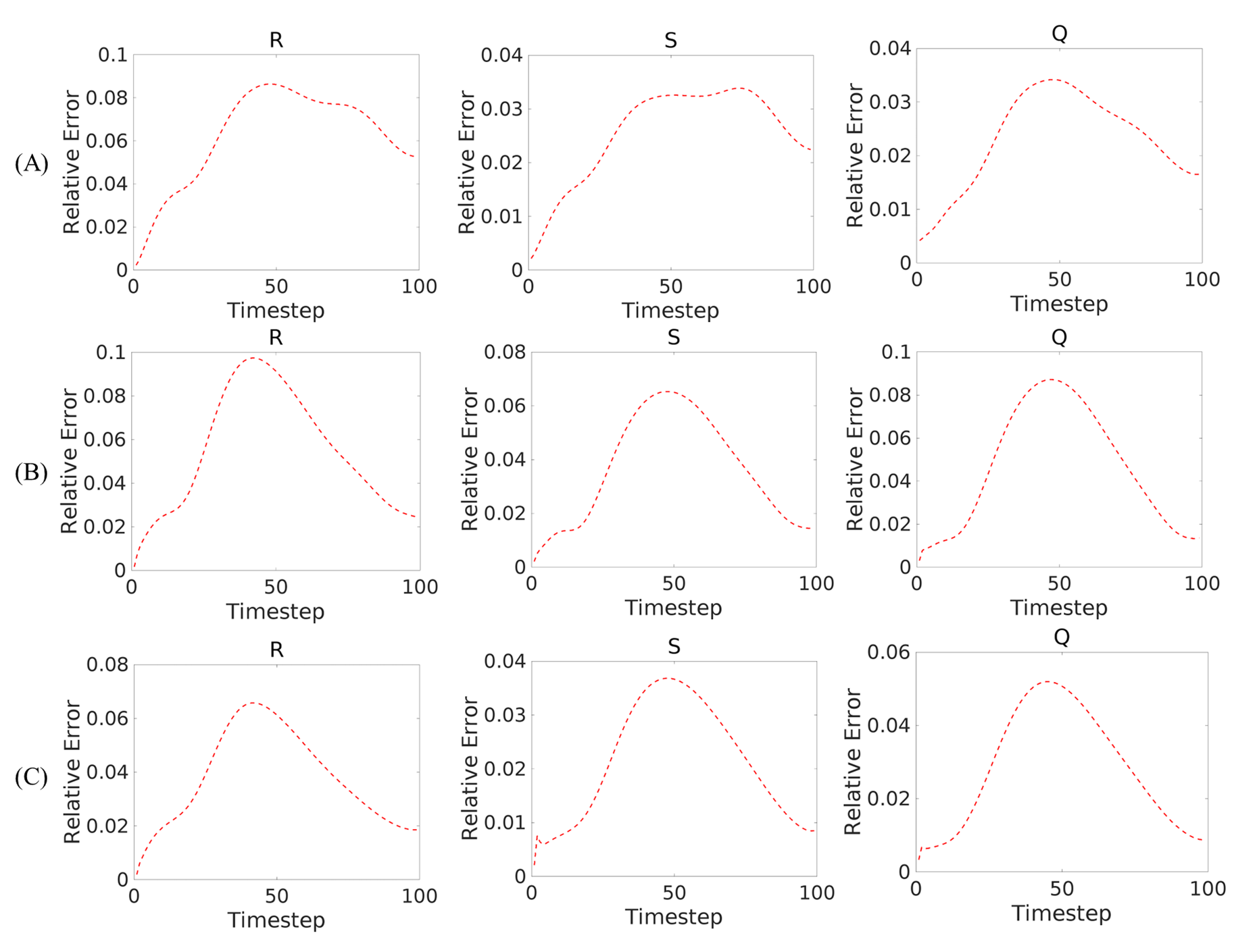
Figure 4: Relative errors between the predictions of the model and the corresponding reference components of the stress field across timesteps for (A) Oldroyd (B) Linear PTT (C) Giesekus constitutive models.

The parameters $\theta$ and $\phi$ are then optimized to minimize the following combined loss

$$\begin{split}L_{stress}(\theta,\phi)=&L_{vel}(\phi)+L_{initial}(\theta)+L_{wall}(\theta)+\\ &L_{outlet}(\theta)+L_{inlet}(\theta)+L_{consistency}(\theta,\phi).\end{split}$$ (26)

We show the setup scheme in figure 2. Regularization is a practice used to avoid overfitting in machine learning. We use our prior knowledge of the governing equations to regularize the optimization process of the neural network parameters. Since we are sequentially solving the problem, we freeze the optimized parameters $\theta^{\prime}$ while solving for pressure. We split the momentum equation (2) into two parts, one which can be directly computed from the observables and the second which has unknown components. The first part is given by

$$\begin{split}g^{L}(u,v)=u_{t}+uu_{x}+vu_{y},\\ h^{L}(u,v)=v_{t}+uv_{x}+vv_{y},\end{split}$$ (27)

and

$$\begin{split}g^{R}(p;u,v,R,S,\nu)=-p_{x}+\nu(u_{xx}+u_{yy})+(R_{x}+S_{y}),\\ h^{R}(p;u,v,S,Q,\nu)=-p_{y}+\nu(v_{xx}+v_{yy})+(S_{x}+Q_{y}).\end{split}$$ (28)

We calculate the standard deviation of ${g}^{L}$ and ${h}^{L}$ as ${\sigma_{g}}$ and ${\sigma_{h}}$, respectively. We then enforce the momentum equations (Eq. (2)) using

$$\begin{split}K_{m}(\phi,\kappa)&=\mathbb{E}_{(t,x,y)}\left[\dfrac{\left|\displaystyle\begin{multlined}g^{L}(u(t,x,y;\phi))-g^{R}(p(t,x,y;\kappa);u(t,x,y;\phi),\\ v(t,x,y;\phi),R(t,x,y;\theta^{\prime}),S(t,x,y;\theta^{\prime}),\nu)\end{multlined}g^{L}(u(t,x,y;\phi))-g^{R}(p(t,x,y;\kappa);u(t,x,y;\phi),\\ v(t,x,y;\phi),R(t,x,y;\theta^{\prime}),S(t,x,y;\theta^{\prime}),\nu)\right|^{2}}{\sigma_{g}^{2}}\right]\\ &+\mathbb{E}_{(t,x,y)}\left[\dfrac{\left|\displaystyle\begin{multlined}h^{L}(u(t,x,y;\phi))-h^{R}(p(t,x,y;\kappa);u(t,x,y;\phi),\\ v(t,x,y;\phi),S(t,x,y;\theta^{\prime}),Q(t,x,y;\theta^{\prime}),\nu)\end{multlined}h^{L}(u(t,x,y;\phi))-h^{R}(p(t,x,y;\kappa);u(t,x,y;\phi),\\ v(t,x,y;\phi),S(t,x,y;\theta^{\prime}),Q(t,x,y;\theta^{\prime}),\nu)\right|^{2}}{\sigma_{h}^{2}}\right].\end{split}$$ (29)

We enforce the Neumann boundary conditions on the wall for the pressure as

$$K_{wall}(\kappa)=\mathbb{E}_{(t^{w},x^{w},y^{w},{l}^{w},{m}^{w})}[|p_{x}(t^{w},x^{w},y^{w};\kappa){l}^{w}+p_{y}(t^{w},x^{w},y^{w};\kappa){m}^{w}|^{2}],$$ (30)

where $t^{w},x^{w},y^{w}$ is the spatio-temporal point cloud on the walls of the domain, and $l^{w}$ and $m^{w}$ are the $x$ and $y$ components of the corresponding normal vector. To enforce the Neumann boundary conditions, we use the normal vectors for the inlet ($\boldsymbol{n^{i}}=(l^{i},m^{i})$). For the inlet, we enforce

$$K_{inlet}(\kappa)=\mathbb{E}_{(t^{i},x^{i},y^{i},l^{i},m^{i})}[|p_{x}(t^{i},x^{i},y^{i};\kappa){l}^{i}+p_{y}(t^{i},x^{i},y^{i};\kappa){m}^{i}|^{2}],$$ (31)

where $t^{i},x^{i},y^{i}$ is the spatio-temporal point cloud on the inlet of the domain, and $l^{i}$ and $m^{i}$ are the $x$ and $y$ components of the corresponding normal vector. For the Dirichlet boundary condition at the outlet for the pressure, we have

$$K_{outlet}(\kappa)=\mathbb{E}_{(t^{o},x^{o},y^{o},p^{o})}[|{p(t^{o},x^{o},y^{o};\kappa)-p^{o}}|^{2}],$$ (32)

where {$t^{o},x^{o},y^{o}$} are spatio-temporal points at the outlet and ${p}^{o}$ is the pressure field at the outlet. We do not divide by the standard deviation of the pressure as the pressure is zero at the outlet in our case. We optimize the parameters $\phi$ and $\kappa$ using the following combined loss

$$K_{pressure}(\phi,\kappa)=L_{vel}(\phi)+K_{mom}(\phi,\kappa)+K_{wall}(\kappa)+K_{inlet}(\kappa)+K_{outlet}(\kappa).$$ (33)

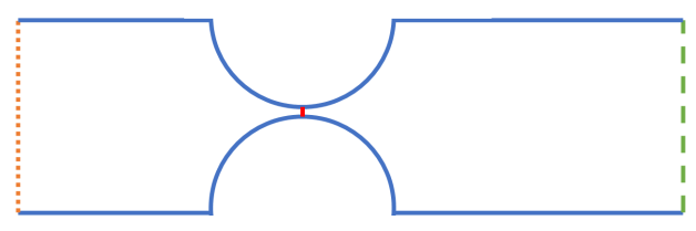
Figure 5: A two-dimensional stenosis. We show the domain walls using solid blue curves, the inlet with a dotted orange line, and the outlet with a dashed green line. The narrowest part of the throat of the stenosis is highlighted with a red line. We plot the stress in this region in Fig. 6.

3 Results

We consider a two-dimensional simplified geometry of stenosis, as shown in Fig. 5. We used RheoTool [40], an OpenFOAM [41] based open source software developed on the work by Favero et al. [42] to generate the training and reference data sets. RheoTool uses the finite volume method to discretize the equations. It uses the both-side-diffusion technique to increase the ellipticity which stabilizes the momentum equation. We use the log-confirmation tensor approach to tackle the numerical instabilities in the polymeric stress. More details on the solver and the validation for the code can be found here [40, 42]. The input to the algorithm essentially is the velocity field and the boundary conditions on stress and pressure. For all the results discussed in this section, we represent the components of velocity ($u,v$) using an eight-layer deep, fully connected neural network with 128 neurons per hidden layer. We represent the stress components ($R,S,Q$) with another eight layers deep, fully connected neural network with 128 neurons per hidden layer. We use a third neural network to represent the pressure ($p$) with an eight-layer deep, fully connected neural network with 64 neurons per hidden layer. We use the swish function as the activation function for all the networks. There might be other architectures that can improve the results presented in this section.

Table 2: Relative error for flow variables at different noise levels for the Oldroyd-B model

	$u$	$v$	$p$
0% Noise	$1.6\times 10^{-3}$	$2.2\times 10^{-3}$	$1.94\times 10^{-1}$
1% Noise	$1.7\times 10^{-3}$	$2.3\times 10^{-3}$	$2.02\times 10^{-1}$
5% Noise	$1.7\times 10^{-3}$	$2.4\times 10^{-3}$	$1.87\times 10^{-1}$
10% Noise	$1.8\times 10^{-3}$	$2.6\times 10^{-3}$	$1.69\times 10^{-1}$

Table 3: Relative error for the stress components at different noise levels for the Oldroyd-B model

	$R$	$S$	$Q$
0% Noise	$5.99\times 10^{-2}$	$2.45\times 10^{-2}$	$2.28\times 10^{-2}$
1% Noise	$5.93\times 10^{-2}$	$2.48\times 10^{-2}$	$2.31\times 10^{-2}$
5% Noise	$5.94\times 10^{-2}$	$2.47\times 10^{-2}$	$2.10\times 10^{-2}$
10% Noise	$6.02\times 10^{-2}$	$2.55\times 10^{-2}$	$2.36\times 10^{-2}$

Table 4: Sensitivity to noise level in the velocity data for the Oldroyd model

	$\alpha$	$\epsilon$	$\lambda$	$\eta$	$\nu$
Reference value	$0.00$	$0.0$	$0.05$	$0.008$	$0.01$
0% noise	$0.00$	$0.0$	$0.0517$	$0.0081$	$0.0098$
1% noise	$0.00$	$0.0$	$0.0517$	$0.0081$	$0.0115$
5% noise	$0.00$	$0.0$	$0.0517$	$0.0081$	$0.0115$
10% noise	$0.00$	$0.0$	$0.0517$	$0.0081$	$0.0112$

Table 5: Relative error for flow variables at different noise levels for the linear PTT model

	$u$	$v$	$p$
0% Noise	$1.6\times 10^{-3}$	$2.2\times 10^{-3}$	$1.33\times 10^{-1}$
1% Noise	$1.8\times 10^{-3}$	$2.4\times 10^{-3}$	$1.69\times 10^{-1}$
5% Noise	$1.9\times 10^{-3}$	$2.6\times 10^{-3}$	$1.77\times 10^{-1}$
10% Noise	$2.2\times 10^{-3}$	$3\times 10^{-3}$	$1.85\times 10^{-1}$

Table 6: Relative error for the stress components at different noise levels for the linear PTT model

	$R$	$S$	$Q$
0% Noise	$5.45\times 10^{-2}$	$3.64\times 10^{-2}$	$4.62\times 10^{-2}$
1% Noise	$5.65\times 10^{-2}$	$3.77\times 10^{-2}$	$4.7\times 10^{-2}$
5% Noise	$5.66\times 10^{-2}$	$3.82\times 10^{-2}$	$4.75\times 10^{-2}$
10% Noise	$5.91\times 10^{-2}$	$3.97\times 10^{-2}$	$4.78\times 10^{-2}$

Table 7: Sensitivity to the noise level in the velocity data for the linear PTT model

Model parameters	$\alpha$	$\epsilon$	$\lambda$	$\eta$	$\nu$
True value	$0.00$	$0.1$	$0.15$	$0.015$	$0.01$
0% noise	$0.00$	$0.106$	$0.161$	$0.0157$	$0.0097$
1% noise	$0.00$	$0.108$	$0.162$	$0.0157$	$0.0123$
5% noise	$0.00$	$0.108$	$0.162$	$0.0157$	$0.0123$
10% noise	$0.00$	$0.108$	$0.161$	$0.0157$	$0.0127$

Table 8: Relative error for flow variables at different noise levels for the Giesekus model

	$u$	$v$	$p$
0% Noise	$1.3\times 10^{-3}$	$2.0\times 10^{-3}$	$1.95\times 10^{-1}$
1% Noise	$1.4\times 10^{-3}$	$2.1\times 10^{-3}$	$1.82\times 10^{-1}$
5% Noise	$1.4\times 10^{-3}$	$2.2\times 10^{-3}$	$1.83\times 10^{-1}$
10% Noise	$1.7\times 10^{-3}$	$2.5\times 10^{-3}$	$1.77\times 10^{-1}$

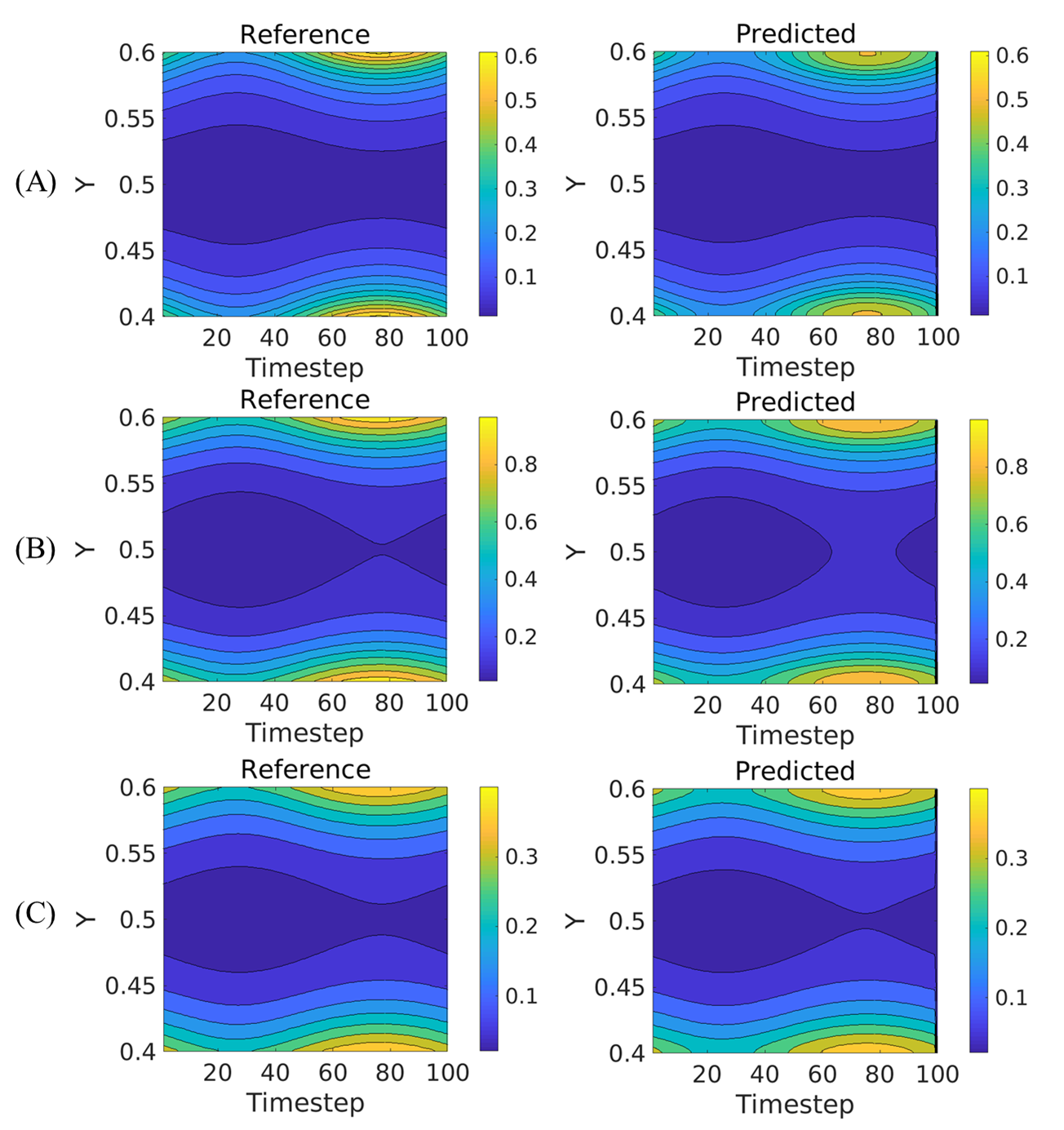
Figure 6: Comparison of the reference and predicted magnitude of the stress in the throat of the stenosis across all the timesteps for (A) Oldroyd (B) Linear PTT (C) Giesekus constitutive models. The first column shows the reference values, and the second column shows the model’s predictions.

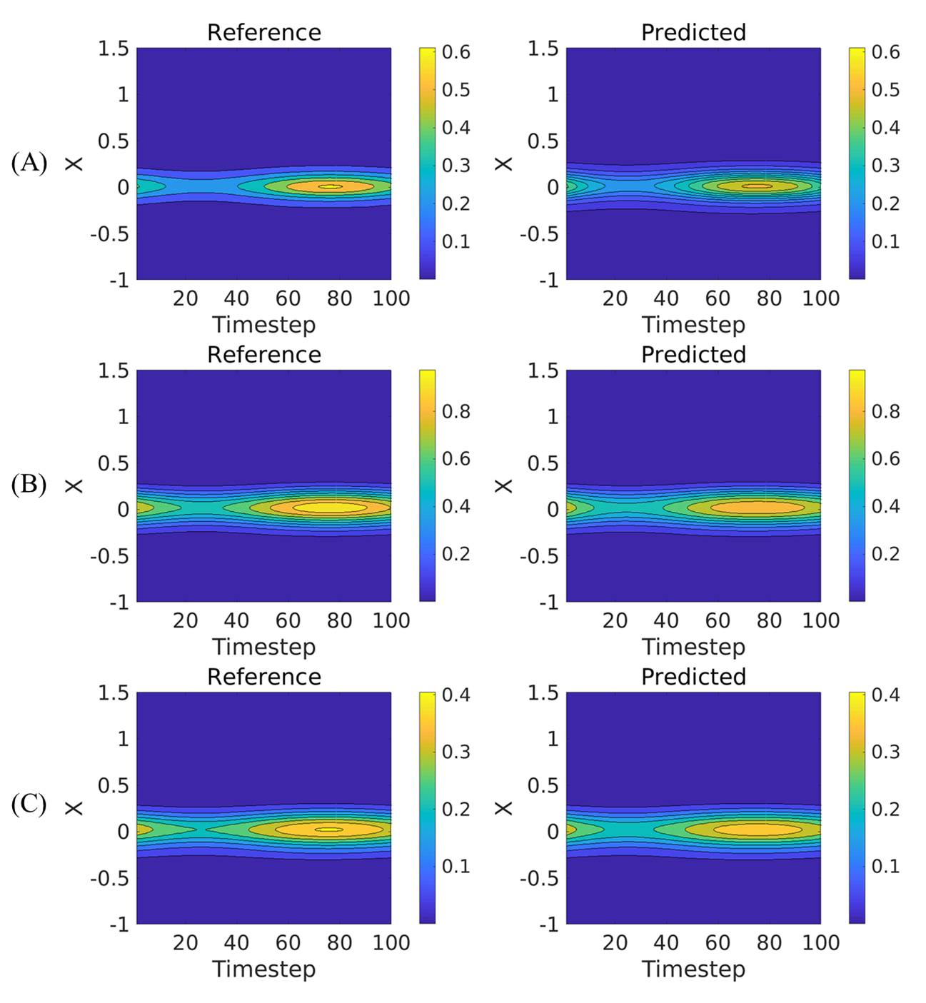
Figure 7: Comparison of the reference and predicted magnitude of the stress on the lower wall across all the timesteps for (A) Oldroyd (B) Linear PTT (C) Giesekus constitutive models. The first column shows the reference values, and the second column shows the model’s predictions.

The learning rate schedule is an important hyperparameter that determines how well the network parameters are optimized. For all the results reported in this work, we use a cosine annealing learning rate schedule [43]. We used a value of $2.5E-03$ for $\zeta_{max}$ and $2.5E-06$ for $\zeta_{min}$ to get the learning rate $\zeta$ as defined in the following equation

$$\zeta=\zeta_{min}+0.5(\zeta_{max}-\zeta_{min})\left(1+cos\left(\frac{T_{cur}}{T_{max}}\pi\right)\right),$$ (34)

where $T_{cur}$ is the current time step and $T_{max}$ is the total timestep. For learning the parameters in the general equation (12) and the stress field, two million iterations of the Adam optimizer [44] were used. We chose the mini-batch size to be 256 for the spatio-temporal point cloud inside the domain and 64 for all the points on the boundary. Every ten iterations of the Adam optimizer took around 0.45 seconds. As we solve for the pressure sequentially, we first optimize the parameters of the neural network for the stress ($\theta$) by minimizing the loss function defined in Eq. (26) and freezing them. We then optimize the parameters for the neural network for velocity ($\phi$) and pressure ($\kappa$) by minimizing the loss specified in equation (33). For this optimization process, we ran 800,000 iterations of the Adam optimizer with the same learning rate schedule defined above.

We consider the geometry of a 2D stenosis as shown in figure 5 for all the results discussed in this section. While generating the reference data-set, we applied a sinusoidal boundary condition for the velocity on the inlet. The simulation ran for a hundred time steps, or half a sine wave ( 0 to $\pi$). As discussed in section 2, we choose a sequential approach to solve for the stress and the pressure. Given the initial and boundary conditions on the stress, we are simultaneously solving the inverse problem of learning the parameters of the general equation (12) and the forward problem of discovering the stress field in the spatio-temporal domain. To compare the results predicted by the neural networks to the reference value and simulation results, we defined the relative error to be

$$\mathcal{L}(a_{reference},a_{prediction})=\sqrt{\frac{\overline{(a_{reference}-a_{prediction})^{2}}}{\overline{(a_{reference}-\bar{a}_{reference})^{2}}}},$$ (35)

where the bar denotes the mean value. We use this definition for error so that the multiplication or addition of a constant does not change it. We show the relative error between the regressed and reference values for the velocity, pressure, and stress fields in Fig. 3 and Fig. 4. As expected, the lowest errors are for the velocity fields as there is data on those fields. The lowest error in the stress fields is on the first step, as the initial condition is regressed.

In Fig. 6, we plot the reference and predicted values of the magnitude of the stress in the throat of the stenosis across all the time steps. Although there is an excellent qualitative and quantitative agreement between the predicted and reference values, the model seems to be under-predicting the magnitude of the stress on the walls. To focus on the walls, in Fig. 7, we plot the reference and predicted value of the magnitude of stress on the lower wall across all the time steps for the Oldroyd, Linear PTT, and Giesekus models. The stress magnitude on the lower and upper walls are symmetric; We, therefore, show the results of only the lower wall. The predictions for the Giesekus model seem to be performing best. There is an excellent qualitative and quantitative agreement between the reference and predicted values. However, the model seems to be under-predicting the peak value in all the cases. Furthermore, our framework appears to perform best for the Giesekus model among the three models.

To check the robustness of our framework, we add Gaussian noise to the velocity observations. The effect of noise on the parameters for the Oldroyd-B, linear PTT and Giesekus models are reported in the tables 4,7 and 10, respectively. We notice that adding a Gaussian noise does not significantly affect the parameters learned for Eq. (12). However, there is an increase in the error for the learned viscosity $\nu$. Interestingly, the error does not increase as we increase the amount of Gaussian noise. The error for the learnt velocity, pressure and stress components for the Oldroyd-B, linear PTT and Giesekus models are reported in tables 2, 3, 5, 6, 8 and 9. The general trend is that the error for each variable increases slightly as the noise level increases, but the increase in error is not significant.

We believe that this low sensitivity to the Gaussian noise occurs because there are too many data points for the model. The models were trained on 5.78 million spatio temporal data points of velocity till now. We tried training our model on fewer data points to test this hypothesis. Specifically, we consider the Giesekus model with 5.78 million, 578 thousand, 57.8 thousand, and 5.78 thousand data points with 5% Gaussian noise in the velocity data. The results for the parameters are summarized in Table 11. The results start to deteriorate at about 57.8 thousand points, with the value for viscosity ($\nu$) being off by about 50%. The model fails to learn the viscosity ($\nu$) with 5.78 thousand spatio-temporal points but still learns the parameters of the general equation (Eq. 12) reasonably well. Given these results, we can conclude that the model is fairly robust and works well with noisy and sparse data sets.

Table 9: Relative error for the stress components at different noise levels for the Giesekus model

	$R$	$S$	$Q$
0% Noise	$3.88\times 10^{-2}$	$2.16\times 10^{-2}$	$2.88\times 10^{-2}$
1% Noise	$3.75\times 10^{-2}$	$2.12\times 10^{-2}$	$2.83\times 10^{-2}$
5% Noise	$3.83\times 10^{-2}$	$2.17\times 10^{-2}$	$2.89\times 10^{-2}$
10% Noise	$3.85\times 10^{-2}$	$2.19\times 10^{-2}$	$2.89\times 10^{-2}$

Table 10: Sensitivity to the noise level in the velocity data for the Gieseukus model

	$\alpha$	$\epsilon$	$\lambda$	$\eta$	$\nu$
Reference value	$0.2$	$0.0$	$0.1$	$0.01$	$0.01$
0% noise	$0.205$	$0.0$	$0.105$	$0.0094$	$0.0103$
1% noise	$0.205$	$0.0$	$0.105$	$0.0098$	$0.0103$
5% noise	$0.205$	$0.0$	$0.105$	$0.0097$	$0.0103$
10% noise	$0.205$	$0.0$	$0.105$	$0.0099$	$0.0103$

Table 11: Sensitivity to amount of spatio-temporal data

	$\alpha$	$\epsilon$	$\lambda$	$\eta$	$\nu$
Reference value	$0.2$	$0.0$	$0.1$	$0.01$	$0.01$
5.78 million	$0.205$	$0.0$	$0.105$	$0.0097$	$0.0103$
578 thousand	$0.205$	$0.0$	$0.105$	$0.0103$	$0.0093$
57.8 thousand	$0.206$	$0.0$	$0.106$	$0.0103$	$0.0155$
5.78 thousand	$0.217$	$0.0$	$0.111$	$0.0104$	$0.00045$

4 Conclusions and future scope of work

We introduce viscoelasticNet, a physics-informed neural networks (PINNs)-based framework that can select the viscoelastic constitutive model and learn the stress field from a velocity flow field. In this work, we work with three commonly used non-linear viscoelastic models: the Oldroyd-B, Giesekus, and Linear PTT, and build a generalized framework to model them. The velocity, pressure, and stress fields are represented using neural networks. The backward Euler method was used to construct PINNs for the viscoelastic constitutive model. We use a multistage approach to solve the problem by first solving for the stress and then using the stress field and the velocity field to solve for the pressure. To test our framework, we used noisy and sparse data sets in this work. We observed that the framework could learn the parameters of the viscoelastic constitutive model reasonably well in all the cases.

In this work, we worked with a stenosis geometry in two dimensions with the above-mentioned constitutive models. This framework can also be extended to include more sophisticated rheological constitutive models. More complex geometries and three-dimensional cases can be considered for future work. The framework presented here can be used to augment techniques like particle image velocimetry (PIV). While PIV can be used to acquire the velocity flow field, the pressure and stress fields can be acquired using our method. Moreover, once the constitutive equation is learned, the parameters can be used to model any future applications of the pertinent fluid.

5 Acknowledgements

A.M.A. acknowledges financial support from the National Science Foundation (NSF) through Grant No. CBET-2141404.

References

-
[1]
G. Li, E. Lauga, A. M. Ardekani,
Microswimming in
viscoelastic fluids, Journal of Non-Newtonian Fluid Mechanics 297 (April)
(2021) 104655.
doi:10.1016/j.jnnfm.2021.104655.
URL https://doi.org/10.1016/j.jnnfm.2021.104655 - [2] C. K. Tung, C. Lin, B. Harvey, A. G. Fiore, F. Ardon, M. Wu, S. S. Suarez, Fluid viscoelasticity promotes collective swimming of sperm, Scientific Reports 7 (1) (2017) 1–9. doi:10.1038/s41598-017-03341-4.
- [3] G. Li, A. M. Ardekani, Collective Motion of Microorganisms in a Viscoelastic Fluid, Physical Review Letters 117 (11) (2016) 1–5. doi:10.1103/PhysRevLett.117.118001.
- [4] G. J. Li, A. Karimi, A. M. Ardekani, Effect of solid boundaries on swimming dynamics of microorganisms in a viscoelastic fluid, Rheologica Acta 53 (12) (2014) 911–926. doi:10.1007/s00397-014-0796-9.
- [5] R. Hu, S. Tang, M. Mpelwa, Z. Jiang, S. Feng, Research progress of viscoelastic surfactants for enhanced oil recovery, Energy Exploration and Exploitation 39 (4) (2021) 1324–1348. doi:10.1177/0144598720980209.
- [6] B. Wei, L. Romero-Zerón, D. Rodrigue, Oil displacement mechanisms of viscoelastic polymers in enhanced oil recovery (EOR): a review, Journal of Petroleum Exploration and Production Technology 4 (2) (2014) 113–121. doi:10.1007/s13202-013-0087-5.
- [7] M. A. Alves, P. J. Oliveira, F. T. Pinho, Numerical Methods for Viscoelastic Fluid Flows, Annual Review of Fluid Mechanics 53 (2021) 509–541. doi:10.1146/annurev-fluid-010719-060107.
- [8] J. G. Beijer, J. L. Spoormaker, Solution strategies for FEM analysis with nonlinear viscoelastic polymers, Computers and Structures 80 (14-15) (2002) 1213–1229. doi:10.1016/S0045-7949(02)00089-5.
-
[9]
P. Areias, K. Matouš,
Finite element
formulation for modeling nonlinear viscoelastic elastomers, Computer
Methods in Applied Mechanics and Engineering 197 (51-52) (2008) 4702–4717.
doi:10.1016/j.cma.2008.06.015.
URL http://dx.doi.org/10.1016/j.cma.2008.06.015 - [10] S. Wang, Z. Su, L. Ying, X. Peng, S. Zhu, F. Liang, D. Feng, D. Liang, I. Technologies, ACCELERATING MAGNETIC RESONANCE IMAGING VIA DEEP LEARNING Paul C . Lauterbur Research Center for Biomedical Imaging , SIAT , CAS , Shenzhen , P . R . China Department of Biomedical Engineering and Department of Electrical Engineering , The State Universit, Isbi 2016 (2016) 514–517.
- [11] S. Min, B. Lee, S. Yoon, Deep learning in bioinformatics, Briefings in bioinformatics 18 (5) (2017) 851–869. doi:10.1093/bib/bbw068.
- [12] A. Voulodimos, N. Doulamis, A. Doulamis, E. Protopapadakis, Deep Learning for Computer Vision: A Brief Review, Computational Intelligence and Neuroscience 2018 (2018). doi:10.1155/2018/7068349.
-
[13]
A. Esteva, K. Chou, S. Yeung, N. Naik, A. Madani, A. Mottaghi, Y. Liu,
E. Topol, J. Dean, R. Socher,
Deep learning-enabled
medical computer vision, npj Digital Medicine 4 (1) (2021) 1–9.
doi:10.1038/s41746-020-00376-2.
URL http://dx.doi.org/10.1038/s41746-020-00376-2 - [14] T. Young, D. Hazarika, S. Poria, E. Cambria, Recent Trends in Deep Learning Based Natural Language Processing 1–32.
-
[15]
A. Torfi, R. A. Shirvani, Y. Keneshloo, N. Tavaf, E. A. Fox,
Natural Language Processing
Advancements By Deep Learning: A Survey (2020) 1–23.
URL http://arxiv.org/abs/2003.01200 - [16] S. L. Brunton, B. R. Noack, P. Koumoutsakos, Machine Learning for Fluid Mechanics, Annual Review of Fluid Mechanics 52 (1) (2020) 477–508. doi:10.1146/annurev-fluid-010719-060214.
-
[17]
S. L. Brunton, Applying
machine learning to study fluid mechanics, Acta Mechanica Sinica/Lixue
Xuebao 37 (12) (2021) 1718–1726.
doi:10.1007/s10409-021-01143-6.
URL https://doi.org/10.1007/s10409-021-01143-6 - [18] Z. Y. Wan, P. Vlachas, P. Koumoutsakos, T. Sapsis, Data-assisted reduced-order modeling of extreme events in complex dynamical systems, PLoS ONE 13 (5) (2018) 1–22. doi:10.1371/journal.pone.0197704.
-
[19]
K. Fukami, K. Fukagata, K. Taira,
Assessment of supervised
machine learning methods for fluid flows, Theoretical and Computational
Fluid Dynamics 34 (4) (2020) 497–519.
doi:10.1007/s00162-020-00518-y.
URL https://doi.org/10.1007/s00162-020-00518-y -
[20]
M. Raissi, P. Perdikaris, G. E. Karniadakis,