Double Doubly Robust Thompson Sampling
for Generalized Linear Contextual Bandits

Abstract

We propose a novel algorithm for generalized linear contextual bandits (GLBs) with an $\tilde{O}(\sqrt{\kappa^{-1}\phi^{-1}T})$ regret over $T$ rounds where $\phi$ is the minimum eigenvalue of the covariance of contexts and $\kappa$ is a lower bound of the variance of rewards. In several identified cases of $\phi^{-1}=O(d)$, where $d$ is the dimension of contexts, our result is the first regret bound for generalized linear bandits (GLBs) achieving the order $\sqrt{d}$ without discarding the observed rewards. Previous approaches achieve the regret bound of order $\sqrt{d}$ by discarding the observed rewards, whereas our algorithm achieves the bound incorporating contexts from all arms in our double doubly-robust (DDR) estimator. The DDR estimator is a subclass of doubly-robust estimator but with a tighter error bound. We also provide an $O(\kappa^{-1}\phi^{-1}\log(NT)\log T)$ regret bound for $N$ arms under a probabilistic margin condition. This is the first regret bound under the margin condition for linear models or GLMs when contexts are different for all arms but coefficients are common. We conduct empirical studies using synthetic data and real examples, demonstrating the effectiveness of our algorithm.

1 Introduction

In multi-armed bandits (MABs), a learner repeatedly chooses an action or arm from action sets given in an environment and observes the reward for the chosen arm. The goal is to find a rule for choosing arms to maximize the expected cumulative rewards. A linear contextual bandit is an MAB with context vectors for each arm in which the expected reward is a linear function of the corresponding context vector. Popular contextual bandit algorithms include upper confidence bound (Abbasi-Yadkori, Pál, and Szepesvári (2011), LinUCB) and Thompson sampling (Agrawal and Goyal (2013), LinTS) whose theoretical properties have been studied (Auer 2002; Chu et al. 2011; Abbasi-Yadkori, Pál, and Szepesvári 2011; Agrawal and Goyal 2014). More recently, extensions to generalized linear models (GLMs) have received significant attention. The study by Filippi et al. (2010) is one of the pioneering studies to propose contextual bandits for GLMs with regret analysis. Abeille and Lazaric (2017) extended LinTS to GLM rewards. In the GLM, the variance of a reward is related to its mean and the regret bound typically depends on the lower bound of the variance, $\kappa$. Faury et al. (2020) demonstrated the regret bound free of $\kappa$ for a logistic case.

When we focus on the dependence of $d$ on the regret bound, an $\tilde{O}(\kappa^{-1}\sqrt{dT})$ regret bound has been achieved by Li, Lu, and Zhou (2017), where $\tilde{O}$ denotes big-$O$ notation up to logarithmic factors. For logistic models, Jun et al. (2021) achieved $\tilde{O}(\sqrt{dT})$. These two methods used the approach of Auer (2002) whose main idea is to carefully compose independent samples to develop an estimator and derive the bound using this independence. However, to maintain independence, the developed estimator ignores many observed rewards. Despite of this limitation, no existing algorithms have achieved a regret bound sublinear in $d$ without using the approach of Auer (2002). We propose a novel contextual bandit algorithm for generalized linear rewards with $\tilde{O}(\sqrt{\kappa^{-1}dT})$ in several practical cases. To our knowledge, this regret bound is firstly achieved without relying on the approach of Auer (2002).

Our proposed algorithm is the first among LinTS variants with a regret bound of order $\sqrt{d}$ for linear or generalized linear payoff. The proposed algorithm is equipped with a novel estimator called double doubly robust (DDR) estimator which is a subclass of doubly robust (DR) estimators with a tighter error bound than conventional DR estimators. The DR estimators use contexts from unselected arms after imputing predicted responses using a class of imputation estimators. Based on these estimators, Kim, Kim, and Paik (2021) have recently proposed a LinTS variant for linear rewards which achieves an $\tilde{O}(d\sqrt{T})$ regret bound for several practical cases. With our proposed DDR estimator, we develop a novel LinTS variant for generalized linear rewards which improves the regret bound by a factor of $\sqrt{d}$.

Table 1: The main orders of regret bounds for GLMs/logistic bandit algorithms (See Appendix B for the comparison with more algorithms). For details about the assumptions, see Section 5.1

Algorithm	Regret Upper Bound	Model	Assumptions
GLM-UCB (Filippi et al. 2010)	$O(\kappa^{-1}d\sqrt{T}\log^{3/2}T)$	GLM	1-3
SupCB-GLM (Li, Lu, and Zhou 2017)	$O(\kappa^{-1}\sqrt{dT\log NT}\log T$)	GLM	1-5
TS(GLM) (Abeille and Lazaric 2017)	$O(\kappa^{-1}d^{3/2}\sqrt{T}\log T)$	GLM	1-3
Logistic UCB-2 (Faury et al. 2020)	$O(d\sqrt{T}\log T)$	Logistic	1-3
SupLogistic (Jun et al. 2021)	$O(\sqrt{dT\log NT}\log T)$	Logistic	1-5
DDRTS-GLM (Proposed)	$O(\sqrt{\kappa^{-1}dT\log NT})$	GLM	1-5, $\phi^{-1}\!=\!O(d)$

We also demonstrate a logarithmic cumulative regret bound under a margin condition. Obtaining bounds under this margin condition is challenging because it requires a tight prediction error bound of order $1/\sqrt{t}$ for each round $t$. Our DDR estimator, which has a tighter error bound than DR estimators, enables us to derive a logarithmic cumulative regret bound under the margin condition.

In our experiments, we demonstrate that our proposed algorithm performs better with less a priori knowledge than several generalized linear contextual bandit algorithms. Many contextual bandit algorithms require the knowledge of time horizon $T$ (Li, Lu, and Zhou 2017; Jun et al. 2021) or a set which includes the true parameter (Filippi et al. 2010; Jun et al. 2017; Faury et al. 2020). This hinders the application of the algorithms to the real examples. Our proposed algorithm does not require the knowledge of $T$ or the parameter set and widely applicable with superior performances.

The main contributions of this paper are as follows:

• We propose a novel generalized linear contextual bandit (GLB) algorithm that has $\tilde{O}(\sqrt{\kappa^{-1}dT})$ in several identified cases (Theorem 5.1). This is the first regret bound for GLBs with the order $\sqrt{d}$ without relying on the arguments of Auer (2002).

• We provide a novel estimator called DDR estimator which is a subclass of the DR estimators but has a tighter error bound than conventional DR estimators. The proposed DDR estimator uses an explicit form of the imputation estimator, which is also doubly robust and guarantees our novel theoretical results.

• We provide novel theoretical analyses that extend DR Thompson sampling (Kim, Kim, and Paik (2021), DR-LinTS) to GLBs and improve its regret bound by a factor of $\sqrt{d}$. Our analyses are different from those of DR-LinTS in deriving a new regret bound capitalizing on independence (Lemma 5.6) and new maximal elliptical potential lemma (Lemma 11).

• We provide an $O(\kappa^{-1}d\log NT\log T)$ regret bound under a probabilistic margin condition (Theorem 5.8). This is the first logarithmic regret bound for linear and generalized linear payoff with arm-specific contexts.

• Simulations using synthetic datasets and analyses with two real datasets show that the proposed method outperforms existing GLMs/logistic bandit methods.

2 Generalized linear contextual bandit problem

The GLB problem considers the case in which the reward follows GLMs. Filippi et al. (2010) presented a GLB problem with a finite number of arms. In this setting, the learner faces $N$ arms and each arm is associated with contexts. For each $i\in\{1,\ldots,N\}:=[N]$, we denote a $d$-dimensional context for the $i$-th arm at round $t$ by $X_{i,t}\in\mathbb{R}^{d}$. At round $t$, the learner observes the contexts $\{X_{1,t},\ldots,X_{N,t}\}:=\mathcal{X}_{t}$, pulls one arm $a_{t}\in[N]$, and observes $Y_{t}$. Let $\mathcal{H}_{t}$ be the history at round $t$ that contains the contexts $\{\mathcal{X}_{\tau}\}_{\tau=1}^{t}$, chosen arms $\{a_{\tau}\}_{\tau=1}^{t-1}$ and the corresponding rewards $\{Y_{\tau}\}_{\tau=1}^{t-1}$. We assume that the distribution of the reward is

$$\mathbb{P}\left(\left.Y_{t}=y\right|\mathcal{H}_{t},a_{t}\right)\propto\exp\left\{y\theta_{a_{t},t}-b\left(\theta_{a_{t},t}\right)\right\},$$

where $\theta_{a_{t},t}=\xi_{a_{t},t}:=X_{a_{t},t}^{T}\beta^{*}$, with the function $b$ known and assumed to be twice differentiable. Then we have $\text{$\mathbb{E}$}\left[\left.Y_{t}\right|\mathcal{H}_{t},a_{t}\right]\!=\!b^{\prime}\left(\theta_{a_{t},t}\right)=\mu(\xi_{a_{t},t})$ and $\mathbb{V}\left[\left.Y_{t}\right|\mathcal{H}_{t},a_{t}\right]=b^{\prime\prime}\left(\theta_{a_{t},t}\right)$, for some unknown $\beta^{*}\in\mathbb{R}^{d}$. Let $a_{t}^{*}:=\arg\max_{i=1,\ldots,N}\left\{\mu(X_{i,t}^{T}\beta^{*})\right\}$ be the optimal arm that maximizes the expected reward at round $t$. We define the regret at round $t$ by $\texttt{regret}(t):=\mu(X_{a_{t}^{*},t}^{T}\beta^{*})-\mu(X_{a_{t},t}^{T}\beta^{*})$. Our goal is to minimize the sum of regrets over $T$ rounds, $R(T):=\sum_{t=1}^{T}\texttt{regret}(t)$. The total number of rounds $T$ is finite but possibly unknown.

3 Related works

Table 1 summarizes the comparison of main regret orders for GLMs/logistic bandit algorithms. Filippi et al. (2010) extended LinUCB and proposed an algorithm for GLB (GLM-UCB) with a regret bound of $O(\kappa^{-1}d\sqrt{T}\log^{3/2}T)$, where $\kappa$ is a lower bound of $\mu^{\prime}$. Abeille and Lazaric (2017) extended LinTS to GLBs and demonstrated a regret bound of $O(\kappa^{-1}d^{3/2}\sqrt{T}\log T)$. In contrast to linear models, the Gram matrix in GLMs depends on the mean and thus the regret bound has the factor of $\kappa^{-1}$ which can be large. Faury et al. (2020) solved this problem by proposing an UCB-based algorithm for logistic models with a regret bound of $O(d\sqrt{T}\log T)$ free of $\kappa$.

Other related works have focused on achieving $\tilde{O}(\sqrt{dT})$ regret bounds using the argument of Auer (2002). The SupCB-GLM algorithm (Li, Lu, and Zhou 2017) is extended from GLM-UCB (Filippi et al. 2010) yielding an $O(\kappa^{-1}\sqrt{dT\log TN}\log T)$ regret bound, whereas SupLogistic (Jun et al. 2021) is extended from Logistic UCB-2 (Faury et al. 2020) with an $O(\sqrt{dT\log TN}\log T)$ regret bound. SupCB-GLM and SupLogistic have the best-known regret bounds for contextual bandits with GLM and logistic models, respectively. However, they do not incorporate many observed rewards to achieve independence, resulting in additional rounds for their estimators to achieve certain precision level.

The DR method has been employed in the bandit literature for linear payoffs (Kim and Paik 2019; Dimakopoulou et al. 2019; Kim, Kim, and Paik 2021). Except in the work by Dimakopoulou et al. (2019), the merit of this technique is the use of full contexts along with pseudo-rewards. Our approach shares the merit of using full contexts but also uses a new estimator with a tighter error bound and more elaborate pseudo-rewards than conventional DR methods. This calls for new regret analyses which are summarized in Lemmas 5.6 and 11.

Under a probabilistic margin condition, Bastani and Bayati (2020) and Bastani, Bayati, and Khosravi (2021) presented $O(\log T)$ regret bounds for (generalized) linear contextual bandits when contexts are common to all arms but coefficients are arm-specific. In a setting in which contexts are arm-specific but with common coefficients, previous works have shown regret bounds under deterministic margin conditions (Dani, Hayes, and Kakade 2008; Abbasi-Yadkori, Pál, and Szepesvári 2011). In the latter setting, our bound is the first regret bound under a probabilistic margin condition for linear models or GLMs.

4 Proposed methods

4.1 Subclass of doubly robust estimator: double doubly-robust (DDR) Estimator

For linear contextual bandits, Kim, Kim, and Paik (2021) employed a DR estimator whose merit is to use all contexts, selected or unselected. To use unselected contexts in the DR estimator, the authors replaced the unobserved reward for the unselected context with a pseudo-reward defined as follows:

$$Y_{i,t}^{\breve{\beta}_{t}}:=\left\{1-\frac{\mathbb{I}\left(a_{t}=i\right)}{\pi_{i,t}}\right\}\mu(X_{i,t}^{T}\breve{\beta}_{t})+\frac{\mathbb{I}\left(a_{t}=i\right)}{\pi_{i,t}}Y_{t},$$ (1)

where $\pi_{i,t}=\mathbb{P}\left(\left.a_{t}=i\right|\mathcal{H}_{t}\right)>0$ is the selection probability and $\breve{\beta}_{t}$ is an imputation estimator for $\beta^{*}$ at round $t$. Kim, Kim, and Paik (2021) studied the case of $\mu(x)=x$ and proposed to set $\breve{\beta}_{t}$ as any $\mathcal{H}_{t}$-measurable estimator that renders $Y_{i,t}^{\breve{\beta}_{t}}$ unbiased for the conditional mean because of $\mathbb{E}(\mathbb{I}(a_{t}=i)|\mathcal{H}_{t})=\pi_{i,t}$. This choice of imputation estimators covers a wide class of DR estimators. In this paper, we propose a subclass of the DR estimators called DDR estimator for GLB problem. The proposed subclass estimator has an explicit form of $\breve{\beta}_{t}$ which is crucial to our novel theoretical results.

To introduce our imputation estimator $\breve{\beta}_{t}$, we begin by developing a new bounded estimator,

$$\widehat{\beta}_{t}^{S}:=\begin{cases}\widehat{\beta}_{t}^{A}&\text{if }\left\|\widehat{\beta}_{t}^{A}\right\|_{2}\leq S\\ S\frac{\widehat{\beta}_{t}^{A}}{\left\|\widehat{\beta}_{t}^{A}\right\|_{2}}&\text{otherwise}\end{cases}$$

for some $S>0$, where $\widehat{\beta}^{A}_{t}$ is the solution to the score equation, $\sum_{\tau=1}^{t}\left\{Y_{\tau}-\mu\left(X_{a_{\tau},\tau}^{T}\beta\right)\right\}X_{a_{\tau},\tau}=0$. Now the imputation estimator $\breve{\beta}_{t}$ at round $t$ is the solution to

$$\sum_{\tau=1}^{t}\sum_{i=1}^{N}\left\{Y_{i,\tau}^{\widehat{\beta}_{t}^{S}}-\mu\left(X_{i,\tau}^{T}\beta\right)\right\}X_{i,\tau}-\lambda\beta=0,$$

where $\lambda>0$ is a regularization parameter. Regardless of the value of $S$, the pseudo-reward $Y_{i,\tau}^{\widehat{\beta}_{t}^{S}}$ is unbiased. Different from DR estimators, the imputation estimate $\breve{\beta}_{t}$ is also robust and satisfies

$$\left\|\breve{\beta}_{t}-\beta^{*}\right\|_{2}\leq\sqrt{\frac{\kappa}{Nd}},$$ (2)

when $t\geq\mathcal{T}_{*}=\Omega(\kappa^{-3}\phi^{-2}Nd^{2}\log T)$. The proof of (2) and detailed expression of $\mathcal{T}_{*}$ is in Appendix E.1. With this newly defined imputation estimator $\breve{\beta}_{t}$ and the corresponding pseudo-reward (1), the proposed DDR estimator $\widehat{\beta}_{t}$ is defined as the solution to,

$$U_{t}(\beta):=\sum_{\tau=1}^{t}\sum_{i=1}^{N}\left\{Y_{i,\tau}^{\breve{\beta}_{t}}-\mu(X_{i,\tau}^{T}\beta)\right\}X_{i,\tau}-\lambda\beta=0.$$ (3)

This DDR estimator uses not only a robust imputation estimator, but also a more elaborate pseudo-reward than that in DR estimators. Specifically, for all $\tau\in[t]$, DR estimators use $Y_{i,\tau}^{\breve{\beta}_{\tau}}$, whereas our DDR estimator computes $Y_{i,\tau}^{\breve{\beta}_{t}}$, updating pseudo-rewards on the basis of the most up-to-date imputation estimator. Both the imputation estimator with a tighter estimation error bound and elaborate pseudo-rewards result in a subsequent reduction of the prediction error bound for the DDR estimator, which plays a crucial role in reducing $\sqrt{d}$ in the regret bound compared to that of Kim, Kim, and Paik (2021).

4.2 Double doubly robust Thompson Sampling algorithm

Our proposed algorithm, double doubly robust Thompson sampling algorithm for generalized linear bandits (DDRTS-GLM) is presented in Algorithm 1. At each round $t\geq 2$, the algorithm samples $\tilde{\beta}_{i,t}$ from the distribution $\mathcal{N}(\widehat{\beta}_{t-1},v^{2}V_{t-1}^{-1})$ for each $i\in[N]$ independently. Define $\tilde{Y}_{i,t}:=\mu(X_{i,t}^{T}\tilde{\beta}_{i,t})$ and let $m_{t}:=\arg\max_{i}\tilde{Y}_{i,t}$ be a candidate action. After observing $m_{t}$, compute $\tilde{\pi}_{m_{t},t}:=\mathbb{P}(\tilde{Y}_{m_{t},t}=\max_{i}\tilde{Y}_{i,t}|\mathcal{H}_{t})$. If $\tilde{\pi}_{m_{t},t}>\gamma$, the arm $m_{t}$ is selected, i.e., $a_{t}=m_{t}$. Otherwise, the algorithm resamples $\tilde{\beta}_{i,t}$ until it finds another arm satisfying $\tilde{\pi}_{i,t}>\gamma$ up to a predetermined fixed value $M_{t}$.

DDRTS-GLM requires additional computations because of the resampling and the DDR estimator. The computation for resampling is invoked when $\tilde{\pi}_{m_{t},t}\leq\gamma$ but this does not occur often in practice. In computing $\tilde{\pi}_{m_{t},t}$, we refer to Section J in Kim, Kim, and Paik (2021) which proposed a Monte-Carlo estimate and showed that the estimate is efficiently computable. Furthermore, the estimate is consistent and does not affect the theoretical results. Most additional computations in DDRTS-GLM occurs in estimating $\widehat{\beta}_{t}$ which requires the imputation estimator $\breve{\beta}_{t}$ and contexts of all arms. This additional computation of DDRTS-GLM is a minor cost of achieving a regret bound sublinear to $d$ and superior performance compared to existing GLB algorithms.

Algorithm 1 Double Doubly Robust Thompson Sampling for Generalized Linear Contextual Bandits (DDRTS-GLM)

1:  INPUT: exploration parameter $v$, regularization parameter $\lambda$, the number of maximum possible resampling $M_{t}>0$, threshold value for resampling $\gamma\in[(N+1)^{-1},N^{-1})$, $S>0$.

2:  Initialize $V_{1}:=\lambda I_{d}$, $\widehat{\beta}_{t}=0_{d}$ and sample $a_{1}$ from $\{1,\ldots,N\}$, randomly

3:  for  $t\geq 2$  do

4:     Initialize $n=1$ and observe contexts $\mathcal{X}_{t}$

5:     Sample $\tilde{\beta}_{1,t},\ldots\tilde{\beta}_{N,t}$ from $\mathcal{N}(\widehat{\beta}_{t-1},v^{2}V_{t-1}^{-1})$, independently and observe $m_{t}=\arg\max_{i}\mu(X_{i,t}\tilde{\beta}_{i,t})$

6:     if  $\tilde{\pi}_{m_{t},t}\leq\gamma$ and $n\leq M_{t}$ then

7:        Set $n\leftarrow n+1$ and go to line 5

8:     else

9:        Set $a_{t}=m_{t}$, play arm $a_{t}$ and observe reward $Y_{m_{t}}$

10:     end if

11:     Compute $V_{t}\!=\!\sum_{\tau=1}^{t}\sum_{i=1}^{N}\!\mu^{\prime}(X_{i,\tau}^{T}\widehat{\beta}_{t-1})X_{i,\tau}X_{i,\tau}^{T}\!+\!\lambda I_{d}$, $\breve{\beta}_{t}$ and $Y_{i,\tau}^{\breve{\beta}_{t}}$, then solve (3) to update $\widehat{\beta}_{t}$

12:  end for

5 Regret analysis

In this section, we present two regret bounds for DDRTS-GLM: an $O(\sqrt{\kappa^{-1}dT\log NT})$ regret bound (Theorem 5.1) and an $O(\kappa^{-1}d\log NT\log T)$ regret bound under a margin condition (Theorem 5.8).

5.1 A regret bound of DDRTS-GLM

We provide the following assumptions.

Assumption 1 (Boundedness).

There exists $S^{*}>0$ such that $\left\|X_{i,t}\right\|_{2}\leq 1$ and $\left\|\beta^{*}\right\|_{2}\leq S^{*}$ for all $i\in[N]$ and $t\in[T]$. The value of $S^{*}$ is possibly unknown.

Assumption 2 (Bounded rewards).

There exists $B>0$ such that $\left|Y_{t}\right|\leq B$ for all $t\in[T]$ almost surely.

Assumption 3 (Mean function).

Define a set of vicinity of all possible $\beta^{*}$ by $\mathcal{B}_{r}^{*}:=\{\beta:\|\beta\|_{2}\leq r+S^{*}\}$. Then there exists $r>0$ such that the mean function $\mu$ is twice continuously differentiable on $\{x^{T}\beta:\|x\|_{2}\leq 1,\beta\in\mathcal{B}_{r}^{*}\}$, and $\kappa:=\inf_{\|x\|_{2}\leq 1,\beta\in\mathcal{B}_{r}^{*}}\mu^{\prime}\left(x^{T}\beta\right)>0$. This implies that $|\mu\prime|\leq L_{1}$ and $|\mu^{\prime\prime}|\leq L_{2}$ on the bounded set $\{x^{T}\beta:\|x\|_{2}\leq 1,\beta\in\mathcal{B}_{r}^{*}\}$ for some $L_{1},L_{2}\in(0,\infty)$.

Assumption 4 (Independently identically distributed contexts).

Define the set of all contexts at round $t\in[T]$ by $\mathcal{X}_{t}:=\{X_{1,t},\ldots,X_{N,t}\}$. Then the stochastic contexts, $\mathcal{X}_{1},\ldots,\mathcal{X}_{T}$ are independently generated from a fixed distribution $\mathcal{P}_{X}$. At each round $t$, the contexts $X_{1,t},\ldots,X_{N,t}$ can be correlated with each other.

Assumption 5 (Positive definiteness of the covariance of the contexts).

There exists a positive constant $\phi>0$ such that $\lambda_{\text{min}}\left(\text{$\mathbb{E}$}[N^{-1}\sum_{i=1}^{N}X_{i,t}X_{i,t}^{T}]\right)\geq\phi$ for all $t$.

Assumptions 1-3 are standard in the GLB literature (see e.g. Filippi et al. (2010); Jun et al. (2017); Russac et al. (2021)) except that Assumption 1 does not require the knowledge of $S^{*}$. Assumptions 4 and 5 were used by Li, Lu, and Zhou (2017) and Jun et al. (2021) which achieved regret bounds that have only $\sqrt{d}$. Under these assumptions we present the regret bound of DDRTS-GLM in the following theorem.

Theorem 5.1.

(A regret bound of DDRTS-GLM) Suppose Assumptions 1-5 hold. For any $\gamma\in[1/(N+1),1/N)$ and $\delta\in(0,1)$ set $v=(\kappa/L_{1})\{2\log(N/(1-\gamma N))\}^{-1/2}$ and $M_{t}=\log(t^{2}/\delta)/\log(1/(1-\gamma))$ in Algorithm 1. Then with probability at least $1-8\delta$, the regret bound of DDRTS-GLM is bounded by

$$\begin{split}R(T)\leq&L_{1}S^{*}\mathcal{T}_{*}+O\left(\phi^{-3}\kappa^{-3}\log^{2}T\right)\\ &+(16L_{1}+32L_{1}^{2})\sqrt{\frac{6T}{\kappa\phi}\log\frac{2NT}{\delta}}.\end{split}$$ (4)

The term $\mathcal{T}_{*}$ represents the number of rounds required for the imputation estimator to satisfy (2). Since the order of $\mathcal{T}_{*}$ is $O(\log T)$ with respect to $T$, the first term in (4) is not the main order term. For $\phi$ in the second and third terms, Lemma 5.2 identifies the cases of $\phi^{-1}=O(d)$.

Lemma 5.2.

For $i\in[N]$, let $p_{i}$ be the density for the marginal distribution of $X_{i}\in\mathbb{R}^{d}$. Suppose that $0<p_{\min}<p_{i}(x)$ for all $i\in[N]$ and $x$ such that $\|x\|_{2}\leq 1$. Then we have

$$\lambda_{\text{min}}\left(\text{$\mathbb{E}$}\left[N^{-1}\sum_{i=1}^{N}X_{i}X_{i}^{T}\right]\right)\geq\frac{p_{\min}\text{vol}\left(\mathcal{B}_{d}\right)}{\left(d+2\right)},$$

where $\mathcal{B}_{d}$ represents the $l_{2}$-unit ball in $\mathbb{R}^{d}$.

Remark 5.3.

When $p_{i}$ is the uniform density then $\phi^{-1}=d+2$. For the truncated multivariate normal distribution with mean $0_{d}$ and covariance $\Sigma$, $\phi^{-1}=\left(d+2\right)\exp\left(\frac{\lambda_{\text{min}}\left(\Sigma\right)^{-1}-\lambda_{\text{max}}\left(\Sigma\right)^{-1}}{2}\right)$.

When there is a lower bound for the marginal density of $X_{i}$, the main order of the regret bound is $O(\sqrt{\kappa^{-1}dT\log NT})$. The best known regret bound for GLBs is the $O(\kappa^{-1}\sqrt{dT\log N}\log T)$ regret bound of SupCB-GLM, and our bound is improved by $\kappa^{-1/2}\log T$. To our knowledge, our bound is the best among previously proven bounds for GLB algorithms. Furthermore, this is the first regret bound sublinear in $d$ among LinTS variants. For logistic bandits, our regret bound is comparable with the bound of SupLogistic in terms of $d$. Even though our bound has extra $\kappa^{-1/2}$, SupLogistic has extra $\log T$. If $\log T>\kappa^{-1/2}$, the proposed method has a tighter bound than SupLogistic.

In the case of linear payoffs, our regret bound is $O(\sqrt{dT\log NT})$, which is tighter than that of previously known linear contextual bandit algorithms. Although the lower bound $\Omega(\sqrt{dT\log N\log T})$ obtained by Li, Wang, and Zhou (2019) is larger than our upper bound, this is not a contradiction because the lower bound does not apply to our setting because of Assumptions 4 and 5.

5.2 Key derivations for the regret bound

In this subsection, we show how the improvement of the regret bound is possible. For each $i$ and $t$, let $\Delta_{i}(t):=\mu(X_{a_{t}^{*},t}^{T}\beta^{*})-\mu(X_{i,t}^{T}\beta^{*})$, and $\mathcal{D}_{i}(t):=|\mu(X_{i,t}^{T}{\widehat{\beta}_{t-1}})-\mu(X_{i,t}^{T}\beta^{*})|$. Denote the weighted Gram matrix by $W_{t}:=\sum_{\tau=1}^{t}\sum_{i=1}^{N}\mu^{\prime}(X_{i,\tau}^{T}\beta^{*})X_{i,\tau}X_{i,\tau}^{T}+\lambda I$. We define a set of super-unsaturated arms at round $t$ as

$$\begin{split}S_{t}:=\bigg{\{}i\in[N]:&\Delta_{i}(t)\leq\mathcal{D}_{i}(t)+\mathcal{D}_{a_{t}^{*}}(t)\\ &+\sqrt{\kappa L_{1}}\sqrt{\left\|X_{i,t}\right\|_{W_{t-1}^{-1}}^{2}+\left\|X_{a_{t}^{*},t}\right\|_{W_{t-1}^{-1}}^{2}}\bigg{\}}.\end{split}$$ (5)

The following lemma shows that $a_{t}$ is in $S_{t}$ with well-controlled $\pi_{a_{t},t}$ with high probability.

Lemma 5.4.

Suppose Assumptions 1 and 3 hold. Let $S_{t}$ be the super-unsaturated arms defined in (5). For any $\gamma\in[1/(N+1),1/N)$ and $\delta\in(0,1)$ set $v=(\kappa/L_{1})\{2\log(N/(1-\gamma N))\}^{-1/2}$ and $M_{t}=\log(t^{2}/\delta)/\log(1/(1-\gamma))$ in Algorithm 1. Then the action $a_{t}$ selected by DDRTS-GLM satisfies

$$\mathbb{P}\left(\bigcap_{t=\mathcal{T}_{*}}^{T}\left\{a_{t}\in S_{t}\right\}\cap\bigcap_{t=1}^{T}\left\{\pi_{a_{t},t}>\gamma\right\}\right)\geq 1-\delta.$$ (6)

Remark 5.5.

The second event in (6) helps bound $\mathbb{I}\left(a_{t}=i\right)/\pi_{i,t}$ in the pseudo-reward (1).

If $a_{t}$ is in $S_{t}$, the instantaneous regret is bounded by

$$\begin{split}\texttt{regret}(t)&=\Delta_{a_{t}}(t)\\ &\leq 2\max_{i\in[N]}\left\{\mathcal{D}_{i}(t)+\sqrt{\kappa L_{1}}\left\|X_{i,t}\right\|_{W_{t-1}^{-1}}\right\}.\end{split}$$ (7)

Kim, Kim, and Paik (2021) adopted a similar approach but had a different super-unsaturated set, resulting in a different bound for $\texttt{regret}(t)$. For comparison, in the case of $\mu(x)=x$, Kim, Kim, and Paik (2021) proposed DR estimator $\widehat{\beta}_{t}^{DR}$ to derive

$$\texttt{regret}(t)\leq 2\left\|\widehat{\beta}_{t-1}^{DR}-\beta^{*}\right\|_{2}$$

$$+\sqrt{\left\|X_{a_{t},t}\right\|_{W_{t-1}^{-1}}^{2}+\left\|X_{a_{t}^{*},t}\right\|_{W_{t-1}^{-1}}^{2}},$$

and bounded the $l_{2}$ estimation error by $O(\phi^{-1}t^{-1/2})$ resulting in an $O(d\sqrt{T})$ regret bound in cases when $\phi^{-1}=O(d)$. This bound has an additional $\sqrt{d}$ compared to (7) because $\|\widehat{\beta}^{DR}_{t-1}-\beta^{*}\|_{2}$ is greater than $\max_{i\in[N]}\mathcal{D}_{i}(t)$ because of Cauchy-Schwartz inequality and using a less accurate imputation estimators. To obtain faster rates on $d$, we propose the DDR estimator and directly bound the $\texttt{regret}(t)$ with $\mathcal{D}_{i}(t)$ as in (7) without using Cauchy-Schwartz inequality. In the following lemma, we show a bound for the prediction error $\mathcal{D}_{i}(t)$.

Lemma 5.6.

(Prediction error bound for DDR estimator) Suppose Assumptions 1-5 hold and the event in (6) holds. Then for each $t>\mathcal{T}_{*}$, with probability at least $1-8\delta/T$

$$\begin{split}\mathcal{D}_{i}(t)\leq&\mu^{\prime}\left(X_{i,t}^{T}\beta^{*}\right)\left(2+4L_{1}\right)\sqrt{3N\log\frac{2NT}{\delta}}\left\|X_{i,t}\right\|_{W_{t-1}^{-1}}\\ &+\frac{D_{\mu,B,\lambda,S}}{\phi^{3}\kappa^{3}\left(t-1\right)}\log\frac{4T}{\delta}.\end{split}$$ (8)

for all $i\in[N]$, where $D_{\mu,B,\lambda,S}$ is a constant defined in Section C.2.

Proof.

For each $t\in(\mathcal{T}_{*},T]$, and $i\in[N]$,

$$\mathcal{D}_{i}(t)\leq \mu^{\prime}\left(X_{i,t}^{T}\beta^{*}\right)\left|\sum_{\tau=1}^{t-1}\sum_{j=1}^{N}\eta_{j,\tau}^{\breve{\beta}_{t-1}}X_{i,t}^{T}W_{t-1}^{-1}X_{j,\tau}\right|$$

$$+\frac{O\left(\phi^{-3}\kappa^{-3}\log T\right)}{t-1},$$

where $\eta_{j,\tau}^{\beta}:=Y_{j,\tau}^{\beta}-\mu(X_{j,\tau}^{T}\beta^{*})$ is the residual for pseudo-rewards. Now for each $\tau\in[t]$, define the filtration as $\mathcal{F}_{\tau}=\mathcal{H}_{\tau}\cup\{\mathcal{X}_{1},\ldots,\mathcal{X}_{t}\}$ and $\mathcal{F}_{0}:=\{\mathcal{X}_{1},\ldots,\mathcal{X}_{t}\}$. Then the random variable $\eta_{j,\tau}^{\beta}X_{j,t}^{T}W_{t-1}^{-1}X_{j,\tau}$ is $\mathcal{F}_{\tau+1}$-measurable and

$$\begin{split}\text{$\mathbb{E}$}\left[\left.\eta_{j,\tau}^{\beta}X_{i,t}^{T}W_{t-1}^{-1}X_{j,\tau}\right|\mathcal{F}_{\tau}\right]&=\text{$\mathbb{E}$}\left[\left.\eta_{j,\tau}^{\beta}\right|\mathcal{F}_{\tau}\right]X_{i,t}^{T}W_{t-1}^{-1}X_{j,\tau}\\ &=\text{$\mathbb{E}$}\left[\left.\eta_{j,\tau}^{\beta}\right|\mathcal{H}_{\tau}\right]X_{i,t}^{T}W_{t-1}^{-1}X_{j,\tau}\\ &=0.\end{split}$$ (9)

The first equality holds since $X_{i,t}^{T}W_{t-1}X_{j,\tau}$ depends only on $\mathcal{F}_{0}$. The second equality holds due to the independence between $\eta_{i,\tau}^{\beta}$ and $\{\mathcal{X}_{u}\}_{u=\tau+1}^{t}$ induced by Assumption 4. The remainder of the proof follows from the Azuma-Hoeffding inequality. For details, see Section C.2. ∎

We highlight that the key part of the proof is in (9) which holds because the Gram matrix $W_{t-1}$ contains all contexts. Let $A_{t}:=\sum_{\tau=1}^{t}\mu^{\prime}(X_{a_{\tau},\tau}^{T}\beta^{*})X_{a_{\tau},\tau}X_{a_{\tau},\tau}^{T}+I_{d}$ be the Gram matrix consists of the selected contexts only and $\eta_{\tau}:=Y_{\tau}-\mu(X_{a_{\tau},\tau}^{T}\beta^{*})$ be the error. In general,

$$\text{$\mathbb{E}$}\left[\left.\eta_{\tau}X_{i,t}^{T}A_{t-1}^{-1}X_{a_{\tau},\tau}\right|\mathcal{H}_{\tau}\right]\!\neq\!\text{$\mathbb{E}$}\left[\left.\eta_{\tau}\right|\mathcal{H}_{\tau}\right]X_{i,t}^{T}A_{t-1}^{-1}X_{a_{\tau},\tau},$$

due to the dependency between $A_{t-1}$ and $\eta_{\tau}$ through the actions $\{a_{\tau},a_{\tau+1},\ldots,a_{t-1}\}$. To avoid this dependency, Li, Lu, and Zhou (2017) and Jun et al. (2021) used the approach of Auer (2002) by devising $a_{\tau}$ to be independent of $\eta_{\tau}$. Based on this independence, they invoked the equality analogous to the first equality in (9), achieving an $\tilde{O}(\sqrt{dT})$ regret bound. However, the crafted independence negatively affects inefficiency by ignoring dependent samples during estimation. In contrast, we achieve independence using all contexts, generating the Gram matrix free of $a_{1},\ldots,a_{T}$.

From (7) and (8), the $\texttt{regret}(t)$ is bounded by,

$$\begin{split}&\texttt{regret}(t)\\ &\leq 2\left\{\left(2+4L_{1}\right)w_{i,t}\sqrt{3N\log\frac{2NT}{\delta}}\!\!+\!\sqrt{\kappa L_{1}}\right\}\max_{i\in[N]}s_{i,t}\\ &\;\;+\frac{D_{\mu,B,\lambda,S}}{\phi^{3}\kappa^{3}\left(t-1\right)}\log\frac{4T}{\delta}\\ &\leq 4\left(2+4L_{1}\right)\sqrt{3L_{1}N\log\frac{2NT}{\delta}}\max_{i\in[N]}\sqrt{w_{i,t}}s_{i,t}\\ &\;\;+\frac{D_{\mu,B,\lambda,S}}{\phi^{3}\kappa^{3}\left(t-1\right)}\log\frac{4T}{\delta},\end{split}$$ (10)

where $w_{i,t}:=\mu^{\prime}(X_{i,t}^{T}\beta^{*})$, and $s_{i,t}\!:=\|X_{i,t}\|_{W_{t-1}^{-1}}$. Now we need a bound for the weighted sum of $s_{i,t}$ over $t\in(\mathcal{T}_{*},T]$. In this point, many existing regret analyses have used a version of the elliptical potential lemma, i.e., Lemma 11 in Abbasi-Yadkori, Pál, and Szepesvári (2011), yielding an $O(\sqrt{dT\log T})$ bound for $\sum_{t=1}^{T}\|X_{a_{t},t}\|_{A_{t-1}^{-1}}$. This bound cannot be applied to our case because we have different Gram matrix composed of the contexts of all arms. Therefore we develop the following lemma to prove a bound for the weighted sum.

Lemma 5.7.

(Maximal elliptical potential lemma) Suppose Assumptions 1-5 hold. Set $w_{i,t}:=\mu^{\prime}(X_{i,t}^{T}\beta^{*})$, and $s_{i,t}:=\|X_{i,t}\|_{W_{t-1}^{-1}}$. Then with probability at least $1-\delta$,

$$\sum_{t=\mathcal{\mathcal{T}_{*}}}^{T}\max_{i\in[N]}\sqrt{w_{i,t}}s_{i,t}\leq\sqrt{\frac{8L_{1}T}{\phi N\kappa}}.$$ (11)

Now the regret bound of DDRTS-GLM is proved by applying (11) to (10).

Figure 1: Comparison of the average cumulative regret on synthetic dataset over 5 repeated runs with $T=10000$.

5.3 A logarithmic cumulative regret bound under a margin condition

In this subsection, we present an $O(\kappa^{-1}d\log NT\log T)$ regret bound for DDRTS-GLM under the margin condition stated as follows.

Assumption 6 (Margin condition).

For all $t$, there exist unknown $\rho_{0}>0$ and $h\geq 0$ such that

$$\mathbb{P}\left(\mu(X_{a_{t}^{*},t}^{T}\beta^{*})\leq\max_{j\neq a_{t}^{*}}\mu(X_{j,t}^{T}\beta^{*})+\rho\right)\leq h\rho,$$ (12)

for all $\rho\in(0,\rho_{0}]$.

This margin condition guarantees a probabilistic positive gap between the expected rewards of the optimal arm and the other arms. In the margin condition, $h>0$ represents how heavy the tail probability is for the margin. Bastani and Bayati (2020) and Bastani, Bayati, and Khosravi (2021) adopted this assumption and proved $O(\log T)$ regret bounds with contextual bandit problems when contexts are the same for all arms and coefficients are arm-specific. When coefficients are the same for all arms and contexts are arm-specific, Dani, Hayes, and Kakade (2008); Abbasi-Yadkori, Pál, and Szepesvári (2011) and Russac et al. (2021) used a deterministic margin condition, which is a special case of Assumption 6 when $h=0$. Now we show that DDRTS-GLM has a logarithmic cumulative regret bound under the margin condition.

Theorem 5.8.

Suppose Assumptions 1-6 hold. Then with probability at least $1-10\delta$, the cumulative regret of DDRTS-GLM is bounded by

$$\begin{split}R(T)\leq&2L_{1}S^{*}\mathcal{T}_{0}+O\left(\phi^{-2}\kappa^{-2}\log NT\right)\\ &+\frac{192hL_{1}^{2}(2+4L_{1})^{2}}{\kappa\phi}\log T\log\frac{2NT}{\delta}\end{split}$$ (13)

for $\mathcal{T}_{0}=\rho_{0}^{-2}\Omega\left(\phi^{-4}\kappa^{-4}\log NT\right)$.

Since $\mathcal{T}_{0}$ has only $\log NT$, the first term is not the main order term. In the practical cases of $\phi^{-1}\!=\!O(d)$ (see Lemma 5.2), the order of the regret bound is $O(d\kappa^{-1}\log NT\log T)$. To our knowledge, our work is the first to derive a logarithmic cumulative regret bound for LinTS variants. We defer the challenges and the intuition deriving the regret bound (13) to Appendix D.

6 Experiment results

In this section, we compare the performance of the five algorithms: (i) GLM-UCB (Filippi et al. 2010), (ii) TS (GLM) (Abeille and Lazaric 2017), (iii) SupCB-GLM (Li, Lu, and Zhou 2017), (iv) SupLogistic (Jun et al. 2021), and (v) the proposed DDRTS-GLM using simulation data (Section 6.1) and the two real datasets (Section 6.2 and 6.3).

6.1 Simulation data

To generate data, we set the number of arms as $N=10$ and $20$ and the dimension of contexts as $d=20$ and $30$. For $j\in[d]$, the $j$-th elements of the contexts, $[X_{1,t}^{(j)},\dots,X_{N,t}^{(j)}]$ are sampled from the normal distribution $\mathcal{N}(\mu_{N},V_{N})$ with mean $\mu_{10}=[-5,-4,\ldots,-1,1,\ldots,4,5]^{T}$, and $\mu_{20}=[-10,-9,\ldots,-1,1,\ldots,9,10]^{T}$. The covariance matrix $V_{N}\in\mathbb{R}^{N\times N}$ has $V(i,i)=1$ for every $i$ and $V(i,k)=0.5$ for every $i\neq k$. The sampled contexts are truncated to satisfy $\left\|X_{i}(t)\right\|_{2}\leq 1$. For rewards, we sample $Y_{t}$ independently from Ber$(\mu(X_{a_{t},t}^{T}\beta^{*}))$, where $\mu(x):=1/(1+e^{-x})$. Each element of $\beta^{*}$ follows a uniform distribution, $\mathcal{U}(-1,1)$.

As hyperparameters of the algorithms, GLM-UCB, SupCB-GLM, and SupLogistic have $\alpha$ as an exploration parameter. For TS(GLM) and the proposed method, $v$ controls the variance of $\tilde{\beta}_{i}(t)$. In each algorithm, we choose the best hyperparameter from $\{0.001,0.01,0.1,1\}$. The proposed method requires a positive threshold $\gamma$ for resampling; however, we do not tune $\gamma$ but fix the value to be $1/(N+1)$. Figure 1 shows the mean cumulative regret $R(T)$, and the proposed algorithm, as represented by the solid line, outperforms four other candidates in all four scenarios.

6.2 Forest Cover Type dataset

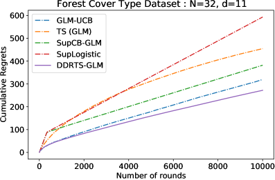
Figure 2: Comparison of the average cumulative regret on forest cover type dataset over 10 repeated runs.

We use the Forest Cover Type dataset from the UCI Machine Learning repository (Blake, Keogh, and Merz 1999), as used by Filippi et al. (2010). The dataset contains 581,021 observations, where the response variable is the label of the dominant species of trees of each region, and covariates include ten continuous cartographic variables characterizing features of the forest. We divide the dataset into $32$ clusters using the k-means clustering algorithm, and the resulting clusters of the forest represent arms. We repeat the experiment 10 times with $T=10,000$. Each centroid of each cluster is set to be a 10-dimensional context vector of the corresponding arm, and by introducing an intercept, we obtain $d=11$. In this example, context vectors remain unchanged in each round. We dichotomize the reward based on whether the forest’s dominant class is Spruce/Fir. The goal is to find arms with Spruce/Fir as the dominant class. We execute a 32-armed 11-dimensional contextual bandit with binary rewards. Figure 2 shows that DDRTS-GLM outperforms other algorithms.

Table 2: Average/first quartile/third quartile of CTR of news articles over 10 repeated runs for each algorithm.

CTR	1st Q	average	3rd Q
DDRTS-GLM	0.0410	0.0449	0.0476
GLM-UCB	0.0356	0.0420	0.0468
TS (GLM)	0.0393	0.0438	0.0467
uniform random	0.0337	0.0344	0.0351

6.3 Yahoo! news article recommendation log data

The Yahoo! Front Page Today Module User Click Log Dataset (Yahoo! Webscope 2009) contains 45,811,883 user click logs for news articles on Yahoo! Front Page from May 1st, 2009, to May 19th, 2009.Each log consists of a randomly chosen article from $N=20$ articles and the binary reward $Y_{t}$ which takes the value 1 if a user clicked the article and 0 otherwise. For each article $i\in[20]$, we have a context vector $X_{i,t}\in\mathbb{R}^{11}$ which comprising 10 extracted features of user-article information and an intercept using a dimension reduction method, as in Chu et al. (2009).

In log data, when the algorithm chooses an action not selected by the original logger, it cannot observe the reward, and the regret is not computable. Instead, we use the click-through rate (CTR): the percentage of the number of clicks. We tune the hyperparameters using the log data from May 1st and run the algorithms on the randomly sampled $10^{6}$ logs in each run. We evaluate the algorithms on the basis of the method by Li et al. (2011), counting only the rounds in which the reward is observed in $T$. Thus, $T$ is not known a priori and SupCB-GLM and SupLogistic are not applicable. As a baseline, we run a uniform random policy to observe the CTR lift of each algorithm. Table 2 presents the average/first quartile/third quartile of CTR of each algorithm (the higher is the better) over 10 repetitions, showing that DDRTS-GLM achieves the highest CTR.

Appendix A Generalized linear models

We consider a model in which the reward $Y$ is sampled from one-dimensional exponential family. When the reward is related to a context vector $X\in\mathbb{R}^{d}$, the GLM assumes that the probability density function of $Y$ is

$$\mathbb{P}\left(\left.Y=y\right|\theta\right)\propto\exp\left\{\theta y-b(\theta)\right\},$$

where $b$ represents a known function and $\theta\in\mathbb{R}$ is a canonical parameter related to both the reward and the context vector. When $b$ is twice differentiable, we have $b^{\prime}(\theta)=\text{$\mathbb{E}$}[Y]$, and $b^{\prime\prime}(\theta)=\mathbb{V}[Y]$. In the GLM, we assume that the expected value of $Y$ is related to context $X$ based on linear predictor, $\xi:=X^{T}\beta^{*}$ for some unknown parameter $\beta^{*}\in\mathbb{R}^{d}$. Then $\text{$\mathbb{E}$}[Y]:=\mu(\xi)$, with the inverse link function $\mu$. When $\theta=\xi$, the link function is called canonical link. Under a canonical link, $b^{\prime\prime}(\theta)\!=\!\mu^{\prime}(\xi)$. In the case of Bernoulli rewards, the inverse canonical link function is $\mu(\xi)\!=\!1/(1\!+\!\exp(-\xi))$. Throughout this study, we consider a canonical link case. An extension to non-canonical cases requires minor changes.

Let $(X_{1},Y_{1}),\ldots,(X_{t},Y_{t}$) be the independent pairs of contexts and rewards. Then, the log-likelihood function in a canonical link case is

$$\log l(\beta)=\sum_{\tau=1}^{t}\left\{Y_{\tau}X_{\tau}^{T}\beta-b\left(X_{\tau}^{T}\beta\right)\right\}+C\left(Y_{\tau}\right),$$

where $C(\cdot)$ is a function not related to $\beta$. Instead of minimizing $-\log l(\beta)$ to obtain an estimator, Segerstedt (1992) proposed adding $\frac{\lambda_{t}}{2}\beta^{T}\beta$ to $-\log l(\beta)$ for regularization. The regularization term plays a significant role in ensuring that the second derivative of $-\log l(\beta)$,

$$\sum_{\tau=1}^{t}b^{\prime\prime}\left(X_{\tau}^{T}\beta\right)X_{\tau}X_{\tau}^{T}+\lambda_{t}I,$$

has a sufficiently large positive eigenvalue. Since the objective function is strictly convex, we can obtain a ridge-type estimator by taking the derivative with respect to $\beta$ and solving $\sum_{\tau=1}^{t}\left\{Y_{\tau}X_{\tau}-\mu\left(X_{\tau}^{T}\beta\right)X_{\tau}\right\}-\lambda_{t}\beta=0.$ In practice, this equation can be solved using Newton’s algorithms.

Appendix B Comparison of the order of regret bounds for generalized/logistic bandits

In this section, we provide a table that compares the regret bounds for generalized/logistic bandit algorithms, with respect to $\kappa$, $d$, $N$ and $T$.

Table 3: Comparison of the main orders of the regret bounds for generalized/logistic bandit with respect to $\kappa,d,N$ and $T$.

Algorithm	Regret Upper Bound	Model
GLM-UCB (Filippi et al. 2010)	$O(\kappa^{-1}d\sqrt{T}\log^{3/2}T)$	GLM
SupCB-GLM (Li, Lu, and Zhou 2017)	$O(\kappa^{-1}\sqrt{dT\log NT}\log T$)	GLM
TS (GLM) (Abeille and Lazaric 2017)	$O(\kappa^{-1}d^{3/2}\sqrt{T}\log T)$	GLM
GLOC (Jun et al. 2017)	$O(\kappa^{-1}d\sqrt{T}\log^{3/2}T)$	GLM
GLOC-TS (Jun et al. 2017)	$\hat{\mathcal{O}}(\kappa^{-1}d^{3/2}\sqrt{T}\log^{3/2}T)$	GLM
Logistic UCB-1 (Faury et al. 2020)	$O(\kappa^{-1/2}d\sqrt{T}\log T)$	Logistic
Logistic-UCB-2 (Faury et al. 2020)	$O(d\sqrt{T}\log T)$	Logistic
SupLogistic (Jun et al. 2021)	$O(\sqrt{dT\log NT}\log T)$	Logistic
DDRTS-GLM (Proposed)	$O(\sqrt{\kappa^{-1}dT\log NT})$	GLM

Appendix C Detailed proofs for Theorem 5.1

In this section, we present the proof for the $\tilde{O}(\sqrt{\kappa^{-1}\phi T})$ regret bound for DDRTS-GLM and its related lemmas.

C.1 Proof of Lemma 5.4

Proof.

This proof is modified from that of Lemma 2 in Kim, Kim, and Paik (2021). Fix $t\in(\mathcal{T}_{*},T]$ and define $\Gamma_{t}:=\{i\in[N]:\tilde{\pi}_{i,t}>\gamma\}$ for given $\gamma\in[1/(N+1),1/N)$.

Step 1. Proving $\Gamma_{t}\subseteq S_{t}$:

By definition of $S_{t}$ in (5), we have $a_{t}^{*}\in S_{t}$. Let $\tilde{Y}_{i,t}:=\mu(X_{i,t}^{T}\tilde{\beta}_{i,t})$, where $\tilde{\beta}_{i,t}$ is the sampled from Gaussian distribution defined in Algorithm 1. Suppose the estimated reward for the optimal arm, $\tilde{Y}_{a_{t}^{*},t}$ is greater than $\tilde{Y}_{j,t}$ for all $j\in S_{t}$, i.e. $\max_{j\notin S_{t}}\tilde{Y}_{j,t}\leq\tilde{Y}_{a_{t}^{*},t}$. In this case, any arm $j\notin S_{t}$ cannot be selected as a candidate arm $\tilde{a}_{t}:=\arg\max_{i\in[N]}\tilde{Y}_{i,t}$ and $\tilde{a}_{t}\in S_{t}$. Thus,

$$\mathbb{P}\left(\left.\tilde{a}_{t}\in S_{t}\right|\mathcal{H}_{t}\right) \geq\mathbb{P}\left(\left.\bigcap_{j\notin S_{t}}\left\{\tilde{Y}_{a_{t}^{*},t}>\tilde{Y}_{j,t}\right\}\right|\mathcal{H}_{t}\right)$$

$$=\mathbb{P}\left(\left.\bigcap_{j\notin S_{t}}\left\{X_{a_{t}^{*},t}^{T}\tilde{\beta}_{a_{t}^{*},t}>X_{j,t}^{T}\tilde{\beta}_{j,t}\right\}\right|\mathcal{H}_{t}\right)$$

$$=\mathbb{P}\left(\left.\bigcap_{j\notin S_{t}}\left\{Z_{j,t}>\left(X_{j,t}-X_{a_{t}^{*},t}\right)^{T}\widehat{\beta}_{t-1}\right\}\right|\mathcal{H}_{t}\right),$$

where $Z_{j,t}:=X_{a_{t}^{*},t}^{T}\left(\tilde{\beta}_{a_{t}^{*},t}-\widehat{\beta}_{t-1}\right)-X_{j,t}^{T}\left(\tilde{\beta}_{j,t}-\widehat{\beta}_{t-1}\right)$. The first equality holds since $\mu$ is a nondecreasing function. Because the distribution of $\tilde{\beta}_{j,t}$ is Gaussian, we can deduce that $Z_{j,t}$ is a centered Gaussian random variable with variance $v^{2}(\|X_{a_{t}^{*},t}\|^{2}_{\widehat{W}_{t-1}^{-1}}+\|X_{j,t}\|_{\widehat{W}_{t-1}^{-1}}^{2})$, where $\widehat{W}_{t}:=\sum_{\tau=1}^{t}\sum_{i=1}^{N}\mu^{\prime}(X_{i,\tau}^{T}\widehat{\beta}_{t})X_{i,\tau}X_{i,\tau}^{T}+\lambda I_{d}$. Denote the inverse function of $\mu$ by $\mu^{-1}$. Then for each $j\notin S_{t}$, by mean value theorem, there exists $\bar{\mu}$ between $\mu(X_{a_{t}^{*},t}^{T}\widehat{\beta}_{t-1})$ and $\mu(X_{j,t}^{T}\widehat{\beta}_{t-1})$ such that

$$\left(X_{j,t}\!-\!X_{a_{t}^{*},t}\right)^{T}\!\!\widehat{\beta}_{t-1}\!\! =\!\left(\mu^{-1}\right)^{\prime}\!(\bar{\mu})\!\left\{\mu(X_{j,t}^{T}\widehat{\beta}_{t-1})-\mu(X_{a_{t}^{*},t}^{T}\widehat{\beta}_{t-1})\right\}$$

$$=\!\left(\mu^{-1}\right)^{\prime}\!(\bar{\mu})\!\left\{\!\mu(X_{j,t}^{T}\widehat{\beta}_{t-1})\!-\!\mu(X_{j,t}^{T}\beta^{*})\!-\!\mu(X_{a_{t}^{*},t}^{T}\widehat{\beta}_{t-1})\!+\!\mu(X_{a_{t}^{*},t}^{T}\beta^{*})\!-\!\Delta_{j}(t)\!\right\}$$

$$\leq\!\left(\mu^{-1}\right)^{\prime}\!(\bar{\mu})\!\left\{\mathcal{D}_{j}(t)+\mathcal{D}_{a_{t}^{*}}(t)-\Delta_{j}(t)\right\}$$

$$\leq\!\left(\mu^{-1}\right)^{\prime}\!(\bar{\mu})\!\left\{-\sqrt{\kappa L_{1}}\sqrt{\left\|X_{a_{t}^{*},t}\right\|_{W_{t-1}^{-1}}^{2}+\left\|X_{j,t}\right\|_{W_{t-1}^{-1}}^{2}}\right\}$$

$$\leq-\sqrt{\frac{\kappa}{L_{1}}}\sqrt{\left\|X_{a_{t}^{*},t}\right\|_{W_{t-1}^{-1}}^{2}+\left\|X_{j,t}\right\|_{W_{t-1}^{-1}}^{2}},$$

where the second inequality holds due to $j\notin S_{t}$ and (5), and the last inequality holds due to the fact that $(\mu^{-1})^{\prime}(y)=1/\mu^{\prime}(\mu^{-1}(y))\geq L_{1}^{-1}$ for all $y\in\{\mu(x^{T}\beta):\|x\|_{2}\leq 1,\beta\in\mathcal{B}_{r}^{*}\}$ (Assumption 3). By Assumption 3, and $\kappa\leq L_{1}$,

$$W_{t}:= \sum_{\tau=1}^{t}\sum_{i=1}^{N}\mu^{\prime}\left(X_{i,\tau}^{T}\beta^{*}\right)X_{i,\tau}X_{i,\tau}^{T}+\lambda I_{d}$$

$$\preceq L_{1}\sum_{\tau=1}^{t}\sum_{i=1}^{N}X_{i,\tau}X_{i,\tau}^{T}+\lambda I_{d}$$

$$\preceq \frac{L_{1}}{\kappa}\sum_{\tau=1}^{t}\sum_{i=1}^{N}\mu^{\prime}\left(X_{i,\tau}^{T}\widehat{\beta}_{t}\right)X_{i,\tau}X_{i,\tau}^{T}+\lambda I_{d}$$

$$\preceq \frac{L_{1}}{\kappa}\sum_{\tau=1}^{t}\sum_{i=1}^{N}\mu^{\prime}\left(X_{i,\tau}^{T}\widehat{\beta}_{t}\right)X_{i,\tau}X_{i,\tau}^{T}+\frac{L_{1}}{\kappa}\lambda I_{d}$$

$$= \frac{L_{1}}{\kappa}\widehat{W}_{t}.$$

This implies that for each $j\notin S_{t}$,

$$\left(X_{j,t}-X_{a_{t}^{*},t}\right)^{T}\widehat{\beta}_{t-1}\leq-\frac{\kappa}{L_{1}}\sqrt{\left\|X_{a_{t}^{*},t}\right\|_{\widehat{W}_{t-1}^{-1}}^{2}+\left\|X_{j,t}\right\|_{\widehat{W}_{t-1}^{-1}}^{2}}.$$ (14)

Thus, we have

$$\mathbb{P}\left(\left.\tilde{a}_{t}\in S_{t}\right|\mathcal{H}_{t}\right)\geq \mathbb{P}\left(\left.\bigcap_{j\notin S_{t}}\left\{Z_{j,t}>-\frac{\kappa}{L_{1}}\sqrt{\left\|X_{a_{t}^{*},t}\right\|_{\widehat{W}_{t-1}^{-1}}^{2}+\left\|X_{j,t}\right\|_{\widehat{W}_{t-1}^{-1}}^{2}}\right\}\right|\mathcal{H}_{t}\right)$$

$$= \mathbb{P}\left(\left.\bigcap_{j\notin S_{t}}\left\{\frac{Z_{j,t}}{v\sqrt{\left\|X_{a_{t}^{*},t}\right\|_{\widehat{W}_{t-1}^{-1}}^{2}+\left\|X_{j,t}\right\|_{\widehat{W}_{t-1}^{-1}}^{2}}}>-\frac{\kappa}{L_{1}}v^{-1}\right\}\right|\mathcal{H}_{t}\right)$$

$$:= \mathbb{P}\left(\left.\bigcap_{j\notin S_{t}}\left\{U_{j,t}>-\frac{\kappa}{L_{1}}v^{-1}\right\}\right|\mathcal{H}_{t}\right).$$

Here, $\{U_{j,t}\}_{j\notin S_{t}}$ are independent standard Gaussian random variables given $\mathcal{H}_{t}$. Setting $v=(\kappa/L_{1})\left\{2\log\left(\frac{N}{1-\gamma N}\right)\right\}^{-1/2}$ gives

$$\mathbb{P}\left(\left.U_{j,t}<-\frac{\kappa}{L_{1}}v^{-1}\right|\mathcal{H}_{t}\right)\leq\frac{1-\gamma N}{N},$$

for each $j\notin S_{t}$. Then we have

$$\mathbb{P}\left(\left.\bigcap_{j\notin S_{t}}\left\{U_{j,t}>-\frac{\kappa}{L_{1}}v^{-1}\right\}\right|\mathcal{H}_{t}\right)= \prod_{j\notin S_{t}}\mathbb{P}\left(\left.U_{j,t}>-\frac{\kappa}{L_{1}}v^{-1}\right|\mathcal{H}_{t}\right)$$

$$= \prod_{j\notin S_{t}}\left\{1-\mathbb{P}\left(\left.U_{j,t}<-\frac{\kappa}{L_{1}}v^{-1}\right|\mathcal{H}_{t}\right)\right\}$$

$$\geq \prod_{j\notin S_{t}}\left\{1-\frac{1-\gamma N}{N}\right\}$$

$$\geq 1-\left(1-\gamma N\right)$$

$$= \gamma N$$

$$\geq 1-\gamma,$$

where the last inequality holds due to $\gamma>1/(N+1)$. With (14), we have $\mathbb{P}\left(\left.\tilde{a}_{t}\in S_{t}\right|\mathcal{H}_{t}\right)\geq 1-\gamma$. For any $j\notin S_{t}$,

$$\tilde{\pi}_{j,t}=\mathbb{P}\left(\left.\tilde{a}_{t}=j\right|\mathcal{H}_{t}\right)\leq\mathbb{P}\left(\left.\bigcup_{j\notin S_{t}}\left\{\tilde{a}_{t}=j\right\}\right|\mathcal{H}_{t}\right)=\mathbb{P}\left(\left.\tilde{a}_{t}\notin S_{t}\right|\mathcal{H}_{t}\right)\leq\gamma.$$

Thus, we conclude that $S_{t}^{c}\subseteq\Gamma_{t}^{c}$.

Step 2. Proving $a_{t}\in\Gamma_{t}$ with high probability:

For $m\in[M_{t}]$, let $a_{t}^{(m)}$ be the candidate arm in $m$-th resampling. Since $a_{t}^{(1)},\ldots,a_{t}^{(M_{t})}$ are independent,

$$\mathbb{P}\left(\left.a_{t}\notin\Gamma_{t}\right|\mathcal{H}_{t}\right)\leq\mathbb{P}\left(\left.\bigcap_{m=1}^{M_{t}}\left\{a_{t}^{(m)}\notin\Gamma_{t}\right\}\right|\mathcal{H}_{t}\right)=\prod_{m=1}^{M_{t}}\mathbb{P}\left(\left.a_{t}^{(m)}\notin\Gamma_{t}\right|\mathcal{H}_{t}\right)\leq\left(1-\gamma\right)^{M_{t}},$$

where the last inequality holds because $\gamma<1/N$ and there exists at least one arm $i$ such that $\tilde{\pi}_{i,t}>\gamma$, which implies $\mathbb{P}\left(\left.a_{t}^{(m)}\notin\Gamma_{t}\right|\mathcal{H}_{t}\right)\leq 1-\gamma$. Setting $M_{t}=\log\frac{(t+1)^{2}}{\delta}\Big{/}\log\frac{1}{1-\gamma}$ proves

$$\mathbb{P}\left(\left.a_{t}\in\Gamma_{t}\right|\mathcal{H}_{t}\right)\geq 1-\frac{\delta}{t^{2}},$$

for all $t\in[T]$.

Step 3. Proving the lemma:

Because $\Gamma_{t}\subseteq S_{t}$ for $t\in(\mathcal{T}_{*},T]$, we can deduce that $a_{t}\in\Gamma_{t}$ implies $a_{t}\in S_{t}$. Because $\pi_{i,t}\geq\tilde{\pi}_{i,t}$ for all $i\in\Gamma_{t}$ and $t\in[T]$, we have that $a_{t}\in\Gamma_{t}$ implies $\pi_{a_{t},t}>\gamma$. Thus, we conclude that

$$\mathbb{P}\left(\bigcap_{t=\mathcal{T}_{*}}^{T}\left\{a_{t}\in S_{t}\right\}\cap\bigcap_{t=1}^{T}\left\{\pi_{a_{t},t}>\gamma\right\}\right)\geq\mathbb{P}\left(\bigcap_{t=1}^{T}\left\{a_{t}\in\Gamma_{t}\right\}\right)\geq 1-\delta$$

∎

C.2 Proof of Lemma 5.6

Proof.

Let us fix $t\in(\mathcal{T}_{*},T]$. Then the tail inequality for DDR estimator (Theorem E.3) and Corollary F.2 imply that, with probability at least $1-6\delta/T$,

$$\begin{split}\left\|\widehat{\beta}_{t-1}-\beta^{*}\right\|_{2}&\leq\frac{12L_{1}+8B}{\kappa\phi\sqrt{t-1}}\sqrt{\log\frac{4T}{\delta}}+\frac{\frac{9}{4}L_{1}r+\frac{\lambda S}{N}}{\kappa\phi\left(t-1\right)},\\ \min_{\beta\in\mathcal{B}_{r}^{*}}\lambda_{\text{min}}\left(\sum_{\tau=1}^{t-1}\sum_{i=1}^{N}\mu^{\prime}\left(X_{i,\tau}^{T}\beta\right)X_{i,\tau}X_{i,\tau}^{T}\right)&\geq\frac{\phi\kappa N\left(t-1\right)}{2}.\end{split}$$ (15)

As the second line of event is required for the first line of event, (15) holds with probability at least $1-6\delta$ not $1-7\delta$.

Step 1 Approximation:

For each $j\in[N]$, using second-order Taylor expansion, there exists $v\in(0,1)$ such that $\bar{\beta}=v\widehat{\beta}_{t-1}+(1-v)\beta^{*}$ and

$$\mu\left(X_{j,t}^{T}\widehat{\beta}_{t-1}\right)-\mu\left(X_{j,t}^{T}\beta^{*}\right)=\mu^{\prime}\left(X_{j,t}^{T}\beta^{*}\right)X_{j,t}^{T}\left(\widehat{\beta}_{t-1}-\beta^{*}\right)+\frac{\mu^{\prime\prime}\left(X_{j,t}^{T}\bar{\beta}\right)\left\{X_{j,t}^{T}\left(\widehat{\beta}_{t-1}-\beta^{*}\right)\right\}^{2}}{2}.$$

Taking the absolute value on both sides,

$$\begin{split}\left|\mu\left(X_{j,t}^{T}\widehat{\beta}_{t-1}\right)-\mu\left(X_{j,t}^{T}\beta^{*}\right)\right|\leq&\left|\mu^{\prime}\left(X_{j,t}^{T}\beta^{*}\right)X_{j,t}^{T}\left(\widehat{\beta}_{t-1}-\beta^{*}\right)\right|\\ &\;+\left|\frac{\mu^{\prime\prime}\left(X_{j,t}^{T}\bar{\beta}\right)\left\{X_{j,t}^{T}\left(\widehat{\beta}_{t-1}-\beta^{*}\right)\right\}^{2}}{2}\right|\\ \leq&\mu^{\prime}\left(X_{j,t}^{T}\beta^{*}\right)\left|X_{j,t}^{T}\left(\widehat{\beta}_{t-1}-\beta^{*}\right)\right|+\frac{L_{2}\left\|\widehat{\beta}_{t-1}-\beta\right\|_{2}^{2}}{2}\\ \leq&\mu^{\prime}\left(X_{j,t}^{T}\beta^{*}\right)\left|X_{j,t}^{T}\left(\widehat{\beta}_{t-1}-\beta^{*}\right)\right|\\ &+L_{2}\left\{\frac{\left(12L_{1}+8B\right)^{2}}{\kappa^{2}\phi^{2}\left(t-1\right)}\log\frac{4T}{\delta}+\frac{\left(\frac{9}{4}L_{1}r+\frac{\lambda S}{N}\right)^{2}}{\kappa^{2}\phi^{2}N^{2}\left(t-1\right)^{2}}\right\}\\ \leq&\mu^{\prime}\left(X_{j,t}^{T}\beta^{*}\right)\left|X_{j,t}^{T}\left(\widehat{\beta}_{t-1}-\beta^{*}\right)\right|\\ &\;+\frac{L_{2}\left\{\left(12L_{1}+8B\right)^{2}+1\right\}}{\phi^{2}\kappa^{2}\left(t-1\right)}\log\frac{4T}{\delta}.\end{split}$$ (16)

The second inequality holds due to Assumption 1 and 3, and the third inequality holds by (15). The last inequality uses the fact that $t>\mathcal{T}_{*}$ and

$$\frac{\left(\frac{9}{4}L_{1}r+\frac{\lambda S}{N}\right)^{2}}{\kappa^{2}\phi^{2}\left(t-1\right)^{2}}\leq\frac{\left(\frac{9}{4}L_{1}r+\frac{\lambda S}{N}\right)^{2}}{\kappa^{2}\phi^{2}\left(t-1\right)\mathcal{T}_{*}}\leq\frac{1}{\phi^{2}\kappa^{2}\left(t-1\right)}\log\frac{4T}{\delta}.$$

To bound the first term in (16), we observe that $U_{t-1}(\widehat{\beta}_{t-1})=0$, where $U_{t}$ is the score function defined in (3). Let $W_{t}:=\sum_{\tau=1}^{t}\sum_{i=1}^{N}\mu^{\prime}\left(X_{i,\tau}^{T}\beta^{*}\right)X_{i,\tau}X_{i,\tau}^{T}+\lambda I_{d}$. Then by second-order Taylor expansion, there exists $v\in(0,1)$ such that $\bar{\beta}=v\widehat{\beta}_{t-1}+(1-v)\beta^{*}$ and

$$0 =U_{t-1}\left(\widehat{\beta}_{t-1}\right)$$

$$=U_{t-1}\left(\beta^{*}\right)-W_{t-1}\left(\widehat{\beta}_{t-1}-\beta^{*}\right)-\frac{1}{2}\sum_{\tau=1}^{t-1}\sum_{i=1}^{N}\mu^{\prime\prime}\left(X_{i,\tau}^{T}\bar{\beta}\right)\left\{X_{i,\tau}^{T}\left(\widehat{\beta}_{t-1}-\beta^{*}\right)\right\}^{2}X_{i,\tau}.$$

Multiplying $X_{j,t}^{T}W_{t-1}^{-1}$ on both sides gives

$$X_{j,t}^{T}\left(\widehat{\beta}_{t-1}-\beta^{*}\right) =X_{j,t}^{T}W_{t-1}^{-1}U_{t-1}\left(\beta^{*}\right)$$

$$\quad-\frac{1}{2}\sum_{\tau=1}^{t-1}\sum_{i=1}^{N}\mu^{\prime\prime}\left(X_{i,\tau}^{T}\bar{\beta}\right)\left\{X_{i,\tau}^{T}\left(\widehat{\beta}_{t-1}-\beta^{*}\right)\right\}^{2}X_{j,t}^{T}W_{t-1}^{-1}X_{i,\tau}.$$

Taking the absolute value on both sides,

$$\begin{split}\left|X_{j,t}^{T}\left(\widehat{\beta}_{t-1}-\beta^{*}\right)\right|\leq&\left|X_{j,t}^{T}W_{t-1}^{-1}U_{t-1}\left(\beta^{*}\right)\right|\\ &\quad+\frac{1}{2}\left|\sum_{\tau=1}^{t-1}\sum_{i=1}^{N}\mu^{\prime\prime}\left(X_{i,\tau}^{T}\bar{\beta}\right)\left\{X_{i,\tau}^{T}\left(\widehat{\beta}_{t-1}-\beta^{*}\right)\right\}^{2}X_{j,t}^{T}W_{t-1}^{-1}X_{i,\tau}\right|\\ \leq&\left|X_{j,t}^{T}W_{t-1}^{-1}U_{t-1}\left(\beta^{*}\right)\right|+\frac{L_{2}\left\|\widehat{\beta}_{t-1}-\beta^{*}\right\|_{2}^{2}}{2}\sum_{\tau=1}^{t-1}\sum_{i=1}^{N}\left|X_{j,t}^{T}W_{t-1}^{-1}X_{i,\tau}\right|\\ \leq&\left|X_{j,t}^{T}W_{t-1}^{-1}U_{t-1}\left(\beta^{*}\right)\right|+\frac{L_{2}\left\|\widehat{\beta}_{t-1}-\beta^{*}\right\|_{2}^{2}\lambda_{\text{min}}\left(W_{t-1}\right)^{-1}N\left(t-1\right)}{2}\\ \leq&\left|X_{j,t}^{T}W_{t-1}^{-1}U_{t-1}\left(\beta^{*}\right)\right|+\frac{L_{2}}{\phi\kappa}\left\{\frac{\left(12L_{1}+8B\right)^{2}}{\phi^{2}\kappa^{2}\left(t-1\right)}\log\frac{4T}{\delta}+\frac{\left(\frac{9}{4}L_{1}r+\frac{\lambda S}{N}\right)^{2}}{\kappa^{2}\phi^{2}(t-1)^{2}}\right\}\\ \leq&\left|X_{j,t}^{T}W_{t-1}^{-1}U_{t-1}\left(\beta^{*}\right)\right|+\frac{L_{2}\left\{\left(12L_{1}+8B\right)^{2}+1\right\}}{\phi^{3}\kappa^{3}\left(t-1\right)}\log\frac{4T}{\delta}.\end{split}$$ (17)

The second and third inequality holds due to Assumption 1 and 3, and the fourth inequality holds due to (15). By Assumption 1 and (15),

$$\begin{split}\left|X_{j,t}^{T}W_{t-1}^{-1}U_{t-1}\left(\beta^{*}\right)\right|=&\left|X_{j,t}^{T}W_{t-1}^{-1}\left[\sum_{\tau=1}^{t-1}\sum_{i=1}^{N}\left\{Y_{i,\tau}^{\breve{\beta}_{t-1}}-\mu\left(X_{i,\tau}^{T}\beta^{*}\right)\right\}X_{i,\tau}-\lambda\beta^{*}\right]\right|\\ \leq&\left|\sum_{\tau=1}^{t-1}\sum_{i=1}^{N}\left\{Y_{i,\tau}^{\breve{\beta}_{t-1}}-\mu\left(X_{i,\tau}^{T}\beta^{*}\right)\right\}X_{j,t}^{T}W_{t-1}^{-1}X_{i,\tau}\right|+\lambda\left|X_{j,t}^{T}W_{t-1}^{-1}\beta^{*}\right|\\ \leq&\left|\sum_{\tau=1}^{t-1}\sum_{i=1}^{N}\left\{Y_{i,\tau}^{\breve{\beta}_{t-1}}-\mu\left(X_{i,\tau}^{T}\beta^{*}\right)\right\}X_{j,t}^{T}W_{t-1}^{-1}X_{i,\tau}\right|+\lambda S\lambda_{\text{min}}\left(W_{t-1}\right)^{-1}\\ =&\left|\sum_{\tau=1}^{t-1}\sum_{i=1}^{N}\left\{Y_{i,\tau}^{\breve{\beta}_{t-1}}-\mu\left(X_{i,\tau}^{T}\beta^{*}\right)\right\}X_{j,t}^{T}W_{t-1}^{-1}X_{i,\tau}\right|+\frac{2\lambda S}{\kappa\phi N\left(t-1\right)}.\end{split}$$ (18)

From (16), (17) and (18), the bound for the prediction error is approximated by

$$\mathcal{D}_{j}(t)\leq\mu^{\prime}\left(X_{j,t}^{T}\beta^{*}\right)\left|\sum_{\tau=1}^{t-1}\sum_{i=1}^{N}\left\{Y_{i,\tau}^{\breve{\beta}_{t-1}}-\mu\left(X_{i,\tau}^{T}\beta^{*}\right)\right\}X_{j,t}^{T}W_{t-1}^{-1}X_{i,\tau}\right|+\frac{D_{\mu,B,\lambda,S}-3L_{1}}{\phi^{3}\kappa^{3}\left(t-1\right)}\log\frac{4T}{\delta},$$ (19)

where

$$D_{\mu,B,\lambda,S}:=2L_{2}\left\{\left(12L_{1}+8B\right)^{2}+1\right\}+2\lambda S+3L_{1}.$$ (20)

Step 2 Bounding the main order term:

Now we bound the first term in (19), which is the main order term. By definition of $Y_{i,\tau}^{\breve{\beta}_{t-1}}$,

$$\begin{split}&\left|\sum_{\tau=1}^{t-1}\sum_{i=1}^{N}\left\{Y_{i,\tau}^{\breve{\beta}_{t-1}}-\mu\left(X_{i,\tau}^{T}\beta^{*}\right)\right\}X_{j,t}^{T}W_{t-1}^{-1}X_{i,\tau}\right|\\ &\leq\left|\sum_{\tau=1}^{t-1}\sum_{i=1}^{N}\left\{1-\frac{\mathbb{I}\left(a_{\tau}=i\right)}{\pi_{i,\tau}}\right\}D_{i,\tau}^{\breve{\beta}_{t-1}}X_{j,t}^{T}W_{t-1}^{-1}X_{i,\tau}\right|+\left|\sum_{\tau=1}^{t-1}\frac{\eta_{\tau}}{\pi_{a_{\tau},\tau}}X_{j,t}^{T}W_{t-1}^{-1}X_{a_{\tau},\tau}\right|.\end{split}$$ (21)

where $D_{i,\tau}^{\breve{\beta}_{t}}:=\mu(X_{i,\tau}^{T}\breve{\beta}_{t})-\mu(X_{i,\tau}^{T}\beta^{*})$, and $\eta_{\tau}:=Y_{\tau}-\mu(X_{a_{\tau},\tau}^{T}\beta^{*})$. To bound the first term, we let $A_{i,\tau}:=1-\frac{\mathbb{I}\left(a_{\tau}=i\right)}{\pi_{i,\tau}}$ and define $\breve{\mathcal{B}}:=\{\beta\in\mathbb{R}^{d}:\|\beta-\beta^{*}\|_{2}\leq\min\{\kappa^{1/2}N^{-1/2}d^{-1/2},r\}\}$. By Lemma E.2, the imputation estimator $\breve{\beta}_{t}$ is in $\breve{\mathcal{B}}$, with probability at least $1-3\delta/T$. For any $\epsilon>0$, let $\beta_{1},\ldots,\beta_{M(\epsilon)}$ be the $\epsilon$-cover for $\breve{\mathcal{B}}$. Then for any $\beta\in\breve{\mathcal{B}}$, there exists $m\in[M(\epsilon)]$ such that $\|\beta-\beta_{m}\|_{2}\leq\epsilon$ and

$$\left|\sum_{\tau=1}^{t-1}\sum_{i=1}^{N}A_{i,\tau}D_{i,\tau}^{\beta}X_{j,t}^{T}W_{t-1}^{-1}X_{i,\tau}\right|$$

$$\leq\left|\sum_{\tau=1}^{t-1}\sum_{i=1}^{N}A_{i,\tau}\left(D_{i,\tau}^{\beta}-D_{i,\tau}^{\beta_{m}}\right)X_{j,t}^{T}W_{t-1}^{-1}X_{i,\tau}\right|+\left|\sum_{\tau=1}^{t-1}\sum_{i=1}^{N}A_{i,\tau}D_{i,\tau}^{\beta_{m}}X_{j,t}^{T}W_{t-1}^{-1}X_{i,\tau}\right|$$

$$\leq L_{1}\epsilon\sum_{\tau=1}^{t-1}\sum_{i=1}^{N}\left|A_{i,\tau}X_{j,t}^{T}W_{t-1}^{-1}X_{i,\tau}\right|+\max_{m\in[M(\epsilon)]}\left|\sum_{\tau=1}^{t-1}\sum_{i=1}^{N}A_{i,\tau}D_{i,\tau}^{\beta_{m}}X_{j,t}^{T}W_{t-1}^{-1}X_{i,\tau}\right|$$

$$\leq L_{1}\epsilon\lambda_{\text{min}}\left(W_{t-1}\right)^{-1}\sum_{\tau=1}^{t-1}\sum_{i=1}^{N}\left|A_{i,\tau}\right|+\max_{m\in[M(\epsilon)]}\left|\sum_{\tau=1}^{t-1}\sum_{i=1}^{N}A_{i,\tau}D_{i,\tau}^{\beta_{m}}X_{j,t}^{T}W_{t-1}^{-1}X_{i,\tau}\right|$$

$$\leq\frac{2L_{1}\epsilon\left(\gamma^{-1}+N\right)}{\kappa\phi N}+\max_{m\in[M(\epsilon)]}\left|\sum_{\tau=1}^{t-1}\sum_{i=1}^{N}A_{i,\tau}D_{i,\tau}^{\beta_{m}}X_{j,t}^{T}W_{t-1}^{-1}X_{i,\tau}\right|.$$

The second inequality holds due to Assumption 1 and 3, the third inequality holds by Assumption 1 and the last inequality holds by (15) and the event in (6). Taking the supremum over $\breve{\mathcal{B}}$ gives

$$\begin{split}&\left|\sum_{\tau=1}^{t-1}\sum_{i=1}^{N}A_{i,\tau}D_{i,\tau}^{\breve{\beta}_{t-1}}X_{j,t}^{T}W_{t-1}^{-1}X_{i,\tau}\right|\\ &\leq\sup_{\beta\in\breve{\mathcal{B}}}\left|\sum_{\tau=1}^{t-1}\sum_{i=1}^{N}A_{i,\tau}D_{i,\tau}^{\beta}X_{j,t}^{T}W_{t-1}^{-1}X_{i,\tau}\right|\\ &\leq\frac{2L_{1}\epsilon\left(\gamma^{-1}+N\right)}{\kappa\phi N}+\max_{m\in[M(\epsilon)]}\left|\sum_{\tau=1}^{t-1}\sum_{i=1}^{N}A_{i,\tau}D_{i,\tau}^{\beta_{m}}X_{j,t}^{T}W_{t-1}^{-1}X_{i,\tau}\right|\\ &\leq\frac{6L_{1}\epsilon}{\kappa\phi}+\max_{m\in[M(\epsilon)]}\left|\sum_{\tau=1}^{t-1}\sum_{i=1}^{N}A_{i,\tau}D_{i,\tau}^{\beta_{m}}X_{j,t}^{T}W_{t-1}^{-1}X_{i,\tau}\right|,\end{split}$$ (22)

where the last inequality holds due to $\gamma>1/(N+1)$. Define the filtration $\mathcal{F}_{\tau}:=\mathcal{H}_{\tau}\cup\{\mathcal{X}_{1},\ldots,\mathcal{X}_{t}\}$, and $\mathcal{F}_{0}=\{\mathcal{X}_{1},\ldots,\mathcal{X}_{t}\}$. Then for each $m\in[M(\epsilon)]$, let

$$P_{u}^{(m)}:=\sum_{\tau=1}^{u}\sum_{i=1}^{N}A_{i,\tau}D_{i,\tau}^{\beta_{m}}X_{j,t}^{T}W_{t-1}^{-1}X_{i,\tau},\quad P_{0}^{(m)}=0.$$

Then $P_{u}^{(m)}$ is a martingale sequence with respect to $\mathcal{F}_{u}$ because $P_{u}^{(m)}$ is $\mathcal{F}_{u+1}$-measurable, and

$$\text{$\mathbb{E}$}\left[\left.P_{u}^{(m)}\right|\mathcal{F}_{s}\right]= P_{u-1}^{(m)}+\text{$\mathbb{E}$}\left[\left.\sum_{i=1}^{N}A_{i,u}D_{i,u}^{\beta_{m}}X_{j,t}^{T}W_{t-1}^{-1}X_{i,u}\right|\mathcal{F}_{u}\right]$$

$$= P_{u-1}^{(m)}+\text{$\mathbb{E}$}\left[\left.\sum_{i=1}^{N}A_{i,u}\right|\mathcal{F}_{u}\right]D_{i,u}^{\beta_{m}}X_{j,t}^{T}W_{t-1}^{-1}X_{i,u}$$

$$= P_{u-1}^{(m)}+\text{$\mathbb{E}$}\left[\left.\sum_{i=1}^{N}A_{i,u}\right|\mathcal{H}_{u}\right]D_{i,u}^{\beta_{m}}X_{j,t}^{T}W_{t-1}^{-1}X_{i,u}$$

$$= P_{u-1}^{(m)}$$

where the third inequality holds since $\mathcal{H}_{u}$ is independent with $\mathcal{X}_{u+1},\ldots,\mathcal{X}_{t}$ because of Assumption 4. Let

$$E_{\gamma}:=\bigcap_{t=\mathcal{T}_{*}}^{T}\left\{a_{t}\in S_{t}\right\}\cap\bigcap_{t=1}^{T}\left\{\pi_{a_{t},t}>\gamma\right\}$$

When $E_{\gamma}$ holds, the differences of the martingale is bounded as

$$\left|P_{u}^{(m)}-P_{u-1}^{(m)}\right|= \left|\sum_{i=1}^{N}A_{i,u}D_{i,u}^{\beta_{m}}X_{i,t}^{T}W_{t-1}^{-1}X_{i,u}\right|$$

$$\leq \sqrt{\sum_{i=1}^{N}A_{i,u}^{2}}\sqrt{\sum_{i=1}^{N}\left(D_{i,u}^{\beta_{m}}X_{i,t}^{T}W_{t-1}^{-1}X_{i,u}\right)^{2}}$$

$$\leq \sqrt{N+\pi_{a_{u},u}^{-2}}L_{1}\left\|\beta_{m}-\beta^{*}\right\|_{2}\sqrt{\sum_{i=1}^{N}\left(X_{i,t}^{T}W_{t-1}^{-1}X_{i,u}\right)^{2}}$$

$$\leq \sqrt{N+\gamma^{-2}}L_{1}\left\|\beta_{m}-\beta^{*}\right\|_{2}\sqrt{\sum_{i=1}^{N}\left(X_{i,t}^{T}W_{t-1}^{-1}X_{i,u}\right)^{2}}$$

$$\leq 2L_{1}\sqrt{1+\gamma^{-2}N^{-1}}\sqrt{\frac{\kappa}{d}\sum_{i=1}^{N}\left(X_{i,t}^{T}W_{t-1}^{-1}X_{i,u}\right)^{2}}$$

$$\leq 2L_{1}\sqrt{\frac{3\kappa N}{d}\sum_{i=1}^{N}\left(X_{i,t}^{T}W_{t-1}^{-1}X_{i,u}\right)^{2}},$$

for all $u\in[t-1]$, and $m\in[M(\epsilon)]$. The fourth inequality holds since $\beta_{m}\in\breve{\mathcal{B}}$, and the last inequality holds since $\gamma\in[1/(N+1),1/N)$. Thus we have

$$\left\{\left|P_{u}^{(m)}-P_{u-1}^{(m)}\right|>2L_{1}\sqrt{\frac{3N\kappa}{d}\sum_{i=1}^{N}\left(X_{i,t}^{T}W_{t-1}^{-1}X_{i,u}\right)^{2}}\right\}\subset E_{\gamma}^{c}.$$

By Lemma G.1, there exists a martingale sequence $Q_{u}^{(m)}$ such that

$$\left|Q_{u}^{(m)}-Q_{u-1}^{(m)}\right|\leq 2L_{1}\sqrt{\frac{3N\kappa}{d}\sum_{i=1}^{N}\left(X_{i,t}^{T}W_{t-1}^{-1}X_{i,u}\right)^{2}},$$

almost surely, and

$$\left\{Q_{u}^{(m)}\neq P_{u}^{(m)}\right\}\subset\left\{\left|P_{u}^{(m)}-P_{u-1}^{(m)}\right|>2L_{1}\sqrt{\frac{3N\kappa}{d}\sum_{i=1}^{N}\left(X_{i,t}^{T}W_{t-1}^{-1}X_{i,u}\right)^{2}}\right\}\subset E_{\gamma}^{c},$$

for all $u\in[t-1]$. By Lemma G.4, for any $a>0$,

$$\mathbb{P}\left(\left.\left\{\max_{m\in[M(\epsilon)]}\left|P_{t-1}^{(m)}\right|>a\right\}\cap E_{\gamma}\right|\mathcal{F}_{0}\right)$$

$$\leq\mathbb{P}\left(\left.\max_{m\in[M(\epsilon)]}\left|Q_{t-1}^{(m)}\right|>a\right|\mathcal{F}_{0}\right)$$

$$\leq\sum_{m=1}^{M(\epsilon)}\mathbb{P}\left(\left.\left|Q_{t-1}^{(m)}\right|>a\right|\mathcal{F}_{0}\right)$$

$$\leq 2M(\epsilon)\exp\left(-\frac{da^{2}}{24L_{1}^{2}N\kappa\sum_{\tau=1}^{t-1}\sum_{i=1}^{N}\left(X_{j,t}^{T}W_{t-1}^{-1}X_{i,\tau}\right)^{2}}\right)$$

$$\leq 2M(\epsilon)\exp\left(-\frac{da^{2}}{24NL_{1}^{2}\left\|X_{j,t}\right\|_{W_{t-1}^{-1}}^{2}}\right),$$

where the last inequality holds because

$$\begin{split}\kappa\sum_{\tau=1}^{t-1}\sum_{i=1}^{N}\left(X_{j,t}^{T}W_{t-1}^{-1}X_{i,\tau}\right)^{2}&\leq X_{j,t}^{T}W_{t-1}^{-1}\left(\sum_{\tau=1}^{t-1}\mu^{\prime}\left(X_{i,\tau}^{T}\beta^{*}\right)X_{i,\tau}X_{i,\tau}^{T}\right)W_{t-1}^{-1}X_{j,t}\\ &\leq X_{j,t}^{T}W_{t-1}^{-1}X_{j,t}.\end{split}$$ (23)

Thus, with (22) and the event $E_{\gamma}$, with probability at least $1-\delta/(NT)$,

$$\left|\sum_{\tau=1}^{t-1}\sum_{i=1}^{N}A_{i,\tau}D_{i,\tau}^{\breve{\beta}_{t-1}}X_{j,t}^{T}W_{t-1}^{-1}X_{i,\tau}\right|\leq \frac{6L_{1}\epsilon}{\kappa\phi}+\max_{m\in[M(\epsilon)]}\left|\sum_{\tau=1}^{t-1}\sum_{i=1}^{N}A_{i,\tau}D_{i,\tau}^{\beta_{m}}X_{j,t}^{T}W_{t-1}^{-1}X_{i,\tau}\right|$$

$$\leq \frac{6L_{1}\epsilon}{\kappa\phi}+L_{1}\left\|X_{j,t}\right\|_{W_{t-1}^{-1}}\sqrt{\frac{24N}{d}\log\frac{2M(\epsilon)NT}{\delta}}.$$

Since the radius of $\breve{\mathcal{B}}$ is $\min\{\kappa^{1/2}N^{-1/2}d^{-1/2},r\}$, we have a bound for the covering number $M(\epsilon)$ by

$$M(\epsilon)\leq\left(\frac{2}{\epsilon}\min\left\{\sqrt{\frac{\kappa}{Nd}},r\right\}+1\right)^{d}\leq\left(\frac{3\sqrt{\kappa}}{\sqrt{Nd}\epsilon}\right)^{d}.$$

Setting $\epsilon=\frac{3\sqrt{\kappa}}{t-1}\frac{1}{N\sqrt{Nd}}$ gives

$$M(\epsilon)\leq\left\{N\left(t-1\right)\right\}^{d}\leq\left(NT\right)^{d},$$

and we obtain a following bound for the first term in (19):

$$\left|\sum_{\tau=1}^{t-1}\sum_{i=1}^{N}A_{i,\tau}D_{i,\tau}^{\breve{\beta}_{t-1}}X_{j,t}^{T}W_{t-1}^{-1}X_{i,\tau}\right|\leq\frac{3}{\sqrt{\kappa}\phi N\sqrt{N}\left(t-1\right)}+4L_{1}\left\|X_{j,t}\right\|_{W_{t-1}^{-1}}\sqrt{3N\log\frac{2NT}{\delta}}.$$ (24)

To bound the second term in (19), let

$$P_{u}:=\sum_{\tau=1}^{u}\frac{\eta_{\tau}\mathbb{I}\left(\pi_{a_{\tau},\tau}>\gamma\right)}{\pi_{a_{\tau},\tau}}X_{j,t}^{T}W_{t-1}^{-1}X_{a_{\tau},\tau},\quad P_{0}=0.$$

Then $P_{u}$ is a martingale sequence with respect to the filtration $\mathcal{F}_{u}:=\mathcal{H}_{u}\cup\{\mathcal{X}_{1},\ldots,\mathcal{X}_{t}\}$ and $\mathcal{F}_{0}:=\{\mathcal{X}_{1},\ldots,\mathcal{X}_{t}\}$ whose differences are bounded by

$$\left|\Delta P_{u}\right|:=\left|P_{u}-P_{u-1}\right|\leq \left|\frac{\eta_{u}\mathbb{I}\left(\pi_{a_{u},u}>\gamma\right)}{\pi_{a_{u},u}}X_{j,t}^{T}W_{t-1}^{-1}X_{a_{u},u}\right|$$

$$\leq \frac{2B}{\gamma}\left|X_{j,t}^{T}W_{t-1}^{-1}X_{a_{u},u}\right|$$

$$\leq \frac{2B}{\gamma}\left\|X_{j,t}\right\|_{W_{t-1}^{-1}}\lambda_{\text{min}}\left(W_{t-1}\right)^{-1/2}$$

almost surely. Since $W_{t-1}$ is $\mathcal{F}_{0}$-measurable, we can further bound the difference under the $\mathcal{F}_{0}$-measurable event (15) by

$$\left|\Delta P_{u}\right|\leq\frac{2B}{\gamma}\left\|X_{j,t}\right\|_{W_{t-1}^{-1}}\lambda_{\text{min}}\left(W_{t-1}\right)^{-1/2}\leq\frac{2B}{\gamma\sqrt{\kappa\phi N(t-1)}}\left\|X_{j,t}\right\|_{W_{t-1}^{-1}}.$$

The sum of conditional variances is bounded by,

$$\mathcal{V}_{t-1}:=\sum_{\tau=1}^{t-1}\text{$\mathbb{E}$}\left[\left.\left(\Delta P_{\tau}\right)^{2}\right|\mathcal{F}_{\tau}\right]= \sum_{\tau=1}^{t-1}\text{$\mathbb{E}$}\left[\left.\frac{\eta_{\tau}^{2}\mathbb{I}\left(\pi_{a_{\tau},\tau}>\gamma\right)}{\pi_{a_{\tau},\tau}^{2}}\left(X_{j,t}^{T}W_{t-1}^{-1}X_{a_{\tau},\tau}\right)^{2}\right|\mathcal{F}_{\tau}\right]$$

$$\leq \gamma^{-1}\sum_{\tau=1}^{t-1}\text{$\mathbb{E}$}\left[\left.\frac{\eta_{\tau}^{2}}{\pi_{a_{\tau},\tau}}\left(X_{j,t}^{T}W_{t-1}^{-1}X_{a_{\tau},\tau}\right)^{2}\right|\mathcal{F}_{\tau}\right]$$

$$= \gamma^{-1}\sum_{\tau=1}^{t-1}\sum_{i=1}^{N}\text{$\mathbb{E}$}\left[\left.\text{$\mathbb{E}$}\left[\left.\eta_{\tau}^{2}\left(X_{j,t}^{T}W_{t-1}^{-1}X_{a_{\tau},\tau}\right)^{2}\right|\mathcal{F}_{\tau},a_{\tau}=i\right]\right|\mathcal{F}_{\tau}\right]$$

$$= \gamma^{-1}\sum_{\tau=1}^{t-1}\sum_{i=1}^{N}\mu^{\prime}\left(X_{i,\tau}^{T}\beta^{*}\right)\left(X_{j,t}^{T}W_{t-1}^{-1}X_{i,\tau}\right)^{2}$$

$$\leq \gamma^{-1}\left\|X_{j,t}\right\|_{W_{t-1}^{-1}}^{2},$$

almost surely. The last inequality holds because of (23). Thus by Lemma G.6, for any $a>0$,

$$\mathbb{P}\left(\left.\left\{\left|\sum_{\tau=1}^{t-1}\frac{\eta_{\tau}}{\pi_{a_{\tau},\tau}}X_{j,t}^{T}W_{t-1}^{-1}X_{a_{\tau},\tau}\right|>a\right\}\cap E_{t}\right|\mathcal{F}_{0}\right)$$

$$\leq\mathbb{P}\left(\left.\left|P_{t-1}\right|>a\right|\mathcal{F}_{0}\right)$$

$$=\mathbb{P}\left(\left.\left\{\left|P_{t-1}\right|>a\right\}\cap\left\{\mathcal{V}_{t}\leq\gamma^{-1}\left\|X_{j,t}\right\|_{W_{t-1}^{-1}}^{2}\right\}\right|\mathcal{F}_{0}\right)$$

$$\leq 2\exp\left(-\frac{a^{2}}{2\gamma^{-1}\left\|X_{j,t}\right\|_{W_{t-1}^{-1}}^{2}+\frac{4aB\gamma^{-1}}{3\sqrt{\kappa\phi N\left(t-1\right)}}\left\|X_{j,t}\right\|_{W_{t-1}^{-1}}}\right)$$

$$\leq 2\exp\left(-\frac{a^{2}}{2\max\left\{2\gamma^{-1}\left\|X_{j,t}\right\|_{W_{t-1}^{-1}}^{2},\frac{4aB\gamma^{-1}}{3\sqrt{\kappa\phi N\left(t-1\right)}}\left\|X_{j,t}\right\|_{W_{t-1}^{-1}}\right\}}\right)$$

$$=2\max\left\{\exp\left(-\frac{\gamma a^{2}}{4\left\|X_{j,t}\right\|_{W_{t-1}^{-1}}^{2}}\right),\exp\left(-\frac{a\gamma\sqrt{\kappa\phi Nt}}{\frac{4}{3}B\left\|X_{j,t}\right\|_{W_{t-1}^{-1}}}\right)\right\}$$

$$=2\exp\left(-\frac{\gamma a^{2}}{4\left\|X_{j,t}\right\|_{W_{t-1}^{-1}}^{2}}\right),$$

where the last equality holds due to $t>\mathcal{T}_{*}$. Taking the last term equal to $\delta/(NT)$ gives

$$\left|\sum_{\tau=1}^{t-1}\frac{\eta_{\tau}}{\pi_{a_{\tau},\tau}}X_{j,t}^{T}W_{t-1}^{-1}X_{a_{\tau},\tau}\right|\leq 2\left\|X_{j,t}\right\|_{W_{t-1}^{-1}}\sqrt{\gamma^{-1}\log\frac{2NT}{\delta}}\leq 2\left\|X_{j,t}\right\|_{W_{t-1}^{-1}}\sqrt{2N\log\frac{2NT}{\delta}}.$$ (25)

Step 3 Putting the results altogether:

From (19), (21), (24) and (25), with probability at least $1-8\delta/T$, under the event $E_{t}$,

$$\mathcal{D}_{j}(t)\leq \mu^{\prime}\left(X_{j,t}^{T}\beta^{*}\right)\left\{\left(2+4L_{1}\right)\left\|X_{j,t}\right\|_{W_{t-1}^{-1}}\sqrt{3N\log\frac{2NT}{\delta}}+\frac{3}{\sqrt{\kappa}\phi N\sqrt{N}\left(t-1\right)}\right\}$$

$$+\frac{D_{\mu,B,\lambda,S}-3L_{1}}{\phi^{3}\kappa^{3}\left(t-1\right)}\log\frac{4T}{\delta}$$

$$\leq \mu^{\prime}\left(X_{j,t}^{T}\beta^{*}\right)\left(2+4L_{1}\right)\left\|X_{j,t}\right\|_{W_{t-1}^{-1}}\sqrt{3N\log\frac{2NT}{\delta}}+\frac{D_{\mu,B,\lambda,S}}{\phi^{3}\kappa^{3}\left(t-1\right)}\log\frac{4T}{\delta}.$$

∎

C.3 Proof of Lemma 11

Proof.

By Assumption 1 and 3

$$\max_{i\in[N]}\sqrt{w_{i,t}}s_{i,t}\leq\sqrt{L_{1}\lambda_{\text{min}}\left(W_{t-1}\right)^{-1}}\leq\sqrt{\frac{2L_{1}}{\kappa N\phi\left(t-1\right)}},$$ (26)

where the last inequality holds with probability at least $1-\delta/T$, by Corollary F.2. Thus, with probability at least $1-\delta$,

$$\sum_{t=\mathcal{\mathcal{T}_{*}}}^{T}\max_{i\in[N]}\sqrt{w_{i,t}}s_{i,t}\leq\sqrt{\frac{2L_{1}}{\kappa\phi N}}\sum_{t=\mathcal{T}_{*}}^{T}\frac{1}{\sqrt{t-1}}\leq 2\sqrt{\frac{2L_{1}T}{\kappa\phi N}}.$$

∎

C.4 Proof of Theorem 5.1

Proof.

By Assumption 1 and 3,

$$R(T)\leq\mathcal{T}_{*}SL_{1}+\sum_{t=\mathcal{T}_{*}}^{T}\texttt{regret}(t),$$ (27)

almost surely. Define the event $E_{\gamma}:=\bigcap_{t=\mathcal{T}_{*}}^{T}\left\{a_{t}\in S_{t}\right\}\cap\bigcap_{t=1}^{T}\left\{\pi_{a_{t},t}>\gamma\right\}$. By Lemma 5.4 and (7) for any $x>0$,

$$\mathbb{P}\left(\sum_{t=\mathcal{T}_{*}}^{T}\texttt{regret}(t)>x\right)\leq \mathbb{P}\left(\left\{\sum_{t=\mathcal{T}_{*}}^{T}\texttt{regret}(t)>x\right\}\cap E_{\gamma}\right)+\delta$$

$$\leq \mathbb{P}\left(\left\{\sum_{t=\mathcal{T}_{*}}^{T}2\max_{i\in[N]}\left\{\mathcal{D}_{i}(t)+\sqrt{\kappa L_{1}}\left\|X_{i,t}\right\|_{W_{t-1}^{-1}}\right\}>x\right\}\cap E_{\gamma}\right)+\delta.$$

Denote $C_{L_{1}}:=2+4L_{1}$. Applying Lemma 5.6 and (10) gives

$$\mathbb{P} \left(\sum_{t=\mathcal{T}_{*}}^{T}\texttt{regret}(t)>x\right)$$

$$\leq\mathbb{P}\left(\sum_{t=\mathcal{T}_{*}}^{T}\left\{4C_{L_{1}}\sqrt{3L_{1}N\log\frac{2NT}{\delta}}\max_{i\in[N]}\sqrt{w_{i,t}}s_{i,t}+\frac{D_{\mu,B,\lambda,S}}{\phi^{3}\kappa^{3}\left(t-1\right)}\log\frac{4T}{\delta}\right\}>x\right)+9\delta$$

$$\leq\mathbb{P}\left(4C_{L_{1}}\sqrt{3L_{1}N\log\frac{2NT}{\delta}}\sum_{t=\mathcal{T}_{*}}^{T}\max_{i\in[N]}\sqrt{w_{i,t}}s_{i,t}+\frac{D_{\mu,B,\lambda,S}}{\phi^{3}\kappa^{3}}\log T\log\frac{4T}{\delta}>x\right)+9\delta.$$

Applying (11) in Lemma 11 gives

$$\mathbb{P} \left(\sum_{t=\mathcal{T}_{*}}^{T}\texttt{regret}(t)\!>\!x\right)$$

$$\leq\!\mathbb{P}\left(4C_{L_{1}}\sqrt{3L_{1}N\log\frac{2NT}{\delta}}\sqrt{\frac{8L_{1}T}{\kappa\phi N}}+\!\frac{D_{\mu,B,\lambda,S}}{\phi^{3}\kappa^{3}}\log T\log\frac{4T}{\delta}>x\right)+10\delta,$$

and setting

$$x=8C_{L_{1}}L_{1}\sqrt{\frac{6T}{\kappa\phi}\log\frac{2NT}{\delta}}+\frac{D_{\mu,B,\lambda,S}}{\phi^{3}\kappa^{3}}\log T\log\frac{4T}{\delta},$$

proves the regret bound. ∎

C.5 Relationship between the dimension and the minimum eigenvalue of contexts

As Kim, Kim, and Paik (2021) pointed out, due to Assumption 1 and 5,

$$d\phi\leq d\lambda_{\text{min}}\left(\frac{1}{N}\sum_{i=1}^{N}\text{$\mathbb{E}$}\left[X_{i,t}X_{i,t}^{T}\right]\right)\leq\text{tr}\left(\frac{1}{N}\sum_{i=1}^{N}\text{$\mathbb{E}$}\left[X_{i,t}X_{i,t}^{T}\right]\right)=\frac{1}{N}\sum_{i=1}^{N}\text{$\mathbb{E}$}\left[\text{tr}\left(X_{i,t}X_{i,t}^{T}\right)\right]\leq 1.$$

This implies $\phi^{-1}\geq d$. However, Bastani, Bayati, and Khosravi (2021) and Kim, Kim, and Paik (2021) identified the cases when $\phi^{-1}=O(d)$. The cases include when the average of covariance of contexts across all arms has AR(1), tri-diagonal, block diagonal matrices. They also cover well-known distributions for contexts, such as uniform distribution, truncated multivariate normal distribution on the unit ball of $\mathbb{R}^{d}$. In the following lemma, we present a condition which covers the aforementioned distributions.

Lemma C.1.

Let $p_{i}$ be the density for the marginal distribution of $X_{i}\in\mathbb{R}^{d}$. For $i\in[N]$, suppose that the density of contexts $p_{i}$ satisfies $0<p_{\min}<p_{i}(x)$ for all $x$ such that $\|x\|_{2}\leq 1$. Then we have

$$\frac{1}{N}\sum_{i=1}^{N}\text{$\mathbb{E}$}\left[X_{i}X_{i}^{T}\right]\succeq\left\{\frac{p_{\min}\text{vol}\left(\mathcal{B}_{d}\right)}{\left(d+2\right)}\right\}I_{d},$$

where $\mathcal{B}_{d}$ represents the $l_{2}$-unit ball in $\mathbb{R}^{d}$.

Remark C.2.

When the marginal distribution of $X_{i}$ is uniform, then $p_{\min}=1/\text{vol}\left(\mathcal{B}_{d}\right)$ and thus $\phi^{-1}=d+2$. For the truncated multivariate normal distribution with mean $0_{d}$ and covariance $\Sigma$, $p_{\min}=\exp\left(-\frac{\lambda_{\text{min}}\left(\Sigma\right)^{-1}-\lambda_{\text{max}}\left(\Sigma\right)^{-1}}{2}\right)/\text{vol}\left(\mathcal{B}_{d}\right)$ and $\phi^{-1}=\left(d+2\right)\exp\left(\frac{\lambda_{\text{min}}\left(\Sigma\right)^{-1}-\lambda_{\text{max}}\left(\Sigma\right)^{-1}}{2}\right)$.

Proof.

For each $i\in[N]$,

$$\text{$\mathbb{E}$}\left[X_{i}X_{i}^{T}\right]=\int_{\mathbb{R}^{d}}xx^{T}p(x)dx\succeq p_{\min}\int_{\mathbb{R}^{d}}xx^{T}dx=\left\{\frac{p_{\min}\text{vol}\left(\mathcal{B}_{d}\right)}{\left(d+2\right)}\right\}I_{d},$$

where the last equality holds due to Lemma 2 in Bastani, Bayati, and Khosravi (2021). ∎

Appendix D Proof of Theorem 5.8

We first introduce the intuition and challenges to prove the logarithmic cumulative regret bound (13). For each $i\in[N]$ and $t\in[T]$, let $\mathcal{D}_{i}(t):=|\mu(X_{i,t}^{T}\widehat{\beta}_{t-1})-\mu(X_{i,t}^{T}\beta^{*})|$ and

$$\mathcal{G}_{i}(t):=\mathcal{D}_{i}(t)+\mathcal{D}_{a_{t}^{*}}(t)+\sqrt{\kappa L_{1}}\sqrt{\left\|X_{i,t}\right\|_{W_{t-1}^{-1}}^{2}\!\!+\!\left\|X_{a_{t}^{*},t}\right\|_{W_{t-1}^{-1}}^{2}},$$ (28)

which is a threshold value for an arm $i$ to be super-unsaturated defined in (5). Recall that $\Delta_{i}(t):=\mu(X_{a_{t}^{*},t}^{T}\beta^{*})-\mu(X_{i,t}^{T}\beta^{*})$ is the gap between the expected reward of arm $i$ and that of the optimal arm. If the threshold value $\mathcal{G}_{j}(t)$ is less than the gap $\Delta_{j}(t)$ for all $j\neq a_{t}^{*}$, then all arms except for the optimal arm are not super-unsaturated. In other words, the event $G_{t}:=\bigcap_{j\neq a_{t}^{*}}\left\{\Delta_{j}(t)>\mathcal{G}_{j}(t)\right\}$ implies $S_{t}=\{a_{t}^{*}\}$. By resampling, DDRTS-GLM chooses the arm in $S_{t}$ with high probability (Lemma 5.4) and thus the optimal arm with high probability. Thus, the instantaneous regret bound is bounded by

$$\texttt{regret}(t) \leq\mathcal{G}_{a_{t}}(t)\mathbb{I}\left(a_{t}\neq a_{t}^{*}\right)$$

$$\leq\mathcal{G}_{a_{t}}(t)\mathbb{I}\left(G_{t}^{c}\right)$$

$$=\mathcal{G}_{a_{t}}(t)\mathbb{P}\left(G_{t}^{c}\right)+\mathcal{G}_{a_{t}}(t)\left\{\mathbb{I}\left(G_{t}^{c}\right)-\mathbb{P}\left(G_{t}^{c}\right)\right\}$$

where the second inequality holds because the event $G_{t}$ implies that $a_{t}=a_{t}^{*}$ with high probability. To bound the first term, we use

$$\mathbb{P}\left(G_{t}^{c}\right)=\mathbb{P}\left(\bigcup_{j\neq a_{t}^{*}}\left\{\Delta_{j}(t)\leq\mathcal{G}_{j}(t)\right\}\right)\leq\mathbb{P}\left(\min_{j\neq a_{t}^{*}}\Delta_{j}(t)\leq\max_{j\neq a_{t}^{*}}\mathcal{G}_{j}(t)\right)\leq h\max_{j\neq a_{t}^{*}}\mathcal{G}_{j}(t),$$ (29)

to have

$$\mathcal{G}_{a_{t}}(t)\mathbb{P}\left(G_{t}^{c}\right)\leq h\mathcal{G}_{a_{t}}(t)\max_{j\neq a_{t}^{*}}\mathcal{G}_{j}(t)\leq h\left\{\max_{j\in[N]}\mathcal{G}_{i}(t)\right\}^{2}.$$

To obtain an logarithmic cumulative bound, we need

$$\max_{j\in[N]}\mathcal{G}_{j}(t)=\tilde{O}(t^{-1/2}),$$ (30)

in terms of $t$.

Proving (30) is challenging when only selected contexts are used. Let $\widehat{\beta}^{A}_{t}$ be the solution to $\sum_{\tau=1}^{t}\left\{Y_{\tau}-\mu\left(X_{a_{\tau},\tau}^{T}\beta\right)\right\}X_{a_{\tau},\tau}=0$, which is the score equation consists of selected contexts and rewards. Denote the Gram matrix $A_{t}$ consists of selected contexts only, i.e., $A_{t}:=\sum_{\tau=1}^{t}\mu^{\prime}(X_{a_{\tau},\tau}^{T}\beta^{*})X_{a_{\tau},\tau}X_{a_{\tau},\tau}^{T}+\lambda I$. Then, the threshold value for an arm $i$ to be super-unsaturated is

$$\mathcal{G}_{i}^{A}(t):=\mathcal{D}^{A}_{i}(t)+\mathcal{D}^{A}_{a_{t}^{*}}(t)+\sqrt{\kappa L_{1}}\sqrt{\left\|X_{i,t}\right\|_{A_{t-1}^{-1}}^{2}\!\!+\!\left\|X_{a_{t}^{*},t}\right\|_{A_{t-1}^{-1}}^{2}},$$

where $\mathcal{D}^{A}_{i}(t):=|\mu(X_{i,t}^{T}\widehat{\beta}_{t-1}^{A})-\mu(X_{i,t}^{T}\beta^{*})|$. Lemma 3 in Faury et al. (2020) proves

$$\mathcal{D}^{A}_{i}(t)=O\left(\sqrt{d\log t}\right)\left\|X_{i,t}\right\|_{A_{t-1}^{-1}},$$

for all $t\in[T]$ and $i\in[N]$ and this implies

$$\max_{j\in[N]}\mathcal{G}_{j}^{A}(t)=O\left(\sqrt{d\log t}\right)\left(\max_{j\in[N]}\left\|X_{j,t}\right\|_{A_{t-1}^{-1}}+\left\|X_{a_{t}^{*},t}\right\|_{A_{t-1}^{-1}}\right).$$

To prove $\max_{j\in[N]}\mathcal{G}_{j}^{A}(t)=\tilde{O}(t^{-1/2})$, we need

$$\max_{j\in[N]}\left\|X_{j,t}\right\|_{A_{t-1}^{-1}}+\left\|X_{a_{t}^{*},t}\right\|_{A_{t-1}^{-1}}=\tilde{O}\left(t^{-1/2}\right).$$ (31)

Obviously, (31) is implied by $\lambda_{\text{min}}\left(A_{t-1}\right)=\Omega(t)$. However, proving a lower bound for the minimum eigenvalue is reported to be challenging (See Section 5 in Li, Lu, and Zhou (2017)).

We solve this challenging problem by developing the DDR estimator which uses contexts from all arms. Instead of $A_{t}$, we use $W_{t}$ and prove $\lambda_{\text{min}}\left(W_{t}\right)=\Omega(Nt)$, which implies

$$\max_{j\in[N]}\|X_{j,t}\|_{W_{t-1}^{-1}}+\|X_{a_{t}^{*},t}\|_{W_{t-1}^{-1}}=O\left(\frac{1}{\sqrt{\phi Nt}}\right).$$

By Lemma 5.6,

$$\max_{j\in[N]}\mathcal{G}_{j}(t)=O(\sqrt{N\log NT})\left(\max_{j\in[N]}\|X_{j,t}\|_{W_{t-1}^{-1}}+\|X_{a_{t}^{*},t}\|_{W_{t-1}^{-1}}\right)=O\left(\sqrt{\frac{\log NT}{\phi t}}\right).$$

This proves (30) and a logarithmic cumulative regret bound. The detailed proof is as follows:

Proof.

Let $\mathcal{T}_{0}\in(\mathcal{T}_{*},T]$ be the number of rounds for the exploration which will be defined later. By Lemma 5.4, $a_{t}$ is super-unsaturated for all $t\in(\mathcal{T}_{0},T]$, and

$$R(T)\leq 2L_{1}S^{*}\mathcal{T}_{0}+\sum_{t=\mathcal{T}_{0}}^{T}\texttt{regret}(t)=2L_{1}S^{*}\mathcal{T}_{0}+\sum_{t=\mathcal{T}_{0}}^{T}\texttt{regret}(t)\mathbb{I}\left(a_{t}\in S_{t}\right),$$

with probability at least $1-\delta$. Define an $\mathcal{H}_{t}$-measurable event,

$$G_{t}:=\bigcap_{i\neq a_{t}^{*}}\left\{\Delta_{j}(t)>\mathcal{G}_{i}(t)\right\},$$

where $\Delta_{i}(t):=\mu(X_{a_{t}^{*},t}^{T}\beta^{*})-\mu(X_{i,t}^{T}\beta^{*})$ and $\mathcal{G}_{i}(t)$ is defined in (28). By definition, when $G_{t}$ holds, then the super-unsaturated arm has only the optimal arm, i.e. $S_{t}:=\{a_{t}^{*}\}$. Thus, $\{a_{t}\in S_{t}\}\cap G_{t}$ implies $\{a_{t}=a_{t}^{*}\}$, and

$$R(T)\leq 2L_{1}S^{*}\mathcal{T}_{0}+\sum_{t=\mathcal{T}_{0}}^{T}\texttt{regret}(t)\mathbb{I}\left(a_{t}\in S_{t}\right)\mathbb{I}\left(G_{t}\right)+\sum_{t=\mathcal{T}_{0}}^{T}\texttt{regret}(t)\mathbb{I}\left(a_{t}\in S_{t}\right)\mathbb{I}\left(G_{t}^{c}\right)$$

$$= 2L_{1}S^{*}\mathcal{T}_{0}+\sum_{t=\mathcal{T}_{0}}^{T}\texttt{regret}(t)\mathbb{I}\left(a_{t}\in S_{t}\right)\mathbb{I}\left(G_{t}^{c}\right).$$

Denote $C_{L_{1}}:=2+4L_{1}$. Because $a_{t}$ is super-unsaturated, we can use (10) to have with probability at least $1-8\delta$,

$$\begin{split}&\sum_{t=\mathcal{T}_{0}}^{T}\texttt{regret}(t)\mathbb{I}\left(a_{t}\in S_{t}\right)\mathbb{I}\left(G_{t}^{c}\right)\\ &\leq\sum_{t=\mathcal{T}_{0}}^{T}\left\{4C_{L_{1}}\sqrt{3L_{1}N\log\frac{2NT}{\delta}}\max_{i\in[N]}\sqrt{w_{i,t}}s_{i,t}+\frac{D_{\mu,B,\lambda,S}}{\phi^{3}\kappa^{3}\left(t-1\right)}\log\frac{4T}{\delta}\right\}\mathbb{I}\left(G_{t}^{c}\right)\\ &\leq\sum_{t=\mathcal{T}_{0}}^{T}\left\{4C_{L_{1}}L_{1}\sqrt{\frac{6}{\kappa\phi\left(t-1\right)}\log\frac{2NT}{\delta}}+\frac{D_{\mu,B,\lambda,S}}{\phi^{3}\kappa^{3}\left(t-1\right)}\log\frac{4T}{\delta}\right\}\mathbb{I}\left(G_{t}^{c}\right)\\ &:=\sum_{t=\mathcal{T}_{0}}^{T}Q_{t}\mathbb{I}\left(G_{t}^{c}\right),\end{split}$$ (32)

where the second inequality holds due to (26). Define a filtration $\mathcal{F}_{t}:=\mathcal{H}_{t}\cup\{a_{t},Y_{t}\}$. Subtracting and adding $\mathbb{P}\left(\left.G_{t}^{c}\right|\mathcal{F}_{t-1}\right)$ gives

$$\sum_{t=\mathcal{T}_{0}}^{T}Q_{t}\mathbb{I}\left(G_{t}^{c}\right)= \sum_{t=\mathcal{T}_{0}}^{T}Q_{t}\left\{\mathbb{I}\left(G_{t}^{c}\right)-\mathbb{P}\left(\left.G_{t}^{c}\right|\mathcal{F}_{t-1}\right)\right\}+\sum_{t=\mathcal{T}_{0}}^{T}Q_{t}\mathbb{P}\left(\left.G_{t}^{c}\right|\mathcal{F}_{t-1}\right)$$

$$\leq 2\sqrt{\sum_{t=\mathcal{T}_{0}}^{T}Q_{t}^{2}\log\frac{1}{\delta}}+\sum_{t=\mathcal{T}_{0}}^{T}Q_{t}\mathbb{P}\left(\left.G_{t}^{c}\right|\mathcal{F}_{t-1}\right),$$

where the second inequality holds with probability at least $1-\delta$ due to the Azuma-Hoeffding inequality (Lemma G.4). By the margin condition (Assumption 6),

$$\mathbb{P}\left(\left.G_{t}^{c}\right|\mathcal{F}_{t-1}\right)= \mathbb{P}\left(\left.\bigcup_{i\neq a_{t}^{*}}\left\{\Delta_{i}(t)\leq\mathcal{G}_{i}(t)\right\}\right|\mathcal{F}_{t-1}\right)$$

$$\leq \mathbb{P}\left(\left.\min_{i\neq a_{t}^{*}}\Delta_{i}(t)\leq\max_{i\in[N]}\mathcal{G}_{i}(t)\right|\mathcal{F}_{t-1}\right)$$

$$\leq \mathbb{P}\left(\left.\min_{i\neq a_{t}^{*}}\Delta_{i}(t)\leq Q_{t}\right|\mathcal{F}_{t-1}\right)$$

$$\leq hQ_{t},$$

where the last inequality holds because of

$$\max_{i\in[N]}\mathcal{G}_{i}(t)\leq 2\max_{i\in[N]}\left\{\mathcal{D}_{i}(t)+\sqrt{\kappa L_{1}}\left\|X_{i,t}\right\|_{W_{t-1}^{-1}}\right\}$$

$$\leq 2\left\{\mu^{\prime}\left(X_{i,t}^{T}\beta^{*}\right)C_{L_{1}}\sqrt{3N\log\frac{2NT}{\delta}}+\sqrt{\kappa L_{1}}\right\}\max_{i\in[N]}s_{i,t}+\frac{D_{\mu,B,\lambda,S}}{\phi^{3}\kappa^{3}\left(t-1\right)}\log\frac{4T}{\delta}$$

$$\leq 4C_{L_{1}}\sqrt{3N\log\frac{2NT}{\delta}}\max_{i\in[N]}\sqrt{w_{i,t}}s_{i,t}+\frac{D_{\mu,B,\lambda,S}}{\phi^{3}\kappa^{3}\left(t-1\right)}\log\frac{4T}{\delta}$$

$$\leq Q_{t},$$

and definition of $Q_{t}$ in (32). To use the margin condition, we need $Q_{t}\leq\rho_{0}$. To verify this, we set

$$\mathcal{T}_{0}:=\frac{6\left(4C_{L_{1}}L_{1}+D_{\mu,B,\lambda,S}\right)^{2}}{\phi^{4}\kappa^{4}\rho_{0}^{2}}\log\frac{2NT}{\delta},$$ (33)

which gives

$$Q_{t}\leq \frac{1}{\sqrt{t-1}}\left\{4C_{L_{1}}L_{1}\sqrt{\frac{6}{\kappa\phi}\log\frac{2NT}{\delta}}+\frac{D_{\mu,B,\lambda,S}}{\phi^{3}\kappa^{3}\mathcal{T}_{*}}\log\frac{4T}{\delta}\right\}$$

$$\leq \frac{1}{\sqrt{t-1}}\left\{4C_{L_{1}}L_{1}\sqrt{\frac{6}{\kappa\phi}\log\frac{2NT}{\delta}}+\frac{D_{\mu,B,\lambda,S}}{\phi^{2}\kappa^{2}}\sqrt{\frac{\kappa}{Nd}\log\frac{4T}{\delta}}\right\}$$

$$\leq \frac{4C_{L_{1}}L_{1}+D_{\mu,B,\lambda,S}}{\phi^{2}\kappa^{2}\sqrt{t-1}}\sqrt{6\log\frac{2NT}{\delta}}$$

$$\leq \rho_{0},$$

for $t\in(\mathcal{T}_{0},T]$. The second inequality holds due to the definition of $\mathcal{T}_{*}$ in (44). Thus we have with probability at least $1-10\delta$,

$$R(T)\leq 2L_{1}S\mathcal{T}_{0}+2\sqrt{\sum_{t=\mathcal{T}_{0}}^{T}Q_{t}^{2}\log\frac{1}{\delta}}+h\sum_{t=\mathcal{T}_{0}}^{T}Q_{t}^{2}.$$ (34)

Note that

$$\sum_{t=\mathcal{T}_{0}}^{T}Q_{t}^{2}\leq 2\sum_{t=\mathcal{T}_{0}}^{T}\frac{96C_{L_{1}}^{2}L_{1}^{2}}{\kappa\phi\left(t-1\right)}\log\frac{2NT}{\delta}+\frac{2D_{\mu,B,\lambda,S}^{2}}{\phi^{6}\kappa^{6}\left(t-1\right)^{2}}\log^{2}\frac{4T}{\delta}$$

$$\leq \frac{192L_{1}^{2}C_{L_{1}}^{2}}{\kappa\phi}\log T\log\frac{2NT}{\delta}+\frac{2D_{\mu,B,\lambda,S}^{2}}{\phi^{6}\kappa^{6}\mathcal{T}_{0}}\log^{2}\frac{4T}{\delta}$$

$$\leq \frac{192L_{1}^{2}C_{L_{1}}^{2}}{\kappa\phi}\log T\log\frac{2NT}{\delta}+\frac{2\rho_{0}^{2}}{\phi^{2}\kappa^{2}}\log\frac{4T}{\delta}.$$

Thus with probability at least $1-10\delta$,

$$R(T)\leq 2L_{1}S\mathcal{T}_{0}+O\left(\phi^{-2}\kappa^{-2}\log NT\right)+\frac{192hL_{1}^{2}C_{L_{1}}^{2}}{\kappa\phi}\log T\log\frac{2NT}{\delta}.$$

∎

Appendix E Proof of an error bound for proposed estimators

In this section, we provide a lemma which implies error bounds for both the imputation estimator $\breve{\beta}_{t}$ and for DDR estimator.

Lemma E.1.

Suppose the Assumptions 1-5 and the event in (6) holds with $\gamma\in[1/(N+1),1/N)$. At round $t\in(\mathcal{T}_{*},T]$, let $\widehat{\beta}_{t}$ be the solution of

$$U_{t}(\beta):=\sum_{\tau=1}^{t}\sum_{i=1}^{N}\left\{Y_{i,\tau}^{\breve{\beta}}-\mu(X_{i,\tau}^{T}\beta)\right\}X_{i,\tau}-\lambda\beta=0,$$

where $Y_{i,\tau}^{\breve{\beta}}$ is the pseudo reward defined in (1) whose the imputation estimator is $\breve{\beta}$. Suppose $\breve{\beta}\in\mathcal{B}\subset\mathcal{B}_{r}^{*}$ in Assumption 3 and let $\mathcal{N}(\epsilon,\|\cdot\|_{2},\mathcal{B})$ be the $\epsilon$-covering number of $\mathcal{B}$. Let $\rho:=\max_{\beta\in\mathcal{B}}\|\beta-\beta^{*}\|_{2}$. Then with probability at least $1-3\delta/T$,

$$\left\|\widehat{\beta}_{t}-\beta^{*}\right\|_{2}\leq\frac{3L_{1}\epsilon}{\kappa\phi}+\frac{6\rho L_{1}}{\kappa\phi\sqrt{t}}\sqrt{8\log\frac{4T\mathcal{N}(\epsilon,\|\cdot\|_{2},\mathcal{B})}{\delta}}+\frac{8B}{\kappa\phi\sqrt{t}}\sqrt{\log\frac{4T}{\delta}}+\frac{\lambda S^{*}}{\kappa\phi Nt}.$$

for any $\lambda>0$ and $\epsilon>0$.

Proof.

Denote the event

$$E_{\gamma}:=\bigcap_{t=\mathcal{T}_{*}}^{T}\left\{a_{t}\in S_{t}\right\}\cap\bigcap_{t=1}^{T}\left\{\pi_{a_{t},t}>\gamma\right\},$$

and let us fix $t\in(\mathcal{T}_{*},T]$ throughout the proof.

Step 1. The inverse map of $U_{t}$ is bounded.

For $b_{t}\in(0,r)$ set $\mathcal{B}_{b_{t}}^{*}:=\{\beta:\left\|\beta-\beta^{*}\right\|_{2}\leq b_{t}\}$, where $b_{t}$ will be specified later. We first prove that $U_{t}:\mathcal{B}_{b_{t}}^{*}\to\mathbb{R}^{d}$ is an injective function. Since $U_{t}$ is differentiable, the mean value theorem implies that for any $\beta_{1},\beta_{2}\in\mathcal{B}_{b_{t}}^{*}$, there exists $v\in(0,1)$ such that $\bar{\beta}=v\beta_{1}+(1-v)\beta_{2}$ and,

$$U_{t}(\beta_{1})-U_{t}(\beta_{2})=-\left\{\sum_{\tau=1}^{t}\sum_{i=1}^{N}\mu^{\prime}\left(X_{i,\tau}^{T}\bar{\beta}\right)X_{i,\tau}X_{i,\tau}^{T}+\lambda I\right\}\left(\beta_{1}-\beta_{2}\right).$$

Since $\bar{\beta}\in\mathcal{B}_{b_{t}}^{*}$, we have $\mu^{\prime}(x^{T}\bar{\beta})\geq\kappa>0$ for all $x$ such that $\left\|x\right\|_{2}\leq 1$, by Assumption 3. Thus, we have

$$\left\{U_{t}(\beta_{1})-U_{t}(\beta_{2})\right\}^{T}\left(\beta_{1}-\beta_{2}\right)\leq-\lambda\left\|\beta_{1}-\beta_{2}\right\|_{2}<0,$$

whenever $\beta_{1}\neq\beta_{2}$. Thus, $U_{t}:\mathcal{B}_{b_{t}}^{*}\to\mathbb{R}^{d}$ is an injective function. Using Lemma G.5, we have

$$\inf_{\beta:\left\|\beta-\beta^{*}\right\|_{2}=b_{t}}\left\|U_{t}(\beta)-U_{t}(\beta^{*})\right\|_{2}\geq y,\;\left\|U_{t}(\widehat{\beta}_{t})-U_{t}(\beta^{*})\right\|_{2}\leq y\;\Longrightarrow\left\|\widehat{\beta}_{t}-\beta^{*}\right\|_{2}\leq b_{t}.$$ (35)

for any $y>0$. Using mean value Theorem, for any $\beta$ such that $\left\|\beta-\beta^{*}\right\|_{2}=b_{t}$, there exists $v\in(0,1)$ such that $\bar{\beta}=v\beta+(1-v)\beta^{*}$

$$\left\|U_{t}(\beta)-U_{t}(\beta^{*})\right\|_{2}= \left\|\left\{\sum_{\tau=1}^{t}\sum_{i=1}^{N}\mu^{\prime}\left(X_{i,\tau}^{T}\bar{\beta}\right)X_{i,\tau}X_{i,\tau}^{T}+\lambda I_{d}\right\}\left(\beta-\beta^{*}\right)\right\|_{2}$$

$$\geq \lambda_{\text{min}}\left(\sum_{\tau=1}^{t}\sum_{i=1}^{N}\mu^{\prime}\left(X_{i,\tau}^{T}\bar{\beta}\right)X_{i,\tau}X_{i,\tau}^{T}+\lambda I_{d}\right)\left\|\beta-\beta^{*}\right\|_{2}$$

$$\geq \frac{b_{t}\kappa N\phi t}{2},$$

where the last inequality holds with probability at least $1-\delta/T$, using Corollary F.2 with the fact that $t\geq\mathcal{T}_{*}\geq 32N^{-1}\phi^{-2}\log(4T/\delta)$ and $\bar{\beta}\in\mathcal{B}_{r}^{*}$. Thus we can set $y=\frac{b_{t}\kappa N\phi t}{2}$ in (35) to have

$$\left\|U_{t}(\widehat{\beta}_{t})-U_{t}(\beta^{*})\right\|_{2}\leq\frac{b_{t}\kappa N\phi t}{2}\;\Longrightarrow\left\|\widehat{\beta}_{t}-\beta^{*}\right\|_{2}\leq b_{t}$$ (36)

Step 2. Bounding the norm of the score function.

Since $U_{t}(\widehat{\beta}_{t})=0$, we only need to bound,

$$\left\|U_{t}(\widehat{\beta}_{t})-U_{t}(\beta^{*})\right\|_{2}=\left\|U_{t}(\beta^{*})\right\|_{2}.$$

By definition of $U_{t}$,

$$\begin{split}\left\|U_{t}(\beta^{*})\right\|_{2}=&\left\|\sum_{\tau=1}^{t}\sum_{i=1}^{N}\left(Y_{i,\tau}^{\breve{\beta}}-\mu(X_{i,\tau}^{T}\beta^{*})\right)X_{i,\tau}-\lambda\beta^{*}\right\|_{2}\\ \leq&\left\|\sum_{\tau=1}^{t}\sum_{i=1}^{N}\left\{1-\frac{\mathbb{I}\left(a_{\tau}=i\right)}{\pi_{i,\tau}}\right\}D_{i,\tau}^{\breve{\beta}}X_{i,\tau}+\frac{\mathbb{I}\left(a_{\tau}=i\right)}{\pi_{i,\tau}}\eta_{\tau}X_{i,\tau}\right\|_{2}+\lambda\left\|\beta^{*}\right\|_{2}\\ \leq&\left\|\sum_{\tau=1}^{t}\sum_{i=1}^{N}\left\{1-\frac{\mathbb{I}\left(a_{\tau}=i\right)}{\pi_{i,\tau}}\right\}D_{i,\tau}^{\breve{\beta}}X_{i,\tau}\right\|_{2}+\left\|\sum_{\tau=1}^{t}\frac{\eta_{\tau}}{\pi_{a_{\tau},\tau}}X_{i,\tau}\right\|_{2}+\lambda S^{*},\end{split}$$ (37)

where $D_{i,\tau}^{\breve{\beta}}:=\mu(X_{i,\tau}^{T}\breve{\beta})-\mu(X_{i,\tau}^{T}\beta^{*})$, $\eta_{\tau}:=Y_{\tau}-\mu(X_{a_{\tau},\tau}^{T}\beta^{*})$ and $A_{i,\tau}=1-\frac{\mathbb{I}\left(a_{\tau}=i\right)}{\pi_{i,\tau}}$.

In Kim, Kim, and Paik (2021), the imputation estimator is $\mathcal{H}_{\tau}$-measurable and naturally adaptive to the filtration $\mathcal{H}_{\tau}$ which enables to use the martingale inequality directly. However, in our analysis $\breve{\beta}$ is possibly dependent with $a_{\tau}$, which leads to the dependency between $A_{i,\tau}$ and $D^{\breve{\beta}}_{i,\tau}$. Thus, we cannot use the vector martingale inequality directly to (37).

To handle this, we bring the $\epsilon$-covers of $\mathcal{B}$ which includes $\breve{\beta}$. For convenience, we write the covering number $\mathcal{N}(\epsilon,\|\cdot\|_{2},\mathcal{B})$ by $K(\epsilon)$. For any $\beta\in\mathcal{B}$, there exists $n\in[K(\epsilon)]$ such that $\left\|\beta_{n}-\beta\right\|_{2}\leq\epsilon$. Thus, for each $\beta\in\mathcal{B}$,

$$\left\|\sum_{\tau=1}^{t}\sum_{i=1}^{N}A_{i,\tau}D_{i,\tau}^{\beta}X_{i,\tau}\right\|_{2}\leq \left\|\sum_{\tau=1}^{t}\sum_{i=1}^{N}A_{i,\tau}\left(D_{i,\tau}^{\beta}-D_{i,\tau}^{\beta_{n}}\right)X_{i,\tau}\right\|_{2}+\left\|\sum_{\tau=1}^{t}\sum_{i=1}^{N}A_{i,\tau}D_{i,\tau}^{\beta_{n}}X_{i,\tau}\right\|_{2}$$

$$\leq L_{1}\sum_{\tau=1}^{t}\sum_{i=1}^{N}\left|A_{i,\tau}\right|\left\|X_{i,\tau}^{T}\left(\beta-\beta_{n}\right)\right\|_{2}+\left\|\sum_{\tau=1}^{t}\sum_{i=1}^{N}A_{i,\tau}D_{i,\tau}^{\beta_{n}}X_{i,\tau}\right\|_{2}$$

$$\leq L_{1}\epsilon\sum_{\tau=1}^{t}\left(N+\frac{1}{\pi_{a_{\tau},\tau}}\right)+\left\|\sum_{\tau=1}^{t}\sum_{i=1}^{N}A_{i,\tau}D_{i,\tau}^{\beta_{n}}X_{i,\tau}\right\|_{2}$$

$$\leq L_{1}\epsilon t\left(N+\gamma^{-1}\right)+\left\|\sum_{\tau=1}^{t}\sum_{i=1}^{N}A_{i,\tau}D_{i,\tau}^{\beta_{n}}X_{i,\tau}\right\|_{2}.$$

The second inequality holds due to the mean value theorem and Assumption 3. The third inequality holds due to Assumption 1 and the definition of $A_{i,\tau}$, and the last inequality holds due to $\pi_{a_{\tau},\tau}>\gamma$ in event $E_{\gamma}$. Thus we have for any $\beta\in\mathcal{B}$,

$$\left\|\sum_{\tau=1}^{t}\sum_{i=1}^{N}A_{i,\tau}D_{i,\tau}^{\beta}X_{i,\tau}\right\|\leq L_{1}\epsilon t\left(N+\gamma^{-1}\right)+\max_{n\in[K(\epsilon)]}\left\|\sum_{\tau=1}^{t}\sum_{i=1}^{N}A_{i,\tau}D_{i,\tau}^{\beta_{n}}X_{i,\tau}\right\|_{2}.$$

Since $\breve{\beta}\in\mathcal{B}$,

$$\begin{split}\left\|\sum_{\tau=1}^{t}\sum_{i=1}^{N}A_{i,\tau}D_{i,\tau}^{\breve{\beta}}X_{i,\tau}\right\|_{2}&\leq\sup_{\beta\in\mathcal{B}}\left\|\sum_{\tau=1}^{t}\sum_{i=1}^{N}A_{i,\tau}D_{i,\tau}^{\beta}X_{i,\tau}\right\|_{2}\\ &\leq L_{1}\epsilon t\left(N+\gamma^{-1}\right)+\max_{n\in[K(\epsilon)]}\left\|\sum_{\tau=1}^{t}\sum_{i=1}^{N}A_{i,\tau}D_{i,\tau}^{\beta_{n}}X_{i,\tau}\right\|_{2}\end{split}$$ (38)

For each $n\in[K(\epsilon)]$, and $u\in[t]$,

$$\text{$\mathbb{E}$}\left[\left.\sum_{i=1}^{N}A_{i,\tau}D_{i,\tau}^{\beta_{n}}X_{i,\tau}\right|\mathcal{H}_{\tau}\right]=\sum_{i=1}^{N}\text{$\mathbb{E}$}\left[\left.\left(1-\frac{\mathbb{I}\left(a_{\tau}=i\right)}{\pi_{i,\tau}}\right)\right|\mathcal{H}_{\tau}\right]D_{i,\tau}^{\beta_{n}}X_{i,\tau}=0.$$

Let

$$M_{u,n}:=M_{u}(\beta_{n})=\sum_{\tau=1}^{u}\sum_{i=1}^{N}A_{i,\tau}D_{i,\tau}^{\beta_{n}}X_{i,\tau},$$

and the sequence $\{M_{u,n}\}_{u=0}^{t}$ is a $\mathbb{R}^{d}$-valued martingale adapted to $\{\mathcal{H}_{u}\}_{u=1}^{t+1}$.

Since the differences of the martingale is bounded on the event $E_{\gamma}$, not almost surely, we cannot directly apply Lemma F.1. Instead, we use Lemma G.1 to obtain the bound when the difference is bounded with high probability. Since $(\mathbb{R}^{d},\left\|\cdot\right\|_{2})$ is a Hilbert space, we can use Lemma G.3 to find an $\mathbb{R}^{2}$-valued martingale $\{N_{u,n}\}_{u=0}^{t}$ such that

$$\left\|N_{u,n}\right\|_{2}=\left\|M_{u,n}\right\|_{2},\quad\left\|N_{u,n}-N_{u-1,n}\right\|_{2}=\left\|M_{u,n}-M_{u-1,n}\right\|_{2},$$ (39)

for all $u\in[t]$. Set $N_{u,n}=(N_{u,n}^{(1)},N_{u,n}^{(2)})^{T}$. Then for each $r=1,2$ and $u\in[t]$

$$\left|N_{u,n}^{(r)}-N_{u-1,n}^{(r)}\right|\leq \left\|N_{u,n}-N_{u-1,n}\right\|_{2}$$

$$= \left\|M_{u,n}-M_{u-1,n}\right\|_{2}$$

$$\leq \sum_{i=1}^{N}\left|1-\frac{\mathbb{I}\left(a_{\tau}=i\right)}{\pi_{i,\tau}}\right|L_{1}\left\|\beta_{n}-\beta^{*}\right\|_{2}$$

$$\leq \left(N+\pi_{a_{u},u}^{-1}\right)L_{1}\rho,$$

where the last inequality holds due to $\beta_{n}\in\mathcal{B}$, and $\rho:=\max_{\beta\in\mathcal{B}}\|\beta-\beta^{*}\|_{2}$. By Lemma G.1, there exists a $\mathbb{R}^{2}$-valued martingale $\{P_{u,n}\}_{u=0}^{t}$ such that

$$\left|P_{u,n}^{(r)}-P_{u-1,n}^{(r)}\right|\leq\left(N+\gamma^{-1}\right)L_{1}\rho,\quad\{P_{u,n}\neq N_{u,n}\}\subset\{\pi_{a_{u},u}\leq\gamma\}\subseteq E_{\gamma}^{c}$$ (40)

for all $u\in[t]$. Now we can use (39), (40) and Lemma F.1 to have for any $x>0$,

$$\mathbb{P}\left(\left\{\max_{n\in[K(\epsilon)]}\left\|\sum_{\tau=1}^{t}\sum_{i=1}^{N}A_{i,\tau}D_{i,\tau}^{\beta_{n}}X_{i,\tau}\right\|_{2}>x\right\}\cap E_{\gamma}\right)\leq \sum_{n=1}^{K(\epsilon)}\mathbb{P}\left(\left\{\left\|M_{t,n}\right\|_{2}>x\right\}\cap E_{\gamma}\right)$$

$$= \sum_{n=1}^{K(\epsilon)}\mathbb{P}\left(\left\{\left\|N_{t,n}\right\|_{2}>x\right\}\cap E_{\gamma}\right)$$

$$\leq \sum_{n=1}^{K(\epsilon)}\mathbb{P}\left(\left\|P_{t,n}\right\|_{2}>x\right)$$

$$\leq 4K(\epsilon)\exp\left(-\frac{x^{2}}{8t\left(N+\gamma^{-1}\right)^{2}\rho^{2}L_{1}^{2}}\right).$$

Thus, under the event $E_{\gamma}$, with probability at least $1-\delta/T$, we have the following bound for the first term in (37):

$$\max_{n\in[K(\epsilon)]}\left\|\sum_{\tau=1}^{t}\sum_{i=1}^{N}A_{i,\tau}D_{i,\tau}^{\beta_{n}}X_{i,\tau}\right\|_{2}\leq\left(N+\gamma^{-1}\right)\rho L_{1}\sqrt{8t\log\frac{4TK(\epsilon)}{\delta}}.$$ (41)

To bound the second term in (37), Assumption 2 gives $\left|\eta_{\tau}\right|\leq 2B$, and

$$\left\|\frac{\eta_{\tau}\mathbb{I}\left(\pi_{a_{\tau},\tau}>\gamma\right)}{\pi_{a_{\tau},\tau}}X_{a_{\tau},\tau}\right\|_{2} \leq 2\gamma^{-1}B,$$

$$\text{$\mathbb{E}$}\left[\left.\frac{\eta_{\tau}\mathbb{I}\left(\pi_{a_{\tau},\tau}>\gamma\right)}{\pi_{a_{\tau},\tau}}X_{a_{\tau},\tau}\right|\mathcal{H}_{\tau},a_{\tau}\right] =\text{$\mathbb{E}$}\left[\left.\eta_{\tau}\right|\mathcal{H}_{\tau},a_{\tau}\right]\frac{\mathbb{I}\left(\pi_{a_{\tau},\tau}>\gamma\right)}{\pi_{a_{\tau},\tau}}X_{a_{\tau},\tau}=0,$$

for all $\tau\in[t]$. Thus the sequence

$$\left\{\sum_{\tau=1}^{u}\frac{\eta_{\tau}\mathbb{I}\left(\pi_{a_{\tau},\tau}>\gamma\right)}{\pi_{a_{\tau},\tau}}X_{i,\tau}\right\}_{u=0}^{t},$$

is a $\mathbb{R}^{d}$-valued martingale sequence with respect to $\{\mathcal{H}_{u}\cup{a_{u}}\}_{u=0}^{t}$. By Lemma F.1, for any $x>0$,

$$\mathbb{P}\left(\left\{\left\|\sum_{\tau=1}^{t}\frac{\eta_{\tau}}{\pi_{a_{\tau},\tau}}X_{a_{\tau},\tau}\right\|_{2}>x\right\}\cap E_{\gamma}\right)\leq \mathbb{P}\left(\left\|\sum_{\tau=1}^{t}\frac{\eta_{\tau}\mathbb{I}\left(\pi_{a_{\tau},\tau}>\gamma\right)}{\pi_{a_{\tau},\tau}}X_{a_{\tau},\tau}\right\|_{2}>x\right)$$

$$\leq 4\exp\left(-\frac{x^{2}}{16t\gamma^{-1}B}\right).$$

Thus, under the event $E_{\gamma}$, with probability at least $1-\delta/T$,

$$\left\|\sum_{\tau=1}^{t}\frac{\eta_{\tau}}{\pi_{a_{\tau},\tau}}X_{a_{\tau},\tau}\right\|_{2}\leq\frac{4B}{\gamma}\sqrt{t\log\frac{4T}{\delta}}.$$ (42)

Thus, by (37), (38), (41) and (42), under the event $E_{\gamma}$ and with probability at least $1-2\delta/T$

$$\left\|U_{t}\left(\beta^{*}\right)\right\|_{2}\leq L_{1}\epsilon t\left(N+\gamma^{-1}\right)+\left(N+\gamma^{-1}\right)\rho L_{1}\sqrt{8t\log\frac{4TK(\epsilon)}{\delta}}+\frac{4B}{\gamma}\sqrt{t\log\frac{4T}{\delta}}+\lambda S^{*}.$$ (43)

Step 3. Applying the bound to (36)

Setting

$$b_{t}:=\frac{\left(N+\gamma^{-1}\right)\epsilon L_{1}}{\kappa N\phi}+\frac{2\left(N+\gamma^{-1}\right)\rho L_{1}}{\kappa N\phi\sqrt{t}}\sqrt{8\log\frac{4TK(\epsilon)}{\delta}}+\frac{4B}{\kappa N\gamma\phi\sqrt{t}}\sqrt{\log\frac{4T}{\delta}}+\frac{\lambda S^{*}}{\kappa\phi Nt},$$

in (36) gives the bound $\|\widehat{\beta}_{t}-\beta^{*}\|_{2}\leq b_{t}$ with probability at least $1-3\delta/T$, under the event $E_{\gamma}$. Since $\gamma>1/(N+1)$, we have

$$\left\|\widehat{\beta}_{t}-\beta^{*}\right\|_{2}\leq b_{t}$$

$$\leq \frac{3L_{1}\epsilon}{\kappa\phi}+\frac{6\rho L_{1}}{\kappa\phi\sqrt{t}}\sqrt{8\log\frac{4TK(\epsilon)}{\delta}}+\frac{8B}{\kappa\phi\sqrt{t}}\sqrt{\log\frac{4T}{\delta}}+\frac{\lambda S^{*}}{\kappa\phi Nt}.$$

∎

E.1 An error bound for the imputation estimator

Now we are ready to prove the tight estimation error bound for the imputation estimator stated in (2).

Lemma E.2.

Suppose the Assumptions 1-5 and the event in (6) holds with $\gamma\in[1/(N+1),1/N)$. Let $\breve{\beta}_{t}$ be the imputation estimator for DDRTS-GLM. Set

$$\mathcal{T}_{*}:=\max\left\{\frac{Nd}{\kappa},r^{2}\right\}\frac{\left(\frac{9}{4}L_{1}S+48L_{1}S\sqrt{d}+8B+\frac{\lambda}{N}S^{*}\right)^{2}}{\kappa^{2}\phi^{2}}\log\frac{4T}{\delta}$$ (44)

Then for each $t\in(\mathcal{T}_{*},T]$, with probability at least $1-3\delta/T$,

$$\left\|\breve{\beta}_{t}-\beta^{*}\right\|_{2}\leq\min\left\{\sqrt{\frac{\kappa}{Nd}},\>r\right\}.$$

Proof.

Since $\breve{\beta}_{t}$ is a solution of

$$\sum_{\tau=1}^{t}\sum_{i=1}^{N}\left\{Y_{i,\tau}^{\widehat{\beta}_{t}^{S}}-\mu(X_{i,\tau}^{T}\beta)\right\}X_{i,\tau}-\lambda\beta=0,$$

and $\widehat{\beta}_{t}^{S}\in\mathcal{B}_{S}:=\{\beta\in\mathbb{R}^{d}:\|\beta\|_{2}\leq S\}$, we can apply Lemma E.1 with

$$\rho :=\max_{\beta:\left\|\beta\right\|_{2}\leq S}\left\|\beta-\beta^{*}\right\|\leq 2S,$$

$$\epsilon :=\frac{3S}{4t},$$

$$\mathcal{N}(\epsilon,\|\cdot\|_{2},\mathcal{B}_{S}) \leq\left(1+\frac{2S}{\epsilon}\right)^{d}\leq\left(\frac{3S}{\epsilon}\right)^{d}\leq\left(4T\right)^{d},$$

where the first inequality of the last line is from a bound for covering number of $\|\cdot\|_{2}$-ball of radius $2S$. Applying Lemma E.1, we have

$$\left\|\breve{\beta}_{t}-\beta^{*}\right\|_{2}\leq \frac{\frac{9}{4}L_{1}S}{\kappa\phi t}+\frac{48SL_{1}}{\kappa\phi\sqrt{t}}\sqrt{d\log\frac{4T}{\delta}}+\frac{8B}{\kappa\phi\sqrt{t}}\sqrt{\log\frac{4T}{\delta}}+\frac{\lambda S^{*}}{\kappa\phi Nt}$$

$$\leq \frac{\frac{9}{4}L_{1}S+48L_{1}S\sqrt{d}+8B+\frac{\lambda}{N}S^{*}}{\kappa\phi\sqrt{t}}\sqrt{\log\frac{4T}{\delta}}.$$

where the second inequality holds due to $\gamma>1/(N+1)$. Setting the last term smaller than $\min\{\sqrt{\kappa/(Nd)},r\}$ proves the Lemma. ∎

E.2 An error bound for DDR estimator

With the bound of the imputation estimator in Lemma E.2, we can derive a fast rate of the error bound of DDR estimator. Bastani and Bayati (2020) prove a tail inequality with $1/\sqrt{t}$ rate under the setting where the contexts are same over all arms. Kim, Kim, and Paik (2021) prove a tail inequality under the linear contextual bandit setting. Under our setting, Theorem E.3 is the first tail bound in GLB. The tail inequality is used to bound the second-order terms by $O(1/t)$ that arises in the proof of Lemma 5.6.

Theorem E.3.

(A tail inequality for DDR estimator) Suppose the Assumptions 1-5 and the event in (6) holds with $\gamma\in[1/(N+1),1/N)$. For each $t\in(\mathcal{T}_{*},T]$, let $\widehat{\beta}_{t}$ be the DDR estimator defined by the solution of (3). Then with probability at least $1-6\delta/T$,

$$\left\|\widehat{\beta}_{t}-\beta^{*}\right\|_{2}\!\leq\!\frac{12L_{1}+8B}{\kappa\phi\sqrt{t}}\sqrt{\log\frac{4T}{\delta}}+\frac{\frac{9}{4}L_{1}r+\frac{\lambda S^{*}}{N}}{\kappa\phi t},$$ (45)

for any $\lambda>0$.

Proof.

The DDR estimator is the solution of

$$\sum_{\tau=1}^{t}\sum_{i=1}^{N}\left\{Y_{i,\tau}^{\breve{\beta}_{t}t}-\mu(X_{i,\tau}^{T}\beta)\right\}X_{i,\tau}-\lambda\beta=0,$$

By Lemma E.2, $\breve{\beta}_{t}\in\breve{\mathcal{B}}:=\{\beta:\|\beta-\beta^{*}\|_{2}\leq\min\{\kappa^{1/2}N^{-1/2}d^{-1/2},r\}\}$ with probability at least $1-3\delta/T$. Thus, we can apply Lemma E.1 with

$$\rho :=\max_{\beta\in\breve{\mathcal{B}}}\left\|\beta-\beta^{*}\right\|_{2}\leq\min\left\{\sqrt{\frac{\kappa}{Nd}},r\right\},$$

$$\epsilon :=\frac{3}{4t}\sqrt{\frac{\kappa}{Nd}},$$

$$\mathcal{N}\left(\epsilon,\left\|\cdot\right\|_{2}\breve{\mathcal{B}}\right) \leq\left(1+\frac{2}{\epsilon}\min\left\{\sqrt{\frac{\kappa}{Nd}},r\right\}\right)^{d}\leq\left(\frac{3}{\epsilon}\sqrt{\frac{\kappa}{Nd}}\right)^{d}\leq\left(4T\right)^{d}.$$

to have with probability at least $1-6\delta/T$,

$$\left\|\widehat{\beta}_{t}-\beta^{*}\right\|_{2}\leq \frac{\frac{9}{4}L_{1}}{\kappa\phi t}\min\left\{\sqrt{\frac{\kappa}{Nd}},r\right\}+\frac{12L_{1}}{\kappa\phi\sqrt{t}}\min\left\{\sqrt{\frac{\kappa}{Nd}},r\right\}\sqrt{d\log\frac{4T}{\delta}}+\frac{8B}{\kappa\phi\sqrt{t}}\sqrt{\log\frac{4T}{\delta}}$$

$$+\frac{\lambda S^{*}}{\kappa\phi Nt}$$

$$\leq \frac{12L_{1}+8B}{\kappa\phi\sqrt{t}}\sqrt{\log\frac{4T}{\delta}}+\frac{\frac{9}{4}L_{1}r+\frac{\lambda S^{*}}{N}}{\kappa\phi t}.$$

∎

Appendix F A dimension-free bound for Hilbert-valued martingales

In this section, we present a dimension-free bound for Hilbert-valued martingales whose norm is bounded. In Kim, Kim, and Paik (2021), the dimension-free bounds for the vector-valued and matrix-valued martingales are proved. Lemma F.1 generalizes the case to Hilbert-valued martingales when the differences are bounded. This inequality is useful to eliminate the dependency on the dimension of the Hilbert space.

Lemma F.1.

(A dimension-free bound for Hilbert-valued martingales with bounded differences) Let $\mathcal{H}$ be a Hilbert space equipped with norm $\left\|\cdot\right\|_{\mathcal{H}}$ and $\{N_{t}\}_{t=0}^{\infty}$ be a $\mathcal{H}$-valued martingale sequence with $N_{0}=0$. Suppose for each $t$, there exists a constant $b_{t}>0$ such that $\left\|N_{t}-N_{t-1}\right\|_{\mathcal{H}}\leq b_{t}$, almost surely. Then for each $t$,

$$\mathbb{P}\left(\left\|N_{t}\right\|_{\mathcal{H}}>x\right)\leq 4\exp\left(-\frac{x^{2}}{8\sum_{\tau=1}^{t}b_{\tau}^{2}}\right),$$

holds with any $x>0$, and with probability at least $1-\delta$,

$$\left\|N_{t}\right\|_{\mathcal{H}}\leq\sqrt{8\sum_{\tau=1}^{t}b_{\tau}^{2}\log\frac{4}{\delta}}.$$

Proof.

By Lemma G.3, there exists a $\mathbb{R}^{2}$-valued martingale $M_{t}$ such that

$$\left\|N_{t}\right\|_{\mathcal{H}}=\left\|M_{t}\right\|_{2},\;\left\|N_{t}-N_{t-1}\right\|_{\mathcal{H}}=\left\|M_{t}-M_{t-1}\right\|_{2},$$

for any $t=1,2,\ldots.$, and $M_{0}=0$. Set $M_{t}=(M_{t}^{(1)},M_{t}^{(2)})$. Then for each $t$ and $r=1,2$,

$$\left|M_{t}^{(r)}-M_{t-1}^{(r)}\right|\leq \left\|M_{t}-M_{t-1}\right\|_{2}=\left\|N_{t}-N_{t-1}\right\|_{2}.$$

Thus $\left|M_{t}^{(r)}-M_{t-1}^{(r)}\right|\leq b_{t}$ for all $t$, almost surely. By Lemma G.4, for any $x>0$,

$$\mathbb{P}\left(\left|M_{t}^{(r)}\right|\geq x\right)\leq 2\exp\left(-\frac{x^{2}}{2\sum_{\tau=1}^{t}b_{\tau}^{2}}\right).$$

Since

$$\left\|N_{t}\right\|_{\mathcal{H}}=\left\|M_{t}\right\|_{2}\leq\left|M_{t}^{(1)}\right|+\left|M_{t}^{(2)}\right|,$$

by Lemma G.4,

$$\mathbb{P}\left(\left\|N_{t}\right\|_{\mathcal{H}}\geq x\right)\leq \mathbb{P}\left(\left|M_{t}^{(1)}\right|>\frac{x}{2}\right)+\mathbb{P}\left(\left|M_{t}^{(2)}\right|>\frac{x}{2}\right)$$

$$\leq 4\exp\left(-\frac{x^{2}}{8\sum_{\tau=1}^{t}b_{\tau}^{2}}\right).$$

Setting the last term smaller than $\delta\in(0,1)$ proves the Lemma. ∎

F.1 A dimension-free bound for the Gram matrix

Using this inequality we can obtain a dimension-free bound for the Gram matrix.

Corollary F.2.

Suppose the Assumptions 1-5 holds. Then for each $t\geq 32N^{-1}\phi^{-2}\log(4T/\delta)$, with probability at least $1-\delta/T$,

$$\lambda_{\text{min}}\left(\sum_{\tau=1}^{t}\sum_{i=1}^{N}\mu^{\prime}\left(X_{i,\tau}^{T}\beta\right)X_{i,\tau}X_{i,\tau}^{T}+\lambda I_{d}\right)\geq\frac{\phi N\kappa t}{2},$$ (46)

holds for any $\beta\in\mathcal{B}_{r}^{*}$, $\delta\in(0,1)$ and $\lambda>0$,

Proof.

Set $\boldsymbol{X}_{i,\tau}=X_{i,\tau}X_{i,\tau}^{T}$. By Assumption 1 and 3, we have for any $\lambda>0$

$$\lambda_{\text{min}}\left(\sum_{\tau=1}^{t}\sum_{i=1}^{N}\mu^{\prime}\left(X_{i,\tau}^{T}\beta\right)\boldsymbol{X}_{i,\tau}+\lambda I_{d}\right)\geq\kappa\lambda_{\text{min}}\left(\sum_{\tau=1}^{t}\sum_{i=1}^{N}\boldsymbol{X}_{i,\tau}\right),$$

for all $\beta\in\mathcal{B}_{r}^{*}$. Since $\lambda_{\text{min}}\left(A\right)=-\lambda_{\text{max}}\left(-A\right)\geq-\left\|A\right\|_{F}$, for $A\in\mathbb{R}^{d\times d}$,

$$\lambda_{\text{min}}\left(\sum_{\tau=1}^{t}\sum_{i=1}^{N}\boldsymbol{X}_{i,\tau}\right)\geq \lambda_{\text{min}}\left(\sum_{\tau=1}^{t}\sum_{i=1}^{N}\boldsymbol{X}_{i,\tau}-\text{$\mathbb{E}$}\left[\sum_{\tau=1}^{t}\sum_{i=1}^{N}\boldsymbol{X}_{i,\tau}\right]\right)+\lambda_{\text{min}}\left(\text{$\mathbb{E}$}\left[\sum_{\tau=1}^{t}\sum_{i=1}^{N}\boldsymbol{X}_{i,\tau}\right]\right)$$

$$\geq -\left\|\sum_{\tau=1}^{t}\sum_{i=1}^{N}\boldsymbol{X}_{i,\tau}-\text{$\mathbb{E}$}\left[\sum_{\tau=1}^{t}\sum_{i=1}^{N}\boldsymbol{X}_{i,\tau}\right]\right\|_{2}+\phi Nt$$

$$\geq -\left\|\sum_{\tau=1}^{t}\sum_{i=1}^{N}\boldsymbol{X}_{i,\tau}-\text{$\mathbb{E}$}\left[\sum_{\tau=1}^{t}\sum_{i=1}^{N}\boldsymbol{X}_{i,\tau}\right]\right\|_{F}+\phi Nt,$$

where the second inequality holds due to Assumption 5. Thus,

$$\begin{split}\mathbb{P}&\left(\lambda_{\text{min}}\left(\sum_{\tau=1}^{t}\sum_{i=1}^{N}\mu^{\prime}\left(X_{i,\tau}^{T}\beta\right)\boldsymbol{X}_{i,\tau}+I_{d}\right)\leq\frac{\kappa N\phi t}{2}\right)\\ &\leq\mathbb{P}\left(\lambda_{\text{min}}\left(\sum_{\tau=1}^{t}\sum_{i=1}^{N}\boldsymbol{X}_{i,\tau}\right)\leq\frac{N\phi t}{2}\right)\\ &\leq\mathbb{P}\left(\left\|\sum_{\tau=1}^{t}\sum_{i=1}^{N}\boldsymbol{X}_{i,\tau}-\text{$\mathbb{E}$}\left[\sum_{\tau=1}^{t}\sum_{i=1}^{N}\boldsymbol{X}_{i,\tau}\right]\right\|_{F}\!\!>\frac{N\phi t}{2}\right).\end{split}$$ (47)

By Assumption 1 and 4 and Lemma F.1,

$$\mathbb{P}\left(\left\|\sum_{\tau=1}^{t}\sum_{i=1}^{N}\boldsymbol{X}_{i,\tau}-\text{$\mathbb{E}$}\left[\sum_{\tau=1}^{t}\sum_{i=1}^{N}\boldsymbol{X}_{i,\tau}\right]\right\|_{F}\!\!>\frac{N\phi t}{2}\right)\leq 4\exp\left(-\frac{N\phi^{2}t}{32}\right)$$

Setting the right term smaller than $\delta/T$ proves the result. ∎

Appendix G Technical lemmas

Lemma G.1.

(Chung and Lu 2006, Lemma 1, Theorem 32) For a filtration $\mathcal{F}_{0}\subset\mathcal{F}_{1}\subset\cdots\subset\mathcal{F}_{T}$, suppose each random variable $X_{t}$ is $\mathcal{F}_{t}$-measurable martingale, for $0\leq t\leq T$. Let $B_{t}$ denote the bad set associated with the following admissible condition:

$$\left|X_{t}-X_{t-1}\right|\leq c_{t},$$

for $1\leq t\leq T$, where $c_{1},\ldots,c_{n}$ are non-negative numbers. Then there exists a collection of random variables $Y_{0},\ldots,Y_{T}$ such that $Y_{t}$ is $\mathcal{F}_{t}$-measurable martingale such that

$$\left|Y_{t}-Y_{t-1}\right|\leq c_{t},$$

and $\{\omega:Y_{t}(\omega)\neq X_{t}(\omega)\}\subset B_{t}$, for $0\leq t\leq T$.

Remark G.2.

We found a counter example where Lemma G.1 does not hold. Suppose for each $t\in[T]$, $\mathcal{F}_{t}:=\{X_{1},\ldots,X_{t}\}$ and

$$X_{t}-X_{t-1}:=\begin{cases}2-\frac{{t+1}^{2}}{\delta}&\text{with probability }\frac{\delta}{{t+1}^{2}},\\ 2-\frac{1}{1-\frac{\delta}{{t+1}^{2}}}&\text{with probability }1-\frac{\delta}{{t+1}^{2}}.\end{cases}$$

Then $X_{t}$ is $\mathcal{F}_{t}$ measurable martingale with $X_{0}=0$. Set $B_{t}:=\{|X_{t}-X_{t-1}|>1\}$. By Lemma G.1, there exists a $\mathcal{F}_{t}$-measurable martingale $Y_{t}$ such that $|Y_{t}-Y_{t-1}|<1$ and $\{\omega:Y_{t}(\omega)\neq X_{t}(\omega)\}\subset B_{t}$, for $0\leq t\leq T$. By Lemma G.4,

$$\mathbb{P}\left(X_{T}\geq\sqrt{2T\log\frac{1}{\delta}}\right)\leq\mathbb{P}\left(\left\{X_{T}\geq\sqrt{2T\log\frac{1}{\delta}}\right\}\cap B_{T}^{c}\right)+\mathbb{P}\left(B_{T}\right)\leq\mathbb{P}\left(Y_{T}\geq\sqrt{2T\log\frac{1}{\delta}}\right)+\sum_{t=1}^{T}\frac{\delta}{{t+1}^{2}}\leq 2\delta.$$

However, by definition of $X_{t}$,

$$\mathbb{P}\left(X_{T}\geq\sqrt{2T\log\frac{1}{\delta}}\right)\geq\mathbb{P}\left(X_{T}\geq T\right)\geq\mathbb{P}\left(X_{T}=2T-\sum_{t=1}^{T}\frac{1}{1-\frac{\delta}{\left(t+1\right)^{2}}}\right)=1-\sum_{t=1}^{T}\frac{\delta}{\left(t+1\right)^{2}}\geq 1-\delta,$$

holds for $\delta\geq e^{-T/2}$, which is a contradiction to the first inequality.

Lemma G.3.

(Lee, Peres, and Smart 2016, Lemma 2.3) Let $\{N_{t}\}$ be an martingale on a Hilbert space $(\mathcal{H},\left\|\cdot\right\|_{\mathcal{H}})$. Then there exists an $\mathbb{R}^{2}$-valued martingale $\{M_{t}\}$ such that for any time $t\geq 0$, $\left\|M_{t}\right\|_{2}=\left\|N_{t}\right\|_{\mathcal{H}}$ and $\left\|M_{t+1}-M_{t}\right\|_{2}=\left\|N_{t+1}-N_{t}\right\|_{\mathcal{H}}$.

Lemma G.4.

(Azuma 1967) (Azuma-Hoeffding inequality) If a super-martingale $(Y_{t};t\geq 0)$ corresponding to filtration $\mathcal{F}_{t}$, satisfies $\left|Y_{t}-Y_{t-1}\right|\leq c_{t}$ for some constant $c_{t}$, for all $t=1,\ldots,T,$ then for any $a\geq 0$,

$$\mathbb{P}\left(Y_{T}-Y_{0}\geq a\right)\leq e^{-\frac{a^{2}}{2\sum_{t=1}^{T}c_{t}^{2}}}.$$

Lemma G.5.

(Chen et al. 1999, Lemma A) Let $H$ be a smooth injection from $\mathbb{R}^{p}$ to $\mathbb{R}^{p}$ with $H(x_{0})=y_{0}$. Define $B_{\delta}(x_{0}):=\{x\in\mathbb{R}^{p},\left\|x-x_{0}\right\|_{2}\leq\delta\}$ and $S_{\delta}=\{x\in\mathbb{R}^{p},\left\|x-x_{0}\right\|=\delta\}$. Then $\inf_{x\in S_{\delta}(x_{0})}\left\|H(x)-y_{0}\right\|_{2}\geq r$ implies:

$$H^{-1}\left(B_{r}(y_{0})\right)\subseteq B_{\delta}\left(x_{0}\right)$$

Lemma G.6.

(Dani, Hayes, and Kakade 2008, Theorem 4) (Freedman) Suppose $X_{1}$,…,$X_{T}$ is a martingale difference sequence adapted to the filtration $\mathcal{F}_{0},\ldots,\mathcal{F}_{T-1}$, and $b$ is an uniform upper bound on the steps $X_{i}$. Let $V$ denote the sum of conditional variances,

$$V_{T}:=\sum_{t=1}^{T}\mathbb{V}\left[\left.X_{t}^{2}\right|\mathcal{F}_{t-1}\right].$$

Then, for every $a,v>0$

$$\mathbb{P}\left(\left\{\sum_{t=1}^{T}X_{t}\geq a\right\}\cap\left\{V_{T}\leq v\right\}\right)\leq\exp\left(-\frac{a^{2}}{2v+2ab/3}\right).$$

Appendix H Additional experiment results

In this section, we provide additional experiment results with confidence intervals. We run the same experiment as in 6.1 except that $T=2000$ and a fixed $\beta^{*}$ over the 5 repeated runs. Figure 3 shows the comparison of the average and standard deviation of the cumulative regrets. The proposed algorithm outperforms four other candidates in all four scenarios, and their ranges of one standard deviation do not overlap with those of other models.

Figure 3: Comparison of the average cumulative regret on synthetic dataset over 5 repeated runs with $T=2000$. The shaded area in the figures represents the one standard deviation range at each round.

Appendix I Limitations

1. In our proposed algorithm DDRTS-GLM, there are more computations in resampling, imputation estimator and DDR estimator than those in LinTS variants. In resampling, computation of $\tilde{\pi}_{m_{t},t}$ for at most $M_{t}$ times is required. In computing the imputation estimator and DDR estimator, we use all contexts and the time complexity for estimation increases in $N$. However, these additional computations are minor when running the algorithm because resampling does not occur in most of the rounds and the estimation consists of strictly convex optimization.

2. The regret bound (4) holds for certain context distributions which satisfies Assumption 4 and Assumption 5. The $\tilde{O}(\sqrt{\kappa^{-1}dT})$ regret bound holds for several practical cases stated in Section C.5. These assumptions do not hold in general. Even with this limitations, our work is the first among those for LinTS variants to propose novel regret analyses achieving an $\tilde{O}(\sqrt{\kappa^{-1}dT})$ regret bound for GLBs.

3. The lower bound is missing under our settings and assumptions and the optimality in our setting is not proved. However, finding a lower bound for the GLB problem is challenging and this will require another substantial work. To our knowledge, any lower bound for GLB problems is yet to be reported even in standard assumptions.

Appendix J Computation of the selection probability

We refer to Section H in Kim, Kim, and Paik (2021) which proposed a Monte-Carlo estimate and showed that the estimate is efficiently computable. In this section, we provide details of how to compute the selection probability, $\pi_{i,t}$. Because the counter example in Remark G.2 can be applied our case when $N=2$ and $\tilde{\pi}_{1,t}=1-\delta/t^{2}$ and $\tilde{\pi}_{2,t}=\delta/t^{2}$, for some $t\in[T]$. To avoid this example, we adjust our $\tilde{\pi}_{i,t}$ to $\pi_{i,t}$ such that

$${\pi}_{i,t}:=\begin{cases}\gamma+\epsilon_{t}&\tilde{\pi}_{i,t}>\gamma\\ \frac{\gamma}{2}&\tilde{\pi}_{i,t}\leq\gamma\end{cases}$$

where $\epsilon_{t}>0$ is a constant that makes $\sum_{i=1}^{N}\pi_{i,t}=1$ hold for each $t\in[T]$. In this way, we obtain

$$\min_{i\in[N]}\pi_{i,t}\geq\frac{\gamma}{2}\geq\frac{1}{2(N+1)}>\frac{\delta}{t^{2}},$$

and this avoids the counter example in Remark G.2. By resampling $\pi_{i,t}$ instead of $\tilde{\pi}_{i,t}$, we obtain the same theoretical results and the regret bounds in Theorem 5.1 and Theorem 5.8 hold accordingly.

References

- Abbasi-Yadkori, Pál, and Szepesvári (2011) Abbasi-Yadkori, Y.; Pál, D.; and Szepesvári, C. 2011. Improved algorithms for linear stochastic bandits. In Advances in Neural Information Processing Systems, 2312–2320.
- Abeille and Lazaric (2017) Abeille, M.; and Lazaric, A. 2017. Linear thompson sampling revisited. In Artificial Intelligence and Statistics, 176–184. PMLR.
- Agrawal and Goyal (2013) Agrawal, S.; and Goyal, N. 2013. Thompson sampling for contextual bandits with linear payoffs. In International Conference on Machine Learning, 127–135.
- Agrawal and Goyal (2014) Agrawal, S.; and Goyal, N. 2014. Thompson Sampling for Contextual Bandits with Linear Payoffs. arXiv:1209.3352.
- Auer (2002) Auer, P. 2002. Using confidence bounds for exploitation-exploration trade-offs. Journal of Machine Learning Research, 3(Nov): 397–422.
- Azuma (1967) Azuma, K. 1967. Weighted sums of certain dependent random variables. Tohoku Mathematical Journal, Second Series, 19(3): 357–367.
- Bastani and Bayati (2020) Bastani, H.; and Bayati, M. 2020. Online decision making with high-dimensional covariates. Operations Research, 68(1): 276–294.
- Bastani, Bayati, and Khosravi (2021) Bastani, H.; Bayati, M.; and Khosravi, K. 2021. Mostly exploration-free algorithms for contextual bandits. Management Science, 67(3): 1329–1349.
- Blake, Keogh, and Merz (1999) Blake, C.; Keogh, E.; and Merz, C. 1999. UCI repository of machine learning databases (Machinereadable data repository). Irvine, CA: Department of Information and Computer Science, University of California at Irvine.
- Chen et al. (1999) Chen, K.; Hu, I.; Ying, Z.; et al. 1999. Strong consistency of maximum quasi-likelihood estimators in generalized linear models with fixed and adaptive designs. The Annals of Statistics, 27(4): 1155–1163.
- Chu et al. (2011) Chu, W.; Li, L.; Reyzin, L.; and Schapire, R. 2011. Contextual bandits with linear payoff functions. In Proceedings of the Fourteenth International Conference on Artificial Intelligence and Statistics, 208–214.
- Chu et al. (2009) Chu, W.; Park, S.-T.; Beaupre, T.; Motgi, N.; Phadke, A.; Chakraborty, S.; and Zachariah, J. 2009. A case study of behavior-driven conjoint analysis on Yahoo! Front Page Today module. In Proceedings of the 15th ACM SIGKDD international conference on Knowledge discovery and data mining, 1097–1104.
- Chung and Lu (2006) Chung, F.; and Lu, L. 2006. Concentration inequalities and martingale inequalities: a survey. Internet Mathematics, 3(1): 79–127.