Efficient Perception, Planning, and Control Algorithms for Vision-Based Automated Vehicles

Abstract

Autonomous vehicles have limited computational resources; hence, their control systems must be efficient. The cost and size of sensors have limited the development of self-driving cars. To overcome these restrictions, this study proposes an efficient framework for the operation of vision-based automatic vehicles; the framework requires only a monocular camera and a few inexpensive radars. The proposed algorithm comprises a multi-task UNet (MTUNet) network for extracting image features and constrained iterative linear quadratic regulator (CILQR) and vision predictive control (VPC) modules for rapid motion planning and control. MTUNet is designed to simultaneously solve lane line segmentation, the ego vehicle’s heading angle regression, road type classification, and traffic object detection tasks at approximately 40 FPS (frames per second) for 228 $\times$ 228 pixel RGB input images. The CILQR controllers then use the MTUNet outputs and radar data as inputs to produce driving commands for lateral and longitudinal vehicle guidance within only 1 ms. In particular, the VPC algorithm is included to reduce steering command latency to below actuator latency to prevent self-driving vehicle performance degradation during tight turns. The VPC algorithm uses road curvature data from MTUNet to estimate the correction of the current steering angle at a look-ahead point to adjust the turning amount. Including the VPC algorithm in a VPC-CILQR controller on curvy roads leads to higher performance than CILQR alone. Our experiments demonstrate that the proposed autonomous driving system, which does not require high-definition maps, could be applied in current autonomous vehicles.

I Introduction

The use of deep neural network (DNN) techniques in intelligent vehicles has expedited the development of self-driving vehicles in research and industry. Self-driving cars can operate automatically because equipped perception, planning, and control modules operate cooperatively [1, 2, 3]. The most common perception components used in autonomous vehicles include cameras and radar/lidar devices; cameras are combined with DNN to recognize relevant objects, and radars/lidars are mainly used for distance measurement [2, 4]. Because of limitations related to sensor cost and size, current Active Driving Assistance Systems (ADAS) primarily rely on camera-based perception modules with supplementary radars [5].

To understand complex driving scenes, multi-task DNN (MTDNN) models that output multiple predictions simultaneously are often applied in autonomous vehicles to reduce inference time and device power consumption. In [6], street classification, vehicle detection, and road segmentation problems were solved using a single MultiNet model. In [7], the researchers trained an MTDNN to detect drivable areas and road classes for vehicle navigation. DLT-Net, presented in [8], is a unified neural network for the simultaneous detection of drivable areas, lane lines, and traffic objects; it aims to localize the vehicle when an HD map is unavailable. The context tensors between subtask decoders in DLT-Net share mutual features learned from different tasks. A lightweight multi-task semantic attention network was proposed in [9] to achieve object detection and semantic segmentation simultaneously; this network boosts detection performance and reduces computational costs through the use of a semantic attention module. YOLOP [10] is a panoptic driving perception network that simultaneously performs traffic object detection, drivable area segmentation, and lane detection on an NVIDIA TITAN XP GPU at a speed of 41 FPS. In the commercially available TESLA Autopilot system [11], images from different cameras with different viewpoints are entered into separate MTDNNs to individually complete driving scene semantic segmentation, monocular depth estimation, and object detection tasks. The outputs of these MTDNNs are further fused in bird’s-eye-view (BEV) networks to directly output reconstructed road representation, traffic objects, and static infrastructure in aerial view.

In a modular self-driving system, the perceived results can be sent to an optimization-based model predictive control (MPC) planner to generate spatio-temporal curves over a time horizon. The system then reactively selects a short interval of optimal solutions as control inputs to minimize the gap between target and current states [12]. The MPC model, which can be applied using various methods [e.g., active set, augmented Lagrangian, interior point, and sequential quadratic programming (SQP)] [13, 14], seems to be a promising tool for dealing with vehicle optimal control problems. In [15], a linear MPC control model was proposed that addresses vehicle lane-keeping and obstacle avoidance problems by using lateral automation. In [16], an MPC control scheme that combines longitudinal and lateral dynamics was designed for velocity-trajectory-following problems. Ref. [17] proposed a scale reduction method for reducing the online computational efforts of MPC controllers, and they applied it to longitudinal vehicle automation, achieving an average computational time of approximately 4 ms. In [14], a linear time-varying MPC scheme was proposed for solving automobile lateral trajectory optimization problems. The cycle time required for the optimized trajectory to be communicated to the feedback controller was 10 ms. Ref. [18] investigated automatic weight determination for car-following control, and the corresponding linear MPC algorithm was implemented using CVXGEN [19], which solves the relevant problem within 1 ms.

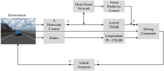
Figure 1: Proposed vision-based automated driving framework. The system comprises the following modules: a multi-task DNN for surrounding perception, vision predictive control and lateral/longitudinal CILQR controllers for vehicle motion planning and adherence to driving commands (steering, acceleration, and braking), and a PI controller combined with the longitudinal CILQR algorithm for velocity tracking. These modules receive input data from a monocular camera and a few cost-effective radars and operate collaboratively to operate the automated vehicle. The DNN, vision predictive control, and lateral and longitudinal CILQR algorithms are run efficiently every 24.52, 15.56, and 0.58 and 0.65 ms, respectively. In our simulation, the end‐to‐end latency from the camera output to the lateral controller output ($T_{a\to b}\equiv T_{lat}$) is longer than the actuator latency ($T_{c\to d}\equiv T_{act}=6.66$ ms).

The constrained iterative linear quadratic regulator (CILQR) method was proposed to solve online trajectory optimization problems with nonlinear system dynamics and general constraints [20, 21]. The CILQR algorithm constructed on the basis of differential dynamic programming (DDP) [22] is also an MPC method. The computational load of the well-established SQP solver is higher than that of DDP [25]. Thus, the CILQR solver outperforms the standard SQP approach in terms of computational efficiency; compared with the CILQR solver, the SQP approach requires a computation time that is 40.4 times longer per iteration [21]. However, previous CILQR-relates studies [20, 21, 23, 24, 25] have focused on nonlinear Cartesian-frame motion planning. Alternatively, planning within the Frenét-frame can reduce problem dimensions because it enables vehicle dynamics to be solved in tangential and normal directions separately with the aid of road reference line [26, 27]; furthermore, the corresponding linear dynamic equations [18, 28] do not have adverse effects when high-order Taylor expansion coefficients are truncated in the CILQR framework [cf. Section II]. These considerations motivated us to use linear CILQR planners to control automated vehicles.

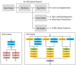
Figure 2: Overview of proposed MTUNet architecture. The input RGB image of size 228 $\times$ 228 is fed into the model, which then performs lane line segmentation, ego vehicle’s pose estimation, and traffic object detection at the same time. The backbone-seg-subnet is an UNet-based network; three variants of UNet (UNet$\_$2$\times$ [30], UNet$\_$1$\times$ [40], and MResUNet [40]) are compared in this work. The ReLU activation functions in pose and det subnets are not shown for simplicity.

We proposed an MTDNN in [29] to directly perceive ego vehicle’s heading angle ($\theta$) and distance from the lane centerline ($\Delta$) for autonomous driving. The vision-based MTDNN model in [29] essentially provides the information necessary for ego car navigation within Frenét coordinates without the need for HD maps. Nevertheless, this end-to-end driving approach performs poorly in environments that are not shown during the training phase [2]. In [30], we proposed an improved control algorithm based on a multi-task UNet architecture (MTUNet) that comprises lane line segmentation and pose estimation subnets. A Stanley controller [32] was then designed to control the lateral automation of an automobile. The Stanley controller takes $\theta$ and $\Delta$ yielding from the network as it’s input for lane-centering [31]. The improved algorithm outperforms the model in [29] and has comparable performance to a multi-task-learning reinforcement-learning (MTL-RL) model [33], which integrates RL and deep-learning algorithms for autonomous driving. However, our algorithms presented in [30] have some known problems: 1) Vehicle dynamic models are not considered in the Stanley controller, and the model has poor performance for lanes with rapid curvature changes [34]. 2) The proposed self-driving system does not consider road curvature, resulting in poor vehicle control on curvy roads [35]. 3) The corresponding DNN perception network lacks object detection capability, which is a core task in automated driving. 4) The DNN input has high dimensional resolution of 400 $\times$ 400, which results in long training and inference times.

To address these shortcomings, we propose a new system for real-time automated driving on the basis of the developments described in [30, 31]. First, a YOLOv4 detector [36] is added to the MTUNet for object detection. Second, we increase the inference speed of MTUNet by reducing the input size without sacrificing network performance. Third, the vision predictive control (VPC) algorithm is proposed for reducing the steering command delay by enabling steer correction at a look-ahead point on the basis of road curvature information. The VPC algorithm can also be combined with the lateral CILQR algorithm (denoted VPC-CILQR) to rapidly perform motion planning and automobile control. As shown in Fig. 1, the vehicle actuation latency ($T_{act}$) is shorter than the steering command latency ($T_{lat}$) in our simulation. This delay can also occur in automated vehicles [37] or autonomous racing systems [38] and may cause instability of the controlled system [39]. Equipping the vehicle with low-level computers could further increase this steering command lag. Therefore, compensating algorithms such as VPC are key to cost-efficient automated vehicle systems.

The main goal of this work was to design an automated driving system that can operate efficiently in real-time lane-keeping and car-following scenarios. The contributions of this paper are as follows:

1. The proposed MTDNN scheme can execute simultaneous driving perception tasks at a speed of 40 FPS. The main difference between this scheme and previous MTDNN schemes is that the post-processing methods provide crucial parameters (lateral offset, road curvature, and heading angle) that improve local vehicular navigation.

2. The VPC-CILQR controller comprising the VPC algorithm and lateral CILQR solver is proposed to improve driverless vehicle path tracking. The method has a low online computational burden and can respond to steering commands in accordance with the concept of look-ahead distance.

3. We propose a vision-based framework comprising the aforementioned MTDNN scheme and CILQR-based controllers for operating an autonomous vehicle; the effectiveness of the proposed framework was demonstrated in challenging simulation environments without maps.

II Methodology

The following section introduces each part of the proposed self-driving system. As depicted in Fig. 1, our system comprises several modules. The DNN is an MTUNet that can solve multiple perception problems simultaneously. The CILQR controllers receive data from the DNN and radars to compute driving commands for lateral and longitudinal motion planning. In the lateral direction, the lane line detection results from the DNN are input to the VPC module to compute steering angle corrections at a certain distance in front of the ego car. These corrections are then sent to the CILQR solver to predict a steering angle for the lane-keeping task. This two-step algorithm is denoted VPC-CILQR throughout the article. The other CILQR controller handles the car-following task in the longitudinal direction.

II-A MTUNet network

As indicated in Fig. 2, the proposed MTDNN is a neural network with an MTUNet architecture featuring a common backbone encoder and three subnets for completing multiple tasks at the same time. The following sections describe each part.

II-A1 Backbone and segmentation subnet

The shared backbone and segmentation (seg) subnet employ encoder-decoder UNet-based networks for pixel-level lane line classification task. Two classical UNets (UNet$\_$2$\times$ [30] and UNet$\_$1$\times$ [40]) and one enhanced version (MultiResUNet [40], denoted as MResUNet throughout the paper) were used to investigate the effects of model size and complexity on task performance. For UNet$\_$2$\times$ and UNet$\_$1$\times$, each repeated block includes two convolutional (Conv) layers, and the first UNet has twice as many filters as the second. For MResUNet, each modified block consists of three 3 $\times$ 3 Conv layers and one 1 $\times$ 1 Conv layer. Table I summarizes the filter number and related kernel size of the Conv layers used in these models. The resulting total number of parameters of UNet$\_$2$\times$/UNet$\_$1$\times$/MResUNet is 31.04/7.77/7.26 M, and the corresponding total number of multiply-and-accumulates (MACs) is 38.91/9.76/12.67 G. All 3 $\times$ 3 Conv layers we used are padded with one pixel to preserve the spatial resolution after convolution operations [41]. This setting reduces the network input size from 400 $\times$ 400 to 228 $\times$ 228 but preserves model performance and achieves faster inference compared with in our previous work (the experimental results are presented in Section IV) [30], where the network utilizes unpadded 3 $\times$ 3 Conv layers [42], and zero padding must be applied to the input to equalize the input-output resolutions [43]. In the training phase, the weighted cross-entropy loss is adopted to deal with the lane detection sample imbalance problem [44, 45] and is represented as

$$\begin{split}L_{S}=&-\frac{N^{-}}{N^{+}+N^{-}}\sum\limits_{\tilde{y}=1}\log\left(\sigma(y)\right)\\ &-\frac{N^{+}}{N^{+}+N^{-}}\sum\limits_{\tilde{y}=0}\log\left(1-\sigma(y)\right),\end{split}$$ (1)

where $N^{+}$ and $N^{-}$ are numbers of foreground and background samples in a batch of images, respectively; $y$ is a predicted score; $\tilde{y}$ is the corresponding label; and $\sigma$ is the sigmoid function.

II-A2 Pose subnet

This subnet is mainly responsible for whole-image angle regression and road type classification problems, where the road involves three categories (left turn, straight, and right turn) designed to prevent the angle estimation from mode collapsing [30, 46]. The network architecture of the pose subnet is presented in Fig. 2; the pose subnet takes the fourth Conv-block output feature maps of the backbone as its input. Subsequently, the input maps are fed into shared parts including two consecutive Conv layers and one global average pooling (GAP) layer to extract general features. Lastly, the resulting vectors are passed separately through two fully connected (FC) layers before being mapped into a sigmoid/softmax activation layer for the regression/classification task. Table II summarizes the number of filters and output units of the corresponding Conv and FC layers, respectively. The expression MTUNet$\_$2$\times$/MTUNet$\_$1$\times$/MTMResUNet in Table II represents a multi-task UNet scheme in which subnets are built on the UNet$\_$2$\times$/UNet$\_$1$\times$/MResUNet model throughout the article. The pose task loss function, including L2 regression loss ($L_{R}$) and cross-entropy loss ($L_{C}$), is employed for network training; this function is represented as follows:

$$L_{R}=\frac{1}{{2B}}\sum\limits_{i=1}^{B}{\left|{\sigma(\tilde{\theta}_{i})-\sigma(\theta_{i})}\right|^{2}},$$ (2a)

$$L_{C}=-\frac{1}{B}\sum\limits_{i=1}^{B}\sum\limits_{j=1}^{3}\tilde{p}_{ij}\log(p_{ij}),$$ (2b)

where $\tilde{\theta}$ and $\theta$ are the ground truth and estimated value, respectively; $B$ is the input batch size; and $\tilde{p}$ and $p$ are true and softmax estimation values, respectively.

II-A3 Detection subnet

The detection (det) subnet takes advantage of a simplified YOLOv4 detector [36] for real-time traffic object (leading car) detection. This fully-convolutional subnet that has three branches for multi-scale detection takes the output feature maps of the backbone as its input, as illustrated in Fig. 2. The initial part of each branch is composed of single or consecutive 3 $\times$ 3 filters for extracting contextual information at different scales [40], and a shortcut connection with one 1 $\times$ 1 filter from the input layer for residual mapping. The top of the addition layer contains sequential 1 $\times$ 1 filters for reducing the number of channels. The resulting feature maps of each branch have six channels (five for bounding box offset and confidence score predictions, and one for class probability estimation) with a size of $K$ = 15 $\times$ 15 to divide the input image into $K$ grids. In this article, we select $M$ = 3 anchor boxes, which are then shared between three branches according to the context size. Ultimately, spatial features from three detecting scales are concatenated together and sent to the output layer. Table III presents the design of detection subnet of MTUNets. The overall loss function for training comprises objectness ($L_{O}$), classification ($L_{CL}$), and complete intersection over union (CIoU) losses ($L_{CI}$) [47, 48, 49]; these losses are constructed as follows:

$$\begin{split}L_{O}=&-\sum\limits_{i=1}^{K\times M}{{I_{i}^{o}\left[{\tilde{Q}_{i}\log\left({Q_{i}}\right)}\right.}}\left.{+\left({1-\tilde{Q}_{i}}\right)\log\left({1-Q_{i}}\right)}\right]\\ &-{{\lambda_{n}I_{i}^{n}\left[{\tilde{Q}_{i}\log\left({Q_{i}}\right)}\right.}}\left.{+\left({1-\tilde{Q}_{i}}\right)\log\left({1-Q_{i}}\right)}\right],\\ \end{split}$$ (3a)

$$\begin{split}L_{CL}=&-\sum\limits_{i=1}^{K\times M}{I_{i}^{o}\sum\limits_{c\in classes}{{\tilde{p}_{i}\left(c\right)\log\left({p_{i}\left(c\right)}\right)}}}\\ &+\left({1-\tilde{p}_{i}\left(c\right)}\right)\log\left({1-p_{i}\left(c\right)}\right),\end{split}$$ (3b)

$$L_{CI}=1-IoU+\frac{{E^{2}\left({{\bf\tilde{o}},{\bf o}}\right)}}{{\beta^{2}}}+\alpha\gamma,$$ (3c)

where $I_{i}^{o/n}$ = 1/0 or 0/1 indicates that the $i$-th predicted bounding box does or does not contain an object, respectively; $\tilde{Q}_{i}$/$Q_{i}$ and $\tilde{p}_{i}$/$p_{i}$ are the true/estimated objectness and class scores corresponding to each box, respectively; and $\lambda_{n}$ is a hyperparameter intended for balancing positive and negative samples. With regard to CIoU loss, ${\bf\tilde{o}}$ and ${\bf o}$ are the central points of the prediction ($B_{p}$) and ground truth ($B_{gt}$) boxes, respectively; $E$ is the related Euclidean distance; $\beta$ is the diagonal distance of the smallest enclosing box covering $B_{p}$ and $B_{gt}$; $\alpha$ is a tradeoff hyperparameter; and $\gamma$ is used to measure aspect ratio consistency [47].

TABLE I: Conv layers used in the UNet-based networks

Conv-block	UNet$\_$2$\times$ [30]	UNet$\_$1$\times$ [40]	MResUNet [40]
Block$1^{a}$/9	64 (3 $\times$ 3)b	32 (3 $\times$ 3)	8 (3 $\times$ 3), 17 (3 $\times$ 3),
	64 (3 $\times$ 3)	32 (3 $\times$ 3)	26 (3 $\times$ 3), 51 (1 $\times$ 1)
Block2/8	128 (3 $\times$ 3)	64 (3 $\times$ 3)	17 (3 $\times$ 3), 35 (3 $\times$ 3),
	128 (3 $\times$ 3)	64 (3 $\times$ 3)	53 (3 $\times$ 3), 105 (1 $\times$ 1)
Block3/7	256 (3 $\times$ 3)	128 (3 $\times$ 3)	35 (3 $\times$ 3), 71 (3 $\times$ 3),
	256 (3 $\times$ 3)	128 (3 $\times$ 3)	106 (3 $\times$ 3), 212 (1 $\times$ 1)
Block4/6	512 (3 $\times$ 3)	256 (3 $\times$ 3)	71 (3 $\times$ 3), 142 (3 $\times$ 3),
	512 (3 $\times$ 3)	256 (3 $\times$ 3)	213 (3 $\times$ 3), 426 (1 $\times$ 1)
Block5	1024 (3 $\times$ 3)	512 (3 $\times$ 3)	142 (3 $\times$ 3), 284 (3 $\times$ 3),
	1024 (3 $\times$ 3)	512 (3 $\times$ 3)	427 (3 $\times$ 3), 853 (1 $\times$ 1)
aBlock1 of UNet$\_$2$\times$/UNet$\_$1$\times$ only contains one 3 $\times$ 3 Conv layer
bThe notation $n$ ($k$ $\times$ $k$) represents a Conv layer with $n$ filters of kernal size $k$ $\times$ $k$

TABLE II: Conv and FC layers used in the pose subnet of various MTUNets

Layer	MTUNet$\_$2$\times$	MTUNet$\_$1$\times$
		MTMResUNet
Conv1	1024 (3 $\times$ 3)	512 (3 $\times$ 3)
Conv2	1024 (3 $\times$ 3)	512 (3 $\times$ 3)
FC1-2	256, 256	256, 256
FC3-4	1, 3	1, 3

TABLE III: Conv layers used in the detection subnet of various MTUNets

Layer	MTUNet$\_$2$\times$	MTUNet$\_$1$\times$
		MTMResUNet
Conv1-6	512 (3 $\times$ 3)	384 (3 $\times$ 3)
Conv7-9	512 (1 $\times$ 1)	384 (1 $\times$ 1)
Conv10-12	256 (1 $\times$ 1)	256 (1 $\times$ 1)
Conv13-15	256 (1 $\times$ 1)	256 (1 $\times$ 1)
Conv16-18	6 (1 $\times$ 1)	6 (1 $\times$ 1)

II-B The CILQR algorithm

This section first briefly describes the concept behind CILQR and related approaches based on Ref. [20, 21, 50, 51]; it then presents the lateral/longitudinal CILQR control algorithm that takes the MTUNet inference and radar data as its inputs to yield driving decisions using linear dynamics.

II-B1 Problem formulation

Provided a sequence of states ${\bf X}\equiv\left\{{{\bf x}_{0},{\bf x}_{1},...,{\bf x}_{N}}\right\}$ and the corresponding control sequence ${\bf U}\equiv\left\{{{\bf u}_{0},{\bf u}_{1},...,{\bf u}_{N-1}}\right\}$ are within the preview horizon $N$, the system’s discrete-time dynamics ${\bf f}$ are satisfied, with

$${\bf x}_{i+1}={\bf f}\left({{\bf x}_{i},{\bf u}_{i}}\right)$$ (4)

from time $i$ to $i+1$. The total cost denoted by $\mathcal{J}$, including running costs $\mathcal{P}$ and the final cost $\mathcal{P}_{f}$, is presented as follows:

$$\mathcal{J}\left({{\bf x}_{0},{\bf U}}\right)=\sum\limits_{i=0}^{N-1}{\mathcal{P}\left({{\bf x}_{i},{\bf u}_{i}}\right)+\mathcal{P}_{f}\left({{\bf x}_{N}}\right)}.$$ (5)

The optimal control sequence is then written as

$${\bf U}^{*}\left({{\bf x}^{*}}\right)\equiv\mathop{\arg\min}\limits_{\bf U}\mathcal{J}\left({{\bf x}_{0},{\bf U}}\right)$$ (6)

with an optimal trajectory ${{\bf x}^{*}}$. The partial sum of $\mathcal{J}$ from any time step $t$ to $N$ is represented as

$$\mathcal{J}_{t}\left({{\bf x},{\bf U}_{t}}\right)=\sum\limits_{i=t}^{N-1}{\mathcal{P}\left({{\bf x}_{i},{\bf u}_{i}}\right)+\mathcal{P}_{f}\left({{\bf x}_{N}}\right)},$$ (7)

and the optimal value function $\mathcal{V}$ at time $t$ starting at ${\bf x}$ takes the form

$$\mathcal{V}_{t}\left({\bf x}\right)\equiv\mathop{\arg\min}\limits_{{\bf U}_{t}}\mathcal{J}_{t}\left({{\bf x},{\bf U}_{t}}\right)$$ (8)

with the final time step value function $\mathcal{V}_{N}\left({\bf x}\right)\equiv\mathcal{P}_{f}\left({{\bf x}_{N}}\right)$.

In practice, the final step value function $\mathcal{V}_{N}\left({\bf x}\right)$ is obtained by executing a forward pass using the current control sequence. Subsequently, local control signal minimizations are performed in the proceeding backward pass using the following Bellman equation:

$$\mathcal{V}_{i}\left({\bf x}\right)=\mathop{\min}\limits_{\bf u}\left[{\mathcal{P}\left({{\bf x},{\bf u}}\right)+\mathcal{V}_{i+1}\left({{\bf f}\left({{\bf x},{\bf u}}\right)}\right)}\right].$$ (9)

To compute the optimal trajectory, the perturbed function around the $i$-th state-control pair in Eq. (9) is used; this function is written as follows:

$$\begin{split}\mathcal{O}\left({\delta{\bf x},\delta{\bf u}}\right)=&\mathcal{P}_{i}\left({{\bf x}+\delta{\bf x},{\bf u}+\delta{\bf u}}\right)-\mathcal{P}_{i}\left({{\bf x},{\bf u}}\right)\\ &+\mathcal{V}_{i+1}\left({{\bf f}\left({{\bf x}+\delta{\bf x},{\bf u}+\delta{\bf u}}\right)}\right)-\mathcal{V}_{i+1}\left({{\bf f}\left({{\bf x},{\bf u}}\right)}\right).\end{split}$$ (10)

This equation can be approximated to a quadratic function by employing a second-order Taylor expansion with the following coefficients:

$$\mathcal{O}_{\bf x}=\mathcal{P}_{\bf x}+{\bf f}_{\bf x}^{\rm T}\mathcal{V}_{\bf x},$$ (11a)

$$\mathcal{O}_{\bf u}=\mathcal{P}_{\bf u}+{\bf f}_{\bf u}^{\rm T}\mathcal{V}_{\bf x},$$ (11b)

$$\mathcal{O}_{{\bf xx}}=\mathcal{P}_{{\bf xx}}+{\bf f}_{\bf x}^{\rm T}\mathcal{V}_{{\bf xx}}{\bf f}_{\bf x}+\mathcal{V}_{\bf x}{\bf f}_{{\bf xx}},$$ (11c)

$$\mathcal{O}_{{\bf ux}}=\mathcal{P}_{{\bf ux}}+{\bf f}_{\bf u}^{\rm T}\mathcal{V}_{{\bf xx}}{\bf f}_{\bf x}+\mathcal{V}_{\bf x}{\bf f}_{{\bf ux}},$$ (11d)

$$\mathcal{O}_{{\bf uu}}=\mathcal{P}_{{\bf uu}}+{\bf f}_{\bf u}^{\rm T}\mathcal{V}_{{\bf xx}}{\bf f}_{\bf u}+\mathcal{V}_{\bf x}{\bf f}_{{\bf uu}}.$$ (11e)

The second-order coefficients of the system dynamics (${\bf f}_{\bf xx}$, ${\bf f}_{\bf ux}$, and ${\bf f}_{\bf uu}$) are omitted to reduce computational effort [25, 50]. The values of these coefficients are zero for linear systems [e.g., Eq. (19) and Eq. (25)], leading to fast convergence in trajectory optimization.

The optimal control signal modification can be obtained by minimizing the quadratic $\mathcal{O}\left({\delta{\bf x},\delta{\bf u}}\right)$:

$$\delta{\bf u}^{*}=\mathop{\arg\min}\limits_{\delta{\bf u}}\mathcal{O}\left({\delta{\bf x},\delta{\bf u}}\right)={\bf k}+{\bf K}\delta{\bf x},$$ (12)

where

$${\bf k}=-\mathcal{O}_{{\bf uu}}^{-1}\mathcal{O}_{\bf u},$$ (13a)

$${\bf K}=-\mathcal{O}_{{\bf uu}}^{-1}\mathcal{O}_{{\bf ux}}$$ (13b)

are optimal control gains. If the optimal control indicated in Eq. (12) is plugged into the approximated $\mathcal{O}\left({\delta{\bf x},\delta{\bf u}}\right)$ to recover the quadratic value function, the corresponding coefficients can be obtained [52]:

$$\mathcal{V}_{\bf x}=\mathcal{O}_{\bf x}-{\bf K}^{\rm T}\mathcal{O}_{{\bf uu}}{\bf k},$$ (14a)

$$\mathcal{V}_{{\bf xx}}=\mathcal{O}_{{\bf xx}}-{\bf K}^{\rm T}\mathcal{O}_{{\bf uu}}{\bf K}.$$ (14b)

Control gains at each state (${\bf k}_{i}$, ${\bf K}_{i}$) can then be estimated by recursively computing Eq. (11), (13), and (14) in a backward process. Finally, the modified control and state sequences can be evaluated through a renewed forward pass:

$${\bf\hat{u}}_{i}={\bf u}_{i}+\lambda{\bf k}_{i}+{\bf K}_{i}\left({{\bf\hat{x}}_{i}-{\bf x}_{i}}\right),$$ (15a)

$${\bf\hat{x}}_{i+1}={\bf f}\left({{\bf\hat{x}}_{i},{\bf\hat{u}}_{i}}\right),$$ (15b)

where ${\bf\hat{x}}_{0}={\bf x}_{0}$. Here $\lambda$ is the backtracking parameter for line search; it is set to 1 in the beginning and designed to be reduced gradually in the forward-backward propagation loops until convergence is reached.

If the system has the constraint

$$\mathcal{C}\left({x,u}\right)<0,$$ (16)

which can be shaped using an exponential barrier function [20, 23]

$$\mathcal{B}\left({\mathcal{C}\left({x,u}\right)}\right)=q_{1}\exp\left({q_{2}\mathcal{C}\left({x,u}\right)}\right)$$ (17)

or a logarithmic barrier function [21], then

$$\mathcal{B}\left({\mathcal{C}\left({x,u}\right)}\right)=-\frac{1}{t}\log\left({-\mathcal{C}\left({x,u}\right)}\right),$$ (18)

where $q_{1}$, $q_{2}$, and $t>0$ are parameters. The barrier function can be added to the cost function as a penalty. Eq. (18) converges toward the ideal indicator function as $t$ increases iteratively.

II-B2 Lateral CILQR controller

The lateral vehicle dynamic model [28] is employed for steering control. The state variable and control input are defined as ${\bf x}=\left[{\begin{array}[]{*{20}c}\Delta&{\dot{\Delta}}&\theta&{\dot{\theta}}\\ \end{array}}\right]^{\rm T}$ and ${\bf u}=\left[\delta\right]$, respectively, where $\Delta$ is the lateral offset, $\theta$ is the angle between the ego vehicle’s heading and the tangent of the road, and $\delta$ is the steering angle. As described in our previous work [30, 31], $\theta$ and $\Delta$ can be obtained from MTUNets and related post-processing methods, and it is assumed that $\dot{\Delta}=\dot{\theta}=0$. The corresponding discrete-time dynamic model is written as follows:

$${\bf x}_{t+1}\equiv{\bf f}\left({{\bf x}_{t},{\bf u}_{t}}\right)={\bf Ax}_{t}+{\bf Bu}_{t},$$ (19)

where

$${\bf A}=\left[{\begin{array}[]{*{20}c}{\alpha_{11}}&{\alpha_{12}}&0&0\\ 0&{\alpha_{22}}&{\alpha_{23}}&{\alpha_{24}}\\ 0&0&{\alpha_{33}}&{\alpha_{34}}\\ 0&{\alpha_{42}}&{\alpha_{43}}&{\alpha_{44}}\\ \end{array}}\right],\quad{\bf B}=\left[{\begin{array}[]{*{20}c}0\\ {\beta_{1}}\\ 0\\ {\beta_{2}}\\ \end{array}}\right],$$

with coefficients

$$\begin{array}[]{l}\alpha_{11}=\alpha_{33}=1,\quad\alpha_{12}=\alpha_{34}=dt,\\ \alpha_{22}={1-\frac{{2\left({C_{\alpha f}+C_{\alpha r}}\right)dt}}{{mv}}},\quad\alpha_{23}={\frac{{2\left({C_{\alpha f}+C_{\alpha r}}\right)dt}}{m}},\\ \alpha_{24}={\frac{{2\left({-C_{\alpha f}l_{f}+C_{\alpha r}l_{r}}\right)dt}}{{mv}}},\quad\alpha_{42}={\frac{{2\left({C_{\alpha f}l_{f}-C_{\alpha r}l_{r}}\right)dt}}{{I_{z}v}}},\\ \alpha_{43}={\frac{{2\left({C_{\alpha f}l_{f}-C_{\alpha r}l_{r}}\right)dt}}{{I_{z}}}},\quad\alpha_{44}={1-\frac{{2\left({C_{\alpha f}l_{f}^{2}-C_{\alpha r}l_{r}^{2}}\right)dt}}{{I_{z}v}}},\\ \beta_{1}={\frac{{2C_{\alpha f}dt}}{m}},\quad\beta_{2}={\frac{{2C_{\alpha f}l_{f}dt}}{{I_{z}}}}.\\ \end{array}$$

Here, $v$ is the ego vehicle’s current speed along the heading direction and $dt$ is the sampling time. The model parameters for the experiments are as follows: vehicle mass $m$ = 1150 kg, cornering stiffness ${C_{\alpha f}}$ = 80 000 N/rad, ${C_{\alpha r}}$ = 80 000 N/rad, center of gravity point $l_{f}$ = 1.27 m, $l_{r}$ = 1.37 m, and moment of inertia $I_{z}$ = 2000 kgm².

The objective function ($\mathcal{J}$) containing the iterative linear quadratic regulator ($\mathcal{J}_{ILQR}$), barrier ($\mathcal{J}_{b}$), and end state cost ($\mathcal{J}_{f}$) terms can be represented as

$$\mathcal{J}=\mathcal{J}_{ILQR}+\mathcal{J}_{b}+\mathcal{J}_{f},$$ (20a)

$$\mathcal{J}_{ILQR}=\sum\limits_{i=0}^{N-1}{\left({{\bf x}_{i}-{\bf x}_{r}}\right)^{\rm T}{\bf Q}\left({{\bf x}_{i}-{\bf x}_{r}}\right)+{\bf u}_{i}^{\rm T}{\bf Ru}_{i}},$$ (20b)

$$\mathcal{J}_{b}=\sum\limits_{i=0}^{N-1}{\mathcal{B}\left(u_{i}\right)+\mathcal{B}\left(\Delta_{i}\right)},$$ (20c)

$$\mathcal{J}_{f}=\left({{\bf x}_{N}-{\bf x}_{r}}\right)^{\rm T}{\bf Q}\left({{\bf x}_{N}-{\bf x}_{r}}\right)+\mathcal{B}\left({\Delta_{N}}\right).$$ (20d)

Here, the reference state ${\bf x}_{r}$ = $\mathbf{0}$, ${\bf Q}$/${\bf R}$ is the weighting matrix, and $\mathcal{B}\left(u_{i}\right)$ and $\mathcal{B}\left(\Delta_{i}\right)$ are the corresponding barrier functions:

$$\mathcal{B}\left(u_{i}\right)=-\frac{1}{t}\left({\log\left({u_{i}-\delta_{\min}}\right)+\log\left({\delta_{\max}-u_{i}}\right)}\right),$$ (21a)

$$\mathcal{B}\left({\Delta_{i}}\right)=\left\{\begin{array}[]{l}\exp\left({\Delta_{i}-\Delta_{i-1}}\right)\quad\text{for}\quad\Delta_{0}\geq 0,\\ \exp\left({\Delta_{i-1}-\Delta_{i}}\right)\quad\text{for}\quad\Delta_{0}<0,\\ \end{array}\right.$$ (21b)

where $\mathcal{B}$($u_{i}$) is used to limit control inputs and the high (low) steer bound is $\delta_{\max}\left({\delta_{\min}}\right)={\pi\mathord{\left/{\vphantom{\pi 6}}\right.\kern-1.2pt}6}\left({-{\pi\mathord{\left/{\vphantom{\pi 6}}\right.\kern-1.2pt}6}}\right)$ rad. The objective of $\mathcal{B}\left(\Delta_{i}\right)$ is to control the ego vehicle moving toward the lane center.

The first element of the optimal steering sequence is then selected to define the normalized steering command at a given time as follows:

$${\rm SteerCmd}=\frac{{\delta_{0}^{*}}}{{{\pi\mathord{\left/{\vphantom{\pi 6}}\right.\kern-1.2pt}6}}}.$$ (22)

II-B3 Longitudinal CILQR controller

In the longitudinal direction, a proportional-integral (PI) controller [53]

$$PI(v)=k_{P}e+k_{I}\sum\limits_{i}{e_{i}}$$ (23)

is first applied to the ego car for tracking reference speed $v_{r}$ under cruise conditions, where $e=v-v_{r}$ and $k_{P}$/$k_{I}$ are the tracking error and the proportional/integral gain, respectively. The normalized acceleration command is then given as follows:

$${\rm AcclCmd}=\tanh(PI(v)).$$ (24)

When a slower preceding vehicle is encountered, the AccelCmd must be updated to maintain a safe distance from that vehicle to avoid a collision; for this purpose, we use the following longitudinal CILQR algorithm.

The state variable and control input for longitudinal inter-vehicle dynamics are defined as ${\bf x^{\prime}}=\left[{\begin{array}[]{*{20}c}D&v&a\\ \end{array}}\right]^{\rm T}$ and ${\bf u^{\prime}}=\left[j\right]$, respectively, where $a$, $j=\dot{a}$, and $D$ are the ego vehicle’s acceleration, jerk, and distance to the preceding car, respectively. The corresponding discrete-time system model is written as

$${\bf x^{\prime}}_{t+1}\equiv{\bf f^{\prime}}\left({{\bf x^{\prime}}_{t},{\bf u^{\prime}}_{t}}\right)={\bf A^{\prime}x^{\prime}}_{t}+{\bf B^{\prime}u^{\prime}}_{t}+{\bf C^{\prime}w^{\prime}},$$ (25)

where

$$\begin{array}[]{l}{\bf A^{\prime}}=\left[{\begin{array}[]{*{20}c}1&{-dt}&{-\frac{1}{2}dt^{2}}\\ 0&1&{dt}\\ 0&0&1\\ \end{array}}\right],\quad{\bf B^{\prime}}=\left[{\begin{array}[]{*{20}c}0\\ 0\\ {dt}\\ \end{array}}\right],\\ {\bf C^{\prime}}=\left[{\begin{array}[]{*{20}c}0&{dt}&{\frac{1}{2}dt^{2}}\\ 0&0&0\\ 0&0&0\\ \end{array}}\right],\quad{\bf w^{\prime}}=\left[{\begin{array}[]{*{20}c}0\\ {v_{l}}\\ {a_{l}}\\ \end{array}}\right].\\ \end{array}$$

Here, $v_{l}$/$a_{l}$ is the preceding car’s speed/acceleration, and ${\bf w^{\prime}}$ is the measurable disturbance input [54]. The values of $D$ and $v_{l}$ are measured by the radar; $v$ is known; and $a=a_{l}=0$ is assumed. Here, MTUNets are used to recognize traffic objects, and the radar is responsible for providing precise distance measurements.

The objective function ($\mathcal{J}^{\prime}$) for the longitudinal CILQR controller can be written as,

$$\mathcal{J}^{\prime}=\mathcal{J}^{\prime}_{ILQR}+\mathcal{J}^{\prime}_{b}+\mathcal{J}^{\prime}_{f},$$ (26a)

$$\mathcal{J}^{\prime}_{ILQR}=\sum\limits_{i=0}^{N-1}{\left({{\bf x^{\prime}}_{i}-{\bf x^{\prime}}_{r}}\right)^{\rm T}{\bf Q^{\prime}}\left({{\bf x^{\prime}}_{i}-{\bf x^{\prime}}_{r}}\right)+{\bf u^{\prime}}_{i}^{\rm T}{\bf R^{\prime}u^{\prime}}_{i}},$$ (26b)

$$\mathcal{J}^{\prime}_{b}=\sum\limits_{i=0}^{N-1}{\mathcal{B}^{\prime}\left({u^{\prime}_{i}}\right)+\mathcal{B}^{\prime}\left(D_{i}\right)+\mathcal{B}^{\prime}\left({a_{i}}\right)},$$ (26c)

$$\mathcal{J}_{f}^{\prime}=\left({{\bf x^{\prime}}_{N}-{\bf x^{\prime}}_{r}}\right)^{\rm T}{\bf Q^{\prime}}\left({{\bf x^{\prime}}_{N}-{\bf x^{\prime}}_{r}}\right)+\mathcal{B^{\prime}}\left({D_{N}}\right)+\mathcal{B^{\prime}}\left({a_{N}}\right).$$ (26d)

Here, the reference state ${\bf x^{\prime}}_{r}=\left[{\begin{array}[]{*{20}c}{D_{r}}&{v_{l}}&{a_{l}}\\ \end{array}}\right]$, and $D_{r}$ is the reference distance for safety. ${{\bf Q^{\prime}}}$/${\bf R^{\prime}}$ is the weighting matrix, and $\mathcal{B}^{\prime}\left({u^{\prime}_{i}}\right)$, $\mathcal{B}^{\prime}\left(D_{i}\right),$ and $\mathcal{B}^{\prime}\left({a_{i}}\right)$ are related barrier functions:

$$\mathcal{B}^{\prime}\left({u^{\prime}_{i}}\right)=-\frac{1}{t^{\prime}}\left({\log\left({u^{\prime}_{i}-j_{\min}}\right)+\log\left({j_{\max}-u^{\prime}_{i}}\right)}\right),$$ (27a)

$$\mathcal{B}^{\prime}\left(D_{i}\right)=\exp\left({D_{r}-D_{i}}\right),$$ (27b)

$$\mathcal{B}^{\prime}\left({a_{i}}\right)=\exp\left({a_{\min}-a_{i}}\right)+\exp\left({a_{i}-a_{\max}}\right),$$ (27c)

where $\mathcal{B}^{\prime}\left(D_{i}\right)$ is used for maintaining a safe distance, and $\mathcal{B}^{\prime}$($u^{\prime}_{i}$) and $\mathcal{B}^{\prime}$($a_{i}$) are used to limit the ego vehicle’s jerk and acceleration to [$-$1, 1] m/s³ and [$-$5, 5] m/s², respectively.

The first element of the optimal jerk sequence is then chosen to update AccelCmd in the car-following scenario as

$${\rm AcclCmd}=\tanh\left({PI\left(v\right)}\right)+j_{0}^{*}.$$ (28)

The brake command (BrakeCmd) gradually increases in value from 0 to 1 when $D$ is smaller than a certain critical value $D=D_{c}<D_{r}$ in times of emergency.

II-C The VPC algorithm

The problematic scenario for the VPC algorithm is depicted in Fig. 3, which presents a top-down view of fitted lane lines produced using our previous method [31]. First, the detected line segments [Fig. 3(a)] are clustered using the density-based spatial clustering of applications with noise (DBSCAN) algorithm [55]. Second, the resulting semantic lanes are transformed into BEV space by using a perspective transformation. Third, the least-squares quadratic polynomial fitting method is employed to produce parallel ego-lane lines [Fig. 3(b)]; either of the two polynomials can be represented as $y=f(x)$. Fourth, the road curvature $\kappa$ at $x=x_{c}$ is computed using the formula

$$\kappa=\frac{{f^{\prime\prime}}}{{\left({1+f^{\prime 2}}\right)^{{3\mathord{\left/{\vphantom{32}}\right.\kern-1.2pt}2}}}}.$$ (29)

Because the curvature estimate from a single map is noisy, an average map from eight consecutive frames is used for curve fitting. The resulting curvature estimates are then used to determine the correction value of the steering command in this study.

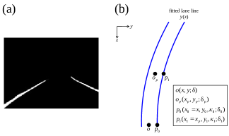
Figure 3: Problematic scenario for the VPC algorithm. (a) An example DNN output lane line binary map at a given time in the egocentric view. (b) Aerial view of fitted lane lines. Here, $o$ and $o_{p}$ are the current position of the ego vehicle and the look-ahead point, respectively, and positions $p_{0}$ and $p_{1}$ represent lane points at the same $x$ coordinates as $o$ and $o_{p}$, respectively. $\kappa$ and $\rm\delta$ are the curvature and steering angle of the vehicle and lane points, respectively. In this paper, the look-ahead distance $\overline{oo_{p}}$ = 10 m is used, which corresponds to a car speed of approximately 72 km/h [28].

As shown in Fig. 3(b), $\delta$ at $o$ is the current steering angle. The desired steering angles at $p_{0}$ and $p_{1}$ can be computed using the local lane curvature [21]:

$$\delta_{0}=\tan^{-1}\left({c\kappa_{0}}\right),$$ (30a)

$$\delta_{1}=\tan^{-1}\left({c\kappa_{1}}\right),$$ (30b)

where $c$ is an adjustable parameter. Hence, the predicted steering angle at a look-ahead point $o_{p}$ can be represented as

$${\delta_{p}}=\delta+\left({\delta_{1}-\delta_{0}}\right)\equiv\delta+\Delta\delta.$$ (31)

Compared to existing LQR-based preview control methods [56, 57], the VPC algorithm has fewer tuning parameters, and can be combined with other path tracking models. For example, VPC-CILQR controller can update the CILQR steering command [Eq. (22)] as follows:

$$\begin{array}[]{l}{\rm VPC\_SteerCmd}\\ =\left\{\begin{array}[]{l}{\rm SteerCmd}+\left|{\Delta\delta}\right|{\rm\quad if\quad SteerCmd}\geq{\rm 0,}\\ {\rm SteerCmd}-\left|{\Delta\delta}\right|{\rm\quad if\quad SteerCmd}<{\rm 0}{\rm.}\\ \end{array}\right.\\ \end{array}$$ (32)

TABLE IV: Summary of data sets used in our experiments

Dataset	Scenarios	No. of images	Labels	No. of traffic objects	Sources
CULane	urban,	28368		80437	[61],
	highway		ego-lane lines,		this work
LLAMAS	highway	22714	bounding boxes	29442	[62],
					this work
TORCS		42747	ego-lane lines,	30189	[30]
			bounding boxes,
			ego’s heading,
			road type

III Experimental setup

The proposed MTUNets extract local and global contexts from input images to simultaneously solve segmentation, detection, and pose tasks. Because the learning rates of these tasks are different [43, 58, 59], the proposed MTUNets are trained in a stepwise manner rather than in an end-to-end manner to help the backbone network gradually learn common features. Setups of the training strategy, image data, and dynamic validation are given as follows:

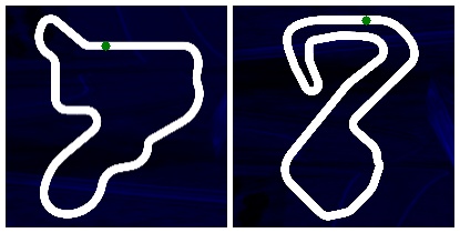
Figure 4: Tracks A (left) and B (right) for dynamically evaluating proposed MTUNet and control models. The total length of Track A/B (Track 7/8 in [30]) was 2843/3919 m with lane width 4 m, and the maximum curvature was approximately 0.03/0.05 1/m, which was curvier than a typical road [66]. The self-driving car drove in a counterclockwise direction, and the starting locations are marked by green filled circle symbols. A self-driving vehicle [33] could not finish a lap on Track A using the direct perception approach [67].

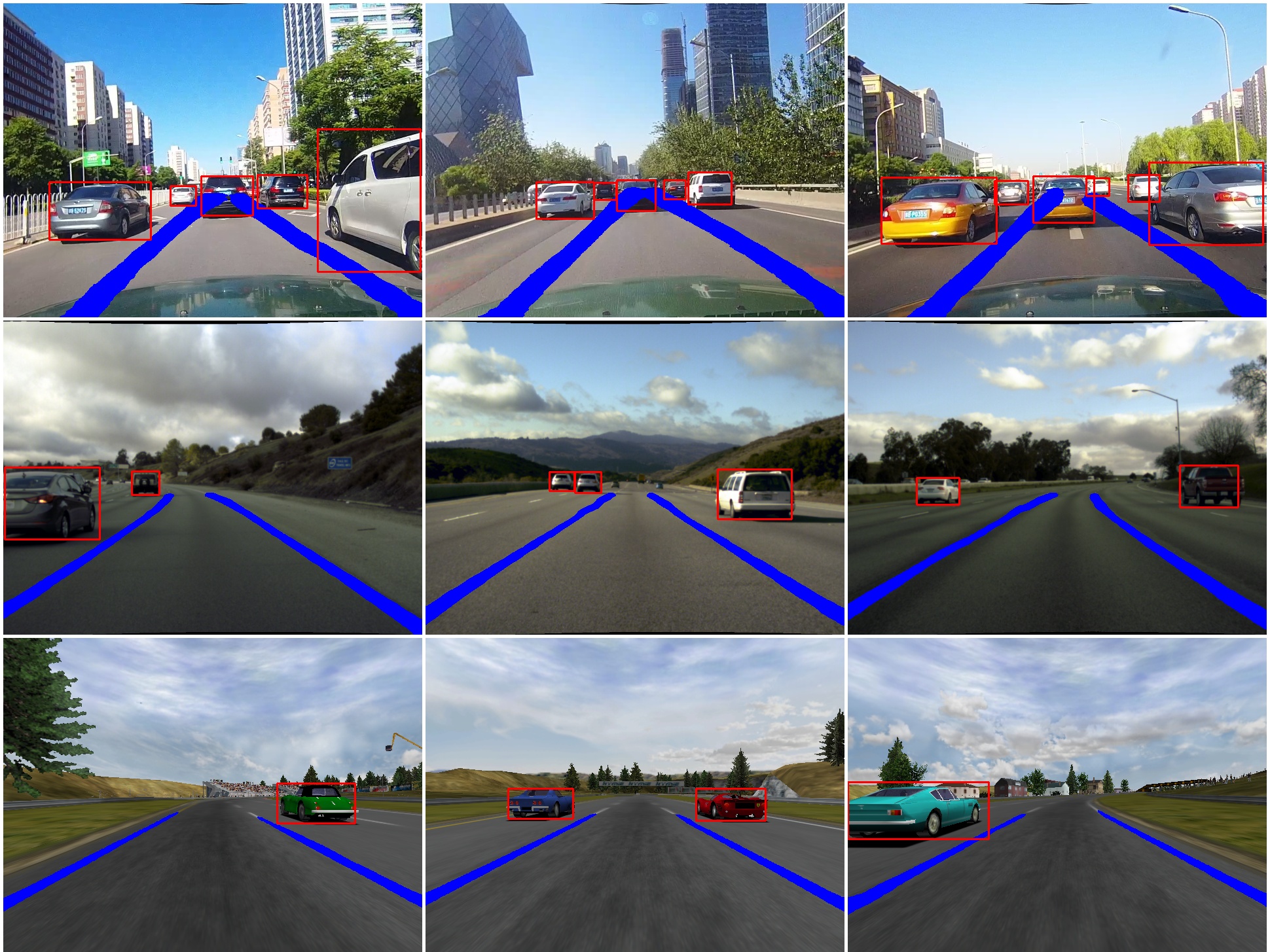
Figure 5: Example traffic object and lane line detection results of the MTUNet$\_$1$\times$ network on CULane (first row), LLAMAS (second row), and TORCS (third row) images.

III-A Network training strategy

The MTUNets are trained through three stages. The pose subnet is first trained through stochastic gradient descent (SGD) with a batch size (bs) of 20, momentum (mo) of 0.9, and learning rate (lr) starting from $10^{-2}$ and decreasing by a factor of 0.9 every 5 epochs for a total of 100 epochs. Detection and pose subnets are then trained jointly based on the trained parameters from the first stage using the SGD optimizer with bs = 4, mo = 0.9, and lr = $10^{-3}$, $10^{-4}$, and $10^{-5}$ for the first 60 epochs, the 61st to 80th epochs, and the last 20 epochs, respectively. All subnets (detection, pose, and segmentation) were trained together in the last stage using the pretrained model from the previous stage using the Adam optimizer. Bs and mo were set to 1 and 0.9, respectively. Lr was set to $10^{-4}$ for the first 75 epochs and $10^{-5}$ for the last 25 epochs. The total loss in each stage is a weighted sum of the corresponding losses [60].

TABLE V: Performance of trained MTUNets on test data

Network	Dataset	Task config.	Det		Seg		Pose
			Recall	AP (%)	Recall	F1 score	Heading	Road type
							MAE (rad)	accuracy (%)
MTUNet$\_$2$\times$	CULane	Det + Seg	0.858	65.32	0.694	0.688	-	-
MTUNet$\_$1$\times$			0.831	58.67	0.658	0.595	-	-
MTMResUNet			0.852	54.28	0.559	0.568	-	-
MTUNet$\_$2$\times$	LLAMAS	Det + Seg	0.942	64.42	0.935	0.827	-	-
MTUNet$\_$1$\times$			0.946	59.96	0.936	0.831	-	-
MTMResUNet			0.950	57.40	0.736	0.748	-	-
MTUNet$\_$2$\times$	TORCS	Pose	-	-	-	-	0.004	90.42
MTUNet$\_$1$\times$			-	-	-	-	0.005	90.48
MTMResUNet			-	-	-	-	0.006	83.77
MTUNet$\_$2$\times$		Det + Seg	0.976	71.51	0.905	0.889	-	-
MTUNet$\_$1$\times$			0.974	66.14	0.904	0.894	-	-
MTMResUNet			0.968	66.12	0.833	0.869	-	-
MTUNet$\_$2$\times$		Det + Seg + Pose	0.952	65.83	0.922	0.883	0.005	87.08
MTUNet$\_$1$\times$			0.956	59.25	0.901	0.882	0.004	94.30
MTMResUNet			0.959	51.88	0.830	0.855	0.007	80.46

III-B Image data sets

We conducted experiments on artificial TORCS [30] and real-world CULane/LLAMAS [61, 62] data sets; the corresponding statistics are summarized in Table IV. The customized TORCS data set has joint labels for all tasks, whereas the original CULane/LLAMAS data set only contained lane line labels. Thus, we annotated each CULane/LLAMAS image with traffic object bounding boxes to imitate the TORCS data. The resulting numbers of labeled traffic objects in the TORCS/CULane/LLAMAS data set were approximately 30K/80K/29K. To determine anchor boxes for the detection task, the $k$-means algorithm [63] was applied to partition ground truth boxes. Nevertheless, the CULane and LLAMAS data sets still lacked the ego vehicle’s angle labels; therefore, these data sets could only be used for comparing segmentation and detection tasks. The ratio of the number of images used in the training phase to that used in the test phase was approximately 10 for both data sets, as in our previous works [30, 31]. Recall/average precision (AP; IoU was set to 0.5) [64], recall/F1 score [45], and accuracy/mean absolute error (MAE) [30] were used to evaluate model performance in detection, segmentation, and pose tasks, respectively.

III-C Autonomous driving simulation

The open-source driving environment TORCS provides sophisticated physics and graphics engines, making it ideal for not only visual processing but also vehicle dynamics research [65]. Thus, the ego vehicle controlled by our self-driving framework comprising trained MTUNets and proposed controllers could drive autonomously on unseen TORCS roads [e.g., Track A and B in Fig. 4] to verify the effectiveness of our approach. All experiments, including MTUNets training, testing, and driving simulation were conducted on a PC equipped with an INTEL i9-9900K CPU, 64 GB of RAM, and an NVIDIA RTX 2080 Ti GPU. The control frequency for the ego vehicle in TORCS was approximately 150 Hz on our computer.

TABLE VI: Results for MTUNets in terms of parameters (Params), multiply-and-accumulates (MACs), and frames per second (FPS)

Network	Task config.	Params	MACs	FPS
MTUNet$\_$$2\times$	Pose	19.37 M	13.93 G	74.02
MTUNet$\_$$1\times$		4.98 M	3.51 G	122.72
MTMResUNet		5.37 M	2.70 G	99.08
MTUNet$\_$$2\times$	Det + Seg	68.62 M	47.36 G	24.44
MTUNet$\_$$1\times$		21.70 M	12.89 G	43.58
MTMResUNet		21.97 M	15.98 G	27.79
MTUNet$\_$$2\times$	Det + Seg + Pose	83.31 M	50.55 G	23.28
MTUNet$\_$$1\times$		25.50 M	13.69 G	40.77
MTMResUNet		26.56 M	16.95 G	27.30

TABLE VII: Dynamic system models and parameters for CILQR and SQP controllers implementation

	Lateral	Longitudinal
	CILQR-/SQP-based	CILQR/SQP
Dynamic model	Eq. (19)	Eq. (25)
Sampling time ($dt$)	0.05 s	0.1 s
Pred. horizon ($N$)	30	30
Ref. dist. ($D_{r}$)	-	11 m
Weighting matrixes	${\bf Q}$ = ${\rm diag}\left({20,1,20,1}\right)$	${{\bf Q^{\prime}}}$ = ${\rm diag}\left({20,20,1}\right)$
	${\bf R}=\left[1\right]$	${\bf R^{\prime}}=\left[1\right]$

IV Results and discussions

Table V presents the performance results of MTUNet models when applied to the testing data for various task configurations. Table VI presents the number of parameters, computational complexity, and inference speed of all schemes for computational efficiency comparison. As described in Section II, although we reduced the input size of the MTUNet models by using padded 3 $\times$ 3 Conv layers, which does not affect model performance, MTUNet$\_$2$\times$/MTUNet$\_$1$\times$ had similar results to our previous model for the segmentation and pose tasks on the TORCS and LLAMAS datasets [30]. For complex CULane data, the MTUNet model performance was worse than that of the SCNN [61], the original state-of-the-art method applied to this dataset; however, the SCNN has lower inference speed due to its higher computational complexity [10]. The MTUNet models are designed for real-time control of self-driving vehicles; the SCNN model is not. Of the three considered MTUNet variants, MTUNet$\_$2$\times$ and MTUNet$\_$1$\times$ outperformed MTMResUNet on all data sets when each model jointly performed detection and segmentation tasks (first, second, and fourth row of Table V); this finding differs from the single-segmentation-task analysis results for biomedical images [40]. Because task gradient interference often reduces the performance of an MTDNN [68, 69], the MTUNet$\_$2$\times$ and MTUNet$\_$1$\times$ models outperformed the complicated MTMResUNet network because of their elegant architecture. When the pose task was included (last row of Table V), MTUNet$\_$2$\times$ and MTUNet$\_$1$\times$ also outperformed MTMResUNet for all evaluation metrics; the decreasing AP scores for the detection task are attributable to an increase in false positive (FP) detections. However, the recall scores for the detection task of all models only decreased by approximately 0.02 when the pose task was included (last two rows of Table V); nearly 95$\%$ of the ground truth boxes could still be detected for simultaneous operation of all tasks. As shown in Table VI, the MTUNet$\_$1$\times$ model had the fastest multi-task inference speed of 40.77 FPS (24.52 ms/frame) of all the networks; this speed is comparable to that of the YOLOP model [10]. Because MTUNet$\_$2$\times$ slightly outperformed MTUNet$\_$1$\times$ on several metrics (Table V), we conclude that MTUNet$\_$1$\times$ is the most efficient model for collaborating with controllers to achieve automated driving. Fig. 5 presents example MTUNet$\_$1$\times$ network outputs for traffic object and lane detection in all data sets.

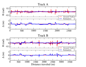
Figure 6: Dynamic performance of the lateral VPC-CILQR algorithm and MTUNet$\_$1$\times$ model for an ego vehicle with heading $\theta$ and lateral offset $\Delta$ for lane-keeping maneuver in the central lane of Track A and B at 76 and 50 km/h, respectively. At the curviest section of Track A (near 1900 m), the maximal $\Delta$ value is 0.52 m; the ego car controlled by this model outperformed the ego car controlled by the Stanley controller (Fig. 3 in [30]), MTL-RL [Fig. 11 (a) in [33]], or CILQR (Fig. 7) algorithms.

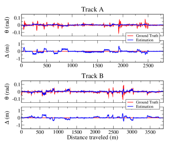
Figure 7: Dynamic performance of the lateral CILQR algorithm and MTUNet$\_$1$\times$ model for the lane-keeping maneuver in the central lane of Track A and B at the same speeds as in Fig. 6. At the curviest section of Track A (near 1900 m), the maximal $\Delta$ value is 0.71 m, which is 1.36 times larger than that of the ego car controlled by the VPC-CILQR algorithm.

TABLE VIII: Performance of VPC-CILQR, CILQR, VPC-SQP, and SQP algorithms with MTUNet$\_$1$\times$ in terms of the mean absolute error (MAE) of parameters presented in Figs. 6-10

	VPC-CILQR		CILQR		VPC-SQP		SQP
(lateral dir.)	$\theta$ (rad)	$\Delta$ (m)	$\theta$ (rad)	$\Delta$ (m)	$\theta$ (rad)	$\Delta$ (m)	$\theta$ (rad)	$\Delta$ (m)
Track A	0.0086	0.0980	0.0083	0.1058	0.0122	0.1071	0.0118	0.1187
Track B	0.0079	0.0748	0.0074	0.0775	0.0099	0.1286	0.0121	0.1470
(longitudinal dir.)	$v$ (m/s)	$D$ (m)	$v$ (m/s)	$D$ (m)	$v$ (m/s)	$D$ (m)	$v$ (m/s)	$D$ (m)
Track Ba	-	-	0.1971	0.4201	-	-	0.2629	0.4930
aComputation from 1150 to 1550 m

To objectively evaluate the dynamic performance of autonomous driving algorithms, lane-keeping and car-following maneuvers were performed on the challenging Tracks A and B shown in Fig. 4. We implemented SQP-based controllers using the ACADO toolkit [70] to conduct comparisons with the CILQR-based controllers. The settings of these algorithms were the same, and the relevant parameters are summarized in Table VII. For lateral control experiments, autonomous vehicles were designed to drive at cruise speeds of 76 and 50 km/h on Track A and B, respectively. The validation results of the VPC-CILQR, CILQR, VPC-SQP, and SQP algorithms for $\theta$ and $\Delta$ are presented in Figs. 6, 7, 8, and 9, respectively. All methods including the MTUNet$\_$1$\times$ model could guide the ego car such that it drove along the lane center and completed one lap on Tracks A and B. The discrepancy in the heading $\theta$ between the MTUNet$\_$1$\times$ estimation and the ground truth trajectory was attributable to curvy or shadowy road segments, which may induce vehicle jittering (see the $\theta$ data for Track A in Figs. 6-9) [33]. Nevertheless, the $\Delta$ values estimated from lane line segmentation results were more robust in difficult scenarios than those obtained using the end-to-end method [67]. Therefore, $\Delta$ can help controllers effectively correct $\theta$ errors and return the ego car to the road’s center (see the $\Delta$ data for Track A in Figs. 6-9). The maximum $\Delta$ deviations from the ideal zero values on Track A for the ego car controlled by the VPC-CILQR controller (shown in Fig. 6) were smaller than those for the cars controlled by the CILQR [21] (Fig. 7) or MTL-RL [33] algorithms. This finding indicates that for curvy roads, the VPC-CILQR algorithm better minimized $\Delta$ than did the other investigated algorithms. Due to the lower computation efficiency (slower reaction time) of the standard SQP solver [21], the VPC-SQP and SQP algorithms had worse performance than the CILQR-based algorithms on the curviest sections of Track A and B (Figs. 8 and 9); however, the VPC-SQP algorithm achieved better performance than the SQP algorithm demonstrating the effectiveness of the VPC algorithm. The resulting mean absolute errors (MAEs) of $\theta$ and $\Delta$ in Figs. 6-9 are listed in the first row of Table VIII; the VPC-CILQR controller outperformed the other methods in terms of $\Delta$-MAE on both tracks. However, the $\theta$-MAE of the VPC-CILQR controller was 0.0003 and 0.0005 rad higher than that of the CILQR controller on Track A and B, respectively. This may have been because the optimality of CILQR solution is losing if the external VPC algorithm is applied to it. This problem could be solved by applying standard MPC methods with more general lane-keeping dynamics, such as the lateral control model presented in [57], which uses road curvature to describe vehicle states. This nonlinear MPC design is computationally expensive and may not meet the requirements for real-time autonomous driving.

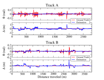
Figure 8: Dynamic performance of the lateral VPC-SQP algorithm and MTUNet$\_$1$\times$ model for the lane-keeping maneuver in the central lane of Track A and B at the same speed as that in Fig. 6. Regarding the curviest section of Track A and B (near 1900 and 2750 m, respectively), the performance of the VPC-SQP algorithm is inferior to that of the VPC-CILQR and CILQR algorithms (Figs. 6 and 7), which outperform the SQP algorithm (Fig. 9), demonstrating the effectiveness of the VPC algorithm.

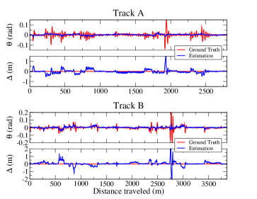
Figure 9: Dynamic performance of the lateral SQP algorithm and MTUNet$\_$1$\times$ model for the lane-keeping maneuver in the central lane of Track A and B at the same speed as that in Fig. 6. The model performance at the curviest section of Track A and B (near 1900 and 2750 m, respectively) is worse than that of all other tested methods.

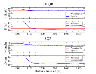
Figure 10: Experiment results of longitudinal CILQR and SQP algorithms in car-following scenario after ego car travels 1075 m on Track B; $v$ and $D$ are speed and inter-vehicle distance, respectively.

Fig. 10 presents the longitudinal experimental results for the CILQR and SQP controllers. The maneuver was performed on a section of Track B; the ego vehicle was initially cruising at 76 km/h and approached a slower preceding car with speed in the range of 63 to 64 km/h. For all ego vehicles under CILQR/SQP control, speed could be regulated, the preceding vehicle could be tracked, and a safe distance between vehicles could be maintained. However, the uncertainty in the optimal solution led to differences between the reference and response trajectories [18]. For the longitudinal CILQR and SQP controllers, respectively, the $v$-MAE was 0.1971 and 0.2629 m/s and $D$-MAE was 0.4201 and 0.4930 m (second row of Table VIII). Hence, CILQR again outperformed SQP in this experiment. Table IX presents the average time to arrive at a solution for the VPC, CILQR, and SQP algorithms. The computation period of VPC was shorter than the MTUNet$\_$1$\times$ inference time (24.52 ms); the iterative periods of the CILQR/SQP solvers were shorter/longer than the ego vehicle control period (6.66 ms), and the SQP solvers required 16.7 and 21.5 times more computation time per cycle than did the CILQR solvers to accomplish the lane-keeping and car-following tasks, respectively. A supplementary video featuring the lane-keeping and car-following simulations can be found at https://youtu.be/Un-IJtCw83Q.

TABLE IX: Average computation time of VPC, CILQR, and SQP algorithms

	VPC	CILQR	SQP
Lateral dir.	15.56 ms	0.58 ms	9.70 ms
Longitudinal dir.	-	0.65 ms	14.01 ms

V Conclusion

In this paper, we propose a vision-based self-driving system that uses a monocular camera and radars to collect sensing data; the system comprises an MTUNet network for environment perception and VPC and CILQR modules for motion planning. The proposed MTUNet model is an improvement on our previous model [30]; we have added a YOLOv4 detector and increased the network’s efficiency by reducing the network input size for use with TORCS [30], CULane [61], and LLAMAS [62] data. The most efficient MTUNet model, namely MTUNet$\_$1$\times$, achieved an inference speed of 40.77 FPS for simultaneous lane line segmentation, ego vehicle pose estimation, and traffic object detection tasks. For vehicular automation, a lateral VPC-CILQR controller was designed that can plan vehicle motion on the basis of the ego vehicle’s heading, lateral offset, and road curvature as determined by MTUNet$\_$1$\times$ and post-processing methods. The longitudinal CILQR controller is activated when a slower preceding car is detected. The optimal jerk is then applied to regulate the ego vehicle’s speed to prevent a collision. The MTUNet$\_$1$\times$ and VPC-CILQR controller can collaborate for ego vehicle operation on challenging tracks in TORCS; this algorithm outperforms methods based on CILQR [21] or MTL-RL [33] algorithms for the same path-tracking task on the same large-curvature roads. The present experiments validated the applicability and demonstrated the feasibility of the proposed system, which comprises perception, planning, and control algorithms and is suitable for real-time autonomous vehicle applications without requiring HD maps.

References

- [1] S. Grigorescu, B. Trasnea, T. Cocias, and G. Macesanu, “A survey of deep learning techniques for autonomous driving,” J. Field Robot, vol. 37, pp. 362-386, 2020.
- [2] E. Yurtsever, J. Lambert, A. Carballo and K. Takeda, “A Survey of Autonomous Driving: Common Practices and Emerging Technologies,” IEEE Access, vol. 8, pp. 58443-58469, 2020.
- [3] A. Tampuu, T. Matiisen, M. Semikin, D. Fishman and N. Muhammad, “A Survey of End-to-End Driving: Architectures and Training Methods,” IEEE Trans. Neural Netw. Learn. Syst., vol. 33, no. 4, pp. 1364-1384, April 2022.
- [4] Y. Li and J. Ibanez-Guzman, “Lidar for Autonomous Driving: The Principles, Challenges, and Trends for Automotive Lidar and Perception Systems,” IEEE Signal Process. Mag., vol. 37, no. 4, pp. 50-61, July 2020.
- [5] “Active Driving Assistance Systems: Test Results and Design Recommendations,” Consumer Reports, Nov 2020.
- [6] M. Teichmann, M. Weber, M. Zöllner, R. Cipolla and R. Urtasun, “MultiNet: Real-time Joint Semantic Reasoning for Autonomous Driving,” in IEEE Intelligent Vehicles Symposium (IV), 2018, pp. 1013-1020.
- [7] F. Pizzati and F. García, “Enhanced free space detection in multiple lanes based on single CNN with scene identification,” in IEEE Intelligent Vehicles Symposium (IV), 2019, pp. 2536-2541.
- [8] Y. Qian, J. M. Dolan and M. Yang, “DLT-Net: Joint Detection of Drivable Areas, Lane Lines, and Traffic Objects,” IEEE Trans. Intell. Transp. Syst., vol. 21, no. 11, pp. 4670-4679, Nov. 2020.
- [9] C.-Y. Lai, B.-X. Wu, V. M. Shivanna and J.-I. Guo, “MTSAN: Multi-Task Semantic Attention Network for ADAS Applications,” IEEE Access, vol. 9, pp. 50700-50714, 2021.
- [10] D. Wu, M. Liao, W. Zhang, X. Wang, X. Bai, W. Cheng, W. Liu, “YOLOP: You Only Look Once for Panoptic Driving Perception,” Mach. Intell. Res., vol. 19, pp. 550–562, 2022.
- [11] “Artificial Intelligence & Autopilot,” www.tesla.com/AI. https://www.tesla.com/AI (accessed May. 21, 2023).
- [12] B. Paden, M. Čáp, S. Z. Yong, D. Yershov and E. Frazzoli, “A Survey of Motion Planning and Control Techniques for Self-Driving Urban Vehicles,” IEEE Trans. Intell. Veh., vol. 1, no. 1, pp. 33-55, March 2016.
- [13] W. Lim, S. Lee, M. Sunwoo and K. Jo, “Hybrid Trajectory Planning for Autonomous Driving in On-Road Dynamic Scenarios,” IEEE Trans. Intell. Transp. Syst., vol. 22, no. 1, pp. 341-355, Jan. 2021.
- [14] B. Gutjahr, L. Gröll and M. Werling, “Lateral Vehicle Trajectory Optimization Using Constrained Linear Time-Varying MPC,” IEEE Trans. Intell. Transp. Syst., vol. 18, no. 6, pp. 1586-1595, June 2017.
- [15] V. Turri, A. Carvalho, H. E. Tseng, K. H. Johansson and F. Borrelli, “Linear model predictive control for lane keeping and obstacle avoidance on low curvature roads,” in 16th International IEEE Conference on Intelligent Transportation Systems (ITSC 2013), 2013, pp. 378-383.
- [16] A. Katriniok, J. P. Maschuw, F. Christen, L. Eckstein and D. Abel, “Optimal vehicle dynamics control for combined longitudinal and lateral autonomous vehicle guidance,” in European Control Conference (ECC), 2013, pp. 974-979.
- [17] S. E. Li, Z. Jia, K. Li and B. Cheng, “Fast Online Computation of a Model Predictive Controller and Its Application to Fuel Economy–Oriented Adaptive Cruise Control,” IEEE Trans. Intell. Transp. Syst., vol. 16, no. 3, pp. 1199-1209, June 2015.
- [18] W. Lim, S. Lee, J. Yang, M. Sunwoo, Y. Na and K. Jo, “Automatic Weight Determination in Model Predictive Control for Personalized Car-Following Control,” IEEE Access, vol. 10, pp. 19812-19824, 2022.
- [19] J. Mattingley and S. Boyd, “CVXGEN: A code generator for embedded convex optimization,” Optim. Eng., vol. 13, no. 1, pp. 1-27, 2012.
- [20] J. Chen, W. Zhan and M. Tomizuka, “Constrained iterative LQR for on-road autonomous driving motion planning,” in IEEE 20th International Conference on Intelligent Transportation Systems (ITSC), 2017, pp. 1-7.
- [21] J. Chen, W. Zhan and M. Tomizuka, “Autonomous Driving Motion Planning With Constrained Iterative LQR,” IEEE Trans. Intell. Veh., vol. 4, no. 2, pp. 244-254, June 2019.
- [22] D. H. Jacobson and D. Q. Mayne, Differential Dynamic Programming. New York, USA: Elsevier, 1970.
- [23] Y. Pan, Q. Lin, H. Shah and J. M. Dolan, “Safe Planning for Self-Driving Via Adaptive Constrained ILQR,” in IEEE/RSJ International Conference on Intelligent Robots and Systems (IROS), 2020, pp. 2377-2383.
- [24] O. Jahanmahin, Q. Lin, Y. Pan and J. M. Dolan, “Jerk-Minimized CILQR for Human-Like Driving on Two-Lane Roadway,” in IEEE Intelligent Vehicles Symposium (IV), 2021, pp. 1282-1289.
- [25] J. Ma, Z. Cheng, X. Zhang, Z. Lin, F. L. Lewis and T. H. Lee, “Local Learning Enabled Iterative Linear Quadratic Regulator for Constrained Trajectory Planning,” IEEE Trans. Neural Netw. Learn. Syst., vol. 34, no. 9, pp. 5354-5365, Sept. 2023.
- [26] M. Werling, J. Ziegler, S. Kammel, and S. Thrun, Optimal trajectory generation for dynamic street scenarios in a Frenét frame, in: IEEE International Conference on Robotics and Automation (ICRA), 2010, pp. 987-993.
- [27] H. Fan, F. Zhu, C. Liu, L. Zhang, L. Zhuang, D. Li, W. Zhu, J. Hu, H. Li, Q. Kong, “Baidu Apollo EM Motion Planner,” 2018, arXiv:1807.08048. [Online]. Available: https://arxiv.org/abs/1807.08048
- [28] K. Lee, S. Jeon, H. Kim and D. Kum, “Optimal Path Tracking Control of Autonomous Vehicle: Adaptive Full-State Linear Quadratic Gaussian (LQG) Control,” IEEE Access, vol. 7, pp. 109120-109133, 2019.
- [29] D.-H. Lee, K.-L. Chen, K.-H. Liou, C.-L. Liu, and J.-L. Liu, “Deep learning and control algorithms of direct perception for autonomous driving,” Appl. Intell. vol. 51, pp. 237-247, 2021.
- [30] D.-H. Lee, C.-L. Liu, “Multi-task UNet architecture for end-to-end autonomous driving”, 2021, arXiv:2112.08967. [Online]. Available: https://arxiv.org/abs/2112.08967
- [31] D.-H. Lee, C.-L. Liu, “End-to-end deep learning of lane detection and path prediction for real-time autonomous driving,” Signal, Image and Video Processing, vol. 17, pp. 199–205, 2023.
- [32] S. Thrun et al., “Stanley: The robot that won the DARPA grand challenge,” J. Field Robot, vol. 23, pp. 661-692, 2006.
- [33] D. Li, D. Zhao, Q. Zhang, and Y. Chen, “Reinforcement learning and deep learning based lateral control for autonomous driving,” IEEE Comput. Intell. Mag. vol. 14, no. 2, pp. 83-98, May 2019.
- [34] J. Liu, Z. Yang, Z. Huang, W. Li, S. Dang and H. Li, “Simulation Performance Evaluation of Pure Pursuit, Stanley, LQR, MPC Controller for Autonomous Vehicles,” in IEEE International Conference on Real-time Computing and Robotics (RCAR), 2021, pp. 1444-1449.
- [35] P. Lu, C. Cui, S. Xu, H. Peng and F. Wang, “SUPER: A Novel Lane Detection System,” IEEE Trans. Intell. Veh., vol. 6, no. 3, pp. 583-593, Sept. 2021.
- [36] A. Bochkovskiy, C.-Y. Wang, H.-Y. M. Liao, “YOLOv4: Optimal Speed and Accuracy of Object Detection,” 2020, arXiv:2004.10934. [Online]. Available: https://arxiv.org/abs/2004.10934
- [37] J. -M. Georg, J. Feiler, S. Hoffmann and F. Diermeyer, ”Sensor and Actuator Latency during Teleoperation of Automated Vehicles,” in IEEE Intelligent Vehicles Symposium (IV), 2020, pp. 760-766.
- [38] J. Betz et al., “TUM autonomous motorsport: An autonomous racing software for the Indy Autonomous Challenge,” J. Field Robot, vol. 40, pp. 783–809, 2023.
- [39] Y. Su, K. K. Tan, and T. H. Lee, “Computation delay compensation for real time implementation of robust model predictive control,” J. of Process Control, vol. 23, pp. 1342-1349, 2013.
- [40] N. Ibtehaz, M. S. Rahman, “MultiResUNet: Rethinking the U-Net architecture for multimodal biomedical image segmentation,” Neural Networks, vol. 121, pp. 74-87, 2020.
- [41] K. Simonyan, A. Zisserman, “Very Deep Convolutional Networks for Large-Scale Image Recognition,” in International Conference on Learning Representations (ICLR), 2015, pp. 1-14.
- [42] O. Ronneberger, P. Fischer, and T. Brox, “U-Net: Convolutional networks for biomedical image segmentation,” in International Conference on Medical Image Computing and Computer-Assisted Intervention (MICCAI), Springer, 2015, pp. 234-241.
- [43] T. Bruls, W. Maddern, A. A. Morye, and P. Newman, “Mark yourself: Road marking segmentation via weakly-supervised annotations from multimodal data,” in IEEE International Conference on Robotics and Automation (ICRA), 2018, pp. 1863-1870.
- [44] S. Xie and Z. Tu, “Holistically-nested edge detection,” in IEEE International Conference on Computer Vision (ICCV), 2015, pp. 1395-1403.
- [45] Q. Zou, H. Jiang, Q. Dai, Y. Yue, L. Chen and Q. Wang, “Robust lane detection from continuous driving scenes using deep neural networks,” IEEE Trans. Veh. Technol, vol. 69, no. 1, pp. 41-54, Jan. 2020.
- [46] H. Cui, V. Radosavljevic, F.-C. Chou, T.-H. Lin, T. Nguyen, T.-K. Huang, J. Schneider, and N. Djuric, “Multimodal trajectory predictions for autonomous driving using deep convolutional networks,” in International Conference on Robotics and Automation (ICRA), 2019, pp. 2090-2096.
- [47] Z. Zheng, P. Wang, W. Liu, J. Li, R. Ye, and D. Ren. “Distance-IoU Loss: Faster and better learning for bounding box regression,” in Proceedings of the AAAI Conference on Artificial Intelligence (AAAI), 2020, vol. 34, no. 7, pp. 12993-13000.
- [48] C. Guo, X.‑l. Lv, Y. Zhang, M.‑l. Zhang, “Improved YOLOv4-tiny network for real-time electronic component detection,” Sci Rep, vol. 11, pp. 22744, 2021.
- [49] J. I. Choi and Q. Tian, “Adversarial Attack and Defense of YOLO Detectors in Autonomous Driving Scenarios,” in IEEE Intelligent Vehicles Symposium (IV), 2022, pp. 1011-1017.
- [50] Y. Tassa, T. Erez and E. Todorov, “Synthesis and stabilization of complex behaviors through online trajectory optimization,” in IEEE/RSJ International Conference on Intelligent Robots and Systems, 2012, pp. 4906-4913.
- [51] Y. Tassa, N. Mansard and E. Todorov, “Control-limited differential dynamic programming,” in IEEE International Conference on Robotics and Automation (ICRA), 2014, pp. 1168-1175.
- [52] B. Plancher, Z. Manchester and S. Kuindersma, “Constrained unscented dynamic programming,” in IEEE/RSJ International Conference on Intelligent Robots and Systems (IROS), 2017, pp. 5674-5680.
- [53] C. V. Samak, T. V. Samak, and S. Kandhasamy, “Control Strategies for Autonomous Vehicles,” 2021, arXiv:2011.08729. [Online]. Available: https://arxiv.org/abs/2011.08729
- [54] W. Qiu, Q. Ting, Y. Shuyou, G. Hongyan, and C. Hong, “Autonomous vehicle longitudinal following control based on model predictive control,” in 34th Chinese Control Conference (CCC), IEEE, 2015, pp. 8126-8131.
- [55] B. Huval et al., “An Empirical Evaluation of Deep Learning on Highway Driving,” 2015, arXiv:1504.01716. [Online]. Available: https://arxiv.org/abs/1504.01716
- [56] X. Zhang and X. Zhu, “Autonomous path tracking control of intelligent electric vehicles based on lane detection and optimal preview method,” Expert Syst. Appl., vol. 121, pp. 38-48, 2019.
- [57] S. Xu, H. Peng, P. Lu, M. Zhu and Y. Tang, “Design and Experiments of Safeguard Protected Preview Lane Keeping Control for Autonomous Vehicles,” IEEE Access, vol. 8, pp. 29944-29953, 2020.
- [58] W. Liu, D. Anguelov, D. Erhan, C. Szegedy, S. Reed, C. Fu, and A. Berg, “SSD: Single Shot MultiBox Detector,” in European Conference on Computer Vision (ECCV), 2016, pp. 21-37.
- [59] J. Redmon and A. Farhadi, “YOLO9000: Better, Faster, Stronger,” in IEEE Conference on Computer Vision and Pattern Recognition (CVPR), 2017, pp. 6517-6525.
- [60] S. Lee et al., “VPGNet: Vanishing Point Guided Network for Lane and Road Marking Detection and Recognition,” in IEEE International Conference on Computer Vision (ICCV), 2017, pp. 1965-1973.
- [61] X. Pan, J. Shi, P. Luo, X. Wang, and X. Tang. “Spatial as deep: spatial CNN for traffic scene understanding,” in The Thirty-Second AAAI Conference on Artificial Intelligence (AAAI-18), 2018, no. 891, pp. 7276–7283.
- [62] K. Behrendt, R. Soussan, “Unsupervised Labeled Lane Markers Using Maps,” in IEEE/CVF International Conference on Computer Vision Workshop (ICCVW), 2019, pp. 832-839.
- [63] J. MacQueen et al., “Some methods for classification and analysis of multivariate observations,” in Proceedings of the fifth Berkeley symposium on mathematical statistics and probability, 1967, pp. 281–297.
- [64] S. Liang et al., “Edge YOLO: Real-Time Intelligent Object Detection System Based on Edge-Cloud Cooperation in Autonomous Vehicles,” IEEE Trans. Intell. Transp. Syst., vol. 23, no. 12, pp. 25345-25360, Dec. 2022.
- [65] W. Bernhard et al., “TORCS: The open racing car simulator,” 2014. [Online]. Available: http://www.torcs.org
- [66] K. Fitzpatrick, “Horizontal Curve Design: An Exercise in Comfort and Appearance,” Transp. Res. Rec., vol. 1445 pp. 47-53, 1994.
- [67] C. Chen, A. Seff, A. Kornhauser, and J. Xiao, “DeepDriving: Learning affordance for direct perception in autonomous driving,” in Proceedings of the IEEE International Conference on Computer Vision, 2015, pp. 2722-2730.
- [68] T. Standley, A. R. Zamir, D. Chen, L. Guibas, J. Malik, and S. Savarese, “Which tasks should be learned together in multi-task learning?” in Proc. 37th Int. Conf. Mach. Learn. (ICML), vol. 119, Jul. 2020, pp. 9120-9132.
- [69] I. Kokkinos, “UberNet: Training a Universal Convolutional Neural Network for Low-, Mid-, and High-Level Vision Using Diverse Datasets and Limited Memory,” in IEEE Conference on Computer Vision and Pattern Recognition (CVPR), 2017, pp. 5454-5463.
- [70] B. Houska, H. J. Ferreau, and M. Diehl, “ACADO toolkit-An open source framework for automatic control and dynamic optimization,” Optim. Control Appl. Methods. vol. 32, no. 3, pp. 298-312, 2011.