Dipole-dipole scattering amplitude in CGC approach

Abstract

In this paper we propose recurrence relations for the dipole densities in QCD, which allows us to find these densities from the solution to the BFKL equation. We resolve these relations in the diffusion approximation for the BFKL kernel. Based on this solution, we found the sum of large Pomeron loops. This sum generates the scattering amplitude that decreases at large values of rapidity $Y$. It turns out that such behaviour of the scattering amplitudes is an artifact of diffusion approximation. This approximation leads to the unitarization without saturation both in deep inelastic scattering and in dipole-dipole interaction at high energies.

I Introduction

The main ideas of Colour Glass Condensate(CGC)/saturation approach (see Ref.KOLEB for a review) : the saturation of the dipole density and the new dimensional scale ($Q_{s}$), which increases with energy, have become the common language for discussing the high energy scattering in QCD. However, in spite of intensive work BFKL ; LIP ; LIREV ; LIFT ; GLR ; GLR1 ; MUQI ; MUDI ; MUSA ; Salam ; NAPE ; BART ; BKP ; MV ; KOLE ; BRN ; BRAUN ; BK ; KOLU ; JIMWLK1 ; JIMWLK2 ; JIMWLK3 ; JIMWLK4 ; JIMWLK5 ; JIMWLK6 ; JIMWLK7 ; JIMWLK8 ; AKLL ; KOLU1 ; KOLUD ; BA05 ; SMITH ; KLW ; KLLL1 ; KLLL2 , we have several problems, that have not been solved. One of the principle problems is summing Pomeron loops, without solving which we cannot consider the dilute-dilute and dense-dense parton densities collisions. As has been recently shownKLLL1 ; KLLL2 , even the Balitsky-Kovchegov (BK) equation, that governs the dilute-dense parton density scattering (deep inelastic scattering (DIS) of electron with proton), has to be modified due to contributions of Pomeron loops.

In this paper we attempt to sum Pomeron loops for dipole-dipole scattering amplitude at high energies. This attempt is based on the experience with the simple, but exactly solvable, two dimensional modelsMUSA ; ACJ ; AAJ ; JEN ; ABMC ; CLR ; CIAF ; BIT ; RS ; KLremark2 ; SHXI ; KOLEV ; nestor ; LEPRI ; utm ; utmm , which we will discuss in the next section. From these models we learned, that the scattering amplitude at high energies is determined by the sum of large Pomeron loops. Actually, the formalism for summing large Pomeron loops in QCD has been developed MUSA ; IAMU ; IAMU1 ; LELU ; KO1 ; LE1 . In this paper, we propose new recurrence relations for the parton densities in QCD, which allows us to find all parton densities from the solution of the BFKL equation. We resolve these recurrence relations in the diffusion approximation for the BFKL kernel and suggest the explicit form for the scattering amplitude. We believe that we have completed the approach which was started in Refs.KO1 ; LE1 .

II Pomeron calculus in zero transverse dimension-a recap

The simple toy model: the Pomeron calculus in zero transverse dimension, is a respectable tool and a well known training ground for the interaction at high energiesACJ ; AAJ ; JEN ; ABMC ; CLR ; CIAF ; MUSA ; Salam ; RS ; KLremark2 ; SHXI ; KOLEV ; BIT ; nestor ; LEPRI ; utm ; utmm . Due to the simplicity of these models, we are able to formulate and solve the reggeon field theory (RFT) for the interacting Pomerons. This theory satisfies both the $s$ and $t$ channel unitarity constraints and includes the emission of the dipoles as well as the saturation effects in the corresponding parton cascades. The simple toy model also gives examples of theories that have the probabilistic interpretation for the scattering amplitude in letter and spirit of the partonic approach.

In Ref.MUSA the simple probabilistic formula for the S-matrix is suggested:

$$S(Y)\,\,=\,\,\sum_{n,m}e^{-m\,n\,\gamma}\,P^{\mbox{\tiny BFKL}}_{n}(Y_{0})\,P^{\mbox{\tiny BFKL}}_{m}(Y-Y_{0})$$ (1)

where $\gamma$ is the scattering amplitude of two dipoles and $P^{\mbox{\tiny BFKL}}_{n}(Y)$ is the probability distribution in the BFKL cascade For $P_{n}(Y)$ we have equations in the following form for the zero transverse dimension:

$$\frac{d\,P^{\mbox{\tiny BFKL}}_{n}(Y)}{d\,Y}\,\,=\,\,-\Delta\,n\,P^{\mbox{\tiny BFKL}}_{n}(Y)\,\,+\,\,\Delta\,(n-1)\,P^{\mbox{\tiny BFKL}}_{n-1}(Y)$$ (2)

with the solution:

$$P_{n}^{BK}(Y)=\frac{1}{N(Y)-1}\left(1-\frac{1}{N(Y)}\right)^{n}\,\,\,\xrightarrow{Y\,\gg\,1}\,\,\,\frac{1}{N(Y)}\exp\left(-\frac{n}{N(Y)}\right)$$ (3)

where $N(Y)$ is the first factorial moment or multiplicity of dipoles: $N(Y)=e^{\Delta\,Y}$. Generally speaking Eq. (1) does depend on the reference frame (on the value of $Y_{0}$) and, as has been discussed in Refs.MUSA ; BIT ; utm ; utmm , we need to change Eq. (2) to obtain the Pomeron calculus which satisfies both $t$ and $s$ channel unitarity. However, at large values of $Y-Y_{0}$ and $Y_{0}$ Eq. (1) leads to the scattering amplitude that does not depend on the value of $Y_{0}$utmm . Indeed,

$$S(Y) = \sum_{n,m}e^{-m\,n\,\gamma}\,P^{\mbox{\tiny BFKL}}_{n}(Y_{0})\,P^{\mbox{\tiny BFKL}}_{m}(Y-Y_{0})\,\,=\,\,\sum_{k=0}^{\infty}\frac{\left(-\gamma\right)^{k}}{k!}\underbrace{\Bigg{(}\sum_{n=0}^{\infty}n^{k}\,P_{n}(Y_{0})\Bigg{)}}_{c_{k}\left(Y_{0}\right)}\underbrace{\Bigg{(}\sum_{m=0}^{\infty}m^{k}\,P_{m}(Y-Y_{0})\Bigg{)}}_{c_{k}\left(Y-Y_{0}\right)}\,\,$$ (4)

$$= \sum_{k=0}^{\infty}\,(-\gamma N\left(Y_{0}\right)\,N\left(Y-Y_{0}\right))^{k}\,k!\,=\,\sum_{k=0}^{\infty}\,(-\gamma N\left(Y\right))^{k}\,k!=\,-\frac{e^{\frac{1}{\gamma N(Y)}}\text{Ei}\left(-\frac{1}{N(Y)\gamma}\right)}{\gamma N(Y)}$$

In Eq. (4) we used that (1) $N\left(Y-Y_{0}\right)\,N\left(Y_{0}\right)=N\left(Y\right)$; and (2) the factorial moments of the distribution of Eq. (3) has the following form

$$M_{k}(Y)\,\,=\,\,k!N(Y)\left(N(Y)\,-\,1\right)^{k-1}\,\,\xrightarrow{N(Y)\,\gg\,1}\,\,\,c_{k}(Y)=k!N^{k}(Y)$$ (5)

One can see that $S(Y)$, being a function of $N(Y)$, does not depend on the reference frame. It turns out that this S-matrix at large $Y-Y_{0}$ and $Y_{0}$ coincides with the one calculated in the UTMMUSA ; utm ; utmm : theory, which is independent of a reference frame at any value of $Y_{0}$ .

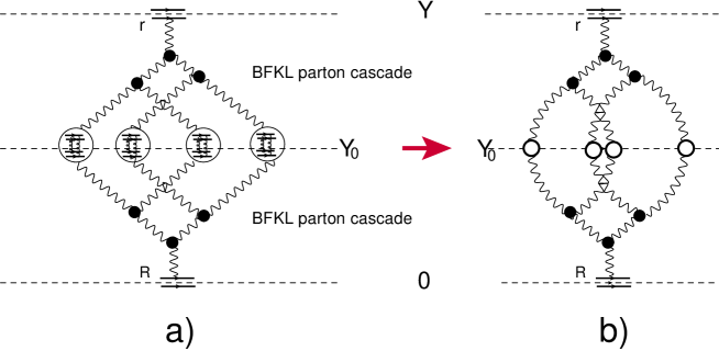
Figure 1: Summing large Pomeron loops. The wavy lines denote the BFKL Pomeron exchanges in Fig. 1-a and in Fig. 1-b the Pomeron in the two dimensional Pomeron calculus with the Green’s function $G_{I\!\!P}(Y)=\exp\left(\Delta\,Y\right)$. The black circles stand for the triple Pomeron vertices in both figures, which are equal to $\Delta$ In Fig. 1-b, while the white circles denote the amplitude $\gamma$. In Fig. 1-a we show the dipole-dipole scattering amplitude in the Born approximation of perturbative QCD in the circles.

It is easy to see that the S-matrix of Eq. (1) sums the large BFKL Pomeron loops shown in Fig. 1. Indeed, the contribution of large Pomeron loops can be written in the following form:MUDI ; IAMU ; LELU ; KO1 ; LE1 :

$$S(Y)\,\, = \,\,\sum_{n}\frac{(-\,\gamma)^{n}}{n!}M_{n}\left(Y-Y_{0}\right)\,M_{n}\left(Y_{0}\right)\,\,\,\xrightarrow{Y-Y_{0},Y_{0}\gg 1}\sum_{n}(-\,\gamma)^{n}\,n!\left(N\left(Y-Y_{0}\right)\,N\left(Y_{0}\right)\right)^{n}$$ (6)

$$= \,\,\sum_{n}(-\,\gamma)^{n}\,n!\left(G_{I\!\!P}\left(Y-Y_{0}\right)\,G_{I\!\!P}\left(Y_{0}\right)\right)^{n}=-\frac{e^{\frac{1}{\gamma N(Y)}}\text{Ei}\left(-\frac{1}{N(Y)\gamma}\right)}{\gamma N(Y)}$$

$M_{n}$ in Eq. (6) are the factorial moments which we replace by $M_{n}(Y)\,=\,n!N^{n}\left(Y\right)$ at large $Y$ for distribution of Eq. (3). In Eq. (6) $N\left(Y\right)=N\left(Y-Y_{0}\right)\,N\left(Y_{0}\right)$. The advantage of this derivation is that it can be easily generalize to the QCD case, which is the main goal of this paper.

The factorial moments will play an essential role in our approach. Bearing this in mind, we wish to write the equation for them in the simple BFKL cascade of Eq. (2). The solution of Eq. (3) it is easy to obtain introducing the generating function:

$$Z\left(Y,u\right)\,\,=\,\,\sum_{n=1}^{\infty}\,P_{n}\left(Y\right)\,u^{n}$$ (7)

One can see that

$$P_{n}\left(Y\right)\,\,=\,\,\frac{1}{n!}\frac{\partial\,Z\left(Y,u\right)}{\partial u^{n}}\Big{|}_{u=0};~{}~{}~{}M_{n}\left(Y\right)\,\,=\,\,\sum_{n}\left(n(n-1)\dots(n-k+1)\right)\,P_{n}(Y)=\frac{\partial\,Z\left(Y,u\right)}{\partial u^{n}}\Big{|}_{u=1};$$ (8)

From Eq. (2) the equation for $Z$ takes the form:

$$\frac{\partial\,Z\left(Y,u\right)}{\partial\,Y}\,\,=\,\,-\Delta\,u(1-u)\frac{\partial\,Z\left(Y,u\right)}{\partial\,u}$$ (9)

Taking $n$-derivatives from Eq. (9) and substituting $u=1$ we obtain the following equation for $M_{n}(Y)$;

$$\frac{\partial\,M_{n}\left(Y\right)}{\partial\,Y}\,\,=\,\,\Delta\,n\,\,M_{n}\left(Y\right)\,\,+\,\Delta\,n(n-1)M_{n-1}\left(Y\right)$$ (10)

Eq. (10) has a more elegant form for $\rho_{n}(Y)\,\,=\,\,M_{n}(Y)/n!$:

$$\frac{\partial\,\rho_{n}\left(Y\right)}{\partial\,Y}\,\,=\,\,\Delta\,n\,\,\rho_{n}\left(Y\right)\,\,+\,\Delta\,(n-1)\rho_{n-1}\left(Y\right)$$ (11)

For sum of the large Pomeron loops we have the following formula, using $\rho_{n}(Y)$:

$$S(Y)\,\,=\,\,\sum_{n}(-\,\gamma)^{n}\,n!\,\rho_{n}\left(Y-Y_{0}\right)\,\rho_{n}\left(Y_{0}\right)$$ (12)

Eq. (12) has been generalized to the QCD case in Refs.IAMU ; LELU and we will use it in our approach.

Eq. (9) for the generating function $Z$ can be rewritten as the non-linear equation for $Z$ in the form:

$$\frac{\partial\,Z\left(Y,u\right)}{\partial\,\Delta\,Y}\,\,=\,\,-Z\left(Y,u\right)\Big{(}1\,\,-\,\,Z\left(Y,u\right)\Big{)}$$ (13)

Bearing in mind that $\rho_{n}\left(Y\right)\,\,=\,\,\frac{1}{n!}\frac{\partial\,Z\left(Y,u\right)}{\partial u^{n}}\Big{|}_{u=1}$ we can obtain the equation for $\rho_{n}$ differentiating Eq. (13) and puting $u=1$ :

$$\frac{\partial\,\rho_{n}\left(Y\right)}{\partial\,\Delta\,Y}\,\,=\,\,\rho_{n}\left(Y\right)\,\,+\,\,\sum_{k=1}^{n-1}\rho_{n-k}\left(Y\right)\,\rho_{k}\left(Y\right)$$ (14)

Subtracting this equation from Eq. (11) we obtain the following recurrence relation for $\rho_{n}$:

$$\left(n\,-\,1\right)\,\rho_{n}\left(Y\right)\,\,=\,\,\sum_{k=1}^{n-1}\,\rho_{n-k}\left(Y\right)\,\rho_{k}\left(Y\right)\,\,-\,\,\left(n-1\right)\,\rho_{n-1}\left(Y\right)$$ (15)

Solution to Eq. (15) has the form:

$$\rho_{n}\left(Y\right)\,\,=\,\,\rho_{1}\left(Y\right)\Big{(}\rho_{1}\left(Y\right)\,\,-\,\,1\Big{)}^{n-1}$$ (16)

Summarizing what we have obtained in this section for the simple models of RTF, we conclude that (i) the scattering amplitude at high energies can be calculated from Eq. (12) using the parton densities $\rho_{n}(Y)$; (ii) these parton densities satisfy the two evolution equations of Eq. (11) and Eq. (14); and (iii) these two equations lead to the recurrence relation for $\rho_{n}$ (see Eq. (15). The main goal of this paper is to generalize these ingredients to the case of QCD and obtain the QCD scattering amplitude at high energies.

III Summing large Pomeron loops in QCD

As it has been mentioned, our main goal is to sum large Pomeron loops in QCD to obtain the scattering amplitude. Our approach includes two stages. First, we need to generalize Eq. (12) to the case of QCD. Actually, this problem has been solved in Refs.MUSA ; Salam ; IAMU ; KOLEB ; MUDI ; LELU and we are going to discuss it here. Second, we need to get the evolution equations for the parton densities and find their solutions. This problem has been partly solved in Ref.LELU , but in this section we will find the second evolution equation and suggest the recurrence relations for $\rho_{n}$. Finally, we need to find the solution for the parton densities and this topic is the main one of this section.

III.1 BFKL Parton cascade: evalution equations and recurrence relations for the parton densities

The simple Eq. (2) has been generalized to the QCD case in Refs.KOLEB ; MUDI ; LELU and has the following form :

$$\frac{\partial\,P_{n}\left(Y,\bm{r},\bm{b};\{\bm{r}_{i},\bm{b}_{i}\}\right)}{\partial\,Y}\,=\,-\,\sum^{n}_{i=1}\,\omega_{G}(r_{i})\,P_{n}\left(Y,\bm{r},\bm{b};\,\{\bm{r}_{i},\bm{b}_{i}\},\right)\,\,+\,\,\bar{\alpha}_{S}\,\sum^{n-1}_{i=1}\,\frac{(\bm{r}_{i}\,+\,\bm{r}_{n})^{2}}{(2\,\pi)\,r^{2}_{i}\,r^{2}_{n}}\,P_{n-1}\left(Y,\bm{r},\bm{b};\{\bm{r}_{j},\bm{b}_{j},\bm{r}_{i}+\bm{r}_{n},\bm{b}_{in}\}\right)$$

where $P_{n}\left(Y,r,b;\{r_{i},b_{i}\}\right)$ is the probability to have $n$-dipoles of size $r_{i}$, at impact parameter $b_{i}$ and at rapidity $Y$ . $\bm{b}_{in}$ in Eq. (III.1) is equal to $\bm{b}_{in}\,=\,\bm{b}_{i}\,+\,\frac{1}{2}\bm{r}_{i}\,=\,\bm{b}_{n}\,-\,\frac{1}{2}\bm{r}_{i}$.

Eq. (III.1) is a typical cascade equation in which the first term describes the reduction of the probability to find $n$ dipoles due to the possibility that one of $n$ dipoles can decay into two dipoles of arbitrary sizes , while the second term, describes the growth due to the splitting of $(n-1)$ dipoles into $n$ dipoles. We introduce the generating functionalMUDI

$$Z\left(Y,\bm{r},\bm{b};[u_{i}]\right)\,\,=\,\,\sum^{\infty}_{n=1}\int P_{n}\left(Y,\bm{r},\bm{b};\{\bm{r}_{i}\,\bm{b}_{i}\}\right)\prod^{n}_{i=1}u\left(\bm{r}_{i}\,\bm{b}_{i}\right)\,d^{2}r_{i}\,d^{2}b_{i}$$ (17)

where $u\left(\bm{r}_{i}\,\bm{b}_{i}\right)\equiv\,u_{i}$ is an arbitrary function. The initial and boundary conditions for Eq. (17) take the following form for the functional $Z$:

$$Z\left(Y=0,\bm{r},\bm{b};[u_{i}]\right) \,\,=\,\, u\left(\bm{r},\bm{b}\right);$$ (18a)

$$Z\left(Y,r,[u_{i}=1]\right) = 1;$$ (18b)

Multiplying both parts of Eq. (III.1) by $\prod^{n}_{i=1}u\left(\bm{r}_{i}\,\bm{b}_{i}\right)$ and integrating over $r_{i}$ and $b_{i}$ we obtain the following linear functional equationLELU ;

$$\frac{\partial Z\left(Y,\bm{r},\bm{b};[u_{i}]\right)}{\partial\,Y}=\int d^{2}r^{\prime}\,K\left(\bm{r}^{\prime},\bm{r}-\bm{r^{\prime}}|\bm{r}\right)\Bigg{(}-u\left(r,b\right)\,\,+\,\,u\left(\bm{r}^{\prime},\bm{b}+\frac{1}{2}(\bm{r}-\bm{r}^{\prime})\right)\,u\left(\bm{r}-\bm{r}^{\prime},\bm{b}-\frac{1}{2}\bm{r}^{\prime}\right)\Bigg{)}\frac{\delta\,Z}{\delta\,u\left(r,b\right)};$$ (19a)

$$K\left(\bm{r}^{\prime},\bm{r}-\bm{r^{\prime}}|\bm{r}\right)\,=\frac{\bar{\alpha}_{S}}{2\,\pi}\frac{r^{2}}{r^{\prime 2}\,(\bm{r}-\bm{r}^{\prime})^{2}};\,~{}~{}~{}~{}~{}\omega_{G}\left(r\right)\,\,=\,\,\int d^{2}r^{\prime}K\left(\bm{r}^{\prime},\bm{r}-\bm{r^{\prime}}|\bm{r}\right);$$ (19b)

The $n$-dipole densities $\rho_{n}(r_{1},b_{1},\ldots\,,r_{n},b_{n})$ are defined as followsLELU :

$$\rho_{n}(r_{1},b_{1}\,\ldots\,,r_{n},b_{n};Y\,-\,Y_{0})\,=\,\frac{1}{n!}\,\prod^{n}_{i=1}\,\frac{\delta}{\delta u_{i}}\,Z\left(Y\,-\,Y_{0};\,[u]\right)|_{u=1}$$ (20)

Taking n-th functional derivatives from Eq. (19a) and substituting $u_{1}=1$ we obtain for $\rho_{n}$ LELU :

$$\frac{\partial\,\rho_{n}(\{r_{i},b_{i}\})}{\,\partial\,Y}\,\, = \,\ -\,\sum_{i=1}^{n}\,\,\omega_{G}(r_{i})\,\,\rho_{n}(\{r_{i},b_{i}\})\,\,+\,\,2\,\sum_{i=1}^{n}\,\int\,\frac{d^{2}\,r^{\prime}}{2\,\pi}\,\frac{r^{\prime 2}}{r^{2}_{i}\,(\bm{r}_{i}\,-\,\bm{r}^{\prime})^{2}}\,\rho_{n}(\ldots\,r^{\prime},b_{i}-r^{\prime}/2\dots)$$ (21)

$$\,+\bar{\alpha}_{S}\frac{(\bm{r}_{i}\,+\,\bm{r}_{n})^{2}}{r^{2}_{i}\,\,r^{2}_{n}}\,\sum_{i=1}^{n-1}\rho_{n-1}(\ldots\,(\bm{r}_{i}\,+\,\bm{r}_{n}),b_{in}\dots).$$

Introducing

$$\bar{\rho}_{n}(\bm{r},\bm{b};\{r_{i},b_{i}\})\,=\,\,\prod_{i=1}^{n}\,r^{2}_{i}\,\,\rho_{n}(\{r_{i},b_{i}\})$$ (22)

we reduce Eq. (21) to the following form

$$\frac{\partial\,\bar{\rho}_{n}(\{\bm{r}_{i},\bm{b}_{i}\})}{\,\partial\,Y}\,\, = \,\,\sum_{i=1}^{n}\,\int\,\frac{d^{2}\,r^{\prime}}{2\,\pi}\,K\left(\bm{r}^{\prime},\bm{r}_{i}-\bm{r^{\prime}}|\bm{r}_{i}\right)$$

$$\times \Bigg{\{}\bar{\rho}_{n}(\{\bm{r}_{j},\bm{b}_{j}\},\bm{r}^{\prime},\bm{b}_{i}-(\bm{r}_{i}-\bm{r}^{\prime})/2)\,+\,\bar{\rho}_{n}(\{\bm{r}_{j},\bm{b}_{j}\},\bm{r}_{i}-\bm{r}^{\prime},\bm{b}_{i}-\bm{r}^{\prime}/2)\,-\,\bar{\rho}_{n}(\{\bm{r}_{i},\bm{b}_{i}\})\Bigg{\}}$$

$$\,+\,\bar{\alpha}_{S}\sum_{i=1}^{n-1}\,\bar{\rho}_{n-1}(\ldots\,(\bm{r}_{i}\,+\,\bm{r}_{n}),b_{in}\dots).$$

Eq. (19a) can be rewritten as the non-linear equation for $Z$MUDI ; LELU :

$$\frac{\partial Z\left(Y,\bm{r},\bm{b};[u_{i}]\right)}{\partial\,Y}=\int d^{2}r^{\prime}\,K\left(\bm{r}^{\prime},\bm{r}-\bm{r^{\prime}}|\bm{r}\right)\Bigg{(}-Z\left(Y,\bm{r},\bm{b};[u_{i}]\right)\,\,+\,\,Z\left(\bm{r}^{\prime},\bm{b}+\frac{1}{2}(\bm{r}-\bm{r}^{\prime});[u_{i}]\right)\,Z\left(\bm{r}-\bm{r}^{\prime},\bm{b}-\frac{1}{2}\bm{r}^{\prime};[u_{i}]\right)\Bigg{)}\\$$ (24)

Using the definition of Eq. (20) and differentiating Eq. (24) (see Eq. (20))we obtain a new equation for $\rho_{n}$ :

$$\frac{\partial\,\rho_{n}(\bm{r},\bm{b};\{\bm{r}_{i},\bm{b}_{i}\})}{\,\partial\,Y}\,\,=\,\,\bar{\alpha}_{S}\,\int d^{2}r^{\prime}\,K\left(\bm{r}^{\prime},\bm{r}-\bm{r^{\prime}}|\bm{r}\right)$$

$$\times \,\,\Bigg{\{}\left(\rho_{n}(\bm{r}^{\prime},\bm{b}-\frac{1}{2}(\bm{r}-\bm{r}^{\prime});\{\bm{r}_{i},\bm{b}_{i}\})\,\,+\,\,\rho_{n}(\bm{r}-\bm{r}^{\prime},\bm{b}-\frac{1}{2}\bm{r}^{\prime};\{\bm{r}_{i},\bm{b}_{i}\})-\,\,\rho_{n}(\bm{r},\bm{b};\{\bm{r}_{i},\bm{b}_{i}\})\right)$$

$$+ \bar{\alpha}_{S}\,\,\sum^{n-1}_{k=1}\rho_{n-k}(\bm{r}^{\prime},\bm{b}+\frac{1}{2}(\bm{r}-\bm{r}^{\prime};\{\bm{r}_{i},\bm{b}_{i}\})\,\rho_{k}(\bm{r}-\bm{r}^{\prime},\bm{b}-\frac{1}{2}\bm{r}^{\prime};\{\bm{r}_{i},\bm{b}_{i}\})\Bigg{\}}$$

For $\bar{\rho}_{n}$ it has the same form. This equation together with Eq. (III.1) leads to the recurrence relation for $\bar{\rho}_{n}$, which has the form:

$$\int d^{2}r^{\prime}\,K\left(\bm{r}^{\prime},\bm{r}-\bm{r^{\prime}}|\bm{r}\right)\,\Bigg{\{}\left(\rho_{n}(\bm{r}^{\prime},\bm{b}-\frac{1}{2}(\bm{r}-\bm{r}^{\prime});\{\bm{r}_{i},\bm{b}_{i}\})\,\,+\,\,\rho_{n}(\bm{r}-\bm{r}^{\prime},\bm{b}-\frac{1}{2}\bm{r}^{\prime};\{\bm{r}_{i},\bm{b}_{i}\})-\,\,\rho_{n}(\bm{r},\bm{b};\{\bm{r}_{i},\bm{b}_{i}\})\right)$$ (26)

$$+ \,\sum^{n-1}_{k=1}\rho_{n-k}(\bm{r}^{\prime},\bm{b}+\frac{1}{2}(\bm{r}-\bm{r}^{\prime};\{\bm{r}_{i},\bm{b}_{i}\})\,\rho_{k}(\bm{r}-\bm{r}^{\prime},\bm{b}-\frac{1}{2}\bm{r}^{\prime};\{\bm{r}_{i},\bm{b}_{i}\})\Bigg{\}}\,\,=\,\,\sum_{i=1}^{n}\,\int\,\frac{d^{2}\,r^{\prime}}{2\,\pi}\,K\left(\bm{r}^{\prime},\bm{r}_{i}-\bm{r^{\prime}}|\bm{r}_{i}\right)$$

$$\times \Bigg{\{}\bar{\rho}_{n}(\bm{r},\{\bm{r}_{j},\bm{b}_{j}\},\bm{r}^{\prime},\bm{b}_{i}-(\bm{r}_{i}-\bm{r}^{\prime})/2)\,+\,\bar{\rho}_{n}(\bm{r},\{\bm{r}_{j},\bm{b}_{j}\},\bm{r}_{i}-\bm{r}^{\prime},\bm{b}_{i}-\bm{r}^{\prime}/2)\,-\,\bar{\rho}_{n}(\bm{r},\{\bm{r}_{i},\bm{b}_{i}\})\Bigg{\}}$$

$$+ \,\,\,\sum_{i=1}^{n-1}\,\bar{\rho}_{n-1}(\bm{r},\ldots\,(\bm{r}_{i}\,+\,\bm{r}_{n}),b_{in}\dots)$$

One can see that just from general form of Eq. (III.1) the leading energy behaviour stems from the inhomogeneous term of this equation and we expect that $\bar{\rho}_{n}\,\propto\,\sum^{n-1}_{k}\,\bar{\rho}_{n-k}\,\bar{\rho}_{k}$.

III.2 Main formula

The scattering amplitude shown in Fig. 1-a can be written in the following way LELU ; KO1 ; LE1 :

$$A\left(Y,r,R;\bm{b}\right)\,=\,\sum^{\infty}_{n=1}\,\left(-1\right)^{n+1}\,n!\int\prod\frac{d^{2}r_{i}}{r^{4}_{i}}\,\frac{d^{2}\,r^{\prime}_{i}}{r^{\prime 4}_{i}}\,d^{2}b^{\prime}_{i}\int d^{2}\delta b_{i}\gamma^{BA}\left(r_{1},r^{\prime}_{i},\bm{b}_{i}-\bm{b^{\prime}_{i}}\equiv\delta\bm{b}_{i}\right)\,\,\bar{\rho}\left(Y-Y_{0},\{\bm{r}_{i},\bm{b}_{i}\}\right)\,\bar{\rho}\left(Y_{0},\{\bm{r}^{\prime}_{i},\bm{b}^{\prime}_{i}\}\right)$$ (27)

$\gamma^{BA}$ is the scattering amplitude of two dipoles in the Born approximation of perturbative QCD. Considering $Y-Y_{0}\gg 1$ and $Y_{0}\gg 1$ one can see that the typical $\ln b^{2}_{i}\,\sim\,\sqrt{Y-Y_{0}}$ and $\ln b^{\prime 2}_{i}\,\sim\,\sqrt{Y_{0}}$ are large, while in $\gamma^{BA}$ $\delta b_{i}\,\sim\,r_{1},r^{\prime}_{i}$. Hence, we can neglect the contribution of $\delta b_{i}$ in $\bar{\rho}$. Therefore, in Eq. (27) enters $\int d^{2}\delta b_{i}\gamma^{BA}\left(r_{1},r^{\prime}_{i},\bm{b}_{i}-\bm{b^{\prime}_{i}}\equiv\delta\bm{b}_{i}\right)$ which can be written asMUDI :

$$\sigma^{\rm BA}\left(\bm{r}_{i},\bm{r}^{\prime}_{i}\right)\,\,=\,\,\int d^{2}\delta b_{i}\gamma^{BA}\left(r_{1},r^{\prime}_{i},\bm{b}_{i}-\bm{b^{\prime}_{i}}\equiv\delta\bm{b}_{i}\right)\,\,=\,\,4\,\pi\,\bar{\alpha}_{S}^{2}\int\frac{d\,l}{l^{3}}\,\left(1\,-\,J_{0}\left(l\,r_{i}\right)\right)\,\,\left(1\,-\,J_{0}\left(l\,r^{\prime}_{i}\right)\right)$$ (28)

In Eq. (27) $\bm{b}_{i}\,\,=\,\,\bm{b}\,-\,\bm{b^{\prime}}_{i}$.

III.3 Solutions for $\bar{\rho}_{n}\left(Y,\{r_{i},b_{i}\}\right)$

III.3.1 $\bar{\rho}_{1}\left(Y,r,r_{1},b_{1}\right)$

From Eq. (III.1) for $\bar{\rho}_{1}$ we have the linear equation:

$$\frac{\partial\,\bar{\rho}_{1}(Y;r_{1},b)}{\bar{\alpha}_{S}\,\partial\,Y}\,\,=\,\,-\,\,\omega_{G}\left(r_{1}\right)\bar{\rho}_{1}(Y;r_{1},b)\,\,+\,\,2\,\int\,\frac{d^{2}\,r^{\prime}}{2\,\pi}\,K\left(\bm{r}^{\prime},\bm{r}-\bm{r^{\prime}}|\bm{r}\right)\,\bar{\rho}_{1}\left(Y,r^{\prime},b\right)$$ (29)

The physical meaning of $\rho_{1}$ is clear from Eq. (20): it is the mean number of dipoles with size $r_{1}$ in the partonic wave function of the projectile or target. It is proven in Ref.LIP that the eigenfunction of the BFKL equation has the following form

$$\phi_{\gamma}\left(\bm{r},\bm{r}_{1},\bm{b}_{1}\right)\,\,\,=\,\,\,\left(\frac{r^{2}\,r_{1}^{2}}{\left(\bm{b}_{1}+\frac{1}{2}(\bm{r}-\bm{r}_{1})\right)^{2}\,\left(\bm{b}_{1}-\frac{1}{2}(\bm{r}-\bm{r}_{1})\right)^{2}}\right)^{\gamma}\,\,\xrightarrow{b_{1}\,\gg\,r,r_{1}}\,\,\left(\frac{r^{2}\,r_{1}^{2}}{b_{1}^{4}}\right)^{\gamma}\,\,\equiv\,\,e^{\gamma\,\xi}$$ (30)

for any kernel which satisfies the conformal symmetry. In Eq. (30) $r$ is the size of the initial dipole at $Y=0$ while $r_{1}$ is the size of the dipole with rapidity $Y$. As has been discussed in the previous section, the typical $b_{i}$ in $\bar{\rho}_{n}$ in Eq. (27) is large. Hence we can use the variable $\xi$ from Eq. (30).

For the kernel of the LO BFKL equation (see Eq. (19b)) the eigenvalues take the form:

$$\omega\left(\bar{\alpha}_{S},\gamma\right)\,\,=\,\,\bar{\alpha}_{S}\,\chi\left(\gamma\right)\,\,\,=\,\,\,\bar{\alpha}_{S}\left(2\psi\left(1\right)\,-\,\psi\left(\gamma\right)\,-\,\psi\left(1-\gamma\right)\right)\,\,\xrightarrow{\gamma\,\to\,\frac{1}{2}}\,\underbrace{4\ln 2\bar{\alpha}_{S}}_{\Delta_{\mbox{\tiny{BFKL}}}}\,\,+\,\,\underbrace{14\zeta(3)\bar{\alpha}_{S}}_{D}\left(\gamma-\frac{1}{2}\right)^{2}$$ (31)

where $\psi(z)$ is the Euler psi-function $\psi\left(z\right)=d\ln\Gamma(z)/dz$, $\bar{\alpha}_{S}=N_{c}\alpha_{S}/\pi$, where $N_{c}$ is the number of colours. The general solution to Eq. (29) takes the form:

$$\bar{\rho}_{1}(Y;r_{1},b)\,\,=\,\,\int\limits^{\epsilon+i\infty}_{\epsilon-i\infty}\frac{d\,\gamma}{2\,\pi\,i}\int\limits^{\epsilon+i\infty}_{\epsilon-i\infty}\frac{d\,\omega}{2\,\pi\,i}\frac{1}{\omega\,-\,\omega\left(\bar{\alpha}_{S},\gamma\right)}e^{\omega\,Y\,\,+\,\,\gamma\,\xi}\phi_{in}\left(\gamma\right)\,\,=\,\,\,\int\limits^{\epsilon+i\infty}_{\epsilon-i\infty}\frac{d\,\gamma}{2\,\pi\,i}e^{\omega\left(\bar{\alpha}_{S},\gamma\right)\,Y\,\,+\,\,\gamma\,\xi}\phi_{in}\left(\gamma\right)$$ (32)

Function $\phi_{in}\left(\gamma\right)$ has been found from the initial conditions at $Y=0$LIP (see also Refs.MUDI ; LIREV ): $\phi_{in}\,=\,i\nu/\pi$, where $\gamma=\frac{1}{2}+i\nu$. For large $Y$ we can estimate the integral over $\gamma$ using the steepest descent method. The equation for the saddle point has the form

$$\frac{d\,\omega\left(\bar{\alpha}_{S},\gamma\right)}{d\,\gamma}\,Y|_{\gamma=\gamma_{\rm SP}}\,\,+\,\,\xi\,\,=0$$ (33)

The solution to Eq. (33) gives $\gamma_{SP}\,=\,\frac{1}{2}\,\,-\,\frac{\xi}{2\,D\,Y}\,\xrightarrow{Y\,\gg\,\xi}\,\frac{1}{2}\,$.

Plugging Eq. (33) in Eq. (32) and using $\phi_{in}\,=\,i\nu_{\rm SP}/\pi$, we obtain:

$$\bar{\rho}^{\rm d.a.}_{1}(Y;r,r_{1},b)\,\,=\,\,\frac{2}{\left(D\,Y\right)^{3/2}}\,\xi\,e^{\Delta_{\mbox{\tiny{BFKL}}}\,Y-\frac{\xi^{2}}{4\,D\,Y}}\,e^{\frac{1}{2}\xi}\,\,=\,\,\,\frac{2}{\left(D\,Y\right)^{3/2}}\frac{r\,r_{1}}{b^{2}_{1}}\,\ln\left(\frac{b^{4}_{1}}{r^{2}\,r^{2}_{1}}\right)\,\exp\left(\Delta_{\mbox{\tiny{BFKL}}}\,Y-\frac{\ln^{2}\left(\frac{r^{2}\,r^{2}_{1}}{b^{4}_{1}}\right)}{4\,D\,Y}\right)$$ (34)

where d.a. denotes diffusion approximation for the BFKL kernel in the vicinity of $\gamma=\frac{1}{2}$(see Eq. (19b)), which has been used in deriving Eq. (34). It is instructive to note that for $\bar{\rho}_{1}(Y;r_{1},b)$ Eq. (III.1) has the same form as Eq. (III.1) and the same solution as Eq. (34). We will use below $\bar{\rho}_{n}$ in the momentum representation: viz.

$$\bar{\rho}_{n}\left(Y,\bm{k}_{T},\bm{b};Y,\{\bm{r}_{i},\bm{b}_{i}\}\right)\,\,=\,\,\int d^{2}r\,e^{-i\bm{k}_{T}\cdot\,\bm{r}}\frac{\bar{\rho}_{n}(Y,\bm{r},\bm{b};\{\bm{r}_{i},\bm{b}_{i}\})}{r^{2}}.$$ (35)

It turns out that in the vicinity of $\gamma_{i}=\frac{1}{2}$ we can obtain the momentum representation of $\bar{\rho}_{n}$ (and vise versa) using simple substitute: $r_{i}\,\,\rightleftarrows\,\,k^{i}_{T}/2$ (see Ref.RY formula 6.561(14)). Hence,

$$G_{I\!\!P}(Y;k_{T},r_{1},b)\,\equiv\,\bar{\rho}^{\rm d.a.}_{1}(Y;k_{T},r_{1},b)\,\,=\,\,\frac{2}{\left(D\,Y\right)^{3/2}}\,\xi^{\prime}\,e^{\Delta_{\mbox{\tiny{BFKL}}}\,Y-\frac{\xi^{\prime 2}}{4\,D\,Y}}\,e^{\frac{1}{2}\xi^{\prime}}$$ (36)

with $\xi^{\prime}=\ln\left(\frac{4\,r^{2}_{1}}{k^{2}_{T}\,b^{4}_{1}}\right)$. In conclusion, we see that $\bar{\rho}_{1}$ is described by the exchange of the BFKL Pomeron, which in diffusion approximation has the form of Eq. (36).

III.3.2 $\bar{\rho}_{2}\left(Y,r,r_{1},b_{1},r_{2},b_{2}\right)$

For $\bar{\rho}_{2}\left(Y,\bm{r};\bm{r}_{1},b_{1},\bm{r}_{2},b_{2}\right)$ Eq. (26) can be rewritten as follows:

$$\int\,\frac{d^{2}\,r^{\prime}}{2\,\pi}\,K\left(\bm{r}^{\prime},\bm{r}_{1}-\bm{r^{\prime}}|\bm{r}_{1}\right)\,\Big{\{}\bar{\rho}_{2}\left(Y,\bm{r};\bm{r}^{\prime},b_{1},\bm{r}_{2},b_{2}\right)\,\,+\,\,\bar{\rho}_{2}\left(Y,\bm{r};\bm{r_{1}}-\bm{r}^{\prime},b_{1},\bm{r}_{2},b_{2}\right)\,-\,\bar{\rho}_{2}(Y,\bm{r};\bm{r}_{1},b_{1},\bm{r}_{2},b_{2})\Big{\}}$$ (37)

$$\,\,+\,\int\,\frac{d^{2}\,r^{\prime}}{2\,\pi}\,K\left(\bm{r}^{\prime},\bm{r}_{2}-\bm{r^{\prime}}|\bm{r}_{2}\right)\,\Big{\{}\bar{\rho}_{2}\left(Y,\bm{r};\bm{r}_{1},b_{1},\bm{r}^{\prime},b_{2}\right)\,\,+\,\,\bar{\rho}_{2}\left(Y,\bm{r};\bm{r}_{1},b_{1},\bm{r}_{2}-\bm{r}^{\prime},b_{2}\right)\,-\,\bar{\rho}_{2}(Y,\bm{r};\bm{r}_{1},b_{1},\bm{r}_{2},b_{2})\Big{\}}$$

$$+ \rho_{1}(Y,\bm{r};\bm{r}_{1}+\bm{r}_{2},b)$$

$$= \,\,\int\frac{d^{2}\,r^{\prime}}{2\,\pi}K\left(\bm{r}^{\prime},\bm{r}-\bm{r^{\prime}}|\bm{r}\right)$$

$$\times \Bigg{\{}\Bigg{(}\,\bar{\rho}_{2}(Y,\bm{r}^{\prime},\bm{b}-\frac{1}{2}(\bm{r}-\bm{r}^{\prime});\bm{r}_{1},b_{1},\bm{r}_{2},b_{2})\,\,+\,\,\bar{\rho}_{2}(Y,\bm{r}-\bm{r}^{\prime},\bm{b}-\frac{1}{2}\bm{r}^{\prime};\bm{r}_{1},b_{1},\bm{r}_{2},b_{2})\,\,-\,\,\bar{\rho}_{2}(Y,\bm{r},\bm{b};\bm{r}_{1},b_{1},\bm{r}_{2},b_{2})\Bigg{)}$$

$$+ \,\,\,\bar{\rho}_{1}(Y,\bm{r}^{\prime},\bm{b};\bm{r}_{1},\bm{b}_{1})\,\bar{\rho}_{1}(Y,\bm{r}-\bm{r}^{\prime},\bm{b};\bm{r}_{2},\bm{b}_{2})\Bigg{\}}$$

In Eq. (20) we neglect the shifts in the impact parameters due to the sizes of dipoles since in Eq. (27) all $b_{i}$ are much larger then $r_{i}$.

The simplest solution to Eq. (20) we obtain in diffusion approximation for the BFKL kernel (see Eq. (31)). In this approximation

$$\int\,\frac{d^{2}\,r^{\prime}}{2\,\pi}\,K\left(\bm{r}^{\prime},\bm{r}_{1}-\bm{r^{\prime}}|\bm{r}_{1}\right)\,\Big{\{}\bar{\rho}_{2}\left(Y,\bm{r};\bm{r}^{\prime},b_{1},\bm{r}_{2},b_{2}\right)\,\,\,+\,\,\bar{\rho}_{2}\left(Y,\bm{r};\bm{r}_{1},b_{1},\bm{r}_{2}-\bm{r}^{\prime},b_{2}\right)\,-\,\bar{\rho}_{2}(Y,\bm{r};\bm{r}_{1},b_{1},\bm{r}_{2},b_{2})\Big{\}}$$

$$= \,\Bigg{(}\Delta_{\mbox{\tiny BFKL}}\,\,+\,\,D\,\frac{\partial^{2}}{\partial\,\xi_{1}^{2}}\Bigg{)}\bar{\rho}_{2}\left(Y,\bm{r};\bm{r}_{1},b_{1},\bm{r}_{2},b_{2}\right)\,\equiv\,L^{d.a.}\bar{\rho}_{2}\left(Y,\bm{r};\bm{r}_{1},b_{1},\bm{r}_{2},b_{2}\right)$$

for all $r_{i}$ and $r$ in Eq. (20).

We resolve the recurrence relation of Eq. (20) by neglecting all contributions of the order of $\frac{\xi_{i}^{2}}{4\,D\,Y^{2}}$ in kernels $K$, replacing them by $\Delta_{\mbox{\tiny BFKL}}$ (see Eq. (33)). Indeed, in this case

$$\bar{\rho}_{2}(Y,\bm{r};\bm{r}_{1},b_{1},\bm{r}_{2},b_{2})\,\,=$$ (38)

$$\,\,\frac{\bar{\alpha}_{S}}{\Delta_{\mbox{\tiny BFKL}}}\Bigg{\{}\int d^{2}\,r^{\prime}K\left(\bm{r}^{\prime},\bm{r}-\bm{r^{\prime}}|\bm{r}\right)\bar{\rho}_{1}(Y,\bm{r}^{\prime},\bm{b};\bm{r}_{1},\bm{b}_{1})\rho_{1}(Y,\bm{r}-\bm{r}^{\prime},\bm{b};\bm{r}_{2},\bm{b}_{2})\,\,-\,\,\bar{\rho}_{1}(Y,\bm{r};\bm{r}_{1}+\bm{r}_{2},b\Bigg{\}}$$

Eq. (38) can be rewritten in more economic form going to the momentum representation (see Eq. (35)):

$$\bar{\rho}_{2}(Y,\bm{k}_{T};\bm{r}_{1},b_{1},\bm{r}_{2},b_{2})\,\,=\,\,\,\,\frac{\bar{\alpha}_{S}}{\Delta_{\mbox{\tiny BFKL}}}\Bigg{\{}\bar{\rho}_{1}(Y,\bm{k}_{T},\bm{b};\bm{r}_{1},\bm{b}_{1})\rho_{1}(Y,\bm{k}_{T},\bm{b};\bm{r}_{2},\bm{b}_{2})\,\,-\,\,\bar{\rho}_{1}(Y,\bm{k}_{T};\bm{r}_{1}+\bm{r}_{2},b\Bigg{\}}$$ (39)

Eq. (39) leads to the following estimates in the diffusion approximation:

$$\bar{\rho}_{2}(Y,\xi^{\prime}_{1},\xi^{\prime}_{2}) = \left(\frac{\bar{\alpha}_{S}}{\Delta_{\mbox{\tiny BFKL}}}\right)\Bigg{\{}\bar{\rho}^{\rm d.a.}_{1}\left(Y;\xi^{\prime}_{1}\right)\bar{\rho}^{\rm d.a.}_{1}\left(Y;\xi^{\prime}_{2}\right)\,\,-\,\,\bar{\rho}^{\rm d.a.}_{1}\left(Y;\xi^{\prime}_{12}\right)\Bigg{\}}$$

$$\,\,\xrightarrow{Y\gg 1} \,\,\left(\frac{\bar{\alpha}_{S}}{\Delta_{\mbox{\tiny BFKL}}}\right)\bar{\rho}^{\rm d.a.}_{1}\left(Y;\xi^{\prime}_{1}\right)\bar{\rho}^{\rm d.a.}_{1}\left(Y;\xi^{\prime}_{2}\right)\,=\,\left(\frac{\bar{\alpha}_{S}}{\Delta_{\mbox{\tiny BFKL}}}\right)G_{I\!\!P}\left(Y;\xi^{\prime}_{1}\right)\,G_{I\!\!P}\left(Y;\xi^{\prime}_{2}\right)$$

where $\xi^{\prime}_{i}$ is defined in Eq. (36). $\xi^{\prime}_{ik}$ is the same as $\xi^{\prime}_{i}$ where $r_{i}$ is replaced by $|\bm{r}_{i}+\bm{r}_{k}|$. For large values of $Y$ Eq. (III.3.2) has a very simple meaning shown in Fig. 2: it stems from the simple ‘fan’ diagram after integration over $Y^{\prime}$. Note, that in momentum representation the triple Pomeron vertex is equal to $\bar{\alpha}_{S}$.

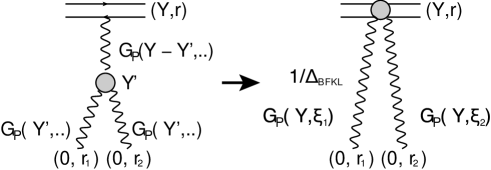
Figure 2: The graphic form of Eq. (III.3.2). The wavy lines describe the BFKL Pomerons. The blob corresponds to triple Pomeron vertex. Factor $1/\Delta_{\mbox{\tiny BFKL}}$ stems from integration over $Y^{\prime}$ the triple Pomeron diagram.

III.3.3 $\bar{\rho}_{3}\left(Y,r,r_{1},b_{1},r_{2},b_{2},r_{3},b_{2}\right)$

From Eq. (26) we have the following equation for $\bar{\rho}_{3}\left(Y,k_{T},r_{1},b_{1},r_{2},b_{2},r_{3},b_{2}\right)$ :

$$\int d^{2}\,r^{\prime}K\left(\bm{r}^{\prime},\bm{r}-\bm{r^{\prime}}|\bm{r}\right)\Bigg{\{}\Bigg{(}\,\bar{\rho}_{3}(Y,\bm{r}^{\prime},\bm{b}-\frac{1}{2}(\bm{r}-\bm{r}^{\prime});\bm{r}_{1},b_{1},\bm{r}_{2},b_{2},\bm{r}_{3},b_{3})\,+\,\,\bar{\rho}_{3}(Y,\bm{r}-\bm{r}^{\prime},\bm{b}-\frac{1}{2}\bm{r}^{\prime};\bm{r}_{1},b_{1},\bm{r}_{2},b_{2},\bm{r}_{3},b_{3})$$

$$- \bar{\rho}_{3}(Y,\bm{r},\bm{b};\bm{r}_{1},b_{1},\bm{r}_{2},b_{2})\Bigg{)}+\bar{\rho}_{1}(Y,\bm{r}^{\prime},\bm{b};\bm{r}_{1},\bm{b}_{1})\,\bar{\rho}_{2}(Y,\bm{r}-\bm{r}^{\prime},\bm{b};\bm{r}_{2},\bm{b}_{2},\bm{r}_{3},b_{3})$$

$$\,+ \,\bar{\rho}_{2}(Y,\bm{r}^{\prime},\bm{b};\bm{r}_{1},\bm{b}_{1},\bm{r}_{3},b_{3})\,\bar{\rho}_{1}(Y,\bm{r}-\bm{r}^{\prime},\bm{b};\bm{r}_{2},\bm{b}_{2})\Bigg{\}}\,\,=\,\,\int\,\frac{d^{2}\,r^{\prime}}{2\,\pi}\,K\left(\bm{r}^{\prime},\bm{r}_{1}-\bm{r^{\prime}}|\bm{r}_{1}\right)\,$$

$$\times \Big{\{}\bar{\rho}_{3}\left(Y,\bm{k}_{T};\bm{r}^{\prime},b_{1},\bm{r}_{2},b_{2},\bm{r}_{3},b_{3}\right)\,\,+\,\,\bar{\rho}_{3}\left(Y,\bm{k}_{T};\bm{r}_{1}-\bm{r}^{\prime},b_{1},\bm{r}_{2},b_{2},\bm{r}_{3},b_{3}\right)\,-\,\bar{\rho}_{3}\left(Y,\bm{k}_{T},\bm{r}_{1},b_{1},\bm{r}_{2},b_{2},\bm{r}_{3},b_{3}\right)\Big{\}}$$

$$+ \int\,\frac{d^{2}\,r^{\prime}}{2\,\pi}\,K\left(\bm{r}^{\prime},\bm{r}_{2}-\bm{r^{\prime}}|\bm{r}_{2}\right)\,$$

$$\times \Big{\{}\bar{\rho}_{3}\left(Y,\bm{r};\bm{r}_{1},b_{1},\bm{r}^{\prime},b_{2},\bm{r}_{3},b_{3}\right)\,\,+\,\,\bar{\rho}_{3}\left(Y,\bm{r};\bm{r}_{1},b_{1},\bm{r}_{2}-\bm{r}^{\prime},b_{2},\bm{r}_{3},b_{3}\right)\,-\,\bar{\rho}_{2}(Y,\bm{r};\bm{r}_{1},b_{1},\bm{r}_{2},b_{2},\bm{r}_{3},b_{3})\Big{\}}$$

$$+ \,\,\,\int\,\frac{d^{2}\,r^{\prime}}{2\,\pi}\,K\left(\bm{r}^{\prime},\bm{r}_{3}-\bm{r^{\prime}}|\bm{r}_{3}\right)\,$$

$$\times \Big{\{}\bar{\rho}_{3}\left(Y,\bm{r};\bm{r}_{1},b_{1},\bm{r}_{2},b_{2},\bm{r}^{\prime},b_{3}\right)\,\,+\,\,\bar{\rho}_{3}\left(Y,\bm{r};\bm{r}_{1},b_{1},\bm{r}_{2},b_{2},\bm{r}_{3}-\bm{r}^{\prime},b_{3}\right)\,-\,\bar{\rho}_{2}(Y,\bm{r};\bm{r}_{1},b_{1},\bm{r}_{2},b_{2},\bm{r}_{3},b_{3})\Big{\}}$$

$$+ \,\,\,\,\,\Big{\{}\bar{\rho}_{2}(Y,\bm{r};\bm{r}_{1}+\bm{r}_{3},b_{1},\bm{r}_{2},b_{2})\,\,+\,\,\bar{\rho}_{2}(Y,\bm{r};\bm{r}_{1},b_{1},\bm{r}_{2}+\bm{r}_{3},b_{2})\Big{\}}$$

Replacing $\int d^{2}\,r^{\prime}K\left(\bm{r}^{\prime},\bm{r}-\bm{r^{\prime}}|\bm{r}\right)\,\{\dots\}=\Delta_{\mbox{\tiny BFKL}}\bar{\rho}_{3}(Y,\bm{r};\bm{r}_{1},\bm{b}_{1},\bm{r}_{2},\bm{b}_{2},\bm{r}_{3},\bm{b}_{3})$ we obtain that

$$\bar{\rho}_{3}(Y,\bm{r};\bm{r}_{1},\bm{b}_{1},\bm{r}_{2},\bm{b}_{2},\bm{r}_{3},\bm{b}_{3})\,\,=\,\,\frac{1}{2}\Bigg{\{}\frac{\bar{\alpha}_{S}}{\Delta_{\mbox{\tiny BFKL}}}\int d^{2}\,r^{\prime}K\left(\bm{r}^{\prime},\bm{r}-\bm{r^{\prime}}|\bm{r}\right)$$

$$\times \Big{\{}\bar{\rho}_{2}(Y,\bm{r}^{\prime},\bm{b};\bm{r}_{1},\bm{b}_{1},\bm{r}_{3},\bm{b}_{2})\,\,\bar{\rho}_{1}(Y,\bm{r}-\bm{r}^{\prime},\bm{b};\bm{r}_{2},\bm{b}_{2})\,\,+\,\,\bar{\rho}_{1}(Y,\bm{r}^{\prime},\bm{b};\bm{r}_{1},\bm{b}_{1})\,\,\bar{\rho}_{2}(Y,\bm{r}-\bm{r}^{\prime},\bm{b};\bm{r}_{2},\bm{b}_{2},\bm{r}_{3},\bm{b}_{3})\Big{\}}\,\,$$

$$-\,\,\Big{\{}\bar{\rho}_{2}(Y,\bm{r};\bm{r}_{1}+\bm{r}_{3},b_{1},\bm{r}_{2},b_{2})\,\,+\,\,\bar{\rho}_{2}(Y,\bm{r};\bm{r}_{1},b_{1},\bm{r}_{2}+\bm{r}_{3},b_{2})\Big{\}}\Bigg{\}}$$

This equation has a simplified form in the momentum representation (see Eq. (35)):

$$\bar{\rho}_{3}(Y,\bm{k}_{T};\bm{r}_{1},\bm{b}_{1},\bm{r}_{2},\bm{b}_{2},\bm{r}_{3},\bm{b}_{3})\,\,=\,\,\frac{1}{2}\Bigg{(}\frac{\bar{\alpha}_{S}}{\Delta_{\mbox{\tiny BFKL}}}\Bigg{)}\Bigg{\{}\bar{\rho}_{2}(Y,\bm{k}_{T},\bm{b};\bm{r}_{1},\bm{b}_{1},\bm{r}_{3},\bm{b}_{2})\bar{\rho}_{1}(Y,\bm{k}_{T},\bm{b};\bm{r}_{2},\bm{b}_{2})\,\,$$ (44)

$$+\,\,\bar{\rho}_{1}(Y,\bm{k}_{T},\bm{b};\bm{r}_{1},\bm{b}_{1})\,\bar{\rho}_{2}(Y,\bm{k}_{T},\bm{b};\bm{r}_{2},\bm{b}_{2},\bm{r}_{3},\bm{b}_{2})\,\,-\,\,\Big{(}\bar{\rho}_{2}(Y,\bm{k}_{T};\bm{r}_{1}+\bm{r}_{3},b_{1},\bm{r}_{2},b_{2})\,\,+\,\,\bar{\rho}_{2}(Y,\bm{k}_{T};\bm{r}_{1},b_{1},\bm{r}_{2}+\bm{r}_{3},b_{2})\Big{)}\Bigg{\}}$$

For the toy model in which $\bar{\rho}_{n}$ do not depend on the dipole sizes, Eq. (44) leads to $\bar{\rho}_{3}\,\,=\,\,\bar{\rho}_{1}\left(\bar{\rho}_{1}\,-\,1\right)^{2}$, if we assume that $\Delta_{\mbox{\tiny BFKL}}\,=\,\bar{\alpha}_{S}$. One can see that the calculations started to be cumbersome, but for our approach the most important conclusions is that the main contributions, which is proportional to $e^{3\,\Delta_{\mbox{\tiny BFKL}}\,Y}$, has a very simple form:

$$\bar{\rho}_{3}(Y,\bm{k}_{T};\bm{r}_{1},\bm{b}_{1},\bm{r}_{2},\bm{b}_{2},\bm{r}_{3},\bm{b}_{3})\,\,=$$ (45)

$$\,\,\Bigg{(}\frac{\bar{\alpha}_{S}}{\Delta_{\mbox{\tiny BFKL}}}\Bigg{)}^{2}\bar{\rho}_{1}(Y,\bm{k}_{T},\bm{b};\bm{r}_{1},\bm{b}_{1})\,\bar{\rho}_{1}(Y,\bm{k}_{T},\bm{b};\bm{r}_{2},\bm{b}_{2})\,\bar{\rho}_{1}(Y,\bm{r},\bm{b};\bm{r}_{3},\bm{b}_{3})\,\,+\,\,{\cal O}\left(e^{2\,\Delta_{\mbox{\tiny BFKL}}\,Y}\right)\Bigg{\}}$$

$$\,\,\Bigg{(}\frac{\bar{\alpha}_{S}}{\Delta_{\mbox{\tiny BFKL}}}\Bigg{)}^{2}\bar{\rho}^{\rm d.a}_{1}\left(Y;\xi^{\prime}_{1}\right)\,\bar{\rho}^{\rm d.a.}_{1}\left(Y;\xi^{\prime}_{2}\right)\,\bar{\rho}^{\rm d.a.}_{1}\left(Y;\xi^{\prime}_{3}\right)\,\,=\,\,\left(\frac{\bar{\alpha}_{S}}{\Delta_{\mbox{\tiny BFKL}}}\right)^{2}G_{I\!\!P}\left(Y;\xi^{\prime}_{1}\right)\,G_{I\!\!P}\left(Y;\xi^{\prime}_{2}\right)\,G_{I\!\!P}\left(Y;\xi^{\prime}_{3}\right)$$

We see again that at large $Y$ $\bar{\rho}_{3}$ is described by the ‘fan’ diagram of the same type as in Fig. 2, but with three Pomerons, in which two integrations of the positions of two triple Pomeron vertices lead to factor $(1/\Delta_{\mbox{\tiny BFKL}})^{2}$ while $\bar{\alpha}_{S}^{2}$ appears due to the value of the triple Pomeron vertex is equal to $\bar{\alpha}_{S}$ and we have two vertices in these diagrams.

III.3.4 $\bar{\rho}_{n}\left(Y,\bm{r},\{\bm{r}_{i},b_{i}\}\right)$ at high energies

Having solutions for $\bar{\rho}_{2}$ and $\bar{\rho}_{3}$, one can see that the leading term of the solution to Eq. (26) , which behaves as $\exp\left(n\Delta_{\mbox{\tiny BFKL}}\,Y\right)$ at high energies, has the form:

$$\bar{\rho}_{n}(Y,\{\xi^{\prime}_{i}\})\,\,=\,\,\Bigg{(}\frac{\bar{\alpha}_{S}}{\Delta_{\mbox{\tiny BFKL}}}\Bigg{)}^{n-1}\underbrace{\prod^{n}_{i=1}\bar{\rho}^{\rm d.a.}_{1}\left(Y;\xi^{\prime}_{i}\right)}_{\sim\exp\left(n\Delta_{\mbox{\tiny BFKL}}\,Y\right)}$$ (46)

We can check by the direct substitution in Eq. (26) that $\bar{\rho}_{n}$ is equal to

$$\bar{\rho}_{n}(Y,\{\xi_{i}\})\,\,=\,\,\Bigg{(}\frac{\bar{\alpha}_{S}}{\Delta_{\mbox{\tiny BFKL}}}\Bigg{)}^{n-1}\Bigg{\{}\underbrace{\prod^{n}_{i=1}\bar{\rho}^{\rm d.a.}_{1}\left(Y;\xi_{i}\right)}_{\sim\exp\left(n\Delta_{\mbox{\tiny BFKL}}\right)}\,\,-\,\,\frac{1}{n-1}\underbrace{\sum_{i=1}^{n-1}\bar{\rho}^{\rm d.a.}_{n-1}(\{\xi_{j},\xi_{i,n}\})}_{\sim\exp\left((n-1)\Delta_{\mbox{\tiny BFKL}}\right)}\Bigg{\}}$$ (47)

Accuracy of this solution is of the order of $n\,\left(\xi^{2}_{i}/(4\,D\,Y)\right)^{2}$ and we will show below that the typical values of $n$ does not increase with $Y$.

IV Scattering amplitude

IV.1 The BFKL Pomeron exchange

From Eq. (27) the contribution of the single BFKL Pomeron exchange to the scattering amplitude is equal to the following expressionMUDI :

$$A^{\mbox{\tiny BFKL}}\left(Y,\bm{k}_{T},\bm{k}_{T}^{\prime};\bm{b}\right)\,\,=\,\,\int\frac{d^{2}\,r_{1}}{r^{4}_{2}}\frac{d^{2}\,r^{\prime}_{1}}{r^{\prime 4}_{1}}\,d^{2}b^{\prime}_{1}\,\bar{\rho}\left(Y-Y_{0},\bm{k}_{T};\bm{r}_{1},\bm{b}-\bm{b}^{\prime}_{1}\right)\,\,\sigma^{\rm BA}\left(\bm{r}_{1},\bm{r}^{\prime}_{1}\right)\,\,\bar{\rho}\left(Y_{0},\bm{k}_{T}^{\prime};\bm{r}^{\prime}_{1},\bm{b}^{\prime}_{1}\right)$$ (48)

where $\bm{k}_{T}^{\prime}$ appears as momentum variable corresponding the $R$-dependece of the scattering amplitude.

Eq. (48) has been estimated (see Refs.MUDI ; Salam ) , however, for completeness of presentation, we briefly outline here the main points of these estimates. Plugging Eq. (32) and Eq. (28) into Eq. (48) we can first integrate over $r_{1}$ and $r^{\prime}_{1}$, obtaining the contribution $\propto\,\,l^{2+2i\nu\,+\,2\,i\,\nu^{\prime}}$, with $\gamma_{r}=\frac{1}{2}+i\,\nu$ and $\gamma^{\prime}_{r^{\prime}}=\frac{1}{2}+i\nu^{\prime}$. Integration over $l$ leads to the pole $1/(\nu\,+\nu^{\prime})$, which contribution leads to the independence of the amplitude with the value of $Y_{0}$. The integral over $d^{2}b^{\prime}_{1}$ has the form

$$\int d^{2}b^{\prime}_{1}\frac{1}{\left(\left(\bm{b}\,-\,\bm{b}^{\prime}_{1}\right)^{2}\,b^{\prime 2}_{1}\right)^{1+i\,\nu}}\,\,=\,\,\frac{2}{i\nu}\frac{1}{b^{2(1+i\nu)}}$$ (49)

In Eq. (49) the main contributions stem from two kinematic regions: $b^{\prime}_{1}\ll b$ and $|\bm{b}-\bm{b}^{\prime}_{1}|\,\ll\,b$. Finally we obtain the result of Ref.MUDI :

$$A^{\mbox{\tiny BFKL}}\left(Y,\bm{k}_{T},\bm{k}_{T}^{\prime};\bm{b}\right)\,\,=$$ (50)

$$\frac{8\bar{\alpha}_{S}^{2}\,\pi}{\left(D\,Y\right)^{3/2}}\,\frac{4}{k_{T}\,k^{\prime}_{T}\,b^{2}}\,\ln\left(\frac{k_{T}\,k^{\prime}_{T}\,b^{2}}{4}\right)\,\exp\left(\Delta_{\mbox{\tiny{BFKL}}}\,Y-\frac{\ln^{2}\left(\frac{16}{b^{4}\,k^{2}_{T}\,k^{\prime 2}_{T}}\right)}{4\,D\,Y}\right)\,\,=\,\,\frac{8\,\pi\bar{\alpha}_{S}^{2}}{\left(D\,Y\right)^{3/2}}\,\xi\,e^{-\xi}\,\exp\left(\Delta_{\mbox{\tiny{BFKL}}}\,Y-\frac{\xi^{2}}{4\,D\,Y}\right)$$

where $\xi=\ln\left(\frac{k_{T}\,k^{\prime}_{T}b^{2}}{4}\right)$.

IV.2 Scattering amplitude from the main formula in the momentum representation

Plugging Eq. (50) into our master equation (see Eq. (27)) one can see that the scattering amplitude takes the following form:

$$A\left(Y,\bm{k}_{T},\bm{k}_{T}^{\prime};\bm{b}\right)\,=\,\sum^{\infty}_{n=1}\,\left(-1\right)^{n+1}\,n!\,\Bigg{(}\frac{{\bar{\alpha}_{S}^{2}}}{\Delta^{2}_{\mbox{\tiny BFKL}}}\Bigg{)}^{n-1}\left(A^{\mbox{\tiny BFKL}}\left(Y,k_{T},k^{\prime}_{T};\bm{b}\right)\right)^{n}$$

$$\,\,=\,\,\Bigg{(}\frac{\Delta^{2}_{\mbox{\tiny BFKL}}}{\bar{\alpha}_{S}^{2}}\Bigg{)}\Bigg{\{}1\,\,-\,\,e^{\frac{1}{\kappa}}\,\Gamma\left(0,\frac{1}{\kappa}\right)/\kappa\Bigg{\}}\,\,\rightarrow\,\,\left\{\begin{array}[]{l}\,\,\,\Big{(}\frac{\Delta^{2}_{\mbox{\tiny BFKL}}}{\bar{\alpha}_{S}^{2}}\Big{)}\,\kappa=A^{\mbox{\tiny BFKL}}\left(Y,r,R;\bm{b}\right)\,\,\,\,\,\,\,\,\,\mbox{for}\,\,\,\kappa\,\ll\,1;\\ \\ \,\,\Big{(}\frac{\Delta^{2}_{\mbox{\tiny BFKL}}}{\bar{\alpha}_{S}^{2}}\Big{)}\Bigg{(}1\,+\frac{-\ln\kappa\,\,+C_{E}}{\kappa}\Bigg{)}\,\,\,\mbox{for}\,\,\,\kappa\,\gg\,1;\\ \end{array}\right.$$ (54)

where $\kappa=\Big{(}\frac{\bar{\alpha}_{S}^{2}}{\Delta^{2}_{\mbox{\tiny BFKL}}}\Big{)}A^{\mbox{\tiny BFKL}}\left(Y,\bm{k}_{T},\bm{k}_{T}^{\prime};\bm{b}\right)$. One can see that at low energies (small values of $Y$) the scattering amplitude reproduces the exchange of one BFKL Pomeron. At high energies ( at $Y\,\,\gg\,\,1$) the amplitude approaches the constant value $\Big{(}\frac{\Delta_{\mbox{\tiny BFKL}}}{\bar{\alpha}_{S}}\Big{)}$. Since this amplitude is in the momentum representation, the unitarity limit for it is $\frac{1}{2}\ln k^{2}_{T}\frac{1}{2}\ln k^{\prime 2}_{T}$, but not the unity.

The scattering amplitude of Eq. (IV.2) does not generate a correct behaviour of the cross section, which increases as a power of the energy, resulting from the power-like bahaviour of the scatterring amplitude at large impact parameters. From Eq. (IV.2) one can see that the corrections at large values of $Y$ show the increase with the growth of $b$, demonstrating that in the scattering amplitude we have even more severe problems with the Froissart theoremFROI than for the BK evolutionKW1 ; KW2 ; KW3 ; FIIM .

In all our estimates we assume that $\sum^{n}_{1}\frac{\xi^{\prime}_{i}}{2\,D,Y}\,\,\ll\,\,1$. Therefore, we need to estimate the typical values of $n$ in this sum. From Eq. (IV.2) we can find the average value of $n$:

$$\bar{n}\,=\frac{d\,\ln A\left(Y,r,R;\bm{b}\right)}{d\ln A^{\rm BFKL}}=\,\,\Bigg{(}\frac{\mu e^{1/\kappa}\Gamma\left(0,\frac{1}{\kappa}\right)}{\kappa^{2}}-\frac{\mu}{\kappa}+\frac{\mu e^{1/\kappa}\Gamma\left(0,\frac{1}{\kappa}\right)}{\kappa}\Bigg{)}\Bigg{/}\Bigg{(}1-\frac{\mu e^{1/\kappa}\Gamma\left(0,\frac{1}{\kappa}\right)}{\kappa}\Bigg{)}$$ (55)

where $\kappa=\Big{(}\frac{\bar{\alpha}_{S}^{2}}{\Delta^{2}_{\mbox{\tiny BFKL}}}\Big{)}A^{\mbox{\tiny BFKL}}\left(Y,r,R;\bm{b}\right)$ and $\mu=\Delta^{2}_{\mbox{\tiny BFKL}}/{\bar{\alpha}_{S}^{2}}$. One can see that $\bar{n}$ decreases at large values of $Y$. Therefore, our assumption $\sum^{n}_{1}\frac{\xi^{\prime}_{i}}{2\,D,Y}\,\,\ll\,\,1$ looks plausible.

One can also see that at fixed $b$, the scattering amplitude approaches the constant value of $\Delta_{\mbox{\tiny BFKL}}/{\bar{\alpha}_{S}}$ as follows

$$A\left(Y,\bm{k}_{T},\bm{k}_{T}^{\prime};\bm{b}\right)\,\,=\,\,1\,\,-\,\,{\rm Const}\ln\left(A^{\mbox{\tiny BFKL}}\left(Y,r,R;\bm{b}\right)\right)/A^{\mbox{\tiny BFKL}}\left(Y,\bm{k}_{T},\bm{k}_{T}^{\prime};\bm{b}\right)\,\,=\,\,1\,-\,{\cal C}\left(\xi^{\prime},Y\right)\left(e^{\xi^{\prime}}\,Q^{2}_{s}(Y)\right)^{-\bar{\gamma}}$$ (56)

where the saturation momentum $Q^{2}_{s}(Y)\,=\,\exp\left(2\,D\,Y\left(1+\frac{\Delta_{\mbox{\tiny BFKL}}}{D}\right)\right)$,$\bar{\gamma}\,=\,\frac{1}{2}+\frac{\Delta_{\mbox{\tiny BFKL}}}{D}$ and function ${\cal C}$ is a smooth function of $\xi$ and $Y$.

It is instructive to note that at first sight such approach is in contradiction both with BK non-linear evolution equationLETU and with estimates for the scattering dipole-dipole amplitude in Ref. IAMU1 . However, we will show in the next section that it is not the case, considering the solution to BK non-linear equation in the diffusion approximation for the BFKL kernel.

IV.3 Solution to BK equation with the diffusion kernel at high energies

The surprising result is that the amplitude in the momentum representation turns out to be constant at high energies and it does not show the geometric scaling behaviour. In this section we show that both these features are the artifact of the simplified BFKL kernel that we have used. As have been discussed we used the diffusion approximation of Eq. (31) (at $\gamma\to\frac{1}{2}$) for the BFKL kernel. The BK equation in the momentum representation ($k_{T}$) takes the following form:

$$\frac{\partial\widetilde{N}\left(k_{\perp},b;Y\right)}{\partial Y}\,\,=\,\,\bar{\alpha}_{S}\Bigg{\{}\chi\left(-\,\frac{\partial}{\partial\tilde{\xi}}\right)\widetilde{N}\left(k_{\perp},b;Y\right)\,\,\,-\,\,\widetilde{N}^{2}\left(k_{\perp},b;Y\right)\Bigg{\}}$$ (57)

with $\tilde{\xi}=\ln k^{2}_{T}$ and

$$\bar{\alpha}_{S}\,\chi\left(-\,\frac{\partial}{\partial\tilde{\xi}}\right)\,\,=\,\,\Delta_{\mbox{\tiny BFKL}}\,\,+\,\,D\,\frac{\partial^{2}}{\partial\tilde{\xi}^{2}}$$ (58)

(see Eq. (31) at $\gamma\to\frac{1}{2}$).

The asymptotic solution to Eq. (57) has a simple form: $\widetilde{N}^{\rm asymp}\left(k_{\perp}\right)=\frac{\Delta_{\mbox{\tiny BFKL}}}{\bar{\alpha}_{S}}$. Plugging in Eq. (57) $\widetilde{N}\left(k_{\perp},b;Y\right)\,\,=\,\,\widetilde{N}^{\rm asymp}\left(k_{\perp}\right)\,\,-\,\,\Delta\widetilde{N}\left(k_{\perp},b;Y\right)$ and considering $\Delta\widetilde{N}\left(k_{\perp},b;Y\right)\,\,\ll\,\,1$ we obtain the following linear equation for $\Delta\widetilde{N}\left(k_{\perp},b;Y\right)$:

$$\frac{\partial\Delta\widetilde{N}\left(k_{\perp},b;Y\right)}{\partial Y}\,\,=\,\,-\Delta_{\mbox{\tiny BFKL}}\Delta\widetilde{N}\left(k_{\perp},b;Y\right)\,\,+\,\,D\,\frac{\partial^{2}}{\partial\tilde{\xi}^{2}}\,\Delta\widetilde{N}\left(k_{\perp},b;Y\right)$$ (59)

Eq. (59) has the same form as the linear BFKL equation but with the negative intercept. Hence, the solution to Eq. (59) can be obtain from Eq. (36) :

$$\Delta\widetilde{N}\left(k_{\perp},b;Y\right)\,\,=\,\,\frac{2}{\left(D\,Y\right)^{3/2}}\,\xi^{\prime}\,e^{-\Delta_{\mbox{\tiny{BFKL}}}\,Y-\frac{\xi^{\prime 2}}{4\,D\,Y}}\,e^{\frac{1}{2}\xi^{\prime}}$$ (60)

Therefore, one can see that (i) the solution at high energies does not show the geometric scaling behaviour which was predicted in Ref.LETU ; and (ii) at large $Y$ it decreases as $\exp\left(-{\rm Const}Y\right)$ instead of $\exp\left(-{\rm Const}Y^{2}\right)$LETU . Note, that we use the same procedure to Eq. (57) as was developed in Ref.LETU to the general kernel of the BFKL equation. On the other hand, applying the approach of Ref.IAMU1 to the scattering amplitude taking into account Eq. (60) we obtain Eq. (IV.2) for $\kappa\gg 1$.

Concluding, we state that the scattering amplitude of Eq. (IV.2) gives more microscopic insight in the structure of the scattering amplitude and reproduces both approaches of Refs.IAMU ; LETU . It worth mentioning that Eq. (57), being F-KPP equationsF ; KPP , shows the geometrical scaling behaviour in pre-asymptotic region in the vicinity of the saturation scale. Eq. (60) also indicates that our assumption: $\xi/Y\,\,\ll\,1$ is not substantial for the main features of the amplitude behaviour.

IV.4 Dipole-dipole scattering amplitude at high energies

The dipole-dipole scattering amplitude takes the following form:

$$A\left(Y,r,R;\bm{b}\right)\,\,=\,\,r^{2}\,R^{2}\,\int k_{T}\,dk_{T}J_{0}\left(k_{T}\,r\right)\,\int k^{\prime}_{T}\,dk^{\prime}_{T}J_{0}\left(k^{\prime}_{T}\,R\right)\,\,A\left(Y,\bm{k}_{T},\bm{k}_{T}^{\prime};\bm{b}\right)$$ (61)

We use the Mellin transform for $J_{0}(k_{T}\,r)$ (see formula 6.8.1 of Ref.BATEMAN ) :

$$J_{0}(k_{T}\,r)\,\,=\,\,\int^{\epsilon+i\infty}_{\epsilon-i\infty}\frac{d\gamma}{2\,\pi\,i}(k_{T}\,r)^{-\gamma}\frac{2^{\gamma-1}\Gamma\left(\frac{1}{2}\gamma\right)}{\Gamma\left(1-\frac{1}{2}\gamma\right)}$$ (62)

Note, that in Eq. (62) we take $\frac{3}{2}>\epsilon>1$.

Introducing a new variable $k_{T}\,k^{\prime}_{t}\,=\zeta$ we can rewrite Eq. (61) in the form:

$$A\left(Y,r,R;\bm{b}\right)\,\,=$$ (63)

$$\,\,r^{2}\,R^{2}\,\int\zeta d\zeta\frac{dk_{T}}{k_{T}}\,\int^{\epsilon+i\infty}_{\epsilon-i\infty}\frac{d\gamma}{2\,\pi\,i}(k_{T}\,r)^{-\gamma}\frac{2^{\gamma-1}\Gamma\left(\frac{1}{2}\gamma\right)}{\Gamma\left(1-\frac{1}{2}\gamma\right)}\int^{\epsilon+i\infty}_{\epsilon-i\infty}\frac{d\gamma}{2\,\pi\,i}\left(\frac{\zeta}{k_{T}}\,R\right)^{-\gamma^{\prime}}\frac{2^{\gamma^{\prime}-1}\Gamma\left(\frac{1}{2}\gamma^{\prime}\right)}{\Gamma\left(1-\frac{1}{2}\gamma^{\prime}\right)}\,\,A\left(Y,\bm{k}_{T},\bm{k}_{T}^{\prime};\bm{b}\right)$$

Noting that $A\left(Y,\bm{k}_{T},\bm{k}_{T}^{\prime};\bm{b}\right)$ depends only on $\zeta$, we can integrate Eq. (63) over $k_{T}$ and $\gamma^{\prime}$ , which results in:

$$A\left(Y,r,R;\bm{b}\right)\,\,=\,\,r^{2}\,R^{2}\,\int\zeta d\zeta\,\int^{\epsilon+i\infty}_{\epsilon-i\infty}\frac{d\gamma}{2\,\pi\,i}\left(\zeta\,R\,r\right)^{-\gamma}\frac{4^{\gamma-1}\Gamma^{2}\left(\frac{1}{2}\gamma\right)}{\Gamma^{2}\left(1-\frac{1}{2}\gamma\right)}\,\,A\left(Y,\bm{k}_{T},\bm{k}_{T}^{\prime};\bm{b}\right)$$ (64)

To take integral over $\zeta$ we simplify the expression for $A^{\mbox{\tiny BFKL}}\left(Y,\bm{k}_{T},\bm{k}_{T}^{\prime};\bm{b}\right)$ of Eq. (50) considering $\gamma_{SP}=\frac{1}{2}$ and reducing it to the following expression:

$$A^{\mbox{\tiny BFKL}}\left(Y,\bm{k}_{T},\bm{k}_{T}^{\prime};\bm{b}\right)\,\, = \,\,\frac{8\,\pi}{\left(D\,Y\right)^{3/2}}\,\frac{4}{k_{T}\,k^{\prime}_{T}\,b^{2}}\,\ln\left(\frac{k_{T}\,k^{\prime}_{T}\,b^{2}}{4}\right)\,\exp\left(\Delta_{\mbox{\tiny{BFKL}}}\,Y-\frac{\ln^{2}\left(\frac{16}{b^{4}\,k^{2}_{T}\,k^{\prime 2}_{T}}\right)}{4\,D\,Y}\right)$$ (65)

$$\,\,=\,\, \frac{1}{k_{T}\,k^{\prime}_{T}}N\left(k_{T}\to 2/r;k^{\prime}_{T}\to 2/R\right)\,\,=\,\,\frac{N}{\zeta}$$

where we use Eq. (36). The new variable $\zeta=k_{T}\,k^{\prime}_{T}$.

Using the integral representation for the incomplete gamma function (see formula 8.353(3) in Ref.RY ) and Eq. (65) we obtain:

$$A\left(Y,r,R;\bm{b}\right)\,\, = \,\,\mu\,r^{2}\,R^{2}\,\int\zeta d\zeta\,\int^{\epsilon+i\infty}_{\epsilon-i\infty}\frac{d\gamma}{2\,\pi\,i}(\zeta\,R\,r)^{-\gamma}\frac{4^{\gamma-1}\Gamma^{2}\left(\frac{1}{2}\gamma\right)}{\Gamma^{2}\left(1-\frac{1}{2}\gamma\right)}\,\int^{\infty}_{0}d\tau e^{-\tau}\frac{\frac{\tau\,N}{\mu\,\zeta}}{1+\frac{\tau\,N}{\mu\,\zeta}}$$ (66)

$$= \mu\,r^{2}\,R^{2}\,\int\zeta d\zeta\,\int^{\epsilon+i\infty}_{\epsilon-i\infty}\frac{d\gamma}{2\,\pi\,i}(R\,r)^{-\gamma}\frac{4^{\gamma-1}\Gamma^{2}\left(\frac{1}{2}\gamma\right)}{\Gamma^{2}\left(1-\frac{1}{2}\gamma\right)}\,\int^{\infty}_{0}d\tau e^{-\tau}\Bigg{\{}-\frac{\pi}{\sin\left(\pi\,\gamma\right)}\left(\tau\,N/\mu\right)^{(2-\gamma)}\Bigg{\}}$$

$$= \mu\int^{\epsilon+i\infty}_{\epsilon-i\infty}\frac{d\gamma}{2\,\pi\,i}\frac{4^{\gamma-1}\Gamma^{2}\left(\frac{1}{2}\gamma\right)}{\Gamma^{2}\left(1-\frac{1}{2}\gamma\right)}\Bigg{(}-\frac{\pi}{\sin\left(\pi\,\gamma\right)}\Bigg{)}\left(r\,R\,N/\mu\right)^{2-\gamma}$$

Closing contour of integration over $\gamma$ on negative $\gamma$ we obtain the scattering amplitude as sum of $\left(r\,R\,N=A^{\mbox{\tiny BFKL}}\left(Y,\xi_{r}\right)\right)^{n}$ , where $\xi_{r}=\ln\left(\frac{b^{2}}{r\,R}\right)$. If we close the contour on the singularities for positive $\gamma>1$, we have the asymptotic series , which determines the behaviour of the scattering amplitude at high energies (at large values of $Y$). One can see that the integrant has no singularities at $\gamma=2$ and the first pole appears at $\gamma=3$, which leads to

$$A\left(Y,r,R;\bm{b}\right)\,\,=\,\,\mu^{2}\frac{\ln\left(A^{\mbox{\tiny BFKL}}\left(Y,\xi_{r}\right)/\mu\right)}{A^{\mbox{\tiny BFKL}}\left(Y,\xi_{r}\right)}$$ (67)

where $\mu\,=\,\Delta_{\mbox{\tiny BFKL}}/{\bar{\alpha}_{S}}$.

Therefore, we found that the scattering amplitude decreases at large values of $Y$ (at high energies).

V Conclusions

In this paper we have three results. First, we derived the recurrence relations for dipole densities ($\rho_{n}$) in QCD for the BFKL parton cascade. These relations allow us to find the dipole densities from the solution to the BFKL equation for $\rho_{1}$. Note, that Eq. (III.1) for the energy evolution of the parton densities is also new. Second, using the diffusion approximation for the BFKL kernel, we resolve these recurrence relations and found the leading terms in $\rho_{n}\propto e^{n\,\Delta_{\mbox{\tiny BFKL}}\,Y}$. It is worth mentioning that these relations are suited for the numerical estimate of the dipole densities opening a new way for the numerical simulation of the scattering amplitudes using Eq. (27).

Third, for the first time we sum analytically the large Pomeron loops in QCD using these solutions. As a result of this summation we obtain the dipole-dipole scattering amplitude. Surprisingly, it turns out that this amplitude decreases at large values of $Y$. We believe that such a behaviour of the scattering amplitude follows from the simplified kernel of the BFKL equation in the diffusion approximation, as has been demonstrated in section IV-C. The physics origin of such behaviour is that the diffusion BFKL kernel does not lead to the saturation both in BK equation and in dipole-dipole amplitude. In other words, the first attempt to sum analytically BFKL Pomeron loops in QCD leads to the scattering amplitude that satisfies both $t$ and $s$ channel unitarity without saturation. Hence, the sum of Pomerom loops gives the typical contribution to S-matrix at high energies which turns out to be larger than the rare fluctuations discussed in RefIAMU1 and which will lead to the main contribution to the scattering amplitude for more realistic approximation for the BFKL kernel. The fact that the diffusion approximation to the BFKL kernel is so deficient, turns out to be a great surprise to us, especially because this approximation, which leads to F-KPP equation, has been widely used to describe the deep inelastic scattering (see Ref.KOLEB for review). On the other hand, such a result is not new for the Pomeron calculus (see Ref.BRAUN1 and reference therein). It should be emphasized that shortcomings of the diffusion approximation force us to look at numerical estimates of Refs.MUSA ; Salam with a grain of salt, since the diffusion approximation was used in these papers. We have to believe that these estimates have been made in the pre-asymptotic region where the diffusion approximation generates the geometric scaling behaviour of the scattering amplitude.

Certainly, summing the Pomeron loops for more realistic approximation for the BFKL kernel, that leads to the saturation, will be our first problem to solve in the future. We wish also to note that even in present form the sum of Pomeron loops can be useful in discussion of the multiplicity distribution of the produced gluons.

We believe that our reader can take the following results from this paper. First, it is the new evolution equation for dipole densities (see Eq. (III.1) and the recurrence relation between tthem (see Eq. (26)). They are derived for the general BFKL kernel. The recurrence relations are well suited for the numerical estimates of the scattering amplitudes. Second, it is the solution of Eq. (47), which have been found for the BFKL kernel in diffusion approximation. However, one can use these solutions only in the vicinity of the saturation scale, where they reproduce the geometric scaling behaviourF ; KPP . The third is the unexpected result that the diffusion approximation cannot describe the high energy asymptotic behaviour both for BK equation and for dipole-dipole scattering. The failure of the diffusion approximation is surprising and instructive since most of experts bear in mind the diffusion approximation discussing the BFKL Pomeron contribution.

Acknowledgements

We thank our colleagues at Tel Aviv university and UTFSM for encouraging discussions. Special thanks go A. Kovner and M. Lublinsky for stimulating and encouraging discussions on the subject of this paper. This research was supported by ANID PIA/APOYO AFB180002 (Chile), Fondecyt grant #1180118 (Chile) and the Tel Aviv university encouragement grant #5731.

References

- (1) Yuri V. Kovchegov and Eugene Levin, “ Quantum Chromodynamics at High Energies", Cambridge Monographs on Particle Physics, Nuclear Physics and Cosmology, Cambridge University Press, 2012 .
- (2) V. S. Fadin, E. A. Kuraev and L. N. Lipatov, Phys. Lett. B60, 50 (1975); E. A. Kuraev, L. N. Lipatov and V. S. Fadin, Sov. Phys. JETP 45, 199 (1977), [Zh. Eksp. Teor. Fiz.72,377(1977)]; I. I. Balitsky and L. N. Lipatov, Sov. J. Nucl. Phys. 28, 822 (1978), [Yad. Fiz.28,1597(1978)].
- (3) L. N. Lipatov, Sov. Phys. JETP 63, 904 (1986) [Zh. Eksp. Teor. Fiz. 90, 1536 (1986)].
- (4) L. N. Lipatov, Phys. Rept. 286 (1997) 131.
-
(5)
L. N. Lipatov,
Nucl. Phys. B 365, 614 (1991),
Nucl. Phys. B 452, 369 (1995),
R. Kirschner, L. N. Lipatov and L. Szymanowski, Nucl. Phys. B 425, 579 (1994), Phys. Rev. D 51, 838 (1995). - (6) L. V. Gribov, E. M. Levin and M. G. Ryskin, Phys. Rept. 100, 1 (1983).
- (7) E. M. Levin and M. G. Ryskin, Phys. Rept. 189, 267 (1990).
- (8) A. H. Mueller and J. Qiu, Nucl. Phys. B268 (1986) 427.
-
(9)
A. H. Mueller,
Nucl. Phys. B 415 (1994) 373;
Nucl. Phys. B 437 (1995) 107;
A. H. Mueller and B. Patel, Nucl. Phys. B 425, 471, 1994. - (10) A. H. Mueller and G. P. Salam, Nucl. Phys. B 475, 293 (1996), [hep-ph/9605302].
- (11) G. P. Salam, Nucl. Phys. B 461, 512 (1996); [hep-ph/9509353].
- (12) H. Navelet and R. B. Peschanski, Nucl. Phys. B 507 (1997), 353-366 [arXiv:hep-ph/9703238 [hep-ph]].
- (13) J. Bartels, Z. Phys. C 60 (1993), 471-488 ; J. Bartels and M. Wusthoff, Z. Phys. C 66 (1995), 157-1801; J. Bartels and C. Ewerz, JHEP 09 (1999), 026 [arXiv:hep-ph/9908454 [hep-ph]]; C. Ewerz, JHEP 0104 (2001) 031.
-
(14)
J. Bartels,
Nucl. Phys. B175, 365 (1980);
J. Kwiecinski and M. Praszalowicz, Phys. Lett. B94, 413 (1980). - (15) L. McLerran and R. Venugopalan, Phys. Rev. D49 (1994) 2233, Phys. Rev. D49 (1994), 3352; D50 (1994) 2225; D59 (1999) 09400.
- (16) Y. V. Kovchegov and E. Levin, Nucl. Phys. B 577 (2000) 221.
-
(17)
M. A. Braun,
Eur. Phys. J. C16 (2000) 337;
M. A. Braun and G. P. Vacca, Eur. Phys. J. C6 (1999) 147;
J. Bartels, M. Braun and G. P. Vacca, Eur. Phys. J. C 40, 419 (2005).
J. Bartels, L. N. Lipatov and G. P. Vacca, Nucl. Phys. B 706, 391 (2005). - (18) M. A. Braun, Phys. Lett. B 483, 115 (2000), Eur. Phys. J. C 33, 113 (2004); Phys. Lett. B 632, 297 (2006).
- (19) I. Balitsky, Phys. Rev. D60, 014020 (1999); Y. V. Kovchegov, Phys. Rev. D60, 034008 (1999).
- (20) A. Kovner and M. Lublinsky, JHEP 02 (2007), 058 [arXiv:hep-ph/0512316 [hep-ph]].
- (21) J. Jalilian-Marian, A. Kovner, A. Leonidov, and H. Weigert, , Nucl. Phys. B504 (1997) 415–431, [ arXiv:hep-ph/9701284].
- (22) J. Jalilian-Marian, A. Kovner, A. Leonidov, and H. Weigert, , Phys.Rev. D59 (1998) 014014, [arXiv:hep-ph/9706377 [hep-ph]].
- (23) A. Kovner, J. G. Milhano, and H. Weigert, , Phys. Rev. D62 (2000) 114005, [ arXiv:hep-ph/0004014].
- (24) E. Iancu, A. Leonidov, and L. D. McLerran, ,Nucl. Phys. A692 (2001) 583–645, [ arXiv:hep-ph/0011241].
- (25) E. Iancu, A. Leonidov, and L. D. McLerran, , Phys. Lett. B510 (2001) 133–144, [ arXiv:hep-ph/0102009].
- (26) E. Ferreiro, E. Iancu, A. Leonidov, and L. McLerran, , Nucl. Phys. A703 (2002) 489–538, [ arXiv:hep-ph/0109115].
- (27) H. Weigert, Nucl. Phys. A 703 (2002), 823-860 [arXiv:hep-ph/0004044 [hep-ph]].
- (28) A. Kovner and J. G. Milhano, Phys. Rev. D 61 (2000), 014012 [arXiv:hep-ph/9904420 [hep-ph]].
- (29) T. Altinoluk, A. Kovner, E. Levin and M. Lublinsky, JHEP 04 (2014), 075 [arXiv:1401.7431 [hep-ph]].
- (30) A. Kovner and M. Lublinsky, Phys. Rev. D 71 (2005), 085004 [arXiv:hep-ph/0501198 [hep-ph]].
- (31) A. Kovner and M. Lublinsky, Phys. Rev. Lett. 94, 181603 (2005), [hep-ph/0502119].
- (32) I. Balitsky, Phys. Rev. D 72, 074027 (2005), arXiv:hep-ph/0507237.
- (33) Y. Hatta, E. Iancu, L. McLerran, A. Stasto and D. N. Triantafyllopoulos, Nucl. Phys. A 764, 423 (2006).,arXiv:hep-ph/0504182.
- (34) A. Kovner, M. Lublinsky and U. Wiedemann, JHEP 06 (2007), 075 [arXiv:0705.1713 [hep-ph]]; T. Altinoluk, A. Kovner, M. Lublinsky and J. Peressutti, JHEP 0903, 109 (2009), [arXiv:0901.2559 [hep-ph]].
- (35) A. Kovner, E. Levin, M. Li and M. Lublinsky, JHEP 09 (2020), 199 [arXiv:2006.15126 [hep-ph]].
- (36) A. Kovner, E. Levin, M. Li and M. Lublinsky, JHEP 10 (2020), 185 [arXiv:2007.12132 [hep-ph]].
- (37) D. Amati, L. Caneschi and R. Jengo, Nucl. Phys. B 101 (1975) 397.
- (38) V. Alessandrini, D. Amati and R. Jengo, Nucl. Phys. B 108 (1976) 425.
- (39) R. Jengo, Nucl. Phys. B 108 (1976) 447.
- (40) D. Amati, M. Le Bellac, G. Marchesini and M. Ciafaloni, Nucl. Phys. B 112 (1976) 107.
- (41) M. Ciafaloni, M. Le Bellac and G. C. Rossi, Nucl. Phys. B 130 (1977) 388.
- (42) M. Ciafaloni, Nucl. Phys. B 146 (1978) 427.
- (43) J.-P. Blaizot, E. Iancu and D. N. Triantafyllopoulos, Nucl. Phys. A 784 (2007) 227.
- (44) P. Rembiesa and A. M. Stasto, Nucl. Phys. B 725 (2005) 251.
- (45) A. Kovner and M. Lublinsky, Nucl. Phys. A 767 171 (2006).
- (46) A. I. Shoshi and B. W. Xiao, Phys. Rev. D 73 (2006) 094014.
- (47) M. Kozlov and E. Levin, Nucl. Phys. A 779 (2006) 142.
- (48) N. Armesto, S. Bondarenko, J. G. Milhano and P. Quiroga, JHEP 0805 (2008) 103.
- (49) E. Levin and A. Prygarin, Eur. Phys. J. C 53 (2008) 385.
- (50) A. Kovner, E. Levin and M. Lublinsky, JHEP 08 (2016), 031.
- (51) A. Kovner, E. Levin and M. Lublinsky, JHEP 05, 019 (2022) doi:10.1007/JHEP05(2022)019 [arXiv:2201.01551 [hep-ph]].
- (52) E. Iancu and A. Mueller, Nucl. Phys. A 730 (2004), 494-513 [arXiv:hep-ph/0309276 [hep-ph]].
- (53) E. Iancu and A. Mueller, Nucl. Phys. A 730 (2004), 460-493 [arXiv:hep-ph/0308315 [hep-ph]].
- (54) E. Levin and M. Lublinsky, Phys. Lett. B 607 (2005) 131; Nucl. Phys. A 763 (2005) 172.
- (55) Y. V. Kovchegov, Phys. Rev. D 72 (2005), 094009, [arXiv:hep-ph/0508276 [hep-ph]].
- (56) E. Levin, Nucl. Phys. A 763 (2005), 140-171, [arXiv:hep-ph/0502243 [hep-ph]].
- (57) I. Gradstein and I. Ryzhik, Table of Integrals, Series, and Products, Fifth Edition, Academic Press, London, 1994.
- (58) E. Levin and K. Tuchin, Nucl. Phys. B 573, 833 (2000) [hep-ph/9908317]; Nucl. Phys. A 691, 779 (2001) [hep-ph/0012167]; 693, 787 (2001) [hep-ph/0101275].
- (59) A. D. Le, A. H. Mueller and S. Munier, Phys. Rev. D 104, 034026 (2021), [arXiv:2103.10088 [hep-ph]].
- (60) E. Levin, Phys. Rev. D 104, no.5, 056025 (2021), [arXiv:2106.06967 [hep-ph]].
- (61) M. Froissart, 123 (1961) 1053; A. Martin, “Scattering Theory: Unitarity, Analitysity and Crossing." Lecture Notes in Physics, Springer-Verlag, Berlin-Heidelberg, 1969.
- (62) A. Kovner and U. A. Wiedemann, Phys. Rev. D 66, 051502 (2002) [hep-ph/0112140].
- (63) A. Kovner and U. A. Wiedemann, Phys. Rev. D 66, 034031 (2002) [hep-ph/0204277]; ,̇
- (64) A. Kovner and U. A. Wiedemann, Phys. Lett. B 551, 311 (2003) [hep-ph/0207335].
- (65) E. Ferreiro, E. Iancu, K. Itakura and L. McLerran, Nucl. Phys. A 710, 373 (2002) [hep-ph/0206241].
- (66) Harry Bateman, Tables of integral transforms, McGraw-Hill book company, inc. 1954.
- (67) R.A. Fisher, Ann. Eugen. 7 (1937) 355.
- (68) A. Kolmogorov, I. Petrovskii and N. Piskunov, Bull. Moscow Univ. Math. Mech. 1 (1937) 1.
- (69) A. H. Mueller and D. N. Triantafyllopoulos, Nucl. Phys. B 640 (2002) 331 [hep-ph/0205167]
- (70) E. Iancu, K. Itakura and L. McLerran, Nucl. Phys. A 708 (2002) 327 [hep-ph/0203137].
- (71) M. A. Braun and G. P. Vacca, Eur. Phys. J. C 50, 857-869 (2007), [arXiv:hep-ph/0612162 [hep-ph]].