Identifiability Analysis of Noise Covariances for LTI Stochastic Systems with Unknown Inputs

Abstract

Most existing works on optimal filtering of linear time-invariant (LTI) stochastic systems with arbitrary unknown inputs assume perfect knowledge of the covariances of the noises in the filter design. This is impractical and raises the question of whether and under what conditions one can identify the process and measurement noise covariances (denoted as $Q$ and $R$, respectively) of systems with unknown inputs. This paper considers the identifiability of $Q$/$R$ using the correlation-based measurement difference approach. More specifically, we establish (i) necessary conditions under which $Q$ and $R$ can be uniquely jointly identified; (ii) necessary and sufficient conditions under which $Q$ can be uniquely identified, when $R$ is known; (iii) necessary conditions under which $R$ can be uniquely identified, when $Q$ is known. It will also be shown that for achieving the results mentioned above, the measurement difference approach requires some decoupling conditions for constructing a stationary time series, which are proved to be sufficient for the well-known strong detectability requirements established by Hautus.

I Introduction

Estimation under unknown inputs (whose models or statistical properties are not assumed to be available), also called unknown input decoupled estimation, has received much attention in the past. In the existing literature, many uncertain phenomena in control systems have been modeled as unknown inputs, including system faults/attacks [1]-[6], abrupt/impulsive disturbances or parameters [7]-[9], arbitrary vehicle tires/ground interactions [10], etc. A seminal work on unknown input decoupled estimation is due to Hautus [11] where it has been shown that the strong detectability criterion, including a rank matching condition and the system being minimum phase requirement, is necessary and sufficient for the existence of a stable observer for estimating the state/unknown input for deterministic systems.

Works on the filtering case, e.g., [12]-[16], have similar rank matching and system being minimum phase requirements as in [11]. Extensions to cases with rank-deficient shaping matrices have been discussed in [17]-[19]. It has also been shown in the above works that for unbiased and minimum variance estimation of the state/unknown input, the initial guess of the state must be unbiased. Very recently, connections between the above-mentioned results and Kalman filtering (KF) of systems within which the unknown input is taken to be a white noise of unbounded variance, have been established in [20]. There are also some works dedicated to alleviating the strong detectability conditions and the unbiased initialization requirement (see [21]-[22] and the references therein).

However, most existing filtering works mentioned above assume that the process and measurement noise covariances (denoted as $Q$ and $R$, respectively) are perfectly known for the optimal filter design. This raises the question of whether and under what conditions one can identify $Q/R$ from real data. We believe that addressing the identifiability issue of noise covariances under arbitrary unknown inputs is important because in practice the noise covariances are not known a priori and have to be identified from real closed-loop data where there might be unknown system uncertainties such as faults, etc. Another relevant application is path planning of sensing robots for tracking targets whose motions might be subject to abrupt disturbances (in the form of unknown inputs), as considered in our recent work [23].

To the best of our knowledge, [24]-[25] are the only existing works on identification of stochastic systems under unknown inputs. However, in the former two works, the unknown inputs are assumed to be a wide-sense stationary process with rational power spectral density or deterministic but unknown signals, respectively. Here, we do not make such assumptions. Also, we are mainly interested to investigate the identifiability of the original noise covariances for linear time-invariant (LTI) stochastic systems with unknown inputs. This is in contrast to the work in [24] where the measurement noise covariance of the considered system is assumed to be known, and the input autocorrelations are identified from the output data and then used for input realization and filter design. Our work is also different from subspace identification where the stochastic parameters of the system are estimated, which can be used to calculate the optimal estimator gain [26]. It should be remarked that apart from filter design, knowledge of noise covariances can also be used for other purposes such as performance monitoring [27].

We note that noise covariance estimation is a topic of lasting interest for the systems and control community, and the literature is fairly mature. Existing noise covariance estimation methods can be classified as Bayesian, maximum likelihood, covariance matching, and correlation techniques, etc., (see [28]-[33] and the references therein). Especially, the correlation methods can be classified into two groups where the state/measurement prediction error (or measurement difference), as a stochastic time series, is computed either explicitly via a stable filter (for example, the autocovariance least-squares (ALS) framework in [31]-[32]) or implicitly by manipulating the measurements (see [34] for the case using one step measurement, and [35]-[36] for the case using multi-step measurements, respectively, in computing the measurement differences).

Still, most above-mentioned noise covariance estimation methods have not considered the case with unknown inputs. This observation motivates us to study the identifiability of $Q/R$ for systems under unknown inputs. Especially, we adopt the correlation-based methodology, and mainly discuss the implicit correlation-based frameworks, in particular, the measurement difference approach using single-step measurement.

Moreover, given that this paper focuses on the identifiability of $Q$/$R$ via the measurement difference approach using single-step measurement, some of the assumptions (e.g., the output matrix $C$ is assumed to be of full column rank) seem to be stringent. Nevertheless, we believe the consideration of the case using single-step measurement serves as the first crucial step to fully understand the identifiability of $Q$/$R$ under the presence of unknown inputs. A thorough investigation of the more general case using multi-step measurements is the subject of our current and future work.

Finally, we remark that the considered problem is inherently a theoretical one, although we are motivated by its potential applications in practice. However, we believe that addressing the considered question specifically for LTI systems is the first step towards a more thorough understanding on the topic.

The remainder of the paper is structured as follows. In Section II, we recall preliminaries on estimation of systems with unknown inputs. Section III contains our major results for the single-step measurement case. Section IV illustrates the theoretical results with some numerical examples. Section V concludes the paper.

Notation: $A^{\mathrm{T}}$ denotes the transpose of matrix $A$. $\mathbf{R}^{n}$ stands for the $n$-dimensional Euclidean space. $I_{n}$ stands for the identity matrix of dimension $n$. $\mathbf{0}$ stands for the zero matrices with compatible dimensions. $\mathbb{C}$ and $\left|z\right|$ denote the field of complex numbers, and the absolute value of a given complex number $z$, respectively.

II Preliminaries and Problem Statement

We consider the discrete-time LTI model of the plant:

$$x_{k+1}=Ax_{k}+Bd_{k}+Gw_{k}$$ (1a)

$$y_{k}=Cx_{k}+Dd_{k}+v_{k}\text{ \ }$$ (1b)

where $x_{k}\in\mathbf{R}^{n},$ $d_{k}\in\mathbf{R}^{q}$, and $y_{k}\in\mathbf{R}^{p}$ are the state, the unknown input, and the output, respectively; $w_{k}\in\mathbf{R}^{g}$ and $v_{k}\in\mathbf{R}^{p}$ represent zero-mean mutually uncorrelated process and measurement noises with covariances $Q\in\mathbf{R}^{g\times g}$ and $R\in\mathbf{R}^{p\times p}$, respectively; $A,B,G,C,$ and $D$ are real and known matrices with appropriate dimensions; the pair $(A,C)$ is assumed to be detectable. Without loss of generality, we assume $n\geq g$ and $G\in\mathbf{R}^{n\times g}$ to be of full column rank (when this is not the case, one can remodel the system to obtain a full rank shaping matrix $\overline{G}$).

For system (1), a major question of interest is the existence condition of an observer/filter that can estimate the state/unknown input with asymptotically stable error, using only the output. To address these questions, concepts such as strong detectability and strong estimator have been rigorously discussed in [11] for deterministic systems. As remarked in [11], the term “strong” is to emphasize that state estimation has to be obtained without knowing the unknown input. For later use, we include the strong detectability conditions in the sequel. Note, however, that the measurement-difference approach does not require strong detectability since we do not need to design a filter to explicitly estimate the state/unknown input. Instead, we manipulate the system outputs to implicitly estimate the state and construct a stationary time series. The required conditions associated with the measurement-difference approach are different from the strong detectability conditions and presented in Proposition 1 and Theorem 1.

Lemma 1.

([11]) The following statements hold true: (i) the system (1) has a strong estimator if and only if it is strongly detectable; (ii) system (1) is strongly detectable if and only if

$$rank\left(\left[\begin{array}[]{cc}CB&D\\ D&0\end{array}\right]\right)=rank(D)+rank\left(\left[\begin{array}[]{c}B\\ D\end{array}\right]\right),$$ (2)

and all its invariant zeros are stable, i.e.,

$$rank\left(\underset{\mathcal{M}\left(z\right)}{\underbrace{\left[\begin{array}[]{cc}zI_{n}-A&-B\\ C&D\end{array}\right]}}\right)=n+rank\left(\left[\begin{array}[]{c}B\\ D\end{array}\right]\right),$$ (3)

for all $z\in\mathbb{C}\$and $\left|z\right|\geq 1$.

Conditions (2)-(3) are the so-called rank matching and minimum phase requirements, respectively. Note that Lemma 1 holds for both the deterministic and stochastic cases (hence we use “estimator” instead of KF/Luenberger observer; for more detailed discussions on the design and stability of KF under unknown inputs, we refer the reader to [12]-[19] and the references therein. For system (1), the noise covariances $Q$ and $R$ are usually not available, and have to be identified from data. However, all existing filtering methods for systems with unknown inputs in the literature adopt the assumption of knowing $Q$ and $R$ exactly, which is not practical. The identificability questions of $Q$ and/or $R$ considered in this paper are formally stated as follows:

Problem 1.

Given system (1) with unknown inputs, and known $A,B,G,C,$ and $D$, we aim to investigate the following questions: using the measurement difference approach, whether and under what conditions one can (i) uniquely jointly identify $Q$ and $R$; (ii) uniquely identify $Q$ or $R$, assuming the other covariance to be known.

III Identifiability of Q/R Using the Single-step Measurement Difference Approach

This section contains the first major results of the paper. We show that, in theory, the single-step measurement difference approach does not have a unique solution for jointly estimating $Q$ and $R$ of system (1). Estimating $Q$ or $R$, assuming the other to be known, will also be considered. For deriving the results in this section, we will assume that $C$ is of full column rank. We remark that although the assumption on $C$ is restrictive, the discussions in the sequel bring some insights into the identifiability study of $Q$/$R$, i.e., even with the above stringent assumption, it will be shown that only under restrictive conditions, $Q$/$R$ can be uniquely identified.

III-A Conditions for obtaining an unknown input decoupled stationary time series

When $C$ is of full column rank, from (1), it can be obtained that

$$\begin{array}[]{l}y_{k+1}=Cx_{k+1}+Dd_{k+1}+v_{k+1}\\ \text{ \ \ \ \ \ }=CAx_{k}+CBd_{k}+CGw_{k}+Dd_{k+1}+v_{k+1},\end{array}$$ (4)

and

$$x_{k}=My_{k}-MDd_{k}-Mv_{k},$$ (5)

where

$$M=(C^{\mathrm{T}}C)^{-1}C^{\mathrm{T}}.$$ (6)

By substituting (5) into (4), one has that

$$\begin{array}[]{l}\overline{z}_{k}=y_{k+1}-CAMy_{k}=(CB-CAMD)d_{k}\\ \text{ \ \ \ \ \ \ }+Dd_{k+1}+CGw_{k}+v_{k+1}-CAMv_{k}.\end{array}$$

Given that we do not assume to have any knowledge of the unknown input, it is not possible for us to conduct any analysis of the statistical properties of $\overline{z}_{k}$. Hence, a necessary and sufficient condition to decouple the influence of the unknown input on $\overline{z}_{k}$ is the existence of a nonzero matrix $K\in\mathbf{R}^{r\times p}$ such that

$$\begin{array}[]{l}z_{k}=K\overline{z}_{k}=K(CB-CAMD)d_{k}+KDd_{k+1}\\ \text{ \ \ \ \ \ \ }+KCGw_{k}+Kv_{k+1}-KCAMv_{k},\end{array}$$ (7)

with

$$K\underset{H\in\mathbf{R}^{p\times 2q}}{\underbrace{\left[\begin{array}[]{ll}C(B-AMD)&D\end{array}\right]}}=0.$$ (8)

Remark 1.

For the single-step measurement difference approach, later we will establish (i) necessary conditions under which $Q$ and $R$ can be uniquely jointly identified (see Proposition 2); (ii) necessary and sufficient conditions under which $Q$ can be uniquely identified, when $R$ is known (see Proposition 3 and Corollary 1); (iii) necessary conditions under which $R$ can be uniquely identified, when $Q$ is known (see Proposition 4). Moreover, it will be shown that for achieving the results mentioned above, the measurement difference approach requires some decoupling conditions for constructing a stationary time series (see Proposition 1). The latter conditions are proved to be sufficient (see Theorem 1) for the strong detectability requirement in [11]. Also, if the existence conditions on $K$ are satisfied, then one can use standard techniques to calculate $K$ [37, Chap. 6].

There are a few potential scenarios when (8) holds:

$$\begin{array}[]{l}\text{(a) }C(B-AMD)\neq 0\text{, }D\neq 0\text{,}\\ \text{(b) }C(B-AMD)=CB\neq 0\text{, }D=0\text{,}\\ \text{(c) }C(B-AMD)=0\text{, }D\neq 0\text{,}\\ \text{(d) }C(B-AMD)=CB=0\text{, }D=0\text{.}\end{array}$$ (9)

Note that since $C$ is assumed to be of full column rank, case (d) in (9) cannot happen. This is because when $C$ is of full column rank,

$$\begin{array}[]{l}C(B-AMD)=CB=0\text{, }D=0\\ \Rightarrow CB=0,\text{ }D=0,\\ \Rightarrow B=0,\text{ }D=0,\end{array}$$ (10)

i.e., the unknown input $d_{k}$ vanishes in system (1). Note that here in this work we focus on the case with unknown inputs, i.e., the situation of $B=0$ and $D=0$ is not applicable. For cases (a)-(c), we have the following immediate results.

Proposition 1.

Given system (1) with $C$ being of full column rank, then the following statements hold true:

(i) for case (a) in (9), there exists a matrix $K$ such that the equality in (8) holds if and only if

$$rank(H)=2q,$$ (11)

where, $H$ is defined in (8); for condition (11) to hold, it is necessary that $rank(B-AMD)=q$, $n\geq q$, $rank(D)=q$, $p\geq 2q$;

(ii) for case (b) in (9), there exists a matrix $K$ such that the equality in (8) holds if and only if $rank(B)=q$;

(iii) for case (c) in (9), there exists a matrix $K$ such that the equality in (8) holds if and only if $B-AMD=0$, $rank(D)=q$.

Proof.

(i) For case (a), from the solution properties of matrix equations [37, Chap. 6], there exists $K$ such that equalities in (8) hold if and only if $rank(H)=2q$. The rest of the proof for part (i) follows naturally from condition (11). Parts (ii) and (iii) follow similarly.    

Note that case (c) is unrealistic as it requires $B-AMD=0$. However, we include the discussion on it just for completeness. One would wonder how stringent the decoupling condition in (8) and possible cases (a)-(c) in (9) are, compared to the strong detectability conditions in Lemma 1. This question is answered in the following theorem.

Theorem 1.

For cases (a)-(c), $C$ being of full column rank and the decoupling condition (8) are sufficient for the strong detectability conditions in Lemma 1.

Proof.

We prove the claim for cases (a)-(c), respectively.

For case (a), we note from Proposition 1 that $D$ has to be of full column rank. This further implies that the rank matching condition (2) holds. Note that

$$\begin{bmatrix}I_{n}&AM\\ 0&I_{p}\end{bmatrix}\mathcal{M}\left(z\right) = \begin{bmatrix}zI_{n}-A+AMC&AMD-B\\ C&D\end{bmatrix}$$

$$= \underset{\overline{\mathcal{M}}\left(z\right)}{\underbrace{\begin{bmatrix}zI_{n}&AMD-B\\ C&D\end{bmatrix}}}$$

where $\mathcal{M}\left(z\right)$ is defined in (3). When $D$ is of full column rank, there always exists a matrix $X\in\mathbf{R}^{n\times p}$ such that $XD=AMD-B.$ Denote

$$X\left(z\right)=\left[\begin{array}[]{cc}\frac{1}{z}I_{n}&-\frac{1}{z}X\\ 0&I_{p}\end{array}\right],$$

which is of full column rank for all $z\in\mathbb{C}\$and $\left|z\right|\geq 1$. Multiplying $X\left(z\right)$ on the left hand side of $\overline{\mathcal{M}}\left(z\right)$ gives us

$$\begin{array}[]{l}rank(\mathcal{M}\left(z\right))=rank(\overline{\mathcal{M}}\left(z\right))=rank(X\left(z\right)\overline{\mathcal{M}}\left(z\right))\\ \Rightarrow rank(\overline{\mathcal{M}}\left(z\right))=rank\left(\left[\begin{array}[]{cc}I_{n}-\frac{1}{z}XC&0\\ C&D\end{array}\right]\right)=n+q,\end{array}$$

for all $z\in\mathbb{C}\$and $\left|z\right|\geq 1$. In other words, the minimum phase condition in (3) holds. The proof for case (a) is completed.

For case (b), given that $C$ and $B$ are of full column rank, and $D=0$, it can be easily checked that conditions (2)-(3) hold.

For case (c), given that both $C$ and $D$ are of full column rank, and $B=AMD$, it can be checked that condition (2) holds. The matrix $\overline{\mathcal{M}}\left(z\right)$ appeared for the case (a) satisfies

$$\overline{\mathcal{M}}\left(z\right)=\begin{bmatrix}zI_{n}&AMD-B\\ C&D\end{bmatrix}=\begin{bmatrix}zI_{n}&0\\ C&D\end{bmatrix}.$$

Thus $rank(\mathcal{M}\left(z\right))=rank(\overline{\mathcal{M}}\left(z\right))=n+q,$ for all $z\in\mathbb{C}\$and $z\neq 0$ and hence condition (3) holds. This completes the proof.    

Theorem 1 reveals that the measurement difference approach requires more stringent conditions than strong detectability conditions. As it will be discussed in the sequel, even with the above stringent requirement, $Q$/$R$ could be potentially uniquely identified under restrictive conditions.

III-B Joint identifiability analysis of $Q$ and $R$

We next discuss the joint identifiability of $Q\$and $R$. As such, assume that one of the cases (a)-(c) happens so that the decoupling condition in (8) holds. From (7), one has

$$z_{k}=KCGw_{k}+Kv_{k+1}-KCAMv_{k},$$ (12)

which is a zero-mean stationary time series. We also have

$$S_{0}\displaystyle\stackrel{{\scriptstyle\triangle}}{{=}}E(z_{k}(z_{k})^{\mathrm{T}})=KCGQ(KCG)^{\mathrm{T}}+KRK^{\mathrm{T}}$$

$$\hskip 85.35826pt+KCAMR(KCAM)^{\mathrm{T}},$$ (13a)

$$S_{1}\displaystyle\stackrel{{\scriptstyle\triangle}}{{=}}E(z_{k+1}(z_{k})^{\mathrm{T}})=-KCAMRK^{\mathrm{T}},$$ (13b)

$$\hskip 22.76219ptE(z_{k+j}(z_{k})^{\mathrm{T}})=0,~{}j\geq 2,$$ (13c)

where $$E(\cdot)$$ denotes the mathematical expectation. The above equations give

$$\begin{array}[]{l}S=\begin{bmatrix}S_{0}\\ S_{1}\end{bmatrix}=E\left(\left[\begin{array}[]{c}z_{k}(z_{k})^{\mathrm{T}}\\ z_{k+1}(z_{k})^{\mathrm{T}}\end{array}\right]\right)\\ =\left[\begin{array}[]{c}KCG\\ 0\end{array}\right]Q(KCG)^{\mathrm{T}}+\left[\begin{array}[]{c}K\\ -KCAM\end{array}\right]RK^{\mathrm{T}}\\ +\left[\begin{array}[]{c}KCAM\\ 0\end{array}\right]R(KCAM)^{\mathrm{T}}.\end{array}$$ (14)

Denote the vectorization operator of a matrix $A=[a_{1},a_{2},\cdots,a_{n}]$ by $\mathrm{vec}(A)=[a_{1}^{\mathrm{T}},a_{2}^{\mathrm{T}},\cdots,a_{n}^{\mathrm{T}}]^{\mathrm{T}}$ and the Kronecker product of $A$ and $B$ by $A\otimes B$, respectively. By applying the identity $\mathrm{vec}~{}\!(ABC)=(C^{\mathrm{T}}\otimes A)\mathrm{vec}~{}\!(B)$ involving the vectorization operator (14) and the Kronecker product, we have the following system of linear equations

$$\mathcal{A}~{}\!\mathrm{vec}{([Q,R])}=\mathrm{vec}{(S)},$$ (15)

where

$$\mathcal{A}=\left[\begin{array}[]{cc}\overline{K}&0\\ 0&\overline{K}\end{array}\right]\left[\begin{array}[]{cc}\mathcal{A}_{1}&\mathcal{A}_{2}\\ 0&-I_{p}\otimes CAM\end{array}\right],$$ (16)

in which

$$\begin{array}[]{l}\overline{K}=K\otimes K,\text{ }\mathcal{A}_{1}=CG\otimes CG\in\mathbf{R}^{p^{2}\times g^{2}},\\ \mathcal{A}_{2}=(I_{p}\otimes I_{p})+(CAM\otimes CAM)\in\mathbf{R}^{p^{2}\times p^{2}}.\end{array}$$

Given the process is ergodic, a valid procedure of approximating the expectation from the data is to use the time average. Especially, given all the collected data as $z_{0:N}$, one has

$$\widetilde{S}=[\widetilde{S}_{0},\widetilde{S}_{1}],$$ (17)

where

$$\widetilde{S}_{0}=\frac{1}{N+1}\sum\limits_{i=0}^{N}z_{k}z_{k}^{\mathrm{T}},\text{ }\widetilde{S}_{1}=\frac{1}{N}\sum\limits_{i=0}^{N-1}z_{k+1}(z_{k})^{\mathrm{T}}.$$ (18)

Denote

$$e=\mathrm{vec}(\widetilde{S}).$$

We then have the following standard least-squares problem for identifying $Q\$and $R$:

$$\Xi^{\ast}=\arg\min\limits_{\Xi}\left\|\mathcal{A}\Xi-e\right\|^{2}$$ (19)

where $\Xi=\left[{\mathrm{vec}(\widehat{Q}),\mathrm{vec}(}\widehat{{R}}{)}\right]$, $e$ is defined above (19). The joint identifiability of $Q$ and $R$ is determined by the full column rankness of $\mathcal{A}$.

It should be noted that in the least-square problems listed in the remainder of the paper, some permutation matrices can be introduced to identify the unique elements of $Q$ and $R$, and additional constraints need to be enforced on the $Q$ and $R$ estimates (see, e.g., [31]-[32], [35]), given that they are both symmetric and positive semidefinite matrices. Then the constrained least-squares problems can be transformed to semidefinite programs [33, Chap. 3.4] and solved efficiently using existing software packages such as CVX [39]. For simplicity, we have not formally included these constraints in the least-squares problem formulations, because this will not impact the discussions on the solution uniqueness of these least-squares problems. It should also be noted that in the simulation examples shown in Section V, such symmetric and positive semidefinite constraints have been enforced. Moreover, in the least-square problems listed in the remainder of the paper, including (19), (22), we consider the most general scenario and do not assume to have any knowledge of the structure of $Q$ and $R$ except that they are supposed to be symmetric and positive semidefinite matrices, which we intend to identify. In practice, if one has some knowledge of their structures, for example, if $Q$ and/or $R$ are assumed to be partially known or they are diagonal matrices, the least-square problems listed in this paper can be readily modified to incorporate such knowledge. For $\mathcal{A}$ in (19), We have the following results.

Proposition 2.

Given system (1) with $C$ being of full column rank, the following statements hold true:

(i) $\mathcal{A}$ is of full column rank only if

$$rank\left(\underset{K_{M}}{\underbrace{\left[\begin{array}[]{c}K\\ KCAM\end{array}\right]}}\right)=p,\text{ }rank\left(KCG\right)=g;$$ (20)

(ii) when $G=I_{n}$ (i.e., $g=n$) and $p=n$, $\mathcal{A}$ is of full column rank if and only if

$$rank\left(K\right)=p\text{, }rank\left(CAM\right)=p\text{; }$$

(iii) when $G=I_{n}$ (i.e., $g=n$) and $p=n$, for $\mathcal{A}$ to be of full column rank, the unknown input $d_{k}$ has to vanish from system (1), i.e., $B=0$, $D=0$.

Proof.

(i) We prove the result by contradiction. Firstly, assume that the matrix $K_{M}$ in (20) loses rank, i.e., there exists a nonzero vector $h$ such that $K_{M}h=0$. Set $R=hh^{\mathrm{T}}$ so that

$$\begin{array}[]{l}KCAMhh^{\mathrm{T}}K^{\mathrm{T}}=0,Khh^{\mathrm{T}}K^{\mathrm{T}}=0,\\ KCAMhh^{\mathrm{T}}(KCAM)^{\mathrm{T}}=0.\end{array}$$

Further by selecting $Q=0$, then one has that $\mathcal{A}\mathrm{vec}~{}\!([0,hh^{\mathrm{T}}])=0$. This means that $\mathcal{A}$ is not of full column rank. Similarly, now assume that $rank\left(KCG\right)<g$ and there exists a nonzero vector $e$ such that $KCGe=0$. If we set $Q=ee^{\mathrm{T}}$, $R=0$, then $\mathcal{A}\mathrm{vec}~{}\!([ee^{\mathrm{T}},0])=0$. Hence, $\mathcal{A}$ is not of full column rank.

(ii) When $G=I_{n}$ (i.e., $g=n$) and $p=n,$ $\mathcal{A}$ is of full column rank if and only if

$$\begin{array}[]{l}rank\left(\left[\begin{array}[]{cc}\overline{K}&0\\ 0&\overline{K}\end{array}\right]\right)=2p^{2}\text{, }\\ rank\left(\left[\begin{array}[]{cc}\mathcal{A}_{1}&\mathcal{A}_{2}\\ 0&-I_{p}\otimes CAM\end{array}\right]\right)=2p^{2}\\ \Leftrightarrow rank\left(K\right)=p\text{, }rank\left(CAM\right)=p\text{,}\end{array}$$

given the fact that both $\mathcal{A}_{1}$ and $I_{p}\otimes CAM$ become square matrices when $g=p=n$.

(iii) From part (ii) of the current theorem, when $G=I_{n}$ and $p=n,$ $\mathcal{A}$ is of full column rank only if $K$ is of full column rank. Based on the decoupling condition (8), this further implies that case (d) in (9) happens. From the arguments listed in (10), one has that the unknown input $d_{k}$ vanishes in system (1). This completes the proof.    

Note that for the necessary conditions in (20) to hold, one must have that $r\geq\max\{\left\lceil\frac{p}{2}\right\rceil,g\}$, where $\left\lceil a\right\rceil$ stands for the ceiling operation generating the least integer not less than $a$, where $a$ is a real number. Also, from (16), one can see that for $\mathcal{A}$ to be of full column rank, it must hold that $2r^{2}\geq p^{2}+g^{2}$. Hence, it is necessary that

$$r\geq\max\left\{\left\lceil\frac{p}{2}\right\rceil,\text{ }g,\text{ }\left\lceil\sqrt{\frac{p^{2}+g^{2}}{2}}\right\rceil\right\}.$$ (21)

In practice, the structure of $G$ represents how the process noise affects the system dynamics. When no such knowledge is available, $G$ is usually chosen to be the identity matrix. From part (i) of the above proposition, it can be seen that for the general case where $G$ is known, we have only established necessary condition for $\mathcal{A}$ to have full column rank. For the special case when $G=I_{n}$ and $p=n$, although necessary and sufficient conditions are obtained in part (ii), part (iii) further reveals that for $\mathcal{A}$ to have full column rank, the unknown input has to be absent from the system model, i.e., it is not an applicable case. The above findings motivate us to take a step back, and consider part (ii) of Problem 1.

III-C Identifiability analysis of $Q$ when $R$ is known

In this subsection, we investigate one case of part (ii) of Problem 1, i.e., analyze the identifiability of $Q$ when $R$ is available. When $R$ is known, the equation (13) reduces to

$$\mathcal{A}_{Q}\mathrm{vec}(Q)=\mathrm{vec}(S_{0})-\overline{K}\mathcal{A}_{2}\mathrm{vec}(R),$$ (22)

where

$$\mathcal{A}_{Q}\displaystyle=\overline{K}\mathcal{A}_{1}$$

and $\overline{K},\mathcal{A}_{1},\mathcal{A}_{2}$ are defined in (16). Define

$$e_{Q}=\mathrm{vec}(\widetilde{S}_{0})-\overline{K}\mathcal{A}_{2}\mathrm{vec}(R).$$ (23)

By following a similar procedure with the previous subsection, we have the following standard least-squares problem formulation for identifying $Q$:

$$\Xi_{Q}^{\ast}=\arg\min\limits_{\Xi_{Q}}\left\|\mathcal{A}_{Q}\Xi_{Q}-e_{Q}\right\|^{2}$$ (24)

where $\Xi_{Q}={\mathrm{vec}(\widehat{Q})}$, $e_{Q}$ is defined in (23). Thus the identifiability of $Q$ when $R$ is known is equivalent to the matrix $\mathcal{A}_{Q}$ being of full column rank.

Proposition 3.

Given system (1) with $C$ being of full column rank, the following statements hold true:

(i) $\mathcal{A}_{Q}$ in (22) is of full column rank only if $r\geq g$;

(ii) for case (a) in (9), $\mathcal{A}_{Q}$ in (22) is of full column rank if and only if

$$rank(H)+g=rank\left(\left[\begin{array}[]{ll}H&CG\end{array}\right]\right),$$ (25)

where $H$ is defined in (8);

(iii) for case (b) in (9), $\mathcal{A}_{Q}$ in (22) is of full column rank if and only if

$$rank\left(B\right)+g=rank\left(\left[\begin{array}[]{ll}B&G\end{array}\right]\right);$$ (26)

(iv) for case (c) in (9), $\mathcal{A}_{Q}$ in (22) is of full column rank if and only if $B-AMD=0$ and

$$rank\left(D\right)+g=rank\left(\left[\begin{array}[]{ll}D&CG\end{array}\right]\right).$$ (27)

Proof.

(i) Note that $\mathcal{A}_{Q}=KCG\otimes KCG\in\mathbf{R}^{r^{2}\times g^{2}}$. Hence, $\mathcal{A}_{Q}$ is of full column rank if and only if $KCG\in\mathbf{R}^{r\times g}$ is of full column rank. Hence, for $KCG$ to be of full column rank, it is necessary that $r\geq g$.

(ii) For case (a), the conclusion is implied by the identity

$$\begin{bmatrix}I&0\\ -K&I\end{bmatrix}\begin{bmatrix}H&CG\\ 0&KCG\end{bmatrix}=\begin{bmatrix}H&CG\\ -KH&0\end{bmatrix}=\begin{bmatrix}H&CG\\ 0&0\end{bmatrix}$$

and the requirement on the full column rank of $KCG$ as well as the decoupling condition $KH=0$ in (8).

(iii) This part is straightforward by using the full column rank of $C$.

(iv) This part follows by similar arguments with part (i).

The proof is completed.    

We also have the following corollary when $G=I_{n}$.

Corollary 1.

Given system (1) with $C$ being of full column rank, and $G=I_{n}$, the following statements hold true:

(i) $\mathcal{A}_{Q}$ in (22) is of full column rank only if $r\geq n$;

(ii) for case (a) in (9), $\mathcal{A}_{Q}$ in (22) is of full column rank if and only if

$$rank\left(\left[\begin{array}[]{ll}C&D\end{array}\right]\right)=rank(H)+n.$$ (28)

where $H$ is defined in (8);

(iii) for case (b) in (9), $\mathcal{A}_{Q}$ in (22) is not of full column rank;

(iv) for case (c) in (9), $\mathcal{A}_{Q}$ in (22) is of full column rank if and only if $B-AMD=0$ and

$$rank\left(D\right)+n=rank\left(\left[\begin{array}[]{ll}D&C\end{array}\right]\right).$$

III-D Identifiability analysis of $R$ when $Q$ is known

Now, we consider the other case of part (ii) of Problem 1, i.e., analyze the identifiability of $R$ when $Q$ is available. When $Q$ is known, the system of equations (13)-(13b) becomes

$$\mathcal{A}_{R}\mathrm{vec}(R)=\mathrm{vec}(S)-\left[\begin{array}[]{c}\overline{K}\mathcal{A}_{1}\mathrm{vec}(Q)\\ 0\end{array}\right],$$ (29)

where

$$\mathcal{A}_{R}=\left[\begin{array}[]{c}\overline{K}\mathcal{A}_{2}\\ -\overline{K}(I_{p}\otimes CAM)\end{array}\right]$$

with $\overline{K},\mathcal{A}_{1}$ and $\mathcal{A}_{2}$ being defined in (16). Similarly with the previous subsection, we have the following results.

Proposition 4.

Given system (1) with $C$ being of full column rank, $\mathcal{A}_{R}$ is of full column rank only if $rank\left(K_{M}\right)=p$, where $K_{M}$ is defined in (20).

Proof.

The proof follows a similar procedure with that of Proposition 2, and is omitted.    

For the cases (e.g., part (iii) of Corollary 1 or the conditions in (25)-(27) do not hold) when the solutions to the systems of linear equations are not unique, a natural idea is to use regularization to introduce further constraints to uniquely determine the solution [38]. However, a key question to be answered is whether some desirable properties can be guaranteed for the covariance estimates. A full investigation of the above questions is the subject of our current and future work.

IV Numerical Examples

We next use some numerical examples to illustrate the theoretical results. Firstly, consider the plant model (1) with

$$\begin{array}[]{l}A=\left[\begin{array}[]{ll}1&1\\ 0&1\end{array}\right],\text{ }B=\left[\begin{array}[]{ll}0&1\\ 1&0\end{array}\right],G=\left[\begin{array}[]{l}1\\ 1\end{array}\right],\\ C=\left[\begin{array}[]{ll}1&0\\ 1&1\end{array}\right],\text{ }D=\left[\begin{array}[]{ll}1&0\\ 2&0\end{array}\right].\end{array}$$

It can be verified

$$H=\left[\begin{array}[]{llll}-2&1&1&0\\ -2&1&2&0\end{array}\right]$$

so that the above model fits case (a) in (9). Also, from (21), it is necessary that $r\geq 2$. Select

$$K=\left[\begin{array}[]{ll}t_{11}&t_{12}\\ t_{21}&t_{22}\end{array}\right].$$

From the decoupling condition in (8), we then have

$$\begin{array}[]{l}\left[\begin{array}[]{llll}-2(t_{11}+t_{12})&t_{11}+t_{12}&t_{11}+2t_{12}&0\\ -2(t_{21}+t_{22})&t_{21}+t_{22}&t_{21}+2t_{22}&0\end{array}\right]=0\\ \Leftrightarrow t_{11}=t_{12}=t_{21}=t_{22}=0.\end{array}$$

Note that increasing the row dimension of $K$ still leads to the same conclusion, i.e., $K$ is a zero matrix. In this case, we have $\mathcal{A=}$ $0$ in (19), $\mathcal{A}_{Q}=0$ in (22), $\mathcal{A}_{R}=0$ in (29), i.e., the noise covariances $Q/R$ are unidentifiable at all.

Secondly, consider the plant model (1) with

$$\begin{array}[]{l}A=\left[\begin{array}[]{ll}1&1\\ 0&1\end{array}\right],\text{ }B=\left[\begin{array}[]{l}1\\ 0\end{array}\right],\text{ }G=\left[\begin{array}[]{ll}1&0\\ 1&-2\end{array}\right].\\ C=\left[\begin{array}[]{cc}1&-2\\ 1&1\\ -2&1\end{array}\right],\text{ }D=\left[\begin{array}[]{l}1\\ 2\\ 1\end{array}\right]\end{array}$$

It can be verified

$$H=\left[\begin{array}[]{cc}1&1\\ 0&2\\ -1&1\end{array}\right]$$

so that the above model fits case (a) in (9). Also, from (21), it is necessary that $r\geq 3$. Select

$$K=\left[\begin{array}[]{lll}t_{11}&t_{12}&t_{13}\\ t_{21}&t_{22}&t_{23}\\ t_{31}&t_{32}&t_{33}\end{array}\right].$$ (30)

From the decoupling condition in (8), we then have

$$\begin{array}[]{l}\left[\begin{array}[]{c}\begin{array}[]{ll}t_{11}-t_{13}&t_{11}+2t_{12}+t_{13}\\ t_{21}-t_{23}&t_{21}+2t_{22}+t_{23}\end{array}\\ \begin{array}[]{ll}t_{31}-t_{33}&t_{31}+2t_{32}+t_{33}\end{array}\end{array}\right]=0\\ \Leftrightarrow\left.\begin{array}[]{l}t_{11}=t_{13},\text{ }t_{12}=-t_{11};\\ t_{21}=t_{23},\text{ }t_{22}=-t_{21};\\ t_{31}=t_{33},\text{ }t_{32}=-t_{31}.\end{array}\right.\end{array}$$

If we set

$$K=\left[\begin{array}[]{lll}1&-1&1\\ 2&-2&2\\ 3&-3&3\end{array}\right],$$

it can be verified that neither of the two necessary conditions in (20) is satisfied. In particular, $rank(K_{M})=2,$ $rank\left(KCG\right)=1$. Hence, it is not possible for $\mathcal{A}\in\mathbf{R}^{18\times 13}$ in (19) to have full column rank. In fact, it can be checked that $rank\left(\mathcal{A}\right)=2$, i.e., $Q$ and $R$ are not uniquely jointly identifiable. Moreover, it can be calculated that for $\mathcal{A}_{Q}\in\mathbf{R}^{9\times 4}$ in (22), we have $rank\left(\mathcal{A}_{Q}\right)=1$. This reinforces the results of Corollary 3 since one can easily see that $rank(H)+2=4\neq rank\left(\left[\begin{array}[]{ll}H&CG\end{array}\right]\right)=3$, i.e., the condition in (25) does not hold. In other words, assuming $R$ to be known, $Q$ is not uniquely identifiable. Similarly, for $\mathcal{A}_{R}\in\mathbf{R}^{18\times 9}$ in (29), since $rank(K_{M})=2$, from Corollary 4, one has that $\mathcal{A}_{R}$ cannot have full column rank. To double confirm, it can be checked that $rank\left(\mathcal{A}_{R}\right)=2$, i.e., $R$ is not uniquely identifiable, when $Q$ is assumed to be known. Note that increasing the row dimension of $K$ still leads to the same conclusions as above for this example.

Thirdly, consider the plant model (1) with

$$\begin{array}[]{l}A=\left[\begin{array}[]{ll}1&1\\ 0&1\end{array}\right],\text{ }B=\left[\begin{array}[]{l}1\\ 0\end{array}\right],\text{ }G=\left[\begin{array}[]{l}1\\ 4\end{array}\right],\\ C=\left[\begin{array}[]{cc}1&-2\\ 1&1\\ -2&1\end{array}\right],\text{ }D=0.\end{array}$$

It can be verified

$$H=\left[\begin{array}[]{cc}1&0\\ 1&0\\ -2&0\end{array}\right]$$

so that the above model fits case (b) in (9). From (21), it is necessary that $r\geq 3$. Denote $K$ as in (30). From the decoupling condition in (8), we then have

$$\left[\begin{array}[]{c}\begin{array}[]{ll}t_{11}+t_{12}-2t_{13}&0\\ t_{21}+t_{22}-2t_{23}&0\end{array}\\ \begin{array}[]{ll}t_{31}+t_{32}-2t_{33}&0\end{array}\end{array}\right]=0.$$

Select

$$K=\left[\begin{array}[]{lll}1&-1&0\\ 1&3&2\\ 2&4&3\end{array}\right].$$

One then has that $rank(K_{M})=2,$ $rank\left(KCG\right)=1$, i.e., it is not possible for $\mathcal{A}\in\mathbf{R}^{18\times 10}$ in (19) to have full column rank. In fact, it can be checked that $rank\left(\mathcal{A}\right)=5$, i.e., $Q$ and $R$ are not uniquely jointly identifiable. Also, it can be obtained that for $\mathcal{A}_{Q}\in\mathbf{R}^{9\times 1}$ in (22), we have $rank\left(\mathcal{A}_{Q}\right)=1$. This reinforces the results of Corollary 3 since it can be confirmed that $rank\left(B\right)+1=2=rank\left(\left[\begin{array}[]{ll}B&G\end{array}\right]\right)$, i.e., the condition in (26) holds. In other words, assuming $R$ to be known, $Q$ is uniquely identifiable. Similarly, for $\mathcal{A}_{R}\in\mathbf{R}^{18\times 9}$ in (29), since $rank(K_{M})=2$, from Corollary 4, one can conclude that $\mathcal{A}_{R}$ cannot have full column rank. To double confirm, it can be checked that $rank\left(\mathcal{A}_{R}\right)=4$, i.e., $R$ is not uniquely identifiable, when $Q$ is assumed to be known. Note that increasing the row dimension of $K$ still leads to the same conclusions as above for this example.

Next for the third example, assume that the true covariances are $Q=1,$ $R=0.1I_{3}$. With the above system information, we follow the procedure in Section III. C, and estimate $Q$, assuming $R$ to be known. We run the simulation for 500 scenarios. For each scenario, we use in total 1000 data points to estimate $S_{0}$ as in (18). and the estimate for $Q$ is obtained by solving the optimization problem (24). The results are shown in Figure 1 for the above-mentioned 500 different scenarios. It can be seen from Figure 1 that the estimates for $Q$ are well dispersed around its true value. We finally remark that for solving (24), an additional positive semidefinite constraint has been enforced on the $Q$ estimates (i.e., for this example, $\widehat{Q}$ is a nonnegative scalar). The optimization problem is transformed to a standard semidefinite program and solved by cvx [39].

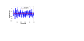
Figure 1: Estimates for $Q$ under 500 different scenarios

V Conclusions

The past few decades have witnessed much progress in optimal filtering for systems with arbitrary unknown inputs and stochastic noises. However, the existing works assume perfect knowledge of the noise covariances in the filter design, which is impractical. In this paper, for stochastic systems under unknown inputs, we have investigated the identifiability question of the process and measurement noises covariances (i.e., $Q$ and $R$) using the correlation-based measurement difference approach.

More specifically, we have focused on the single-step measurement case, and established (i) necessary conditions under which $Q$ and $R$ can be uniquely jointly identified (see Proposition 2); (ii) necessary and sufficient conditions under which $Q$ can be uniquely identified, when $R$ is known (see Proposition 3 and Corollary 1); (iii) necessary conditions under which $R$ can be uniquely identified, when $Q$ is known (see Proposition 4). Moreover, it has been shown that for achieving the results mentioned above, the measurement difference approach requires some decoupling conditions for constructing a stationary time series (see Proposition 1). The latter conditions are proved to be sufficient (see Theorem 1) for the strong detectability requirement in [11].

The above findings reveal that only under restrictive conditions, $Q$/$R$ can be potentially uniquely identified. This not only helps us to have a better understanding of the applicability of existing filtering frameworks under unknown inputs (since almost all of them require perfect knowledge of the noise covariances) but also calls for further investigation of alternative and more viable noise covariance methods under unknown inputs.

VI Acknowledgment

The authors would like to thank the reviewers and Editors for their constructive suggestions which have helped to improve the quality and presentation of this paper significantly. He Kong’s work was supported by the Science, Technology, and Innovation Commission of Shenzhen Municipality [Grant No. ZDSYS20200811143601004]. Tianshi Chen’s work was supported by the Thousand Youth Talents Plan funded by the central government of China, the Shenzhen Science and Technology Innovation Council under contract No. Ji-20170189, the President’s grant under contract No. PF. 01.000249 and the Start-up grant under contract No. 2014.0003.23 funded by the Chinese University of Hong Kong, Shenzhen.

References

- [1] A. Cristofaro and T. A. Johansen, Fault tolerant control allocation using unknown input observers, Automatica, Vol. 50, No. 7, pp. 1891–1897, 2014.
- [2] Z. Gao, X. Liu, and M. Chen, Unknown input observer based robust fault estimation for systems corrupted by partially-decoupled disturbances, IEEE Trans. on Industrial Electronics, Vol. 63, No. 4, pp. 2537–2547, 2016.
- [3] Y. Wang, D. Zhao, Y. Li, and S. X. Ding, Unbiased minimum variance fault and state estimation for linear discrete time-varying two-dimensional systems, IEEE Trans. on Automatic Control, Vol. 62, No. 10, pp. 5463–5469, 2017.
- [4] R. Ma, J. Fu, and T. Chai, Dwell-time-based observer design for unknown input switched linear systems without requiring strong detectability of subsystems, IEEE Trans. on Automatic Control, Vol. 62, No. 8, 4215–4221, 2017.
- [5] J. Qi, A. F. Taha, and J. Wang, Comparing Kalman filters and observers for power system dynamic state estimation with model uncertainty and malicious cyber attacks, IEEE Access, Vol. 6, pp. 77155–77168, 2018.
- [6] T. Yang, C. Murguia, M. Kuijper, and D. Nešić, An unknown input multi-observer approach for estimation and control under adversarial attacks, IEEE Trans. on Control of Network Systems, Vol. 8, No. 1, pp. 475–486, 2021.
- [7] H. Ohlsson, F. Gustafsson, L. Ljung, and S. Boyd, Smoothed state estimates under abrupt changes using sum-of-norms regularization, Automatica, Vol. 48, No. 4, pp. 595–605, 2012.
- [8] H. H. Alhelou, M. E. H. Golshan, and N. D. Hatziargyriou, Deterministic dynamic state estimation-based optimal LFC for interconnected power systems using unknown input observer, IEEE Trans. on Smart Grid, Vol. 11, No. 2, pp. 1582–1592, 2020.
- [9] J. Fu, R. Ma, and T. Chai, Finite-time stabilization of a class of uncertain nonlinear systems via logic-based switchings, IEEE Trans. on Automatic Control, Vol. 62, No. 11, 5998–6003, 2017.
- [10] L. Imsland, T. A. Johansen, H. F. Grip, and T. I. Fossen, On non-linear unknown input observers–applied to lateral vehicle velocity estimation on banked roads, International Journal of Control, Vol. 80, No. 11, pp. 1741–1750, 2007.
- [11] M. L. J. Hautus, Strong detectability and observers, Linear Algebra and Its Applications, Vol. 50, pp. 353–368, 1983.
- [12] M. Darouach, M. Zasadzinski, and M. Boutayeb, Extension of minimum variance estimation for systems with unknown inputs, Automatica, Vol. 39, No. 5, pp. 867–876, 2003.
- [13] S. Gillijns and B. De Moor, Unbiased minimum-variance input and state estimation for linear discrete-time systems with direct feedthrough, Automatica, Vol. 43, No. 5, pp. 934–937, 2007.
- [14] H. Fang and R. A. de Callafon, On the asymptotic stability of minimum-variance unbiased input and state estimation, Automatica, Vol. 48, No. 12, pp. 3183–3186, 2012.
- [15] S. Gillijns and B. De Moor, Unbiased minimum-variance input and state estimation for linear discrete-time systems, Automatica, Vol. 43, No. 1, pp. 111–116, 2007.
- [16] J. Su, B. Li, and W. H. Chen, On existence, optimality and asymptotic stability of the Kalman filter with partially observed inputs, Automatica, Vol. 53, pp. 149–154, 2015.
- [17] C. Hsieh, Extension of unbiased minimum-variance input and state estimation for systems with unknown inputs, Automatica, Vol. 45, No. 9, pp. 2149–2153, 2009.
- [18] Y. Cheng, H. Ye, Y. Wang, and D. Zhou, Unbiased minimum-variance state estimation for linear systems with unknown input, Automatica, Vol. 45, No. 2, pp. 485–491, 2009.
- [19] S. Z. Yong, M. Zhu, and E. Frazzoli, A unified filter for simultaneous input and state estimation of linear discrete-time stochastic systems, Automatica, Vol. 63, pp. 321–329, 2016.
- [20] R. R. Bitmead, M. Hovd, and M. A. Abooshahab, A Kalman-filtering derivation of simultaneous input and state estimation, Automatica, Vol. 108, 2019.
- [21] H. Kong and S. Sukkarieh, An internal model approach to estimation of systems with arbitrary unknown inputs, Automatica, Vol. 108, Art. 108482, pp. 1–11, 2019.
- [22] H. Kong, M. Shan, D. Su, Y. Qiao, A. Al-Azzawi, and S. Sukkarieh, Filtering for systems subject to unknown inputs without a priori initial information, Automatica, Vol. 120, Art. 109122, pp. 1–12, 2020.
- [23] J. Wakulicz, H. Kong, and S. Sukkarieh, Active information acquisition under arbitrary unknown disturbances, Proc. of IEEE Int. Conference on Robotics and Automation, pp. 8429–8435, 2021.
- [24] D. Yu and S. Chakravorty, A stochastic unknown input realization and filtering technique, Automatica, Vol. 63, No. 1, pp. 26–33, 2016.
- [25] H. Lan, Y. Liang, F. Yang, Z. Wang, and Q. Pan, Joint estimation and identification for stochastic systems with unknown inputs, IET Control Theory & Applications, Vol. 7, No. 10, pp. 1377–1386, 2013.
- [26] M. Gevers, A personal view of the development of system identification, IEEE Control Systems Magazine, Vol. 26, No. 6, pp. 93–105, 2006.
- [27] F. V. Lima and J. B. Rawlings, Nonlinear stochastic modeling to improve state estimation in process monitoring and control, AIChE Journal, Vol. 57, No. 4, pp. 996–1007, 2011.
- [28] M. Karasalo and X. Hu, An optimization approach to adaptive Kalman filtering, Automatica, Vol. 47, No. 8, pp. 1785–1793, 2011.
- [29] M. Ge and E. Kerrigan, Noise covariance identification for nonlinear systems using expectation maximization and moving horizon estimation, Automatica, Vol. 77, pp. 336–343, 2017.
- [30] J. Dunik, O. Straka, O. Kost, and J. Havlik, Noise covariance matrices in state-space models: A survey and comparison of estimation methods—Part I, International Journal of Adaptive Control and Signal Processing, Vol. 31, No. 11, pp. 1505–1543, 2017.
- [31] B. J. Odelson, M. R. Rajamani, and J. B. Rawlings, A new autocovariance least-squares method for estimating noise covariances, Automatica, Vol. 42, No. 2, pp. 303–308, 2006.
- [32] M. R. Rajamani and J. B. Rawlings, Estimation of the disturbance structure from data using semidefinite programming and optimal weighting, Automatica, Vol. 45, No. 1, pp. 142–148, 2009.
- [33] T. J. Arnold, Noise covariance estimation for linear systems, PhD thesis, Department of Chemical and Biological Engineering, The University of Wisconsin–Madison, USA, 2020.
- [34] B. Feng, M. Fu, H. Ma, Y. Xia, and B. Wang, Kalman filter with recursive covariance estimation–Sequentially estimating process noise covariance, IEEE Trans. on Industrial Electronics, Vol. 61, No. 11, pp. 6253–6263, 2014.
- [35] J. Dunik, O. Kost, and O. Straka, Design of measurement difference autocovariance method for estimation of process and measurement noise covariances, Automatica, Vol. 90, pp. 16–24, 2018.
- [36] R. Moghe, R. Zanetti, and M. R. Akella, Adaptive Kalman filter for detectable linear time-invariant systems, Journal of Guidance, Control, and Dynamics, Vol. 42, No. 10, pp. 2197–2205, 2019.
- [37] A. J. Laub, Matrix analysis for scientists and engineers, SIAM, 2005.
- [38] T. Chen and L. Ljung, Implementation of algorithms for tuning parameters in regularized least squares problems in system identification, Automatica, Vol. 49, No. 7, pp. 2213–2220, 2013.
- [39] M. Grant and S. Boyd, CVX: Matlab software for disciplined convex programming, version 2.0 beta, http://cvxr.com/cvx, 2013.