Asymptotically preserving particle methods for strongly magnetized plasmas in a torus

Abstract.

We propose and analyze a class of particle methods for the Vlasov equation with a strong external magnetic field in a torus configuration. In this regime, the time step can be subject to stability constraints related to the smallness of Larmor radius. To avoid this limitation, our approach is based on higher-order semi-implicit numerical schemes already validated on dissipative systems [3] and for magnetic fields pointing in a fixed direction [10, 11, 13]. It hinges on asymptotic insights gained in [12] at the continuous level. Thus, when the magnitude of the external magnetic field is large, this scheme provides a consistent approximation of the guiding-center system taking into account curvature and variation of the magnetic field. Finally, we carry out a theoretical proof of consistency and perform several numerical experiments that establish a solid validation of the method and its underlying concepts.

Keywords. High-order time discretization; Vlasov equation; Strong magnetic field; Particle methods.

1. Introduction

The main concern of the present paper is the study of plasma confined by a strong external nonconstant magnetic field, where the charged particles evolve under an electrostatic and intense confining magnetic field. This configuration is typical of a tokamak plasma [1, 22] where the magnetic field is used to confine particles inside the core of the device. Kinetic models, based on a mesoscopic description of the various particles constituting a plasma, and coupled to Maxwell’s equations for the computation of the electromagnetic fields, are very precise approaches for the study of such thermonuclear fusion plasmas Here we suppose that collective effects are dominant and the plasma is entirely modelled with transport equations, where the unknown is the number density of particles $f\equiv f(t,{\mathbf{x}},{\mathbf{v}})$ depending on time $t\geq 0$, position ${\mathbf{x}}\in\Omega\subset\mathbb{R}^{3}$ and velocity ${\mathbf{v}}\in\mathbb{R}^{3}$. The transport equation is written in adimensional form as

(1.1) $$\partial_{t}f^{\varepsilon}\,+\,\textrm{div}_{\mathbf{x}}(f^{\varepsilon}\,{\mathbf{v}})\,+\,\textrm{div}_{\mathbf{v}}\left(f^{\varepsilon}\,\left(\frac{{\mathbf{v}}\wedge{\mathbf{B}}(t,{\mathbf{x}})}{\varepsilon}\,+\,{\mathbf{E}}(t,{\mathbf{x}})\right)\right)\,=\,0\,,$$

where the parameter $\varepsilon$ accounts for the high intensity of the external magnetic field, $1/\varepsilon$ being related to the so-called gyro-frequency. The characteristic flow associated to this transport equation is encoded by the following ODEs

(1.2) $$\left\{\begin{array}[]{l}\displaystyle\frac{\operatorname{d}{\mathbf{x}}}{\operatorname{d}t}\,=\,{\mathbf{v}}\,,\\[8.99994pt] \displaystyle\frac{\operatorname{d}{\mathbf{v}}}{\operatorname{d}t}\,=\,\frac{{\mathbf{v}}\wedge{\mathbf{B}}(t,{\mathbf{x}})}{\varepsilon}\,+\,{\mathbf{E}}(t,{\mathbf{x}})\,,\end{array}\right.$$

where $\wedge$ denotes the standard vector product on $\mathbb{R}^{3}$, ${\mathbf{B}}$ stands for the external magnetic field, ${\mathbf{E}}$ for an electric field, either external or obtained by solving a field equation. This kinetic equation provides an appropriate description of turbulent transport in a general context, but it also requires to solve a high dimensional problem which leads to a huge computational cost. One approach consists in reducing the cost of numerical simulations, by deriving asymptotic models with a smaller number of variables than the kinetic description. Indeed, large magnetic fields usually lead to the so-called drift-kinetic limit [19, 18]. We refer to [17, 21, 20] and [12] for a detailed account of mathematical results on this topic and relevant entering gates to the extensive physical literature. Besides those, on the physical side, we only point out [4], as posterior to the references that may found there, and closer to, but distinct from, [12] that inspires the numerical methods introduced in the present contribution.

Other approaches are based on the construction of efficient particle solvers for the original dynamics, to be used as a piece of a PIC scheme. Over the last decade, considerable efforts have been devoted to the design of such solvers and we refer the reader to [2, 24, 9, 27, 10, 11, 14, 6, 7, 23, 15, 25, 13, 26, 16, 8] for both significant contributions and relevant entering gates to the now abundant literature. Along these years, roughly speaking, two kind of goals were assigned to the built numerical schemes. On one hand, one may wish to enforce the preservation of some of the geometrical structures of the original system (symplecticity, conservation of the total energy, or of a momentum associated with some group of symmetry,…). On the other hand, one may try to ensure that the designed schemes are consistent with the above-mentioned asymptoptic reduction, or at least with some of its consequences (approximate conservation of adiabatic invariants, effective spatial drifts,…). Schemes satisfying (some of) the former conditions are typically called structure preserving schemes, whereas those satisfying a version of the latter are named asymptotic preserving. Note that the asymptotic preserving property includes that in the limit $\varepsilon\rightarrow 0$, schemes do capture accurately the non stiff part of the evolution while allowing for coarse discretization parameters.

A feature of the present evolution, or more generally of rapidly oscillating dynamics, that makes it difficult to capture numerically is that the two kinds of requirement may lead to conflicting choices. Indeed, an apparent paradox to solve is that, in the regime when $\varepsilon$ is small and $({\mathbf{x}},{\mathbf{v}})$ solve (1.2), the transverse microscopic kinetic energy $\|{\mathbf{v}}_{\perp}\|^{2}/2$, entering in many conserved quantities, evolves slowly and remains of size $1$ whereas the transverse velocity ${\mathbf{v}}_{\perp}$, that is, the part of the velocity orthogonal to ${\mathbf{B}}$, converges (weakly) to an effective drift of size $\varepsilon$, by rapidly oscillating about it, the latter oscillatory convergence being the core of the gyro-kinetic asymptotic reduction. For this reason, many of the structure preserving schemes built with classical tools from geometric numerical integration, such as multi-step schemes [14], variational schemes [27, 15, 25], or splitting schemes [26], fail to capture accurately the correct asymptotic behavior, and, even worse, many of them are only known to provide the desired structure preservation under upper size constraints on $\Delta t/\varepsilon$, $\Delta t$ denoting the numerical time step. Unfortunately, so far proposed fixes for these geometric schemes, such as the introduction of $\varepsilon$-dependent filters [16], are consistent with the exact dynamics, as $\Delta t$ goes to zero, only under lower size restrictions on $\Delta t/\sqrt{\varepsilon}$ so that for the moment none of these provide a satisfactory behavior for the whole range of relevant physical and numerical parameters.

A much less standard class of schemes developed in [6, 7], consists of explicitly doubling time variables, going from $(t,{\mathbf{x}},{\mathbf{v}})$ to $(t,\tau,{\mathbf{x}},{\mathbf{v}})$, where $\tau$ is a periodic time, the original system being recovered at the $\varepsilon$-diagonal $(t,\tau)=(t,t/\varepsilon)$. The corresponding methods are extremely good at capturing oscillations, and some of them do preserve parts of the relevant geometric structures. Yet their design requires a deep a priori understanding of the detailed structure of oscillations and they seem hard to implement efficiently and to combine with standard field solvers used to compute electromagnetic fields.

The class of semi-implicit schemes proposed in [10, 11, 13] focuses on the less ambitious goal of guaranteeing only the asymptotic preserving property, thus the recovering of both the exact dynamics as $\Delta t$ goes to zero, uniformly with respect to $\varepsilon$, and the slow reduced dynamics, including the guiding-center particle motion, when $\varepsilon$ goes to zero, uniformly with respect to $\Delta t$. We stress that by many respects those schemes are remarkably natural and simple, and may easily be inserted in a standard PIC code. For complex geometries, our schemes are designed as high-order semi-implicit schemes [3] applied to an augmented formulation. Our supporting strategy is quite systematic and versatile, but so far we have implemented it only for homogeneous magnetic fields [10, 13] and magnetic fields pointing in a fixed direction [11].

Incidentally, we point out that similar restrictions hold for all the schemes described so far, in the sense that mathematical guarantees for asymptotic preservation have been provided only for magnetic fields pointing in a fixed direction, as in [11], and for magnetic fields with a homogeneous intensity, that is, with $\|{\mathbf{B}}\|$ constant, as in [7]. The former configuration precludes magnetic curvature drifts, that are notoriously difficult to capture, whereas the latter ensure that particles share the same period thus remain synchronized, a situation much easier to analyze with filtering or averaging techniques.

In the present article, we show how our approach may be extended to genuinely three dimensional magnetic fields, with symmetries of a torus configuration. The geometric framework is thought as a toy model, mimicking realistic configurations used in tokamak devices. However we restrain from designing schemes that provide a second-order description of the full slow dynamics (as in [11]) so as to gain, in the trade-off, a structure preservation property, the approximate conservation of the total energy, but also to maintain the complexity of the designed schemes to a bare minimum. With this respect, our present goals are similar to those underlying the design of the fully-implicit numerical schemes in [23, 8].

The rest of the paper is organized as follows. In Section 2, we present the geometric framework of our study and reformulate the equation of motion (1.2) in order to identify carefully fast and slow scales. In Section 3, we derive the expected asymptotic behavior in the regime $\varepsilon\ll 1$ by applying, at the continuous level, the arguments devised in [12]. Then in Section 4, we present several time discretization techniques and we prove uniform consistency of the schemes in the limit $\varepsilon\rightarrow 0$. Finally, Section 5 is then devoted to numerical simulations of particle motion in various regimes, including $\varepsilon\approx 1$ and $\varepsilon\ll 1$.

2. Toroidal configuration

Firstly, we identify adapted coordinates. Hence, we pick some radius $R_{0}>0$ for the torus and introduce toroidal coordinates through ${\mathbf{x}}={\mathbf{X}}(r,\theta,\varphi)$, where

$${\mathbf{X}}(r,\theta,\varphi)\,=\,\left(\begin{array}[]{l}R(r,\theta)\cos(\varphi)\\[8.99994pt] R(r,\theta)\sin(\varphi)\\[8.99994pt] r\sin(\theta)\end{array}\right),$$

with $R(r,\theta):=R_{0}+r\cos(\theta)$ and $(r,\theta,\varphi)$ varying in $(0,R_{0})\times(\mathbb{R}/2\pi\mathbb{Z})\times(\mathbb{R}/2\pi\mathbb{Z})$. To prepare the corresponding change of variables for the velocity we also introduce the orthonormal basis $(\operatorname{\mathbf{e}}_{r},\operatorname{\mathbf{e}}_{\theta},\operatorname{\mathbf{e}}_{\varphi})$ by

$$\left\{\begin{array}[]{ll}\operatorname{\mathbf{e}}_{r}(\theta,\varphi)&=(\cos(\theta)\,\cos(\varphi),\,\cos(\theta)\,\sin(\varphi),\,\sin(\theta))\,,\\[8.99994pt] \operatorname{\mathbf{e}}_{\theta}(\theta,\varphi)&=(-\sin(\theta)\,\cos(\varphi),\,-\sin(\theta)\,\sin(\varphi),\,\cos(\theta))\,,\\[8.99994pt] \operatorname{\mathbf{e}}_{\varphi}(\varphi)&=(-\sin(\varphi),\,\cos(\varphi),\,0)\,.\end{array}\right.$$

Then we replace original coordinates $({\mathbf{x}},{\mathbf{v}})$ with $(r,\theta,\varphi,v_{r},v_{\theta},v_{\varphi})$ where

$$v_{\alpha}=\langle{\mathbf{v}},\operatorname{\mathbf{e}}_{\alpha}\rangle,\quad{\rm for}\quad\alpha\in\{r,\,\theta,\,\varphi\}$$

In the new coordinates, the equations of motion (1.2) become

(2.1) $$\left\{\begin{array}[]{l}\displaystyle\frac{\operatorname{d}r}{\operatorname{d}t}\,=\,v_{r}\,,\hskip 20.00003ptr\,\frac{\operatorname{d}\theta}{\operatorname{d}t}\,=\,v_{\theta}\,,\hskip 20.00003ptR(r,\theta)\,\frac{\operatorname{d}\varphi}{\operatorname{d}t}\,=\,v_{\varphi}\,,\\[8.99994pt] \displaystyle\frac{\operatorname{d}v_{r}}{\operatorname{d}t}\,=\,\frac{v_{\varphi}\,B_{\theta}-v_{\theta}\,B_{\varphi}}{\varepsilon}\,+\,E_{r}\,+\,\frac{v_{\theta}^{2}}{r}\,+\,\cos(\theta)\,\frac{v_{\varphi}^{2}}{R},\\[8.99994pt] \displaystyle\frac{\operatorname{d}v_{\theta}}{\operatorname{d}t}\,=\,\frac{v_{r}\,B_{\varphi}-v_{\varphi}\,B_{r}}{\varepsilon}\,+\,E_{\theta}\,-\,\frac{v_{r}\,v_{\theta}}{r}\,-\,\sin(\theta)\,\frac{v_{\varphi}^{2}}{R},\\[8.99994pt] \displaystyle\frac{\operatorname{d}v_{\varphi}}{\operatorname{d}t}\,=\,\frac{v_{\theta}\,B_{r}-v_{r}\,B_{\theta}}{\varepsilon}\,+\,E_{\varphi}\,-\,\cos(\theta)\,\frac{v_{r}\,v_{\varphi}}{R}\,+\,\sin(\theta)\,\frac{v_{\theta}\,v_{\varphi}}{R},\end{array}\right.$$

where consistently we have set

$$E_{\alpha}\,=\,\langle{\mathbf{E}},\operatorname{\mathbf{e}}_{\alpha}\rangle,\qquad B_{\alpha}\;=\;\langle{\mathbf{B}},\operatorname{\mathbf{e}}_{\alpha}\rangle,\quad{\rm for}\quad\alpha\in\{r,\varphi,\theta\}.$$

Now we make the assumption that the magnetic field is steady and axi-symmetric, that is, that the magnetic field components $(B_{r},B_{\varphi},B_{\theta})$ do not depend on $t$ and $\varphi$. Moreover we also assume that magnetic field lines are contained in $r$ level surfaces, that is, that $B_{r}\equiv 0$. Hence the magnetic field ${\mathbf{B}}$ takes the form

(2.2) $${\mathbf{B}}(r,\theta,\varphi)=b(r,\theta)\operatorname{\mathbf{e}}_{\mkern 3.0mu\vphantom{\perp}\vrule depth=0.0pt\mkern 2.0mu\vrule depth=0.0pt\mkern 3.0mu}(r,\theta,\varphi)$$

with $b$ positive-valued and the unit vector $\operatorname{\mathbf{e}}_{\mkern 3.0mu\vphantom{\perp}\vrule depth=0.0pt\mkern 2.0mu\vrule depth=0.0pt\mkern 3.0mu}$ defined by

(2.3) $$\operatorname{\mathbf{e}}_{\mkern 3.0mu\vphantom{\perp}\vrule depth=0.0pt\mkern 2.0mu\vrule depth=0.0pt\mkern 3.0mu}(r,\theta,\varphi)\,=\,\cos(\omega)\,\operatorname{\mathbf{e}}_{\varphi}(\varphi)\,+\,\sin(\omega)\,\operatorname{\mathbf{e}}_{\theta}(\theta,\varphi)\,,$$

where $\omega$ is a real valued function depending only on $(r,\theta)$.

There are two key features in the present form of ${\mathbf{B}}$. On one hand, in suitable coordinates, the dependence on the angle $\varphi$ of the dynamics of other variables occurs only through the possible non axi-symmetry of the electric field ${\mathbf{E}}$. On the other hand, independently of any further assumption on $\omega$, magnetic field lines are everywhere orthogonal to $\operatorname{\mathbf{e}}_{r}$. In particular, introducing $\operatorname{\mathbf{e}}_{\perp}$ through

(2.4) $$\operatorname{\mathbf{e}}_{\perp}(r,\theta,\varphi)\,=\,\sin(\omega)\,\operatorname{\mathbf{e}}_{\varphi}(\varphi)\,-\,\cos(\omega)\,\operatorname{\mathbf{e}}_{\theta}(\theta,\varphi)\,,$$

one obtains $(\operatorname{\mathbf{e}}_{r},\operatorname{\mathbf{e}}_{\perp},\operatorname{\mathbf{e}}_{\mkern 3.0mu\vphantom{\perp}\vrule depth=0.0pt\mkern 2.0mu\vrule depth=0.0pt\mkern 3.0mu})$ valued in direct orthonormal bases.

Remark 2.1.

The analysis of [12] applies to an arbitrary geometry and, in principal, the corresponding numerical approach described here could be used in such a generality. Yet, in full generality, some of the involved computations turn out to be rather cumbersome. We use axi-symmetry and the orthogonality of $\operatorname{\mathbf{e}}_{r}$ and ${\mathbf{B}}$ to simplify the latter. We would like to point out a simple way to relax the latter assumption so as to include concrete applications without dramatically increasing computational complexity. On one hand, at a similar price, one may replace $(r,\theta)$ with another set of two-dimensional coordinates $(\psi,\chi)$ generating an orthonormal frame $(\operatorname{\mathbf{e}}_{\psi},\operatorname{\mathbf{e}}_{\chi},\operatorname{\mathbf{e}}_{\varphi})$ such that $\operatorname{\mathbf{e}}_{\psi}$ and ${\mathbf{B}}$ are orthogonal. This allows to treat geometries that are axi-symmetric toroidal-like.

Therefore, since the leading-order dynamics is a rotation of the velocity in the plane orthogonal to $\operatorname{\mathbf{e}}_{\mkern 3.0mu\vphantom{\perp}\vrule depth=0.0pt\mkern 2.0mu\vrule depth=0.0pt\mkern 3.0mu}$, it is convenient to use for ${\mathbf{v}}$ a frame adapted to $\operatorname{\mathbf{e}}_{\mkern 3.0mu\vphantom{\perp}\vrule depth=0.0pt\mkern 2.0mu\vrule depth=0.0pt\mkern 3.0mu}$, and we shall use $(\operatorname{\mathbf{e}}_{r},\operatorname{\mathbf{e}}_{\perp},\operatorname{\mathbf{e}}_{\mkern 3.0mu\vphantom{\perp}\vrule depth=0.0pt\mkern 2.0mu\vrule depth=0.0pt\mkern 3.0mu})$ to provide such a frame. Accordingly we introduce

$$v_{\alpha}\,=\,\langle{\mathbf{v}},\operatorname{\mathbf{e}}_{\alpha}\rangle,\qquad E_{\alpha}\,=\,\langle{\mathbf{E}},\operatorname{\mathbf{e}}_{\alpha}\rangle,\quad{\rm for}\quad\alpha\in\{r,\perp,{\mkern 3.0mu\vphantom{\perp}\vrule depth=0.0pt\mkern 2.0mu\vrule depth=0.0pt\mkern 3.0mu}\}$$

and

$${\mathbf{v}}_{\perp} =(v_{r},v_{\perp})\,, {\mathbf{E}}_{\perp} =(E_{r},E_{\perp})\,.$$

Therefore from the definition of $(\operatorname{\mathbf{e}}_{\mkern 3.0mu\vphantom{\perp}\vrule depth=0.0pt\mkern 2.0mu\vrule depth=0.0pt\mkern 3.0mu},\operatorname{\mathbf{e}}_{\perp})$ in (2.3) and (2.4), we notice that

(2.5) $$\left\{\begin{array}[]{l}v_{\mkern 3.0mu\vphantom{\perp}\vrule depth=0.0pt\mkern 2.0mu\vrule depth=0.0pt\mkern 3.0mu}\,=\,\cos(\omega)\,v_{\varphi}\,+\,\sin(\omega)\,v_{\theta},\\[8.99994pt] v_{\perp}\,=\,\sin(\omega)\,v_{\varphi}\,-\,\cos(\omega)\,v_{\theta}\end{array}\right.$$

and conversely,

$$\left\{\begin{array}[]{l}v_{\varphi}\,=\,\cos(\omega)\,v_{\mkern 3.0mu\vphantom{\perp}\vrule depth=0.0pt\mkern 2.0mu\vrule depth=0.0pt\mkern 3.0mu}\,+\,\sin(\omega)\,v_{\perp},\\[8.99994pt] v_{\theta}\,=\,\sin(\omega)\,v_{\mkern 3.0mu\vphantom{\perp}\vrule depth=0.0pt\mkern 2.0mu\vrule depth=0.0pt\mkern 3.0mu}\,-\,\cos(\omega)\,v_{\perp}.\end{array}\right.$$

Hence we may now write System (1.2) in terms of $(r,\theta,\varphi,{\mathbf{v}}_{\perp},v_{\mkern 3.0mu\vphantom{\perp}\vrule depth=0.0pt\mkern 2.0mu\vrule depth=0.0pt\mkern 3.0mu})$ as,

(2.6) $$\frac{\operatorname{d}}{\operatorname{d}t}\begin{pmatrix}r\\[8.99994pt] \varphi\\[8.99994pt] \theta\end{pmatrix} \,=\,\begin{pmatrix}v_{r}\\[8.99994pt] \displaystyle\frac{\cos(\omega)\,v_{\mkern 3.0mu\vphantom{\perp}\vrule depth=0.0pt\mkern 2.0mu\vrule depth=0.0pt\mkern 3.0mu}\,+\,\sin(\omega)\,v_{\perp}}{R}\\[8.99994pt] \displaystyle\frac{\sin(\omega)\,v_{\mkern 3.0mu\vphantom{\perp}\vrule depth=0.0pt\mkern 2.0mu\vrule depth=0.0pt\mkern 3.0mu}\,-\,\cos(\omega)\,v_{\perp}}{r}\end{pmatrix}\,,$$

whereas the equation for $v_{\mkern 3.0mu\vphantom{\perp}\vrule depth=0.0pt\mkern 2.0mu\vrule depth=0.0pt\mkern 3.0mu}$ is obtained using (2.1) and (2.5),

$$\frac{\operatorname{d}v_{\mkern 3.0mu\vphantom{\perp}\vrule depth=0.0pt\mkern 2.0mu\vrule depth=0.0pt\mkern 3.0mu}}{\operatorname{d}t} = -v_{\perp}\,\left(\partial_{r}\omega\,v_{r}\,+\frac{\partial_{\theta}\omega}{r}\,v_{\theta}\right)\,+\,\cos(\omega)\frac{\operatorname{d}v_{\varphi}}{\operatorname{d}t}\,+\,\sin(\omega)\,\frac{\operatorname{d}v_{\theta}}{\operatorname{d}t}$$

$$= -v_{\perp}\,\left(\partial_{r}\omega\,v_{r}\,+\frac{\partial_{\theta}\omega}{r}\,v_{\theta}\right)\,+\,E_{\mkern 3.0mu\vphantom{\perp}\vrule depth=0.0pt\mkern 2.0mu\vrule depth=0.0pt\mkern 3.0mu}\,-\,\frac{\sin(\theta)}{R}\,v_{\varphi}\,v_{\perp}$$

$$-\,v_{r}\,\left(\frac{\cos(\theta)}{R}\,\cos(\omega)\,v_{\varphi}\,+\,\frac{1}{r}\,\sin(\omega)\,v_{\theta}\right).$$

Then replacing $(v_{\theta},v_{\varphi})$ with their expression with respect to $(v_{\mkern 3.0mu\vphantom{\perp}\vrule depth=0.0pt\mkern 2.0mu\vrule depth=0.0pt\mkern 3.0mu},v_{\perp})$ yields

(2.7) $$\left\{\begin{array}[]{l}\displaystyle\frac{\operatorname{d}v_{\mkern 3.0mu\vphantom{\perp}\vrule depth=0.0pt\mkern 2.0mu\vrule depth=0.0pt\mkern 3.0mu}}{\operatorname{d}t}\,=\,E_{\mkern 3.0mu\vphantom{\perp}\vrule depth=0.0pt\mkern 2.0mu\vrule depth=0.0pt\mkern 3.0mu}+F_{\mkern 3.0mu\vphantom{\perp}\vrule depth=0.0pt\mkern 2.0mu\vrule depth=0.0pt\mkern 3.0mu},\\[8.99994pt] \displaystyle\textrm{with }\qquad F_{\mkern 3.0mu\vphantom{\perp}\vrule depth=0.0pt\mkern 2.0mu\vrule depth=0.0pt\mkern 3.0mu}\,:=\,\gamma\,v_{\mkern 3.0mu\vphantom{\perp}\vrule depth=0.0pt\mkern 2.0mu\vrule depth=0.0pt\mkern 3.0mu}\,v_{r}\,+\,\alpha\,v_{\mkern 3.0mu\vphantom{\perp}\vrule depth=0.0pt\mkern 2.0mu\vrule depth=0.0pt\mkern 3.0mu}\,v_{\perp}\,+\,\left(\delta-\partial_{r}\omega\right)\,v_{\perp}\,v_{r}\,+\,\beta\;v_{\perp}^{2}\end{array}\right.$$

where the parameters $\alpha$, $\beta$, $\gamma$ and $\delta$ depend only on $(r,\theta)$,

(2.8) $$\left\{\begin{array}[]{l}\displaystyle\alpha\,=\,-\frac{\partial_{\theta}\omega}{r}\,\sin(\omega)\,-\,\frac{\sin(\theta)}{R}\,\cos(\omega)\,,\\[8.99994pt] \displaystyle\beta\,=\,\frac{\partial_{\theta}\omega}{r}\,\cos(\omega)\,-\,\frac{\sin(\theta)}{R}\,\sin(\omega)\,,\\[8.99994pt] \displaystyle\gamma\,=\,-\frac{\sin^{2}(\omega)}{r}\,-\,\frac{\cos(\theta)}{R}\,\cos^{2}(\omega)\,,\\[8.99994pt] \displaystyle\delta\,=\,-\left(\frac{\cos(\theta)}{R}\,-\,\frac{1}{r}\right)\,\sin(\omega)\cos(\omega)\,.\end{array}\right.$$

Likewise, we obtain an equation for ${\mathbf{v}}_{\perp}=(v_{r},v_{\perp})$ as

(2.9) $$\left\{\begin{array}[]{l}\displaystyle\frac{\operatorname{d}v_{r}}{\operatorname{d}t}\,=\,E_{r}\,+\,C_{r}\,+\,\frac{b\,v_{\perp}}{\varepsilon}\,,\\[8.99994pt] \displaystyle\frac{\operatorname{d}v_{\perp}}{\operatorname{d}t}\,=\,E_{\perp}\,+\,C_{\perp}\,-\,\frac{b\,v_{r}}{\varepsilon}\,,\end{array}\right.$$

where ${\mathbf{C}}_{\perp}=(C_{r},C_{\perp})$,

$$\left\{\begin{array}[]{l}\displaystyle C_{r}\,:=\,-\gamma\,v_{\mkern 3.0mu\vphantom{\perp}\vrule depth=0.0pt\mkern 2.0mu\vrule depth=0.0pt\mkern 3.0mu}^{2}\,-\,2\,\delta\,v_{\mkern 3.0mu\vphantom{\perp}\vrule depth=0.0pt\mkern 2.0mu\vrule depth=0.0pt\mkern 3.0mu}\,v_{\perp}\,+\,\zeta\,v_{\perp}^{2}\,,\\[8.99994pt] \displaystyle C_{\perp}\,:=\,-\alpha\,v_{\mkern 3.0mu\vphantom{\perp}\vrule depth=0.0pt\mkern 2.0mu\vrule depth=0.0pt\mkern 3.0mu}^{2}\,+\,\left(\partial_{r}\omega+\delta\right)\,v_{\mkern 3.0mu\vphantom{\perp}\vrule depth=0.0pt\mkern 2.0mu\vrule depth=0.0pt\mkern 3.0mu}\,v_{r}\,-\,\beta\,v_{\mkern 3.0mu\vphantom{\perp}\vrule depth=0.0pt\mkern 2.0mu\vrule depth=0.0pt\mkern 3.0mu}\,v_{\perp}\,-\,\zeta\,v_{r}\,v_{\perp}\end{array}\right.$$

and

(2.10) $$\zeta\,=\,\frac{\cos^{2}(\omega)}{r}\,+\,\frac{\cos(\theta)}{R}\,\sin^{2}(\omega)\,.$$

This formulation allows to split the parallel and perpendicular directions with respect to the magnetic field. In particular, we get that at leading-order ${\mathbf{v}}_{\perp}$ is oscillating at a frequency of order $1/\varepsilon$ whereas $(r,\theta,\varphi,v_{\mkern 3.0mu\vphantom{\perp}\vrule depth=0.0pt\mkern 2.0mu\vrule depth=0.0pt\mkern 3.0mu})$ exhibit a slower dynamics. Furthermore, it allows to identify another slow variable $\|{\mathbf{v}}_{\perp}\|^{2}$, hence we introduce the new variable $b\mu\,:=\,{\|{\mathbf{v}}_{\perp}\|^{2}}/{2}$ and write its slow dynamic from (2.9) as

(2.11) $$\frac{\operatorname{d}b\mu}{\operatorname{d}t}\,=\,\langle{\mathbf{E}}_{\perp},\,{\mathbf{v}}_{\perp}\rangle\,-\,v_{\mkern 3.0mu\vphantom{\perp}\vrule depth=0.0pt\mkern 2.0mu\vrule depth=0.0pt\mkern 3.0mu}\,F_{\mkern 3.0mu\vphantom{\perp}\vrule depth=0.0pt\mkern 2.0mu\vrule depth=0.0pt\mkern 3.0mu}\,.$$

Note that our convoluted notation $b\,\mu$ is chosen to respect standard notational conventions of the physical literature devoted to gyro-kinetic reductions; see the related discussion in [12].

Our final step is motivated by the simple observation that when deriving asymptotic models the stiff part of (2.9) is used to replace, in the equations of slower components, ${\mathbf{v}}_{\perp}$ with slower or lower-order terms. To prepare such eliminations, it is convenient to divide System (2.9) by $b$. This hints at the introduction of the new variable

$${\mathbf{u}}_{\perp}=\frac{{\mathbf{v}}_{\perp}}{b}.$$

As a side effect, this will exhibit the effects of the gradients of the intensity of the magnetic field $b$ on the reduced asymptotic dynamics. With ${\mathbf{u}}_{\perp}$ in hands, we observe that (2.9) may be replaced with

(2.12) $$\left\{\begin{array}[]{l}\displaystyle\varepsilon\,\frac{\operatorname{d}u_{r}}{\operatorname{d}t}\,=\,\varepsilon\,\frac{E_{r}+C_{r}+G_{r}}{b}\,+\,v_{\perp}\,,\\[8.99994pt] \displaystyle\varepsilon\,\frac{\operatorname{d}u_{\perp}}{\operatorname{d}t}\,=\,\varepsilon\,\frac{E_{\perp}+C_{\perp}+G_{\perp}}{b}\,-\,v_{r}\,,\end{array}\right.$$

where ${\mathbf{G}}_{\perp}=(G_{r},G_{\perp})$ is given by

$$\left\{\begin{array}[]{l}\displaystyle G_{r}\,:=\,\eta\,v_{r}\,v_{\mkern 3.0mu\vphantom{\perp}\vrule depth=0.0pt\mkern 2.0mu\vrule depth=0.0pt\mkern 3.0mu}\,+\,\kappa\,v_{r}\,v_{\perp}\,+\,\lambda\,v_{r}^{2},\\[8.99994pt] \displaystyle G_{\perp}\,:=\,\eta\,v_{\mkern 3.0mu\vphantom{\perp}\vrule depth=0.0pt\mkern 2.0mu\vrule depth=0.0pt\mkern 3.0mu}\,v_{\perp}\,+\,\lambda\,v_{r}\,v_{\perp}\,+\,\kappa\,v_{\perp}^{2}\end{array}\right.$$

and $(\alpha,\beta,\gamma,\delta)$ is defined in (2.8) and the triplet $(\eta,\kappa,\lambda)$ is

(2.13) $$\left\{\begin{array}[]{l}\displaystyle\eta\,=\,-\frac{\sin(\omega)}{r}\,\frac{\partial_{\theta}b}{b},\\[8.99994pt] \displaystyle\kappa\,=\,\frac{\cos(\omega)}{r}\,\frac{\partial_{\theta}b}{b},\\[8.99994pt] \displaystyle\lambda\,=\,-\frac{\partial_{r}b}{b}.\end{array}\right.$$

In (2.12), ${\mathbf{E}}_{\perp}$ takes into account the effects of the electric field, whereas ${\mathbf{C}}_{\perp}$ describes the curvature effects and ${\mathbf{G}}_{\perp}$ those of the gradient of the magnetic field intensity. Let us observe that the structure of (2.6)-(2.13) strongly echoes the one of the two-dimensional inhomogeneous situation dealt with in [11], with ${\mathbf{v}}_{\perp}$ playing the role of the two-dimensional velocity and $(r,\theta,\varphi,v_{\mkern 3.0mu\vphantom{\perp}\vrule depth=0.0pt\mkern 2.0mu\vrule depth=0.0pt\mkern 3.0mu},b\,\mu)$ playing the role of the spatial position and the microscopic kinetic energy.

To prepare further manipulations, we write (2.12) in a more compact form as

(2.14) $${\mathbf{v}}_{\perp}\,=\,\varepsilon\,{\mathbf{U}}_{\perp}\,\,-\,\varepsilon\frac{\operatorname{d}\,}{\operatorname{d}t}\left({\mathbf{J}}_{0}{\mathbf{u}}_{\perp}\right)\,,$$

where

$${\mathbf{J}}_{0}\,:=\,\begin{pmatrix}0&1\\ -1&0\end{pmatrix}\,,$$

and

(2.15) $${\mathbf{U}}_{\perp}:=\frac{{\mathbf{J}}_{0}}{b}\left({\mathbf{E}}_{\perp}\,+\,{\mathbf{C}}_{\perp}\,+\,{\mathbf{G}}_{\perp}\right).$$

3. Asymptotic dynamics

We now consider the asymptotic regime $\varepsilon\ll 1$. When doing so, our focus is two-fold. On one hand, we are interested in the identification of the asymptotic reduction by itself, so as to know what are the objectives for the numerical schemes introduced below. On the other hand, we are also interested in unraveling the algebraic identities that supports the asymptotic reduction, since a convenient way to ensure that the asymptotic reduction takes also place at the discrete level is precisely to enforce discrete counterparts to such identities in the numerical schemes.

We could adapt or apply the arguments of [12] and obtain a fully rigorous mathematical analysis. Yet this would lead us too far beyond the main scope of the present paper. Instead, we borrow mostly the algebraic part of [12].

3.1. First order asymptotics

To begin with, as in [12, Lemmas 3.3 & 4.3], we observe that Equation (2.14) may be combined with slower equations to eliminate not only ${\mathbf{v}}_{\perp}$ but any expression linear in ${\mathbf{v}}_{\perp}$ with dependence on time and slow variables. Indeed if $t\mapsto{\mathcal{L}}(t)$ is a smooth map valued in a space of linear operators, there exist two functions $(\chi_{\mathbf{L}},\eta_{\mathbf{L}})\in L^{\infty}_{t}$ such that the equations of motion imply

(3.16) $${\mathbf{L}}\,{\mathbf{v}}_{\perp}\,=\,-\varepsilon\,\frac{\operatorname{d}\chi_{\mathbf{L}}}{\operatorname{d}t}\,+\,\varepsilon\,\eta_{\mathbf{L}}\,.$$

In particular, from this one expects that ${\mathbf{L}}\,{\mathbf{v}}_{\perp}$ converge to zero when $\varepsilon$ tends to zero in some sense. The underlying algebra is completely constructive but we refrain from giving it wherever it is not strictly needed.

Now we show how to apply the foregoing first principles to the study of the asymptotic dynamics of the slow variables $(r,\theta,\varphi,v_{\mkern 3.0mu\vphantom{\perp}\vrule depth=0.0pt\mkern 2.0mu\vrule depth=0.0pt\mkern 3.0mu},b\mu)$.

The dependence of System (2.6) on ${\mathbf{v}}_{\perp}$ is linear so that the foregoing argument is sufficient to reveal the first order part of it. We begin with the study of the time derivative of the variable $r$. Here the algebraic manipulation consists in using the second equation of (2.12) so as to eliminate the right hand side $v_{r}$ in (2.6). In this way, one derives

$$\frac{\operatorname{d}\,}{\operatorname{d}t}\left(r+\varepsilon\,\frac{v_{\perp}}{b}\right)\,=\,\varepsilon\,\frac{E_{\perp}+C_{\perp}}{b}+\varepsilon\,\left(v_{r}\frac{\partial_{r}b}{b}+\left(v_{\perp}\cos(\omega)+v_{\mkern 3.0mu\vphantom{\perp}\vrule depth=0.0pt\mkern 2.0mu\vrule depth=0.0pt\mkern 3.0mu}\sin(\omega)\right)\,\frac{\partial_{\theta}b}{b\,r}\right)\,\frac{v_{\perp}}{b},$$

which suggests that $r$ converges to the constant $r(0)$ when $\varepsilon$ tends to zero. We proceed in the same manner for the angle variables $(\varphi,\theta)$ using the property (3.16) to study the asymptotic behavior of linear terms with respect to ${\mathbf{v}}_{\perp}$. It gives that, for some $(\chi_{\varphi},\eta_{\varphi})$ and $(\chi_{\theta},\eta_{\theta})$,

$$\frac{\operatorname{d}}{\operatorname{d}t}\left(\varphi\,+\,\varepsilon\,\chi_{\varphi}\right)\,=\,\frac{\cos(\omega)\,v_{\mkern 3.0mu\vphantom{\perp}\vrule depth=0.0pt\mkern 2.0mu\vrule depth=0.0pt\mkern 3.0mu}}{R}\,+\,\varepsilon\,\eta_{\varphi}$$

and

$$\frac{\operatorname{d}}{\operatorname{d}t}\left(\theta\,+\,\varepsilon\,\chi_{\theta}\right)\,=\,\frac{\sin(\omega)\,v_{\mkern 3.0mu\vphantom{\perp}\vrule depth=0.0pt\mkern 2.0mu\vrule depth=0.0pt\mkern 3.0mu}}{r}\,+\,\varepsilon\,\eta_{\theta},$$

allowing to characterize the limit equation on $(\varphi,\theta)$. when $\varepsilon\rightarrow 0$.

Note that the equation for $v_{\mkern 3.0mu\vphantom{\perp}\vrule depth=0.0pt\mkern 2.0mu\vrule depth=0.0pt\mkern 3.0mu}$ given in (2.7) contains both linear and quadratic terms in ${\mathbf{v}}_{\perp}$. Hence, to go on, we need to determine which quadratic terms may be eliminated. Proceeding as in [12, Lemmas 3.8 and 4.4], we extract slow components from expressions quadratic in ${\mathbf{v}}_{\perp}$. As a result, for any smooth map ${\mathbf{A}}$ valued in linear maps on $\mathbb{R}^{2}$, there exist two functions $(\chi_{\mathbf{A}},\eta_{\mathbf{A}})$ such that from the equations of motion stem

(3.17) $$\langle{\mathbf{A}}\,{\mathbf{v}}_{\perp},\,{\mathbf{v}}_{\perp}\rangle\,=\,b\,\mu\,\operatorname{Tr}({\mathbf{A}})\,-\,\varepsilon\frac{\operatorname{d}\chi_{\mathbf{A}}}{\operatorname{d}t}\,+\,\varepsilon\,\eta_{\mathbf{A}},$$

where $b\mu$ is given by (2.11). Note that only trace-free quadratic expressions become negligible.

Consistently, we split the right hand side of (2.7) into its slow component and a trace-free expression, as

$$\beta\,v_{\perp}^{2}\,=\,\beta\,\left[b\mu\,+\,\frac{1}{2}\left(v_{\perp}^{2}-v_{r}^{2}\right)\right]\,.$$

We then apply the linear and quadratic abstract eliminations with respectively

$${\mathbf{L}}\,=\,v_{\mkern 3.0mu\vphantom{\perp}\vrule depth=0.0pt\mkern 2.0mu\vrule depth=0.0pt\mkern 3.0mu}\,\left(\gamma,\,\alpha\right)\qquad\textrm{ and }\qquad{\mathbf{A}}\,=\,\left(\begin{array}[]{ll}-\beta/2&\delta-\partial_{r}\omega\\ 0&\beta/2\end{array}\right).$$

Since $\operatorname{Tr}({\mathbf{A}})=0$, there exists $(\chi_{v_{\mkern 3.0mu\vphantom{\perp}\vrule depth=0.0pt\mkern 2.0mu\vrule depth=0.0pt\mkern 3.0mu}},\eta_{v_{\mkern 3.0mu\vphantom{\perp}\vrule depth=0.0pt\mkern 2.0mu\vrule depth=0.0pt\mkern 3.0mu}})$ such that

$$\frac{\operatorname{d}}{\operatorname{d}t}\left(v_{\mkern 3.0mu\vphantom{\perp}\vrule depth=0.0pt\mkern 2.0mu\vrule depth=0.0pt\mkern 3.0mu}\,+\,\varepsilon\,\chi_{v_{\mkern 3.0mu\vphantom{\perp}\vrule depth=0.0pt\mkern 2.0mu\vrule depth=0.0pt\mkern 3.0mu}}\right)\,=\,E_{\mkern 3.0mu\vphantom{\perp}\vrule depth=0.0pt\mkern 2.0mu\vrule depth=0.0pt\mkern 3.0mu}+\beta\,b\,\mu\,+\,\varepsilon\,\eta_{v_{\mkern 3.0mu\vphantom{\perp}\vrule depth=0.0pt\mkern 2.0mu\vrule depth=0.0pt\mkern 3.0mu}}.$$

We treat the time derivatives of $b\,\mu$ in the same manner and get a right hand side with a zero-th order term with respect to $\varepsilon$ and a correction of order $\varepsilon$

$$\frac{\operatorname{d}}{\operatorname{d}t}\left(b\mu\,+\,\varepsilon\,\chi_{b\mu}\right)\,=\,-v_{\mkern 3.0mu\vphantom{\perp}\vrule depth=0.0pt\mkern 2.0mu\vrule depth=0.0pt\mkern 3.0mu}\,\beta\,b\,\mu\,+\,\varepsilon\,\eta_{b\mu}.$$

Gathering the latter results we receive

$$\left\{\begin{array}[]{l}\displaystyle\frac{\operatorname{d}\,}{\operatorname{d}t}\left(r\,+\,\varepsilon\,\frac{v_{\perp}}{b}\right)\,=\,\varepsilon\,\frac{E_{\perp}+C_{\perp}}{b}+\varepsilon\,\left(v_{r}\frac{\partial_{r}b}{b}+\left(v_{\perp}\cos(\omega)+v_{\mkern 3.0mu\vphantom{\perp}\vrule depth=0.0pt\mkern 2.0mu\vrule depth=0.0pt\mkern 3.0mu}\sin(\omega)\right)\,\frac{\partial_{\theta}b}{b\,r}\right)\,\frac{v_{\perp}}{b},\\[8.99994pt] \displaystyle\frac{\operatorname{d}}{\operatorname{d}t}\left(\varphi\,+\,\varepsilon\,\chi_{\varphi}\right)\,=\,\frac{\cos(\omega)\,v_{\mkern 3.0mu\vphantom{\perp}\vrule depth=0.0pt\mkern 2.0mu\vrule depth=0.0pt\mkern 3.0mu}}{R}\,+\,\varepsilon\,\eta_{\varphi},\\[8.99994pt] \displaystyle\frac{\operatorname{d}}{\operatorname{d}t}\left(\theta\,+\,\varepsilon\,\chi_{\theta}\right)\,=\,\frac{\sin(\omega)\,v_{\mkern 3.0mu\vphantom{\perp}\vrule depth=0.0pt\mkern 2.0mu\vrule depth=0.0pt\mkern 3.0mu}}{r}\,+\,\varepsilon\,\eta_{\theta},\\[8.99994pt] \displaystyle\frac{\operatorname{d}}{\operatorname{d}t}\left(v_{\mkern 3.0mu\vphantom{\perp}\vrule depth=0.0pt\mkern 2.0mu\vrule depth=0.0pt\mkern 3.0mu}\,+\,\varepsilon\,\chi_{v_{\mkern 3.0mu\vphantom{\perp}\vrule depth=0.0pt\mkern 2.0mu\vrule depth=0.0pt\mkern 3.0mu}}\right)\,=\,E_{\mkern 3.0mu\vphantom{\perp}\vrule depth=0.0pt\mkern 2.0mu\vrule depth=0.0pt\mkern 3.0mu}+\beta\,b\,\mu\,+\,\varepsilon\,\eta_{v_{\mkern 3.0mu\vphantom{\perp}\vrule depth=0.0pt\mkern 2.0mu\vrule depth=0.0pt\mkern 3.0mu}},\\[8.99994pt] \displaystyle\frac{\operatorname{d}}{\operatorname{d}t}\left(b\mu\,+\,\varepsilon\,\chi_{b\mu}\right)\,=\,-v_{\mkern 3.0mu\vphantom{\perp}\vrule depth=0.0pt\mkern 2.0mu\vrule depth=0.0pt\mkern 3.0mu}\,\beta\,b\,\mu\,+\,\varepsilon\,\eta_{b\mu},\end{array}\right.$$

where for any $s\in\{r,\,\varphi,\,\theta,\,v_{\mkern 3.0mu\vphantom{\perp}\vrule depth=0.0pt\mkern 2.0mu\vrule depth=0.0pt\mkern 3.0mu},\,b\,\mu\}$, the functions $\eta_{s}$ and $\chi_{s}$ can be computed explicitly and do depend on $(v_{r},v_{\perp})$. When the four first equations of the latter system are supplemented with System (2.9) on $(v_{r},v_{\perp})$, it is of course equivalent to the initial one given by (2.1) and the last equation of System (2.9) comes as a consequence. But System (2.9) is also well adapted to capture the leading order terms with respect to $\varepsilon$.

After these algebraic manipulations, applying the analytic arguments [12] indeed proves that solutions to the following closed system

(3.18) $$\left\{\begin{array}[]{l}\displaystyle\frac{\operatorname{d}r}{\operatorname{d}t}\,=\,0,\\[8.99994pt] \displaystyle\frac{\operatorname{d}\varphi}{\operatorname{d}t}\,=\,\frac{\cos(\omega)\,v_{\mkern 3.0mu\vphantom{\perp}\vrule depth=0.0pt\mkern 2.0mu\vrule depth=0.0pt\mkern 3.0mu}}{R},\\[8.99994pt] \displaystyle\frac{\operatorname{d}\theta}{\operatorname{d}t}\,=\,\frac{\sin(\omega)\,v_{\mkern 3.0mu\vphantom{\perp}\vrule depth=0.0pt\mkern 2.0mu\vrule depth=0.0pt\mkern 3.0mu}}{r},\\[8.99994pt] \displaystyle\frac{\operatorname{d}v_{\mkern 3.0mu\vphantom{\perp}\vrule depth=0.0pt\mkern 2.0mu\vrule depth=0.0pt\mkern 3.0mu}}{\operatorname{d}t}\,=\,E_{\mkern 3.0mu\vphantom{\perp}\vrule depth=0.0pt\mkern 2.0mu\vrule depth=0.0pt\mkern 3.0mu}+\beta\,b\,\mu,\\[8.99994pt] \displaystyle\frac{\operatorname{d}b\mu}{\operatorname{d}t}\,=\,-v_{\mkern 3.0mu\vphantom{\perp}\vrule depth=0.0pt\mkern 2.0mu\vrule depth=0.0pt\mkern 3.0mu}\,\beta\,b\,\mu,\end{array}\right.$$

provide an approximation of the slow variables up to ${\mathcal{O}}(\varepsilon)$ errors.

We list now a few properties of the first-order asymptotic system. Obviously $r$ is constant along the flow. A few more conservations may be obtained if one assumes classical extra structure on electromagnetic fields.

Proposition 3.1.

Assume that ${\mathbf{E}}=-\nabla_{\mathbf{x}}\phi$ with $\phi$ not depending on time and that the confining magnetic field satisfies the Gauss law

$$\textrm{div}_{\mathbf{x}}{\mathbf{B}}\,=\,0.$$

Then solutions to the asymptotic model (3.18) satisfy

• the conservation of energy

  $$\frac{\operatorname{d}}{\operatorname{d}t}\left(\frac{v_{\mkern 3.0mu\vphantom{\perp}\vrule depth=0.0pt\mkern 2.0mu\vrule depth=0.0pt\mkern 3.0mu}^{2}}{2}+b\mu+\phi\right)\,=\,0\,;$$

• the conservation of the classical adiabatic invariant

  $$\frac{\operatorname{d}\mu}{\operatorname{d}t}\,=\,0.$$

We stress that the conservation of energy already holds for the original equations of motion whereas conservations of $r$ and $\mu$ hold only for the first-order asymptotic model.

Proof.

Let us suppose that the electric field ${\mathbf{E}}$ derives from a potential $\phi$, that is, ${\mathbf{E}}=-\nabla\phi$, the corresponding balance law for the total energy of the asymptotic model is

$$\frac{\operatorname{d}}{\operatorname{d}t}\left(\frac{v_{\mkern 3.0mu\vphantom{\perp}\vrule depth=0.0pt\mkern 2.0mu\vrule depth=0.0pt\mkern 3.0mu}^{2}}{2}\,+\,b\,\mu\,+\,\phi\right) = E_{\mkern 3.0mu\vphantom{\perp}\vrule depth=0.0pt\mkern 2.0mu\vrule depth=0.0pt\mkern 3.0mu}\,v_{\mkern 3.0mu\vphantom{\perp}\vrule depth=0.0pt\mkern 2.0mu\vrule depth=0.0pt\mkern 3.0mu}\,+\,\left(\partial_{t}\phi\,+\,\partial_{\varphi}\phi\,\frac{\operatorname{d}\varphi}{\operatorname{d}t}+\,+\,\partial_{\theta}\phi\,\frac{\operatorname{d}\theta}{\operatorname{d}t}\right).$$

Then, we observe that

$$E_{\mkern 3.0mu\vphantom{\perp}\vrule depth=0.0pt\mkern 2.0mu\vrule depth=0.0pt\mkern 3.0mu}\,=\,\langle-\nabla\phi,\operatorname{\mathbf{e}}_{\mkern 3.0mu\vphantom{\perp}\vrule depth=0.0pt\mkern 2.0mu\vrule depth=0.0pt\mkern 3.0mu}\rangle\,=\,-\cos(\omega)\,\frac{\partial_{\varphi}\phi}{R}-\sin(\omega)\,\frac{\partial_{\theta}\phi}{r}$$

and, by using the equations on $(\varphi,\theta)$ from (3.18), that the energy balance law of energy reduces to the claimed conservation law when $\partial_{t}\phi\equiv 0$

$$\frac{\operatorname{d}}{\operatorname{d}t}\left(\frac{v_{\mkern 3.0mu\vphantom{\perp}\vrule depth=0.0pt\mkern 2.0mu\vrule depth=0.0pt\mkern 3.0mu}^{2}}{2}\,+\,b\,\mu\,+\,\phi\right)\,=\,0.$$

Note moreover that from the axi-symmetric assumption (2.2)-(2.3) on the magnetic field follows that the Gauss law is

$$0\,=\,\textrm{div}_{\mathbf{x}}{\mathbf{B}}\,=\,\frac{1}{R\,r}\partial_{\theta}\left(R\,B_{\theta}\right)\,=\,\frac{\partial_{\theta}B_{\theta}}{r}\,-\ \frac{B_{\theta}\,\sin\theta}{R}\,,$$

which in terms of $(b,\omega)$ is written as

$$\frac{\sin(\omega)}{r}\,\partial_{\theta}b\,+\,b\,\left(\frac{\cos(\omega)}{r}\,\partial_{\theta}\omega\,-\,\frac{\sin(\omega)}{R}\,\sin(\theta)\right)\,=\,0\,.$$

Hence, the Gauss law implies that solutions to the asymptotic model (3.18) satisfy

$$\frac{\operatorname{d}\mu}{\operatorname{d}t} = -\left(\frac{\partial_{\theta}\omega}{r}\,\cos(\omega)\,-\,\frac{\sin(\theta)}{R}\,\sin(\omega)\right)\,v_{\mkern 3.0mu\vphantom{\perp}\vrule depth=0.0pt\mkern 2.0mu\vrule depth=0.0pt\mkern 3.0mu}\,\mu\,-\,\frac{\mu}{b}\,\partial_{\theta}b\,\frac{\operatorname{d}\theta}{\operatorname{d}t}$$

$$= -\left(\frac{\partial_{\theta}b}{r}\,\sin(\omega)\,+\,\frac{\partial_{\theta}\omega}{r}\,b\,\cos(\omega)\,-\,\frac{\sin(\theta)}{R}\,b\,\sin(\omega)\right)\,\frac{v_{\mkern 3.0mu\vphantom{\perp}\vrule depth=0.0pt\mkern 2.0mu\vrule depth=0.0pt\mkern 3.0mu}\,\mu}{b}\,=\,0\,,$$

which is indeed a conservation law.∎

3.2. Second order corrections

The previous asymptotics is not completely satisfactory since it does not take into account drifts in the $r$ direction, which is perpendicular to the magnetic field lines. Capturing such drifts is key to the computational examination of confinement properties of fusion devices and, in [10, 11, 13], this is precisely the numerical computation of the corresponding perpendicular second-order drifts that is enforced by designing asymptotic preserving schemes.

The strategy sketched in the foregoing section, and fully worked out in [12], may be pursued one step further so as to derive a second order system encoding the dynamics of all the slow variables up to ${\mathcal{O}}(\varepsilon^{2})$ errors. In particular, this includes a leading order description of spatial trajectories in all directions. Indeed, such a task is carried out in [12] for arbitrary geometries. See [12, Figure 2.2] and the surrounding discussion for an illustration of the dramatic effects of including such second order corrections on the correct prediction of the shape of spatial trajectories.

Yet for our practical purposes, we anticipate that the specialization of [12] to our current coordinates would result in cumbersome formula. Instead, we focus on providing second order descriptions only for variables that are so slow that the first order model (3.18) cannot capture their leading order dynamics, that is, only for $r$ and $\mu$, or more precisely for relevant first order corrections of those. To achieve this goal, one could follow the same process used to derive System (3.18) and obtain

$$\frac{\operatorname{d}\,}{\operatorname{d}t}\left(r+\varepsilon\,\frac{v_{\perp}}{b}+\varepsilon^{2}\,\chi_{r}\right)\,=\,\varepsilon\,\frac{E_{\perp}-\alpha\,v_{\mkern 3.0mu\vphantom{\perp}\vrule depth=0.0pt\mkern 2.0mu\vrule depth=0.0pt\mkern 3.0mu}^{2}+\kappa\,b\mu}{b}\,+\,\varepsilon^{2}\,\eta_{r},$$

for some $(\chi_{r},\eta_{r})$. In terms of asymptotic reduced model, this suggests to either replace the first equation of (3.18) with

$$\frac{\operatorname{d}\,r}{\operatorname{d}t}\,=\,\varepsilon\,\frac{E_{\perp}-\alpha\,v_{\mkern 3.0mu\vphantom{\perp}\vrule depth=0.0pt\mkern 2.0mu\vrule depth=0.0pt\mkern 3.0mu}^{2}+\kappa\,b\mu}{b}\,,$$

or to first solve (3.18) and then solve the latter equation as a slaved equation to determine a corrected dynamics for $r+\varepsilon\,v_{\perp}/b$ (identified with the $r$ of the reduced model). A similar treatment could be applied to $\mu$.

However, we find a slightly different derivation of the second order corrections for spatial positions to be better suited to our numerical purposes. Thus we now provide some details on it. The starting point is that (2.14) may be combined with

$$\frac{\operatorname{d}\,{\mathbf{x}}}{\operatorname{d}t}\,=\,v_{\mkern 3.0mu\vphantom{\perp}\vrule depth=0.0pt\mkern 2.0mu\vrule depth=0.0pt\mkern 3.0mu}\,\operatorname{\mathbf{e}}_{\mkern 3.0mu\vphantom{\perp}\vrule depth=0.0pt\mkern 2.0mu\vrule depth=0.0pt\mkern 3.0mu}+v_{r}\,\operatorname{\mathbf{e}}_{r}+v_{\perp}\,\operatorname{\mathbf{e}}_{\perp}\,,$$

to yield

$$\frac{\operatorname{d}\,}{\operatorname{d}t}\left({\mathbf{x}}+\varepsilon\,(u_{\perp}\operatorname{\mathbf{e}}_{r}-u_{r}\operatorname{\mathbf{e}}_{\perp})\right)\,=\,v_{\mkern 3.0mu\vphantom{\perp}\vrule depth=0.0pt\mkern 2.0mu\vrule depth=0.0pt\mkern 3.0mu}\,\operatorname{\mathbf{e}}_{\mkern 3.0mu\vphantom{\perp}\vrule depth=0.0pt\mkern 2.0mu\vrule depth=0.0pt\mkern 3.0mu}\,+\,\varepsilon\,(U_{r}\,\operatorname{\mathbf{e}}_{r}+U_{\perp}\,\operatorname{\mathbf{e}}_{\perp})\,+\,\varepsilon\,{\mathbf{R}}\,,$$

with ${\mathbf{U}}_{\perp}=(U_{r},U_{\perp})$ explicitly defined in (2.15) and

$${\mathbf{R}} :=u_{\perp}\ ({\mathbf{v}}\cdot\nabla_{{\mathbf{x}}})\operatorname{\mathbf{e}}_{r}\,-\,u_{r}\ ({\mathbf{v}}\cdot\nabla_{{\mathbf{x}}})\operatorname{\mathbf{e}}_{\perp}\,,$$

which can be decomposed as ${\mathbf{R}}={\mathbf{R}}_{1}+{\mathbf{R}}_{2}$ with

$$\left\{\begin{array}[]{l}\displaystyle{\mathbf{R}}_{1}\,=\,{\mathbf{R}}\,-\,\left(u_{\perp}\,v_{\perp}\ (\operatorname{\mathbf{e}}_{\perp}\cdot\nabla_{{\mathbf{x}}})\operatorname{\mathbf{e}}_{r}-u_{r}\,v_{r}\ (\operatorname{\mathbf{e}}_{r}\cdot\nabla_{{\mathbf{x}}})\operatorname{\mathbf{e}}_{\perp}\right)\\[11.00008pt] \displaystyle{\mathbf{R}}_{2}\,=\,\left(u_{\perp}\,v_{\perp}\ (\operatorname{\mathbf{e}}_{\perp}\cdot\nabla_{{\mathbf{x}}})\operatorname{\mathbf{e}}_{r}-u_{r}\,v_{r}\ (\operatorname{\mathbf{e}}_{r}\cdot\nabla_{{\mathbf{x}}})\operatorname{\mathbf{e}}_{\perp}\right).\end{array}\right.$$

Let us recall that expressions that, as functions of ${\mathbf{v}}_{\perp}$, or equivalently of ${\mathbf{u}}_{\perp}$, are either linear or quadratic and trace-free may be eliminated at main order. The term ${\mathbf{R}}_{1}$ fits directly in this category whereas

$${\mathbf{R}}_{2} =-\operatorname{\mathbf{e}}_{\mkern 3.0mu\vphantom{\perp}\vrule depth=0.0pt\mkern 2.0mu\vrule depth=0.0pt\mkern 3.0mu}\,\left(u_{r}\,v_{r}\,\partial_{r}\omega+u_{\perp}\,v_{\perp}\,\delta\right)+\operatorname{\mathbf{e}}_{\perp}\,u_{\perp}\,v_{\perp}\,\zeta$$

thus differs from $\mu\,(\partial_{r}\omega+\delta)\,\operatorname{\mathbf{e}}_{\mkern 3.0mu\vphantom{\perp}\vrule depth=0.0pt\mkern 2.0mu\vrule depth=0.0pt\mkern 3.0mu}+b\,u_{\perp}^{2}\,\delta\,\operatorname{\mathbf{e}}_{\perp}$ by a trace-free quadratic term. Therefore for some $(\chi_{{\mathbf{x}}},\eta_{{\mathbf{x}}})$,

$$\frac{\operatorname{d}\,}{\operatorname{d}t}\left({\mathbf{x}}+\varepsilon\,(u_{\perp}\operatorname{\mathbf{e}}_{r}-u_{r}\operatorname{\mathbf{e}}_{\perp})+\varepsilon^{2}\,\chi_{{\mathbf{x}}}\right)\,=\,(v_{\mkern 3.0mu\vphantom{\perp}\vrule depth=0.0pt\mkern 2.0mu\vrule depth=0.0pt\mkern 3.0mu}+\varepsilon\,\mu\,(\partial_{r}\omega+\delta))\,\operatorname{\mathbf{e}}_{\mkern 3.0mu\vphantom{\perp}\vrule depth=0.0pt\mkern 2.0mu\vrule depth=0.0pt\mkern 3.0mu}+\varepsilon\,(U_{r}\,\operatorname{\mathbf{e}}_{r}+(U_{\perp}+b\,u_{\perp}^{2}\,\delta)\,\operatorname{\mathbf{e}}_{\perp})+\varepsilon^{2}\,\eta_{{\mathbf{x}}}\,$$

so that now we only need to extract the leading order contributions of $U_{r}\,\operatorname{\mathbf{e}}_{r}+(U_{\perp}+b\,u_{\perp}^{2}\,\delta)\,\operatorname{\mathbf{e}}_{\perp}$. By discarding again linear and trace-free quadratic terms, on the rewriting

$$\left\{\begin{array}[]{ll}\displaystyle U_{r}\,=&\displaystyle\frac{E_{\perp}}{b}\,-\,\frac{\alpha}{b}\,v_{\mkern 3.0mu\vphantom{\perp}\vrule depth=0.0pt\mkern 2.0mu\vrule depth=0.0pt\mkern 3.0mu}^{2}\,+\,\left(\partial_{r}\omega+\delta\right)\,v_{\mkern 3.0mu\vphantom{\perp}\vrule depth=0.0pt\mkern 2.0mu\vrule depth=0.0pt\mkern 3.0mu}\,u_{r}\,+\,(\eta-\beta)\,v_{\mkern 3.0mu\vphantom{\perp}\vrule depth=0.0pt\mkern 2.0mu\vrule depth=0.0pt\mkern 3.0mu}\,u_{\perp}\,+\,b\,\left(\lambda-\zeta\right)\,u_{r}\,u_{\perp}\,+\,\kappa\,\left(\mu+b\,\frac{u_{\perp}^{2}-u_{r}^{2}}{2}\right),\\[8.99994pt] \displaystyle U_{\perp}\,=&\displaystyle-\frac{E_{r}}{b}+2\,\delta\,v_{\mkern 3.0mu\vphantom{\perp}\vrule depth=0.0pt\mkern 2.0mu\vrule depth=0.0pt\mkern 3.0mu}u_{\perp}\,-\,\zeta\,b\,u_{\perp}^{2}\,+\,\frac{\gamma}{b}\,v_{\mkern 3.0mu\vphantom{\perp}\vrule depth=0.0pt\mkern 2.0mu\vrule depth=0.0pt\mkern 3.0mu}^{2}\,-\,\eta\,u_{r}\,v_{\mkern 3.0mu\vphantom{\perp}\vrule depth=0.0pt\mkern 2.0mu\vrule depth=0.0pt\mkern 3.0mu}\,-\,\kappa\,u_{r}\,u_{\perp}\,-\,\lambda\,\left(\mu-b\,\frac{u_{\perp}^{2}-u_{r}^{2}}{2}\right),\end{array}\right.$$

obtained from

$$u_{r}^{2} \,=\,\frac{\mu}{b}-\frac{u_{\perp}^{2}-u_{r}^{2}}{2}\,, u_{\perp}^{2} \,=\,\frac{\mu}{b}+\frac{u_{\perp}^{2}-u_{r}^{2}}{2}\,,$$

we see that the expected main contribution of $(U_{r}\,\operatorname{\mathbf{e}}_{r}+(U_{\perp}+b\,u_{\perp}^{2}\,\delta)\,\operatorname{\mathbf{e}}_{\perp})$ in the regime $\varepsilon\ll 1$ is $\overline{U}_{r}\,\operatorname{\mathbf{e}}_{r}+\overline{U}_{\perp}\,\operatorname{\mathbf{e}}_{\perp}$ with

$$\overline{U}_{r} :=E_{\perp}\,-\,{\alpha}\,v_{\mkern 3.0mu\vphantom{\perp}\vrule depth=0.0pt\mkern 2.0mu\vrule depth=0.0pt\mkern 3.0mu}^{2}\,+\,\kappa\,b\mu\,, \overline{U}_{\perp} :=-E_{r}\,+\,{\gamma}\,v_{\mkern 3.0mu\vphantom{\perp}\vrule depth=0.0pt\mkern 2.0mu\vrule depth=0.0pt\mkern 3.0mu}^{2}\,-\,\lambda\,b\mu\,.$$

More explicitly, for some $(\chi_{{\mathbf{x}}},\eta_{{\mathbf{x}}})$ (different form the above ones)

$$\frac{\operatorname{d}\,}{\operatorname{d}t}\left({\mathbf{x}}+\varepsilon\,(u_{\perp}\operatorname{\mathbf{e}}_{r}-u_{r}\operatorname{\mathbf{e}}_{\perp})+\varepsilon^{2}\,\chi_{{\mathbf{x}}}\right)\,=\,(v_{\mkern 3.0mu\vphantom{\perp}\vrule depth=0.0pt\mkern 2.0mu\vrule depth=0.0pt\mkern 3.0mu}+\varepsilon\,\mu\,(\partial_{r}\omega+\delta))\,\operatorname{\mathbf{e}}_{\mkern 3.0mu\vphantom{\perp}\vrule depth=0.0pt\mkern 2.0mu\vrule depth=0.0pt\mkern 3.0mu}+\varepsilon\,(\overline{U}_{r}\,\operatorname{\mathbf{e}}_{r}+\overline{U}_{\perp}\,\operatorname{\mathbf{e}}_{\perp})+\varepsilon^{2}\,\eta_{{\mathbf{x}}}\,.$$

This recovers in particular the expression for the main contribution in the direction $r$,

$$\frac{\operatorname{d}\,}{\operatorname{d}t}\left(r+\varepsilon\,\frac{v_{\perp}}{b}+\varepsilon^{2}\,\chi_{r}\right)\,=\,\varepsilon\,\overline{U}_{r}\,+\,\varepsilon^{2}\,\eta_{r}\,.$$

The main upshot of the latter considerations is that we want to enforce that, in a suitable sense, $(v_{r}\operatorname{\mathbf{e}}_{r}+v_{\perp}\operatorname{\mathbf{e}}_{\perp})/\varepsilon$ converges to a vector of the form

(3.19) $$-\frac{\operatorname{d}\,}{\operatorname{d}t}\left(u_{\perp}\operatorname{\mathbf{e}}_{r}-u_{r}\operatorname{\mathbf{e}}_{\perp}\right)\,+\,*\,\operatorname{\mathbf{e}}_{\mkern 3.0mu\vphantom{\perp}\vrule depth=0.0pt\mkern 2.0mu\vrule depth=0.0pt\mkern 3.0mu}\,+\,\overline{U}_{r}\,\operatorname{\mathbf{e}}_{r}\,+\,\overline{U}_{\perp}\,\operatorname{\mathbf{e}}_{\perp}$$

with $(\overline{U}_{r},\overline{U}_{\perp})$ as above, and $*$ some irrelevant coefficient that we do not try to recover accurately at the numerical level (when using coarse meshes). Note that focusing only on a better reconstruction of $r$ would only require to capture the shape

$$-\frac{\operatorname{d}\,}{\operatorname{d}t}\left(u_{\perp}\operatorname{\mathbf{e}}_{r}\,+\,*\operatorname{\mathbf{e}}_{\perp}\right)\,+\,**\,\operatorname{\mathbf{e}}_{\mkern 3.0mu\vphantom{\perp}\vrule depth=0.0pt\mkern 2.0mu\vrule depth=0.0pt\mkern 3.0mu}\,+\,\overline{U}_{r}\,\operatorname{\mathbf{e}}_{r}\,+\,***\,\operatorname{\mathbf{e}}_{\perp}$$

for some $*$, $**$ and $***$. The approach we choose to implement at the numerical level, that enforces the convergence to (3.19), improves the capture of drifts in all directions perpendicular to ${\mathbf{B}}$, hence is expected to be more robust to coordinatization. Numerical comparisons, not reproduced here, show that this choice brings a dramatic improvement in numerical accuracy.

Remark 3.2.

For the sake of comparison with both [12] and the classical gyro-kinetic theory, let us comment on the kind of drifts arising from ${\mathbf{U}}_{\perp}$ (defined in (2.15)). One immediately identifies the electric drift ${\mathbf{U}}_{{\mathbf{E}}\times{\mathbf{B}}}$ given by

$${\mathbf{U}}_{{\mathbf{E}}\times{\mathbf{B}}}\displaystyle\,:=\,\frac{{\mathbf{J}}_{0}\,{\mathbf{E}}_{\perp}}{b}\,=\,\frac{{\mathbf{E}}\wedge{\mathbf{B}}}{\|{\mathbf{B}}\|^{2}}\,.$$

As already mentioned, the term

$${\mathbf{U}}_{\rm curv}\,:=\,\frac{{\mathbf{J}}_{0}{\mathbf{C}}_{\perp}}{b}$$

contains curvature effects, whereas, applying the uncoupling strategy of [12], expounded in the foregoing subsection, to the study of

$${\mathbf{U}}_{\nabla b\times{\mathbf{B}}}\,:=\,\frac{{\mathbf{J}}_{0}\,{\mathbf{G}}_{\perp}}{b}\,.$$

suggests that it converges, in a suitable sense, to

$$\frac{\mu}{b}\begin{pmatrix}\displaystyle\frac{\cos(\omega)}{r}\partial_{\theta}b\\[8.99994pt] \partial_{r}b\end{pmatrix}\,=\,\frac{\mu}{b^{2}}\,\nabla b\wedge{\mathbf{B}}$$

when $\varepsilon$ goes to zero.

As already mentioned we could perform a similar analysis for $\mu$. Yet, firstly we believe that it is less physically significant than the capture of drifts; secondly since we are not enforcing a reconstruction of other variables up to ${\mathcal{O}}(\varepsilon^{2})$ errors this would be hardly compatible with the conservation of a total energy $v_{\mkern 3.0mu\vphantom{\perp}\vrule depth=0.0pt\mkern 2.0mu\vrule depth=0.0pt\mkern 3.0mu}^{2}/2+b\mu+\phi$ — even up to ${\mathcal{O}}(\varepsilon^{2})$ errors — when ${\mathbf{E}}$ derives from a potential $\phi$. Implicitly, we choose here to prioritize the latter.

4. A particle method for axi-symmetric strongly magnetized plasmas

We now turn to the introduction of numerical schemes for the particle evolution. We refer the reader to [10] for a brief description and thorougher references on how this fits in a complete PIC code.

As in [3, 10, 11, 13], we want to apply semi-implicit schemes. This requires a preliminary identification of stiff and slow terms in the evolution. As in [11], we apply this strategy to an augmented formulation of the original equations of motion (1.2), where, at the discrete level, the evolutions of $b\,\mu=\|{\mathbf{v}}_{\perp}\|^{2}/2$ and ${\mathbf{v}}_{\perp}$ are allowed to be uncoupled when the oscillations of ${\mathbf{v}}_{\perp}$ are too fast to be captured by the coarse time discretization.

Our first task is to design a suitable augmented formulation. However a natural choice for the latter stems readily from considerations of the foregoing section. Incidentally, we point out that many other choices would do a reasonable job and that the choice made in [11] was indeed much more artificial.

4.1. Augmented formulation

With variables ${\mathbf{Z}}=(r,\varphi,\theta,v_{\mkern 3.0mu\vphantom{\perp}\vrule depth=0.0pt\mkern 2.0mu\vrule depth=0.0pt\mkern 3.0mu},b\,\mu)$ and ${\mathbf{u}}_{\perp}=(u_{r},u_{\perp})$ we consider

(4.1) $$\left\{\begin{array}[]{rl}\displaystyle\frac{\operatorname{d}{\mathbf{Z}}}{\operatorname{d}t}&\displaystyle\,=\,{\mathbf{F}}(t,{\mathbf{Z}},{\mathbf{u}}_{\perp}),\\[8.99994pt] \displaystyle\frac{\operatorname{d}}{\operatorname{d}t}\left({\mathbf{J}}_{0}{\mathbf{u}}_{\perp}\right)&\displaystyle\,=\,{\mathbf{U}}_{\perp}(t,{\mathbf{Z}},{\mathbf{u}}_{\perp})\,-\,\frac{b({\mathbf{Z}})\,{\mathbf{u}}_{\perp}}{\varepsilon},\end{array}\right.$$

where ${\mathbf{F}}$ is given by

(4.2) $${\mathbf{F}}(t,{\mathbf{Z}},{\mathbf{u}}_{\perp}) \,:=\,\begin{pmatrix}b\,u_{r}\\[8.99994pt] \displaystyle\frac{\cos(\omega)\,v_{\mkern 3.0mu\vphantom{\perp}\vrule depth=0.0pt\mkern 2.0mu\vrule depth=0.0pt\mkern 3.0mu}\,+\,b\sin(\omega)\,u_{\perp}}{R}\\[8.99994pt] \displaystyle\frac{\sin(\omega)\,v_{\mkern 3.0mu\vphantom{\perp}\vrule depth=0.0pt\mkern 2.0mu\vrule depth=0.0pt\mkern 3.0mu}\,-\,b\cos(\omega)\,u_{\perp}}{r}\\[8.99994pt] \displaystyle E_{\mkern 3.0mu\vphantom{\perp}\vrule depth=0.0pt\mkern 2.0mu\vrule depth=0.0pt\mkern 3.0mu}+F_{\mkern 3.0mu\vphantom{\perp}\vrule depth=0.0pt\mkern 2.0mu\vrule depth=0.0pt\mkern 3.0mu}\\[8.99994pt] \displaystyle\,-\,v_{\mkern 3.0mu\vphantom{\perp}\vrule depth=0.0pt\mkern 2.0mu\vrule depth=0.0pt\mkern 3.0mu}\,F_{\mkern 3.0mu\vphantom{\perp}\vrule depth=0.0pt\mkern 2.0mu\vrule depth=0.0pt\mkern 3.0mu}\,+\,b\,\langle{\mathbf{E}}_{\perp},\,{\mathbf{u}}_{\perp}\rangle\end{pmatrix}\,,$$

with

(4.3) $$F_{\mkern 3.0mu\vphantom{\perp}\vrule depth=0.0pt\mkern 2.0mu\vrule depth=0.0pt\mkern 3.0mu}(t,{\mathbf{Z}},{\mathbf{u}}_{\perp})\,:=\,b\,\left[\left(\gamma\,\,u_{r}\,+\,\alpha\,u_{\perp}\right)\,v_{\mkern 3.0mu\vphantom{\perp}\vrule depth=0.0pt\mkern 2.0mu\vrule depth=0.0pt\mkern 3.0mu}\,+\,b\left(\delta-\partial_{r}\omega\right)\,u_{\perp}\,u_{r}\,+\,\beta\;\left(\mu+b\,\frac{u_{\perp}^{2}-u_{r}^{2}}{2}\right)\right],$$

and ${\mathbf{U}}_{\perp}(t,{\mathbf{Z}},{\mathbf{u}}_{\perp})=(U_{r},U_{\perp})(t,{\mathbf{Z}},{\mathbf{u}}_{\perp})$ is now given by

(4.4) $$\left\{\begin{array}[]{ll}\displaystyle U_{r}\,:=&\displaystyle\frac{E_{\perp}}{b}\,-\,\frac{\alpha}{b}\,v_{\mkern 3.0mu\vphantom{\perp}\vrule depth=0.0pt\mkern 2.0mu\vrule depth=0.0pt\mkern 3.0mu}^{2}\,+\,\left(\partial_{r}\omega+\delta\right)\,v_{\mkern 3.0mu\vphantom{\perp}\vrule depth=0.0pt\mkern 2.0mu\vrule depth=0.0pt\mkern 3.0mu}\,u_{r}\,+\,(\eta-\beta)\,v_{\mkern 3.0mu\vphantom{\perp}\vrule depth=0.0pt\mkern 2.0mu\vrule depth=0.0pt\mkern 3.0mu}\,u_{\perp}\,+\,b\,\left(\lambda-\zeta\right)\,u_{r}\,u_{\perp}\\[8.99994pt] &\displaystyle\,+\,\kappa\,\left(\mu+b\,\frac{u_{\perp}^{2}-u_{r}^{2}}{2}\right),\\[8.99994pt] \displaystyle U_{\perp}\,:=&\displaystyle-\frac{E_{r}}{b}+2\,\delta\,v_{\mkern 3.0mu\vphantom{\perp}\vrule depth=0.0pt\mkern 2.0mu\vrule depth=0.0pt\mkern 3.0mu}u_{\perp}\,-\,\zeta\,b\,u_{\perp}^{2}\,+\,\frac{\gamma}{b}\,v_{\mkern 3.0mu\vphantom{\perp}\vrule depth=0.0pt\mkern 2.0mu\vrule depth=0.0pt\mkern 3.0mu}^{2}\,-\,\eta\,u_{r}\,v_{\mkern 3.0mu\vphantom{\perp}\vrule depth=0.0pt\mkern 2.0mu\vrule depth=0.0pt\mkern 3.0mu}\,-\,\kappa\,u_{r}\,u_{\perp}\\[8.99994pt] &\displaystyle\,-\,\lambda\,\left(\frac{b\mu}{b}-b\,\frac{u_{\perp}^{2}-u_{r}^{2}}{2}\right).\end{array}\right.$$

System (4.1) is indeed an augmented formulation of (1.2) in the sense that if a solution to (4.1) satisfies the constraint $(b\mu)/b^{2}=\|u_{\perp}\|^{2}$ at some time it satisfies this constraint at any time and that in this case, on the associated constrained manifold, System 4.1 reduces to (1.2) (in suitable coordinates). Yet a key point of our schemes, introduced below, is that they do not maintain the constraint in regimes where $\varepsilon$ is much smaller than time steps, but instead they damp the oscillating $u_{\perp}$ while keeping at order $1$ the slow $(b\mu)/b^{2}$. The latter provides consistency with the first order reduced model (3.18) since System (3.18) is equivalently written as

$$\frac{\operatorname{d}{\mathbf{Z}}}{\operatorname{d}t}\,=\,{\mathbf{F}}(t,{\mathbf{Z}},0)\,.$$

Before introducing numerical schemes for System (4.1), in order to discuss second order properties, let us consider the effective second order system

(4.5) $$\frac{\operatorname{d}{\mathbf{Z}}}{\operatorname{d}t}\,=\,{\mathbf{F}}\left(t,{\mathbf{Z}},\frac{\varepsilon}{b}\,\overline{{\mathbf{U}}}_{\perp}(t,{\mathbf{Z}})\right)$$

with $\overline{{\mathbf{U}}}_{\perp}(t,{\mathbf{Z}})=(\overline{U}_{r},\overline{U}_{\perp})(t,{\mathbf{Z}})$ given by

$$\overline{U}_{r} :=E_{\perp}\,-\,\alpha\,v_{\mkern 3.0mu\vphantom{\perp}\vrule depth=0.0pt\mkern 2.0mu\vrule depth=0.0pt\mkern 3.0mu}^{2}\,+\,\kappa\,b\mu\,, \overline{U}_{\perp} :=-E_{r}\,+\,\gamma\,v_{\mkern 3.0mu\vphantom{\perp}\vrule depth=0.0pt\mkern 2.0mu\vrule depth=0.0pt\mkern 3.0mu}^{2}\,-\,\lambda\,b\mu\,.$$

Note that $\overline{{\mathbf{U}}}_{\perp}(t,{\mathbf{Z}})={\mathbf{U}}_{\perp}(t,{\mathbf{Z}},0)$. For the sake of concreteness and to facilitate later computations, we point out that System (4.5) is more explicitly written as

$$\left\{\begin{array}[]{l}\displaystyle\frac{\operatorname{d}r}{\operatorname{d}t}\,=\,\varepsilon\,\overline{U}_{r}\\[8.99994pt] \displaystyle\frac{\operatorname{d}\varphi}{\operatorname{d}t}\,=\,\frac{\cos(\omega)\,v_{\mkern 3.0mu\vphantom{\perp}\vrule depth=0.0pt\mkern 2.0mu\vrule depth=0.0pt\mkern 3.0mu}\,+\,\varepsilon\,\sin(\omega)\,\overline{U}_{\perp}}{R}\,,\\[8.99994pt] \displaystyle\frac{\operatorname{d}\theta}{\operatorname{d}t}\,=\,\frac{\sin(\omega)\,v_{\mkern 3.0mu\vphantom{\perp}\vrule depth=0.0pt\mkern 2.0mu\vrule depth=0.0pt\mkern 3.0mu}\,-\,\varepsilon\,\cos(\omega)\,\overline{U}_{\perp}}{r}\,,\\[8.99994pt] \displaystyle\frac{\operatorname{d}v_{\mkern 3.0mu\vphantom{\perp}\vrule depth=0.0pt\mkern 2.0mu\vrule depth=0.0pt\mkern 3.0mu}}{\operatorname{d}t}\,=\,E_{\mkern 3.0mu\vphantom{\perp}\vrule depth=0.0pt\mkern 2.0mu\vrule depth=0.0pt\mkern 3.0mu}\,+\,\beta\,b\mu\,+\,\varepsilon\,\left(\gamma\,\overline{U}_{r}+\alpha\,\overline{U}_{\perp}\right)\,v_{\mkern 3.0mu\vphantom{\perp}\vrule depth=0.0pt\mkern 2.0mu\vrule depth=0.0pt\mkern 3.0mu}\\[8.99994pt] \displaystyle\frac{\operatorname{d}b\mu}{\operatorname{d}t}\,=\,\,-\,v_{\mkern 3.0mu\vphantom{\perp}\vrule depth=0.0pt\mkern 2.0mu\vrule depth=0.0pt\mkern 3.0mu}\,\left(\beta\,b\mu\,+\,\varepsilon\,\left(\gamma\,\overline{U}_{r}+\alpha\,\overline{U}_{\perp}\right)\,v_{\mkern 3.0mu\vphantom{\perp}\vrule depth=0.0pt\mkern 2.0mu\vrule depth=0.0pt\mkern 3.0mu}\right)\,+\,\varepsilon\,\langle{\mathbf{E}}_{\perp},\,\overline{{\mathbf{U}}}_{\perp}\rangle\,.\end{array}\right.$$

We strongly emphasize that System (4.5) does not provide a second order reduced dynamics for the original system (1.2) in the regime $\varepsilon\ll 1$, but its suitable discretizations shall provide numerical solutions ${\mathcal{O}}(\varepsilon^{2})$ close to solutions of our numerical schemes in the regime when $\varepsilon$ is much smaller than discretization parameters. Roughly speaking, we use it to analyze the limit $\varepsilon\to 0$ of our schemes in the same way as standard effective ODEs or PDEs are used to analyze schemes in the limit when discretization steps go to zero.

With this in mind, let us observe that by design System (4.5) reproduces accurately the expected drift in the $r$ direction. Moreover, though this was not explicitly part of our initial concern, it does preserve total energy, as shown in the following proposition. In the forthcoming subsections, we shall use comparison with System (4.5) as a way to validate these properties. To be more precise on the latter, we shall prove below that solutions to our schemes of order $m$ are $\varepsilon^{2}$-close to the solutions of a numerical scheme of order $m$ for System (4.5), which implies, together with the following proposition, that at the discrete level the total energy is conserved at least at order $\varepsilon^{2}+(\Delta t)^{m}$ even with coarse meshes.

Proposition 4.1.

Assume that ${\mathbf{E}}=-\nabla_{\mathbf{x}}\phi$ with $\phi$ not depending on time. Then solutions to the effective model (4.5) satisfy the conservation of energy

$$\frac{\operatorname{d}}{\operatorname{d}t}\left(\frac{v_{\mkern 3.0mu\vphantom{\perp}\vrule depth=0.0pt\mkern 2.0mu\vrule depth=0.0pt\mkern 3.0mu}^{2}}{2}+b\mu+\phi\right)\,=\,0\,.$$

Proof.

We follow the lines of the proof of Proposition 3.1 with the additional terms of order $\varepsilon$. The evolution of the total energy obeys

$$\frac{\operatorname{d}}{\operatorname{d}t}\left(\frac{v_{\mkern 3.0mu\vphantom{\perp}\vrule depth=0.0pt\mkern 2.0mu\vrule depth=0.0pt\mkern 3.0mu}^{2}}{2}\,+\,b\,\mu\,+\,\phi\right)\,=\,E_{\mkern 3.0mu\vphantom{\perp}\vrule depth=0.0pt\mkern 2.0mu\vrule depth=0.0pt\mkern 3.0mu}\,v_{\mkern 3.0mu\vphantom{\perp}\vrule depth=0.0pt\mkern 2.0mu\vrule depth=0.0pt\mkern 3.0mu}\,+\,\varepsilon\,{\mathbf{E}}_{\perp}\cdot\overline{{\mathbf{U}}}_{\perp}\,+\,\left(\partial_{t}\phi\,+\,\partial_{r}\phi\,\frac{\operatorname{d}r}{\operatorname{d}t}\,+\,\partial_{\varphi}\phi\,\frac{\operatorname{d}\varphi}{\operatorname{d}t}\,+\,\partial_{\theta}\phi\,\frac{\operatorname{d}\theta}{\operatorname{d}t}\right).$$

Now using the equations on $(r,\varphi,\theta)$ from System (4.5) and that

$$E_{r} =-\partial_{r}\phi\,, E_{\perp} =\frac{\cos(\omega)}{r}\partial_{\theta}\phi-\frac{\sin(\omega)}{R}\partial_{\varphi}\phi\,, E_{\mkern 3.0mu\vphantom{\perp}\vrule depth=0.0pt\mkern 2.0mu\vrule depth=0.0pt\mkern 3.0mu} \,=\,-\cos(\omega)\,\frac{\partial_{\varphi}\phi}{R}-\sin(\omega)\,\frac{\partial_{\theta}\phi}{r}\,,$$

we get that

$$\frac{\operatorname{d}}{\operatorname{d}t}\left(\frac{v_{\mkern 3.0mu\vphantom{\perp}\vrule depth=0.0pt\mkern 2.0mu\vrule depth=0.0pt\mkern 3.0mu}^{2}}{2}\,+\,b\,\mu\,+\,\phi\right) \,=\,\partial_{t}\phi+\varepsilon\,\left({\mathbf{E}}_{\perp}\cdot\overline{{\mathbf{U}}}_{\perp}\,+\,\partial_{r}\phi\,\overline{U}_{r}\,+\,\partial_{\varphi}\phi\,\frac{\sin(\omega)\,\overline{U}_{\perp}}{R}\,-\,\partial_{\theta}\phi\,\frac{\cos(\omega)\,\overline{U}_{\perp}}{r}\right)\,,$$

$$\,=\,\partial_{t}\phi\,,$$

which reduces to the claimed conservation law when $\partial_{t}\phi\equiv 0$. ∎

We now describe various semi-implicit numerical schemes for System (4.1).

4.2. A first-order semi-implicit scheme

We begin with the simplest semi-implicit scheme for (4.1), which is a combination of the backward and forward Euler schemes. For a fixed time step $\Delta t>0$ it is given by

(4.6a) $$\displaystyle\frac{{\mathbf{Z}}^{n+1}-{\mathbf{Z}}^{n}}{\Delta t}\,\,=\,{\mathbf{F}}\left(t^{n},{\mathbf{Z}}^{n},{\mathbf{u}}_{\perp}^{n+1}\right),$$

(4.6b) $$\displaystyle{\mathbf{J}}_{0}\frac{{\mathbf{u}}_{\perp}^{n+1}-{\mathbf{u}}_{\perp}^{n}}{\Delta t}\,\,=\,{\mathbf{U}}_{\perp}(t^{n},{\mathbf{Z}}^{n},{\mathbf{u}}_{\perp}^{n})\,-\,\frac{b({\mathbf{Z}}^{n})\,{\mathbf{u}}_{\perp}^{n+1}}{\varepsilon}\,.$$

Notice that only the second equation on ${\mathbf{u}}_{\perp}^{n+1}$ is really implicit and it only requires the resolution of a two-dimensional linear system. Then, once the value of ${\mathbf{u}}_{\perp}^{n+1}$ has been computed the first equation provides explicitly the values of ${\mathbf{Z}}^{n+1}$.

We recall that implicitly throughout the analysis we assume that fields are boundedly smooth and that $b$ does not vanish. Likewise we implicitly assume everywhere that $\varepsilon$ is upper bounded, say by $1$.

Proposition 4.2 (Consistency in the limit $\varepsilon\rightarrow 0$ for a fixed $\Delta t$).

Let us consider a time step $\Delta t>0$, a final time $T>0$ and set $N_{T}:=\lfloor T/\Delta t\rfloor$.

1. Assume that $({\mathbf{Z}}^{0}(\varepsilon),{\mathbf{u}}_{\perp}^{0}(\varepsilon))$ is such that $\left({\mathbf{Z}}^{0}(\varepsilon),\sqrt{\varepsilon}{\mathbf{u}}_{\perp}^{0}(\varepsilon)\right)_{\varepsilon>0}$ converges in the limit $\varepsilon\rightarrow 0$ to $({\mathbf{Z}}^{0},0)$ for some ${\mathbf{Z}}^{0}$. Consider $({\mathbf{Z}}^{n}(\varepsilon),{\mathbf{u}}_{\perp}^{n}(\varepsilon))_{0\leq n\leq N_{T}}$, the sequence obtained from $({\mathbf{Z}}^{0}(\varepsilon),{\mathbf{u}}_{\perp}^{0}(\varepsilon))$ by (4.6).
   Then, for any $1\leq n\leq N_{T}$, $({\mathbf{Z}}^{n}(\varepsilon),{\mathbf{u}}_{\perp}^{n}(\varepsilon))_{\varepsilon>0}$ converges to $({\mathbf{Z}}^{n},0)$ as $\varepsilon\rightarrow 0$ where

   (4.7) $$\left\{\begin{array}[]{l}\displaystyle\frac{{\mathbf{Z}}^{n+1}-{\mathbf{Z}}^{n}}{\Delta t}\,=\,{\mathbf{F}}\left(t^{n},{\mathbf{Z}}^{n},0\right),\qquad 0\leq n\leq N_{T}-1\,,\\[11.00008pt] \displaystyle{\mathbf{Z}}^{0}={\mathbf{Z}}^{0},\end{array}\right.$$

   which provides a consistent first-order approximation with respect to $\Delta t$ of the gyro-kinetic system (3.18).

2. Alternatively make the stronger assumption that for some $M>0$, $({\mathbf{Z}}^{0}(\varepsilon),{\mathbf{u}}_{\perp}^{0}(\varepsilon))$ is such that for some ${\mathbf{Z}}^{0}$, $\left(({\mathbf{Z}}^{0}(\varepsilon)-{\mathbf{Z}}^{0})/\varepsilon,{\mathbf{u}}_{\perp}^{0}(\varepsilon)\right)_{\varepsilon>0}$ is bounded by $M$ uniformly with respect to $\varepsilon>0$.
   Then, for some $C_{M}$ depending only on $M$, $\Delta t$ and $T$, for any $1\leq n\leq N_{T}$,

   $$\|{\mathbf{Z}}^{n}(\varepsilon)-{\mathbf{Z}}^{n}\|\,+\,\|{\mathbf{u}}_{\perp}^{n}(\varepsilon)\|\leq C_{M}\,\varepsilon\,,$$

   where $({\mathbf{Z}}^{n}(\varepsilon))_{0\leq n\leq N_{T}}$ is obtained from (4.7), and, for any $2\leq n\leq N_{T}$,

   $$\|{\mathbf{Z}}^{n}(\varepsilon)-{\mathbf{Y}}^{n}(\varepsilon)\|\,+\,\left\|{\mathbf{u}}_{\perp}^{n}(\varepsilon)-\varepsilon\frac{\overline{{\mathbf{U}}}_{\perp}(t^{n-1},{\mathbf{Y}}^{n-1}(\varepsilon))}{b({\mathbf{Y}}^{n-1}(\varepsilon))}\right\|\,\leq\,C_{M}\,\varepsilon^{2}$$

   where $({\mathbf{Y}}^{n}(\varepsilon))_{1\leq n\leq N_{T}}$ is obtained from

   (4.8) $$\left\{\begin{array}[]{l}\displaystyle\frac{{\mathbf{Y}}^{n+1}(\varepsilon)-{\mathbf{Y}}^{n}(\varepsilon)}{\Delta t}\,=\,{\mathbf{F}}\left(t^{n},{\mathbf{Y}}^{n}(\varepsilon),\varepsilon\frac{\overline{{\mathbf{U}}}_{\perp}(t^{n},{\mathbf{Y}}^{n}(\varepsilon))}{b({\mathbf{Y}}^{n}(\varepsilon))}\right),\qquad 1\leq n\leq N_{T}-1\\[11.00008pt] {\mathbf{Y}}^{1}(\varepsilon)={\mathbf{Z}}^{1}(\varepsilon),\end{array}\right.$$

   which provides a consistent first-order approximation with respect to $\Delta t$ of System (4.5).

Proof.

We begin by proving the first point. The key stability observation is that (4.6b) is alternatively written as

$${\mathbf{u}}_{\perp}^{n+1}(\varepsilon)\,=\,\left({\rm Id}\,-\,b({\mathbf{Z}}^{n}(\varepsilon))\,\frac{\Delta t}{\varepsilon}\,{\mathbf{J}}_{0}\right)^{-1}\,\left({\mathbf{u}}_{\perp}^{n}(\varepsilon)\,-\,\Delta t\,{\mathbf{J}}_{0}{\mathbf{U}}_{\perp}(t^{n},{\mathbf{Z}}^{n}(\varepsilon),{\mathbf{u}}_{\perp}^{n}(\varepsilon))\right),$$

where $\left({\rm Id}\,-\,b({\mathbf{Z}}^{n}(\varepsilon))\,\frac{\Delta t}{\varepsilon}\,{\mathbf{J}}_{0}\right)^{-1}$ is well-defined and bounded by a multiple of $\varepsilon/\Delta t$. Since ${\mathbf{U}}_{\perp}$ is at most quadratic in ${\mathbf{u}}_{\perp}$ and $(\sqrt{\varepsilon}{\mathbf{u}}_{\perp}^{0}(\varepsilon))_{\varepsilon>0}$ converges to $0$ as $\varepsilon\to 0$, this implies that $({\mathbf{u}}_{\perp}^{1}(\varepsilon))_{\varepsilon>0}$ converges to $0$ as $\varepsilon\to 0$ and then arguing recursively that $({\mathbf{u}}_{\perp}^{n}(\varepsilon))_{\varepsilon>0}$, $2\leq n\leq N_{T}$, is bounded uniformly by a multiple of $\varepsilon$ (with a factor depending on $\Delta t$ and $T$). In turn, for some $C^{\prime}$, for any $0\leq n\leq N_{T}-1$,

$$\displaystyle\|{\mathbf{Z}}^{n+1}(\varepsilon)\,-\,{\mathbf{Z}}^{n+1}\| \leq\displaystyle(1+C^{\prime}\,\Delta t)\,\|{\mathbf{Z}}^{n}(\varepsilon)\,-\,{\mathbf{Z}}^{n}\|+C^{\prime}\,\Delta t\,\|{\mathbf{u}}_{\perp}^{n+1}(\varepsilon)\|\,,$$

so that the convergence of the ${\mathbf{Z}}$-variable stems recursively from the one of the ${\mathbf{u}}_{\perp}$-variable.

We turn to the proof of the second point. We omit to give details on the bound on $({\mathbf{Z}}^{n}(\varepsilon)-{\mathbf{Z}}^{n},{\mathbf{u}}_{\perp}^{n})$ since they are redundant with the ones sketched above. We focus on second-order estimates. With first-order bounds in hands we now use (4.6b) in the form

$${\mathbf{u}}_{\perp}^{n+1}(\varepsilon)\,=\,-\varepsilon\,{\mathbf{J}}_{0}\,\frac{{\mathbf{u}}_{\perp}^{n+1}(\varepsilon)-{\mathbf{u}}_{\perp}^{n}(\varepsilon)}{b\left({\mathbf{Z}}^{n}(\varepsilon)\right)\,\Delta t}\,+\,\varepsilon\,\frac{{\mathbf{U}}_{\perp}\left(t^{n},{\mathbf{Z}}^{n}(\varepsilon),{\mathbf{u}}_{\perp}^{n}(\varepsilon)\right)}{b\left({\mathbf{Z}}^{n}(\varepsilon)\right)}\,,$$

so as to derive

(4.9) $$\left\|{\mathbf{u}}_{\perp}^{n}(\varepsilon)-\varepsilon\frac{\overline{{\mathbf{U}}}_{\perp}(t^{n-1},{\mathbf{Z}}^{n-1}(\varepsilon))}{b({\mathbf{Z}}^{n-1}(\varepsilon))}\right\|\,\leq\,C^{\prime}\,\varepsilon^{2}\,,\qquad 2\leq n\leq N_{T}$$

for some $C^{\prime}$ (depending on $\Delta t$ and $T$). To conclude, it is thus sufficient to prove the bound on ${\mathbf{Z}}^{n}(\varepsilon)-{\mathbf{Y}}^{n}(\varepsilon)$. However we already have by using (4.9) that for some $C^{\prime\prime}$

$$\|{\mathbf{Z}}^{n+1}(\varepsilon)\,-\,{\mathbf{Y}}^{n+1}(\varepsilon)\|\leq\displaystyle C^{\prime\prime}\,\|{\mathbf{Z}}^{n}(\varepsilon)\,-\,{\mathbf{Y}}^{n}\|+C^{\prime\prime}\,\varepsilon^{2}\,,\qquad 1\leq n\leq N_{T}-1\,.$$

One may then conclude the proof arguing inductively. ∎

Remark 4.3.

The consistency provided by the latter result is far from being uniform with respect to the time step $\Delta t$. However, though we restrain from doing so here in order to keep technicalities to a bare minimum, we expect that an analysis similar to the one carried out in [13] could lead to uniform estimates, proving uniform stability and consistency with respect to both $\Delta t$ and $\varepsilon$.

Of course, a first-order scheme may fail to be accurate enough to describe correctly the long time behavior of the solution, but it has the advantage of simplicity. In the following we show how to generalize our approach to second-order schemes. Though we do not discuss such schemes here, we also recall that our approach is compatible with even higher order schemes and we refer to [10, 11] for third-order examples.

4.3. Second-order semi-implicit Runge-Kutta schemes

We now consider a second-order scheme with two stages. More explicitly, the scheme we introduce is a combination of a Runge-Kutta method for the explicit part and of an $L$-stable second-order SDIRK method for the implicit part.

To describe the scheme, we introduce $\gamma>0$ the smallest root of the polynomial $X^{2}-2X+1/2$, i.e. $\gamma=1-1/\sqrt{2}$. Then the scheme is given by the following two stages. First,

(4.10a) $$\displaystyle\frac{{\mathbf{Z}}^{(1)}-{\mathbf{Z}}^{n}}{\Delta t}\,=\,\gamma\,{\mathbf{F}}\left(t^{n},{\mathbf{Z}}^{n},{\mathbf{u}}_{\perp}^{(1)}\right),$$

(4.10b) $$\displaystyle{\mathbf{J}}_{0}\frac{{\mathbf{u}}_{\perp}^{(1)}-{\mathbf{u}}_{\perp}^{n}}{\Delta t}\,=\,\gamma\,\left[{\mathbf{U}}_{\perp}(t^{n},{\mathbf{Z}}^{n},{\mathbf{u}}_{\perp}^{n})\,-\,\frac{b\left({\mathbf{Z}}^{n}\right)\,{\mathbf{u}}_{\perp}^{(1)}}{\varepsilon}\right]\,.$$

Before the second stage, we first introduce $\hat{t}^{(1)}\,=\,t^{n}+{\Delta t}/{(2\gamma)}$ and explicitly compute $(\hat{{\mathbf{Z}}}^{(1)},\hat{{\mathbf{u}}}_{\perp}^{(1)})$ from

(4.11a) $$\displaystyle\hat{{\mathbf{Z}}}^{(1)}\,=\,\left(1-\frac{1}{2\gamma^{2}}\right)\,{\mathbf{Z}}^{n}\,+\,\frac{1}{2\gamma^{2}}\,{\mathbf{Z}}^{(1)},$$

(4.11b) $$\displaystyle\hat{{\mathbf{u}}}_{\perp}^{(1)}\,=\,\left(1-\frac{1}{2\gamma^{2}}\right)\,{\mathbf{u}}_{\perp}^{n}\,+\,\frac{1}{2\gamma^{2}}\,{\mathbf{u}}_{\perp}^{(1)}\,.$$

Then the solution of the second stage $\left({\mathbf{Z}}^{n+1},{\mathbf{u}}_{\perp}^{n+1}\right)$ is given by

(4.12a) $$\displaystyle\frac{{\mathbf{Z}}^{n+1}-{\mathbf{Z}}^{n}}{\Delta t}\,=\, \displaystyle(1-\gamma)\,{\mathbf{F}}\left(t^{n},{\mathbf{Z}}^{n},{\mathbf{u}}_{\perp}^{(1)}\right)\,+\,\gamma\,{\mathbf{F}}\left(t^{n},\hat{{\mathbf{Z}}}^{(1)},{\mathbf{u}}_{\perp}^{n+1}\right)\,,$$

(4.12b) $$\displaystyle{\mathbf{J}}_{0}\frac{{\mathbf{u}}_{\perp}^{n+1}-{\mathbf{u}}_{\perp}^{n}}{\Delta t}\,=\, \displaystyle(1-\gamma)\,\left[{\mathbf{U}}_{\perp}(t^{n},{\mathbf{Z}}^{n},{\mathbf{u}}_{\perp}^{n})\,-\,\frac{b\left({\mathbf{Z}}^{n}\right)\,{\mathbf{u}}_{\perp}^{(1)}}{\varepsilon}\right]$$

$$\displaystyle\,+\,\gamma\,\left[{\mathbf{U}}_{\perp}\left(\hat{t}^{(1)},\hat{{\mathbf{Z}}}^{(1)},\hat{{\mathbf{u}}}_{\perp}^{(1)}\right)\,-\,\frac{b\left(\hat{{\mathbf{Z}}}^{(1)}\right)\,{\mathbf{u}}_{\perp}^{n+1}}{\varepsilon}\right]\,.$$

The following proposition provides consistency results in the limit $\varepsilon\rightarrow 0$ for the foregoing scheme.

Proposition 4.4 (Consistency in the limit $\varepsilon\rightarrow 0$ for a fixed $\Delta t$).

Let us consider a time step $\Delta t>0$, a final time $T>0$ and set $N_{T}:=\lfloor T/\Delta t\rfloor$.

1. Assume that $({\mathbf{Z}}^{0}(\varepsilon),{\mathbf{u}}_{\perp}^{0}(\varepsilon))$ is such that $\left({\mathbf{Z}}^{0}(\varepsilon),\sqrt{\varepsilon}{\mathbf{u}}_{\perp}^{0}(\varepsilon)\right)_{\varepsilon>0}$ converges in the limit $\varepsilon\rightarrow 0$ to $({\mathbf{Z}}^{0},0)$ for some ${\mathbf{Z}}^{0}$. Consider $({\mathbf{Z}}^{n}(\varepsilon),{\mathbf{u}}_{\perp}^{n}(\varepsilon))_{0\leq n\leq N_{T}}$, the sequence obtained from $({\mathbf{Z}}^{0}(\varepsilon),{\mathbf{u}}_{\perp}^{0}(\varepsilon))$ by (4.10)-(4.12).
   Then, for any $1\leq n\leq N_{T}$, $({\mathbf{Z}}^{n}(\varepsilon),{\mathbf{u}}_{\perp}^{n}(\varepsilon))_{\varepsilon>0}$ converges to $({\mathbf{Z}}^{n},0)$ as $\varepsilon\rightarrow 0$ where

   (4.13) $$\left\{\begin{array}[]{l}\displaystyle\frac{\hat{{\mathbf{Z}}}^{(1)}-{\mathbf{Z}}^{n}}{\Delta t}\,=\,\frac{1}{2\gamma}\,{\mathbf{F}}\left(t^{n},{\mathbf{Z}}^{n},0\right),\\[11.00008pt] \displaystyle\frac{{\mathbf{Z}}^{n+1}-{\mathbf{Z}}^{n}}{\Delta t}\,=\,(1-\gamma)\,{\mathbf{F}}\left(t^{n},{\mathbf{Z}}^{n},0\right)\,+\,\gamma\,{\mathbf{F}}\left(\hat{t}^{(1)},\hat{{\mathbf{Z}}}^{(1)},0\right),\end{array}\right.$$

   which provides a consistent second-order approximation with respect to $\Delta t$ of the gyro-kinetic system (3.18).

2. Alternatively make the stronger assumption that for some $M>0$, $({\mathbf{Z}}^{0}(\varepsilon),{\mathbf{u}}_{\perp}^{0}(\varepsilon))$ is such that for some ${\mathbf{Z}}^{0}$, $\left(({\mathbf{Z}}^{0}(\varepsilon)-{\mathbf{Z}}^{0})/\varepsilon,{\mathbf{u}}_{\perp}^{0}(\varepsilon)\right)_{\varepsilon>0}$ is bounded by $M$ uniformly with respect to $\varepsilon>0$.
   Then, for some $C_{M}$ depending only on $M$, $\Delta t$ and $T$, for any $1\leq n\leq N_{T}$,

   $$\|{\mathbf{Z}}^{n}(\varepsilon)-{\mathbf{Z}}^{n}\|\,+\,\|{\mathbf{u}}_{\perp}^{n}(\varepsilon)\|\leq C_{M}\,\varepsilon\,,$$

   where $({\mathbf{Z}}^{n}(\varepsilon))_{0\leq n\leq N_{T}}$ is obtained from (4.13), and, for any $2\leq n\leq N_{T}$,

   $$\|{\mathbf{Z}}^{n}(\varepsilon)-{\mathbf{Y}}^{n}(\varepsilon)\|\,+\,\left\|{\mathbf{u}}_{\perp}^{n}(\varepsilon)-\varepsilon\frac{\overline{{\mathbf{U}}}_{\perp}(t^{n-1},{\mathbf{Y}}^{n-1}(\varepsilon))}{b({\mathbf{Y}}^{n-1}(\varepsilon))}\right\|\,\leq\,C_{M}\,\varepsilon^{2}$$

   where $({\mathbf{Y}}^{n}(\varepsilon))_{1\leq n\leq N_{T}}$ is obtained from

   (4.14) $$\left\{\begin{array}[]{ll}\displaystyle\frac{\hat{{\mathbf{Y}}}^{(1)}-{\mathbf{Y}}^{n}}{\Delta t}\,=&\displaystyle\frac{1}{2\gamma}{\mathbf{F}}\left(t^{n},{\mathbf{Y}}^{n},\varepsilon\frac{\overline{{\mathbf{U}}}_{\perp}(t^{n},{\mathbf{Y}}^{n})}{b({\mathbf{Y}}^{n})}\right),\\[11.00008pt] \displaystyle\frac{\hat{{\mathbf{Y}}}^{n+1}-{\mathbf{Y}}^{n}}{\Delta t}\,=&\displaystyle(1-\gamma)\,{\mathbf{F}}\left(t^{n},{\mathbf{Y}}^{n},\varepsilon\frac{\overline{{\mathbf{U}}}_{\perp}(t^{n},{\mathbf{Y}}^{n})}{b({\mathbf{Y}}^{n})}\right)\\ \\[11.00008pt] &\displaystyle+\,\gamma\,{\mathbf{F}}\left(\hat{t}^{(1)},\hat{{\mathbf{Y}}}^{(1)},\varepsilon\frac{\overline{{\mathbf{U}}}_{\perp}(\hat{t}^{(1)},\hat{{\mathbf{Y}}}^{(1)})}{b\left(\hat{{\mathbf{Y}}}^{(1)}\right)}\right)\,,\end{array}\right.$$

   which provides a consistent second-order approximation with respect to $\Delta t$ of System (4.5).

Proof.

The proof mainly follows the lines of the proof of Proposition 4.2 and thus we only sketch a few details about the proof of the first point. To make arguments more precise we mark with a suffix _n intermediate quantities involved in the step from $t^{n}$ to $t^{n+1}$.

From (4.10b) we deduce that $({\mathbf{u}}^{(1)}_{\perp,0}(\varepsilon))_{\varepsilon}$ converges to zero, then from (4.11b) we derive that $(\sqrt{\varepsilon}\hat{{\mathbf{u}}}^{(1)}_{\perp,0}(\varepsilon))_{\varepsilon}$ converges to zero and finally from (4.12b) that $({\mathbf{u}}^{1}_{\perp}(\varepsilon))_{\varepsilon}$ converges to zero. Likewise we infer that $({\mathbf{u}}^{(1)}_{\perp,1}(\varepsilon)/\varepsilon)_{\varepsilon}$ is bounded, $(\hat{{\mathbf{u}}}^{(2)}_{\perp,0}(\varepsilon))_{\varepsilon}$ converges to zero and $({\mathbf{u}}^{2}_{\perp}(\varepsilon)/\varepsilon)_{\varepsilon}$ is bounded. At last, we deduce that for $2\leq n\leq N_{T}-1$, $({\mathbf{u}}^{(1)}_{\perp,n}(\varepsilon)/\varepsilon)_{\varepsilon}$, $(\hat{{\mathbf{u}}}^{(2)}_{\perp,0}(\varepsilon)/\varepsilon)_{\varepsilon}$ and $({\mathbf{u}}^{n+1}_{\perp}(\varepsilon)/\varepsilon)_{\varepsilon}$ are bounded. Inserting these bounds in (4.10a) and (4.12a) is sufficient to achieve the proof of the first point. ∎

5. Numerical simulations

In this section, we provide examples of numerical computations to validate and compare the different time discretization schemes introduced in the previous section. We only consider the motion of individual particles under the effect of given electromagnetic fields and investigate on it the accuracy and stability properties with respect to $\varepsilon>0$ of the semi-implicit algorithms presented in Section 4. It allows us to illustrate the ability of the semi-implicit schemes to capture in the limit $\varepsilon\rightarrow 0$ drift velocities due to variations of magnetic and electric fields, even with large time steps $\Delta t$ .

5.1. Particle motion without electric field

In this first subsection, numerical experiments are run with a zero electric field ${\mathbf{E}}\equiv 0$, and a time-independent external magnetic field ${\mathbf{B}}$ corresponding to

$${\mathbf{B}}(r,\theta,\varphi)=B_{\varphi}(r,\theta)\,\operatorname{\mathbf{e}}_{\varphi}(\varphi)\,+\,B_{\theta}(r,\theta)\,\operatorname{\mathbf{e}}_{\theta}(\theta,\varphi)\,,$$

where

$$B_{\theta}(r,\theta):=\frac{B_{1}\,r}{R}=\frac{B_{1}\,r}{R_{0}+r\cos(\theta)}\qquad B_{\varphi}(r,\theta):=\frac{B_{0}}{R}=\frac{B_{0}}{R_{0}+r\cos(\theta)},$$

with $B_{0}=50$ and $B_{1}=10$. Observe that this choice guarantees that the magnetic field ${\mathbf{B}}$ is divergence-free. We set torus radius to be $R_{0}=7/4$ and choose for all simulations the initial data so that at $t=0$ we have $r(0)=3/2$, $\theta(0)=\pi/6$ and $\varphi(0)=\pi/8$ whereas for the velocity we choose ${\mathbf{V}}(0)=(10,10,5)$.

First, for comparison, we compute a reference solution $({\mathbf{X}}(\varepsilon),{\mathbf{V}}(\varepsilon))_{\varepsilon>0}$ to the initial problem (2.1) up to a final time $T=0.5$ thanks to an explicit fourth-order Runge-Kutta scheme used with a very small time step $\Delta t=10^{-8}$ and a reference solution ${\mathbf{Y}}(\varepsilon)$ to the (non stiff) asymptotic model (4.5) obtained when $\varepsilon\ll 1$. Then we compute an approximate solution $({\mathbf{X}}_{\Delta t}(\varepsilon),{\mathbf{V}}_{\Delta t}(\varepsilon)):=({\mathbf{X}}_{\Delta t}^{n}(\varepsilon),{\mathbf{V}}^{n}_{\Delta t}(\varepsilon))_{0\leq n\leq N_{T}}$ using (4.10)–(4.12) and a classical Boris scheme [2], and we compare them to the reference solutions. Our goal is to evaluate the accuracy of the numerical solution $({\mathbf{X}}_{\Delta t}(\varepsilon),{\mathbf{V}}_{\Delta t}(\varepsilon))$ for various regimes when both $\varepsilon$ and $\Delta t$ vary, errors being measured on spatial positions in discrete $L^{\infty}$ norms

$$\|{\mathbf{X}}_{\Delta t}(\varepsilon)-{\mathbf{X}}(\varepsilon)\|\,:=\,\max_{n\in\{0,..,N_{T}\}}\|{\mathbf{X}}^{n}_{\Delta t}(\varepsilon)-{\mathbf{X}}(\varepsilon)(t^{n})\|\,.$$

In Figure 1, we present the numerical error expressed with respect to the time step $\Delta t$ obtained using (4.10)–(4.12) and the Boris scheme [2]. On the one hand, as expected, for a fixed $\varepsilon$ taken here between $10^{-5}$ and $10^{-1}$) and $\Delta t$ is small, both schemes are quite accurate, but the amplitude of the error obtained using (4.10)–(4.12) is much smaller than the one obtained using the Boris scheme when $\Delta t$ is significantly smaller than $\varepsilon$. Accuracies are comparable only for some intermediate regimes. Indeed, it is also visible in Figure 1, that in the opposite regime, when $\Delta t\simeq 10^{-2}$ is fixed and $\varepsilon$ is sent to zero, the error decreases with respect to $\varepsilon$ when the IMEX scheme (4.10)–(4.12) is applied whereas it saturates with the Boris scheme.

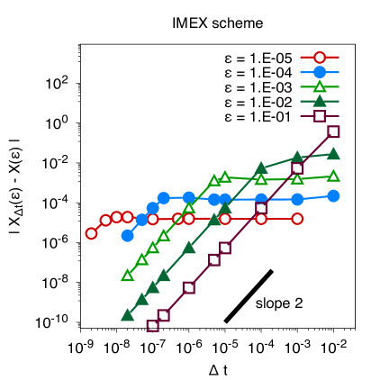
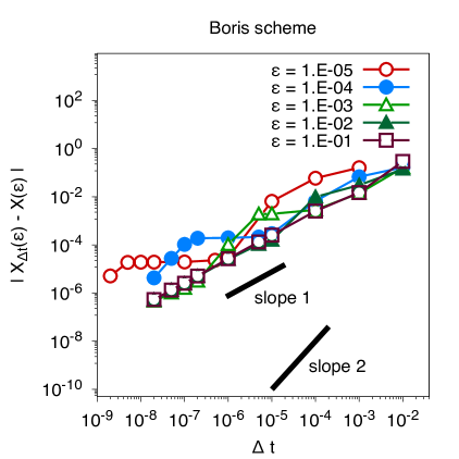
(a)	(b)

Figure 1. Particle motion without electric field. Numerical errors $\|{\mathbf{X}}^{\varepsilon}_{\Delta t}-{\mathbf{X}}^{\varepsilon}\|$ obtained for different $\varepsilon$ with (a) the second order scheme (4.10)-(4.12) and (b) the Boris scheme [2], plotted as functions of $\Delta t$.

The latter observation is expected by design and consistent with Figure 2 where for the same set of simulations we plot errors with respect to the asymptotic system (4.5). This illustrates that, for a fixed $\Delta t$, the scheme (4.10)–(4.12) captures correct first-order dynamics and correct second-order perpendicular drift velocities in the asymptotic $\varepsilon\ll 1$.

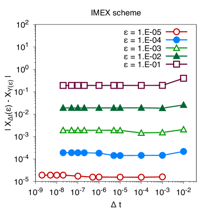
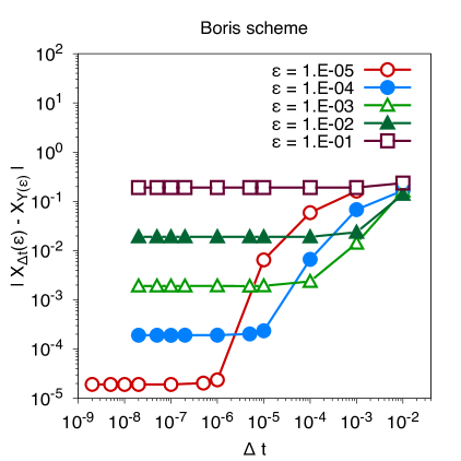
(a)	(b)

Figure 2. Particle motion without electric field. Numerical errors $\|{\mathbf{X}}_{\Delta t}(\varepsilon)-{\mathbf{X}}_{{\mathbf{Y}}(\varepsilon)}\|$, ${\mathbf{X}}_{{\mathbf{Y}}(\varepsilon)}$ being the spatial position built from ${\mathbf{Y}}$, obtained for different $\varepsilon$ with (a) second order scheme (4.10)-(4.12) and (b) the Boris scheme [2], plotted as functions of $\Delta t$.

Finally, in Figures 3 and 4 we show the time evolution of quantities related to slow components $(\mu,v_{\mkern 3.0mu\vphantom{\perp}\vrule depth=0.0pt\mkern 2.0mu\vrule depth=0.0pt\mkern 3.0mu},r,z,{\mathbf{x}})$, obtained with the second-order scheme (4.10)-(4.12) and the Boris scheme, holding fixed both the time step and the stiffness parameter to $\Delta t=0.02$ and $\varepsilon=10^{-2}$, which corresponds to an intermediate regime. Both results are compared with the reference solution computed with a small time step. On the one hand, we observe that the variations of the adiabatic invariant $\mu$ (shown in Figure 3$(a)$ and 4$(a)$) are of order $\varepsilon$ as it is expected but the Boris scheme slightly amplifies these variations whereas our IMEX scheme (4.10)-(4.12) overdamp them. The time evolution of $v_{\mkern 3.0mu\vphantom{\perp}\vrule depth=0.0pt\mkern 2.0mu\vrule depth=0.0pt\mkern 3.0mu}$ given by the IMEX scheme coincides with the one given by the reference solution whereas for large time the Boris scheme exhibits a small phase shift. On the other hand, we also present the projection in the $r$-$z$ plane and $3D$ trajectory in Figures 3 and 4, where ${\mathbf{x}}=(x,y,z)$ denote there Cartesian coordinates. Both results are in good agreement with the ones corresponding to the reference solution. However, again the Boris scheme has some spuriously large oscillations whereas the trajectory obtained with the IMEX scheme is smooth and shows better agreement with spatial positions.

Though we do not show numerical plots, it is worth mentioning that for this test without electric field the kinetic energy is theoretically preserved on the continuous system (4.1) over time. However, the numerical approximation provided by the IMEX scheme (4.10)-(4.12b) does not preserve exactly the discrete kinetic energy and its the fluctuations are of order $10^{-6}$ (and do not increase over time) whereas the fluctuations to the Boris scheme are of order of the round-off error.

(a)	(b)
(c)	(d)

Figure 3. Particle motion without electric field. Time evolution of (a) $\mu$, (b) $v_{\parallel}$, (c) $r$-$z$ projection and (d) 3D trajectory obtained with the second order scheme (4.10)-(4.12) with $\Delta t=2\,10^{-3}$ and $\varepsilon=10^{-2}$.

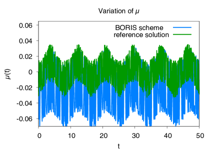
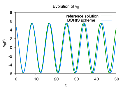
(a)	(b)
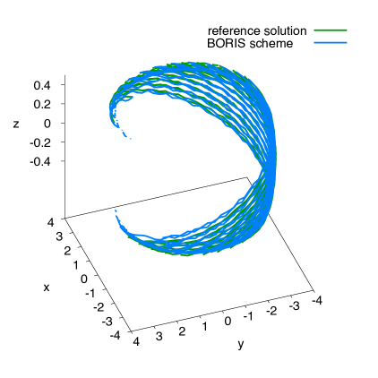
(c)	(d)

Figure 4. Particle motion without electric field. Time evolution of (a) $\mu$, (b) $v_{\parallel}$, (c) $r$-$z$ projection and (d) 3D trajectory obtained with the second order Boris scheme [2] with $\Delta t=2\,10^{-3}$ and $\varepsilon=10^{-2}$.

5.2. Tokamak-like Equilibrium

Now we consider an equilibrium magnetic field in a tokamak-like geometry [5]. Explicitly, a Solov’ev equilibrium solution of the Grad- Shafranov equation for the flux function $\psi$ can be written as

$$\psi(r)=5\,\left(\frac{r^{2}}{2}\,-\,\frac{r^{3}}{3}\right)\,,$$

and, correspondingly, we set

$${\mathbf{B}}:=B_{0}\,\nabla\varphi+\nabla\psi\wedge\nabla\varphi$$

with $B_{0}=50$. Therefore ${\mathbf{B}}=B_{\theta}\,\operatorname{\mathbf{e}}_{\theta}+B_{\varphi}\,\operatorname{\mathbf{e}}_{\varphi}$ with

$$B_{\theta} :=\frac{5\,r\,(1-r)}{R}\,=\,\frac{5\,r\,(1-r)}{R_{0}+r\cos(\theta)}\,, B_{\varphi} :=\frac{B_{0}}{R}\,=\,\frac{B_{0}}{R_{0}+r\cos(\theta)}\,.$$

Additionally, we introduce a compatible electrostatic potential. Our choice is motivated by the fact that, in steady form, the ideal MHD Ohm’s law ${\mathbf{E}}\,+\,{\mathbf{v}}\,\wedge\,{\mathbf{B}}\,=\,0$ requires that ${\mathbf{B}}\cdot{\mathbf{E}}=0$. We set ${\mathbf{E}}=-\nabla\phi$, with electrostatic potential $\phi=-2\,\psi$.

We perform several numerical simulations for various parameters $\varepsilon$ and time steps $\Delta t$. Again, as in Figures 1 and 2, numerical errors show that a better accuracy of our approach based on the combination of augmented formulation (4.1) with IMEX scheme (4.10)-(4.12), allowing in particular the use of a larger time step $\Delta t$ than the ones compatible with the Boris scheme. Since the results are globally the same as the ones shown in the previous section, we do not report them here.

However we complete time evolutions for variables as in focus on the plots of the time evolution of physical quantities as in Figures 3 and 4, with those of the potential and kinetic energy. Explicitly, in Figures 5, 7 and 9, we show plots for energies and $\mu$, whereas in 6, 8 and 10 we show time evolutions of $v_{\mkern 3.0mu\vphantom{\perp}\vrule depth=0.0pt\mkern 2.0mu\vrule depth=0.0pt\mkern 3.0mu}$ and the $r$-$z$ projection of the spatial trajectory. In these experiments we fix $\Delta t=10^{-2}$ whereas the inverse of the amplitude of the magnetic field $\varepsilon$ varies through $\varepsilon=5\,10^{-2}$, $10^{-2}$, $10^{-3}$.

First for $\varepsilon=5\times 10^{-2}$ (and $\Delta t=10^{-2}$), we observe that both numerical outcome (obtained from the IMEX (4.10)-(4.12) and Boris schemes) are in good agreement with the reference solution, even if the IMEX scheme (4.10)-(4.12) has a tendency to overdamp oscillations whereas the Boris scheme seems to slightly overamplify them. This point may be observed for instance on the time evolution of $\mu$ in Figure 5 or in the $r$-$z$ projection of the trajectory in Figure 6, where particles oscillate following a banana trajectory.

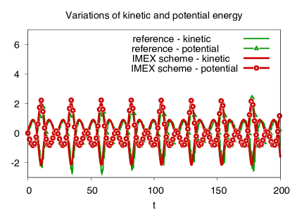
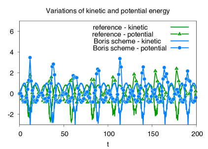
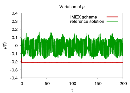
(a)	(b)

Figure 5. Tokamak Equilibrium $\varepsilon=5\,\times\,10^{-2}$. Time variation of kinetic & potential energy and adiabatic invariant $\mu$ obtained with (a) the second order scheme (4.10)-(4.12) and (b) the second order Boris scheme [2], with $\Delta t=10^{-2}$.

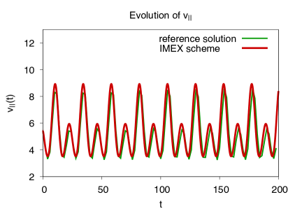
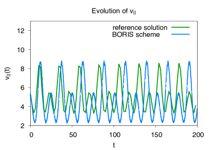
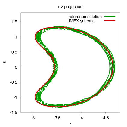
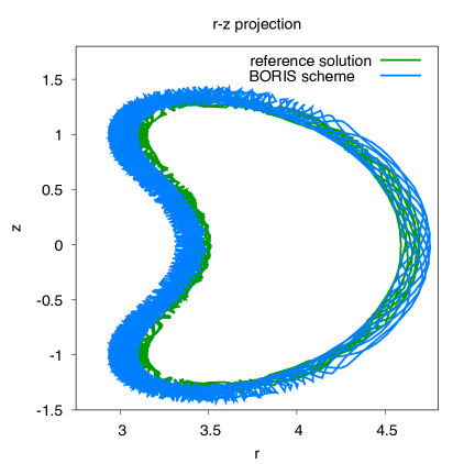
(a)	(b)

Figure 6. Tokamak Equilibrium $\varepsilon=5\,\times\,10^{-2}$. Time evolution of $v_{\parallel}$ and $r$-$z$ projection obtained with (a) the second order scheme (4.10)-(4.12) and (b) the second order Boris scheme [2], with $\Delta t=10^{-3}$.

For a smaller $\varepsilon=10^{-2}$ (and the same time step $\Delta t=10^{-2}$), the trajectory obtained by applying Boris scheme again oscillates with a spuriously larger amplitude. Moreover, for large time ($t\geq 100$) there is a phase shift in time on the evolution of the potential energy and kinetic energy. Let us stress that these spurious oscillations and phase shifts do decrease when taking smaller time steps. However, with the same time step, the IMEX scheme (4.10)-(4.12) is much more stable and gives an accurate approximation of the trajectory even for large times.

Incidentally we point out that on the latter one observes the junction of two bananas in spatial trajectories.

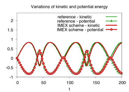
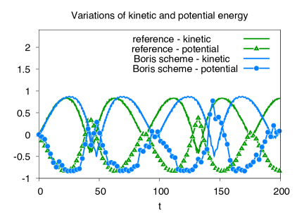
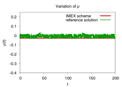
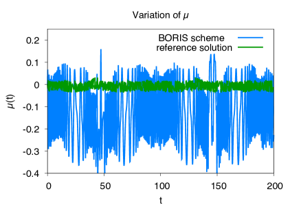
(a)	(b)

Figure 7. Tokamak Equilibrium $\varepsilon=10^{-2}$. Time variation of kinetic & potential energy and adiabatic invariant $\mu$ obtained with (a) the second order scheme (4.10)-(4.12) and (b) the second order Boris scheme [2], with $\Delta t=10^{-2}$.

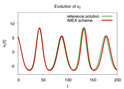
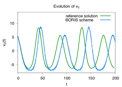
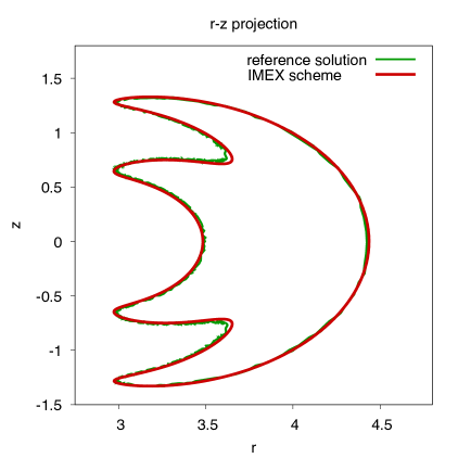
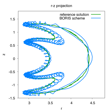
(a)	(b)

Figure 8. Tokamak Equilibrium $\varepsilon=10^{-2}$. Time evolution of $v_{\parallel}$ and $r$-$z$ projection obtained with (a) the second order scheme (4.10)-(4.12) and (b) the second order Boris scheme [2] with $\Delta t=10^{-2}$.

Finally in Figures 9 and (10) we report the numerical results obtained for $\varepsilon=10^{-3}$ (and $\Delta t=10^{-2}$). On the one hand, in this regime, the Boris scheme is still stable but poorly accurate. It produces some oscillations on the different quantities as the potential energy and the adiabatic invariant $\mu$ and the quantity $v_{\mkern 3.0mu\vphantom{\perp}\vrule depth=0.0pt\mkern 2.0mu\vrule depth=0.0pt\mkern 3.0mu}$ very rapidly desynchronizes. On the other hand, the IMEX scheme (4.10)-(4.12) gives smooth and accurate results essentially indistinguishable from the reference ones. It illustrates the robustness of our approach in term of stability and accuracy with respect to $\varepsilon\ll 1$.

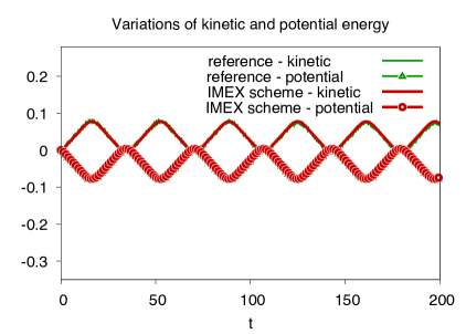
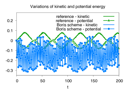
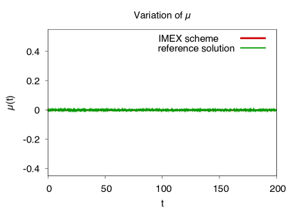
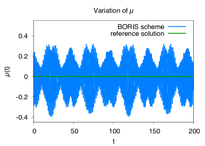
(a)	(b)

Figure 9. Tokamak Equilibrium $\varepsilon=10^{-3}$. Time variation of kinetic & potential energy and adiabatic invariant $\mu$ obtained with (a) the second order scheme (4.10)-(4.12) and (b) the second order Boris scheme [2], with $\Delta t=10^{-2}$.

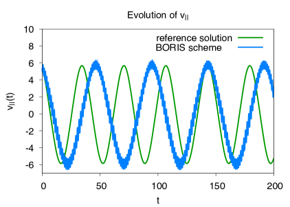
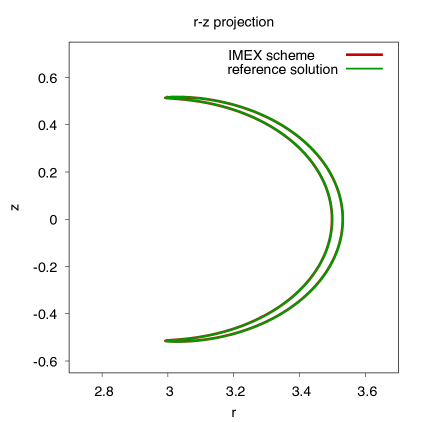
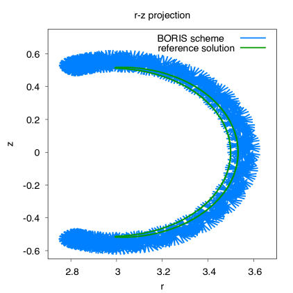
(a)	(b)

Figure 10. Tokamak Equilibrium $\varepsilon=10^{-3}$. Time evolution of $v_{\parallel}$ and $r$-$z$ projection obtained with (a) the second order scheme (4.10)-(4.12) and (b) the second order Boris scheme [2], with $\Delta t=10^{-2}$.

6. Conclusion and perspectives

In the present paper we have proposed a class of semi-implicit time discretization techniques for particle-in cell simulations in torus configurations, mimicking tokamak fusion devices. The main feature of our approach is to guarantee the accuracy and stability on slow scale variables even when the amplitude of the magnetic field becomes large, thus allowing a capture of their correct long-time behavior including cases with non homogeneous magnetic fields and coarse time grids. Even on large time simulations the obtained numerical schemes also provide an acceptable accuracy on physical invariants (total energy for any $\varepsilon$, adiabatic invariant when $\varepsilon\ll 1$) whereas fast scales are automatically filtered when the time step is large compared to $\varepsilon^{2}$.

As a theoretical validation we have proved that the slow part of the approximation converges when $\varepsilon\rightarrow 0$ to the solution of a limiting scheme for the asymptotic evolution, that preserves the initial order of accuracy. Yet a full proof of uniform accuracy and a classification of admissible schemes remains to be carried out.

From a practical point of view, the next natural step would be to consider the coupling with the Poisson equation for the computation of a self-consistent electric field and the consideration of even more realistic geometries.

References

- [1] P. M. Bellan. Fundamentals of plasma physics. Cambridge University Press, 2008.
- [2] J. Boris. Relativistic plasma simulation-optimization. In 4th conference on numerical simulation of plasma, page 3, 1970.
- [3] S. Boscarino, F. Filbet, and G. Russo. High order semi-implicit schemes for time dependent partial differential equations. Journal of Scientific Computing, 68(3):975–1001, 2016.
- [4] J. W. Burby and T. J. Klotz. INVITED: Slow manifold reduction for plasma science. Commun. Nonlinear Sci. Numer. Simul., 89:105289, 62, 2020.
- [5] A. J. Cerfon and J. P. Freidberg. “one size fits all” analytic solutions to the grad–shafranov equation. Physics of Plasmas, 17(3):032502, 2010.
- [6] P. Chartier, N. Crouseilles, M. Lemou, F. Méhats, and X. Zhao. Uniformly accurate methods for Vlasov equations with non-homogeneous strong magnetic field. Math. Comp., 88(320):2697–2736, 2019.
- [7] P. Chartier, N. Crouseilles, M. Lemou, F. Méhats, and X. Zhao. Uniformly accurate methods for three dimensional Vlasov equations under strong magnetic field with varying direction. SIAM J. Sci. Comput., 42(2):B520–B547, 2020.
- [8] G. Chen and L. Chacón. An implicit, conservative and asymptotic-preserving electrostatic particle-in-cell algorithm for arbitrarily magnetized plasmas in uniform magnetic fields. arXiv preprint arXiv:2205.09187, 2022.
- [9] R. Cohen, A. Friedman, D. Grote, and J.-L. Vay. Large-timestep mover for particle simulations of arbitrarily magnetized species. Nuclear Instruments and Methods in Physics Research Section A: Accelerators, Spectrometers, Detectors and Associated Equipment, 577(1):52–57, 2007. Proceedings of the 16th International Symposium on Heavy Ion Inertial Fusion.
- [10] F. Filbet and L. M. Rodrigues. Asymptotically stable particle-in-cell methods for the Vlasov-Poisson system with a strong external magnetic field. SIAM J. Numer. Anal., 54(2):1120–1146, 2016.
- [11] F. Filbet and L. M. Rodrigues. Asymptotically preserving particle-in-cell methods for inhomogeneous strongly magnetized plasmas. SIAM J. Numer. Anal., 55(5):2416–2443, 2017.
- [12] F. Filbet and L. M. Rodrigues. Asymptotics of the three-dimensional Vlasov equation in the large magnetic field limit. J. Éc. polytech. Math., 7:1009–1067, 2020.
- [13] F. Filbet, L. M. Rodrigues, and H. Zakerzadeh. Convergence analysis of asymptotic preserving schemes for strongly magnetized plasmas. Numerische Mathematik, 149(3):549–593, 2021.
- [14] E. Hairer and C. Lubich. Symmetric multistep methods for charged-particle dynamics. SMAI J. Comput. Math., 3:205–218, 2017.
- [15] E. Hairer and C. Lubich. Long-term analysis of a variational integrator for charged-particle dynamics in a strong magnetic field. Numer. Math., 144(3):699–728, 2020.
- [16] E. Hairer, C. Lubich, and Y. Shi. Large-stepsize integrators for charged-particle dynamics over multiple time scales. Numerische Mathematik, pages 1–33, 2022.
- [17] D. Han-Kwan. Contribution à l’étude mathématique des plasmas fortement magnétisés. PhD thesis, Université Pierre et Marie Curie-Paris VI, 2011.
- [18] R. Hazeltine and J. Meiss. Plasma Confinement. Dover Publications, 2003.
- [19] R. Hazeltine and A. Ware. The drift kinetic equation for toroidal plasmas with large mass velocities. Plasma Phys., 20:673–678, 1978.
- [20] M. Herda. Analyse asymptotique et numérique de quelques modèles pour le transport de particules chargées. PhD thesis, Université Claude Bernard Lyon 1, 2017.
- [21] M. Lutz. Étude mathématique et numérique d’un modèle gyrocinétique incluant des effets électromagnétiques pour la simulation d’un plasma de Tokamak. PhD thesis, Université de Strasbourg, 2013.
- [22] K. Miyamoto. Plasma physics and controlled nuclear fusion, volume 38 of Springer Series on Atomic, Optical, and Plasma Physics. Springer-Verlag Berlin-Heidelberg, 2006.
- [23] L. F. Ricketson and L. Chacón. An energy-conserving and asymptotic-preserving charged-particle orbit implicit time integrator for arbitrary electromagnetic fields. Journal of Computational Physics, 418:109639, 2020.
- [24] H. Vu and J. Brackbill. Accurate numerical solution of charged particle motion in a magnetic field. Journal of Computational Physics, 116(2):384–387, 1995.
- [25] B. Wang, X. Wu, and Y. Fang. A two-step symmetric method for charged-particle dynamics in a normal or strong magnetic field. Calcolo, 57(3):Paper No. 29, 21, 2020.
- [26] B. Wang and X. Zhao. Error estimates of some splitting schemes for charged-particle dynamics under strong magnetic field. SIAM Journal on Numerical Analysis, 59(4):2075–2105, 2021.
- [27] S. D. Webb. Symplectic integration of magnetic systems. J. Comput. Phys., 270:570–576, 2014.
Francis Filbet
Université de Toulouse III
UMR5219, IMT,
118, route de Narbonne
F-31062 Toulouse cedex, FRANCE
e-mail: francis.filbet@math.univ-toulouse.fr
Luis Miguel Rodrigues
Univ Rennes & IUF,
CNRS, IRMAR - UMR 6625,
F-35000 Rennes, FRANCE
e-mail: luis-miguel.rodrigues@univ-rennes1.fr