Quantization for decentralized learning
under subspace constraints

Abstract

In this paper, we consider decentralized optimization problems where agents have individual cost functions to minimize subject to subspace constraints that require the minimizers across the network to lie in low-dimensional subspaces. This constrained formulation includes consensus or single-task optimization as special cases, and allows for more general task relatedness models such as multitask smoothness and coupled optimization. In order to cope with communication constraints, we propose and study an adaptive decentralized strategy where the agents employ differential randomized quantizers to compress their estimates before communicating with their neighbors. The analysis shows that, under some general conditions on the quantization noise, and for sufficiently small step-sizes $\mu$, the strategy is stable both in terms of mean-square error and average bit rate: by reducing $\mu$, it is possible to keep the estimation errors small (on the order of $\mu$) without increasing indefinitely the bit rate as $\mu\rightarrow 0$ when variable-rate quantizers are used. Simulations illustrate the theoretical findings and the effectiveness of the proposed approach, revealing that decentralized learning is achievable at the expense of only a few bits.

I Introduction

Mobile phones, wearable devices, and autonomous vehicles are examples of modern distributed networks generating massive amounts of data each day. Due to the growing computational power in these devices and the increasing size of the datasets, coupled with concerns over privacy, federated and decentralized training of statistical models have become desirable and often necessary [2, 3, 4, 5, 6, 7, 8, 9, 10, 11]. In these approaches, each participating device (which is referred to as agent or node) has a local training dataset, which is never uploaded to the server. The training data is kept locally on the users’ devices, which also serve as computational agents acting on the local data in order to update global models of interest. In applications where communication with a server becomes a bottleneck, decentralized topologies (where agents only communicate with their neighbors) are attractive alternatives to federated topologies (where a server connects with all remote devices). Compared to federated approaches[2, 3, 4, 5, 6, 7], decentralized implementations reduce the high communication cost on the central server since, in this case, the model updates are exchanged locally between agents without relying on a central coordinator [12, 8, 9, 10, 11].

In practice, there are several issues that arise in the implementations of decentralized algorithms due to the use of a communication network. For instance, in modern distributed networks comprising a massive number of devices, e.g., thousands of participating smartphones, communication can be slower than local computation by many orders of magnitude (due to limited resources such as energy and bandwidth). Designers are typically limited by an upload bandwidth of 1MB/s or less [2]. While there have been significant works in the literature on solving optimization and inference problems in a decentralized manner [13, 14, 15, 8, 9, 10, 11, 16, 17, 18, 19, 20, 21, 22, 23, 24, 25, 26, 27, 28, 29, 30, 31, 32, 33, 34, 12, 35, 36, 37, 38, 39], with some exceptions [12, 27, 32, 33, 30, 31, 28, 29, 34, 39, 37, 35, 36, 38], the large majority of these works is not tailored to the specific challenge of limited communication capabilities. Moreover, the existing works on decentralized approaches are often designed only to solve consensus-based optimization problems. And many of these existing approaches rely mainly on quantization rules that assume that some quantities are represented with very high precision and neglect the associated quantization error in the theoretical analyses.

In this work, we do not make any assumptions about the high-precision representation of specific variables. Moreover, we consider quantization for decentralized learning under subspace constraints by studying the effects of quantization on the performance of the following decentralized stochastic gradient approach from [24, 25]:

$$\boldsymbol{\psi}_{k,i} =\boldsymbol{w}_{k,i-1}-\mu\widehat{\nabla_{w_{k}}J_{k}}(\boldsymbol{w}_{k,i-1})$$ (1a)

$$\boldsymbol{w}_{k,i} =\sum_{\ell\in\mathcal{N}_{k}}A_{k\ell}\boldsymbol{\psi}_{\ell,i}$$ (1b)

where $\mu>0$ is a small step-size parameter, $\mathcal{N}_{k}$ is the neighborhood set of agent $k$ (i.e., the set of nodes connected to agent $k$ by a communication link or edge, including node $k$ itself), $A_{k\ell}$ is an $M_{k}\times M_{\ell}$ matrix associated with link $(k,\ell)$, $w_{k}\in\mathbb{R}^{M_{k}}$ is the parameter vector at agent $k$, and $J_{k}(w_{k}):\mathbb{R}^{M_{k}}\rightarrow\mathbb{R}$ is a differentiable convex cost associated with agent $k$. This cost is usually expressed as the expectation of some loss function $L_{k}(\cdot)$ and written as $J_{k}(w_{k})=\mathbb{E}\,L_{k}(w_{k};\boldsymbol{y}_{k})$, where $\boldsymbol{y}_{k}$ denotes the random data at agent $k$ (throughout the paper, random quantities are denoted in boldface). The expectation is computed relative to the distribution of the local data. In the stochastic-optimization framework, the statistical distribution of the data $\boldsymbol{y}_{k}$ is usually unknown and, hence, the risks $J_{k}(\cdot)$ and their gradients $\nabla_{w_{k}}J_{k}(\cdot)$ are unknown. In this case, and instead of using the true gradient, it is common to use approximate gradient vectors such as $\widehat{\nabla_{w_{k}}J_{k}}(w_{k})=\nabla_{w_{k}}L_{k}(w_{k};\boldsymbol{y}_{k,i})$, where $\boldsymbol{y}_{k,i}$ represents the data realization observed at iteration $i$ [8]. We note that a unique feature of algorithm (1) is the utilization of matrix valued combination weights, as opposed to scalar weighting as is commonly employed in conventional consensus and diffusion optimization [13, 8]. As explained in the next paragraph, this generalization allows the network to solve a broader class of multitask optimization problems beyond classical consensus. Multitask learning is suitable for network applications where regional differences in the data require more complex models and more flexible algorithms than single-task or consensus implementations. In multitask networks, agents generally need to estimate and track multiple distinct, though related, objectives. For instance, in distributed power state estimation problems, the local state vectors at neighboring control centers may overlap partially since the areas in a power system are interconnected [19]. Likewise, in weather forecasting applications, regional differences in the collected data distributions require agents to exploit the correlation profile in the data for enhanced decision rules [21]. Other multitask network applications include distributed minimum-cost flow [17, 18], distributed active noise control [16], and distributed sub-optimal beamforming [24].

Let $N$ denote the total number of agents and let ${\scriptstyle\mathcal{W}}=\text{col}\{w_{1},\ldots,w_{N}\}$ denote the $M-$th dimensional vector (where $M=\sum_{k=1}^{N}M_{k}$) collecting the parameter vectors from across the network. Let $\mathcal{A}$ denote the $N\times N$ block matrix whose $(k,\ell)$-th block is $A_{k\ell}$ if $\ell\in\mathcal{N}_{k}$ and $0$ otherwise. It was shown in [24, Theorem 1] that, for sufficiently small $\mu$ and for a combination matrix $\mathcal{A}$ satisfying:

$$\mathcal{A}\,\mathcal{U}=\mathcal{U},\quad\mathcal{U}^{\top}\mathcal{A}=\mathcal{U}^{\top},~{}~{}\text{and~{} }\rho(\mathcal{A}-\mathcal{P}_{{\scriptscriptstyle\mathcal{U}}})<1,$$ (2)

where $\rho(\cdot)$ denotes the spectral radius of its matrix argument, $\mathcal{U}$ is any given $M\times P$ full-column rank matrix (with $P\ll M$) that is assumed to be semi-unitary, i.e., its columns are orthonormal ($\mathcal{U}^{\top}\mathcal{U}=I_{P}$), and $\mathcal{P}_{{\scriptscriptstyle\mathcal{U}}}=\mathcal{U}\mathcal{U}^{\top}$ is the orthogonal projection matrix onto $\text{Range}(\mathcal{U})$, strategy (1) will converge in the mean-square-error sense to the solution of the following subspace constrained optimization problem:

$$\begin{split}{\scriptstyle\mathcal{W}}^{o}=&\arg\min_{{\scriptscriptstyle\mathcal{W}}}~{}J^{\text{glob}}({\scriptstyle\mathcal{W}})\triangleq\sum_{k=1}^{N}J_{k}(w_{k})\\ &\operatorname*{subject~{}to}~{}{\scriptstyle\mathcal{W}}\in\text{Range}(\mathcal{U}).\end{split}$$ (3)

In particular, it was shown that $\limsup_{i\rightarrow\infty}\mathbb{E}\|w^{o}_{k}-\boldsymbol{w}_{k,i}\|^{2}=O(\mu)$ for all $k$, where $w^{o}_{k}$ is the $k$-th $M_{k}\times 1$ subvector of ${\scriptstyle\mathcal{W}}^{o}$. As explained in [11], [26], [24, Sec. II], by properly selecting $\mathcal{U}$ and $\mathcal{A}$, strategy (1) can be employed to solve different decentralized optimization problems such as (i) consensus or single-task optimization (where, as explained in Remark 1 further ahead, the agents’ objective is to reach a consensus on the minimizer of the aggregate cost $\sum_{k=1}^{N}J_{k}(w)$) [13, 8, 9, 10], (ii) decentralized coupled optimization (where the parameter vectors to be estimated at neighboring agents are partially overlapping) [16, 17, 19, 20, 22], and (iii) multitask inference under smoothness (where the network parameter vector ${\scriptstyle\mathcal{W}}$ to be estimated is smooth w.r.t. the underlying network topology) [24, 23]. For instance, while projecting onto the space spanned by the vector of all ones allows to enforce consensus across the network (see Remark 1), graph smoothness can in general be promoted by projecting onto the space spanned by the eigenvectors of the graph Lapacian corresponding to small eigenvalues (see the simulation section VI for an illustration). Besides being capable of solving single-task or consensus-based optimization problems, the constrained formulation (3) and its decentralized solution (1) are general enough to apply to a wide variety of network applications, including those listed in the previous paragraph.

The first step (1a) in algorithm (1) is the self-learning step corresponding to the stochastic gradient descent step on the individual cost $J_{k}(\cdot)$. This step is followed by the social learning step (1b) where agent $k$ receives the intermediate estimates $\{\boldsymbol{\psi}_{\ell,i}\}$ from its neighbors $\ell\in\mathcal{N}_{k}$ and combines them through $\{A_{k\ell}\}$ to form $\boldsymbol{w}_{k,i}$, which corresponds to the estimate of $w^{o}_{k}$ at agent $k$ and iteration $i$. To alleviate the communication bottleneck resulting from the exchange of the intermediate estimates among agents over many iterations, quantized communication must be considered. In this paper, we study the effect of quantization on the convergence properties of the decentralized learning approach (1). First, we describe in Sec. II the class of randomized quantizers considered in this study. Then, we propose in Sec. III a differential randomized quantization strategy for solving problem (3) – see (28) further ahead. Compared with the unquantized version (1), the new approach consists of three steps where a quantization step is added. Interestingly, instead of exchanging compressed versions of the intermediate estimates $\{\boldsymbol{\psi}_{\ell,i}\}$, and due to differential quantization, the agents in the proposed solution exchange compressed versions of the differences between subsequent iterates (which tend to have a reduced range when compared to the intermediate estimates). At the receiver side, prediction rules are implemented in order to reconstruct the intermediate estimates. This step leads to a new set of intermediate estimates $\{\boldsymbol{\phi}_{\ell,i}\}$ which are then: (i) stored at the receiver in order to be used as predictors in the next iteration, and (ii) combined according to a modified version of the combination step. In the modified version, a mixing parameter $\gamma$ is introduced in order to control the mixing speed of the algorithm. This allows to control the network stability in situations where quantization can lead to network instability. We establish in Sec. IV that, under some general conditions on the quantization noise and mixing parameter, and for sufficiently small step-sizes $\mu$, the decentralized quantized approach is stable in the mean-square error sense. In addition to investigating the mean-square-error stability, we characterize the steady-state average bit rate of the proposed approach when variable-rate quantizers are used. The analysis shows that, by properly designing the quantization operators, the iterates generated by the quantized decentralized adaptive implementation lead to small estimation errors on the order of $\mu$ (as it happens in the ideal case without quantization), while concurrently guaranteeing a bounded average bit rate as $\mu\rightarrow 0$. While there exist several useful works in the literature that study decentralized learning approaches in the presence of differential quantization [33, 32, 34, 12, 38, 31, 40, 37, 35, 36, 39], these works investigate standard consensus or single-task optimization, and do not consider the subspace constrained formulation (3) or multitask variants. Moreover, with some exceptions that consider deterministic optimization [31, 40, 39], the analyses conducted in these works assume that some quantities (e.g., the norm or some components of the vector to be quantized) are represented with very high precision (e.g., machine precision) and the associated quantization error is neglected. On the other hand, the analysis in the current work is not limited to standard consensus optimization and does not assume a machine precision representation of some quantities – a detailed discussion of related work is provided in Sec. III-B.

Notation: All vectors are column vectors. Random quantities are denoted in boldface. Matrices are denoted in uppercase letters while vectors and scalars are denoted in lower-case letters. The symbol $(\cdot)^{\top}$ denotes matrix transposition. The operator $\text{col}\{\cdot\}$ stacks the column vector entries on top of each other. The operator $\text{diag}\{\cdot\}$ forms a matrix from block arguments by placing each block immediately below and to the right of its predecessor. The symbol $\otimes$ denotes the Kronecker product. The $M\times M$ identity matrix is denoted by $I_{M}$. The abbreviation “w.p.” is used for “with probability”. The Gaussian distribution with mean $m$ and covariance $C$ is denoted by ${\mathcal{N}}(m,C)$. The notation $\alpha=O(\mu)$ signifies that there exist two positive constants $c$ and $\mu_{0}$ such that $|\alpha|\leq c\mu$ for all $\mu\leq\mu_{0}$. A vector of all zeros is denoted by 0. For tables, the header is not counted as a row (i.e., “first row” means the first row after the header).

II Randomized quantizers

In this paper, we study decentralized learning under subspace constraints in the presence of quantized communications. Randomized quantizers $\boldsymbol{\cal{Q}}(\cdot)$ will be employed instead of deterministic quantizers. As explained in [33], deterministic quantizers can lead to severe estimation biases in inference problems. To overcome this issue, randomized quantizers $\boldsymbol{\cal{Q}}(\cdot)$ are commonly used to compensate for the bias (on average, over time) [12, 32, 33, 34, 31, 38]. This section is devoted to describing the class of randomized quantizers considered throughout the study.

For any deterministic input $x\in\mathbb{R}^{L}$ with $L$ representing a generic vector length, the randomized quantizer $\boldsymbol{\cal{Q}}(\cdot)$ is characterized in terms of a probability $\mathbb{P}[\boldsymbol{\cal{Q}}(x)=y]$ for any $y$ belonging to the set of output levels of the quantizer. We consider randomized quantizers $\boldsymbol{\cal{Q}}(\cdot)$ satisfying the following general property, which as explained in the sequel, relaxes the condition on the mean-square error from [32, 12, 5, 34, 33, 38].

Property 1.

(Unbiasedness and variance bound). The randomized quantizer $\boldsymbol{\cal{Q}}(\cdot)$ satisfies the following two conditions:

$$\mathbb{E}[x-\boldsymbol{\cal{Q}}(x)] =0,$$ (4)

$${\mathbb{E}\|x-\boldsymbol{\cal{Q}}(x)\|^{2}} \leq\beta^{2}_{q}\|x\|^{2}+\sigma^{2}_{q},$$ (5)

for some $\beta^{2}_{q}\geq 0$ and $\sigma^{2}_{q}\geq 0$, and where the expectations are evaluated w.r.t. the randomness of $\boldsymbol{\cal{Q}}(\cdot)$. When the quantizers are applied to a random input $\boldsymbol{x}$, conditions (4) and (5) become:

$$\mathbb{E}[\boldsymbol{x}-\boldsymbol{\cal{Q}}(\boldsymbol{x})|\boldsymbol{x}] =0,$$ (6)

$${\mathbb{E}[\|\boldsymbol{x}-\boldsymbol{\cal{Q}}(\boldsymbol{x})\|^{2}|\boldsymbol{x}]} \leq\beta^{2}_{q}\|\boldsymbol{x}\|^{2}+\sigma^{2}_{q}.$$ (7)

∎

Property 1 is satisfied by many randomized quantization operators of interest in decentralized learning. Table I further ahead lists some typical choices (a detailed comparison of the various schemes will be provided in Sec. III-B). Many existing works focus on studying decentralized learning approaches in the presence of randomized quantizers that satisfy the unbiasedness condition (4) and the variance bound (5) with the absolute noise term $\sigma^{2}_{q}=0$ [32, 12, 5, 34, 33, 38]. In contrast, the analysis in the current work is general and does not require $\sigma^{2}_{q}$ to be zero. As we will explain in Sec. III-B, neglecting the effect of $\sigma^{2}_{q}$ requires that some quantities (e.g., the norm of the vector to be quantized) are represented with no quantization error, in practice at the machine precision. In the following, we describe a useful framework for designing randomized quantizers that do not require high-precision quantization of specific variables.

II-A Uniform and non-uniform randomized quantizers

II-A1 Quantizers’ design

Let $x\in\mathbb{R}^{L}$ denote the input vector to be quantized with $x_{j}$ representing the $j$-th element of $x$. We consider a general quantization rule $\boldsymbol{\cal{Q}}:\mathbb{R}^{L}\rightarrow\mathbb{R}^{L}$ of the following form – see Fig. 1 for an illustration:

$$[\boldsymbol{\cal{Q}}(x)]_{j}=y_{\boldsymbol{n}(x_{j})},$$ (8)

where $[\boldsymbol{\cal{Q}}(x)]_{j}$ denotes the $j$-th element of $\boldsymbol{\cal{Q}}(x)$ and $y_{\boldsymbol{n}(x_{j})}$ is the quantization output level (defined further ahead in (11)) associated with a realization of the random index $\boldsymbol{n}(x_{j})\in\{m,m+1\}$. The probabilistic rule to choose $\boldsymbol{n}(x_{j})$ is as follows:

$$\boldsymbol{n}(x_{j})=\left\{\begin{array}[]{ll}m,&\text{w.p. }\frac{y_{m+1}-x_{j}}{y_{m+1}-y_{m}},\\ m+1,&\text{w.p. }\frac{x_{j}-y_{m}}{y_{m+1}-y_{m}}.\end{array}\right.$$ (9)

Regarding the integer $m$ in (9), and motivated by the so-called companding procedure [41], which can be conveniently described in terms of a non-linear function and its inverse, it is found according to (the dependence of $m$ on $x_{j}$ is left implicit in (9) for ease of notation):

$$m=\lfloor g(x_{j})\rfloor,$$ (10)

where $\lfloor\cdot\rfloor$ denotes the floor function and $g:\mathbb{R}\rightarrow\mathbb{R}$ is some strictly increasing continuous function. Given the inverse function $h=g^{-1}$, the output level associated with an index $m$ is defined by:

$$y_{m}=h(m).$$ (11)

By evaluating the expected value of $[\boldsymbol{\cal{Q}}(x)]_{j}$ w.r.t. the quantizer randomness, we obtain:

$$\mathbb{E}[\boldsymbol{\cal{Q}}(x)]_{j}\overset{\eqref{eq: non-uniform quantization},\eqref{eq: random index n}}{=}\left(y_{m}\frac{y_{m+1}-x_{j}}{y_{m+1}-y_{m}}+y_{m+1}\frac{x_{j}-y_{m}}{y_{m+1}-y_{m}}\right)=x_{j},$$ (12)

which establishes the unbiasedness condition (4) in Property 1.

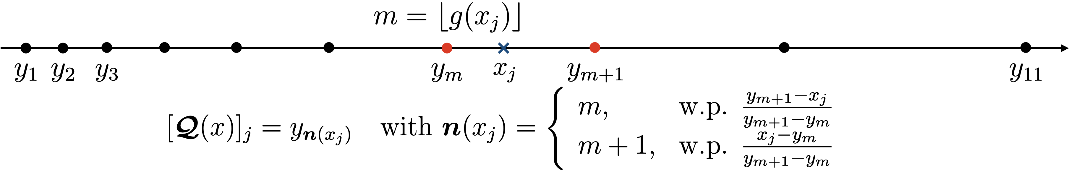
Figure 1: An illustration of the non-uniform randomized quantization scheme defined by (8)–(11). The real axis partition is constructed by choosing the functions $g(\cdot)$ and $h(\cdot)$ according to (15) with $a=4.17$ and $b=10$.

Example 1. (Randomized uniform or dithered quantizer [42, 40]). By choosing:

$$g(t)=\frac{t}{\Delta},\qquad h(t)=\Delta\cdot t,$$ (13)

we obtain the uniform quantizer described in Table I (second row) with a quantization step $\Delta>0$. Condition (5) (with $\beta^{2}_{q}=0$ and $\sigma^{2}_{q}=\frac{L\Delta^{2}}{4}$) can be established by letting $p=\frac{y_{m+1}-x_{j}}{y_{m+1}-y_{m}}$ and by evaluating the variance:

$$\mathbb{E}(x_{j}-[\boldsymbol{\cal{Q}}(x)]_{j})^{2} =(x_{j}-y_{m})^{2}p+(x_{j}-y_{m+1})^{2}(1-p)$$

$$=\Delta^{2}p(1-p)\leq\frac{\Delta^{2}}{4},$$ (14)

where we replaced $y_{m+1}-y_{m}$ by ${\Delta}$ and we used the fact that $p(1-p)\leq\frac{1}{4}$ for $p\in[0,1]$.$\hfill\blacksquare$

TABLE I: Examples of quantizers $\boldsymbol{\cal{Q}}:\mathbb{R}^{L}\rightarrow\mathbb{R}^{L}$ satisfying Property 1. For each scheme, we report the quantization rule, the parameters $\beta_{q}^{2}$ and $\sigma^{2}_{q}$ in (5), and the bit-budget. $B_{\text{HP}}$ denotes the number of bits required to encode a scalar with high precision (Typical values for $B_{\text{HP}}$ are $32$ or $64$).

Quantizer name	Rule	$\beta^{2}_{q}$	$\sigma^{2}_{q}$	Bit-budget
No compression [24]	$\boldsymbol{\cal{Q}}(x)=x$	$0$	$0$	$LB_{\text{HP}}$
Probabilistic uniform	$\left[\boldsymbol{\cal{Q}}(x)\right]_{j}=\Delta\cdot\boldsymbol{n}(x_{j})$	0	$L\frac{\Delta^{2}}{4}$	$\boldsymbol{r}(x)$ defined in (27)
or dithered	$\boldsymbol{n}(x_{j})=\left\{\begin{array}[]{ll}m,&\text{w.p. }\frac{(m+1)\Delta-x_{j}}{\Delta},\\ m+1,&\text{w.p. }\frac{x_{j}-m\Delta}{\Delta},\end{array}\right.\qquad m=\left\lfloor\frac{x_{j}}{\Delta}\right\rfloor$
quantizer [42, 40]	$\Delta$ is the quantization step
Probabilistic ANQ [31]	$\left[\boldsymbol{\cal{Q}}(x)\right]_{j}=y_{\boldsymbol{n}(x_{j})}$	$2\omega^{2}$	$2L\eta^{2}$	$\boldsymbol{r}(x)$ defined in (27)
	$\boldsymbol{n}(x_{j})=\left\{\begin{array}[]{ll}m,&\text{w.p. }\frac{y_{m+1}-x_{j}}{y_{m+1}-y_{m}},\\ m+1,&\text{w.p. }\frac{x_{j}-y_{m}}{y_{m+1}-y_{m}},\end{array}\right.\quad m=\left\lfloor\text{sign}(x_{j})\frac{\ln\left(1+\frac{\omega}{\eta}|x_{j}|\right)}{2\ln\left(\omega+\sqrt{1+\omega^{2}}\right)}\right\rfloor$
	$y_{m}=\text{sign}(m)\frac{\eta}{\omega}\left[\left(\omega+\sqrt{1+\omega^{2}}\right)^{2|m|}-1\right]$
	$\omega$ and $\eta$ are two non-negative design parameters
Rand-$c$ [34]	$\left[\boldsymbol{\cal{Q}}(x)\right]_{j}=\left\{\begin{array}[]{ll}\frac{L}{c}\cdot x_{j},&\text{if }x_{j}\in\Omega_{c}\\ 0,&\text{otherwise }\end{array}\right.$ $\qquad\qquad(c\in\{1,\ldots,L\})$	$\left(\frac{L}{c}-1\right)$	$0$	$cB_{\text{HP}}+c\lceil\log_{2}(L)\rceil$
	$\Omega_{c}$ is a set of $c$ randomly selected coordinates
Randomized Gossip [12]	$\boldsymbol{\cal{Q}}(x)=\left\{\begin{array}[]{ll}\frac{x}{q},&\text{w.p. }q\\ 0,&\text{w.p. }1-q\end{array}\right.$ $\qquad\qquad(q\in(0,1])$	$\left(\frac{1}{q}-1\right)$	$0$	$(LB_{\text{HP}})q\qquad$ (on average)
Gradient sparsifier [40]	$\left[\boldsymbol{\cal{Q}}(x)\right]_{j}=\left\{\begin{array}[]{ll}\frac{x_{j}}{q_{j}},&\text{w.p. }q_{j}\\ 0,&\text{w.p. }1-q_{j}\end{array}\right.$	$\frac{1}{\min\limits_{j}\{q_{j}\}}-1$	$0$	$\sum\limits_{j=1}^{L}q_{j}(B_{\text{HP}}+\lceil\log_{2}(L)\rceil)$
	$q_{j}$ is the probability that coordinate $j$ is selected			(on average)
QSGD [5]	$\left[\boldsymbol{\cal{Q}}(x)\right]_{j}=\|x\|\cdot\text{sign}(x_{j})\cdot\frac{\boldsymbol{n}(x_{j},x)}{s}$	$\min\left(\frac{L}{s^{2}},\frac{\sqrt{L}}{s}\right)$	$0$	$B_{\text{HP}}+L+L\lceil\log_{2}(s)\rceil$
	$\boldsymbol{n}(x_{j},x)=\left\{\begin{array}[]{ll}m,&\text{w.p. }(m+1)-\frac{|x_{j}|}{\|x\|}s,\\ m+1,&\text{w.p. }\frac{|x_{j}|}{\|x\|}s-m,\end{array}\right.\qquad m=\left\lfloor s\frac{|x_{j}|}{\|x\|}\right\rfloor$
	$s$ is the number of quantization levels

Example 2. (Randomized logarithmic companding). For non-uniform quantizers, one popular choice is logarithmic companding, which corresponds to the following direct and inverse non-linear functions [41]:

$$g(t)=\text{sign}(t)\,a\ln(1+b|t|),\quad{h(t)=\text{sign}(t)\frac{1}{b}\left(e^{\frac{|t|}{a}}-1\right)},$$ (15)

with $a>0$ and $b>0$. Two useful results were established in [31] regarding this choice. First, it was shown that, by setting the constants $a$ and $b$ according to:

$$a=\frac{1}{2\ln(\omega+\sqrt{1+\omega^{2}})},\qquad b=\frac{\omega}{\eta},$$ (16)

we obtain the following bound on the variance:

$${\mathbb{E}\|x-\boldsymbol{\cal{Q}}(x)\|^{2}\leq\left(\omega\|x\|+\sqrt{L}\eta\right)^{2}}.$$ (17)

The choice (16) gives the probabilistic ANQ rule reported in Table I (third row) with the non-linear functions given by:

$$\left\{\begin{array}[]{l}g(t)=\text{sign}(t)\,\frac{\ln\left(1+\frac{\omega}{\eta}|t|\right)}{2\ln(\omega+\sqrt{1+\omega^{2}})},\\ h(t)=\text{sign}(t)\frac{\eta}{\omega}\left[(\omega+\sqrt{1+\omega^{2}})^{2|t|}-1\right].\end{array}\right.$$ (18)

Second, it was shown in [31] that, for a fixed number of output levels, the choice in (16) maximizes the range of the input variable while still satisfying the error bound (17). This property justifies the efficiency of the choice (16) in terms of quantization bit rate.

Now, by taking the limit of $g(t)$ in (18) as $\omega\rightarrow 0$ and by applying l’Hôpital’s rule, we get:

$$\lim_{\omega\rightarrow 0}g(t)=\text{sign}(t)\frac{|t|}{2\eta}=\frac{t}{2\eta},$$ (19)

from which we conclude that the setting where $\omega=0$ allows us to recover the uniform quantizer (13) of Example 1.

Finally, we can relate the quantizer parameters $\omega$ and $\eta$ to the constants $\beta^{2}_{q}$ and $\sigma^{2}_{q}$ appearing in (5). In fact, by applying Jensen’s inequality to (17), we can see that the bound in (5) is satisfied with:

$$\beta^{2}_{q}=\frac{\omega^{2}}{\alpha},\qquad\sigma^{2}_{q}=\frac{L\eta^{2}}{1-\alpha},\qquad\text{for any }\alpha\in(0,1).$$ (20)

$\hfill\blacksquare$

II-A2 Variable-rate coding scheme and bit budget [31]

Note that the quantization rule (8)–(11) maps a continuous variable to some integer by partitioning the real line into an infinite number of intervals. Thus, a fixed-rate quantizer (i.e., a quantizer that uses the same number of bits for any input) cannot represent all possible intervals of the partition. On the other hand, assuming a finite support for the quantizer input would require some boundedness assumptions (e.g., on the iterates, on the gradient) that are usually violated in stochastic optimization theory [43]. By following a standard approach in coding theory, we shall instead investigate the use of variable-rate quantizers which are able to adapt the bit rate based on the quantizer input, e.g., assigning more bits to larger inputs and less bits to smaller ones. In this work, we illustrate the main concepts by focusing on the variable-rate coding scheme proposed in [31] and described in the following. This rule has the advantage of not requiring any knowledge about the distribution of the variables to be quantized. This is particularly relevant since such knowledge is typically unavailable in learning applications.

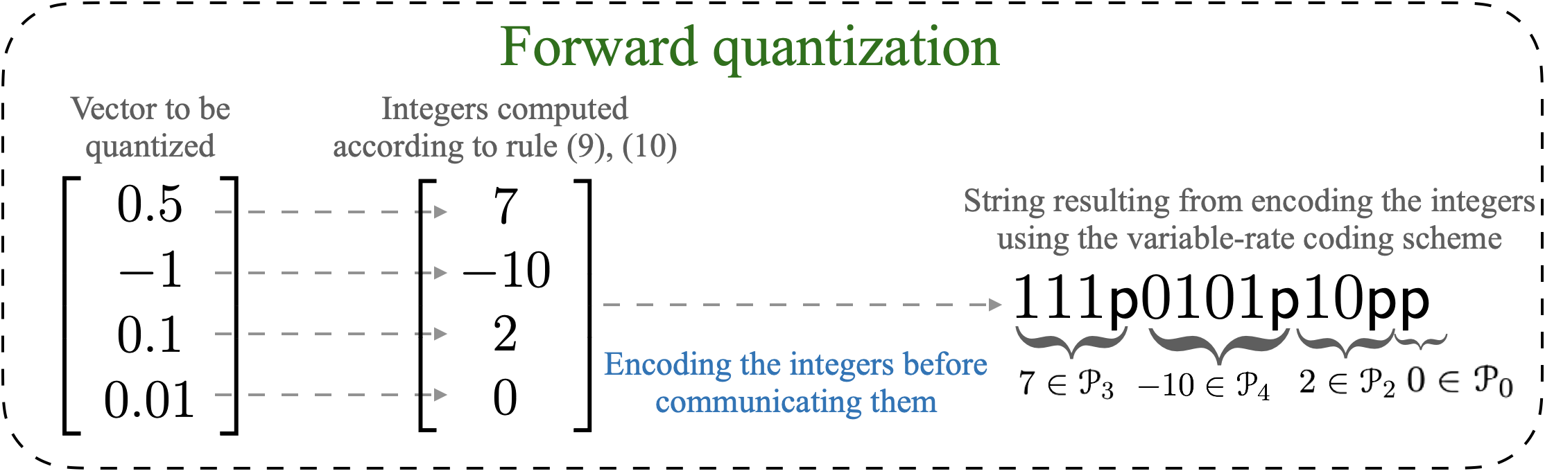
Figure 2: Illustration of the variable-rate coding scheme. The non-uniform randomized quantization scheme defined by (8)–(11) is used. The function $g(\cdot)$ is chosen according to (15) with $a=4.17$ and $b=10$. In this example, the codeword associated with the $j$-th element of the ordered set $\mathscr{P}_{b}$ is given by the $b$-bit binary representation of the integer $j-1$. For instance, the codewords associated with the first element in $\mathscr{P}_{3}$ (which is $-7$ according to (21)) and the sixth element in $\mathscr{P}_{4}$ (which is $-10$ according to (22)) are $000$ and $0101$, respectively. Subsequent integers are separated by a parsing symbol $\mathsf{p}$.

Consider the following partition of the set of integers $\mathbb{Z}$:

$$\begin{split}\mathscr{P}_{0}=\{0\},&\quad\mathscr{P}_{1}=\{-1,1\},\quad\mathscr{P}_{2}=\{-3,-2,2,3\},\\ &\mathscr{P}_{3}=\{-7,-6,-5,-4,4,5,6,7\},\quad\ldots\end{split}$$ (21)

which can be written more compactly as:

$$\mathscr{P}_{b}=\left\{\begin{array}[]{ll}\{0\},&\text{if }b=0\\ \{-1,1\},&\text{if }b=1\\ \{-2^{b}+1,\ldots,-2^{b-1},2^{b-1},\ldots,2^{b}-1\},&\text{if }b\geq 2.\\ \end{array}\right.$$ (22)

Note that the ensemble of sets $\{\mathscr{P}_{b}|b=0,1,2,\ldots\}$ forms a partition of $\mathbb{Z}$ where each set $\mathscr{P}_{b}$ has cardinality equal to $2^{b}$. Thus, an integer $n\in\mathscr{P}_{b}$ can be represented with a string of $b$ bits. Accordingly, from (22), the number of bits to represent an integer $n\in\mathbb{Z}$ can be determined according to:

$$b=\lceil\log_{2}(|n|+1)\rceil,$$ (23)

where $\lceil\cdot\rceil$ denotes the ceiling function. When the rule (8)–(11) is implemented to quantize an input vector $x\in\mathbb{R}^{L}$, a sequence of integers will be generated according (8) and (9). These integers must be encoded before being transmitted over the communication links–see Fig. 2 for an illustration. Thus, we need to encode sequences of integers $n_{1},n_{2},\ldots,$ with different integers belonging in general to different partitions $\mathscr{P}_{b}$. At the receiver side, and since the transmitted integers are unknown, the decoder does not know the number of bits used for each integer. In order to solve this issue, the work [31] proposes to consider an overall encoder alphabet $\mathscr{S}$ made of two binary digits plus a parsing symbol $\mathsf{p}$, namely, $\mathscr{S}=\{0,1\}\cup\{\mathsf{p}\}$. In this way, we can encode a sequence of integers $n_{1},n_{2},\ldots,$ by first encoding each of the individual integers using a number of bits determined by the corresponding partition, and then using the parsing symbol to separate subsequent integers. For example, a string of the form (see also Fig. 2):

$$\underbrace{\mathsf{111\mathsf{p}}}_{n_{1}}\underbrace{0101\mathsf{p}}_{n_{2}}\underbrace{10\mathsf{p}}_{n_{3}}\underbrace{\mathsf{p}}_{n_{4}}$$ (24)

corresponds to integer $n_{1}\in\mathscr{P}_{3}$, followed by $n_{2}\in\mathscr{P}_{4}$, $n_{3}\in\mathscr{P}_{2}$, and $n_{4}=0$ (only the parsing symbol since partition $\mathscr{P}_{0}=\{0\}$ requires 0 bits). Accounting for the parsing symbol, observe that the total number of ternary digits (considering the ternary alphabet $\mathscr{S}$) required to encode an integer $n$ is:

$$1+\lceil\log_{2}(|n|+1)\rceil,$$ (25)

which corresponds to a number of bits equal to:

$$\log_{2}(3)(1+\lceil\log_{2}(|n|+1)\rceil)$$ (26)

since one ternary digit is equivalent to $\log_{2}(3)$ bits of information. Considering now the quantization rule (8)–(11) which is applied entrywise to a vector $x\in\mathbb{R}^{L}$, we find from (26) that the overall (random) bit budget is equal to:

$$\boldsymbol{r}(x)=\log_{2}(3)\sum_{j=1}^{L}(1+\lceil\log_{2}(|\boldsymbol{n}(x_{j})|+1)\rceil).$$ (27)

III Decentralized learning in the presence of quantized communication

III-A Differential randomized quantization approach

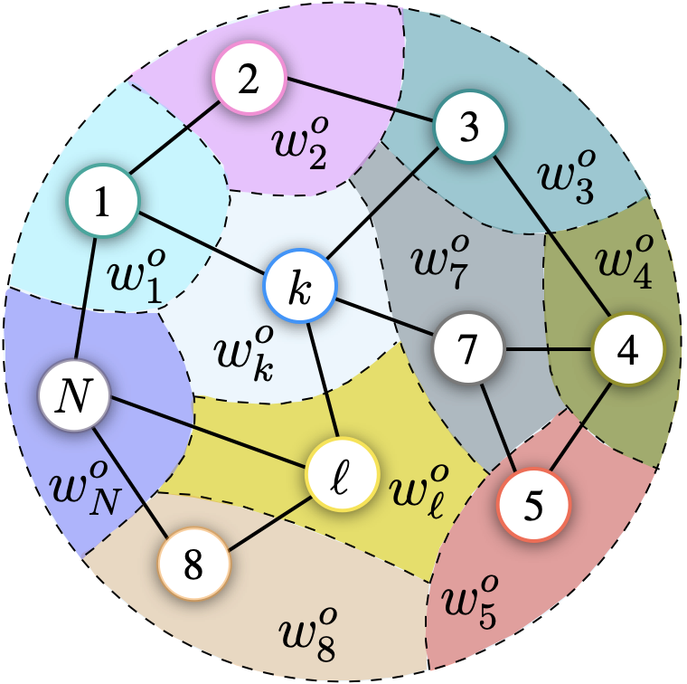
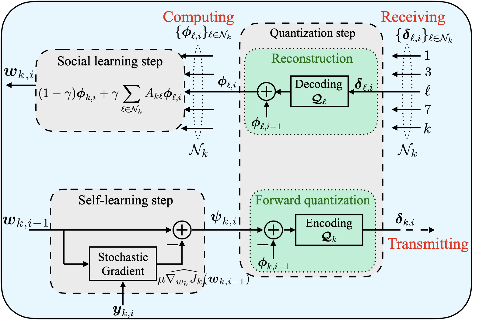
Figure 3: (Left) An illustration of a multitask network [11]. The objective at agent $k$ is to estimate $w^{o}_{k}$ (of dimension $M_{k}\times 1$), the $k$-th subvector of ${\scriptstyle\mathcal{W}}^{o}$ in (3). In this example, the neighborhood set of agent $k$ is given by $\mathcal{N}_{k}=\{1,k,3,\ell,7\}$. (Right) The implementation of the quantized multitask approach (28) at agent $k$. The quantization step consists of (i) the forward step where agent $k$ encodes the difference $\boldsymbol{\psi}_{k,i}-\boldsymbol{\phi}_{k,i-1}$ and sends the resulting vector $\boldsymbol{\delta}_{k,i}$ (sequence of symbols or bits) to its neighbors, and (ii) the reconstruction step where agent $k$ receives the encoded vectors $\{\boldsymbol{\delta}_{\ell,i}\}_{\ell\in\mathcal{N}_{k}}$ from its neighbors and decodes them according to (29) to obtain $\{\boldsymbol{\phi}_{\ell,i}\}_{\ell\in\mathcal{N}_{k}}$. The resulting vectors are then used in the social learning step (28c).

Motivated by the approaches proposed in [12, 32, 33, 34, 31, 38, 39, 37, 35, 36], we equip (1) with a quantization mechanism by proposing the following decentralized multitask learning approach–see Fig. 3:

$$\boldsymbol{\psi}_{k,i} =\boldsymbol{w}_{k,i-1}-\mu\widehat{\nabla_{w_{k}}J_{k}}(\boldsymbol{w}_{k,i-1})$$ (28a)

$$\boldsymbol{\phi}_{k,i} =\boldsymbol{\phi}_{k,i-1}+\boldsymbol{\cal{Q}}_{k}(\boldsymbol{\psi}_{k,i}-\boldsymbol{\phi}_{k,i-1})$$ (28b)

$$\boldsymbol{w}_{k,i} =(1-\gamma)\boldsymbol{\phi}_{k,i}+\gamma\sum_{\ell\in\mathcal{N}_{k}}A_{k\ell}\boldsymbol{\phi}_{\ell,i}$$ (28c)

where $\gamma\in(0,1]$ is a mixing parameter that tunes the degree of cooperation between agents, and $\boldsymbol{\cal{Q}}_{k}(\cdot)$ is a randomized quantizer satisfying Property 1. Note that, since the quantizer characteristics can vary with $k$, the randomized quantizer becomes $\boldsymbol{\cal{Q}}_{k}(\cdot)$ instead of $\boldsymbol{\cal{Q}}(\cdot)$ with a subscript $k$ added to $\boldsymbol{\cal{Q}}$. Observe that differential quantization is used in (28b) to leverage possible correlation between subsequent iterates [33]. In this case, instead of communicating compressed versions of the estimates $\boldsymbol{\psi}_{k,i}$, the prediction error $\boldsymbol{\psi}_{k,i}-\boldsymbol{\phi}_{k,i-1}$ is quantized at agent $k$ and then transmitted [12, 33, 32, 31, 38, 34, 39, 35, 36, 37]. At each iteration $i$, agent $k$ performs the forward quantization (see Fig. 3) by mapping the real-valued vector $\boldsymbol{\psi}_{k,i}-\boldsymbol{\phi}_{k,i-1}$ into a quantized vector $\boldsymbol{\delta}_{k,i}$, sends $\boldsymbol{\delta}_{k,i}$ to its neighbors through ideal communication links (i.e., it is assumed that node $k$ can transmit perfectly and reliably $\boldsymbol{\delta}_{k,i}$ to its neighbors), receives $\{\boldsymbol{\delta}_{\ell,i}\}$ from its neighbors $\ell\in\mathcal{N}_{k}$, and performs the reconstruction (see Fig. 3) on each received vector $\boldsymbol{\delta}_{\ell,i}$ by first decoding it and then computing $\{\boldsymbol{\phi}_{\ell,i}\}$ according to step (28b):

$$\boldsymbol{\phi}_{\ell,i}=\boldsymbol{\phi}_{\ell,i-1}+\boldsymbol{\cal{Q}}_{\ell}(\boldsymbol{\psi}_{\ell,i}-\boldsymbol{\phi}_{\ell,i-1}),\qquad\ell\in\mathcal{N}_{k}.$$ (29)

Observe that implementing (29) requires storing the predictors $\{\boldsymbol{\phi}_{\ell,i-1}\}_{\ell\in\mathcal{N}_{k}}$ by agent $k$. The reconstructed vectors $\{\boldsymbol{\phi}_{\ell,i}\}$ are then combined according to (28c) to produce the estimate $\boldsymbol{w}_{k,i}$. As we will see in Secs. IV and V, in the presence of relative quantization noise (i.e., when $\beta^{2}_{q}\neq 0$), the mixing parameter $\gamma$ in (28c) will be used to control the network stability. However, in the absence of relative noise (i.e., when $\beta^{2}_{q}=0$), the quantization does not affect the network stability, and the parameter $\gamma$ can be set to one.

Remark 1 (Quantized diffusion-type approach): Most prior literature on decentralized quantized learning focuses primarily on single-task consensus optimization where the objective at each agent is to estimate the same $L$-th dimensional vector $w^{o}$ given by:

$$w^{o}=\arg\min_{w}\sum_{k=1}^{N}J_{k}(w).$$ (30)

For this reason, and in order to make the paper self-contained for readers interested in problem (30), we explain in this remark how to choose the blocks $\{A_{k\ell}\}$ in (28) in order to solve problem (30) as well. In fact, by setting in (3) $P=L$ and $\mathcal{U}=\frac{1}{\sqrt{N}}(\mathds{1}_{N}\otimes I_{L})$ where $\mathds{1}_{N}$ is the $N\times 1$ vector of all ones, then solving problem (3) will be equivalent to solving the well-studied consensus problem (30). Different algorithms for solving (30) over strongly-connected networks have been proposed [8, 9, 10, 14, 13, 15]. By choosing an $N\times N$ doubly-stochastic matrix $A=[a_{k\ell}]$ satisfying:

$$a_{k\ell}\geq 0,\quad A\mathds{1}_{N}=\mathds{1}_{N},\quad\mathds{1}_{N}^{\top}A=\mathds{1}_{N}^{\top},\quad a_{k\ell}=0\text{ if }\ell\notin\mathcal{N}_{k},$$ (31)

the diffusion strategy for instance would take the form [8, 9, 10]:

$$\boldsymbol{\psi}_{k,i} =\boldsymbol{w}_{k,i-1}-\mu\widehat{\nabla_{w_{k}}J_{k}}(\boldsymbol{w}_{k,i-1})$$ (32a)

$$\boldsymbol{w}_{k,i} =\sum_{\ell\in\mathcal{N}_{k}}a_{k\ell}\boldsymbol{\psi}_{\ell,i}$$ (32b)

This strategy can be written in the form of (1) with $A_{k\ell}=a_{k\ell}I_{L}$ and $\mathcal{A}=A\otimes I_{L}$. It can be verified that, when $A$ satisfies (31) over a strongly connected network, the matrix $\mathcal{A}$ will satisfy (2). Consequently, by setting $A_{k\ell}=a_{k\ell}I_{L}$ in (28c) with a set of combination coefficients $\{a_{k\ell}\}$ satisfying (31), we obtain a new quantized diffusion-type approach for solving the consensus optimization problem (30). ∎

III-B Related work

Table I provides a list of typical compression schemes with the corresponding quantization noise parameters $\beta^{2}_{q}$ and $\sigma^{2}_{q}$. By comparing the reported schemes, we first observe that the “rand-c”, “randomized gossip”, and “gradient sparsifier” do not really quantize their input. These methods basically map a full vector into a sparse version thereof. In other words, these methods assume that the non-zero vector components are represented with very high (e.g., machine) precision, and that the overall compression gain lies in representing few entries of the input vector. For instance, under the “rand-c” scheme, $c$ randomly selected components of the input vector are encoded with very high precision ($32$ or $64$ bit are typical values for encoding a scalar), and then the resulting bits are communicated over the links in addition to the bits encoding the locations of the selected components. Such schemes should be more properly referred to as compression operators, rather than quantizers [34, 31, 12]. The idea behind sparsification operators is that, when the number of vector components is large, the gain resulting from encoding a few randomly selected components compensates for the high precision required to represent them. The QSGD scheme in Table I uses a different approximation rule. It assumes that the norm of the input vector is represented with high precision. In addition to encoding the norm, this rule requires $L$-bits to encode the signs of the vector components and $L\lceil\log_{2}(s)\rceil$ to encode the levels. It tends to be well-suited for high-dimensional settings where the number of components is large. As it can be observed from Table I, the sparsity-based schemes and the QSGD scheme have an absolute noise term $\sigma^{2}_{q}=0$. As explained in [31], neglecting the effect of $\sigma^{2}_{q}$ requires that some quantities (e.g., the norm of the input vector in QSGD) are represented with no quantization error. In comparison, the probabilistic uniform and ANQ schemes do not make any assumptions on the high-precision quantization of specific variables and have a non-zero absolute noise term $\sigma^{2}_{q}$.

A detailed analysis of the decentralized strategy (28) in the presence of both the relative (captured through $\beta^{2}_{q}$) and the absolute (captured through $\sigma^{2}_{q}$) quantization noise terms will be conducted in Sec. IV. Consequently, our results apply to a general class of quantizers satisfying Property 1, including all those listed in Table I. Compared to prior works, we provide the following advances. First, the analysis results are novel compared to the works [12, 32, 33, 5, 34, 35, 36] since we do not make any assumptions about the high-precision quantization of specific variables. Although no such assumptions are made in the work [37], the analysis there is performed in the absence of the relative quantization and gradient noise terms. Our results are also novel in comparison to [31] since we consider: i) learning under subspace constraints; ii) a stochastic optimization setting with non-diminishing step-size; iii) combination policies that can lead to non-symmetric combination matrices; and iv) a network global, as opposed to local, strong convexity condition on the individual costs – see condition (35) further ahead. Moreover, the work [31] considers only deterministic optimization and does not deal with gradient approximation or mean-square error stability. In addition, it must be noted that even the works [12, 32, 33, 5, 34, 35, 36, 37] do not consider our more general setting that simultaneously addresses i), ii), iii), and iv).

As the derivations in the next section will reveal, characterizing the behavior of the decentralized learning system under the aforementioned conditions is challenging due to at least two factors. First, the quantization noise that interferes with the operation of the algorithm. It is therefore important to assess its impact on the algorithm’s performance and stability by extending the mean-square analyses of the works [8, 9, 21, 24], which consider decentralized learning in the absence of quantization. Second, as we will see later, when we remove the common assumption about the high precision quantization of specific variables (in which case we use variable-rate quantization as suggested in Sec. II-A2), then the quantizer resolution is required to increase as $\mu\rightarrow 0$ to guarantee small mean-square errors. It therefore becomes important to establish the bit rate stability of the network, namely, to show that the average bit rate remains finite as $\mu\rightarrow 0$. To the best of our knowledge, this analysis has not been carried out before. Existing works investigate either fixed-rate quantizers [33, 32, 12, 34] or variable-rate quantizers without streaming data [31].

In summary, we provide the following main contributions.

• We propose a decentralized strategy for learning and adaptation over networks under subspace constraints. This strategy is able to operate under finite communication rate by employing differential randomized quantization.

• We provide a detailed characterization of the proposed approach for a general class of quantizers and compression operators satisfying Property 1, both in terms of mean-square stability and communication resources.

• The analysis reveals the following useful conclusions. First, the quantization error does not impair the network mean-square stability. Second, in the absence of the absolute quantization noise term, and at the expense of communicating some quantities with high precision, the iterates generated by the quantized approach (28) lead to small estimation errors on the order of $\mu$, as it happens in the unquantized case (1). In the presence of the absolute noise term, the situation becomes more challenging. The analysis reveals that, to guarantee the $O(\mu)$ mean-square-error behavior, the absolute noise term must converge to zero as $\mu\rightarrow 0$. We prove that this result can be achieved with a bit rate that remains bounded as $\mu\rightarrow 0$, despite the fact that we are requiring an increasing precision as the step-size decreases. In particular, we illustrate one useful strategy (the variable-rate quantization scheme described in Sec. II-A) that achieves the aforementioned goals.

IV Mean-square and bit rate stability analysis

IV-A Modeling assumptions

In this section, we analyze strategy (28) with a matrix $\mathcal{A}$ satisfying (2) by examining the average squared distance between $\boldsymbol{w}_{k,i}$ and $w^{o}_{k}$, namely, $\mathbb{E}\|w^{o}_{k}-\boldsymbol{w}_{k,i}\|^{2}$, under the following assumptions on the risks $\{J_{k}(\cdot)\}$, the gradient noise processes $\{\boldsymbol{s}_{k,i}(\cdot)\}$ defined by [8]:

$$\boldsymbol{s}_{k,i}(w_{k})\triangleq\nabla_{w_{k}}J_{k}(w_{k})-\widehat{\nabla_{w_{k}}J_{k}}(w_{k}),$$ (33)

and the randomized quantizers $\{\boldsymbol{\cal{Q}}_{k}(\cdot)\}$.

Assumption 1.

(Conditions on individual and aggregate costs). The individual costs $J_{k}(w_{k})$ are assumed to be twice differentiable and convex such that:

$$\lambda_{k,\min}I_{M_{k}}\leq\nabla^{2}_{w_{k}}J_{k}(w_{k})\leq\lambda_{k,\max}I_{M_{k}},$$ (34)

where $\lambda_{k,\min}\geq 0$ for $k=1,\ldots,N$. It is further assumed that, for any $\{w_{k}\in\mathbb{R}^{M_{k}}\}$, the individual costs satisfy:

$$0<\lambda_{\min}I_{P}\leq\mathcal{U}^{\top}\emph{\text{diag}}\left\{\nabla^{2}_{w_{k}}J_{k}(w_{k})\right\}_{k=1}^{N}\mathcal{U}\leq\lambda_{\max}I_{P},$$ (35)

for some positive parameters $\lambda_{\min}\leq\lambda_{\max}$. ∎

As explained in [24], condition (35) ensures that problem (3) has a unique minimizer ${\scriptstyle\mathcal{W}}^{o}$.

Assumption 2.

(Conditions on gradient noise). The gradient noise process defined in (33) satisfies for $k=1,\ldots,N$:

$$\mathbb{E}[\boldsymbol{s}_{k,i}(\boldsymbol{w}_{k,i-1})|\{{\boldsymbol{\phi}_{\ell,i-1}}\}_{\ell=1}^{N}] =0,$$ (36)

$$\mathbb{E}[\|\boldsymbol{s}_{k,i}(\boldsymbol{w}_{k,i-1})\|^{2}|\{{\boldsymbol{\phi}_{\ell,i-1}}\}_{\ell=1}^{N}] \leq\beta^{2}_{s,k}\|\widetilde{\boldsymbol{w}}_{k,i-1}\|^{2}+\sigma^{2}_{s,k},$$ (37)

for some $\beta^{2}_{s,k}\geq 0$ and $\sigma^{2}_{s,k}\geq 0$. ∎

As explained in [8, 9, 10], these conditions are satisfied by many cost functions of interest in learning and adaptation such as quadratic and regularized logistic risks. Condition (36) states that the gradient approximation should be unbiased conditioned on the predictors $\{\boldsymbol{\phi}_{\ell,i-1}\}_{\ell=1}^{N}$. Condition (37) states that the second-order moment of the gradient noise should get smaller for better estimates, since it is bounded by the squared norm of the iterate.

Assumption 3.

(Conditions on quantizers). In step (28b) of the learning approach, each agent $k$ at time $i$ applies to the difference $\boldsymbol{\chi}_{k,i}=\boldsymbol{\psi}_{k,i}-\boldsymbol{\phi}_{k,i-1}$ a randomized quantizer $\boldsymbol{\cal{Q}}_{k}(\cdot)$ satisfying Property 1 with quantization noise parameters $\beta^{2}_{q,k}$ and $\sigma^{2}_{q,k}$. It is assumed that given the past history, the randomized quantization mechanism depends only on the quantizer input $\boldsymbol{\chi}_{k,i}$. Consequently, from (6) and (7), we get:

$$\mathbb{E}[\boldsymbol{\chi}_{k,i}-\boldsymbol{\cal{Q}}_{k}(\boldsymbol{\chi}_{k,i})|\boldsymbol{h}_{i}] =\mathbb{E}[\boldsymbol{\chi}_{k,i}-\boldsymbol{\cal{Q}}_{k}(\boldsymbol{\chi}_{k,i})|\boldsymbol{\chi}_{k,i}]=0,$$ (38)

$$\mathbb{E}\left[\|\boldsymbol{\chi}_{k,i}-\boldsymbol{\cal{Q}}_{k}(\boldsymbol{\chi}_{k,i})\|^{2}|\boldsymbol{h}_{i}\right] =\mathbb{E}\left[\|\boldsymbol{\chi}_{k,i}-\boldsymbol{\cal{Q}}_{k}(\boldsymbol{\chi}_{k,i})\|^{2}|\boldsymbol{\chi}_{k,i}\right]$$

$$\leq\beta^{2}_{q,k}\|\boldsymbol{\chi}_{k,i}\|^{2}+\sigma^{2}_{q,k},$$ (39)

where $\boldsymbol{h}_{i}$ is the vector collecting all iterates generated by (28) before the quantizer is applied to $\boldsymbol{\chi}_{k,i}$, namely, $\Big{\{}\{\boldsymbol{\phi}_{\ell,j}\}_{j=0}^{i-1},\{\boldsymbol{\psi}_{\ell,j}\}_{j=1}^{i}\Big{\}}_{\ell=1}^{N}$ . ∎

Assumption 3 formalizes the quantization mechanism (which is in fact a standard mechanism in decentralized learning with randomized quantization) and highlights two fundamental relations (38) and (39) that will be useful in the technical derivations.

IV-B Network error vector recursion

In order to examine the evolution of the iterates $\boldsymbol{w}_{k,i}$ generated by algorithm (28) with respect to the minimizer ${\scriptstyle\mathcal{W}}^{o}=\text{col}\{w^{o}_{k}\}_{k=1}^{N}$ defined in (3), we start by deriving the network error vector recusion. Let $\widetilde{\boldsymbol{w}}_{k,i}=w^{o}_{k}-\boldsymbol{w}_{k,i}$, $\widetilde{\boldsymbol{\psi}}_{k,i}=w^{o}_{k}-\boldsymbol{\psi}_{k,i}$, and $\widetilde{\boldsymbol{\phi}}_{k,i}=w^{o}_{k}-\boldsymbol{\phi}_{k,i}$. Using (33) and the mean-value theorem [44, pp. 24], [8, Appendix D], we can express the stochastic gradient vector appearing in (28a) as follows:

$$\widehat{\nabla_{w_{k}}J_{k}}(\boldsymbol{w}_{k,i-1})=-\boldsymbol{H}_{k,i-1}\widetilde{\boldsymbol{w}}_{k,i-1}+b_{k}-\boldsymbol{s}_{k,i}(\boldsymbol{w}_{k,i-1})$$ (40)

where $\boldsymbol{H}_{k,i-1}\triangleq\int_{0}^{1}\nabla^{2}_{w_{k}}J_{k}(w^{o}_{k}-t\widetilde{\boldsymbol{w}}_{k,i-1})dt$ and $b_{k}\triangleq\nabla_{w_{k}}J_{k}(w^{o}_{k})$. By subtracting $w^{o}_{k}$ from both sides of (28a) and by introducing the following network quantities:

$$b \triangleq\text{col}\left\{b_{1},\ldots,b_{N}\right\},$$ (41)

$$\boldsymbol{s}_{i} \triangleq\text{col}\left\{\boldsymbol{s}_{1,i}(\boldsymbol{w}_{1,i-1}),\ldots,\boldsymbol{s}_{N,i}(\boldsymbol{w}_{N,i-1})\right\},$$ (42)

$$\boldsymbol{\cal{H}}_{i-1} \triangleq\text{diag}\left\{\boldsymbol{H}_{1,i-1},\ldots,\boldsymbol{H}_{N,i-1}\right\},$$ (43)

$$\widetilde{\boldsymbol{{\scriptstyle\mathcal{W}}}}_{i-1} \triangleq\text{col}\{\widetilde{\boldsymbol{w}}_{1,i-1},\ldots,\widetilde{\boldsymbol{w}}_{N,i-1}\},$$ (44)

we can show that the network error vector $\widetilde{\boldsymbol{\psi}}_{i}=\text{col}\{\widetilde{\boldsymbol{\psi}}_{k,i}\}_{k=1}^{N}$ evolves according to:

$$\widetilde{\boldsymbol{\psi}}_{i}=\left(I_{M}-\mu\boldsymbol{\cal{H}}_{i-1}\right)\widetilde{\boldsymbol{{\scriptstyle\mathcal{W}}}}_{i-1}-\mu\boldsymbol{s}_{i}+\mu b.$$ (45)

By subtracting $w^{o}_{k}$ from both sides of (28c), by replacing $w^{o}_{k}$ by $(1-\gamma)w^{o}_{k}+\gamma w^{o}_{k}$, and by using $w^{o}_{k}=\sum_{\ell\in\mathcal{N}_{k}}A_{k\ell}w^{o}_{\ell}$ [24, Sec. III-B], we obtain:

$$\begin{split}\widetilde{\boldsymbol{w}}_{k,i}&=(1-\gamma)\widetilde{\boldsymbol{\phi}}_{k,i}+\gamma\sum_{\ell\in\mathcal{N}_{k}}A_{k\ell}\widetilde{\boldsymbol{\phi}}_{\ell,i}.\end{split}$$ (46)

From (46), we can show that the network error vector $\widetilde{\boldsymbol{{\scriptstyle\mathcal{W}}}}_{i-1}$ in (44) evolves according to:

$$\widetilde{\boldsymbol{{\scriptstyle\mathcal{W}}}}_{i-1}=(1-\gamma)\widetilde{\boldsymbol{\phi}}_{i-1}+\gamma\mathcal{A}\widetilde{\boldsymbol{\phi}}_{i-1}=\mathcal{A}^{\prime}\widetilde{\boldsymbol{\phi}}_{i-1},$$ (47)

where

$$\widetilde{\boldsymbol{\phi}}_{i} \triangleq\text{col}\{\widetilde{\boldsymbol{\phi}}_{1,i},\ldots,\widetilde{\boldsymbol{\phi}}_{N,i}\}.$$ (48)

$$\mathcal{A}^{\prime} \triangleq(1-\gamma)I_{M}+\gamma\mathcal{A},$$ (49)

By subtracting $w^{o}_{k}$ from both sides of (28b) and by adding and subtracting $w^{o}_{k}$ to the difference $\boldsymbol{\psi}_{k,i}-\boldsymbol{\phi}_{k,i-1}$, we can write:

$$\widetilde{\boldsymbol{\phi}}_{k,i}=\widetilde{\boldsymbol{\phi}}_{k,i-1}-\boldsymbol{\cal{Q}}_{k}(\widetilde{\boldsymbol{\phi}}_{k,i-1}-\widetilde{\boldsymbol{\psi}}_{k,i}).$$ (50)

Let

$$\boldsymbol{\chi}_{k,i}=\widetilde{\boldsymbol{\phi}}_{k,i-1}-\widetilde{\boldsymbol{\psi}}_{k,i}.$$ (51)

By introducing the quantization error vector:

$$\boldsymbol{z}_{k,i}\triangleq\boldsymbol{\chi}_{k,i}-\boldsymbol{\cal{Q}}_{k}(\boldsymbol{\chi}_{k,i}),$$ (52)

we can write:

$$\widetilde{\boldsymbol{\phi}}_{k,i}=\widetilde{\boldsymbol{\psi}}_{k,i}+\boldsymbol{z}_{k,i}.$$ (53)

By combining (45), (47), and (53), we conclude that the network error vector $\widetilde{\boldsymbol{\phi}}_{i}$ in (48) evolves according to the following dynamics:

$$\boxed{\widetilde{\boldsymbol{\phi}}_{i}=\boldsymbol{\cal{B}}_{i-1}\widetilde{\boldsymbol{\phi}}_{i-1}-\mu\boldsymbol{s}_{i}+\mu b+\boldsymbol{z}_{i}}$$ (54)

where

$$\boldsymbol{\cal{B}}_{i-1} \triangleq\left(I_{M}-\mu\boldsymbol{\cal{H}}_{i-1}\right)\mathcal{A}^{\prime},$$ (55)

$$\boldsymbol{z}_{i} \triangleq\text{col}\left\{\boldsymbol{z}_{k,i}\right\}_{k=1}^{N}.$$ (56)

In Sec. IV-C, we will first establish the boundedness of $\limsup_{i\rightarrow\infty}\mathbb{E}\|\widetilde{\boldsymbol{\phi}}_{i}\|^{2}$ and then we will use relation (47) to deduce boundedness of $\limsup_{i\rightarrow\infty}\mathbb{E}\|\widetilde{\boldsymbol{{\scriptstyle\mathcal{W}}}}_{i}\|^{2}$. The analysis of recursion (54) is facilitated by transforming it to a convenient basis using the Jordan canonical decomposition of the matrix $\mathcal{A}^{\prime}$ defined in (49). Now, to exploit the eigen-structure of $\mathcal{A}^{\prime}$, we first recall that a matrix $\mathcal{A}$ satisfying the conditions in (2) (for a full-column rank semi-unitary matrix $\mathcal{U}$) has a Jordan decomposition of the form $\mathcal{A}=\mathcal{V}_{\epsilon}\Lambda_{\epsilon}\mathcal{V}_{\epsilon}^{-1}$ with [24, Lemma 2]:

$$\mathcal{V}_{\epsilon}=\left[\begin{array}[]{c|c}\mathcal{U}&\mathcal{V}_{R,\epsilon}\end{array}\right],~{}\Lambda_{\epsilon}=\left[\begin{array}[]{c|c}I_{P}&0\\ \hline\cr 0&\mathcal{J}_{\epsilon}\end{array}\right],~{}\mathcal{V}_{\epsilon}^{-1}=\left[\begin{array}[]{c}\mathcal{U}^{\top}\\ \hline\cr\mathcal{V}_{L,\epsilon}^{\top}\end{array}\right],$$ (57)

where $\mathcal{J}_{\epsilon}$ is a Jordan matrix with eigenvalues (which may be complex but have magnitude less than one) on the diagonal and $\epsilon>0$ on the super-diagonal [24, Lemma 2],[8, pp. 510]. The parameter $\epsilon$ is chosen small enough to ensure $\rho(\mathcal{J}_{\epsilon})+\epsilon\in(0,1)$ [24]. Consequently, the matrix $\mathcal{A}^{\prime}$ in (49) has a Jordan decomposition of the form $\mathcal{A}^{\prime}=\mathcal{V}_{\epsilon}\Lambda^{\prime}_{\epsilon}\mathcal{V}_{\epsilon}^{-1}$ where:

$$\Lambda^{\prime}_{\epsilon}=\left[\begin{array}[]{c|c}I_{P}&0\\ \hline\cr 0&\mathcal{J}^{\prime}_{\epsilon}\end{array}\right],\quad{\text{with }}\mathcal{J}^{\prime}_{\epsilon}\triangleq(1-\gamma)I_{M-P}+\gamma\mathcal{J}_{\epsilon}.$$ (58)

By multiplying both sides of (54) from the left by $\mathcal{V}_{\epsilon}^{-1}$ in (57), we obtain the transformed iterates and variables:

$$\mathcal{V}_{\epsilon}^{-1}\widetilde{\boldsymbol{\phi}}_{i} =\left[\begin{array}[]{c}\mathcal{U}^{\top}\widetilde{\boldsymbol{\phi}}_{i}\\ \mathcal{V}_{L,\epsilon}^{\top}\widetilde{\boldsymbol{\phi}}_{i}\end{array}\right]\triangleq\left[\begin{array}[]{c}\overline{\boldsymbol{\phi}}_{i}\\ \widecheck{\boldsymbol{\phi}}_{i}\end{array}\right],$$ (63)

$$\mathcal{V}_{\epsilon}^{-1}\boldsymbol{s}_{i} =\left[\begin{array}[]{c}\mathcal{U}^{\top}\boldsymbol{s}_{i}\\ \mathcal{V}_{L,\epsilon}^{\top}\boldsymbol{s}_{i}\end{array}\right]\triangleq\left[\begin{array}[]{c}\overline{\boldsymbol{s}}_{i}\\ \widecheck{\boldsymbol{s}}_{i}\end{array}\right],$$ (68)

$$\mathcal{V}_{\epsilon}^{-1}b =\left[\begin{array}[]{c}\mathcal{U}^{\top}b\\ \mathcal{V}_{L,\epsilon}^{\top}b\end{array}\right]\triangleq\left[\begin{array}[]{c}0\\ \widecheck{b}\end{array}\right],$$ (73)

$$\mathcal{V}_{\epsilon}^{-1}\boldsymbol{z}_{i} =\left[\begin{array}[]{c}\mathcal{U}^{\top}\boldsymbol{z}_{i}\\ \mathcal{V}_{L,\epsilon}^{\top}\boldsymbol{z}_{i}\end{array}\right]\triangleq\left[\begin{array}[]{c}\overline{\boldsymbol{z}}_{i}\\ \widecheck{\boldsymbol{z}}_{i}\end{array}\right],$$ (78)

where in (73) we used the fact that $\mathcal{U}^{\top}b=0$ as shown in [24, Sec. III-B]. In particular, the transformed components $\overline{\boldsymbol{\phi}}_{i}$ and ${\widecheck{\boldsymbol{\phi}}}_{i}$ evolve according to the recursions:

$$\overline{\boldsymbol{\phi}}_{i} =(I_{P}-\mu\boldsymbol{\cal{D}}_{11,i-1})\overline{\boldsymbol{\phi}}_{i-1}-\mu\boldsymbol{\cal{D}}_{12,i-1}\widecheck{\boldsymbol{\phi}}_{i-1}+\overline{\boldsymbol{z}}_{i}-\mu\overline{\boldsymbol{s}}_{i}$$ (79)

$${\widecheck{\boldsymbol{\phi}}}_{i} =(\mathcal{J}^{\prime}_{\epsilon}-\mu\boldsymbol{\cal{D}}_{22,i-1})\widecheck{\boldsymbol{\phi}}_{i-1}-\mu\boldsymbol{\cal{D}}_{21,i-1}\overline{\boldsymbol{\phi}}_{i-1}+\widecheck{\boldsymbol{z}}_{i}+\mu\widecheck{b}-\mu\widecheck{\boldsymbol{s}}_{i}$$ (80)

where

$$\boldsymbol{\cal{D}}_{11,i-1} \triangleq\mathcal{U}^{\top}\boldsymbol{\cal{H}}_{i-1}\mathcal{U},$$ (81)

$$\boldsymbol{\cal{D}}_{12,i-1} \triangleq\mathcal{U}^{\top}\boldsymbol{\cal{H}}_{i-1}\mathcal{V}_{R,\epsilon}\mathcal{J}_{\epsilon}^{\prime},$$ (82)

$$\boldsymbol{\cal{D}}_{21,i-1} \triangleq\mathcal{V}_{L,\epsilon}^{\top}\boldsymbol{\cal{H}}_{i-1}\mathcal{U},$$ (83)

$$\boldsymbol{\cal{D}}_{22,i-1} \triangleq\mathcal{V}_{L,\epsilon}^{\top}\boldsymbol{\cal{H}}_{i-1}\mathcal{V}_{R,\epsilon}\mathcal{J}_{\epsilon}^{\prime}.$$ (84)

In the following, we shall establish the mean-square-error stability of algorithm (28). The analysis will reveal the influence of the step-size $\mu$, the mixing parameter $\gamma$, and the quantization noise (through $\{\beta^{2}_{q,k},\sigma^{2}_{q,k}\}$) on the network mean-square-error stability and performance, and will provide insights into the design of effective quantizers for decentralized learning under subspace constraints.

IV-C Mean-square-error stability

Theorem 1.

(Mean-square-error stability). Consider a network of $N$ agents running the quantized decentralized strategy (28) under Assumptions 1, 2, and 3, with a matrix $\mathcal{A}$ satisfying (2) for an $M\times P$ (with $P\ll M$) full-column rank semi-unitary matrix $\mathcal{U}$. Let $\gamma\in(0,1]$ be such that:

$$0<\gamma<\min\left\{1,\frac{1-(\rho(\mathcal{J}_{\epsilon})+\epsilon)}{4v_{1}^{2}v_{2}^{2}\beta^{2}_{q,\max}(\rho(I-\mathcal{J}_{\epsilon})+\epsilon)^{2}}\right\}.$$ (85)

where $v_{1}=\|\mathcal{V}_{\epsilon}^{-1}\|$, $v_{2}=\|\mathcal{V}_{\epsilon}\|$, and ${\beta}_{q,\max}^{2}\triangleq\max_{1\leq k\leq N}\{{\beta}^{2}_{q,k}\}$. Then, the network is mean-square-error stable for sufficiently small step-size $\mu$, namely, it holds that:

$$\limsup_{i\rightarrow\infty}\mathbb{E}\|w^{o}_{k}-\boldsymbol{w}_{k,i}\|^{2}=\delta O(\mu)+\overline{\sigma}^{2}_{q}O(\mu^{-1}),$$ (86)

for $k=1,\ldots,N$ and where $\delta$ is a constant given by:

$$\delta\triangleq 2v_{1}^{2}\overline{\sigma}^{2}_{s}+\frac{3\|\widecheck{b}\|^{2}}{1-\|\mathcal{J}^{\prime}_{\epsilon}\|}+\beta^{2}_{q,\max}v_{1}^{2}v_{2}^{2}(2v_{1}^{2}\overline{\sigma}^{2}_{s}+12\|\widecheck{b}\|^{2}),$$ (87)

$\overline{\sigma}^{2}_{s}=\sum_{k=1}^{N}\sigma_{s,k}^{2}$, $\widecheck{b}=O(1)$ is given by (73), and $\overline{\sigma}^{2}_{q}=\sum_{k=1}^{N}{\sigma}^{2}_{q,k}$. Convergence to the steady-state value (86) is linear at a rate given by:

$$\begin{split}\rho\left(\Gamma\right)\leq\max\Big{\{}&1-\mu\sigma_{11}+O(\mu^{2}),\\ &\|\mathcal{J}_{\epsilon}^{\prime}\|+\kappa\|I-\mathcal{J}_{\epsilon}^{\prime}\|^{2}+O(\mu)\Big{\}}<1,\end{split}$$ (88)

for some positive constants $\sigma_{11}$ and $\kappa$.

Proof.

See Appendix A. ∎

While expression (86) in Theorem 1 reveals the influence of the step-size $\mu$, the quantization noise (captured by $\{\overline{\sigma}^{2}_{q},\beta^{2}_{q,\max}\}$), and the gradient noise (captured by $\overline{\sigma}^{2}_{s}$) on the steady-state mean-square error, expression (85) reveals the influence of the relative quantization noise term (captured by $\beta^{2}_{q,\max}$) on the network stability. One main conclusion stemming from expression (86) in Theorem 1 is that the mean-square-error contains an $O(\mu)$ term, which is classically encountered in the unquantized case, plus an $O(\mu^{-1})$ term, which can be problematic in the small step-size regime (if the quantity $\overline{\sigma}^{2}_{q}=\sum_{k=1}^{N}{\sigma}^{2}_{q,k}$ is not coupled with $\mu$). Since $\overline{\sigma}^{2}_{q}$ depends on the quantizers’ absolute noise components $\{\sigma^{2}_{q,k}\}$, this issue can be addressed by ensuring that $\sigma^{2}_{q,k}\propto\mu^{2}$. In this way, we would recover the small estimation error result $\limsup_{i\rightarrow\infty}\mathbb{E}\|w^{o}_{k}-\boldsymbol{w}_{k,i}\|^{2}=O(\mu)$ observed in the unquantized case.

However, this setup requires a careful inspection since small values of $\sigma^{2}_{q,k}$ imply small quantization errors, which might in principle require large bit rates. Consequently, in the small step-size regime ($\mu\rightarrow 0$), the bit rate might increase without bound when $\sigma^{2}_{q,k}\propto\mu^{2}$. Our goal then becomes to find a quantization scheme that achieves the classical small estimation error result $\limsup_{i\rightarrow\infty}\mathbb{E}\|w^{o}_{k}-\boldsymbol{w}_{k,i}\|^{2}=O(\mu)$ while guaranteeing that the bit rate stays bounded as $\mu\rightarrow 0$. In the next theorem, we will be able to show that the variable-rate scheme illustrated in Sec. II-A achieves both objectives. This theoretical finding will be further illustrated in the simulation section VI-A.

IV-D Bit rate stability

Before establishing the bit rate stability, we recall that, at each iteration $i$ and agent $k$, the quantizer input is given by $\boldsymbol{\psi}_{k,i}-\boldsymbol{\phi}_{k,i-1}$, which is equal to the vector $\boldsymbol{\chi}_{k,i}$ in (51). Consequently, from (27), the bit rate at agent $k$ and iteration $i$ is given by:

$${{r}_{k,i}}=\log_{2}(3)\sum_{j=1}^{M_{k}}\left(1+\mathbb{E}\left[\left\lceil\log_{2}(|\boldsymbol{n}([\boldsymbol{\chi}_{k,i}]_{j})|+1)\right\rceil\right]\right),$$ (89)

where $[\boldsymbol{\chi}_{k,i}]_{j}$ denotes the $j$-th entry of the vector $\boldsymbol{\chi}_{k,i}$.

Theorem 2.

(Bit rate stability). Assume that each agent $k$ employs the randomized quantizer with the non-linearities given by (18), and with the parameters $\omega_{k}$ and $\eta_{k}$ scaling according to:

$$\omega_{k}=c,\qquad\eta_{k}\propto\mu,$$ (90)

where $c$ is a constant independent of $\mu$, and where the symbol $\propto$ hides a proportionality constant independent of $\mu$. First, under conditions (90), we have:

$$\sigma^{2}_{q,k}\propto\mu^{2}.$$ (91)

Second, in steady-state, the average number of bits at agent $k$ stays bounded as $\mu\rightarrow 0$, namely,

$$\limsup_{i\rightarrow\infty}\,{r}_{k,i}=O(1).$$ (92)

Proof.

See Appendix B. ∎

To be concrete, we deemed it useful to focus in Theorem 2 on the logarithmic companding rule (18). However, it should be noted that the proof in Appendix B can be extended to handle more general non-linear functions.

V Theorems 1 and 2: insights and observations

The fundamental conclusion emerging from Theorems 1 and 2 is that, when compared with (1), and when the quantizers are properly designed, the quantized approach (28) can guarantee a finite average bit rate whilst still ensuring small estimation errors on the order of $\mu$. As detailed in the following, there are further insights that can be gained from the theorems.

First, note that in the absence of quantization, the analysis allows us to recover the mean-square-error stability result established in [24, Theorem 1] where it was shown that $\limsup_{i\rightarrow\infty}\mathbb{E}\|w^{o}_{k}-\boldsymbol{w}_{k,i}\|^{2}=O(\mu)$ for all $k$ and for $\gamma=1$. To see this, we just set to $0$ the quantization noise parameters $\{\beta_{q,\max}^{2},\overline{\sigma}^{2}_{q}\}$ in Theorem 1.

Second, from our analysis, it is possible to explain the bit rate stability result. Consider, for simplicity, the dithered uniform quantizer from Table I. Then, setting $\sigma^{2}_{q,k}\propto\mu^{2}$ is equivalent to requiring that the quantization step-size $\Delta$ is proportional to $\mu$. Our analysis reveals that, when $\Delta\propto\mu$, the differential input $\boldsymbol{\chi}_{k,i}=\boldsymbol{\psi}_{k,i}-\boldsymbol{\phi}_{k,i-1}$ in (28b) is on the order of $\mu$ at the steady-state. In this setting, i) the effective range of the inputs used in the differential quantizer scheme vanishes as $O(\mu)$ when $\mu\rightarrow 0$, and ii) the quantizer resolution $\Delta\propto\mu$ scales proportionally to the effective range of the quantizer input. Notably, Theorem 2 reveals that the variable-rate scheme is able to adapt the number of bits to this effective range, in such a way that the expected bit rate stays bounded as $\mu\rightarrow 0$.

Third, we conclude from Theorem 1 that, while a value $\gamma=1$ could lead to network instability when $\beta^{2}_{q,\max}\neq 0$, this conclusion does not hold when $\beta^{2}_{q,\max}=0$. In other words, the absolute quantization noise component does not affect the network stability, and the network remains stable for sufficiently small step-size $\mu$ when $\gamma=1$.

Fourth, by noting that step (28b) can be written alternatively as:

$$\boldsymbol{\phi}_{k,i}=\boldsymbol{\psi}_{k,i}-\boldsymbol{z}_{k,i},$$ (93)

with $\boldsymbol{z}_{k,i}$ given by (52), it can be observed that the impact of quantization in (28c) is similar to the impact of exchanging information over the communication links in the presence of additive noise processes since step (28c) can be written alternatively as (for $\gamma=1$):

$$\boldsymbol{w}_{k,i}=\sum_{\ell\in\mathcal{N}_{k}}A_{k\ell}(\boldsymbol{\psi}_{\ell,i}-\boldsymbol{z}_{\ell,i}).$$ (94)

Therefore, in the absence of the relative quantization noise term (i.e., when $\beta^{2}_{q,\max}=0$), we obtain a setting similar to the one previously considered in the context of single-task [28] and multititask [29] estimation over mean-square-error networks in the presence of noisy links. However, notice that the analysis in [28] and [29] is limited to LMS diffusion algorithms, does not exploit the randomized quantizers design, and does not investigate the average bit rate stability.

Fifth, observe that in the absence of absolute quantization noise term, i.e., when $\overline{\sigma}^{2}_{q}=0$, we obtain:

$$\limsup_{i\rightarrow\infty}\mathbb{E}\|w^{o}_{k}-\boldsymbol{w}_{k,i}\|^{2}=O(\mu).$$ (95)

Thus, the relative quantization noise component does not affect the $O(\mu)$ small estimation error result, but affects the network stability through condition (85). Regarding the bit rate, as it can be observed from Table I (column 5, rows 4–7), the reported quantization schemes are characterized by a fixed bit-budget that is independent of the quantizer input, but depends on the high-precision quantization parameter $B_{\text{HP}}$. The theoretical result (95) will be illustrated in Sec. VI-A by considering the QSGD quantizer of Table I (row 7).

Finally, and before discussing the stability condition (85), we note that the parameter $\gamma$ allows to control $\rho(\mathcal{A}^{\prime}-\mathcal{P}_{{\scriptscriptstyle\mathcal{U}}})$ (i.e., the spectral radius of the matrix $\mathcal{A}^{\prime}-\mathcal{P}_{{\scriptscriptstyle\mathcal{U}}}$), and consequently, the speed of convergence of $(\mathcal{A}^{\prime})^{i}$ to $\mathcal{P}_{{\scriptscriptstyle\mathcal{U}}}$ [24, Lemma 2]. To see this, note that (by using the Jordan decomposition of the matrix $\mathcal{A}^{\prime}$):

$$\mathcal{A}^{\prime}-\mathcal{P}_{{\scriptscriptstyle\mathcal{U}}}=\mathcal{V}_{\epsilon}\left[\begin{array}[]{c|c}0&0\\ \hline\cr 0&\mathcal{J}^{\prime}_{\epsilon}\end{array}\right]\mathcal{V}_{\epsilon}^{-1},$$ (96)

from which we obtain $\rho(\mathcal{A}^{\prime}-\mathcal{P}_{{\scriptscriptstyle\mathcal{U}}})=\rho(\mathcal{J}^{\prime}_{\epsilon})\overset{\eqref{eq: equation to bound rho J prime}}{\leq}(1-\gamma)+\gamma\rho(\mathcal{J}_{\epsilon})$ where $\rho(\mathcal{J}_{\epsilon})\in(0,1)$ and $\gamma\in(0,1]$. Thus, the larger the mixing parameter $\gamma$ is, the smaller $\rho(\mathcal{A}^{\prime}-\mathcal{P}_{{\scriptscriptstyle\mathcal{U}}})$ tends to be, and consequently, the faster the convergence of $(\mathcal{A}^{\prime})^{i}$ to $\mathcal{P}_{{\scriptscriptstyle\mathcal{U}}}$ will be. Now, returning to the stability condition (85), besides requiring $\gamma\in(0,1]$, the mixing parameter $\gamma$ must be chosen smaller than a value that is inversely proportional to $\beta^{2}_{q,\max}$. Thus, the larger $\beta^{2}_{q,\max}$ is, the tighter the upper bound in (85) is, and the smaller $\gamma$ should be. If we consider for instance the QSGD quantizer from Table I, it can be observed that the smaller the number of levels $s$ is, i.e., the smaller the number of used bits is, the larger $\beta^{2}_{q,k}$ is. Consequently, the larger $\beta^{2}_{q,k}$ is, the farther the agents (seeking to converge to $\text{Range}(\mathcal{U})$) can get from the subspace due to the quantization noise, and thus, the mixing parameter $\gamma$ must be chosen small enough to ensure that the quantization noise perturbations will not affect the network stability.

VI Simulation results

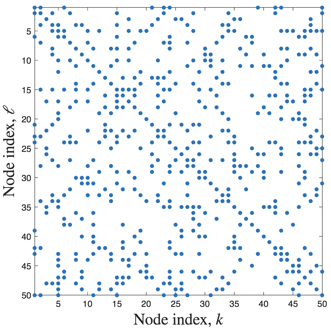
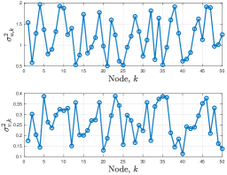
Figure 4: Experimental setup. (Left) Link matrix ($N=50$ nodes). (Right) Regressor and noise variances.

We apply strategy (28) to a network of $N=50$ nodes with the link matrix shown in Fig. 4 (left). Each agent is subjected to streaming data $\{\boldsymbol{d}_{k}(i),\boldsymbol{u}_{k,i}\}$ assumed to satisfy a linear regression model of the form [8]:

$$\boldsymbol{d}_{k}(i)=\boldsymbol{u}_{k,i}^{\top}w^{\star}_{k}+\boldsymbol{v}_{k}(i),$$ (97)

for some unknown $L\times 1$ vector $w^{\star}_{k}$ with $\boldsymbol{v}_{k}(i)$ denoting a zero-mean measurement noise and $L=5$. A mean-square-error cost of the form $J_{k}(w_{k})=\frac{1}{2}\mathbb{E}|\boldsymbol{d}_{k}(i)-\boldsymbol{u}_{k,i}^{\top}w_{k}|^{2}$ is associated with each agent $k$. The regressor and noise processes $\{\boldsymbol{u}_{k,i},\boldsymbol{v}_{k}(i)\}$ are assumed to be zero-mean Gaussian with: i) $\mathbb{E}\boldsymbol{u}_{k,i}\boldsymbol{u}_{\ell,i}^{\top}=R_{u,k}=\sigma^{2}_{u,k}I_{L}$ if $k=\ell$ and zero otherwise; ii) $\mathbb{E}\boldsymbol{v}_{k}(i)\boldsymbol{v}_{\ell}(i)=\sigma^{2}_{v,k}$ if $k=\ell$ and zero otherwise; and iii) $\boldsymbol{u}_{k,i}$ and $\boldsymbol{v}_{k}(i)$ are independent of each other. The variances $\sigma^{2}_{u,k}$ and $\sigma^{2}_{v,k}$ are illustrated in Fig. 4 (right). The signal ${\scriptstyle\mathcal{W}}^{\star}=\text{col}\{w^{\star}_{1},\ldots,w^{\star}_{N}\}$ is generated by smoothing a signal ${\scriptstyle\mathcal{W}}_{o}$, which is randomly generated from the Gaussian distribution $\mathcal{N}(0.4\times\mathds{1}_{NL},I_{NL})$, by a graph diffusion kernel with $\tau=3$ – see [25, Sec. IV] for more details on the smoothing process. The matrix $\mathcal{U}$ is generated according to $\mathcal{U}=U\otimes I_{L}$ where $U=[u_{1}~{}u_{2}]$, and $u_{1}$ and $u_{2}$ are the first two eigenvectors of the graph Laplacian $\mathscr{L}$. The Laplacian matrix is generated according to $\mathscr{L}=\text{diag}\{C\mathds{1}_{N}\}-C$ where $C$ is the $N\times N$ weighted adjacency matrix chosen such that the $(k,\ell)-$th entry $[C]_{k\ell}=0.1$ if $\ell\in\mathcal{N}_{k}$ and $0$ otherwise. The combination matrix $\mathcal{A}$ satisfying the conditions in (2) and having the same structure as the graph is found by following the same approach as in [45].

VI-A Effect of the small step-size parameter

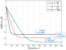
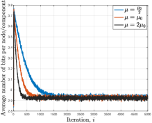
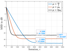
Figure 5: Network performance w.r.t. ${\scriptstyle\mathcal{W}}^{o}$ in (3) for three different values of the step-size ($\mu_{0}=0.003$). In the left and middle plots, the probabilistic ANQ quantizer of Example 2 is employed. (Left) Evolution of the MSD learning curves. (Middle) Evolution of the average number of bits per node, per component, when the variable-rate scheme described in Sec. II-A is used to encode the difference $\boldsymbol{\chi}_{k,i}=\boldsymbol{\psi}_{k,i}-\boldsymbol{\phi}_{k,i-1}$ in (28b). (Right) Evolution of the MSD learning curves when the QSGD quantizer (with $s=2$) of Table I is used.

In Fig. 5 (left), we report the network mean-square-deviation (MSD) learning curves:

$$\text{MSD}(i)=\frac{1}{N}\sum_{k=1}^{N}\mathbb{E}\|w^{o}_{k}-\boldsymbol{w}_{k,i}\|^{2}$$ (98)

for 3 different values of the step-size $\mu$. The results were averaged over 100 Monte-Carlo runs. We used the probabilistic ANQ quantizer of Example 2 with $\omega_{k}=0.25$ and $\eta_{k}=\frac{\mu}{\sqrt{2L}}$. This choice ensures that the quantizer settings of Theorem 2 are satisfied. We set $\gamma=0.88$. We observe that, in steady-state, the network MSD increases by approximately $3$dB when $\mu$ goes from $\mu_{0}$ to $2\mu_{0}$. This means that the performance is on the order of $\mu$, as expected from the discussion in Sec. V since in the simulations the absolute noise component is such that $\sigma^{2}_{q,k}=\mu^{2}$. In Fig. 5 (middle), we report the average number of bits per node, per component, computed according to:

$$R(i)=\frac{1}{N}\sum_{k=1}^{N}\frac{1}{L}r_{k,i},$$ (99)

where $r_{k,i}$ is the bit rate given by (89), which is associated with the encoding of the difference vector $\boldsymbol{\chi}_{k,i}=\boldsymbol{\psi}_{k,i}-\boldsymbol{\phi}_{k,i-1}$ transmitted by agent $k$ at iteration $i$ according to (28b). As it can be observed, and thanks to the variable-rate quantization, a finite average number of bits is guaranteed (approximately 2.9 bits/component/iteration are required on average in steady-state). Moreover, it can be observed that the average number of bits scales coherently with the distortion scaling law induced by $\mu$. That is, a smaller MSD in steady-state would require using a larger number of bits, and vice versa.

For comparison purposes, we report in Fig. 5 (right) the MSD learning curves when the QSGD quantizer of Table I (row 7) is employed instead of the probabilistic ANQ. Apart from the quantizer scheme, the same settings as above were assumed. For the QSGD scheme, we set the number of quantization levels $s$ to $2$. As it can be observed, this choice allows us to compare the average number of bits for the ANQ and QSGD quantizers for similar values of steady-state MSD. From Table I (row 7, column 5), the bit-budget required to encode a $5\times 1$ vector using the QSGD scheme ($s=2$) is given by $B_{\text{HP}}+10$. Now, by replacing $B_{\text{HP}}$ by 32 (since we are performing the experiments on MATLAB 2022a which uses 32 bits to represent a floating number in single-precision), we find that the QSGD quantizer requires, at each iteration $i$, an average number of bits per node, per component, equal to $\frac{42}{5}=8.4$, which is almost three times higher than the one obtained in steady-state when the probabilistic ANQ is used. This is expected since the QSGD scheme requires encoding the norm of the input vector with very high precision.

Note that, since the results of Theorems 1 and 2 hold for any $M\times P$ full-column rank semi-unitary matrix $\mathcal{U}$, similar observations will hold true when applying the quantized approach (28) to solve general constrained optimization problems of the form (3). In the supplementary material, we illustrate this fact by considering a simulation similar to the one considered in the current section VI-A, but instead we consider solving consensus optimization (30) by choosing $\mathcal{U}=\frac{1}{\sqrt{N}}(\mathds{1}_{N}\otimes I_{L})$.

VI-B Rate-distortion curves

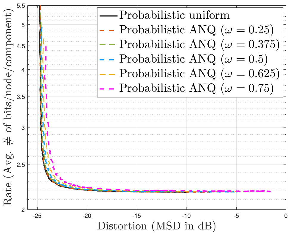
Figure 6: (Left) Rate-distortion curves for the probabilistic uniform and ANQ.

In order to examine the performance of the proposed learning strategy, it is necessary to consider both the attained learning error (MSD) and the associated bit expense. This gives rise to a rate-distortion curve, where the rate quantifies the bit budget and the MSD quantifies the distortion. In Fig. 6, we illustrate the rate-distortion curves for probabilistic uniform and ANQ (for different values of the parameter $\omega$). We set $\mu=0.003$ and $\gamma=0.88$. For the probabilistic uniform quantizer, each point of the rate/distortion curve corresponds to one value of the quantization step $\Delta$. In the example, we selected $200$ values of $\Delta$, uniformly sampled in the interval $[0,0.1]$. For each value of $\Delta$ (i.e., each point of the curve), the resulting MSD (distortion) and average number of bits/node/component (rate) were obtained by averaging the instantaneous mean-square-deviation MSD$(i)$ in (98) and averaging the number of bits $R(i)$ in (99) over 500 samples after convergence of the algorithm (the expectations in (98) and (89) are estimated empirically over $50$ Monte Carlo runs). For the probabilistic ANQ scheme, we draw three curves corresponding to different values of the parameter $\omega$. For each curve, the different rate/distortion pairs correspond to $200$ values of the parameter $\eta$, uniformly sampled in the interval $[0,0.5]$. The trade-off between rate and distortion can be observed from Fig. 6, namely, as the rate decreases, the distortion increases, and vice versa. For the ANQ, we further observe that the curves move away from the uniform case as $\omega$ increases, indicating a superior performance of the uniform probabilistic quantizer. In other words, the simulations show that in the considered example no advantage is obtained by employing non-uniform quantization. One useful interpretation for this behavior is as follows. In the theory of quantization, non-uniform quantizers are typically employed in a fixed-rate context, where the number of bits is determined in advance and does not depend on the input value. Under this setting, allocating high-resolution quantization intervals where the random variable is more likely to be observed provides some advantage in terms of distortion, given the available fixed rate. However, in our case, we are considering a variable-rate quantizer that changes the number of bits depending on the input value. For example, when the quantizer input $x$ belongs to a narrower quantization interval (i.e., smaller distortion), the variable-rate scheme allocates a higher number of bits. This somehow nullifies the distortion gain since we are allocating more bits. Therefore, allocating non-uniform intervals and then adapting the variable rate does not seem rewarding when compared to a uniform quantizer. This bears some similarity to what happens in the theory of quantization when one employs a fixed-rate quantizer followed by an entropy encoder. In this case, the possible advantages of non-uniform quantizers are nullified by the entropy encoder, and it is well known that (in the high resolution regime) the uniform quantizer is the best choice [46].

VI-C Tracking ability

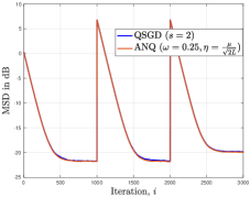
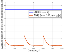
Figure 7: Network performance in non-stationary environment (i.e., the solution ${\scriptstyle\mathcal{W}}^{o}$ in (3) is changing over time due to changes in the individual costs $\{J_{k}(w_{k})\}$) when the probabilistic ANQ quantizer of Example 2 and the QSGD quantizer of Table I are used. (Left) Evolution of the MSD learning curves. (Right) Evolution of the average number of bits per node, per component. The variable-rate scheme described in Sec. II-A is used in the probabilistic ANQ case.

To illustrate the tracking ability of the quantized approach (28), we modify $w^{\star}_{k}$ in (97) at time instants $1000$ and $2000$ by modifying ${\scriptstyle\mathcal{W}}_{o}$ such that ${\scriptstyle\mathcal{W}}_{o}$ is randomly generated from $\mathcal{N}(1.4\times\mathds{1}_{NL},I_{NL})$ at $i=1000$ and from $\mathcal{N}(2.4\times\mathds{1}_{NL},I_{NL})$ at $i=2000$. Apart from varying ${\scriptstyle\mathcal{W}}_{o}$ (and, consequently, ${\scriptstyle\mathcal{W}}^{o}$ in (3)) and from fixing the step-size $\mu$ to $0.006$, the same settings as in Sec. VI-A were assumed. The resulting MSD learning curves and average number of bits/node/component curves are reported in Fig. 7 (left) and (right), respectively, for both the probabilistic ANQ and the QSGD quantizers. As it can be observed, approach (28) is able to track changes in the solution of the constrained optimization problem (3) despite quantization.

VII Conclusion

In this work, we considered inference problems over networks where agents have individual parameter vectors to estimate subject to subspace constraints that require the parameters across the network to lie in low-dimensional subspaces. The constrained subspace problem includes standard consensus optimization as a special case, and allows for more general task relatedness models such as multitask smoothness. To alleviate the communication bottleneck resulting from the exchange of the intermediate estimates among agents over many iterations, we proposed a new decentralized strategy relying on differential randomized quantizers. We studied its mean-square-error stability in the presence of both relative and absolute quantization noise terms. The analysis framework is general enough to cover many typical examples of probabilistic quantizers such as QSGD quantizer, gradient sparsifier, uniform or dithered quantizer, and non-uniform compandor. We showed that, for small step-sizes, and under some conditions on the quantizers (captured by the terms $\beta^{2}_{q,k},\sigma^{2}_{q,k}$), on the network topology (captured by the eigendecomposition of the combination matrix $\mathcal{A}$), and on the mixing parameter $\gamma$, the decentralized quantized approach is able to converge in the mean-square-error sense within $O(\mu)$ from the solution of the constrained optimization problem, despite the gradient and quantization noises.

Appendix A Mean-square-error analysis

We consider the transformed iterates $\overline{\boldsymbol{\phi}}_{i}$ and $\widecheck{\boldsymbol{\phi}}_{i}$ in (79) and (80), respectively. Computing the second-order moment of both sides of (79), we get:

$$\begin{split}\mathbb{E}\|\overline{\boldsymbol{\phi}}_{i}\|^{2}=&\mathbb{E}\|(I_{P}-\mu\boldsymbol{\cal{D}}_{11,i-1})\overline{\boldsymbol{\phi}}_{i-1}-\mu\boldsymbol{\cal{D}}_{12,i-1}\widecheck{\boldsymbol{\phi}}_{i-1}\|^{2}\\ &+\mu^{2}\mathbb{E}\|\overline{\boldsymbol{s}}_{i}\|^{2}+\mathbb{E}\|\overline{\boldsymbol{z}}_{i}\|^{2},\end{split}$$ (100)

where, from Assumptions 3 and 2 on the quantization and gradient noise processes, we used the fact that:

$$\mathbb{E}[\boldsymbol{x}_{i-1}^{\top}\overline{\boldsymbol{z}}_{i}] =\mathbb{E}\left[\mathbb{E}[\boldsymbol{x}_{i-1}^{\top}\overline{\boldsymbol{z}}_{i}|\boldsymbol{h}_{i}]\right]=\mathbb{E}\left[\boldsymbol{x}_{i-1}^{\top}\mathbb{E}[\overline{\boldsymbol{z}}_{i}|\boldsymbol{h}_{i}]\right]=0$$ (101)

$$\mathbb{E}[\boldsymbol{x}_{i-1}^{\top}\overline{\boldsymbol{s}}_{i}] =\mathbb{E}\left[\mathbb{E}\left[\boldsymbol{x}_{i-1}^{\top}\overline{\boldsymbol{s}}_{i}\Big{|}\{{\boldsymbol{\phi}_{\ell,i-1}}\}_{\ell=1}^{N}\right]\right]$$

$$=\mathbb{E}\left[\boldsymbol{x}_{i-1}^{\top}\mathbb{E}\left[\overline{\boldsymbol{s}}_{i}\Big{|}\{{\boldsymbol{\phi}_{\ell,i-1}}\}_{\ell=1}^{N}\right]\right]=0$$ (102)

$$\mathbb{E}[\overline{\boldsymbol{s}}_{i}^{\top}\overline{\boldsymbol{z}}_{i}] =\mathbb{E}\left[\mathbb{E}[\overline{\boldsymbol{s}}_{i}^{\top}\overline{\boldsymbol{z}}_{i}|\boldsymbol{h}_{i}]\right]=\mathbb{E}\left[\overline{\boldsymbol{s}}_{i}^{\top}\mathbb{E}[\overline{\boldsymbol{z}}_{i}|\boldsymbol{h}_{i}]\right]=0$$ (103)

with $\boldsymbol{x}_{i-1}=(I_{P}-\mu\boldsymbol{\cal{D}}_{11,i-1})\overline{\boldsymbol{\phi}}_{i-1}-\mu\boldsymbol{\cal{D}}_{12,i-1}\widecheck{\boldsymbol{\phi}}_{i-1}$. Using similar arguments, we can also show that:

$$\begin{split}\mathbb{E}\|\widecheck{\boldsymbol{\phi}}_{i}\|^{2}=&\mathbb{E}\|(\mathcal{J}^{\prime}_{\epsilon}-\mu\boldsymbol{\cal{D}}_{22,i-1})\widecheck{\boldsymbol{\phi}}_{i-1}-\mu\boldsymbol{\cal{D}}_{21,i-1}\overline{\boldsymbol{\phi}}_{i-1}+\mu\widecheck{b}\|^{2}\\ &+\mu^{2}\mathbb{E}\|\widecheck{\boldsymbol{s}}_{i}\|^{2}+\mathbb{E}\|\widecheck{\boldsymbol{z}}_{i}\|^{2}.\end{split}$$ (104)

Before proceeding, we show that, for small enough $\epsilon$, the $2-$induced matrix norm of $\mathcal{J}^{\prime}_{\epsilon}$ in (58) satisfies $\|\mathcal{J}^{\prime}_{\epsilon}\|\in(0,1)$. This property will be used in the subsequent analysis. To establish the property, and by following similar arguments as in [8, pp. 516–517], we can first show that the block diagonal matrix $\mathcal{J}^{\prime}_{\epsilon}$, which is given by (58), satisfies:

$$\|\mathcal{J}_{\epsilon}^{\prime}\|^{2}\leq(\rho(\mathcal{J}^{\prime}_{\epsilon})+\gamma\epsilon)^{2}.$$ (105)

From (58), we can also show that:

$$\rho(\mathcal{J}^{\prime}_{\epsilon})\leq(1-\gamma)+\gamma\rho(\mathcal{J}_{\epsilon}).$$ (106)

Using the fact that $\rho(\mathcal{J}_{\epsilon})\in(0,1)$ from [24, Lemma 2] and the fact that $\gamma\in(0,1]$, we obtain $\rho(\mathcal{J}^{\prime}_{\epsilon})\in(0,1)$. Since $\rho(\mathcal{J}^{\prime}_{\epsilon})+\gamma\epsilon$ is non-negative, by replacing (106) into (105), we obtain:

$$\begin{split}\|\mathcal{J}_{\epsilon}^{\prime}\|&\leq(1-\gamma)+\gamma\rho(\mathcal{J}_{\epsilon})+\gamma\epsilon\\ &=1-\gamma(1-\rho(\mathcal{J}_{\epsilon})-\epsilon).\end{split}$$ (107)

This identity will also be used in the subsequent analysis. Regarding the block diagonal matrix $I-\mathcal{J}_{\epsilon}^{\prime}$, which will appear in the following analysis, we can establish (by following similar arguments as in [8, pp. 516–517]):

$$\|I-\mathcal{J}_{\epsilon}^{\prime}\|^{2}\overset{\eqref{eq: jordan decomposition of A'}}{=}\|\gamma(I-\mathcal{J}_{\epsilon})\|^{2}=\gamma^{2}\|I-\mathcal{J}_{\epsilon}\|^{2}\leq\gamma^{2}(\rho(I-\mathcal{J}_{\epsilon})+\epsilon)^{2},$$ (108)

where $\rho(I-\mathcal{J}_{\epsilon})\in(0,2)$ since $\rho(\mathcal{J}_{\epsilon})\in(0,1)$.

Now, returning to the error recursions (100) and (104), and using similar arguments as those used to establish inequalities (119) and (124) in [24, Appendix D], we can show that:

$$\begin{split}\mathbb{E}\|\overline{\boldsymbol{\phi}}_{i}\|^{2}\leq&(1-\mu\sigma_{11})\mathbb{E}\|\overline{\boldsymbol{\phi}}_{i-1}\|^{2}+\frac{\mu\sigma_{12}^{2}}{\sigma_{11}}\mathbb{E}\|\widecheck{\boldsymbol{\phi}}_{i-1}\|^{2}+\\ &\mathbb{E}\|\overline{\boldsymbol{z}}_{i}\|^{2}+\mu^{2}\mathbb{E}\|\overline{\boldsymbol{s}}_{i}\|^{2},\end{split}$$ (109)

and

$$\begin{split}&\mathbb{E}\|\widecheck{\boldsymbol{\phi}}_{i}\|^{2}\leq\left(\|\mathcal{J}^{\prime}_{\epsilon}\|+\frac{3\mu^{2}\sigma_{22}^{2}}{1-\|\mathcal{J}^{\prime}_{\epsilon}\|}\right)\mathbb{E}\|\widecheck{\boldsymbol{\phi}}_{i-1}\|^{2}+\\ &\left(\frac{3\mu^{2}\sigma_{21}^{2}}{1-\|\mathcal{J}^{\prime}_{\epsilon}\|}\right)\mathbb{E}\|\overline{\boldsymbol{\phi}}_{i-1}\|^{2}+\left(\frac{3\mu^{2}}{1-\|\mathcal{J}^{\prime}_{\epsilon}\|}\right)\|\widecheck{b}\|^{2}+\mathbb{E}\|\widecheck{\boldsymbol{z}}_{i}\|^{2}+\mu^{2}\mathbb{E}\|\widecheck{\boldsymbol{s}}_{i}\|^{2}\end{split}$$ (110)

for some positive constant $\sigma_{11}$ and non-negative constants $\sigma_{12},\sigma_{21}$, and $\sigma_{22}$ independent of $\mu$. As it can be seen from (73), $\widecheck{b}=\mathcal{V}_{L,\epsilon}^{\top}b$ depends on $b$ in (41), which is defined in terms of the gradients $\{\nabla_{w_{k}}J_{k}(w^{o}_{k})\}$. Since the costs $J_{k}(w_{k})$ are twice differentiable, then $\|b\|^{2}$ is bounded and we obtain $\|\widecheck{b}\|^{2}=O(1)$.

For the gradient noise terms, by following similar arguments as in [8, Chapter 9], [24, Appendix D] and by using Assumption 2, we can show that:

$$\mathbb{E}\|\overline{\boldsymbol{s}}_{i}\|^{2}+\mathbb{E}\|\widecheck{\boldsymbol{s}}_{i}\|^{2}=\mathbb{E}\|\mathcal{V}_{\epsilon}^{-1}\boldsymbol{s}_{i}\|^{2}\leq v_{1}^{2}\beta_{s,\max}^{2}\mathbb{E}\|\widetilde{\boldsymbol{{\scriptstyle\mathcal{W}}}}_{i-1}\|^{2}+v_{1}^{2}\overline{\sigma}^{2}_{s},$$ (111)

where $v_{1}=\|\mathcal{V}_{\epsilon}^{-1}\|$, $\beta_{s,\max}^{2}=\max_{1\leq k\leq N}\beta_{s,k}^{2}$, and $\overline{\sigma}^{2}_{s}=\sum_{k=1}^{N}\sigma^{2}_{s,k}$. Using expression (47) and the Jordan decomposition of the matrix $\mathcal{A}^{\prime}$ in (49), we obtain:

$$\begin{split}&\mathbb{E}\|\overline{\boldsymbol{s}}_{i}\|^{2}+\mathbb{E}\|\widecheck{\boldsymbol{s}}_{i}\|^{2}\\ &\leq v_{1}^{2}\beta_{s,\max}^{2}\mathbb{E}\|\mathcal{A}^{\prime}\widetilde{\boldsymbol{\phi}}_{i-1}\|^{2}+v_{1}^{2}\overline{\sigma}^{2}_{s}\\ &\leq v_{1}^{2}\beta_{s,\max}^{2}\mathbb{E}\|\mathcal{V}_{\epsilon}\Lambda^{\prime}(\mathcal{V}_{\epsilon}^{-1}\widetilde{\boldsymbol{\phi}}_{i-1})\|^{2}+v_{1}^{2}\overline{\sigma}^{2}_{s}\\ &\leq v_{1}^{2}\beta_{s,\max}^{2}v_{2}^{2}(\mathbb{E}\|\overline{\boldsymbol{\phi}}_{i-1}\|^{2}+\mathbb{E}\|\widecheck{\boldsymbol{\phi}}_{i-1}\|^{2})+v_{1}^{2}\overline{\sigma}^{2}_{s},\end{split}$$ (112)

where $v_{2}=\|\mathcal{V}_{\epsilon}\|$.

Using the bound (112) into (109) and (110), we obtain:

$$\begin{split}&\mathbb{E}\|\overline{\boldsymbol{\phi}}_{i}\|^{2}\leq(1-\mu\sigma_{11}+\mu^{2}v_{1}^{2}\beta_{s,\max}^{2}v_{2}^{2})\mathbb{E}\|\overline{\boldsymbol{\phi}}_{i-1}\|^{2}+\\ &\left(\frac{\mu\sigma_{12}^{2}}{\sigma_{11}}+\mu^{2}v_{1}^{2}\beta_{s,\max}^{2}v_{2}^{2}\right)\mathbb{E}\|\widecheck{\boldsymbol{\phi}}_{i-1}\|^{2}+\mathbb{E}\|\overline{\boldsymbol{z}}_{i}\|^{2}+\mu^{2}v_{1}^{2}\overline{\sigma}^{2}_{s},\end{split}$$ (113)

and

$$\begin{split}&\mathbb{E}\|\widecheck{\boldsymbol{\phi}}_{i}\|^{2}\leq\left(\|\mathcal{J}^{\prime}_{\epsilon}\|+\frac{3\mu^{2}\sigma_{22}^{2}}{1-\|\mathcal{J}^{\prime}_{\epsilon}\|}+\mu^{2}v_{1}^{2}\beta_{s,\max}^{2}v_{2}^{2}\right)\mathbb{E}\|\widecheck{\boldsymbol{\phi}}_{i-1}\|^{2}+\\ &\left(\frac{3\mu^{2}\sigma_{21}^{2}}{1-\|\mathcal{J}^{\prime}_{\epsilon}\|}+\mu^{2}v_{1}^{2}\beta_{s,\max}^{2}v_{2}^{2}\right)\mathbb{E}\|\overline{\boldsymbol{\phi}}_{i-1}\|^{2}+\left(\frac{3\mu^{2}}{1-\|\mathcal{J}^{\prime}_{\epsilon}\|}\right)\|\widecheck{b}\|^{2}\\ &\quad+\mathbb{E}\|\widecheck{\boldsymbol{z}}_{i}\|^{2}+\mu^{2}v_{1}^{2}\overline{\sigma}^{2}_{s}.\end{split}$$ (114)

Now, for the quantization noise, we have:

$$\begin{split}\mathbb{E}\|\overline{\boldsymbol{z}}_{i}\|^{2}+\mathbb{E}\|\widecheck{\boldsymbol{z}}_{i}\|^{2}=\mathbb{E}\|\mathcal{V}_{\epsilon}^{-1}\boldsymbol{z}_{i}\|^{2}\overset{\eqref{eq: equation for z}}{\leq}v_{1}^{2}\left(\sum_{k=1}^{N}\mathbb{E}\|\boldsymbol{z}_{k,i}\|^{2}\right).\end{split}$$ (115)

From (52) and Assumption 3, and since $\boldsymbol{\chi}_{k,i}=\widetilde{\boldsymbol{\phi}}_{k,i-1}-\widetilde{\boldsymbol{\psi}}_{k,i}$, we can write:

$$\begin{split}\mathbb{E}\|\boldsymbol{z}_{k,i}\|^{2}\leq{\beta}^{2}_{q,k}\mathbb{E}\|\widetilde{\boldsymbol{\phi}}_{k,i-1}-\widetilde{\boldsymbol{\psi}}_{k,i}\|^{2}+{\sigma}^{2}_{q,k},\end{split}$$ (116)

and, therefore,

$$\begin{split}\mathbb{E}\|\boldsymbol{z}_{i}\|^{2}\leq{\beta}_{q,\max}^{2}\mathbb{E}\|\widetilde{\boldsymbol{\phi}}_{i-1}-\widetilde{\boldsymbol{\psi}}_{i}\|^{2}+\overline{\sigma}^{2}_{q},\end{split}$$ (117)

where ${\beta}_{q,\max}^{2}=\max_{1\leq k\leq N}\{{\beta}^{2}_{q,k}\}$ and $\overline{\sigma}^{2}_{q}=\sum_{k=1}^{N}{\sigma}^{2}_{q,k}$. Since the analysis is facilitated by transforming the network vectors into the Jordan decomposition basis of the matrix $\mathcal{A}^{\prime}$, we proceed by noting that the term $\mathbb{E}\|\boldsymbol{z}_{i}\|^{2}$ can be bounded as follows:

$$\begin{split}\mathbb{E}\|\boldsymbol{z}_{i}\|^{2}&\overset{\eqref{eq: expression 4}}{\leq}{\beta}_{q,\max}^{2}\mathbb{E}\|\mathcal{V}_{\epsilon}\mathcal{V}_{\epsilon}^{-1}(\widetilde{\boldsymbol{\phi}}_{i-1}-\widetilde{\boldsymbol{\psi}}_{i})\|^{2}+\overline{\sigma}^{2}_{q}\\ &~{}\leq{\beta}_{q,\max}^{2}\|\mathcal{V}_{\epsilon}\|^{2}\mathbb{E}\|\mathcal{V}_{\epsilon}^{-1}(\widetilde{\boldsymbol{\phi}}_{i-1}-\widetilde{\boldsymbol{\psi}}_{i})\|^{2}+\overline{\sigma}^{2}_{q}\\ &~{}\leq v_{2}^{2}{\beta}_{q,\max}^{2}[\mathbb{E}\|\overline{\boldsymbol{\chi}}_{i}\|^{2}+\mathbb{E}\|\widecheck{\boldsymbol{\chi}}_{i}\|^{2}]+\overline{\sigma}^{2}_{q},\end{split}$$ (118)

where

$$\overline{\boldsymbol{\chi}}_{i} \triangleq\mathcal{U}^{\top}(\widetilde{\boldsymbol{\phi}}_{i-1}-\widetilde{\boldsymbol{\psi}}_{i}),$$ (119)

$$\widecheck{\boldsymbol{\chi}}_{i} \triangleq\mathcal{V}_{L,\epsilon}^{\top}(\widetilde{\boldsymbol{\phi}}_{i-1}-\widetilde{\boldsymbol{\psi}}_{i}).$$ (120)

Therefore, by combining (115) and (118), we obtain:

$$\begin{split}\mathbb{E}\|\overline{\boldsymbol{z}}_{i}\|^{2}+\mathbb{E}\|\widecheck{\boldsymbol{z}}_{i}\|^{2}\leq v_{1}^{2}v_{2}^{2}{\beta}_{q,\max}^{2}[\mathbb{E}\|\overline{\boldsymbol{\chi}}_{i}\|^{2}+\mathbb{E}\|\widecheck{\boldsymbol{\chi}}_{i}\|^{2}]+v_{1}^{2}\overline{\sigma}^{2}_{q}.\end{split}$$ (121)

We focus now on deriving the network vector transformed recursions $\overline{\boldsymbol{\chi}}_{i}$ and $\widecheck{\boldsymbol{\chi}}_{i}$. Subtracting $\widetilde{\boldsymbol{\phi}}_{i-1}$ from both sides of (45) and using (47), we obtain:

$$\begin{split}\widetilde{\boldsymbol{\phi}}_{i-1}-\widetilde{\boldsymbol{\psi}}_{i}=(I_{M}-\mathcal{A}^{\prime}+\mu\boldsymbol{\cal{H}}_{i-1}\mathcal{A}^{\prime})\widetilde{\boldsymbol{\phi}}_{i-1}+\mu\boldsymbol{s}_{i}-\mu b.\end{split}$$ (122)

By multiplying both sides of (122) by $\mathcal{V}_{\epsilon}^{-1}$ and by using (63)–(73), (81)–(84), and the Jordan decomposition of the matrix $\mathcal{A}^{\prime}$, we obtain:

$$\begin{split}\left[\begin{array}[]{c}\overline{\boldsymbol{\chi}}_{i}\\ \widecheck{\boldsymbol{\chi}}_{i}\end{array}\right]=&\left[\begin{array}[]{cc}\mu\boldsymbol{\cal{D}}_{11,i-1}&\mu\boldsymbol{\cal{D}}_{12,i-1}\\ \mu\boldsymbol{\cal{D}}_{21,i-1}&I_{M-P}-\mathcal{J}^{\prime}_{\epsilon}+\mu\boldsymbol{\cal{D}}_{22,i-1}\end{array}\right]\left[\begin{array}[]{c}\overline{\boldsymbol{\phi}}_{i-1}\\ \widecheck{\boldsymbol{\phi}}_{i-1}\end{array}\right]\\ &+\mu\left[\begin{array}[]{c}\overline{\boldsymbol{s}}_{i}\\ \widecheck{\boldsymbol{s}}_{i}\end{array}\right]-\mu\left[\begin{array}[]{c}0\\ \widecheck{b}\end{array}\right].\end{split}$$ (123)

Again, by using similar arguments as those used to establish inequalities (119) and (124) in [24, Appendix D] and by using Jensen’s inequalities $\|x+y\|^{2}\leq 2\|x\|^{2}+2\|y\|^{2}$ and $\|x+y+z\|^{2}\leq 3\|x\|^{2}+3\|y\|^{2}+3\|z\|^{2}$, we can verify that:

$$\begin{split}\mathbb{E}\|\overline{\boldsymbol{\chi}}_{i}\|^{2}\leq&2\mu^{2}\sigma^{2}_{11}\mathbb{E}\|\overline{\boldsymbol{\phi}}_{i-1}\|^{2}+2\mu^{2}\sigma_{12}^{2}\mathbb{E}\|\widecheck{\boldsymbol{\phi}}_{i-1}\|^{2}+\mu^{2}\mathbb{E}\|\overline{\boldsymbol{s}}_{i}\|^{2},\end{split}$$ (124)

and

$$\begin{split}&\mathbb{E}\|\widecheck{\boldsymbol{\chi}}_{i}\|^{2}\leq 6\mu^{2}\sigma^{2}_{21}\mathbb{E}\|\overline{\boldsymbol{\phi}}_{i-1}\|^{2}+\\ &2\left(\|I-\mathcal{J}_{\epsilon}^{\prime}\|^{2}+3\mu^{2}\sigma^{2}_{22}\right)\mathbb{E}\|\widecheck{\boldsymbol{\phi}}_{i-1}\|^{2}+6\mu^{2}\|\widecheck{b}\|^{2}+\mu^{2}\mathbb{E}\|\widecheck{\boldsymbol{s}}_{i}\|^{2}.\end{split}$$ (125)

By combining expressions (124) and (125), we obtain:

$$\begin{split}\mathbb{E}\|\overline{\boldsymbol{\chi}}_{i}\|^{2}&+\mathbb{E}\|\widecheck{\boldsymbol{\chi}}_{i}\|^{2}\leq\left(2\mu^{2}\sigma^{2}_{11}+6\mu^{2}\sigma^{2}_{21}\right)\mathbb{E}\|\overline{\boldsymbol{\phi}}_{i-1}\|^{2}+\\ &\left(2\mu^{2}\sigma_{12}^{2}+2\|I-\mathcal{J}_{\epsilon}^{\prime}\|^{2}+6\mu^{2}\sigma^{2}_{22}\right)\mathbb{E}\|\widecheck{\boldsymbol{\phi}}_{i-1}\|^{2}+\\ &~{}6\mu^{2}\|\widecheck{b}\|^{2}+\mu^{2}\left(\mathbb{E}\|\overline{\boldsymbol{s}}_{i}\|^{2}+\mathbb{E}\|\widecheck{\boldsymbol{s}}_{i}\|^{2}\right).\end{split}$$ (126)

Now, by using the bound (112) in (126), we obtain:

$$\begin{split}&\mathbb{E}\|\overline{\boldsymbol{\chi}}_{i}\|^{2}+\mathbb{E}\|\widecheck{\boldsymbol{\chi}}_{i}\|^{2}\leq 6\mu^{2}\|\widecheck{b}\|^{2}+\mu^{2}v_{1}^{2}\overline{\sigma}^{2}_{s}+\\ &\left(2\mu^{2}\sigma^{2}_{11}+6\mu^{2}\sigma^{2}_{21}+\mu^{2}v_{1}^{2}\beta_{s,\max}^{2}v_{2}^{2}\right)\mathbb{E}\|\overline{\boldsymbol{\phi}}_{i-1}\|^{2}+\\ &\left(2\mu^{2}\sigma_{12}^{2}+2\|I-\mathcal{J}_{\epsilon}^{\prime}\|^{2}+6\mu^{2}\sigma^{2}_{22}+\mu^{2}v_{1}^{2}\beta_{s,\max}^{2}v_{2}^{2}\right)\mathbb{E}\|\widecheck{\boldsymbol{\phi}}_{i-1}\|^{2}.\end{split}$$ (127)

Using (127) and (121) in (113) and (114), we finally find that the variances of $\overline{\boldsymbol{\phi}}_{i}$ and $\widecheck{\boldsymbol{\phi}}_{i}$ are coupled and recursively bounded as:

$$\left[\begin{array}[]{c}\mathbb{E}\|\overline{\boldsymbol{\phi}}_{i}\|^{2}\\ \mathbb{E}\|\widecheck{\boldsymbol{\phi}}_{i}\|^{2}\end{array}\right]\preceq\Gamma\left[\begin{array}[]{c}\mathbb{E}\|\overline{\boldsymbol{\phi}}_{i-1}\|^{2}\\ \mathbb{E}\|\widecheck{\boldsymbol{\phi}}_{i-1}\|^{2}\end{array}\right]+\left[\begin{array}[]{c}e+v_{1}^{2}\overline{\sigma}^{2}_{q}\\ f+v_{1}^{2}\overline{\sigma}^{2}_{q}\end{array}\right],$$ (128)

where $\Gamma$ is the $2\times 2$ matrix given by:

$$\Gamma=\left[\begin{array}[]{cc}a&b\\ c&d\end{array}\right],$$ (129)

with

$$a =1-\mu\sigma_{11}+O(\mu^{2})={\color[rgb]{0,0,0}1-\Theta(\mu)},$$ (130)

$$b =2v_{1}^{2}v_{2}^{2}{\beta}_{q,\max}^{2}\|I-\mathcal{J}_{\epsilon}^{\prime}\|^{2}+O(\mu),$$ (131)

$$c =O(\mu^{2}),$$ (132)

$$d =\|\mathcal{J}^{\prime}_{\epsilon}\|+2v_{1}^{2}v_{2}^{2}{\beta}_{q,\max}^{2}\|I-\mathcal{J}_{\epsilon}^{\prime}\|^{2}+O(\mu^{2}),$$ (133)

$$e \triangleq\mu^{2}\left(6\|\widecheck{b}\|^{2}v_{1}^{2}v_{2}^{2}{\beta}_{q,\max}^{2}+v_{1}^{2}\overline{\sigma}^{2}_{s}v_{1}^{2}v_{2}^{2}{\beta}_{q,\max}^{2}+v_{1}^{2}\overline{\sigma}^{2}_{s}\right),$$ (134)

$$f \triangleq\mu^{2}\left(\frac{3\|\widecheck{b}\|^{2}}{1-\|\mathcal{J}^{\prime}_{\epsilon}\|}+6v_{1}^{2}v_{2}^{2}{\beta}_{q,\max}^{2}\|\widecheck{b}\|^{2}+v_{1}^{4}\overline{\sigma}^{2}_{s}v_{2}^{2}{\beta}_{q,\max}^{2}+v_{1}^{2}\overline{\sigma}^{2}_{s}\right)$$ (135)

where the notation $g(\mu)=\Theta(\mu)$ signifies that there exists a positive constant $c$ such that $\lim_{\mu\rightarrow 0}\frac{g(\mu)}{\mu}=c$.

If the matrix $\Gamma$ is stable, i.e., $\rho(\Gamma)<1$, then by iterating (128), we arrive at:

$$\limsup_{i\rightarrow\infty}\left[\begin{array}[]{c}\mathbb{E}\|\overline{\boldsymbol{\phi}}_{i}\|^{2}\\ \mathbb{E}\|\widecheck{\boldsymbol{\phi}}_{i}\|^{2}\end{array}\right]\preceq(I-\Gamma)^{-1}\left[\begin{array}[]{c}e+v_{1}^{2}\overline{\sigma}^{2}_{q}\\ f+v_{1}^{2}\overline{\sigma}^{2}_{q}\end{array}\right].$$ (140)

As we will see in the following, for some given data settings (captured by $\{\sigma_{11}^{2},\sigma_{12}^{2},\sigma_{21}^{2},\sigma_{22}^{2},\beta^{2}_{s,\max},\overline{\sigma}^{2}_{s}\}$), small step-size parameter $\mu$, network topology (captured by the matrix $\mathcal{A}$ and its eigendecomposition $\{v_{1}^{2},v_{2}^{2},\mathcal{J}_{\epsilon}\}$), and quantizer settings (captured by $\{\beta_{q,\max}^{2},\overline{\sigma}^{2}_{q}\}$), the stability of $\Gamma$ can be controlled by the mixing parameter $\gamma$ used in step (28c). As it can be observed from (58), (107), and (108), this parameter influences $\|\mathcal{J}^{\prime}_{\epsilon}\|^{2}$ and $\|I-\mathcal{J}^{\prime}_{\epsilon}\|^{2}$. Generally speaking, and since the spectral radius of a matrix is upper bounded by its $1-$norm, the matrix $\Gamma$ is stable if:

$$\rho(\Gamma)\leq\max\{|a|+|c|,|b|+|d|\}<1.$$ (141)

Since $\sigma_{11}>0$ and $\gamma\neq 0$, a sufficiently small $\mu$ can make $|a|+|c|$ strictly smaller than 1. For $|b|+|d|$, observe that if the mixing parameter $\gamma$ is chosen such that:

$$\|\mathcal{J}^{\prime}_{\epsilon}\|+4v_{1}^{2}v_{2}^{2}\beta^{2}_{q,\max}\|I-\mathcal{J}^{\prime}_{\epsilon}\|^{2}<1,$$ (142)

then $|b|+|d|$ can be made strictly smaller than one for sufficiently small $\mu$. It is therefore clear that the RHS of (141) can be made strictly smaller than one for sufficiently small $\mu$ and for a mixing parameter $\gamma\neq 0$ satisfying condition (142). Now, to derive condition (85) on the mixing parameter $\gamma$, we start by noting that the LHS of (142) can be upper bounded by:

$$\begin{split}&\|\mathcal{J}^{\prime}_{\epsilon}\|+4v_{1}^{2}v_{2}^{2}\beta^{2}_{q,\max}\|I-\mathcal{J}^{\prime}_{\epsilon}\|^{2}\\ &\overset{\eqref{eq: bound on norm of J' epsilon},\eqref{eq: bound on I-J epsilon'}}{\leq}1-\gamma(1-\rho(\mathcal{J}_{\epsilon})-\epsilon)+4v_{1}^{2}v_{2}^{2}\beta^{2}_{q,\max}\gamma^{2}(\rho(I-\mathcal{J}_{\epsilon})+\epsilon)^{2}.\end{split}$$ (143)

The upper bound in the above inequality is guaranteed to be strictly smaller than 1 if:

$$4v_{1}^{2}v_{2}^{2}\beta^{2}_{q,\max}\gamma^{2}(\rho(I-\mathcal{J}_{\epsilon})+\epsilon)^{2}-\gamma(1-\rho(\mathcal{J}_{\epsilon})-\epsilon)<0.$$ (144)

Now, by using the above condition and the fact that $\gamma$ must be in $(0,1]$, we obtain condition (85).

Under condition (85), $\rho(\Gamma)<1$, and consequently, the matrix $\Gamma$ is stable. Moreover, it holds that:

$$(I-\Gamma)=\left[\begin{array}[]{cc}{\color[rgb]{0,0,0}\Theta(\mu)}&O(1)\\ O(\mu^{2})&{\color[rgb]{0,0,0}\Theta(1)}\end{array}\right],$$ (145)

and:

$$(I-\Gamma)^{-1}=\left[\begin{array}[]{cc}{\color[rgb]{0,0,0}\Theta(\mu^{-1})}&O(\mu^{-1})\\ O(\mu)&{\color[rgb]{0,0,0}\Theta(1)}\end{array}\right].$$ (146)

Now, using (134), (135), and (146) into (140), we arrive at:

$$\limsup_{i\rightarrow\infty}\left[\begin{array}[]{c}\mathbb{E}\|\overline{\boldsymbol{\phi}}_{i}\|^{2}\\ \mathbb{E}\|\widecheck{\boldsymbol{\phi}}_{i}\|^{2}\end{array}\right]\preceq$$ (149)

$$\left[\begin{array}[]{c}\beta^{2}_{q,\max}\overline{\sigma}^{2}_{s}O(\mu)+\beta^{2}_{q,\max}\|\widecheck{b}\|^{2}O(\mu)+\overline{\sigma}^{2}_{s}O(\mu)+\|\widecheck{b}\|^{2}O(\mu)+\overline{\sigma}^{2}_{q}O(\mu^{-1})\\ O(\mu^{2})+\overline{\sigma}^{2}_{q}O(1)\end{array}\right]$$ (152)

By noting that:

$$\limsup_{i\rightarrow\infty}\mathbb{E}\|\widetilde{\boldsymbol{{\scriptstyle\mathcal{W}}}}_{i}\|^{2} \overset{\eqref{eq: wt in terms of phi}}{=}\limsup_{i\rightarrow\infty}\mathbb{E}\|\mathcal{A}^{\prime}\widetilde{\boldsymbol{\phi}}_{i}\|^{2}$$

$$=\limsup_{i\rightarrow\infty}\mathbb{E}\|\mathcal{V}_{\epsilon}\Lambda_{\epsilon}^{\prime}\mathcal{V}_{\epsilon}^{-1}\widetilde{\boldsymbol{\phi}}_{i}\|^{2}$$

$$\leq\limsup_{i\rightarrow\infty}\|\mathcal{V}_{\epsilon}\|^{2}\|\Lambda_{\epsilon}^{\prime}\|^{2}[\mathbb{E}\|\overline{\boldsymbol{\phi}}_{i}\|^{2}+\mathbb{E}\|\widecheck{\boldsymbol{\phi}}_{i}\|^{2}],$$ (153)

and by using (149), we can finally conclude (86).

Appendix B Bit Rate stability

Equation (91) follows straightforwardly from (20). Regarding (92), we first note from (18) that $g(t)\geq 0$ for non-negative arguments, and that:

$$|\boldsymbol{n}(t)|=\boldsymbol{n}(t)\leq\lfloor g(t)\rfloor+1\leq g(t)+1,\qquad\text{for }t\geq 0$$ (154)

where the first inequality follows from (9) and (10), and the fact that the random index $\boldsymbol{n}(t)$ can be either equal to $\lfloor g(t)\rfloor$ or to the integer $\lfloor g(t)+1\rfloor$. The second inequality follows from the definition of the floor operator. Likewise, for $t<0$, we obtain:

$$\boldsymbol{n}(t)\geq\lfloor g(t)\rfloor=\lfloor-g(-t)\rfloor=-\lceil g(-t)\rceil\geq-g(-t)-1.$$ (155)

Combining (154) and (155), we obtain:

$$|\boldsymbol{n}(t)|\leq g(|t|)+1,$$ (156)

and, consequently, we can write:

$$\lceil\log_{2}(|\boldsymbol{n}(t)|+1)\rceil\leq\log_{2}(|\boldsymbol{n}(t)|+1)+1\leq\log_{2}(g(|t|)+2)+1.$$ (157)

Now, from (18), we can write:

$$\log_{2}(g(|t|)+2)=\log_{2}\left(\frac{\ln\left(1+\displaystyle{\frac{\omega}{\eta}}\sqrt{t^{2}}\right)}{2\ln\left(\omega+\sqrt{1+\omega^{2}}\right)}+2\right),$$ (158)

which can be verified to be a concave function w.r.t. to the argument $t^{2}$. Therefore, if we consider a random input $\boldsymbol{t}$ in (157), take the expectation, and use Jensen’s inequality, we get:

$$\mathbb{E}\left[\lceil\log_{2}(|\boldsymbol{n}(\boldsymbol{t})|+1)\rceil\right]\leq\log_{2}\left(\frac{\ln\left(1+\displaystyle{\frac{\omega}{\eta}}\sqrt{\mathbb{E}[\boldsymbol{t}^{2}]}\right)}{2\ln\left(\omega+\sqrt{1+\omega^{2}}\right)}+2\right)+1.$$ (159)

By choosing $\boldsymbol{t}=[\boldsymbol{\chi}_{k,i}]_{j}$ in (159) and by using the fact that $([\boldsymbol{\chi}_{k,i}]_{j})^{2}\leq\|\boldsymbol{\chi}_{k,i}\|^{2}$, we can upper bound the individual summand in (89) by the quantity:

$$2+\log_{2}\left(\frac{\ln\left(1+\displaystyle{\frac{\omega}{\eta}}\sqrt{\mathbb{E}\|\boldsymbol{\chi}_{k,i}\|^{2}}\right)}{2\ln\left(\omega+\sqrt{1+\omega^{2}}\right)}+2\right).$$ (160)

By taking the limit superior of (127) as $i\rightarrow\infty$ and by using (149), we obtain $l_{k}=\limsup_{i\rightarrow\infty}\mathbb{E}\|\boldsymbol{\chi}_{k,i}\|^{2}=O(\mu^{2})$. Consequently, we find that the limit superior of (160) as $i\rightarrow\infty$ is:

$$2+\log_{2}\left(\frac{\ln\left(1+\displaystyle{\frac{\omega}{\eta}}\sqrt{l_{k}}\right)}{2\ln\left(\omega+\sqrt{1+\omega^{2}}\right)}+2\right).$$ (161)

where we have used the fact that the function in (160) is continuous and increasing in the argument $\mathbb{E}\|\boldsymbol{\chi}_{k,i}\|^{2}$ and, hence, the limit superior is preserved. Under the conditions in (90), the above quantity is $O(1)$, and consequently, the rate in (89) satisfies (92).

Supplementary material

B-A Decentralized consensus optimization

In this section, we illustrate the performance of the quantized decentralized approach (28) when applied to solve the consensus optimization problem (30). The network of $N=50$ nodes with the link matrix shown in Fig. 4 (left) is considered. Each agent is subjected to streaming data $\{\boldsymbol{d}_{k}(i),\boldsymbol{u}_{k,i}\}$ satisfying the linear regression model (97) for some unknown $L\times 1$ vector $w^{\star}_{k}$ with $\boldsymbol{v}_{k}(i)$ denoting a zero-mean measurement noise and $L=5$. A mean-square-error cost of the form $J_{k}(w_{k})=\frac{1}{2}\mathbb{E}|\boldsymbol{d}_{k}(i)-\boldsymbol{u}_{k,i}^{\top}w_{k}|^{2}$ is associated with each agent $k$. Similarly to the settings in Sec. VI, the processes $\{\boldsymbol{u}_{k,i},\boldsymbol{v}_{k}(i)\}$ are assumed to be zero-mean Gaussian with: i) $\mathbb{E}\boldsymbol{u}_{k,i}\boldsymbol{u}_{\ell,i}^{\top}=R_{u,k}=\sigma^{2}_{u,k}I_{L}$ if $k=\ell$ and zero otherwise; ii) $\mathbb{E}\boldsymbol{v}_{k}(i)\boldsymbol{v}_{\ell}(i)=\sigma^{2}_{v,k}$ if $k=\ell$ and zero otherwise; and iii) $\boldsymbol{u}_{k,i}$ and $\boldsymbol{v}_{k}(i)$ are independent of each other. The variances $\sigma^{2}_{u,k}$ and $\sigma^{2}_{v,k}$ are illustrated in Fig. 4 (right). The signal ${\scriptstyle\mathcal{W}}^{\star}=\text{col}\{w^{\star}_{1},\ldots,w^{\star}_{N}\}$ is also generated by smoothing a signal ${\scriptstyle\mathcal{W}}_{o}$, which is randomly generated from the Gaussian distribution $\mathcal{N}(0.4\times\mathds{1}_{NL},I_{NL})$, by a graph diffusion kernel with $\tau=3$. The matrix $\mathcal{U}$ is generated according to $\mathcal{U}=U\otimes I_{L}$ where $U=\frac{1}{\sqrt{N}}\mathds{1}_{N}$. The combination matrix $\mathcal{A}$ satisfying the conditions in (2) and having the same structure as the graph is found by following the same approach as in [45].

In Fig. 8 (left), we report the network mean-square-deviation (MSD) learning curves for 3 different values of the step-size $\mu$. The results were averaged over 100 Monte-Carlo runs. We used the probabilistic ANQ quantizer of Example 2 with $\omega_{k}=0.25$ and $\eta_{k}=\frac{\mu}{\sqrt{2L}}$. We set $\gamma=0.88$. We observe that, in steady-state, the network MSD increases by approximately $3$dB when $\mu$ goes from $\mu_{0}$ to $2\mu_{0}$. This means that the performance is on the order of $\mu$. In Fig. 8 (middle), we report the average number of bits per node, per component, computed according to (99). As it can be observed, and thanks to the variable-rate quantization, a finite average number of bits is guaranteed (approximately 2.8 bits/component/iteration are required on average in steady-state).

We report in Fig. 8 (right) the MSD learning curves when the QSGD quantizer of Table I (row 7) is employed instead of the probabilistic ANQ. Apart from the quantizer scheme, the same settings as above were assumed. For the QSGD scheme, we set the number of quantization levels $s$ to $2$. As it can be observed, this choice allows us to compare the average number of bits for the ANQ and QSGD quantizers for similar values of steady-state MSD. From Table I (row 7, column 5), the bit-budget required to encode a $5\times 1$ vector using the QSGD scheme ($s=2$) is given by $B_{\text{HP}}+10$. Now, by replacing $B_{\text{HP}}$ by 32 (since we are performing the experiments on MATLAB 2022a which uses 32 bits to represent a floating number in single-precision), we find that the QSGD quantizer requires, at each iteration $i$, an average number of bits per node, per component, equal to $\frac{42}{5}=8.4$, which is almost three times higher than the one obtained in steady-state when the probabilistic ANQ is used. This is expected since the QSGD scheme requires encoding the norm of the input vector with very high precision.

B-B Role of the mixing parameter

To illustrate the impact of the quantization noise parameter $\beta^{2}_{q,k}$ and of the mixing parameter $\gamma$ on the network stability, we consider in Figure 9 the same settings as in Fig. 4 and Fig. 5 (left) of the manuscript. The step-size $\mu$ is set to $0.006$. The impact of $\beta^{2}_{q,k}$ can be seen by comparing the probabilistic ANQ quantizer for two different values of parameter $\omega_{k}$ (according to (20), a larger value of $\omega_{k}$ leads to a larger value of $\beta^{2}_{q,k}$). By comparing the learning curves of Figure 9 corresponding to $\gamma=0.88$, we can see that a large value of $\beta^{2}_{q,k}$ can lead to a network instability since condition (85) can no longer be satisfied. To ensure stability, and according to (85), we need to decrease the value of $\gamma$ – this is illustrated in the learning curve of Figure 9 corresponding to $\gamma=0.1$ where a smaller value of $\gamma$ leads to network stability.

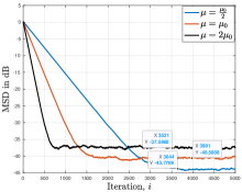
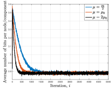
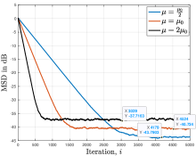
Figure 8: Network performance w.r.t. ${\scriptstyle\mathcal{W}}^{o}$ in (3) for three different values of the step-size ($\mu_{0}=0.003$). In the left and middle plots, the probabilistic ANQ quantizer of Example 2 is employed. (Left) Evolution of the MSD learning curves. (Middle) Evolution of the average number of bits per node, per component, when the variable-rate scheme described in Sec. II-A is used to encode the difference $\boldsymbol{\chi}_{k,i}=\boldsymbol{\psi}_{k,i}-\boldsymbol{\phi}_{k,i-1}$ in (28b). (Right) Evolution of the MSD learning curves when the QSGD quantizer (with $s=2$) of Table I is used.

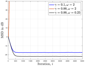
Figure 9: Network performance w.r.t. ${\scriptstyle\mathcal{W}}^{o}$ in (3) for different values of the ANQ quantizer’s parameter $\omega$ and mixing parameter $\gamma$.

References

- [1] R. Nassif, S. Vlaski, M. Antonini, M. Carpentiero, V. Matta, and A. H. Sayed, “Finite bit quantization for decentralized learning under subspace constraints,” in Proc. Eur. Signal Process. Conf., Sep. 2022, pp. 1–5.
- [2] B. McMahan, E. Moore, D. Ramage, S. Hampson, and B. A. Y. Arcas, “Communication-efficient learning of deep networks from decentralized data,” in Proc. Int. Conf. Artif. Intell. Stat., Ft. Lauderdale, FL, USA, 2017, vol. 54, pp. 1273–1282.
- [3] T. Li, A. K. Sahu, A. S. Talwalkar, and V. Smith, “Federated learning: Challenges, methods, and future directions,” IEEE Signal Process. Mag., vol. 37, pp. 50–60, May 2020.
- [4] P. Kairouz, H. B. McMahan, B. Avent, A. Bellet, M. Bennis, A. N. Bhagoji, , and S. Zhao, “Advances and open problems in federated learning,” Found. Trends Mach. Learn., vol. 14, no. 1–2, pp. 1–210, 2021.
- [5] D. Alistarh, D. Grubic, J. Li, R. Tomioka, and M. Vojnovic, “QSGD: Communication-efficient SGD via gradient quantization and encoding,” in Proc. Adv. Neural Inf. Process. Syst., Long Beach, CA, USA, 2017, pp. 1709–1720.
- [6] M. Aledhari, R. Razzak, R. M. Parizi, and F. Saeed, “Federated learning: A survey on enabling technologies, protocols, and applications,” IEEE Access, vol. 8, pp. 140699–140725, Jul. 2020.
- [7] V. Smith, C.-K. Chiang, M. Sanjabi, and A. S. Talwalkar, “Federated multi-task learning,” in Proc. Adv. Neural Inf. Process. Syst., Long Beach, CA, USA, Dec. 2017, vol. 30.
- [8] A. H. Sayed, “Adaptation, learning, and optimization over networks,” Found. Trends Mach. Learn., vol. 7, no. 4-5, pp. 311–801, 2014.
- [9] A. H. Sayed, “Adaptive networks,” Proc. IEEE, vol. 102, no. 4, pp. 460–497, 2014.
- [10] A. H. Sayed, S.-Y. Tu, J. Chen, X. Zhao, and Z. Towfic, “Diffusion strategies for adaptation and learning over networks,” IEEE Signal Process. Mag., vol. 30, no. 3, pp. 155–171, May 2013.
- [11] R. Nassif, S. Vlaski, C. Richard, J. Chen, and A. H. Sayed, “Multitask learning over graphs: An approach for distributed, streaming machine learning,” IEEE Signal Process. Mag., vol. 37, no. 3, pp. 14–25, 2020.
- [12] A. Koloskova, S. Stich, and M. Jaggi, “Decentralized stochastic optimization and gossip algorithms with compressed communication,” in Proc. Int. Conf. Mach. Learn., 2019, vol. 97, pp. 3478–3487.
- [13] A. Nedic and A. Ozdaglar, “Distributed subgradient methods for multi-agent optimization,” IEEE Trans. Automat. Contr., vol. 54, no. 1, pp. 48–61, Jan. 2009.
- [14] D. P. Bertsekas, “A new class of incremental gradient methods for least squares problems,” SIAM J. Optim, vol. 7, no. 4, pp. 913–926, 1997.
- [15] A. G. Dimakis, S. Kar, J. M. F. Moura, M. G. Rabbat, and A. Scaglione, “Gossip algorithms for distributed signal processing,” Proc. IEEE, vol. 98, no. 11, pp. 1847–1864, 2010.
- [16] J. Plata-Chaves, A. Bertrand, M. Moonen, S. Theodoridis, and A. M. Zoubir, “Heterogeneous and multitask wireless sensor networks – Algorithms, applications, and challenges,” IEEE J. Sel. Top. Signal Process., vol. 11, no. 3, pp. 450–465, 2017.
- [17] J. F. C. Mota, J. M. F. Xavier, P. M. Q. Aguiar, and M. Püschel, “Distributed optimization with local domains: Applications in MPC and network flows,” IEEE Trans. Automat. Contr., vol. 60, no. 7, pp. 2004–2009, 2015.
- [18] R. Nassif, C. Richard, A. Ferrari, and A. H. Sayed, “Diffusion LMS for multitask problems with local linear equality constraints,” IEEE Trans. Signal Process., vol. 65, no. 19, pp. 4979–4993, 2017.
- [19] V. Kekatos and G. B. Giannakis, “Distributed robust power system state estimation,” IEEE Trans. Power Syst., vol. 28, no. 2, pp. 1617–1626, 2013.
- [20] S. A. Alghunaim and A. H. Sayed, “Distributed coupled multiagent stochastic optimization,” IEEE Trans. Automat. Contr., vol. 65, no. 1, pp. 175–190, 2020.
- [21] R. Nassif, S. Vlaski, C. Richard, and A. H. Sayed, “Learning over multitask graphs–Part I: Stability analysis,” IEEE Open Journal of Signal Processing, vol. 1, pp. 28–45, 2020.
- [22] A. K. Sahu, D. Jakovetić, and S. Kar, “: A distributed random fields estimator,” IEEE Trans. Signal Process., vol. 66, no. 18, pp. 4980–4995, 2018.
- [23] J. Chen, C. Richard, and A. H. Sayed, “Multitask diffusion adaptation over networks,” IEEE Trans. Signal Process., vol. 62, no. 16, pp. 4129–4144, 2014.
- [24] R. Nassif, S. Vlaski, and A. H. Sayed, “Adaptation and learning over networks under subspace constraints–Part I: Stability analysis,” IEEE Trans. Signal Process., vol. 68, pp. 1346–1360, 2020.
- [25] R. Nassif, S. Vlaski, and A. H. Sayed, “Adaptation and learning over networks under subspace constraints–Part II: Performance analysis,” IEEE Trans. Signal Process., vol. 68, pp. 2948–2962, 2020.
- [26] P. Di Lorenzo, S. Barbarossa, and S. Sardellitti, “Distributed signal processing and optimization based on in-network subspace projections,” IEEE Trans. Signal Process., vol. 68, pp. 2061–2076, 2020.
- [27] A. Nedic, A. Olshevsky, A. Ozdaglar, and J. N. Tsitsiklis, “Distributed subgradient methods and quantization effects,” in Proc. IEEE Conf. Decis. Control, Cancun, Mexico, Dec. 2008, pp. 4177–4184.
- [28] X. Zhao, S.-Y. Tu, and A. H. Sayed, “Diffusion adaptation over networks under imperfect information exchange and non-stationary data,” IEEE Trans. Signal Process., vol. 60, no. 7, pp. 3460–3475, 2012.
- [29] R. Nassif, C. Richard, J. Chen, A. Ferrari, and A. H. Sayed, “Diffusion LMS over multitask networks with noisy links,” in Proc. IEEE Int. Conf. Acoust., Speech, Signal Process., Shanghai, China, 2016, pp. 4583–4587.
- [30] D. Thanou, E. Kokiopoulou, Y. Pu, and P. Frossard, “Distributed average consensus with quantization refinement,” IEEE Trans. Signal Process., vol. 61, no. 1, pp. 194–205, 2013.
- [31] N. Michelusi, G. Scutari, and C.-S. Lee, “Finite-bit quantization for distributed algorithms with linear convergence,” IEEE Trans. Inf. Theory, vol. 68, no. 11, pp. 7254–7280, Nov. 2022.
- [32] M. Carpentiero, V. Matta, and A. H. Sayed, “Distributed adaptive learning under communication constraints,” Available as arXiv:2112.02129, Dec. 2021.
- [33] M. Carpentiero, V. Matta, and A. H. Sayed, “Adaptive diffusion with compressed communication,” in Proc. IEEE Int. Conf. Acoust., Speech, Signal Process, 2022, pp. 1–5.
- [34] D. Kovalev, A. Koloskova, M. Jaggi, P. Richtarik, and S. Stich, “A linearly convergent algorithm for decentralized optimization: Sending less bits for free!,” in Proc. Int. Conf. Artif. Intell. Stat., Virtual, 2021, pp. 4087–4095.
- [35] N. Singh, D. Data, J. George, and S. Diggavi, “SPARQ-SGD: Event-triggered and compressed communication in decentralized optimization,” IEEE Trans. Automat. Contr., vol. 68, no. 2, pp. 721–736, 2023.
- [36] N. Singh, D. Data, J. George, and S. Diggavi, “SQuARM-SGD: Communication-efficient momentum SGD for decentralized optimization,” in Proc. IEEE Int. Symp. Inf. Theory, Melbourne, Victoria, Australia, 2021, pp. 1212–1217.
- [37] H. Tang, S. Gan, C. Zhang, T. Zhang, and J. Liu, “Communication compression for decentralized training,” in Proc. Adv. Neural Inf. Process. Syst., Montréal, Canada, 2018, pp. 7663–7673.
- [38] H. Taheri, A. Mokhtari, H. Hassani, and R. Pedarsani, “Quantized decentralized stochastic learning over directed graphs,” in Proc. Int. Conf. Mach. Learn., Jul. 2020, vol. 119, pp. 9324–9333.
- [39] X. Zhang, J. Liu, Z. Zhu, and E. S. Bentley, “Compressed distributed gradient descent: Communication-efficient consensus over networks,” in Proc. IEEE Int. Conf. Commun., Paris, France, 2018, pp. 2431–2439.
- [40] A. Reisizadeh, A. Mokhtari, H. Hassani, and R. Pedarsani, “An exact quantized decentralized gradient descent algorithm,” IEEE Trans. Signal Process., vol. 67, no. 19, pp. 4934–4947, 2019.
- [41] A. Gersho and R. M. Gray, Scalar Quantization I: Structure and Performance, pp. 133–172, Springer US, Boston, MA, 1992.
- [42] T. C. Aysal, M. J. Coates, and M. G. Rabbat, “Distributed average consensus with dithered quantization,” IEEE Trans. Signal Process., vol. 56, no. 10, pp. 4905–4918, 2008.
- [43] L. M. Nguyen, P. H. Nguyen, M. Van Dijk, P. Richtárik, K. Scheinberg, and M. Takáč, “SGD and Hogwild! Convergence without the bounded gradients assumption,” in Proc. Int. Conf. Mach. Learn., Stockholm, SWE, 2018.
- [44] B. T. Polyak, Introduction to Optimization, Optimization Software, New York, 1987.
- [45] R. Nassif, S. Vlaski, and A. H. Sayed, “Distributed inference over networks under subspace constraints,” in Proc. IEEE Int. Conf. Acoust., Speech, Signal Process, Brighton, UK, 2019, pp. 5232–5236.
- [46] H. Gish and J. Pierce, “Asymptotically efficient quantizing,” IEEE Trans. Inf. Theory, vol. 14, no. 5, pp. 676–683, 1968.