How Far Does the Predictive Decision Impact the Software Project? The Cost, Service Time, and Failure Analysis from a Cross-Project Defect Prediction Model

Abstract

Context: Cross-project defect prediction (CPDP) models are being developed to optimize the testing resources.
Objectives: Proposing an ensemble classification framework for CPDP as many existing models are lacking with better performances and analysing the main objectives of CPDP from the outcomes of the proposed classification framework.
Method: For the classification task, we propose a bootstrap aggregation based hybrid-inducer ensemble learning (HIEL) technique that uses probabilistic weighted majority voting (PWMV) strategy. To know the impact of HIEL on the software project, we propose three project-specific performance measures such as percent of perfect cleans (PPC), percent of non-perfect cleans (PNPC), and false omission rate (FOR) from the predictions to calculate the amount of saved cost, remaining service time, and percent of the failures in the target project.
Results: On many target projects from PROMISE, NASA, and AEEEM repositories, the proposed model outperformed recent works such as TDS, TCA+, HYDRA, TPTL, and CODEP in terms of F-measure. In terms of AUC, the TCA+ and HYDRA models stand as strong competitors to the HIEL model.
Conclusion: For better predictions, we recommend ensemble learning approaches for the CPDP models. And, to estimate the benefits from the CPDP models, we recommend the above project-specific performance measures.

1 Introduction

Building reliable software is the ultimate goal for the project management team [1]. Due to the enormous increase in building large-scale complex software systems, with the limited available resources such as manpower and cost, achieving the project goals within the deadlines is a challenging task [2, 3]. In addition to that, the test team has to put more effort into achieving the correct behaviour of the developed software by removing/modifying the defective modules. To mitigate such challenges, automation tools such as software defect prediction (SDP) models are being developed [4, 5, 6]. The motivation behind building SDP models is that it reduces the workload on the test team by reducing the testing time of software modules and, consequently, it reduces the total project’s budget [7, 8].

Because of such advantages, research on building SDP models is attracted by both academia and the software industry. The main objective of SDP models is to predict the defect proneness of a module in newly developed software. These SDP models are being built based on machine learning (ML) algorithms that use metric suits as the independent variables (features). Later, using the trained SDP models, a newly developed module is classified into either defective or clean classes.

Recent studies have introduced two major categories of SDP, such as with-in project defect prediction (WPDP) and cross-project defect prediction (CPDP). The WPDP models utilise the module information from the released versions of a project to train the prediction model. The defect proneness of the modules in a currently developing version of that project is then found using the trained WPDP model [9, 10, 6]. Lack of sufficient defect data is the major constraint in developing WPDP models [11]. To overcome the problem of insufficient data, the CPDP models utilise the defect data of the various released projects (and their releases) to train the ML model.

Finding the defect proneness of the modules in a cross-project domain is a challenging task because, training a model on the developed project(s) may not be generalisable well on the target project [12]. For this, many transfer learning approaches were proposed in order to provide solution by transferring the common knowledge from source project(s) to the target projects [13, 14, 15, 16, 17]. In addition, ensemble learning models have also been proposed in the literature [18, 12] since these models provide solutions based on the group of classifiers rather than utilising single classifiers. However, Herbold et al [19] claim that none of the proposed approaches in the literature consistently achieve significant results.

To mitigate the risk of poor classification, in this work, we propose a hybrid-inducer ensemble learning (HIEL) technique based on the bootstrap aggregation methodology. This classification framework is constructed based on a diversity generation mechanism. The advantage of using the diversity generation mechanism is that it better captures the generalisable properties of the test instances across the different domains by relaying on the group of classifiers where, the solution is achieved based on the average of the predicted outcomes [20]. Hence, instead of utilising one classifier, HIEL utilises a group of various inducers such as Logistic Regression (LR), Support Vector Machine (SVM), Decision Trees (DT), Nav̈e Bayes (NB), k-Nearest Neighbours (k-NN), and Artificial Neural Network (NN), during the training phase. Here, each inducer takes a random sample from the original training set, which is collected from the augmented source projects and builds the ensemble of classifiers. Later, the predictions of each classifier are fed as input to the combiner model called the probabilistic weighted majority voting (PWMV) approach to observe the final decision. The PWMV works on the basis of a weighted majority voting approach where, at each trial, the weights are updated based on the parameter $\beta$. In this process, whenever the expert (classifier) makes a mistake on the test example, gets penalised weight. Here, the weights are assigned to the experts as probabilities. Similarly, if the expert makes the correct decision, then that expert will be considered as the most probable expert in the near future. In this way, the PWMV predicts the class label for the test instance. The detailed working procedure of the proposed HIEL model using PWMV is given in Section 3.

To find the superiority of the proposed HIEL approach, this work includes a comparison of recent implementations such as Transfer Component Analysis Plus (TCA+) [15], Training Data Selection (TDS) [21], HYbrid moDel Reconstruction Approach (HYDRA) [12], COmbined DEfect Predictor (CODEP) [18], and Two-Phase Transfer Learning (TPTL) [22] models. For the empirical analysis, we have used 38 releases of 12 software projects from the publicly available PROMISE repository [23], 12 releases of 6 projects from the NASA MDP repository [24], and 5 projects from the AEEEM repository [25]. The results show that the proposed HIEL model with PWMV outperforms the above models on the majority of the target projects and is a strong competitor to the HYDRA model. The detailed discussion of the performance of the HIEL using PWMV is given in Section 5.

In addition to proposing a classification model, there is a need to analyse the impact of the prediction result that shows on the project attributes such as the amount of saved budget, the percent of remaining service time, and the percent of failures that may occur in a software with the introduction of the CPDP model in the real-time scenario. Making use of these measures is essential because this is the true goal of SDP research. To the best of our knowledge, this work is intended to provide such an analysis of the proposed CPDP model, as such analysis was not provided in the literature.

For this objective, we have proposed three prediction project-specific performance measures such as Percent of Perfect Cleans (PPC), Percent of Non-Perfect Cleans (PNPC), and False Omission Rate (FOR). The PPC measure is used to analyse the total savings in the total allocated budget in the developing project, where as PNPC is used to estimate the amount of time required to service (based on the remaining number of code edits) the code. The measure-FOR calculates the percent of failures that may occur in the software, after deploying the project. The experimental results show that, the projects from the repositories such as PROMISE, NASA, and AEEEM have 49.70%, 68.70%, and 58.98% of budget savings, respectively. In this regard, the testers have to put their efforts on the code for only 50.30%, 31.30%, and 41.02% of the total time to remove the total defect content (including the observed failures) in the projects of PROMISE, NASA, and AEEEM, respectively. We hope this experiment will pave the path for future CPDP (in general, the SDP) research to more focus on developing the prediction models that provide analysis on the benefits of the project from the predictions.

With this work, we have made the following principal contributions to the cross-project defect prediction study:

1. Proposed a novel hybrid-inducer ensemble learning (HIEL) technique that uses bagging methodology to train the CPDP model. For this, a combiner approach called probabilistic weighted majority voting (PWMV) is employed to mitigate the risk of poor classification and to achieve the generalisable properties of defective instances that work across the target projects.

2. Provided a tight upper bound on the number of mistakes made by the best expert (classifier) in the PWMV combiner approach.

3. Proposed three project specific measures such as the amount of saved budget, amount of remaining service time for the tester, and the percent of failures that may occur in the project. To the best of our knowledge, estimating such project-specific measures from the predictions is new to this SDP (in any sub-category) task.

Paper Organization: Section 2 presents the literature review on classification models developed for CPDP. In section 3, the proposed method for training is presented along with the PWMV combiner approach. The elements required to develop and evaluate the proposed model are given in Section 4. This section also defines the project-specific performance measures. The results of the proposed model and the detailed discussion are presented in section 5. Threats to the validity of the proposed work are presented in section 6. Section 7 concludes the work and discusses the future work.

2 Background and Related Work

Section 2.1 reviews the classification models for CPDP. Section 2.2 discusses the current status of the literature on using ensemble models for CPDP. Section 2.3 discusses the different strategies of generating diverse classifiers in the ensemble learning methodology.

2.1 Cross Project Defect Prediction Studies

Predicting the defect proneness of the source-code components is still evolving, and proposing a successful prediction model is still a challenging task [19].

As discussed in section 1, the CPDP models are majorly suffering from the data distribution among the source and target projects. As a consequence, these models are yielding poor predictive performance. To conquer the challenge of data distribution among source and target projects, many transfer learning models have been proposed [14, 15, 21, 22] in the literature.

In [14], Ying Ma et al. proposed a Transfer Naïve Bayes (TNB) for the CPDP task. They exploited the sample weighting algorithm on the data across all the source projects to form a training dataset. From the experimentation on NASA and SOFTLAB datasets, they concluded that, when there is not enough training data to train a strong classifier, knowledge acquired from various source projects based on the feature-level information may help to obtain better performances. For the same problem, in [15], Nam et al. proposed a transfer component analysis plus (TCA+) model based on their prior work called transfer component analysis (TCA) [26]. The TCA tries to find the latent feature space between source and target projects by minimising the data distributions. From the experimentation on PROMISE projects, they observed the improved accuracy of the target projects upon selecting a suitable source project.

On the similar problem, Herbold in [21] proposed two distance based similarity measures to select the training data across the source projects. To form the training dataset, k-nearest neighbour algorithm was employed. From the experimental evaluation of TDS on the PROMISE projects, they concluded that improved performance can be obtained through selecting appropriate training data. In [27], Zhou Xu et al. proposed a method called balanced distribution adaptation (BDA), targeted to show the impact of conditional distribution differences in selecting the source and target data.

Recently, Liu et al. in [22] proposed a two-phase transfer learning (TPTL) model to overcome the problem that is posed by the TCA+ model. That is, the performance of TCA+ may vary on various target projects based on the selection of different source projects. For this, they proposed the TPTL model that works in two phases. In the first phase, a source project estimator (SPE) was proposed to select any two source projects for the target project where the two source projects form the highest distribution similarity. Later, TCA+ was employed to build two classification models on the selected source projects. TPTL demonstrated improved performance on the PROMISE projects when compared to state-of-the-art models.

Selecting the appropriate simplified metric suits may also impact the performance of the defect prediction models. A detailed empirical analysis was presented in [28] by Peng He et al. that discussed the practical recommendations for selecting the training data, subset of metrics, and classification models. Hosseini et al. in [29], also aimed to demonstrate the use of different feature sets for successful performances.

However, achieving generalised predictive performance across the target projects is still a challenging task [12, 20]. This is because the use of specific classifiers is causing such low classification performances [20]. To mitigate such challenges, recently, ensemble learning models have been proposed [18, 16, 30, 12] to overcome the poor predictive performances that these models are exhibiting on some target projects.

2.2 Ensemble Learning Approaches for CPDP

In contrast to discussing the distributional characteristics of the data, proposing ensemble learning models has emerged as a tool for CPDP in recent years. In [18], Panichella et al. proposed a CODEP (COmbined DEfect Predictor) approach that combines the outputs of six classifiers. Their research suggests using ensemble models for CPDP problems because many base-line classifiers perform poorly. Zhang et al. in [16] also suggested the benefits of utilising the ensemble frameworks for the CPDP problem. In [30], Laradji et al. targeted to show the benefits of combining feature selection and ensemble learning. Their approach concluded that using fewer features with ensemble learning can help to mitigate issues like data imbalance and feature redundancy.

An extensive empirical study was conducted by Xin Xia et al in [12] to address the CPDP problem. Their approach (HYbrid moDel Reconstruction Approach (HYDRA)) is a combination of genetic algorithm and AdaBoost ensemble learning methodology, to create a bag of classifiers. This experiment makes use of an enormous number of classifiers in the process of obtaining the final decision. The HYDRA model consists of two steps: model building step and prediction step. Similar to our work, they have taken the common metrics from the source projects data and target projects data, to build the classification model. The model building step is used to generate the numerous classifiers. The model building step contains two phases such as genetic algorithm (GA) phase and ensemble learning (EL) phase. In the GA phase, for each source project, and training target data (which is the 5% of the labeled target data), they build a classifier, and in total they build N+1 classifiers (assuming there are N number of source projects). Here, the extra one classifier is built on the training target data alone. Next, HYDRA uses GA to search for the best composition of these classifiers. In the EL phase, they built multiple GA classifiers, by running the GA phase multiple times (k times), and composing these GA classifiers according to their training error rate. In the prediction step, a new unlabeled instance from the target data will be given as input to the HYDRA model to observe the prediction. This experiment indicates the use of an enormous number of classifiers in the process of obtaining a better final decision.

However, a survey in [19] by Herbold et al. indicates the requirement of proposing a better classification model for this application. To alleviate unstable classification performances, Breiman and Polikar in [31] and [20], respectively, suggest using an ensemble of diverse classifiers in the decision making process. In addition, their study reveals several interesting conclusions, such as: 1) the ensemble of diverse classifiers can address the instability of the individual weak learners; 2) it can provide a generalisable solution for the classification task. Hence, our study targeted to implement the diversity generation mechanism as the classification technique to approach the CPDP problem.

2.3 Diversity Generation Mechanism

Ensemble learning methods draw near-accurate final decision for a test example on the basis of utilising a huge number of diverse classifiers. According to the definition of ensemble learning, as the number of diverse classifiers increases infinitely, then the probability of correct decision on the test example approaches 1 [31, 20]. Hence, to obtain the most accurate prediction, it is required to generate as many diverse classifiers as possible.

In order to increase the number of decision makers, different diversity generation strategies such as manipulating the training sample, feature subspace sampling, inclusion of hybrid inducer models, parameter optimization, and changing the output representation are utilised [32]. Note that, usage of such components of taxonomy may not be mutually exclusive. That is, according to the applicability, one or more strategies can be combined to generate the diverse classifiers.

By considering the training time of an ensemble classifier, we make use of two diverse generation strategies, such as sampling with replacement on the original training data and hybrid-inducer strategies, to generate the diverse classifiers. The strategies in the construction of the proposed ensemble learning methodology is given below.

2.3.1 The Hybrid-Inducer System

In the hybrid inducer strategy, multiple base inducers are used to generate the diversity in the ensemble approach. Note that, a classification algorithm is also referred to as an inducer and an instance of an inducer for a set of training data is called a classifier. Ideally, this hybrid-inducer strategy would always perform as well as the best of its ingredients. The advantage of this strategy is that, it can solve the dilemma which arises from the famous “no free lunch theorem”. This theorem implies that a certain inducer is considered successful only insofar as its bias matches with the characteristics of the application domain [33]. Therefore, for a given machine learning application, the practitioner needs to decide which inducer needs to be used. But the hybrid-inducer strategy obviates the need to try each one and simplifies the entire process. That is, using the hybrid-inducer strategy, each inducer obtains a bias (either explicit or implicit) that causes it to prefer some generalisations over others. Hence, this hybrid inducer strategy always performs better among the other strategies [32]. To generate numerous diverse classifiers, in this work, we use six base inducers such as LR, k-NN, NB, SVM, NN, and DT. The description of these inducers is discussed in section 4.2.

2.3.2 The Bootstrapping

This is the general approach to create a bag of classifiers. Using this strategy, each inducer is trained using a different variation, subset, or sample of the original training set. This strategy is effective for the inducer, which has a relatively large variance-error. That is, a small variation in the training set may cause a major change in the performance of the utilised classifier. In this approach, the training samples are generated (from the original training set) majorly using either with replacement or with-out replacement strategies. If the training set contain massive data-points, training the classifier become a bottleneck. Hence, in that case, the common strategy is to partition the entire population (original training data) into disjoint sets and train a classifier on each partitioned data [32]. If the original training set contain a limited data-points, then the common approach is to sample the training set with the replacement. In this work, we sample the original set of population data (source projects data) with replacement as many source projects contain a few data-points. To ensure a sufficient number of training instances in each of the drawn sample, it is a common practice to set the size of the sample as the size of the original training set [32].

The ensemble of classifiers is generated based on the parameter called sample number. A classifier is generated for each sample based on the utilised inducer. To select the value of the sample number, we followed the result of a study by Opitz in [34]. The study suggests using 10 samples to generate diverse classifiers to achieve better predictions on the test data. This sample number is treated as the stopping criterion in generating the diverse classifiers.

3 The Hybrid-Inducer Ensemble Learning (HIEL) Technique

The first part of this section presents the proposed diversity generation mechanism, and the second part of this section presents the combiner scheme called probabilistic weighted majority voting (PWMV).

3.1 Training the HIEL Model

The training procedure of the HIEL model is given in the algorithm 1. The prerequisites for this model are: training data (source project’s information), test data (target project’s data), inducers, and a constant to form the bootstrap samples. Before training the HIEL model, training data $\mathcal{S}$ is collected by augmenting all the source projects’ (including their releases) data. Based on the assumption that each project is developed in similar environments, by matching the metrics in each project, we augment the module’s information across all the source projects. Here, each metric is treated as an independent variable in training the model. Similarly, we prepare the test data (validation set) $\mathcal{V}$ from the target project to find the defect proneness of the newly developed modules. Later, to generate an ensemble of diverse classifiers, two diversity generation schemes, such as hybrid inducer system, and bootstrap aggregation, are used, and the description of these methods is given in the section 2.3.

As discussed in section 2.3, HIEL model employs sampling with replacement to collect the training data $\mathcal{S}_{t}^{j}$ of size k from the original training set $\mathcal{S}$. Hence, after sampling with replacement, the module’s information is included in the sample at-least zero times.

The algorithm 1 iterates over |$\mathcal{I}$| inducers and, for each inducer, T classifiers are generated based on the bootstrap samples. That is, in $t^{th}$ iteration $t\in\{1,2\dots,T\}$, a random sample $\mathcal{S}_{t}^{j}$ $j\in\{1,2\dots,|\mathcal{I}|\}$ of size k, k=$|\mathcal{S}|$, is drawn with the replacement from $\mathcal{S}$. Now, each inducer $\mathcal{I}_{j}$ takes the drawn sample $\mathcal{S}_{t}^{j}$ and builds a classifier $\mathcal{C}_{j}[t]$ in $t^{th}$ iteration. Then, using $\mathcal{C}_{j}[t]$, predict the class labels for the test examples in a set $\mathcal{V}$ into defect (1) or clean (0), and store the predicted class labels in $\mathcal{P}_{j}[t]$. Since, the algorithm takes |$\mathcal{I}$| inducers and T samples for each inducer, as a result, after completion of all the iterations, a total of |$\mathcal{I}|\times$T classifiers were built. In the end, the predicted class labels $\mathcal{P}_{j}[t]$, are given as input to the probabilistic weighted majority voting combiner model to get the final prediction for the test examples $\mathcal{V}$. The figure 1 represents the proposed training framework of the HIEL model and, the classification procedure using PWMV.

1

Input: Inducers $\mathcal{I}$ = {$\mathcal{I}_{1}$, $\mathcal{I}_{2}$, $\cdots$, $\mathcal{I}_{i}$},

Training set size k = $|\mathcal{S}|$,

Number of iterations = T = 10

Output: Classifiers, $\mathcal{C}$ = {$\mathcal{C}_{j}[t],j\in\{1,2,\dots,i\},t\in\{1,2,\dots,T\}$}

Predictions, $\mathcal{P}$ = {$\mathcal{P}_{j}[t],j\in\{1,2,\dots,i\},t\in\{1,2,\dots,T\}$}

Data: Population Data $\mathcal{P}d$ = Training Set ($\mathcal{S}$) $\cup$ Validation Set ($\mathcal{V}$),

Training Set $\mathcal{S}$ = {Defects data collected from source projects},

Validation Set $\mathcal{V}$ = {Defects data of the target project}

2 Function HIEL($\mathcal{P}d$, $\mathcal{S}$, $\mathcal{V}$, $\mathcal{I}$, T, k):

3       j = 1;

4       while j $\leq|\mathcal{I}|$ do

5             t = 1;

6             while t $\leq$ N do

7                   $\mathcal{S}_{t}^{j}$ = Sample $\mathcal{S}$ with k observations randomly with replacement;

8                   $\mathcal{Y}_{t}^{j}$ = Class labels of test set $\mathcal{V}$;

9                   $\mathcal{C}_{j}[t]$ = Build classifier using $\mathcal{I}_{j}$ on $\mathcal{S}_{t}^{j}$;

10                   $\mathcal{P}_{j}[t]$ = Predict the class labels into defect or clean for test set $\mathcal{V}$ using the classifier $\mathcal{C}_{j}[t]$;

11                   t++;

12                  

13             end while

14            j++;

15            

16       end while

17      

18 return $\mathcal{P}$

Algorithm 1 HIEL-Diversity Generation Phase

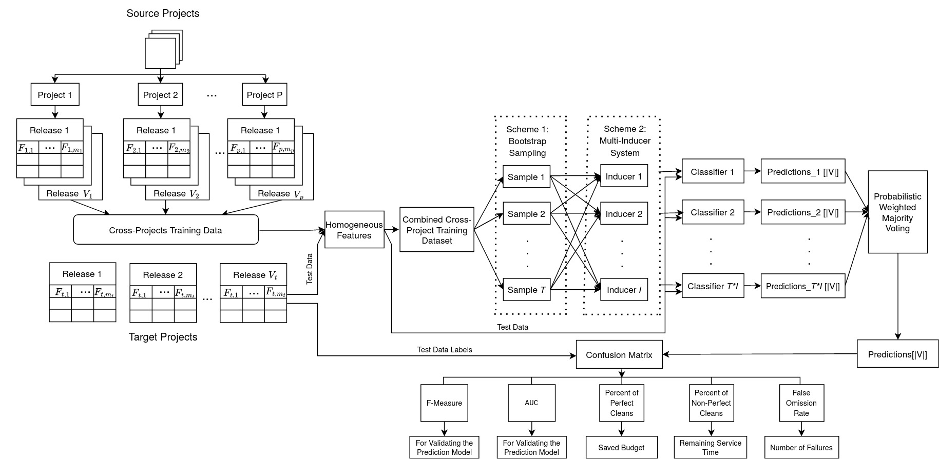
Figure 1: Work flow of the classification procedure using proposed HIEL method

3.2 Probabilistic Weighted Majority Voting for Classification

After obtaining the predictions from the HIEL model on the test data, the combiner method called probabilistic weighted majority voting (PWMV) is employed to predict the final class label for the test instance. The intuition behind the PWMV combiner method is developed based on the weighted majority voting (WMV) strategy [20]. The weighted majority voting algorithm maintains a list of weights (let us assume the weights as, $w_{1},w_{2},\cdots,w_{n}$), for a set of $n$ experts, and computes the final prediction based on the weighted majority of the expert opinions. Without loss of generality, where each single expert is assumed as a trained classifier. Now, in WMV, uniform weights are distributed among all the experts. For simplicity, let the weight given to all the experts be considered to be 1. Given a sequence of experts (classifiers), at each test example, if the expert makes the wrong prediction, gets the punishment of half of its weight. Now, to classify the text example, add the weights of all the experts in the two categories (defective (1) or clean (0)), and compare the resulting weights of these two categories; then, classify the test example to the class with the highest weight.

According to Blum [35], the regular WMV method guarantees an upper bound of $2.14(\log_{2}n+\epsilon)$ mistakes during several trials. Where, $\epsilon$ is the number of mistakes made by the best expert, so far, and n is the total number of experts involved in the final decision. This (the upper bound, $2.14(\log_{2}n+\epsilon)$) is still problematic because, the best expert still makes the mistakes of more than 20% of the total trials. As this (depending on $\epsilon$) is the limitation on achieving better results, in this case, a probabilistic version of the weighted majority voting is used to reduce the upper bound on the total mistakes made by the best expert [35]. Here, in probabilistic weighted majority voting (PWMV), the weights of individual experts are updated using the parameter $\beta,0<\beta<1$. Where $\beta$ is the amount of penalty that is given to each mistaken expert in the process of making the decision. The intuition behind the PWMV algorithm is that this dilutes (reduces) the worst possible mistakes made by the best expert. This is because, instead of considering the weights as probabilities, each outcome for the test example is predicted with a probability proportionate to its weight. That is, as the weight of the expert reduces, then the probability of the expert predicting the class label also reduces. The general algorithmic procedure to classify new instances using PWMV is given in the algorithm 2.

1Initialize the weights of all the experts $w=\{w_{11},\cdots,w_{1T},w_{21},\cdots,w_{2T},{\cdots,}w_{|\mathcal{I}|1},\cdots,w_{|\mathcal{I}|T}\}$ to 1;

2 Observe the predictions from all the experts $\hat{y}=\{\hat{y}_{11},\hat{y}_{12},\cdots,\hat{y}_{|\mathcal{I}|T}\}$ for the test example $x_{i}$;

3 Initialize $\beta$;

4 Calculate W = $\sum_{i=1}^{|\mathcal{I}|}\sum_{j=1}^{T}w_{ij}$;

5 while Test Set is not Empty do

6       for All the experts $\{c_{1},c_{2},\cdots,c_{|\mathcal{I}|T}{\}}$ do

7             if The prediction $\hat{y_{i}}$ matches with the actual value,$y_{i}$ then

8                   Predict the class label for $x_{i}$ as $\hat{y_{i}}$ with the maximum probability $\frac{w_{i}}{W}$;

9                   Do not modify the weight of the expert $c_{i}$;

10                  

11            else

12                   Penalise mistaken expert by multiplying its weight with $\beta$. (That is $w_{i}=w_{i}*\beta$);

13                   Update the probability of the expert with $\frac{w_{i}}{W}$ ;

14                  

15             end if

16            

17       end for

18      Update the weight value W with the resulting weights ($W=\sum_{i}w_{i}$);

19      

20 end while

Algorithm 2 Probabilistic Weighted Majority Voting Algorithm

Using the analysis on minimising the upper bound on the total mistakes made by the best expert [35], the following corollary defines the maximum upper bound on the total mistakes made by the best expert using PWMV.

Corollary 1.

Given the weights $w=\{w_{11},w_{12},\cdots,w_{1T},\\ w_{21},w_{22},\cdots,w_{2T},{\cdots,}w_{|\mathcal{I}|1},w_{|\mathcal{I}|2},\cdots,w_{|\mathcal{I}|T}\}$ of experts and the set of predictions $\hat{y}=\{\hat{y}_{11},\hat{y}_{12},\cdots,\hat{y}_{|\mathcal{I}|T}\}$ on the test instance, ${x}_{l}$, the upper bound on the number of mistakes $\mathrm{M}$ made by the PWMV satisfies:

$$\mathrm{M}\leq\frac{\log|\mathcal{I}|+\log T-\epsilon*\log\beta}{1-\beta}$$

Where $|\mathcal{I}|$ is the expert index, $\beta$ is the penalty given to each mistaken expert and $\epsilon$ is the number of mistakes so far made by the best expert chosen for the HIEL model.

Proof.

Assign the weights of each expert $w=\{w_{11},w_{12},\cdots,\\ w_{1T},w_{21},w_{22},\cdots,w_{2T},{\cdots,}w_{|\mathcal{I}|1},w_{|\mathcal{I}|2},\cdots,w_{|\mathcal{I}|T}\}$ to 1. Observe the predictions $\hat{y}=\{\hat{y}_{11},\hat{y}_{12},\cdots,\hat{y}_{|\mathcal{I}|T}\}$ from all the hybrid experts on ${x}_{l}$. From the weights w, calculate;

$$W=\sum_{i=1}^{|\mathcal{I}|}\sum_{j=1}^{T}w_{ij}.$$ (1)

Let $F_{i}$ is the total weight on the wrong answers on the $i^{th}$ trial. Suppose, t trials have been experienced. And, let $\mathrm{M}$ be the expected number of mistakes made so far. It is defined as $\mathrm{M}$ = $\sum_{i=1}^{t}F_{i}$.

On the $i^{th}$ example, the updated weight $W^{{}^{\prime}}$ is observed as:

$$W^{\prime}=W*(1-(1-\beta)F_{i})$$ (2)

Where $\beta$ is the penalty given to the each mistaken expert. Now, similarly, for all the experts from HIEL, the updated final weight is observed as:

$$W^{\prime}=|\mathcal{I}|*T*\prod_{i=1}^{t}(1-(1-\beta)F_{i})$$ (3)

Now, let $\epsilon$ be the number of mistakes made by the best expert so far. Again, using the fact that, $W^{{}^{\prime}}$ is as large as the weight of the best expert, then we have:

$$|\mathcal{I}|*T*\prod_{i=1}^{t}(1-(1-\beta)F_{i})\geq\beta^{\epsilon}$$ (4)

Apply log on both sides, then;

$$\log(|\mathcal{I}|*T)+\sum_{i=1}^{t}\log(1-(1-\beta)F_{i})\geq\epsilon\log\beta$$ (5)

$$\implies\epsilon\log(\frac{1}{\beta})\geq-\log(|\mathcal{I}|*T)-\sum_{i=1}^{t}\log(1-(1-\beta)F_{i})$$ (6)

We know, $\log(1-x)=-x-\frac{x^{2}}{2}-\frac{x^{3}}{3}-\cdots$

$\therefore\log(1-x)\leq-x,\forall x$.

Then,

$$\implies\epsilon\log(\frac{1}{\beta})\geq-\log(|\mathcal{I}|*T)+(1-\beta)\sum_{i=1}^{t}F_{i}$$ (7)

$$\implies\epsilon\log(\frac{1}{\beta})\geq-(\log|\mathcal{I}|+\log T)+(1-\beta)*M$$ (8)

where, $\mathrm{M}$ = $\sum_{i=1}^{t}F_{i}$.

$$\implies(1-\beta)*M\leq\epsilon\log(\frac{1}{\beta})+\log|\mathcal{I}|+\log T$$ (9)

$$\implies M\leq\frac{\epsilon\log(\frac{1}{\beta})+\log|\mathcal{I}|+\log T}{(1-\beta)}$$ (10)

This satisfies the above corollary. ∎

4 Empirical Setup

The description of the used defect datasets is presented in Section 4.1. The default parameter setting for the used base-line inducers is provided in Section 4.2. The model specific performance evaluation measures are discussed in Section 4.3. In addition to that, section 4.4 discusses the well known significance tests such as one-sample Wilcoxon signed rank test and Cliff’s delta effect size test.

4.1 Defect Datasets

To construct and validate the prediction model, this work utilises publicly available defect datasets from the repositories such as PROMISE [23], NASA Metrics Data Program (MDP) [24] and AEEEM [25]. For this empirical analysis, we have used a total of 38, 12 and 5 projects from the PROMISE, NASA, and AEEEM repositories, respectively. Where, each PROMISE project is having 24 metrics (features) to represent the software module. For the NASA projects, we have selected 21 common metrics since each project differs with respect to the variable number of metrics. Similarly, for the AEEEM projects, we have used 17 metrics to build the model. Amongst the available set of metrics, the variables that indicate the severity level of the software module are excluded from the AEEEM projects. The description of each project (and its releases), such as the number of modules present in that released version, the total lines of code in the project, the number of defects and the percent of defects in the released version are presented in the table 1.

For the source projects, we have augmented the defect data of all the projects except all releases of the target project. In this regard, each release of the target project is treated as the test data.

Table 1: An overview of utilised projects

Project	Modules	LoC	Defects	%Defects	Project	Modules	LoC	Defects	%Defects
PROMISE Projects
Ant-1.3	125	37,699	20	16.00	Lucene-2.4	340	102,859	203	59.71
Ant-1.4	178	54,195	40	22.47	Poi-1.5	237	55,428	141	59.49
Ant-1.5	293	87,047	32	10.92	Poi-2.0	314	93,171	37	11.78
Ant-1.6	351	113,246	92	26.21	Poi-2.5	385	119,731	248	64.42
Ant-1.7	745	208,653	166	22.28	Poi-3.0	442	129,327	281	63.57
Camel-1.0	339	33,721	13	03.83	Redaktor	176	59,280	27	15.35
Camel-1.2	608	66,302	216	35.53	Synapse-1.0	157	28,806	16	10.19
Camel-1.4	872	98,080	145	16.63	Synapse-1.1	222	42,302	60	27.03
Camel-1.6	965	113,055	188	19.48	Synapse-1.2	256	53,500	86	33.59
Jedit-3.2	272	128,883	90	33.09	Tomcat	858	300,674	77	08.97
Jedit-4.0	306	144,803	75	24.51	Velocity-1.4	196	51,713	147	75.00
Jedit-4.1	312	153,087	79	25.32	Velocity-1.6	229	57,012	78	34.06
Jedit-4.2	367	170,683	48	13.08	Xalan-2.4	723	225,088	110	15.21
Jedit-4.3	492	202,363	11	02.24	Xalan-2.5	803	304,864	387	48.19
Log4j-1.0	135	21,549	34	25.19	Xalan-2.6	885	411,737	411	46.44
Log4j-1.1	109	19,938	37	33.95	Xalan-2.7	909	428,555	898	98.79
Log4j-1.2	205	38,191	189	92.20	Xerces-1.2	440	159,254	71	16.14
Lucene-2.0	195	50,596	91	46.67	Xerces-1.3	453	167,095	69	15.23
Lucene-2.2	247	63,571	144	58.3	Xerces-1.4	588	141,180	437	74.32
NASA Projects
CM1	344	15,486	42	12.21	MW1	264	6,905	27	10.23
JM1	9,953	376,794	1,759	18.24	PC1	759	23,020	61	08.04
KC1	2,096	42,706	325	15.51	PC2	1,585	17,834	16	01.01
KC3	200	6,399	36	18.00	PC3	1,125	33,016	140	12.44
MC1	9,277	66,583	68	00.73	PC4	1,399	30,055	178	12.72
MC2	127	5,503	44	34.65	PC5	17,186	161,695	516	03.01
AEEEM Projects
Eclipse	997	363,633	206	20.66	Mylyn	1,862	135,334	245	13.16
Equinox	324	40,250	129	39.82	PDE	1,497	123,017	209	16.96
Lucene	691	43,732	64	09.26

4.2 Benchmark Machine Learning Classifiers

The proposed HIEL model uses six base inducers such as logistic regression, k-nearest neighbours, support vector machine, Naïve Bayes, neural networks, and decision trees in the training phase.

In the logistic regression (LR) model, a logit model is used to form a relation between the metric suits and the defect attribute. In the case of k-nearest neighbour (k-NN) model, the value of k is chosen based on 10-fold cross validation. As a result, after validating the model with different values of k, we have taken the value of k as 11. For the support vector machine (SVM) model, we have used a linear kernel to train the model. In the case of Naïve Bayes (NB), to avoid the zero-probability problem, we set the Laplace smoothing parameter ($alpha$) to 1 [36]. For the Neural Networks (NN) model, we have used a 2-hidden layered resilient backpropagation algorithm with the weight backtracking mechanism. For the stopping criteria, a 0.5 threshold is used in the partial derivatives of the error function. Later, we have limited the maximum steps in the training model to the value of 1e+5. In the case of decision trees, a general implementation of a classification and regression tree model [37] is employed in this approach.

4.3 Evaluation Measures

Table 2: The confusion matrix represents the actual and predicted defect labels of the target project modules

		Actual values
		Defective	Clean
Predicted values	Defective	TP	FP
	Clean	FN	TN

Performance measures are the key attributes for analysing the benefits of the prediction model. Because the CPDP (in general, the SDP) models are designed to optimise the testing resources, providing benefits from the predictions that are understandable to the project manager is essential and has been ignored in defect prediction studies. For this, in this work, three prediction model specific performance measures such as Percent of Perfect Cleans (PPC), Percent of Non-Perfect Cleans (PNPC) and False Omission Rate (FOR) are introduced for the first time in the SDP (in this case, CPDP) problem context. The measures PPC, PNPC, and FOR are calculated to estimate the saved amount of budget from the total allocated budget, to estimate the remaining service time, and to estimate the percent of failures, respectively,in the developing project. In addition to the above measures, we have used other performance measures such as AUC and F-measure for the comparative analysis.

Similar to the traditional measures, the proposed performance measures are also calculated based on the confusion matrix. The confusion matrix for this binary classification is defined based on the number of actual and predicted values of the test-set instances. In table 2, the number of true positives (TP) represents the number of defective modules which are predicted into its correct class, the number of true negatives (TN) represents the number of clean modules which are predicted into its correct class, the number of false positives (FP) represents the number of clean modules which are predicted as being from the defective class, and the number of false negatives (FN) represents the number of defective modules which are predicted as being from the clean class. The following subsections describe in-detail about all the performance measures.

4.3.1 Percent of Perfect Cleans (PPC)

The Percent of Perfect Cleans (PPC) measure helps in deriving the amount of saved budget in the target project. The PPC is defined as the ratio of true negatives over the total number of test observations. This is given as:

$$\text{PPC}=\frac{\text{True Negatives}}{\text{Total Test Instances}}={\frac{|TN|}{|n_{t}|}}$$ (11)

Where, $|n_{t}|$ and |TN| denote the size of the test set and the size of the true negatives, respectively. Note that, the false negatives are also representative of the predicted clean modules. But, even if the defective module is predicted as clean, then during the operational phase, the end user may experience an inconvenience in the software. As a result, the testing team must look for any hidden defects in that software module. [1]. That is, if the end-user triggers these unidentified defective modules, then these defects will be active (such defects are also called as dormant defects or soft defects) and produce an error; when the erroneous instructions affect the delivered service, we observe the failure in the system [1]. Hence, even though if the defective modules are wrongly recognised as clean, then repairing of such modules by the testers is an inevitable task.

In the other terms, all the false negative instances have ground truth labels as defective. Therefore, irrespective of the decision from the model, such modules need to be inspected to remove such defects, even after deploying the project. Hence, equation 11 does not include false negative instances in the numerator.

Now from equation 11, we define the consequent measure called percent of saved lines of code. For this, we use the lines of code (LoC) as an additional attribute to the module in the true negatives. Making use of LoC as an additional attribute (to the respective true negative instance) is possible in the CPDP scenario because every test module has a known size metric. Hence, by using the information of the LoC of the true negative module, it is possible to derive the total saved LoCs in the project. Using the equation 11, the percent of saved lines of code is derived as:

$$\text{Percent of Saved LoC}=\frac{{\sum}_{{i\in TN}}{SL}(LoC_{i})}{{\sum}_{{i\in n_{t}}}{SL}(LoC_{i})}$$ (12)

Where, $LoC_{i}$ represents the total LoC in the module i and, $SL(LoC_{i})$ represents the saved lines of code from the module i. Now, let us assume that a unit amount of cost is required to test each line of code. That is, we assume the cost spent to test each line of the code is uniform. Now, the equation 12 can be rewritten as:

$$\text{Percent of Saved Budget}=\frac{{\sum}_{{i\in TN}}{SB}(LoC_{i})}{{\sum}_{{i\in n_{t}}}{SB}(LoC_{i})}$$ (13)

Here, $SB(LoC_{i})$ represents the budget savings from the module i. Now, the numerator of the equation 13 represents the saved budget in the project and, it is given as:

$${\text{Saved Budget}={\sum}_{i\in TN}SB(LoC_{i})}$$ (14)

Since PPC is the base measure for the consequent measures such as PSB and saved budget, we are treating PPC as the main measure in this approach. However, the consequent measures provide more information on the predictions.

4.3.2 Percent of Non-Perfect Cleans (PNPC)

To estimate the amount of work that still remains for the tester after the prediction, we use the measure called Percent of Non-Perfect Cleans (PNPC). The PNPC is defined as the ratio of sum of true positives, false positives and false negatives over the total number of instances tested. This is given as:

$${PNPC}={\frac{|n_{t}|-|TN|}{|n_{t}|}}$$ (15)

While PPC and its supplementary measures provide information about the savings in the total budget, the PNPC and its supplementary measures provide information about the pending work to remove the total defects in the target project. As discussed in section 4.3.1, since the false negative instances also require repair, we have included information about these false negatives in the numerator.

Now, to estimate the amount of work still remaining for the tester after the prediction, we use the same LoC as the attribute where we assume a unit amount of service time is required to inspect each line of code in such modules. Using equation 15, the percent of remaining lines of code (which require modifications) is derived as:

$$\text{Percent of Remaining LoCs}=\frac{{\sum}_{{i\in n_{t}-TN}}{RL}(LoC_{i})}{{\sum}_{{i\in n_{t}}}{RL}(LoC_{i})}$$ (16)

Where $RL(LoC_{i})$ represents the remaining lines of code of the module i, for which the tester has to inspect. Equation 16 is also a representative of the percent of remaining edits because we assume a unit amount of time is required to inspect each line of code. Hence, the equation 16 can be rewritten as:

$$\text{Percent of Remaining Edits}=\frac{{\sum}_{{i\in n_{t}-TN}}{RE}(LoC_{i})}{{\sum}_{{i\in n_{t}}}{RE}(LoC_{i})}$$ (17)

Where $RE(LoC_{i})$ represents the edits remaining in the module i. Now, the numerator of equation 17 represents the remaining edits in the project, and it is given as:

$${\text{Remaining Edits}={\sum}_{i\in n_{t}-TN}RE(LoC_{i})}$$ (18)

The equation 18 is also an called as remaining service time because, a unit time is required to inspect each line of code. From equation 18, we calculate the supplemental value called the project hours, which estimates the total time required to service the remaining edits, in project hours. Assume the test team can modify $\Delta$ lines of code for every one hour of time. Then, the number of project hours required to modify the modules is calculated as:

$$\text{Project Hours}=\Bigg{(}\frac{{\sum}_{{i\in n_{t}-TN}}{RE}(LoC_{i})}{\Delta}\hskip 2.84544pt\Bigg{)}hours$$ (19)

Note that, without the size metric (LoC), it is not possible to calculate the percent of saved budget, remaining service time, and other related measures from the prediction model.

In addition to the project hours metric, we derive another supplemental measure called the editing rate. This measure calculates the number of lines of code that need to be reviewed to observe one defect. This is calculated based on the ratio of remaining edits and the total defects in the project:

$$\text{Editing Rate}=\frac{{{\sum}_{{i\in n_{t}-TN}}{RE}(LoC_{i})}}{{|TP|+|FN|}}$$ (20)

Note that, it is obvious that, if the project management team does not use the SDP models, then the testers have to look into each software module to discover the defects [38]. The original editing rate (if the SDP is not in practical use) is given as:

$$\text{{Original Editing Rate =}}\frac{{{{\sum}_{i\in n_{t}}}{LoC_{i}}}}{{|TP|+|FN|}}$$ (21)

The difference between the original editing rate and the editing rate is the decreased editing rate by the use of the CPDP (in general, the SDP) model.

4.3.3 False Omission Rate (FOR)

The false omission rate (FOR) is the ratio of false negatives over the number of predicted cleans. This measure is used to estimate the percent of failures that may occur in the target software. The FOR is expressed as:

$$\text{False Omission Rate (FOR)}=\frac{{|}FN{|}}{{|}TN{|}+{|}FN{|}}$$ (22)

Here, the number of false negatives provides information about the dormant defective modules. As discussed in section 4.3.1, upon triggering such defective modules in the operational phase then the end-user may experience failures in the software [1]. Hence, minimising the occurrence of failures is also the main objective of the prediction model. From [1], we assume each defective module may cause the failure of the software system. If the tester believes this prediction model, then, in a newly developed software, we may expect the number of failures to be the ratio of FOR. To make the system with fewer failures (in the ideal case, a failure free system), the defect prediction model should minimize the percentage of false alarms (FOR) in the system.

4.3.4 F-Measure

The F-measure is derived from the harmonic mean of precision and recall. F-measure is used to know the number of instances that the prediction models are classified correctly (precisely) and to know the robustness of the classifier (it does not miss a significant number of test instances). This measure is calculated as:

$${F-measure}=2.\frac{{precision*recall}}{{precision+recall}}$$ (23)

4.3.5 AUC

The Area Under Curve (AUC) is a probability curve for a binary classification problem. The AUC plots a curve between the true positive rate and the false positive rate at various threshold values, it essentially, in this case, separates the defective modules from the clean modules. Higher values of AUC indicate the success of the classifier in distinguishing between defective and clean instances. For instance, at AUC = 1, the classifier can successfully distinguish the two classes correctly and, at AUC = 0, the classifier predicts all the clean modules as defective and all the defective modules as clean. When the value of AUC is in-between 0.5 and 1, then there is a high chance that the classifier performs better on the test data.

4.4 Statistical Significance Test

To find whether the performance difference between the HIEL and the other models is statistically significant, two non-parametric significance tests, such as the one-sample Wilcoxon signed rank test and Cliff’s delta effect size tests, were conducted. These significance tests are conducted using the measures such as AUC and F1-score (F-measure). The one-sample Wilcoxon signed rank test is utilised in this work alternative to the one sample t-test because, the defect data may not be always be normally distributed. The null and alternative hypothesis for one-sample Wilcoxon signed rank test is defined as:
$H_{0}$: The average performance of the other models is equal to the performance of the HIEL.
$H_{1}$: The average performance of the other models differs from the performance of the HIEL.
For this, the customary threshold value is taken as 0.05. The null hypothesis is rejected when the p-value is less than 0.05 significance level [39].

To know the amount of difference between the HIEL and the other models, we use another non-parametric effect size measure called Cliff’s delta. This method is considered for the additional analysis of the other hypothesis tests. This measure provides four levels of effectiveness of the HIEL model on the other models over the target projects. These levels are given in table 3. The larger value of Cliff’s delta indicates the greater effect between the models.

Table 3: Cliff’s delta effect size levels [40]

S.No	|$\delta$|	Effectiveness Category
1	0.000 $\leq|\delta|<$ 0.147	Negligible
2	0.147 $\leq|\delta|<$ 0.330	Small
3	0.330 $\leq|\delta|<$ 0.474	Medium
4	0.474 $\leq|\delta|\leq$ 1.000	Strong

Table 4: Utilised system characteristics

Systems requirements
S.No	Resource	Description
1	RStudio-4.1.2	Integrated Development Environment
2	Replication	Resource for the experiments
R packages and its functions
S.No	Package	Function
1	stats	glm (Logistic Regression)
2	e1071	naiveBayes (Naïve Bayes)
3	e1071	svm (Support Vector Machine)
4	class	knn (k-Nearest Neighbours)
5	rpart	rpart (Recursive Partitioning and Regression Trees)
6	neuralnet	neuralnet (Neural Networks)

4.5 Developing Environment

To develop and validate the proposed model, we have used an open-source IDE R-4.1.2. The utilised packages and their corresponding functions are listed in table 4. The description of the source code and the utilised datasets for the proposed approach is provided in the link in table 4.

5 Results and Discussion

This section presents the results of the conducted experiments on the proposed HIEL model. The section 5.1 presents the experimental evaluation to choose the value of $\beta$. Section 5.2 presents the comparative analysis of the proposed HIEL model with the other works such as TDS, TCA+, HYDRA, TPTL, and CODEP on the 10 target projects. In section 5.3, we examined the amount of budget saved, the remaining service time, the percentage of failures, and other supplementary measures derived from the prediction results. The detailed analysis is given below.

5.1 Experimentation on Choosing $\beta$

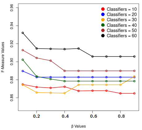
(a)

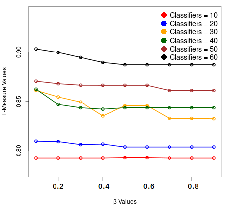
(b)

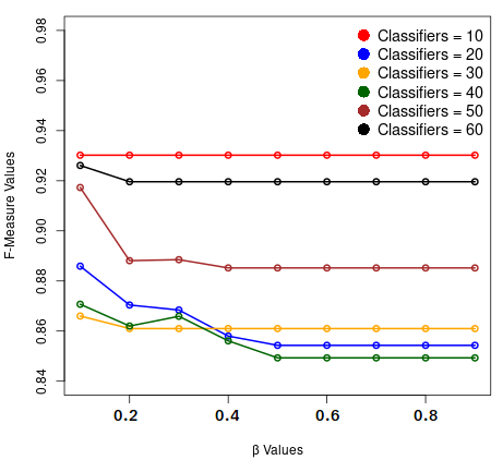
(c)

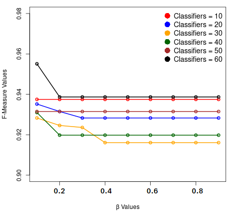
(d)

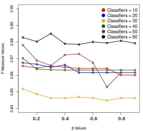
(e)

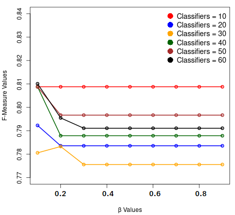
(f)

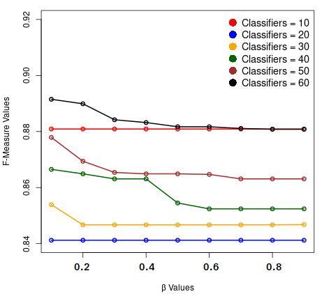
(g)

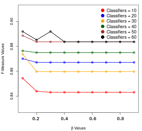
(h)

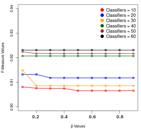
(i)

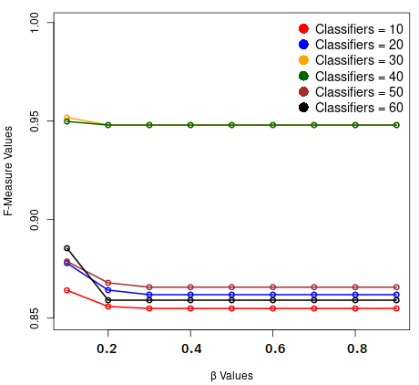
(j)

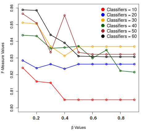
(k)

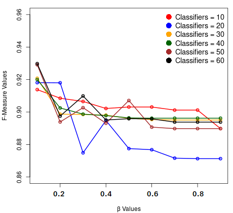
(l)

Figure 2: Variation in the F-measure values after experimenting PWMV at different values of $\beta$ and at using different number of diverse classifiers on the target projects.

As discussed in corollary 1, choosing the right value of $\beta$ in PWMV helps to improve the final performance of the HIEL model. Hence, to select the value of $\beta$, we have conducted an experiment on different sets of diverse classifiers based on F-measure on each target project. Nonetheless, the experimentation can also be conducted using other metrics. We then utilised different sets of diverse classifiers to provide generalizability in showing the performances. Since each target project has a different distribution of the data, we have conducted this experiment on each new version of the target project to select the value of $\beta$. Figure 2 represents the change in the performances of HIEL when utilising different values of $\beta$ at different sets of utilised diverse classifiers on the randomly selected target projects from the repositories PROMISE, NASA, and AEEEM, respectively.

It is observed from the Figure 2 that the performance of the HIEL model is high on the majority of the target projects at the $\beta$ value of 0.1, except on the projects Ant-1.7, Tomcat, and Velocity-1.6. On the projects Ant-1.7, Tomcat, and Velocity-1.6, the performance of the HIEL using PWMV is high at values of 0.9, 0.3, and 0.2, respectively. These performances are observed when utilising 30, 60, and 30 diverse classifiers on the above projects: Ant-1.7, Tomcat and Velocity-1.6, respectively. But on the target projects Tomcat and Velocity-1.6, the performance of HIEL at $\beta=0.1$ is just next to the performance of HIEL at $\beta=0.3$ and at $\beta=0.2$ respectively. In the project Ant-1.7, the performance of HIEL at $\beta=0.1$ stands in sixth place when we order the values of F-measure in decreasing order.

Precisely, when we consider each project, for example, in the case of Ant-1.7, out of six sets of diverse classifiers, the F-measure values are high at the $\beta=0.1$, except when HIEL is tested for the set of 30 diverse classifiers. In the cases of JEdit-4.3, Redaktor, Synapse-1.0, Tomcat, Xalan-2.4, Xerces-1.3, JM1, MW1, Eclipse, and Mlyn, the F-measure values are high at $\beta=0.1$ when using all sets of diverse classifiers. In the case of Velocity-1.6, the F-measure values of HIEL are incremented at $\beta=0.2$ when using the set of 30 diverse classifiers. On the other set of diverse classifiers (the case of Velocity-1.6), the F-measure values of HIEL were recorded high at $\beta=0.1$.

From figures 2 and 5, it is observed that, on the majority of the projects, the performances of HIEL using PWMV are recorded high at $\beta=0.1,0.2,$ and $0.3$, when utilising various sets of diverse classifiers. For the remaining values of $\beta$, the performance of HIEL gets decremented except in very few cases. Amongst the values of $\beta=0.1,0.2,$ and $0.3$, in the majority cases (on majority projects), the HIEL recorded its high F-measure values when using the value of $\beta=$ 0.1. Because, in the majority of cases, the F-measure values are high at $\beta=0.1$, in section 5.2, the comparative analysis is conducted using the proposed classification framework at $\beta=0.1$.

5.2 Comparative Analysis Using Traditional Measures

Table 5: Comparison of the proposed HIEL model with the other published models in terms of F-measure on PROMISE projects. The W/T/L indicates the proposed model won, tied, or lost to the other models

S.No	Project	CODEP	TCA+	HYDRA	TPTL	TDS	HIEL
1	Ant-1.3	0.2857	0.3689	0.468	0.456	0.2857	0.9321
2	Ant-1.4	0.2222	0.3816	0.914	0.377	0.2476	0.8704
3	Ant-1.5	0.2970	0.2956	0.691	0.237	0.2319	0.9149
4	Ant-1.6	0.5161	0.5419	0.807	0.595	0.4153	0.8313
5	Ant-1.7	0.4805	0.4896	0.295	0.455	0.3750	0.8489
6	Camel-1.0	0.0870	0.1194	0.529	0.093	0.0541	0.9755
7	Camel-1.2	0.1978	0.4189	0.19	0.502	0.4828	0.7837
8	Camel-1.4	0.2083	0.3750	0.503	0.339	0.2747	0.9127
9	Camel-1.6	0.1965	0.3514	0.991	0.356	0.2436	0.8884
10	Jedit-3.2	0.3862	0.6324	0.903	0.536	0.4828	0.7407
11	Jedit-4.0	0.4255	0.5194	0.6291	0.447	0.5054	0.8412
12	Jedit-4.1	0.4968	0.5333	0.551	0.522	0.4205	0.7967
13	Jedit-4.2	0.4295	0.3321	0.492	0.37	0.2172	0.8402
14	Jedit-4.3	0.0508	0.0461	0.324	0.05	0.0494	0.9033
15	Log4j-1.0	0.2273	0.5000	0.413	0.637	0.4356	0.8793
16	Log4j-1.1	0.2979	0.6957	0.538	0.699	0.4146	0.8421
17	Log4j-1.2	0.2569	0.6529	0.914	0.606	0.5387	0.1436
18	Lucene-2.0	0.2569	0.6593	0.648	0.569	0.6267	0.7259
19	Lucene-2.2	0.1707	0.6202	0.657	0.515	0.5447	0.5925
20	Lucene-2.4	0.2823	0.6593	0.691	0.458	0.3282	0.6138
21	Poi-1.5	0.2395	0.7390	0.742	0.713	0.4259	0.5895
22	Poi-2.0	0.3077	0.2439	0.283	0.218	0.2446	0.9029
23	Poi-2.5	0.2838	0.7723	0.78	0.728	0.7261	0.5443
24	Poi-3.0	0.3718	0.8303	0.807	0.787	0.7159	0.5537
25	Redaktor	0.2273	0.2344	0.295	0.353	0.2381	0.9172
26	Synapse-1.0	0.4865	0.2542	0.252	0.253	0.1064	0.9514
27	Synapse-1.1	0.3855	0.4583	0.494	0.475	0.4405	0.8611
28	Synapse-1.2	0.3276	0.5654	0.529	0.571	0.4664	0.8102
29	Tomcat	0.3907	0.2756	0.19	0.287	0.2626	0.8876
30	Velocity-1.4	0.2143	0.5726	0.793	0.734	0.3961	0.4257
31	Velocity-1.6	0.3333	0.5116	0.503	0.568	0.3587	0.8101
32	Xalan-2.4	0.3436	0.3924	0.315	0.403	0.3279	0.8915
33	Xalan-2.5	0.3366	0.5438	0.593	0.533	0.3944	0.6893
34	Xalan-2.6	0.3415	0.5210	0.656	0.512	0.4611	0.7021
35	Xalan-2.7	0.2697	0.6440	0.991	0.616	0.4036	0.7248
36	Xerces-1.2	0.2345	0.2266	0.24	0.192	0.2367	0.8889
37	Xerces-1.3	0.4027	0.3541	0.417	0.377	0.2297	0.8917
38	Xerces-1.4	0.3012	0.4934	0.903	0.69	0.7442	0.8163
	Average	0.3045	0.4691	0.5771	0.4692	0.3777	0.7825
	Improvement	155.89	66.11	35.02	66.07	106.32	-
	W/T/L	37/0/1	30/0/8	26/0/12	33/0/5	34/0/4	-
	p-value	1.55E-12	1.44E-09	1.40E-04	1.35E-09	3.28E-11	-
	Cliff’s Delta	0.9432	0.8075	0.5083	0.8089	0.8851	-

Table 6: Comparison of the proposed HIEL model with the other published models in terms of F-measure on the NASA-MDP projects. The W/T/L indicates the proposed model won, tied, or lost to the other models

S.No	Project	CODEP	TCA+	HYDRA	TPTL	TDS	HIEL
1	CM1	0.0769	0.2182	0.7899	0.8978	0.2338	0.8645
2	JM1	0.0334	0.3225	0.6897	0.7419	0.2138	0.8913
3	KC1	0.0180	0.3951	0.9014	0.6871	0.1901	0.882
4	KC3	0.0000	0.3051	0.7648	0.7889	0.2951	0.8162
5	MC1	0.0494	0.0350	0.8987	0.6982	0.0271	0.9848
6	MC2	0.1277	0.5301	0.7965	0.7849	0.4198	0.7586
7	MW1	0.0000	0.1888	0.8733	0.6911	0.1988	0.8611
8	PC1	0.1389	0.1629	0.8541	0.8922	0.1520	0.8788
9	PC2	0.0000	0.0416	0.8765	0.9154	0.0377	0.9946
10	PC3	0.0252	0.2422	0.9562	0.7912	0.2956	0.9347
11	PC4	0.0220	0.2662	0.8451	0.8629	0.1498	0.9291
12	PC5	0.1709	0.3876	0.8473	0.7696	0.1453	0.9847
	Average	0.0552	0.2579	0.8411	0.7934	0.1966	0.8984
	Improvement	1527.54	248.35	6.81	13.23	356.97	-
	W/T/L	12/0/0	12/0/0	8/0/4	9/0/3	12/0/0	-
	p-value	3.60E-05	7.40E-07	0.06836	0.01	7.40E-07	-
	Cliff’s Delta	1	1	0.4444	0.6111	1	-

Table 7: Comparison of the proposed HIEL model with the other published models in terms of F-measure on the AEEEM projects. The W/T/L indicates the proposed model won, tied, or lost to the other models

S.No	Project	CODEP	TCA+	HYDRA	TPTL	CODEP	HIEL
1	Eclipse	0.4709	0.3761	0.8612	0.8897	0.3939	0.8716
2	Equinox	0.2282	0.6887	0.7998	0.7114	0.5094	0.7631
3	Lucene	0.2529	0.3247	0.9247	0.8462	0.3094	0.9509
4	Mylyn	0.2186	0.3072	0.8618	0.7465	0.2530	0.9298
5	PDE	0.2699	0.3021	0.8984	0.7249	0.2941	0.9159
	Average	0.2881	0.3998	0.8692	0.7837	0.3520	0.8863
	Improvement	207.76	121.68	1.96	13.09	151.79	-
	W/T/L	5/0/0	5/0/0	4/0/1	4/0/1	5/0/0	-
	p-value	0.0079	0.0079	0.402	0.036	0.0079	-
	Cliff’s Delta	1	1	0.36	0.52	1	-

Table 8: Comparison of the proposed HIEL model with the other published models in terms of AUC on the PROMISE projects. The W/T/L indicates the proposed model won, tied, or lost to the other models

S.No	Project	CODEP	TCA+	HYDRA	TPTL	TDS	HIEL
1	Ant-1.3	0.5702	0.6702	0.8154	0.6545	0.5750	0.8329
2	Ant-1.4	0.4966	0.5618	0.6512	0.6121	0.4342	0.6685
3	Ant-1.5	0.6309	0.6986	0.6698	0.5589	0.6164	0.5715
4	Ant-1.6	0.6721	0.6978	0.7145	0.5846	0.6234	0.5925
5	Ant-1.7	0.6658	0.6966	0.7223	0.5899	0.5858	0.5663
6	Camel-1.0	0.5294	0.6344	0.6541	0.5001	0.3992	0.681
7	Camel-1.2	0.5242	0.5431	0.6248	0.6148	0.5639	0.6255
8	Camel-1.4	0.5381	0.6418	0.8847	0.5877	0.5363	0.9197
9	Camel-1.6	0.5301	0.5862	0.6088	0.5981	0.6033	0.6096
10	Jedit-3.2	0.5814	0.7164	0.6973	0.5549	0.5789	0.5808
11	Jedit-4.0	0.6221	0.6956	0.7111	0.6154	0.6661	0.642
12	Jedit-4.1	0.6631	0.7003	0.5122	0.5527	0.5816	0.5601
13	Jedit-4.2	0.7252	0.6898	0.5009	0.5879	0.5387	0.5376
14	Jedit-4.3	0.5283	0.5209	0.5121	0.5262	0.5333	0.513
15	Log4j-1.0	0.5488	0.6648	0.6712	0.6346	0.5504	0.8915
16	Log4j-1.1	0.5738	0.7727	0.6939	0.6187	0.5439	0.8564
17	Log4j-1.2	0.5428	0.5326	0.7856	0.6909	0.4127	0.5006
18	Lucene-2.0	0.5577	0.6806	0.6545	0.6155	0.6298	0.7326
19	Lucene-2.2	0.5195	0.6127	0.6333	0.6406	0.5284	0.5853
20	Lucene-2.4	0.5497	0.6459	0.5877	0.5641	0.5334	0.5899
21	Poi-1.5	0.5397	0.6521	0.6849	0.6711	0.5020	0.5972
22	Poi-2.0	0.6098	0.5823	0.5588	0.6667	0.6167	0.5784
23	Poi-2.5	0.5429	0.6669	0.5501	0.6319	0.6395	0.5952
24	Poi-3.0	0.5926	0.7757	0.7889	0.6244	0.6495	0.6125
25	Redaktor	0.5140	0.4892	0.5589	0.5445	0.6225	0.7091
26	Synapse-1.0	0.7387	0.6602	0.6696	0.5654	0.4654	0.766
27	Synapse-1.1	0.6117	0.5951	0.6562	0.5228	0.5634	0.7677
28	Synapse-1.2	0.5781	0.6425	0.5941	0.6207	0.5319	0.6924
29	Tomcat	0.7113	0.7135	0.5846	0.6349	0.6907	0.5259
30	Velocity-1.4	0.5306	0.4796	0.6609	0.7129	0.4352	0.5708
31	Velocity-1.6	0.5756	0.6165	0.5843	0.6848	0.3957	0.6873
32	Xalan-2.4	0.6137	0.7017	0.509	0.5678	0.5937	0.5708
33	Xalan-2.5	0.5654	0.5644	0.6967	0.6509	0.5157	0.73
34	Xalan-2.6	0.5780	0.5477	0.5999	0.6333	0.5746	0.6717
35	Xalan-2.7	0.5780	0.6923	0.7333	0.5147	0.8334	0.5062
36	Xerces-1.2	0.5425	0.5143	0.5213	0.5411	0.4252	0.5859
37	Xerces-1.3	0.6523	0.6340	0.5708	0.5379	0.3544	0.5449
38	Xerces-1.4	0.5793	0.6021	0.6159	0.5978	0.4093	0.5786
	Average	0.5848	0.6340	0.6386	0.6007	0.5488	0.6407
	Improvement	9.56	1.06	0.33	6.67	16.76	-
	W/T/L	24/0/14	18/0/20	24/0/14	26/0/12	24/0/14	-
	p-value	0.01322	0.5503	0.5195	0.2553	0.0007	-
	Cliff’s Delta	0.3311	-0.0803	-0.0865	0.1524	0.4516	-

Table 9: Comparison of the proposed HIEL model with the other published models in terms of AUC on the NASA projects.The W/T/L indicates the proposed model won, tied, or lost to the other models

S.No	Project	CODEP	TCA+	HYDRA	TPTL	TDS	HIEL
1	CM1	0.5106	0.5017	0.61	0.6218	0.5678	0.5516
2	JM1	0.5081	0.5314	0.5212	0.5451	0.4612	0.5151
3	KC1	0.5032	0.7057	0.5146	0.512	0.575	0.5234
4	KC3	0.5000	0.5000	0.5226	0.5224	0.5750	0.5335
5	MC1	0.5141	0.7621	0.5349	0.5759	0.6016	0.5034
6	MC2	0.5341	0.5301	0.6265	0.6117	0.5806	0.6265
7	MW1	0.5000	0.5105	0.5601	0.5159	0.5359	0.5502
8	PC1	0.5367	0.5509	0.5419	0.5264	0.5440	0.552
9	PC2	0.5000	0.7648	0.5058	0.6157	0.5430	0.5105
10	PC3	0.4985	0.5553	0.6578	0.6099	0.5985	0.7292
11	PC4	0.5048	0.5962	0.6673	0.6144	0.4588	0.6355
12	PC5	0.5494	0.9119	0.5837	0.5431	0.5413	0.61
	Average	0.5133	0.6184	0.5705	0.5679	0.5486	0.5701
	Improvement	11.07	-7.81	-0.07	0.39	3.92	-
	W/T/L	11/0/1	7/0/5	6/1/5	8/0/4	7/0/5	-
	p-value	0.0035	0.729	0.8852	0.9323	0.8398	-
	Cliff’s Delta	0.7083	-0.0903	-0.0416	-0.0278	0.0556	-

Table 10: Comparison of the proposed HIEL model with the other published models in terms of AUC on the AEEEM projects. The W/T/L indicates the proposed model won, tied, or lost to the other models

S.No	Project	CODEP	TCA+	HYDRA	TPTL	TDS	HIEL
1	Eclipse	0.6636	0.5713	0.5957	0.6259	0.6378	0.6173
2	Equinox	0.5582	0.7262	0.6641	0.6241	0.6391	0.6945
3	Lucene	0.5764	0.7138	0.6412	0.6887	0.6485	0.7273
4	Mylyn	0.5595	0.6108	0.6514	0.5679	0.5702	0.5723
5	PDE	0.5769	0.6177	0.5521	0.5659	0.6046	0.5364
	Average	0.5869	0.6480	0.6209	0.6145	0.6200	0.6296
	Improvement	7.27	-2.84	1.39	1.04	1.53	-
	W/T/L	3/0/2	2/0/3	3/0/2	2/0/3	3/0/2	-
	p-value	0.5476	0.8413	1	1	1	-
	Cliff’s Delta	0.28	-0.12	0.04	0.04	0.04	-

After selecting the value of $\beta$, we have compared the proposed HIEL (which is constructed using a set of 60 diverse classifiers) with the other baseline models on the target projects selected from the publicly available repositories such as PROMISE, NASA, and AEEEM. The comparative analysis is conducted with works such as TDS, TCA+, CODEP, HYDRA, and TPTL. The comparative analysis is conducted using measures such as F-measure and AUC. In [19], Herbold et al. conducted a large scale empirical survey on the cross project defect prediction studies and replicated 24 approaches that were published between 2008 and 2015. Amongst the replicated models, we have utilised the F-measure and AUC values directly from the replicated works of TDS, TCA+, and CODEP on PROMISE, NASA, and AEEEM datasets. Because, irrespective of utilising the training set, each of the above models computes the final performance on the same target project. And for the works HYDRA and TPTL, we used publicly available source code provided by the respective authors.

Tables 5, 6, and 7 represent the F-measure values of various models on the PROMISE, NASA, and AEEEM projects, respectively. From table 5, it is observed that, on many target PROMISE projects, the proposed HIEL model shows a substantial improvement over the other base-line models, significantly. On an average across 38 PROMISE projects, the proposed HIEL model achieved an improvement of 155.89%, 66.11%, 35.02%, 66.07%, and 106.32% on the base-line models such as CODEP, TCA+, HYDRA, TPTL, and TDS, respectively. Similar results have been observed in NASA projects also. From the table 6, it is observed that, on an average across 12 NASA projects, the proposed HIEL model achieved an improvement of 1527.54%, 248.35%, 6.81%, 13.23%, and 356.97% on the base-line models such as CODEP, TCA+, HYDRA, TPTL, and TDS, respectively. Similarly, from table 7, it is observed that, on the 5 AEEEM projects, on an average, the proposed HIEL model achieved an improvement of 207.76%, 121.68%, 1.96%, 13.09%, and 151.79% on the base-line models such as CODEP, TCA+, HYDRA, TPTL, and TDS, respectively.

Tables 8, 9, and 10 represent the AUC values of various models on the PROMISE, NASA, and AEEEM projects, respectively. The performances (in terms of AUC) of all the models on NASA and AEEEM projects indicate the competitive outcomes. From table 8, it is observed that, on many target PROMISE projects, the proposed HIEL model shows a little improvement over the other base-line models. On an average across 38 PROMISE projects, the proposed HIEL model achieved an improvement of 9.56%, 1.06%, 0.33%, 6.67%, and 16.76% on the base-line models such as CODEP, TCA+, HYDRA, TPTL, and TDS respectively. From table 9, it is observed that, on an average across 12 NASA projects, the proposed HIEL model achieved an improvement of 11.06%, 0.39%, and 3.92% over the base-line models such as CODEP, TPTL, and TDS respectively. But the models TCA+ and HYDRA are showing their better performances over the proposed HIEL model. From table 10, it is observed that, on the 5 AEEEM projects, on an average, the proposed HIEL model achieved an improvement of 7.27%, 1.39%, 1.04%, and 1.53% on the base-line models such as CODEP, HYDRA, TPTL, and TDS, respectively. In this case, the model TCA+ is showing its better performance over the proposed HIEL model.

The tables 5, 6, and 7 also present the results of the significant tests (conducted using F-measure) such as the one-sample Wilcoxson signed rank test and Cliff’s delta effect size test. It is observed from the table 5 that, the proposed model shows its significant improvement in terms of F-measure over all the other models. The values of Cliff’s delta also indicate the large effect among the models. On NASA projects (from the table 6), except on HYDRA, the proposed model achieved significantly better results. Despite the fact that the Wilcoxson signed rank test finds no significant difference between HYDRA and HIEL ($p=0.0684>0.05$), the Cliff’s delta effect size test finds a medium effect for the HIEL ($delta=0.444$) when compared to the HYDRA model. The table 7 also indicate the similar results. On AEEEM projects, except on HYDRA, the proposed model achieved significantly better results in terms of F-measure. Even though there is no significant difference between HYDRA and HIEL performances, ($p=0.402>0.05$) is observed according to the Wilcoxson signed rank test, the Cliff’s delta effect size test shows that the HIEL has a medium effect ($\delta=0.36$) when compared with the HYDRA model.

Similarly, the tables 8, 9, and 10 also present the results of the significant tests (conducted using AUC) such as the one-sample Wilcoxson signed rank test and Cliff’s delta effect size test. It is observed from the table 8, that the proposed model shows a significant improvement in the performances in terms of AUC on the models such as CODEP and TDS. The values of Cliff’s delta also indicate the large effect among these models. On the other models, the HIEL does not show its significance difference in terms of both the tests.

From the table 9, on NASA projects, it is observed that, when compared with the CODEP model, the proposed model achieved significantly better average performance in terms of the Wilcoxson signed rank test and Cliff’s delta effect size test. On the other models such as TCA+, HYDRA, TPTL, and TDS, the HIEL does not show a significant difference in the performances in terms of both the tests. From table 10, we observe on AEEEM projects that, even though the proposed model achieved better average AUCs, it does not achieve significantly better results in terms of either of the tests.

In summary, on some models, even though the proposed model is incapable of producing significant results in terms of AUC, it is showing a significantly better improvement in the average performance (in terms of F-measure) than the other models.

5.3 The Saved Budget, Remaining Service Time and Failure Analysis

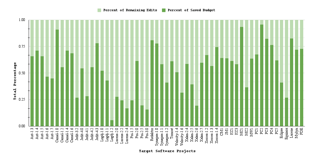
Figure 3: The percent of saved budget (PSB) and the percent of remaining edits (PRE), obtained from the HIEL model on all the target projects

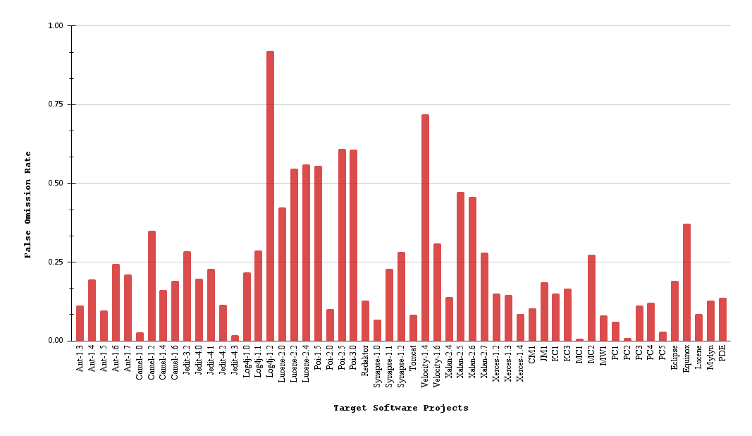
Figure 4: The false omission rates (FOR) obtained from the HIEL model on all the target projects.

Table 11: The supplementary details of the proposed measures

PROMISE Projects
S.No	Project	Total LoC	Defects	Saved Budget	Remaining Service Time	Project Hours	Original Editing Rate	Editing Rate	Decreased Editing Rate
1	Ant-1.3	37699	20	24755	12944	129.44	1884.95	647.20	1237.75
2	Ant-1.4	54195	40	38528	15667	156.67	1354.88	391.68	963.20
3	Ant-1.5	87047	32	57345	29702	297.02	2720.22	928.19	1792.03
4	Ant-1.6	113246	92	52707	60539	605.39	1230.93	658.03	572.90
5	Ant-1.7	208653	166	93929	114724	1147.24	1256.95	691.11	565.84
6	Camel-1.0	33721	13	30679	3042	30.42	2593.92	234.00	2359.92
7	Camel-1.2	66302	216	36764	29538	295.38	306.95	136.75	170.20
8	Camel-1.4	98080	145	69685	28395	283.95	676.41	195.83	480.59
9	Camel-1.6	113055	188	77510	35545	355.45	601.36	189.07	412.29
10	Jedit-3.2	128883	90	34674	94209	942.09	1432.03	1046.77	385.27
11	Jedit-4.0	144803	75	78584	66219	662.19	1930.71	882.92	1047.79
12	Jedit-4.1	153087	79	43047	110040	1100.40	1937.81	1392.91	544.90
13	Jedit-4.2	170683	48	94791	75892	758.92	3555.90	1581.08	1974.81
14	Jedit-4.3	202363	11	158076	44287	442.87	18396.64	4026.09	14370.55
15	Log4j-1.0	21549	34	11220	10329	103.29	633.79	303.79	330.00
16	Log4j-1.1	19938	37	8537	11401	114.01	538.86	308.14	230.73
17	Log4j-1.2	38191	189	2103	36088	360.88	202.07	190.94	11.13
18	Lucene-2.0	50596	91	13920	36676	366.76	556.00	403.03	152.97
19	Lucene-2.2	63571	144	15384	48187	481.87	441.47	334.63	106.83
20	Lucene-2.4	102859	203	17128	85731	857.31	506.69	422.32	84.37
21	Poi-1.5	55428	141	13422	42006	420.06	393.11	297.91	95.19
22	Poi-2.0	93171	37	57128	36043	360.43	2518.14	974.14	1544.00
23	Poi-2.5	119731	248	21104	98627	986.27	482.79	397.69	85.10
24	Poi-3.0	129327	281	20275	109052	1090.52	460.24	388.09	72.15
25	Redaktor	59280	27	47876	11404	114.04	2195.56	422.37	1773.19
26	Synapse-1.0	28806	16	22391	6415	64.15	1800.38	400.94	1399.44
27	Synapse-1.1	42302	60	24610	17692	176.92	705.03	294.87	410.17
28	Synapse-1.2	53500	86	21963	31537	315.37	622.09	366.71	255.38
29	Tomcat	300674	77	183474	117200	1172.00	3904.86	1522.08	2382.78
30	Velocity-1.4	51713	147	26258	25455	254.55	351.79	173.16	178.63
31	Velocity-1.6	57012	78	17946	39066	390.66	730.92	500.85	230.08
32	Xalan-2.4	225088	110	131695	93393	933.93	2046.25	849.03	1197.23
33	Xalan-2.5	304860	387	119902	184958	1849.58	787.75	477.93	309.82
34	Xalan-2.6	411737	411	78959	332778	3327.78	1001.79	809.68	192.11
35	Xalan-2.7	428555	898	256233	172322	1723.22	477.23	191.90	285.34
36	Xerces-1.2	159254	71	106330	52924	529.24	2243.01	745.41	1497.61
37	Xerces-1.3	167095	69	94588	72507	725.07	2421.67	1050.83	1370.84
38	Xerces-1.4	141180	437	105066	36114	361.14	323.07	82.64	240.43
	Total	4737234	5494	2308586	2428648	24286.48	66224.21	24910.68	41313.53
NASA Projects
1	CM1	15486	42	9925	5561	55.61	368.71	132.40	236.31
2	JM1	376794	1759	240094	136700	1367.00	214.21	77.71	136.49
3	KC1	42706	325	26221	16485	164.85	131.40	50.72	80.68
4	KC3	6399	36	3734	2665	26.65	177.75	74.03	103.72
5	MC1	66583	68	62137	4446	44.46	979.16	65.38	913.78
6	MC2	5503	44	2006	3497	34.97	125.07	79.48	45.59
7	MW1	6905	27	4390	2515	25.15	255.74	93.15	162.59
8	PC1	23020	61	15499	7521	75.21	377.38	123.30	254.08
9	PC2	17834	16	17069	765	7.65	1114.63	47.81	1066.81
10	PC3	33016	140	27151	5865	58.65	235.83	41.89	193.94
11	PC4	30055	178	22981	7074	70.74	168.85	39.74	129.11
12	PC5	161695	516	99849	61846	618.46	313.36	119.86	193.51
	Total	785996	3212	531056	254940	2549.40	4462.09	945.48	3516.61
AEEEM Projects
1	Eclipse	224055	206	91682	132373	1323.73	1087.65	642.59	445.06
2	Equinox	39534	129	10541	28993	289.93	306.47	224.75	81.71
3	Lucene	73184	64	60449	12735	127.35	1143.50	198.98	944.52
4	Mylyn	156102	245	112333	43769	437.69	637.15	178.65	458.50
5	PDE	146952	209	106900	40052	400.52	703.12	191.64	511.48
	Total	639827	853	381905	257922	2579.22	3877.88	1436.61	2441.27

This section describes the proposed HIEL model’s performance in terms of the proposed measures.

The figure 3 depicts the percent of saved budget and the percent of remaining edit ratios, which are obtained from the HIEL model on all the datasets. It is observed from the figure 3 that, out of 55 target projects, 36 target projects account for more than 50% of the budget savings from the HIEL model. Within the 36 projects, 9 projects such as Camel-1.0, JEdit-4.3, Redaktor, Synapse-1.0, MC1, PC2, PC3, PC4, and Lucene account for more than 75% of the budget savings from the original allocated budget. Surprisingly, the projects Camel-1.0, MC1, and PC2 greatly benefit from the use of the HIEL model, as these projects account for more than 90% of the budget savings from the original allocated budget.

The figure 3 also represents the amount of service time required to remove the defect content. The vertical bars on top of the dark green bars indicate the percent of remaining edits that are present in each target project. From the figure 3, it is observed that the testers need to conduct more than 50% code-walk on 19 projects to observe the total defects in the respective projects. Of which, only 7 projects, such as Log4j-1.2, Lucene-2.2, Lucene-2.4, Poi-1.5, Poi-2.5, Poi-3.0, and Xalan-2.6 require more than 75% of the code walk to observe the total defects. Among the 7 projects, Log4j-1.2 requires more than 90% of the code-walk to observe the total defects.

Table 11 presents the supplementary details of the proposed measures. These details provide more insights on the predictions. From the table 11, it is observed that, on an average, the HIEL on the PROMISE projects contributes to 49.70% of the total savings (nearly 2.3 million cost units out of 4.7 million allocated cost units). The remaining 50.30% lines of code (nearly 2.4 million LoC) need to be investigated by the testers to observe the defects. This is equivalent to the testers spending 24,286 hours of time (assume, from equation 19, a group of testers service 100 LoC ($\delta=100$) in an hour) on the respective modules. In the process of conducting the code-walk, on an average, for every 24,911 LoC, the testers will find one defect. If the group of testers would involved in testing the same developed code, then the original editing rate to observe one defect is approximately 66,225 LoC/defect. Hence, by using the HIEL model, on an average, the testers can avoid nearly 41,314 edits.

On NASA and AEEEM projects (from the table 11), the HIEL model attributes to an improved budget savings of 68.70% cost units (531,056 cost units out of 785,996 allocated cost units). On the remaining 31.30% of the LoC (254,940 time units), the testers need to investigate such code to observe the defects. This is equivalent to the testers spending 2549 hours of time on the respective modules. In the process of conducting the code-walk, on an average, for every 945 LoC, the testers will find one defect. If the group of testers were involved in testing the same developed code, then the original editing rate to observe one defect is approximately 4462 LoC/defect. Hence, by using the HIEL model, on an average, the testers can avoid nearly 3517 edits.

Similarly, on the AEEEM projects, the HIEL tries to save 58.98% of the budget (which is equivalent to 381,905 cost units) and leaves the testers about 41.02% of the LoC (which is equivalent to 257,922 time units) for the investigation of the defects. In this case, for the complete code-walk, the testers have to engage with the code for nearly 2579 hours of time to detect the complete defects. While conducting the code-walk, on an average, the testers may observe one defect for every 1437 LoC. If the group of testers were involved in testing the same developed code, then the original editing rate to observe one defect is approximately 3878 LoC/defect. Hence, by using the HIEL model, on an average, the testers can avoid nearly 2441 edits. However, to achieve the desired goal of the defect prediction task, the prediction model should have to reduce the remaining service time (consequently, it improves the savings in the total allocated budget) to the maximum possible extent.

On the other hand, the figure 4 represents the failure rate (in terms of FOR) in each target project. From the figure 4, it is observed that, among all the target projects, the projects such as Log4j-1.2, Lucene-2.2, Lucene-2.4, Poi-1.5, Poi-2.5, Poi-3.0, and Velocity-1.4 may experience more than 50% of the failure incidents, due to dormant defects. Among which, the project Log4j-1.2 has more than 90% failure incidents. Note that, because each project is different in size (in terms of modules and the number of defects), the above mentioned percentages are proportional to the failure condition of the individual project. In total, the HIEL results in 5494, 3212, and 853 hidden defects (dormant defects) in the PROMISE, NASA, and AEEEM projects, respectively. On an average, this is equivalent to 28.44%, 10.87%, and 18.30% of the failure chances in the PROMISE, NASA, and AEEEM projects, respectively. However, to achieve a safe system, the prediction model needs to nullify the number of failure conditions (that is, FOR) from the predictions.

5.4 Comparative Analysis Using Proposed Measures

Table 12: Average performances of the models such as HIEL, HYDRA, TPTL in terms of the proposed measures.

		PPC			PSB			PNPC			PRE			FOR
S.No	Repository	HIEL	HYDRA	TPTL	HIEL	HYDRA	TPTL	HIEL	HYDRA	TPTL	HIEL	HYDRA	TPTL	HIEL	HYDRA	TPTL
1	PROMISE	0.6455	0.4547	0.3517	0.4970	0.3260	0.3129	0.3545	0.5453	0.6483	0.5030	0.6740	0.6871	28.44	28.29	30.66
2	NASA	0.8023	0.7089	0.6720	0.6870	0.6099	0.5329	0.1977	0.2911	0.3280	0.3130	0.3901	0.4671	10.87	10.73	12.90
3	AEEEM	0.7826	0.7495	0.6650	0.5898	0.5355	0.5198	0.2174	0.2505	0.3350	0.4102	0.4645	0.4802	18.30	17.96	20.17
	Average	0.7435	0.6377	0.5629	0.5913	0.4905	0.4552	0.2565	0.3623	0.4371	0.4087	0.5095	0.5448	19.20	18.99	21.24
	Improvement	-	16.59% $\Uparrow$	32.08%$\Uparrow$	-	20.55%$\Uparrow$	29.90%$\Uparrow$	-	41.25%$\Downarrow$	70.41%$\Downarrow$	-	24.66%$\Downarrow$	33.30%$\Downarrow$	-	1.11%$\Downarrow$	10.63%$\Downarrow$
The green-coloured arrows (both up and down arrows) indicates that the proposed model achieved better performances than the other models. The red-
coloured arrow indicates that the proposed model does not achieve better performance over the other model.

In section 5.2, we have provided the comparative analysis using the traditional measures such as F-measure and AUC. In this section, we present a comparative analysis using the proposed measures. As an example, the comparative analysis is provided between the three approaches, such as TPTL, HYDRA, and the proposed HIEL model. We have chosen two models such as HYDRA and TPTL, because from the empirical evaluations (in section 5.2), it is observed that these two models are the strongest competitors to our proposed approach. Nonetheless, numerous approaches may utilise the proposed measures to evaluate the predictions.

Table 12 presents the average performances of the proposed HIEL model, along with HYDRA and TPTL, respectively, on the three repositories such as PROMISE, NASA, and AEEEM, using the proposed measures. When compared with the traditional measures, in the majority of cases, the proposed model shows a clear improvement in terms of the proposed measures on the base-lines such as HYDRA and TPTL. From table 12, it is observed that, on an average across all the repositories, the proposed HIEL model achieved an improvement of 16.59% and 32.08%, respectively, over the base-line models such as HYDRA and TPTL, respectively, in terms of the percent of perfect cleans. This is an indication of accurate predictions in terms of actual clean modules. Hence, consequently, the proposed model is showing an improvement of 20.55% and 29.90%, respectively, over the base-line models such as HYDRA and TPTL, in terms of the percent of saved budget. This indicates that, with the use of the proposed model, on an average, the target projects may benefit in terms of savings in the total allocated budget.

Similarly, from table 12, it is observed that, on an average across all the repositories, the proposed HIEL model achieved an improvement of 41.25% and 70.41%, respectively, over the base-line models such as HYDRA and TPTL, in terms of the percent of non-perfect cleans. This indicates that, when compared with the other models, on average, the proposed model is more accurate in predicting the defective instances. Hence, consequently, the proposed model is showing an improvement of 24.66% and 33.30%, respectively, over the base-line models such as HYDRA and TPTL, in terms of the percent of remaining edits. This indicates that, when compared with the other models, on average, the testers may benefit in terms of savings in the remaining edits on the target projects.

In terms of average failure cases (that is, FOR) across all the target projects, the HYDRA model outperformed the other models. However, the HYDRA model when compared with the proposed model, achieved a negligible improvement of 1.11% on the average of all the target projects. This shows that, on an average, the HYDRA model is faintly better at reducing false negative instances on the majority of the target projects. But when compared with the TPTL model, the proposed model shows an improvement of 10.63% on the average of all the target projects. In summary, on an average across all utilised projects, when compared in terms of savings in the allocated budget and the remaining edits, the proposed model is clearly showing its improvement over the base-lines such as HYDRA and TPTL.

5.5 Discussion

5.5.1 On the Performance of HIEL using PWMV

In section 5.2, we have seen the comparative analysis of the HIEL over the other models. In this section, we discuss the change in the performance with the use of different sets of diverse inducers in the proposed HIEL model.

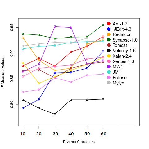
(a)

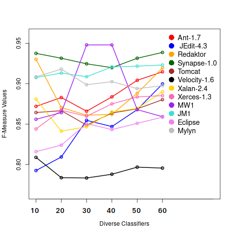
(b)

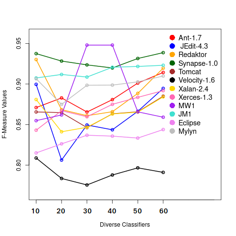
(c)

Figure 5: Variation in the F-measure values of HIEL using PWMV on 12 randomly selected projects (from three repositories) at different values of $\beta$. For each project, the performances are represented in a line of points for each set of utilised diverse classifiers

From the figure 5 it is observed that the performances on the target projects are proportional to the utilisation of a diverse set of classifiers. This satisfies the definition of ensemble learning, as the number of diverse classifiers increases infinitely, then the final decision on the test observation approaches to 1. From the experiments, it is observed that, except for the few projects, the final performances are increased as a result of an increase in the diverse set of classifiers. For example, on the project Redaktor, at $\beta=0.1$, the F-measure value obtained is 0.9302 when utilising the set of 10 diverse classifiers, which is higher than the value of F-measure when utilising the set of 60 diverse classifiers. From the corollary 1, we derive an analysis that, if the expert (taken from any set of inducers) is continuously making mistakes, then it is penalised with the decremented weights. Hence, in very few cases like the above, few decision makers may participate in obtaining the final decision.

Similarly, at $\beta=0.2$, the performances on all the target projects are proportional to the utilised diverse set of classifiers except for the projects Redaktor, Veocity-1.6, and Mylyn. When using the set of 60 different classifiers, projects such as JEdit-4.3, Redaktor, Veocity-1.6, and Mylyn obtained decremented F-measure values at $\beta=0.3$. In other cases, the projects show better performances with the use of more diverse classifiers. This indicates the advantage of using more diverse classifiers to obtain generalizable solutions on the target datasets.

5.5.2 On the Comparison Between the Performance Measures

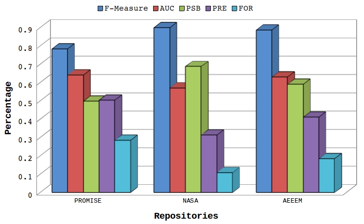
Figure 6: The traditional and proposed measures on all the target projects

In section 5.3, we have provided the experimental evaluations in terms of savings in the allocated total budget (using PSB/Saved budget) and the editing rates to achieve a failure-free software system. In this section, we discuss the utilised performance measures.

Figure 6 represents the average performance of HIEL (in terms of all the utilised measures), observed on the projects of PROMISE, NASA, and AEEEM repositories. From the table 6, it is observed that, even though the HIEL model exhibits the better F-measure and AUC values on all the repositories, the measures such as PSB and PRE indicate nearly half the benefits on the PROMISE projects. That is, on PROMISE projects, the testers still need to put effort into more than half the original code to remove the defects. In terms of PSB and PRE, the HIEL produces the best results on NASA and AEEEM projects. In addition to that, on an average, the failure rates in NASA are low when compared with the failure rates in the PROMISE and AEEEM repositories.

However, the above results show that, while traditional measures produce better results, these measures also provide an additional analysis of the obtained performances. Hence, in a critical application like SDP (in this case, CPDP), to understand the true benefits of the prediction model, we suggest using the proposed measures such as PSB, PRE, and FOR in addition to the traditional measures.

6 Threats to Validity

Since this model builds up on the machine learning model, it is inevitable to observe variation in the final performance at various implementation conditions. Consequently, this prediction result may have an impact on the saved budget, remaining service time, and the percent of failures in the target project. For this, the threats to the validity of the proposed model, such as construct validity in 6.1, internal validity in 6.2, and external validity in 6.3, are discussed.

6.1 Construct Validity

The projects in PROMISE, NASA, and AEEEM have limited metrics. Inclusion of a greater number of metrics may affect the final performance of HIEL. From the definition of ensemble learning, the model correctly predicts a class label for the test example if the number of classifiers approaches infinity. But this work utilises up to 60 diverse classifiers (for different experiments) to observe the final decision. However, variation in the performance of the proposed model may be observed by using a number of diverse classifiers other than 60. But, if the number of diverse classifiers increases in the ensemble, then the computational complexity of the ensemble algorithm (for instance, HIEL) also increases; hence, the time required to observe the decision increases. Therefore, a trade-off between the diverse classifiers and the computational complexity needs to be achieved to obtain better performances.

6.2 Internal Validity

Before training the proposed HIEL model, an optional feature reduction stage can be incorporated to select the relevant features from the original defect data. The studies such as [41, 42] suggests to incorporate this optional step to analyse the variation in the performance of the proposed model. Hence, there is a chance of getting improved results for the proposed model that uses any one of the feature reduction algorithms as the preprocessing stage. In contrast to incorporating the feature reduction schemes, selecting specific features such as combination of size, complexity, and object-oriented metrics [30] can also be evaluated prior to training the proposed model to observe the variation in the final prediction performance. Since each classification model differs from the implementation of the other, it is important to investigate the use of implementing feature reduction algorithms as well as the use of specific metrics such as object-oriented metrics and some size metrics as features in the proposed model.

To generate the diverse classifiers, the proposed model uses six inducers such as LR, SVM, DT, NB, K-NN, and NN. Nonetheless, the model can be built with the use of other inducers. As decision-makers increase (preferably weak inducers) in the ensemble model, then, the probability of getting the correct decision approaches 1. Hence, there is a chance of getting better performance when the proposed model is tested along with the other inducers.

To train the HIEL model, we have incorporated two diversity generation mechanisms, such as bootstrapping and hybrid-inducers, to generate the bag of classifiers. Nonetheless, the prediction performance of HIEL may be enhanced by including other diversity generation mechanisms such as optimising the learning parameters, feature subspace sampling, and changing the output representation methods. But the inclusion of these schemes will increase the computational overhead.

6.3 External Validity

To know the effectiveness of the proposed model, we compared it with the limited exiting works for CPDP. The robustness of the proposed model will be determined when it is compared with the large number of base-line classifiers and various classic ensemble models.

To find the transferability of the proposed approach, in the case of PWMV in HIEL, it has to be tested with the other categories of the training data such as defect severity data and heterogeneous defect data.

7 Conclusion and Future Works

This paper presents a novel hybrid-inducer ensemble learning (HIEL) method for cross-project defect prediction, that uses bootstrap aggregation of the source project’s defects data. Using the proposed method, a bag of 60 classifiers is generated by employing six inducers, each with ten training samples. Later, the probabilistic weighted majority voting technique (PWMV) is used as a combiner method on the generated classifiers to get the final decision for the test instance. Using PWMV, during the classification stage, a tight upper bound on the number of mistakes made by the best expert (classifier) taken from the proposed HIEL model is derived. We also conducted an empirical evaluation to analyse the variation in the performance of PWMV on the publicly available defect repositories such as PROMISE, NASA, and AEEEM. To validate the HIEL model, a comparative analysis was conducted with the recently published models such as TDS, TCA+, HYDRA, TPTL, and CODEP. Using the empirical analysis on the datasets, the following vital findings are observed:

• On the many PROMISE, NASA, and AEEEM projects, the HIEL model with PWMV achieved an improved average in-terms of both F-measure and AUC when compared with the other published CPDP models. Among the published models, in terms of AUC, the TCA+ and HYDRA stand as strong competitors to the HIEL model.

• The empirical analysis indicates the advantage of utilising the diversity-based ensemble models for this problem context. From the experimentation on utilising the different sets of diverse classifiers in the PWMV model, it is observed that the obtained performances are proportional to the utilised diverse classifiers on the target projects. Hence, building complex diverse classifiers has good potential for classifying the defect-proneness of the software module.

This work also aims to fill the gap in analysing the results of the CPDP model on developing software. While the traditional performance measures provide information about the working of the machine learning model, in this work, by making use of the LoC of the test module along with the information from the confusion matrix, the new perspectives from the predictions have been investigated through three performance measures such as PPC, PNPC, and FOR. Since LoC acts as an additional attribute along with the information from the confusion matrix, these performance metrics are treated as application-dependent measures. That is, these are applicable only to the binary classification of defect prediction models.

Among the proposed measures, the PPC helps to provide information about the percent of the budget saved, where as the PNPC measure helps to calculate the amount of work still remaining in the newly developed software project, by utilising the CPDP models. The FOR measure is used to estimate the number of failures that may occur in the developed software. As maximising the budget savings and minimising the remaining service time and failures are the primary goals in introducing SDP research, we recommend future research on SDP (any category, such as WPDP or CPDP) to focus on providing such model-specific outcome analysis.

7.1 Future Directions

The possible future directions in this research include: finding the defect associations from the predicted result of our proposed CPDP model, which is the immediate future objective. Finding the severity of the defective module once it is identified as defective by the SDP model, estimating the reliability of the software system after the deployment of the SDP model, etc. are still open challenges in this research field, on which we will focus our future research directions.

References

- [1] M. R. Lyu, et al., Handbook of software reliability engineering, Vol. 222, IEEE computer society press CA, 1996.
- [2] Q. Song, Z. Jia, M. Shepperd, S. Ying, J. Liu, A General Software Defect-Proneness Prediction Framework, IEEE Transactions on Software Engineering 37 (3) (2011) 356–370.
- [3] W. E. Wong, R. Gao, Y. Li, R. Abreu, F. Wotawa, A survey on software fault localization (2016).
- [4] S. Lessmann, B. Baesens, C. Mues, S. Pietsch, Benchmarking classification models for software defect prediction: A proposed framework and novel findings, IEEE Transactions on Software Engineering 34 (4) (2008) 485–496.
- [5] M. Monperrus, Automatic Software Repair: A Bibliography, ACM Computing Surveys 51 (1) (2018) 17:1—-17:24.
- [6] F. Wu, X.-Y. Jing, Y. Sun, J. Sun, L. Huang, F. Cui, Y. Sun, Cross-project and within-project semi-supervised software defect prediction: A unified approach, IEEE Transactions on Reliability 67 (2) (2018) 581–597.
- [7] N. E. Fenton, M. Neil, A Critique of Software Defect Prediction Models, IEEE TRANSACTIONS ON SOFTWARE ENGINEERING 25 (5) (1999) 675.
- [8] V. U. B. Challagulla, F. B. Bastani, R. Paul, Empirical Assessment of Machine Learning based Software Defect Prediction Techniques, 10th IEEE International Workshop on Object-Oriented Real-Time Dependable Systems (2005) 263–270.
- [9] B. Turhan, T. Menzies, A. B. Bener, J. Di Stefano, On the relative value of cross-company and within-company data for defect prediction, Empirical Software Engineering 14 (5) (2009) 540–578.
-
[10]
U. S. Bhutamapuram, R. Sadam,
With-in-project defect
prediction using bootstrap aggregation based diverse ensemble learning
technique, Journal of King Saud University-Computer and Information Sciences
(2021).
URL https://doi.org/10.1016/j.jksuci.2021.09.010 - [11] T. Zimmermann, N. Nagappan, H. Gall, E. Giger, B. Murphy, Cross-project defect prediction: a large scale experiment on data vs. domain vs. process, in: Proceedings of the 7th joint meeting of the European software engineering conference and the ACM SIGSOFT symposium on The foundations of software engineering, 2009, pp. 91–100.
- [12] X. Xia, D. Lo, S. J. Pan, N. Nagappan, X. Wang, Hydra: Massively compositional model for cross-project defect prediction, IEEE Transactions on software Engineering 42 (10) (2016) 977–998.
- [13] Z. He, F. Shu, Y. Yang, M. Li, Q. Wang, An investigation on the feasibility of cross-project defect prediction, Automated Software Engineering 19 (2) (2012) 167–199.
- [14] Y. Ma, G. Luo, X. Zeng, A. Chen, Transfer learning for cross-company software defect prediction, Information and Software Technology 54 (3) (2012) 248–256.
- [15] J. Nam, S. J. Pan, S. Kim, Transfer defect learning, in: 2013 35th international conference on software engineering (ICSE), IEEE, 2013, pp. 382–391.
- [16] Y. Zhang, D. Lo, X. Xia, J. Sun, An empirical study of classifier combination for cross-project defect prediction, in: 2015 IEEE 39th Annual Computer Software and Applications Conference, Vol. 2, IEEE, 2015, pp. 264–269.
- [17] C. Ni, W.-S. Liu, X. Chen, Q. Gu, D.-X. Chen, Q.-G. Huang, A cluster based feature selection method for cross-project software defect prediction, Journal of Computer Science and Technology 32 (6) (2017) 1090–1107.
- [18] A. Panichella, R. Oliveto, A. De Lucia, Cross-project defect prediction models: L’union fait la force, in: 2014 Software Evolution Week-IEEE Conference on Software Maintenance, Reengineering, and Reverse Engineering (CSMR-WCRE), IEEE, 2014, pp. 164–173.
- [19] S. Herbold, A. Trautsch, J. Grabowski, A comparative study to benchmark cross-project defect prediction approaches, IEEE Transactions on Software Engineering 44 (9) (2017) 811–833.
- [20] R. Polikar, Ensemble based systems in decision making, IEEE Circuits and systems magazine 6 (3) (2006) 21–45.
- [21] S. Herbold, Training data selection for cross-project defect prediction, in: Proceedings of the 9th international conference on predictive models in software engineering, 2013, pp. 1–10.
- [22] C. Liu, D. Yang, X. Xia, M. Yan, X. Zhang, A two-phase transfer learning model for cross-project defect prediction, Information and Software Technology 107 (2019) 125–136.
-
[23]
J. Sayyad Shirabad, T. Menzies,
The PROMISE Repository
of Software Engineering Databases, School of Information Technology and
Engineering, University of Ottawa, Canada (2005).
URL http://promise.site.uottawa.ca/SERepository - [24] M. Shepperd, Q. Song, Z. Sun, C. Mair, Data quality: Some comments on the nasa software defect datasets, IEEE Transactions on Software Engineering 39 (9) (2013) 1208–1215.
- [25] M. D’Ambros, M. Lanza, R. Robbes, Evaluating defect prediction approaches: a benchmark and an extensive comparison, Empirical Software Engineering 17 (4-5) (2012) 531–577.
- [26] S. J. Pan, I. W. Tsang, J. T. Kwok, Q. Yang, Domain adaptation via transfer component analysis, IEEE transactions on neural networks 22 (2) (2010) 199–210.
- [27] Z. Xu, S. Pang, T. Zhang, X.-P. Luo, J. Liu, Y.-T. Tang, X. Yu, L. Xue, Cross project defect prediction via balanced distribution adaptation based transfer learning, Journal of Computer Science and Technology 34 (5) (2019) 1039–1062.
- [28] P. He, B. Li, X. Liu, J. Chen, Y. Ma, An empirical study on software defect prediction with a simplified metric set, Information and Software Technology 59 (2015) 170–190.
- [29] S. Hosseini, B. Turhan, M. Mäntylä, A benchmark study on the effectiveness of search-based data selection and feature selection for cross project defect prediction, Information and Software Technology 95 (2018) 296–312.
- [30] I. H. Laradji, M. Alshayeb, L. Ghouti, Software defect prediction using ensemble learning on selected features, Information and Software Technology 58 (2015) 388–402.
- [31] L. Breiman, Bagging predictors, Machine learning 24 (2) (1996) 123–140.
- [32] L. Rokach, Pattern classification using ensemble learning, Series in machine perception and artificial intelligence 75 (2010).
- [33] P. Brazdil, J. Gama, B. Henery, Characterizing the applicability of classification algorithms using meta-level learning, in: Machine Learning: ECML-94, Springer Berlin Heidelberg, Berlin, Heidelberg, 1994, pp. 83–102.
- [34] D. Opitz, R. Maclin, Popular ensemble methods: An empirical study, Journal of artificial intelligence research 11 (1999) 169–198.
- [35] A. Blum, On-line algorithms in machine learning, in: Online algorithms, Springer, 1998, pp. 306–325.
- [36] I. Rish, et al., An empirical study of the naïve bayes classifier, in: IJCAI 2001 workshop on empirical methods in artificial intelligence, Vol. 3, 2001, pp. 41–46.
- [37] L. Breiman, J. Friedman, C. J. Stone, R. A. Olshen, Classification and regression trees, CRC press, 1984.
- [38] R. S. Pressman, Software engineering: a practitioner’s approach, Palgrave Macmillan, 2005.
- [39] J. Demšar, Statistical comparisons of classifiers over multiple data sets, The Journal of Machine learning research 7 (2006) 1–30.
- [40] N. Cliff, Dominance statistics: Ordinal analyses to answer ordinal questions., Psychological bulletin 114 (3) (1993) 494.
- [41] A. O. Balogun, S. Basri, S. J. Abdulkadir, A. S. Hashim, Performance analysis of feature selection methods in software defect prediction: a search method approach, Applied Sciences 9 (13) (2019) 2764.
- [42] C. Ni, X. Chen, F. Wu, Y. Shen, Q. Gu, An empirical study on pareto based multi-objective feature selection for software defect prediction, Journal of Systems and Software 152 (2019) 215–238.