Asynchronous Activity Detection for Cell-Free Massive MIMO: From Centralized to Distributed Algorithms

Abstract

Device activity detection in the emerging cell-free massive multiple-input multiple-output (MIMO) systems has been recognized as a crucial task in machine-type communications, in which multiple access points (APs) jointly identify the active devices from a large number of potential devices based on the received signals. Most of the existing works addressing this problem rely on the impractical assumption that different active devices transmit signals synchronously. However, in practice, synchronization cannot be guaranteed due to the low-cost oscillators, which brings additional discontinuous and nonconvex constraints to the detection problem. To address this challenge, this paper reveals an equivalent reformulation to the asynchronous activity detection problem, which facilitates the development of a centralized algorithm and a distributed algorithm that satisfy the highly nonconvex constraints in a gentle fashion as the iteration number increases, so that the sequence generated by the proposed algorithms can get around bad stationary points. To reduce the capacity requirements of the fronthauls, we further design a communication-efficient accelerated distributed algorithm. Simulation results demonstrate that the proposed centralized and distributed algorithms outperform state-of-the-art approaches, and the proposed accelerated distributed algorithm achieves a close detection performance to that of the centralized algorithm but with a much smaller number of bits to be transmitted on the fronthaul links.

I Introduction

As a new paradigm in the fifth-generation and beyond wireless systems, machine-type communications (MTC) provide efficient random access for a large number of Internet-of-Things (IoT) devices, of which only a small portion are active at any given time due to the sporadic traffics [1]. To meet the low-latency requirement in MTC, a grant-free random access scheme was advocated in [2, 3], where the devices transmit signals without the permissions from the access points (APs). A crucial task during the random access phase is device activity detection, in which each active device transmits a unique signature sequence so that the APs could identify the active devices from the received signals [4, 5].

However, due to the large number of devices but limited coherence time, the signature sequences have to be nonorthogonal, and hence the interference among different devices makes device activity detection challenging. Moreover, since the IoT devices are commonly equipped with low-cost oscillators, the transmissions of different active devices cannot be perfectly synchronized, which brings an additional challenge to the task of device activity detection.

While asynchronous transmissions are common for IoT devices, the existing studies on device activity detection focus more on the synchronous case [6, 7, 8, 9, 10, 11, 12, 13, 14, 15, 16, 17, 18, 19, 20, 21, 22, 23, 24, 25, 26, 27, 28, 29, 30, 31], which can be roughly divided into two lines of research. In the first line of research, by exploiting the sporadic traffics, compressed sensing (CS) based methods have been widely studied [6, 7, 8, 9, 10, 11, 12, 13, 14, 15, 16, 17, 18, 19, 20]. In particular, approximate message passing (AMP) was applied to jointly estimate the activity status and the instantaneous channels in [6, 7, 8, 9], and was further extended to include data detection in [10, 11, 12, 13, 14]. Besides, Bayesian sparse recovery [15] and sparse optimization [16, 17, 18, 19, 20] have also been investigated in the literature. Instead of performing joint activity detection and channel estimation, another line of research called covariance approach identifies the active devices without estimating the instantaneous channel [21, 22, 23, 24, 25, 26]. This approach exploits the statistical properties of the channel based on the sample covariance matrix. Compared with the CS based methods, analytical results have shown that the covariance approach can achieve a better detection performance with a much shorter signature sequence length [27, 28].

Recently, cell-free massive multiple-input multiple-output (MIMO) has been recognized as an efficient architecture for providing uniformly high data rates, in which all the APs are connected to a central processing unit (CPU) via fronthaul links for joint signal processing. Cell-free massive MIMO has no “cell boundaries”, and hence overcomes the inter-cell interference. As compared to the traditional network architecture, recent studies have shown that cell-free massive MIMO can provide a better activity detection performance for MTC using the CS based method [29] or the covariance approach [30, 31].

While the above existing works exemplify the possibility of device activity detection, they are designed under the perfect synchronization assumption. However, in practice, due to low-cost oscillators in IoT devices, synchronous transmissions among different devices cannot be guaranteed [32]. Even though network synchronization algorithms [33, 34] can be executed before activity detection, synchronization errors still exist. This makes the received signature sequences in actual scenarios largely different from those assumed in existing works. Consequently, the above activity detection methods based on the synchronous assumption suffer significant degradation when applied in asynchronous activity detection. To address this issue, the work [35] introduced $\ell_{0}$-norm constraints into the covariance based optimization problem, equivalently making each active device transmit only one effective signature sequence from different possible delays in each transmission. To tackle the $\ell_{0}$-norm constrained problem, [35] further proposed a block coordinate descent (BCD) algorithm, which shows significant performance improvement compared with a CS based method [36].

Unfortunately, the current solution in [35] faces a major challenge, which comes from the fact that enforcing these discontinuous and nonconvex $\ell_{0}$-norm constraints within each iteration of the BCD algorithm may cause the solution to get stuck at bad stationary points[37, 38], which will degrade the detection performance. To tackle this challenge, this paper proposes a novel equivalent penalized reformulation for the original asynchronous activity detection problem. We prove that these two problems are equivalent in the sense that their global optimal solutions are identical under mild conditions. We further propose an efficient centralized detection algorithm to solve the reformulated problem to a stationary point, which is also proved to be a stationary point of the original problem. Instead of enforcing the highly nonconvex $\ell_{0}$-norm constraints within each iteration, the proposed centralized algorithm guarantees these constraints to be satisfied progressively as the iteration number increases. Therefore, the sequence generated by the proposed algorithms will not get stuck at bad stationary points caused by the highly nonconvex $\ell_{0}$-norm constraints. Simulation results show that the detection performance of the proposed centralized algorithm is much better than that of state-of-the-art approaches [35].

While the proposed centralized algorithm outperforms the existing approaches, it is totally executed at the CPU based on the received signals collected from all APs. Thus, the computational burden would be heavy especially when the network size becomes large. To reduce the computational cost at the CPU, it is more appealing to design a distributed algorithm in which part of the computations can be performed at the APs [40, 41]. Going towards this direction, we further propose a distributed detection algorithm, which is executed at both the APs and the CPU. Specifically, each AP performs a local detection for the devices and then sends its detection results to the CPU for further processing. In this way, the computations are balanced on various parts of the network. Moreover, the proposed distributed algorithm is also proved to converge to a stationary point with the same solution quality to that of the centralized algorithm.

Notice that both the centralized and distributed algorithms require communication overheads for exchanging information between the APs and the CPU. Since the fronthauls are capacity-limited, the exchanged contents have to be compressed before being transmitted [42, 43]. However, the compression error will in turn degrade the detection performance. Therefore, it is desirable to design a communication-efficient algorithm that can reduce the capacity requirements of the fronthauls while still achieving satisfactory detection performance. To this end, we further propose a heuristic scheme to modify the distributed algorithm such that the convergence is accelerated and the exchanged variables appear in a much smaller dynamic range. Simulation results demonstrate that the accelerated distributed algorithm achieves a close detection performance to that of the centralized algorithm with only $1$ iteration, and its required number of bits transmitted on the fronthaul links is also much smaller than that of the centralized algorithm.

The remainder of this paper is organized as follows. System model and problem formulation are presented in Section II. A centralized algorithm and a distributed algorithm are proposed under perfect fronthaul links in Section III and Section IV, respectively. A communication-efficient scheme is presented for practical capacity-limited fronthaul links in Section V. Finally, Section VII concludes the paper.

II System Model and Problem Formulation

II-A System Model

Consider an uplink cell-free massive MIMO system with $M$ APs and $K$ IoT devices arbitrarily and independently distributed in the network. Each AP is equipped with $N$ antennas and each device is equipped with a single antenna. All the $M$ APs are connected to a CPU via fronthaul links, so that the received signal from each AP can be collected and jointly processed at the CPU. We adopt a quasi-static block-fading channel model, where the channels between devices and APs remain constant within each coherence block, but may vary among different coherence blocks. Let $\sqrt{g_{k,m}}\mathbf{h}_{k,m}$ denote the channel from the $k$-th device to the $m$-th AP, where $\sqrt{g_{k,m}}$ and $\mathbf{h}_{k,m}\in\mathbb{C}^{N}$ are the large-scale and small-scale fading components, respectively. In many practical deployment scenarios, the devices are stationary, so their large-scale fading channels are fixed and can be obtained in advance using conventional channel estimation methods [44, 45]. In this paper, the large-scale fading channels are assumed to be known as in [10, 25, 31, 24]. Moreover, we consider that there are many objects in the environment that scatter the signal before arriving at each AP, so each entry in $\mathbf{h}_{k,m}$ can be well-modeled by $\mathcal{CN}\left(0,1\right)$ [46]. Due to the sporadic traffics of MTC, only a small portion of the $K$ devices are active in each coherence block. If the $k$-th device is active, the activity status is denoted as $a_{k}=1$ (otherwise, $a_{k}=0$).

To detect the activities of the IoT devices, we assign each device a unique signature sequence $\bar{\mathbf{s}}_{k}\in\mathbb{C}^{L},\forall k=1,\ldots,K$, where $L$ is the length of the signature sequence. The signature sequences of all the $K$ devices are assumed to be known. Since the devices are commonly equipped with low-cost local oscillators, the signature sequences of different devices may not be transmitted synchronously. In particular, we assume that the $k$-th device transmits its signature sequence with an unknown delay of $t_{k}\in\{0,\ldots,T\}$ symbols, where the maximum delay $T$ is known. With the $k$-th device transmitting its signature sequence at the $(t_{k}+1)$-th symbol duration, its effective signature sequence can be expressed as

$$\mathbf{s}_{k,t_{k}}=\big{[}\underbrace{0,\ldots,0}_{t_{k}},\bar{\mathbf{s}}_{k}^{\mathrm{T}},\underbrace{0,\ldots,0}_{T-t_{k}}\big{]}^{\mathrm{T}}\in\mathbb{C}^{L+T},~{}~{}\forall k=1,\ldots,K.$$ (1)

Consequently, the received signal over the $L+T$ symbol durations at each AP can be written as

$$\mathbf{Y}_{m}=\sum_{k=1}^{K}a_{k}\sqrt{p_{k}g_{k,m}}\mathbf{s}_{k,t_{k}}\mathbf{h}_{k,m}^{\mathrm{T}}+\mathbf{W}_{m},~{}~{}\forall m=1,\ldots,M,$$ (2)

where $p_{k}$ is the transmit power of the $k$-th device and the elements of $\mathbf{W}_{m}\in\mathbb{C}^{\left(L+T\right)\times N}$ are independent and identically distributed (i.i.d.) Gaussian noise at the $m$-th AP following $\mathcal{C}\mathcal{N}\left(0,\sigma_{m}^{2}\right)$ with $\sigma_{m}^{2}$ being the noise variance. In (2), the transmit power $p_{k}$ of each device can be different [47]. In order to reduce the channel gain variations among different devices, $p_{k}$ can be controlled based on the large-scale fading component to its dominant AP, which is the AP with the largest channel gain [10, 31].

To express the received signal in (2) more compactly, we denote an indicator of the device activity and delay for each device as

$$b_{k,t}=\begin{cases}1,~{}~{}&\text{if}~{}~{}a_{k}=1~{}~{}\text{and}~{}~{}t=t_{k},\cr 0,~{}~{}&\text{otherwise},\end{cases}$$

$$\forall k=1,\ldots,K,~{}~{}\forall t=0,\ldots,T,$$ (3)

which means that $b_{k,t}=1$ if and only if device $k$ is active with a delay of $t$ symbol durations. Since there is at most one possible delay for each device in each transmission, we have ${\color[rgb]{0,0,0}a_{k}=}\sum\limits_{t=0}^{T}b_{k,t}\in\{0,1\},\forall k=1,\ldots,K$. Thus, the received signal in (2) can be rewritten as

$$\mathbf{Y}_{m} = \sum_{k=1}^{K}\sum_{t=0}^{T}b_{k,t}\sqrt{p_{k}g_{k,m}}\mathbf{s}_{k,t}\mathbf{h}_{k,m}^{\mathrm{T}}+\mathbf{W}_{m}$$

$$= \sum_{k=1}^{K}\mathbf{S}_{k}\mathbf{B}_{k}\mathbf{G}_{k,m}^{\frac{1}{2}}\mathbf{H}_{k,m}+\mathbf{W}_{m},~{}~{}\forall m=1,\ldots,M,$$

where $\mathbf{S}_{k}\triangleq\left[\mathbf{s}_{k,0},\ldots,\mathbf{s}_{k,T}\right]\in\mathbb{C}^{(L+T)\times(T+1)}$ is the effective signature matrix of device $k$, $\mathbf{B}_{k}\triangleq\text{diag}\left\{b_{k,0},\ldots,b_{k,T}\right\}$, $\mathbf{G}_{k,m}\triangleq\text{diag}\big{\{}\underbrace{p_{k}g_{k,m},\ldots,p_{k}g_{k,m}}_{T+1}\big{\}}$, and $\mathbf{H}_{k,m}\triangleq\big{[}\underbrace{\mathbf{h}_{k,m},\ldots,\mathbf{h}_{k,m}}_{T+1}\big{]}^{\mathrm{T}}\in\mathbb{C}^{(T+1)\times N}$.

II-B Problem Formulation

Mathematically, the asynchronous activity detection is equivalent to detecting each $b_{k,t}\in\{0,1\}$, which includes both the information of the device activity and its transmission delay (if it is active). Specifically, if $b_{k,t}$ is detected as $1$, we believe that the $k$-th device should be active with a delay of $t$ symbol durations.

For this purpose, we treat $\left\{\mathbf{S}_{k}\right\}_{k=1}^{K}$, $\left\{\mathbf{B}_{k}\right\}_{k=1}^{K}$, $\left\{\mathbf{G}_{k,m}\right\}_{k=1,m=1}^{k=K,m=M}$ in (II-A) as deterministic, and treat the small-scale fading channel matrices $\left\{\mathbf{H}_{k,m}\right\}_{k=1,m=1}^{k=K,m=M}$ and the noise $\left\{\mathbf{W}_{m}\right\}_{m=1}^{M}$ as complex Gaussian random variables. Consequently, being a linear combination of $\left\{\mathbf{H}_{k,m}\right\}_{k=1,m=1}^{k=K,m=M}$ and $\left\{\mathbf{W}_{m}\right\}_{m=1}^{M}$, the received signal $\mathbf{Y}_{m}$ in (II-A) is also complex Gaussian distributed. In particular, with $\mathbf{y}_{m,n}$ denoting the $n$-th column of $\mathbf{Y}_{m}$, we have $\mathbf{y}_{m,n}\sim\mathcal{C}\mathcal{N}\left(\mathbf{0},\mathbf{C}_{m}\right)$, where

$$\mathbf{C}_{m} = \mathbb{E}\left[\mathbf{y}_{m,n}\mathbf{y}_{m,n}^{\mathrm{H}}\right]$$ (5)

$$= \sum_{k=1}^{K}\mathbf{S}_{k}\mathbf{B}_{k}\mathbf{G}_{k,m}^{\frac{1}{2}}\mathbf{E}\mathbf{G}_{k,m}^{\frac{1}{2}}\mathbf{B}_{k}\mathbf{S}_{k}^{\mathrm{H}}+\sigma_{m}^{2}\mathbf{I}_{L+T}$$

$$= \sum_{k=1}^{K}\sum_{t=0}^{T}b_{k,t}p_{k}g_{k,m}\mathbf{s}_{k,t}\mathbf{s}_{k,t}^{\mathrm{H}}+\sigma_{m}^{2}\mathbf{I}_{L+T},$$

$$\forall m=1,\ldots,M.$$

In (5), $\mathbf{E}=\mathbb{E}\left[\mathbf{h}_{k,m,n}\mathbf{h}_{k,m,n}^{\mathrm{H}}\right]$ is an all-one matrix, where $\mathbf{h}_{k,m,n}$ denotes the $n$-th column of $\mathbf{H}_{k,m}$. The last equality in (5) holds since there is at most one non-zero entry in each diagonal matrix $\mathbf{B}_{k}$. With $\mathbf{b}_{k}\triangleq\left[b_{k,0},\ldots,b_{k,T}\right]^{\mathrm{T}}$ denoting the diagonal entries of $\mathbf{B}_{k}$ and $\mathbf{b}\triangleq\left[\mathbf{b}_{1}^{\mathrm{T}},\ldots,\mathbf{b}_{K}^{\mathrm{T}}\right]^{\mathrm{T}}$, we can estimate $\mathbf{b}$ by maximizing the likelihood function

$$p\left(\left\{\mathbf{Y}_{m}\right\}_{m=1}^{M};\mathbf{b}\right)$$ (6)

$$= \prod_{m=1}^{M}\prod_{n=1}^{N}p\left(\mathbf{y}_{m,n};\mathbf{b}\right)$$

$$= \prod_{m=1}^{M}\frac{1}{|\pi\mathbf{C}_{m}|^{N}}\exp\left(-\text{Tr}\left(\mathbf{C}_{m}^{-1}\mathbf{Y}_{m}\mathbf{Y}_{m}^{\mathrm{H}}\right)\right){\color[rgb]{0,0,0}.}$$

Further considering the constraints of $\mathbf{b}$, the optimization problem is given by

$$\begin{split}\min_{\mathbf{b}}~{}~{}&\sum_{m=1}^{M}\left(\log|\mathbf{C}_{m}|+\frac{1}{N}\text{Tr}\left(\mathbf{C}_{m}^{-1}\mathbf{Y}_{m}\mathbf{Y}_{m}^{\mathrm{H}}\right)\right),\end{split}$$ (7a)

$$\begin{split}\text{s.t.}\ ~{}~{}&\mathbf{b}\in\left[0,1\right]^{K(T+1)},~{}~{}~{}~{}~{}~{}~{}~{}~{}~{}~{}~{}~{}~{}~{}~{}~{}~{}~{}~{}~{}~{}~{}~{}~{}~{}~{}~{}\end{split}$$ (7b)

$$\begin{split}&\left\|\mathbf{b}_{k}\right\|_{0}\leq 1,~{}~{}\forall k=1,\ldots,K,\end{split}$$ (7c)

where (7b) is a continuous relaxation of the binary constraint $\mathbf{b}\in\left\{0,1\right\}^{K(T+1)}$, and (LABEL:opt1c2) is due to at most one possible delay for each device in each transmission, i.e., $\sum\limits_{t=0}^{T}b_{k,t}\in\{0,1\}$.

Remark 1: The constraint (7b) is a reasonable relaxation due to three aspects. Firstly, the constraint (LABEL:opt1c2) already guarantees that there is at most $1$ non-zero entry in each $\mathbf{b}_{k}$, which means that at least $KT$ entries in $\mathbf{b}$ are guaranteed to locate at the boundary $0$. Secondly, minimizing the first term of (7a), $\sum_{m=1}^{M}\log|\sum_{k=1}^{K}\sum_{t=0}^{T}b_{k,t}p_{k}g_{k,m}\mathbf{s}_{k,t}\mathbf{s}_{k,t}^{\mathrm{H}}+\sigma_{m}^{2}\mathbf{I}_{L+T}|$, has the effect of minimizing the rank of $\sum_{k=1}^{K}\sum_{t=0}^{T}b_{k,t}p_{k}g_{k,m}\mathbf{s}_{k,t}\mathbf{s}_{k,t}^{\mathrm{H}}$ [48], which will enforce most of $\mathbf{b}_{k}$ to be all-zero vectors as demonstrated by the simulations in [21, 22]. Thirdly, after solving problem (7), for the very few entries $b_{k,t}$ that are not at the boundary of $[0,1]$, we adopt a threshold $\gamma\in[0,1]$ to recover the binary variable as $\hat{b}_{k,t}=\mathbb{I}(b_{k,t}>\gamma)$. By varying the threshold $\gamma$ in $[0,1]$, we can achieve a good trade-off between the probability of missed detection and the probability of false alarm as shown in Section VI.

Remark 2: When the devices are equipped with multiple antennas, the signature sequence of each device can be transmitted with the help of beamforming. Specifically, let $N_{\text{r}}\geq 1$ and $N_{\text{t}}\geq 1$ denote the numbers of antennas at each AP and each device, respectively. Let $\tilde{\mathbf{H}}_{m,k}\in\mathbb{C}^{N_{\text{r}}\times N_{\text{t}}}$ denote the small-scale Rayleigh fading channel from the $k$-th device to the $m$-th AP. Let $\mathbf{w}_{k}\in\mathbb{C}^{N_{\text{t}}}$ with $\|\mathbf{w}_{k}\|_{2}=1$ denote the beamforming vector at the $k$-th device. Consequently, an effective channel from the $k$-th device to the $m$-th AP can be written as $\tilde{\mathbf{h}}_{m,k}=\tilde{\mathbf{H}}_{m,k}\mathbf{w}_{k}$. Since $\|\mathbf{w}_{k}\|_{2}=1$ and each column of $\tilde{\mathbf{H}}_{m,k}$ follows i.i.d. $\mathcal{CN}(\mathbf{0},\mathbf{\mathbf{I}}_{N_{\text{r}}})$, we also have $\tilde{\mathbf{h}}_{m,k}\sim\mathcal{CN}(\mathbf{0},\mathbf{\mathbf{I}}_{N_{\text{r}}})$, which has the same probability distribution as that of the small-scale channel $\mathbf{h}_{m,k}$ for $N_{\text{t}}=1$. Therefore, with $\tilde{\mathbf{h}}_{m,k}$ replacing $\mathbf{h}_{m,k}$, the detection problem for $N_{\text{t}}>1$ can still be formulated as problem (7), and hence can be solved by the proposed algorithms in the following sections.

II-C Penalized Reformulation of Problem (7)

Problem (7) is challenging to solve due to the discontinuous and nonconvex $\ell_{0}$-norm constraints in (LABEL:opt1c2) caused by the asynchronous transmissions. Recently, the work [35] proposed a BCD algorithm for single-cell asynchronous activity detection. This algorithm enforces the $\ell_{0}$-norm constraints within the optimization process, which can guarantee its feasibility to (LABEL:opt1c2). However, since $\ell_{0}$-norm is highly nonconvex, enforcing these hard constraints during the iterations may make it easily get stuck at bad stationary points, and hence degrades the detection performance.

Instead of explicitly enforcing the $\ell_{0}$-norm constraints in (LABEL:opt1c2), we transform problem (7) into:

$$\min_{\mathbf{b}\in\left[0,1\right]^{K(T+1)}} \sum_{m=1}^{M}\left(\log|\mathbf{C}_{m}|+\frac{1}{N}\text{Tr}\left(\mathbf{C}_{m}^{-1}\mathbf{Y}_{m}\mathbf{Y}_{m}^{\mathrm{H}}\right)\right)$$ (8)

$$+\rho\sum_{k=1}^{K}\left(\sum_{t=0}^{T}b_{k,t}-\max_{t\in\{0,\ldots,T\}}b_{k,t}\right),$$

where $\rho>0$ is a penalty parameter to penalize the violation of (LABEL:opt1c2). The following theorem establishes the equivalence between the original problem (7) and the penalized problem (8).

Theorem 1.

The two problems (7) and (8) are equivalent in the sense that there exists a finite $\rho^{*}<\infty$ such that for any $\rho>\rho^{*}$:

1. any stationary point of problem (8) must be a stationary point of problem (7);

2. the global optimal solutions of the two problems are identical.

Proof: See Appendix A.   

The equivalence implies that the solution of the original problem (7) can be accomplished via solving the penalized problem (8), which is easier to handle since problem (8) has only simple box constraints. In contrast to the original problem (7), which is very likely to get stuck at bad stationary points, problem (8) has a larger feasible set than that of problem (7) after removing the $\ell_{0}$-norm constraints, making an iterative algorithm easier to get around bad stationary points. More importantly, this benefit comes without sacrificing the solution quality. In particular, theorem 1 shows that when $\rho$ is sufficiently large, as long as we solve problem (8) to a stationary point, it must also be a stationary point (and thus a feasible point) of problem (7). This means that an efficient algorithm for solving problem (8) can satisfy (LABEL:opt1c2) in a gentle fashion when approaching a better stationary point.

III Centralized Algorithm for Asynchronous Activity Detection

In this section, we propose an efficient algorithm for solving problem (8) to a stationary point, which is also a stationary point of problem (7). This proposed algorithm is executed at the CPU for centralized detection, which also provides a performance reference under ideal fronthauls.

Notice that the penalized problem (8) is a nonsmooth problem, where the cost function is in the form of a differentiable part plus a non-differentiable part, i.e., $-\rho\sum\limits_{k=1}^{K}\max\limits_{t\in\{0,\ldots,T\}}b_{k,t}$. This type of nonsmooth problem can be tackled by the proximal gradient method [49]. To solve problem (8), the proximal gradient method adopts the following update at the $i$-th iteration:

$$\mathbf{b}^{(i)}=\arg\min_{\mathbf{b}\in[0,1]^{K(T+1)}} \frac{1}{2\eta_{i}}\left\|\mathbf{b}-\left(\mathbf{b}^{(i-1)}-\eta_{i}\mathbf{d}^{(i-1)}\right)\right\|_{2}^{2}$$ (9)

$$-\rho\sum_{k=1}^{K}\max_{t\in\{0,\ldots,T\}}b_{k,t},$$

where $\eta_{i}$ is the step size and $\mathbf{d}^{(i-1)}$ is the gradient of the differentiable part of problem (8) with respect to $\mathbf{b}$ at $\mathbf{b}^{(i-1)}$. In particular, the differentiable part of problem (8) is

$$G_{0}(\mathbf{b}) \triangleq \sum_{m=1}^{M}\left(\log|\mathbf{C}_{m}|+\frac{1}{N}\text{Tr}\left(\mathbf{C}_{m}^{-1}\mathbf{Y}_{m}\mathbf{Y}_{m}^{\mathrm{H}}\right)\right)$$ (10)

$$+\rho\sum_{k=1}^{K}\sum_{t=0}^{T}b_{k,t},$$

and the $(k,t)$-th element of $\mathbf{d}^{(i-1)}$ can be written as

$$d^{(i-1)}_{k,t} = \rho+\sum_{m=1}^{M}\Bigg{(}\mathbf{s}_{k,t}^{\mathrm{H}}\left(\mathbf{C}_{m}^{(i-1)}\right)^{-1}\mathbf{s}_{k,t}$$

$$-\frac{1}{N}\mathbf{s}_{k,t}^{\mathrm{H}}\left(\mathbf{C}_{m}^{(i-1)}\right)^{-1}\mathbf{Y}_{m}\mathbf{Y}_{m}^{\mathrm{H}}\left(\mathbf{C}_{m}^{(i-1)}\right)^{-1}\mathbf{s}_{k,t}\Bigg{)}.$$

While the update in (9) still involves a nonsmooth and nonconvex problem, the following proposition shows that its global optimal solution can be derived in a closed form.

Proposition 1.

The update in (9) can be simplified in a closed form:

$$b_{k,t}^{(i)}=\begin{cases}{\color[rgb]{0,0,0}\Pi_{[0,1]}}\left(\alpha_{k,t}^{(i)}+\eta_{i}\rho\right),&\text{if }t=\tau(k),\cr{\color[rgb]{0,0,0}\Pi_{[0,1]}}\left(\alpha_{k,t}^{(i)}\right),&\text{otherwise},\end{cases}$$

$$\forall k=1,\ldots,K,~{}~{}\forall t=0,\ldots,T,$$ (12)

where $\alpha_{k,t}^{(i)}\triangleq b_{k,t}^{(i-1)}-\eta_{i}d_{k,t}^{(i-1)}$, $\tau(k)\in\arg\max\limits_{t\in\{0,\ldots,T\}}\alpha_{k,t}^{(i)}$, and $\Pi_{[0,1]}(\cdot)$ is the projection onto $[0,1]$.

Proof: See Appendix B.   

By iteratively updating $\mathbf{b}^{(i)}$ using $\eqref{closed}$, the proposed algorithm for solving problem (8) is shown in Algorithm 1. While problem (8) is nonsmooth and nonconvex, the following theorem shows that Algorithm 1 is guaranteed to converge to a stationary point.

Algorithm 1 Proposed Centralized Algorithm for Solving Problem (8)

1:Initialize $\mathbf{b}^{(0)}$;

2:repeat ($i=1,2,\ldots$)

3:    Calculate the gradient $\mathbf{d}^{(i-1)}$ at $\mathbf{b}^{(i-1)}$;

4:    $\alpha_{k,t}^{(i)}=b_{k,t}^{(i-1)}-\eta_{i}d_{k,t}^{(i-1)},{\color[rgb]{0,0,0}\forall k=1,\ldots,K},\forall t=0,\ldots,T$;

5:    Take any $\tau(k)\in\arg\max\limits_{t\in\{0,\ldots,T\}}\alpha_{k,t}^{(i)},{\color[rgb]{0,0,0}\forall k=1,\ldots,K}$;

6:    $b_{k,t}^{(i)}=\begin{cases}{\color[rgb]{0,0,0}\Pi_{[0,1]}}\left(\alpha_{k,t}^{(i)}+\eta_{i}\rho\right),&\text{if }t=\tau(k)\cr{\color[rgb]{0,0,0}\Pi_{[0,1]}}\left(\alpha_{k,t}^{(i)}\right),&\text{otherwise}\end{cases},{\color[rgb]{0,0,0}\forall k=1,\ldots,K}$;

7:until convergence

Theorem 2.

When $\eta_{i}<1/L_{\textup{d}}$, with $L_{\textup{d}}$ denoting the Lipschitz constant of the gradient of $G_{0}(\mathbf{b})$, any limit point of the sequence generated by Algorithm 1 is a stationary point of problem (8).

Proof: See Appendix C.   

Combining Theorem 1 and Theorem 2, Algorithm 1 is not only guaranteed to converge to a stationary point problem (8), but also a stationary point of the original problem (7). Moreover, we can see from Algorithm 1 that $\mathbf{b}^{(i)}$ at each iteration is not enforced to satisfy the discontinuous nonconvex $\ell_{0}$-norm constraints in (LABEL:opt1c2), but rather these hard constraints are gradually satisfied to reach a stationary point of problem (7). Therefore, the sequence generated by the proposed algorithms will probably not get stuck at bad stationary points caused by the highly nonconvex $\ell_{0}$-norm. The performance gain over the $\ell_{0}$-norm constrained BCD algorithm [35] will be shown through simulations in Section VI.

The computational complexity of Algorithm 1 is dominated by line 3, where the gradient is calculated in (III). Using the rank-1 update for the matrix inverse in (III), the computational complexity of line 3 is $\mathcal{O}\left(MK(T+1)(L+T)^{2}\right)$. Thus, with $I$ denoting the iteration number, the overall computational complexity of Algorithm 1 is $\mathcal{O}\left(IMK(T+1)(L+T)^{2}\right)$.

IV Distributed Algorithm for Asynchronous Activity Detection

In this section, to reduce the computational burden at the CPU, we further propose a distributed algorithm for asynchronous activity detection. Different from the centralized detection algorithm that is totally performed at the CPU, the proposed distributed algorithm is executed iteratively at both the APs and the CPU. At each iteration, each AP performs a local detection for the devices and then sends the detection results to the CPU for further processing. The combined result is then forwarded to the APs for the next iteration’s computation.

First, we transform problem (8) into an equivalent consensus form:

$$\min_{\left\{\mathbf{x}_{m}\right\}_{m=1}^{M},\mathbf{b}\in\left[0,1\right]^{K(T+1)}} \rho\sum_{k=1}^{K}\left(\sum_{t=0}^{T}b_{k,t}-\max_{t\in\{0,\ldots,T\}}b_{k,t}\right)$$ (13a)

$$+\sum_{m=1}^{M}f_{m}\left(\mathbf{x}_{m}\right),$$

s.t. $$\mathbf{x}_{m}=\mathbf{b},~{}~{}\forall m=1,\ldots,M,$$ (13b)

where $f_{m}\left(\mathbf{x}_{m}\right)\triangleq\log|\tilde{\mathbf{C}}_{m}|+\text{Tr}\left(\tilde{\mathbf{C}}_{m}^{-1}\mathbf{Y}_{m}\mathbf{Y}_{m}^{\mathrm{H}}\right){\color[rgb]{0,0,0}/N}$, and $\tilde{\mathbf{C}}_{m}$ is in the form of $\mathbf{C}_{m}$ but with $\mathbf{x}_{m}$ replacing $\mathbf{b}$ in (5). Notice that $f_{m}(\cdot)$ is a local function for the $m$-th AP and depends only on its own received signal $\mathbf{Y}_{m}$. This makes problem (13) become a local problem when handling $\mathbf{x}_{m}$ with a fixed $\mathbf{b}$.

To solve problem (13) in a distributed manner, we write its augmented Lagrangian function:

$$\mathcal{L}\left(\left\{\mathbf{x}_{m}\right\}_{m=1}^{M},\mathbf{b};\left\{\boldsymbol{\lambda}_{m}\right\}_{m=1}^{M}\right)$$ (14)

$$= \sum\limits_{m=1}^{M}f_{m}\left(\mathbf{x}_{m}\right)+\rho\sum\limits_{k=1}^{K}\left(\sum\limits_{t=0}^{T}b_{k,t}-\max\limits_{t\in\{0,\ldots,T\}}b_{k,t}\right)$$

$$+\sum\limits_{m=1}^{M}\boldsymbol{\lambda}_{m}^{\mathrm{T}}\left(\mathbf{x}_{m}-\mathbf{b}\right)+\frac{\mu}{2}\sum\limits_{m=1}^{M}\left\|\mathbf{x}_{m}-\mathbf{b}\right\|_{2}^{2},$$

where each $\boldsymbol{\lambda}_{m}\in\mathbb{R}^{K(T+1)}$ is a dual variable corresponding to the equality constraint $\mathbf{x}_{m}=\mathbf{b}$, and $\mu>0$ is a penalty parameter to penalize the violation of all the constraints in (13b). The appearance of (13) might suggest to use the classical ADMM algorithm [50], which minimizes the augmented Lagrangian function (14) over $\mathbf{b}$ and $\left\{\mathbf{x}_{m}\right\}_{m=1}^{M}$ alternatingly. However, since the term $\rho\sum\limits_{k=1}^{K}\max\limits_{t\in\{0,\ldots,T\}}b_{k,t}$ in (14) is nonsmooth and nonconvex, the classical ADMM algorithm cannot guarantee its convergence.

To guarantee the convergence, we add an additional proximal term $\delta/2\left\|\mathbf{b}-\mathbf{b}^{(i-1)}\right\|_{2}^{2}$ to (14), making the subproblem with respect to $\mathbf{b}$ at the $i$-th iteration appear as

$$\min\limits_{\mathbf{b}\in\left[0,1\right]^{K(T+1)}} \rho\sum_{k=1}^{K}\left(\sum_{t=0}^{T}b_{k,t}-\max_{t\in\{0,\ldots,T\}}b_{k,t}\right)$$

$$+\sum_{m=1}^{M}\left(\boldsymbol{\lambda}_{m}^{(i-1)}\right)^{\mathrm{T}}\left(\mathbf{x}_{m}^{(i-1)}-\mathbf{b}\right)$$

$$+\frac{\mu}{2}\sum_{m=1}^{M}\left\|\mathbf{x}_{m}^{(i-1)}-\mathbf{b}\right\|_{2}^{2}+\frac{\delta}{2}\left\|\mathbf{b}-\mathbf{b}^{(i-1)}\right\|_{2}^{2},$$

where $\delta>0$ is a parameter for controlling the convergence. Although subproblem (IV) is still nonsmooth and nonconvex, the following proposition shows that its global optimal solution can be derived in a closed form, which can be proved using the same argument as in Appendix B.

Proposition 2.

The closed-form solution of subproblem (IV) is given by

$$b_{k,t}^{(i)}=\begin{cases}{\color[rgb]{0,0,0}\Pi_{[0,1]}}\left(\beta_{k,t}^{(i)}+\frac{\rho}{\delta+M\mu}\right),~{}~{}&\text{if}~{}~{}t=\upsilon(k),\cr{\color[rgb]{0,0,0}\Pi_{[0,1]}}\left(\beta_{k,t}^{(i)}\right),~{}~{}&\text{otherwise},\end{cases}$$

$$\forall k=1,\ldots,K,~{}~{}\forall t=0,\ldots,T,$$ (16)

where $\beta_{k,t}^{(i)}\triangleq\left(\delta b_{k,t}^{(i-1)}+\sum_{m=1}^{M}\left(\mu x_{m,k,t}^{(i-1)}+\lambda_{m,k,t}^{(i-1)}\right)-\rho\right)$
$/\left(\delta+M\mu\right)$ and $\upsilon(k)\in\arg\max\limits_{t\in\{0,\ldots,T\}}\beta_{k,t}^{(i)}$.

On the other hand, the subproblem with respect to $\left\{\mathbf{x}_{m}\right\}_{m=1}^{M}$ at the $i$-th iteration can be decomposed into $M$ parallel subproblems, with each written as

$$\min_{\mathbf{x}_{m}}~{}~{}f_{m}\left(\mathbf{x}_{m}\right)+\left(\boldsymbol{\lambda}_{m}^{(i-1)}\right)^{\mathrm{T}}\left(\mathbf{x}_{m}-\mathbf{b}^{(i)}\right)+\frac{\mu}{2}\left\|\mathbf{x}_{m}-\mathbf{b}^{(i)}\right\|_{2}^{2}.$$ (17)

Compared to the single-cell device activity detection problem [21, 22, 23], subproblem (17) only differs in the additional linear and quadratic terms. Therefore, subproblem (17) can be solved in a similar way to [21, 22, 23] by updating each coordinate of $\mathbf{x}_{m}$ sequentially with the coordinate descent algorithm. In particular, with other coordinates fixed, $x_{m,k,t}$ is updated by solving

$$\min_{x_{m,k,t}}~{}~{} \log\left(1+\xi_{1}x_{m,k,t}\right)-\frac{\xi_{2}x_{m,k,t}}{1+\xi_{1}x_{m,k,t}}$$

$$+\lambda_{m,k,t}^{(i-1)}\left(x_{m,k,t}-b_{k,t}^{(i)}\right)+\frac{\mu}{2}\left(x_{m,k,t}-b_{k,t}^{(i)}\right)^{2},$$

where $\xi_{1}\triangleq p_{k}g_{k,m}\mathbf{s}_{k,t}^{\mathrm{H}}\mathbf{D}_{m,k,t}^{-1}\mathbf{s}_{k,t}$, $\xi_{2}\triangleq p_{k}g_{k,m}/{N}\mathbf{s}_{k,t}^{\mathrm{H}}\mathbf{D}_{m,k,t}^{-1}\mathbf{Y}_{m}\mathbf{Y}_{m}^{\mathrm{H}}\mathbf{D}_{m,k,t}^{-1}\mathbf{s}_{k,t}$, and $\mathbf{D}_{m,k,t}\triangleq\sum\limits_{(\bar{k},\bar{t})\neq(k,t)}$ $x_{m,\bar{k},\bar{t}}p_{\bar{k}}g_{\bar{k},m}\mathbf{s}_{\bar{k},\bar{t}}\mathbf{s}_{\bar{k},\bar{t}}^{\mathrm{H}}+\sigma_{m}^{2}\mathbf{I}_{L+T}$. Notice that $\xi_{1}$ and $\xi_{2}$ depend on $\left(m,k,t\right)$. For notational simplicity, the $\left(m,k,t\right)$ dependence is not explicitly stated. Setting the gradient of (IV) to zero yields

$$\left(1+\xi_{1}x_{m,k,t}\right)\xi_{1}-\xi_{2}+\lambda_{m,k,t}^{(i-1)}\left(1+\xi_{1}x_{m,k,t}\right)^{2}$$

$$+\mu\left(x_{m,k,t}-b_{k,t}^{(i)}\right)\left(1+\xi_{1}x_{m,k,t}\right)^{2}=0,$$ (19)

whose roots can be expressed using the cubic formula. Consequently, the optimal solution of (IV) is obtained by selecting the root with the minimum cost function value.

After updating $\mathbf{b}$ and $\left\{\mathbf{x}_{m}\right\}_{m=1}^{M}$, the dual variables are updated by a dual ascent step:

$$\boldsymbol{\lambda}_{m}^{(i)}=\boldsymbol{\lambda}_{m}^{(i-1)}+\mu\left(\mathbf{x}_{m}^{(i)}-\mathbf{b}^{(i)}\right),~{}~{}\forall m=1,\ldots,M.$$ (20)

By iteratively updating the primal and dual variables, the proposed distributed algorithm for solving problem (13) is summarized in Algorithm 2. The following theorem shows that Algorithm 2 is guaranteed to converge to a stationary point of problem (13).

Algorithm 2 Proposed Distributed Algorithm for Solving Problem (13)

1:Initialize $\mathbf{b}^{(0)}$, $\left\{\mathbf{x}_{m}^{(0)}\right\}_{m=1}^{M}$, and $\left\{\boldsymbol{\lambda}_{m}^{(0)}\right\}_{m=1}^{M}$;

2:repeat ($i=1,2,\ldots$)

3:    Each AP $m$ sends $\mu\mathbf{x}_{m}^{(i-1)}+\boldsymbol{\lambda}_{m}^{(i-1)}$ to the CPU, $\forall m=1,\ldots,M$;

4:    The CPU updates $\mathbf{b}^{(i)}$ with (2);

5:    The CPU broadcasts $\mathbf{b}^{(i)}$ to each AP $m$, $\forall m=1,\ldots,M$;

6:    Each AP $m$ updates $\mathbf{x}_{m}^{(i)}$ by solving problem (17) with the coordinate descent algorithm, $\forall m=1,\ldots,M$;

7:    Each AP $m$ updates $\boldsymbol{\lambda}_{m}^{(i)}$ with (20), $\forall m=1,\ldots,M$;

8:until convergence

Theorem 3.

When $\mu>2L_{m}$, with $L_{m}$ denoting the Lipschitz constant of $\nabla f_{m}\left(\mathbf{x}_{m}\right)$, any limit point of the sequence generated by Algorithm 2 is a stationary point of problem (13).

Proof: See Appendix D.   

Notice that problem (13) is an equivalent reformulation of problem (8), which is also equivalent to the original problem (7) (see Theorem 1). Therefore, we can conclude that Algorithm 2 is also guaranteed to converge to a stationary point of problem (7).

The computational complexity of Algorithm 2 is dominated by line 6, where the coordinate descent algorithm is applied to solve (17) with computational complexity $\mathcal{O}\left(K(T+1)(L+T)^{2}\right)$ at each AP [22]. Due to the multi-AP parallel computation, with $I$ denoting the iteration number, the time complexity of Algorithm 2 is $\mathcal{O}\left(IK(T+1)(L+T)^{2}\right)$.

V Communication-Efficient Enhancement for Algorithm 2

In Algorithm 1 and Algorithm 2, we assume that the received signals or the local detection results can be accurately collected at the CPU. In practice, the APs and the CPU are connected by capacity-limited fronthaul links. Therefore, the exchanged contents have to be compressed before being transmitted. In Algorithm 1, the received signals forwarded to the CPU are in a large dynamic range due to the randomness of the activities, delays, and channels. Thus, the required number of bits for compression could be very large in order to maintain a high fidelity. If the compression error is large, it inevitably degrades the detection performance. On the other hand, in Algorithm 2, we can see that instead of sending the received signals, each AP only requires to forward the local detection results to the CPU. However, as a distributed algorithm, Algorithm 2 requires communications between the APs and the CPU at each iteration. Therefore, the communication overheads of Algorithm 2 are affected by its required iteration number for convergence. This brings a difficult dilemma of reducing the capacity requirements of the fronthaul links while still achieving a satisfactory detection performance.

In this section, we resolve this dilemma by modifying Algorithm 2 such that the convergence is accelerated and the exchanged variables appear in a much smaller dynamic range, which reduces the required number of bits for compression without sacrificing the detection performance. In particular, we observe that at each iteration of Algorithm 2, the CPU updates $\mathbf{b}$ by solving the subproblem (IV), where the variable $\mathbf{b}$ is optimized to minimize the Euclidean distance to the local detection result $\mathbf{x}_{m}^{(i-1)}$ at each AP. However, from the original problem (7), we can see that $\mathbf{b}$ is actually optimized through the covariance matrix $\mathbf{C}_{m}$ by minimizing a distance defined using the likelihood function. Based on this observation, we replace the terms with respect to the Euclidean distance (i.e., third and fourth terms) in subproblem (IV) with the form of (7) and drop the term with respect to the dual variables to further reduce the communication overheads. Consequently, subproblem (IV) is modified as

$$\min_{\mathbf{b}\in\left[0,1\right]^{K(T+1)}} \sum_{m=1}^{M}\left(\log|\mathbf{C}_{m}|+\text{Tr}\left(\mathbf{C}_{m}^{-1}\tilde{\mathbf{C}}_{m}^{(i-1)}\right)\right)$$ (21)

$$+\rho\sum_{k=1}^{K}\left(\sum_{t=0}^{T}b_{k,t}-\max_{t\in\{0,\ldots,T\}}b_{k,t}\right),$$

where $\tilde{\mathbf{C}}_{m}^{(i-1)}$ is in the form of $\mathbf{C}_{m}$ but with $\mathbf{x}_{m}^{(i-1)}$ replacing $\mathbf{b}$ in (5). Since problem (21) is in the same form of problem (8), we can adopt a similar algorithm to Algorithm 1 to solve it (simply replace $\mathbf{Y}_{m}\mathbf{Y}_{m}^{\mathrm{H}}/N$ with $\tilde{\mathbf{C}}_{m}^{(i-1)}$ in Algorithm 1). After replacing line 3 by the above updating procedure, Algorithm 2 requires much fewer iterations, which will be verified via simulations.

We can interpret the benefit of the above modification from (IV) to (21) as follows. In problem (IV), $\mathbf{b}$ is estimated by minimizing the Euclidean distance to each $\mathbf{x}_{m}^{(i-1)}$. Nevertheless, due to the diverse distances of each device from different APs, the detection accuracy of each device from different APs can be substantially different. In particular, the detection results of a device obtained from its nearby APs are more reliable than those from distant APs. However, the information on this detection reliability is not captured and modeled in problem (IV). In contrast, problem (21) adopts $\tilde{\mathbf{C}}_{m}^{(i-1)}$ based on $\mathbf{x}_{m}^{(i-1)}$ as well as the corresponding large-scale fading components, which successfully capture and use this detection reliability information. In this sense, problem (21) can provide a better formulation for the approximation of $\mathbf{b}$, making the convergence of the iterative algorithm much faster.

Algorithm 3 Communication-Efficient Enhancement for Algorithm 2

1:Initialize $\mathbf{b}^{(0)}$, $\left\{\mathbf{x}_{m}^{(0)}\right\}_{m=1}^{M}$, and $\left\{\boldsymbol{\lambda}_{m}^{(0)}\right\}_{m=1}^{M}$;

2:repeat ($i=1,2,\ldots$)

3:    Each AP $m$ sends $\mathcal{Q}\left(\mathbf{x}_{m}^{(i-1)}\right)$ to the CPU, $\forall m=1,\ldots,M$;

4:    The CPU updates $\mathbf{b}^{(i)}$ by solving (21) with a similar algorithm to Algorithm 1;

5:    The CPU broadcasts $\mathcal{Q}\left(\mathbf{b}^{(i)}\right)$ to each AP $m$, $\forall m=1,\ldots,M$;

6:    Each AP $m$ updates $\mathbf{x}_{m}^{(i)}$ by solving problem (17) with the coordinate descent algorithm, $\forall m=1,\ldots,M$;

7:    Each AP $m$ updates $\boldsymbol{\lambda}_{m}^{(i)}$ with (20), $\forall m=1,\ldots,M$;

8:until convergence

Using the modification in (21), we summarize the resulting algorithm as Algorithm 3. In line 3 and line 5, $\mathcal{Q}(\cdot)$ is a function to compress $\mathbf{x}_{m}$ and $\mathbf{b}$. For instance, a simple $\mathcal{Q}(\cdot)$ that we can adopt is the uniform scalar quantizer for each element of the vectors. Due to the small dynamic range $[0,1]$ of $\mathbf{x}_{m}$ and $\mathbf{b}$, the required number of quantization bits for compression can be much smaller than that in the centralized detection. Furthermore, since most of the entries in $\mathbf{x}_{m}$ and $\mathbf{b}$ are zeros due to the sparse activities, we can also adopt the variable-length compression scheme such as Huffman coding to further reduce the required number of bits, making Algorithm 3 more communication-efficient. The enhancement on the communication efficiency of Algorithm 3 will be shown through simulations in Section VI. On the other hand, similar to Algorithm 2, the computational complexity of Algorithm 3 is also dominated by line 6 with $\mathcal{O}\left(K(T+1)(L+T)^{2}\right)$, and its time complexity is $\mathcal{O}\left(IK(T+1)(L+T)^{2}\right)$, where $I$ denotes the iteration number.

VI Simulation Results

In this section, we present the performance of the proposed centralized and distributed algorithms via simulations in terms of the probability of missed detection (PM), i.e., the probability that an active device is detected as inactive or its delay is incorrectly detected, and the probability of false alarm (PF), i.e., the probability that an inactive device is detected as active [35]. Specifically, the indicator of the device activity and delay is recovered by $\hat{b}_{k,t}=\mathbb{I}(b_{k,t}>\gamma)$, where $b_{k,t}$ is the optimization result returned by the proposed algorithms and $\gamma$ is a threshold that varies in $[0,1]$ to realize a trade-off between PM and PF.

VI-A Simulation Setting

We consider a $1\times 1$ square kilometers area with wrap-around at the boundary. There are $M$ APs and $K=100$ IoT devices uniformly distributed in this square area, where the ratio of the active devices to the total devices is $0.1$. The signature sequence of each device is an independently generated complex Gaussian distributed vector with i.i.d. elements and each element is with zero mean and unit variance. The large-scale fading component follows the micro-cell propagation model [51], i.e., $g_{k,m}=-30.5-36.7\log_{10}D_{k,m}+\Psi_{k,m}$ in dB, where $D_{k,m}$ is the distance in meters between the $k$-th device and the $m$-th AP. To reflect the effect of blockage, the large-scale fading component includes a shadow fading component $\Psi_{k,m}$, which is complex Gaussian distributed with mean $0$ and variance $4$ [51]. The maximum transmit power of each device is $23$ dBm and the background Gaussian noise power is $-104$ dBm. In order to reduce the channel gain differences among different devices, the transmit power of each device is controlled based on the large-scale fading components such that the SNR at its dominant AP (which is the AP with the largest channel gain) is fixed to a target value that can be achieved by $95\%$ of the active devices [31]. All the simulation results are obtained by averaging over $1000$ trials, with independent APs’ and devices’ locations, channels, signature sequences, device activity patterns, delays, and noise realizations in each trial.

In Algorithm 1, we set the penalty parameter $\rho$ as $0.16$, and choose an adaptive step size $\eta_{i}$ as the inverse of the local estimation of the Lipschitz constant of the gradient [30]. Moreover, $\mathbf{b}^{(0)}$ is initialized as a zero vector. In Algorithm 2 and Algorithm 3, we set $\mu$ as $0.08$, and initialize $\mathbf{b}^{(0)}$ and $\boldsymbol{\lambda}_{m}^{(0)}$ as zero vectors. To achieve fast convergence, $\mathbf{x}_{m}^{(0)}$ is initialized by a local detection at each AP: $\min\limits_{\mathbf{x}_{m}\in[0,1]^{K(T+1)}}f_{m}\left(\mathbf{x}_{m}\right)$, which can be solved with the coordinate descent algorithm for single-cell device activity detection [21, 22, 23].

VI-B Proposed Centralized Algorithm Versus State-of-the-Art Approaches

First, we demonstrate the performance of the proposed centralized Algorithm 1. For comparison, we also show the detection performance of two benchmarks, i.e., CD-E and BCD in [22, 35]. While these two approaches are designed for single-cell asynchronous activity detection, we extend them to solve problem (7) for cell-free massive MIMO as follows.

• CD-E first drops the $\ell_{0}$-norm constraints in (LABEL:opt1c2) and then solves the relaxed problem with the coordinate descent algorithm. After the optimization process, (LABEL:opt1c2) is re-enforced by an additional constraint enforcement step.

• BCD enforces (LABEL:opt1c2) within the optimization process. Specifically, the variable $\mathbf{b}$ is decomposed into $K$ blocks, where each block $\mathbf{b}_{k}$ is sequentially updated with other blocks fixed. Each subproblem is solved by comparing the solutions of $T+1$ one-dimensional subproblems within the feasible set of (LABEL:opt1c2) and then selecting the one with the minimum cost function value.

We compare the performance of different approaches in terms of PM and PF in Fig. 1, where the numbers of APs and antennas at each AP, the length of the signature sequences, and the maximum delay are set as $M=N=8$, $L=9$, and $T=1$, respectively. We can see that both the proposed Algorithm 1 and BCD outperform CD-E, since they both solve the original problem (7) to stationary points. However, Algorithm 1 achieves a much better PM-PF trade-off than that of BCD. In particular, the PM of Algorithm 1 is over $10$ times lower than that of BCD under the same PF. This is because in Algorithm 1, the highly nonconvex $\ell_{0}$-norm constraints in (LABEL:opt1c2) are gradually satisfied in a gentle fashion as the iteration number increases, which is helpful in getting around bad stationary points of problem (7).

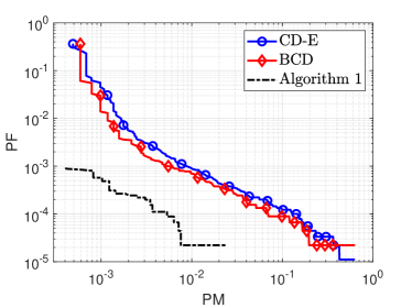
Figure 1: PM-PF trade-offs achieved by different centralized algorithms.

We further compare these centralized algorithms under different maximum delays and different numbers of APs. Due to the trade-off between PM and PF, we show the probability of error when PF $=$ PM by appropriately setting the threshold $\gamma$. The probability of error versus the maximum delay $T$ is shown in Fig. 2(a), where the numbers of APs and antennas at each AP are set as $M=N=8$ and the length of the effective signature sequences is fixed as $L+T=10$. In particular, $(L=10,~{}T=0)$ represents ideal synchronous transmissions with no delay. It can be seen that while all the approaches result in higher PM as $T$ increases up to $8$, Algorithm 1 always performs the best, which demonstrates the superiority of Algorithm 1 under asynchronous transmissions.

On the other hand, the probability of error versus the number of APs $M$ is shown in Fig. 2(b), where the length of the signature sequences and the maximum delay are set as $L=9$ and $T=1$, respectively. The total number of antennas at all the APs is fixed as $MN=64$. It can be seen that as $M$ increases from $1$ to $16$, the detection performance of all the approaches becomes better. This performance improvement comes from the fact that when there are more APs in the area, the distance between each device and each AP becomes shorter, resulting in a higher SNR at each AP. On the other hand, when $M$ further increases, the antenna number at each AP $N$ becomes much smaller. The significant decrease in the spatial resolution makes the detection performance worse. Nevertheless, we can see that Algorithm 1 always performs better than the other two approaches in the whole range of $M$.

To demonstrate the superiority of massive MIMO, we further show the performance comparison under different numbers of antennas in Fig. 2(c). We fix the number of APs as $M=8$ and vary the number of antennas at each AP such that the total number of antennas increases from $32$ to $96$. It can be seen that while the detection performance of all the approaches becomes better as the number of antennas increases, the proposed Algorithm 1 always achieves the best performance. Due to the superiority of Algorithm 1, we adopt it as a baseline for the proposed distributed algorithms in the rest of simulations.

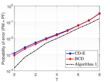
(a) Probability of error versus $T$.

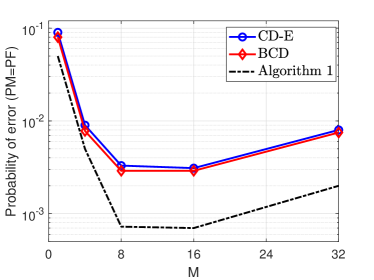
(b) Probability of error versus $M$.

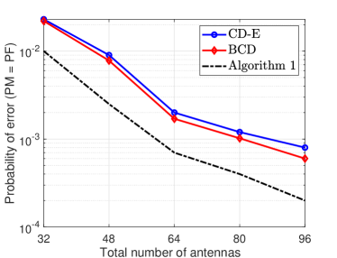
(c) Probability of error versus total number of antennas.

Figure 2: Performance comparison of centralized algorithms.

VI-C Proposed Distributed Algorithms Versus Centralized Algorithm

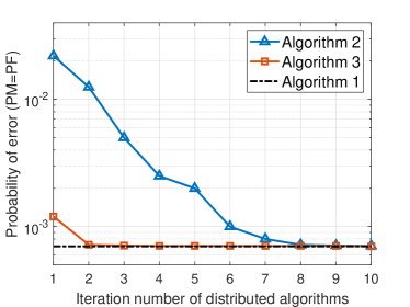
(a) Probability of error versus iteration number $I$.

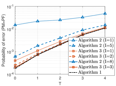
(b) Probability of error versus $T$.

Figure 3: Performance comparison of distributed algorithms.

Next, we show the detection performance of the proposed distributed Algorithm 2 and Algorithm 3, and compare them to that of the centralized algorithm. The probability of error versus the iteration number of the distributed algorithms is shown in Fig. 3(a), where $M=N=8$, $L=9$, and $T=1$. For fair comparison, all these algorithms are executed under ideal fronthauls. It can be seen that both Algorithm 2 and Algorithm 3 achieve fast convergence (within $8$ iterations) to the result of Algorithm 1. Furthermore, Fig. 3(b) shows that pretty fast convergence can be achieved under different $T$. This means that Algorithm 2 or Algorithm 3 can replace Algorithm 1 without changing the performance. On the other hand, since Algorithm 3 is judiciously designed based on Algorithm 2, we can see that Algorithm 3 achieves an impressively fast convergence within only $2$ to $3$ iterations. As Algorithm 3 achieves the same performance to that of Algorithm 2 but with much faster convergence, we only show the performance of Algorithm 3 under capacity-limited fronthauls in the following simulations.

VI-D Performance Under Capacity-Limited Fronthauls

Next, we show how many quantization bits are needed to approach the results under ideal fronthauls. For the illustration purpose, we adopt a uniform scalar quantizer in Algorithm 1 and Algorithm 3, respectively. The probability of error versus $T$ is shown in Fig. 4(a), where $M=N=8$ and $L+T=10$. It can be seen that under different $T$, Algorithm 3 always performs very close to Algorithm 1. However, Algorithm 1 requires at least $16$ quantization bits per real-valued scalar to approach the performance under ideal fronthauls. When $14$ quantization bits are used, Algorithm 1 performs even worse than Algorithm 3 with only $4$ quantization bits and $I=1$ iteration. In Fig. 4(b), we show the probability of error versus $M$, where $L=9$, $T=1$, and $MN=64$. Similar to Fig. 4(a), we can see that under different $M$, Algorithm 3 always requires much fewer quantization bits per real-valued scalar to approach the detection performance under ideal fronthauls.

To clearly see the overall communication overheads, we analyze the number of bits required to be transmitted in Algorithm 1 and Algorithm 3 as follows. In Algorithm 1, the received signal $\mathbf{Y}_{m}$ is used via $\mathbf{Y}_{m}\mathbf{Y}_{m}^{\mathrm{H}}/N$, which is a Hermitian matrix with $(L+T)^{2}$ real-valued scalars. Thus, when $L+T\leq 2N$, each AP $m$ can quantize and send $\mathbf{Y}_{m}\mathbf{Y}_{m}^{\mathrm{H}}/N$ instead of $\mathbf{Y}_{m}$ (with $2(L+T)N$ real-valued scalars) to the CPU. With $Q_{1}$ denoting the number of quantization bits per real-valued scalar, the overall number of bits required by Algorithm 1 is $MQ_{1}(L+T)^{2}$ when $L+T\leq 2N$ or $2MQ_{1}(L+T)N$ otherwise. On the other hand, in Algorithm 3, each AP $m$ sends its quantized local detection result to the CPU at each iteration. With $Q_{2}$ denoting the number of quantization bits per real-valued scalar, the number of bits sent from each AP $m$ to the CPU is $Q_{2}K(T+1)$. Similarly, after the CPU updates $\mathbf{b}^{(i)}$, the number of bits sent from the CPU to each AP $m$ is also $Q_{2}K(T+1)$. Since Algorithm 3 can stop before sending $\mathbf{b}^{(I)}$ to the APs at the last iteration, the overall number of bits required by Algorithm 3 is $(2I-1)MKQ_{2}(T+1)$. For example, when $M=N=8$, $L=9$, $T=1$, $I=1$, $Q_{1}=14$, and $Q_{2}=4$, Algorithm 1 and Algorithm 3 require $11200$ and $6400$ quantization bits, respectively. This shows that even under the uniform scalar quantization, Algorithm 3 reduces the number of bits transmitted significantly.

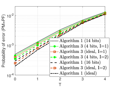
(a) Probability of error versus $T$.

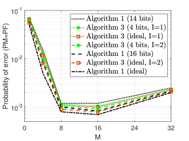
(b) Probability of error versus $M$.

Figure 4: Performance comparison between Algorithm 1 and Algorithm 3 using the simple uniform scalar quantization.

Since most of the local detection results are zero, the actual number of bits to be transmitted can be further reduced by using various data compression schemes. As a demonstration, we compare the total number of bits required by Algorithm 1 and Algorithm 3 using Huffman coding. In particular, Huffman coding is applied to the quantized contents for both Algorithm 1 and Algorithm 3. Figure 5 shows the simulation results for $M=N=8$, $L=9$, and $T=1$. For Algorithm 1, we consider different quantization levels $2^{11}$, $2^{14}$, and $2^{16}$, whereas for Algorithm 3, the quantization level is fixed as $2^{4}$ and each AP transmits the local detection results of $50$, $70$, $80$, and $100$ devices with the largest large-scale fading coefficients. We can see that while Huffman coding is effective in reducing the overall number of bits for both Algorithm 1 and Algorithm 3, the compression ratio is higher in Algorithm 3 due to the sparse local detection results. For example, before using Huffman coding, the number of bits required by Algorithm 3 is almost $2$ times smaller than that of Algorithm 1, whereas after using Huffman coding, the number of bits required by Algorithm 3 is at least $3$ times smaller than that of Algorithm 1.

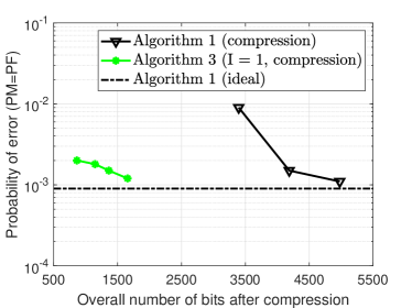
Figure 5: Probability of error versus overall number of bits after Huffman coding compression.

VII Conclusions

This paper studied asynchronous activity detection methods for cell-free massive MIMO. To tackle the discontinuous and nonconvex $\ell_{0}$-norm constraints due to the asynchronous transmissions, an equivalent reformulation of the original problem was established. A centralized algorithm and a distributed algorithm were proposed, with both being theoretically guaranteed to converge to a stationary point of the original asynchronous activity detection problem. Since the proposed algorithms address the $\ell_{0}$-norm constraints in a gentle fashion as the iteration number increases, the sequence generated by the proposed algorithms can get around bad stationary points caused by the highly nonconvex $\ell_{0}$-norm. To reduce the capacity requirements of the fronthauls in cell-free massive MIMO, a communication-efficient accelerated distributed algorithm was further designed. Simulation results demonstrated that the proposed centralized and distributed algorithms outperform state-of-the-art approaches, whereas the proposed accelerated distributed algorithm achieves a close detection performance to that of the centralized algorithm but with a much smaller number of bits to be transmitted on the fronthaul links.

Appendix A Proof of Theorem 1

We first prove that there exists a finite $\rho^{*}<\infty$ such that for any $\rho>\rho^{*}$, the stationary point of problem (8) is also a feasible point of problem (7). Let $\mathbf{b}^{*}$ denote a stationary point of problem (8), which satisfies the following first-order optimality condition[39]:

$$-\rho\sum_{k=1}^{K}\lim_{\tau\rightarrow 0^{+}}\frac{\max\limits_{t\in\{0,\ldots,T\}}\left(b_{k,t}^{*}+\tau{\color[rgb]{0,0,0}\tilde{d}}_{k,t}\right)-\max\limits_{t\in\{0,\ldots,T\}}b_{k,t}^{*}}{\tau}$$

$$+\sum_{m=1}^{M}\nabla f_{m}\left(\mathbf{b}^{*}\right)^{\mathrm{T}}{\color[rgb]{0,0,0}\tilde{\mathbf{d}}}+\rho\sum_{k=1}^{K}\sum_{t=0}^{T}{\color[rgb]{0,0,0}\tilde{d}}_{k,t}\geq 0,$$

$$\forall{\color[rgb]{0,0,0}\tilde{\mathbf{d}}}\in\mathcal{T}\left(\mathbf{b}^{*}\right),$$ (A.1)

where $f_{m}\left(\mathbf{b}\right)\triangleq\log|{\mathbf{C}}_{m}|+\text{Tr}\left({\mathbf{C}}_{m}^{-1}\mathbf{Y}_{m}\mathbf{Y}_{m}^{\mathrm{H}}\right){\color[rgb]{0,0,0}/N}$ and $\mathcal{T}\left(\mathbf{b}^{*}\right)$ is the tangent cone of the feasible set of problem (8) at $\mathbf{b}^{*}$. Denoting $\mathcal{W}(k)\triangleq\arg\max\limits_{t\in\{0,\ldots,T\}}b_{k,t}^{*}$, we have $\max\limits_{t\in\{0,\ldots,T\}}\left(b_{k,t}^{*}+\tau{\color[rgb]{0,0,0}\tilde{d}}_{k,t}\right)=\max\limits_{t\in\{0,\ldots,T\}}b_{k,t}^{*}+\tau\max\limits_{t\in\mathcal{W}(k)}\tilde{d}_{k,t},\forall\tau\rightarrow 0^{+}$. Using this equation and taking any $\omega(k)\in\arg\max\limits_{t\in\mathcal{W}(k)}\tilde{d}_{k,t}$ we can simplify (A) as

$$\sum_{m=1}^{M}\nabla f_{m}\left(\mathbf{b}^{*}\right)^{\mathrm{T}}{\color[rgb]{0,0,0}\tilde{\mathbf{d}}}+\rho\sum_{k=1}^{K}\left(\sum_{t=0}^{T}{\color[rgb]{0,0,0}\tilde{d}}_{k,t}-{\color[rgb]{0,0,0}\tilde{d}}_{k,\omega(k)}\right)\geq 0,$$

$$\forall{\color[rgb]{0,0,0}\tilde{\mathbf{d}}}\in\mathcal{T}\left(\mathbf{b}^{*}\right).$$ (A.2)

Notice that the first term of (A) can be upper bounded as

$$\sum_{m=1}^{M}\nabla f_{m}\left(\mathbf{b}^{*}\right)^{\mathrm{T}}{\color[rgb]{0,0,0}\tilde{\mathbf{d}}}\leq{\color[rgb]{0,0,0}\left\|\sum_{m=1}^{M}\nabla f_{m}\left(\mathbf{b}^{*}\right)\right\|_{\infty}\left\|{\color[rgb]{0,0,0}\tilde{\mathbf{d}}}\right\|_{1}}\triangleq\rho^{*}\left\|{\color[rgb]{0,0,0}\tilde{\mathbf{d}}}\right\|_{1},$$ (A.3)

where $\rho^{*}<\infty$ since $\mathbf{b}^{*}$ is bounded in $[0,1]^{K(T+1)}$. Substituting (A.3) into (A), we obtain

$$\rho^{*}\left\|{\color[rgb]{0,0,0}\tilde{\mathbf{d}}}\right\|_{1}+\rho\sum_{k=1}^{K}\left(\sum_{t=0}^{T}{\color[rgb]{0,0,0}\tilde{d}}_{k,t}-{\color[rgb]{0,0,0}\tilde{d}}_{k,\omega(k)}\right)\geq 0,~{}~{}\forall{\color[rgb]{0,0,0}\tilde{\mathbf{d}}}\in\mathcal{T}\left(\mathbf{b^{*}}\right).$$ (A.4)

Based on (A.4), we prove that when $\rho>\rho^{*}$, $\mathbf{b}^{*}$ must satisfy (LABEL:opt1c2) by contradiction. Suppose that (LABEL:opt1c2) does not hold, i.e., there exits $\bar{k}\in\left\{1,\ldots,K\right\}$ such that $\left\|\mathbf{b}_{\bar{k}}^{*}\right\|_{0}>1$. Moreover, since $\mathbf{b}^{*}\in[0,1]^{K(T+1)}$ in problem (8), there must exist one $\phi(\bar{k})\neq\omega(\bar{k})$ satisfying $b_{\bar{k},\phi(\bar{k})}^{*}>0$. On the other hand, notice that any ${\color[rgb]{0,0,0}\tilde{\mathbf{d}}}\in\mathcal{T}\left(\mathbf{b^{*}}\right)$ should satisfy

$$\begin{cases}{\color[rgb]{0,0,0}\tilde{d}}_{k,t}\geq 0,&\text{ if }b_{k,t}^{*}=0,\cr{\color[rgb]{0,0,0}\tilde{d}}_{k,t}\in\mathbb{R},&\text{ if }b_{k,t}^{*}\in(0,1),\cr{\color[rgb]{0,0,0}\tilde{d}}_{k,t}\leq 0,&\text{ if }b_{k,t}^{*}=1,\end{cases}~{}~{}\forall k=1,\ldots,K,~{}~{}\forall t=0,\ldots,T.$$ (A.5)

Consequently, there exists one ${\color[rgb]{0,0,0}\tilde{\mathbf{d}}}\in\mathcal{T}\left(\mathbf{b^{*}}\right)$ satisfying ${\color[rgb]{0,0,0}\tilde{d}}_{\bar{k},\phi(\bar{k})}=-1$ and ${\color[rgb]{0,0,0}\tilde{d}}_{k,t}=0,\forall(k,t)\neq(\bar{k},\phi(\bar{k}))$. Substituting this ${\color[rgb]{0,0,0}\tilde{\mathbf{d}}}$ into (A.4), we obtain $\rho^{*}-\rho\geq 0$, which is contradictory to $\rho>\rho^{*}$. Therefore, when $\rho>\rho^{*}$, $\mathbf{b}^{*}$ must satisfy (LABEL:opt1c2). Together with the fact that (7b) is already satisfied in problem (8), we can conclude that $\mathbf{b}^{*}$ is a feasible point of problem (7).

Next, we prove that $\mathbf{b}^{*}$ must also be a stationary point problem (7) when $\rho>\rho^{*}$. Since $\mathbf{b}^{*}$ has been proved to be feasible to problem (7), we have $\left\|\mathbf{b}_{k}^{*}\right\|_{0}\leq 1$. Moreover, with $\mathcal{P}\left(\mathbf{b^{*}}\right)$ denoting the tangent cone of the feasible set of problem (7) at $\mathbf{b^{*}}$, for any ${\color[rgb]{0,0,0}\tilde{\mathbf{d}}}\in\mathcal{P}\left(\mathbf{b^{*}}\right)$, we have $\left\|\mathbf{b}_{k}^{*}+\tau{\color[rgb]{0,0,0}\tilde{\mathbf{d}}}_{k}\right\|_{0}\leq 1,\forall\tau\rightarrow 0^{+},\forall k=1,\ldots,K$. Consequently, we have $\sum\limits_{t=0}^{T}\left(b_{k,t}^{*}+\tau\tilde{d}_{k,t}\right)=\max\limits_{t\in\{0,\ldots,T\}}\left(b_{k,t}^{*}+\tau\tilde{d}_{k,t}\right),\forall\tau\rightarrow 0^{+}$. If $\left\|\mathbf{b}_{k}^{*}\right\|_{0}=0$, it reduces to $\sum\limits_{t=0}^{T}{\color[rgb]{0,0,0}\tilde{d}}_{k,t}=\tilde{d}_{k,\omega(k)}$. If $\left\|\mathbf{b}_{k}^{*}\right\|_{0}=1$, from $\left\|\mathbf{b}_{k}^{*}+\tau{\color[rgb]{0,0,0}\tilde{\mathbf{d}}}_{k}\right\|_{0}\leq 1$, we have $\tilde{d}_{k,t}=0,\forall t\neq\omega(k)$. Thus, it also follows that $\sum\limits_{t=0}^{T}{\color[rgb]{0,0,0}\tilde{d}}_{k,t}=\tilde{d}_{k,\omega(k)}$. On the other hand, since the feasible set of (7) is a subset of the feasible set of (8), we have $\mathcal{P}\left(\mathbf{b^{*}}\right)\subseteq\mathcal{T}\left(\mathbf{b^{*}}\right)$. Substituting $\sum\limits_{t=0}^{T}{\color[rgb]{0,0,0}\tilde{d}}_{k,t}=\tilde{d}_{k,\omega(k)}$ into (A) and focusing on ${\color[rgb]{0,0,0}\tilde{\mathbf{d}}}\in\mathcal{P}\left(\mathbf{b^{*}}\right)$ give

$$\sum_{m=1}^{M}\nabla f_{m}\left(\mathbf{b}^{*}\right)^{\mathrm{T}}{\color[rgb]{0,0,0}\tilde{\mathbf{d}}}\geq 0,~{}~{}\forall{\color[rgb]{0,0,0}\tilde{\mathbf{d}}}\in\mathcal{P}\left(\mathbf{b^{*}}\right),$$ (A.6)

which means that $\mathbf{b^{*}}$ is also a stationary point of problem (7).

Finally, we prove that the global optimal solutions of the two problems are identical. Let $\mathbf{b}^{*}$ denote the global optimal solution of problem (8). Let $F(\cdot)$ and $\mathbf{b}^{\star}$ denote the cost function and the optimal solution of problem (7), respectively. Since both $\mathbf{b}^{*}$ and $\mathbf{b}^{\star}$ are feasible to problem (7), we have $\left\|\mathbf{b}_{k}^{*}\right\|_{0}\leq 1$ and $\left\|\mathbf{b}_{k}^{\star}\right\|_{0}\leq 1$. Consequently, we have $\sum\limits_{t=0}^{T}b_{k,t}^{*}=\max\limits_{t\in\{0,\ldots,T\}}b_{k,t}^{*}$ and $\sum\limits_{t=0}^{T}b_{k,t}^{\star}=\max\limits_{t\in\{0,\ldots,T\}}b_{k,t}^{\star}$. With $G(\cdot)$ denoting the cost function of problem (8), by substituting the above two equalities into $G\left(\mathbf{b}^{*}\right)$ and $G\left(\mathbf{b}^{\star}\right)$, we have $F\left(\mathbf{b}^{*}\right)=G\left(\mathbf{b}^{*}\right)$ and $G\left(\mathbf{b}^{\star}\right)=F\left(\mathbf{b}^{\star}\right)$. Moreover, since $\mathbf{b}^{*}$ is the optimal solution of problem (8), we have $F\left(\mathbf{b}^{*}\right)=G\left(\mathbf{b}^{*}\right)\leq G\left(\mathbf{b}^{\star}\right)=F\left(\mathbf{b}^{\star}\right)$. On the other hand, since $\mathbf{b}^{*}$ is a feasible point of problem (7), we also have $F\left(\mathbf{b}^{*}\right)\geq F\left(\mathbf{b}^{\star}\right)$. Combining the above two inequalities, we finally have $F\left(\mathbf{b}^{*}\right)=G\left(\mathbf{b}^{*}\right)=G\left(\mathbf{b}^{\star}\right)=F\left(\mathbf{b}^{\star}\right)$, which means that optimal solutions of problems (7) and (8) are identical.

Appendix B Proof of Proposition 1

Problem (9) can be decomposed into $K$ subproblems, with each written as

$$\mathbf{b}_{k}^{(i)}=\arg\min_{\mathbf{b}_{k}\in[0,1]^{T+1}}\sum_{t=0}^{T}\left(b_{k,t}-\alpha_{k,t}^{(i)}\right)^{2}-2\eta_{i}\rho\max_{t\in\{0,\ldots,T\}}b_{k,t},$$ (B.1)

where $\alpha_{k,t}^{(i)}\triangleq b_{k,t}^{(i-1)}-\eta_{i}d_{k,t}^{(i-1)}$. Taking any $\omega(k)\in\arg\max\limits_{t\in\{0,\ldots,T\}}b_{k,t}^{(i)}$, problem (B.1) can be equivalently written as

$$b_{k,t}^{(i)}=\begin{cases}\arg\min\limits_{b_{k,t}\in[0,1]}\left(b_{k,t}-\alpha_{k,t}^{(i)}\right)^{2}-2\eta_{i}\rho b_{k,t},&\text{if }t=\omega(k),\cr\arg\min\limits_{b_{k,t}\in[0,1]}\left(b_{k,t}-\alpha_{k,t}^{(i)}\right)^{2},&\text{otherwise},\end{cases}$$ (B.2)

which can be simplified as

$$b_{k,t}^{(i)}=\begin{cases}{\color[rgb]{0,0,0}\Pi_{[0,1]}}\left(\alpha_{k,t}^{(i)}+\eta_{i}\rho\right),&\text{if }t=\omega(k),\cr{\color[rgb]{0,0,0}\Pi_{[0,1]}}\left(\alpha_{k,t}^{(i)}\right),&\text{otherwise}.\end{cases}$$ (B.3)

However, since $\omega(k)$ is defined based on the solution $\mathbf{b}_{k}^{(i)}$ itself, (B.3) cannot be directly used as the closed-form solution. Next, we prove that $\omega(k)$ can be replaced by $\tau(k)\in\arg\max\limits_{t\in\{0,\ldots,T\}}\alpha_{k,t}^{(i)}$. According to the definition of $\tau(k)$, we have $\alpha_{k,\tau(k)}^{(i)}\geq\alpha_{k,t}^{(i)},\forall t=0,\ldots,T$. Since $\eta_{i}\rho>0$ and ${\color[rgb]{0,0,0}\Pi_{[0,1]}}\left(\cdot\right)$ is a monotonically non-decreasing function, we have

$${\color[rgb]{0,0,0}\Pi_{[0,1]}}\left(\alpha_{k,\tau(k)}^{(i)}+\eta_{i}\rho\right)\geq{\color[rgb]{0,0,0}\Pi_{[0,1]}}\left(\alpha_{k,t}^{(i)}\right),~{}~{}\forall t=0,\ldots,T.$$ (B.4)

On the other hand, from (B.3), we also have

$$b_{k,\omega(k)}^{(i)}={\color[rgb]{0,0,0}\Pi_{[0,1]}}\left(\alpha_{k,\omega(k)}^{(i)}+\eta_{i}\rho\right)\geq{\color[rgb]{0,0,0}\Pi_{[0,1]}}\left(\alpha_{k,t}^{(i)}\right)=b_{k,t}^{(i)},$$

$$\forall t=0,\ldots,T.~{}~{}$$ (B.5)

Comparing (B.4) and (B), we can conclude that $\omega(k)$ in (B.3) can be replaced by $\tau(k)$, and the optimal solution of (9) is given by (1).

Appendix C Proof of Theorem 2

Denote the cost function of problems (8) and (9) as $G\left(\mathbf{b}\right)=G_{0}\left(\mathbf{b}\right)-\rho\sum\limits_{k=1}^{K}\max\limits_{t\in\{0,\ldots,T\}}b_{k,t}$ and $U\left(\mathbf{b}\right)$, respectively. Taking the second-order Taylor expansion to $G_{0}\left(\mathbf{b}\right)$ at $\mathbf{b}^{(i-1)}$, we have (C.1),

$$G\left(\mathbf{b}\right) \leq \underbrace{G_{0}\left(\mathbf{b}^{(i-1)}\right)+\left(\mathbf{d}^{(i-1)}\right)^{\mathrm{T}}\left(\mathbf{b}-\mathbf{b}^{(i-1)}\right)+\frac{L_{\text{d}}}{2}\left\|\mathbf{b}-\mathbf{b}^{(i-1)}\right\|_{2}^{2}-\rho\sum_{k=1}^{K}\max_{t\in\{0,\ldots,T\}}b_{k,t}}_{U_{1}(\mathbf{b})},$$ (C.1)

$$\leq \underbrace{G_{0}\left(\mathbf{b}^{(i-1)}\right)+\left(\mathbf{d}^{(i-1)}\right)^{\mathrm{T}}\left(\mathbf{b}-\mathbf{b}^{(i-1)}\right)+\frac{1}{2\eta_{i}}\left\|\mathbf{b}-\mathbf{b}^{(i-1)}\right\|_{2}^{2}-\rho\sum_{k=1}^{K}\max_{t\in\{0,\ldots,T\}}b_{k,t}}_{U_{2}\left(\mathbf{b}\right)},$$

$$= U\left(\mathbf{b}\right)+C_{0}^{(i-1)},~{}~{}\forall\mathbf{b}\in[0,1]^{K(T+1)},$$

where $\mathbf{d}^{(i-1)}\triangleq\nabla G_{0}\left(\mathbf{b}^{(i-1)}\right)$, $L_{\text{d}}$ is the Lipschitz constant of $\nabla G_{0}\left(\mathbf{b}\right)$, and $C_{0}^{(i-1)}\triangleq G_{0}\left(\mathbf{b}^{(i-1)}\right)-\eta_{i}\left\|\mathbf{d}^{(i-1)}\right\|_{2}^{2}/2$. The first inequality in (C.1) is due to the fact that $\nabla G_{0}(\mathbf{b})$ is Lipschitz continuous with constant $L_{\text{d}}$ and the second inequality comes from $\eta_{i}<1/L_{\text{d}}$. Consequently, we have

$$G\left(\mathbf{b}^{(i-1)}\right)-G\left(\mathbf{b}^{(i)}\right)$$ (C.2)

$$\geq G\left(\mathbf{b}^{(i-1)}\right)-U_{1}\left(\mathbf{b}^{(i)}\right)=U_{2}\left(\mathbf{b}^{(i-1)}\right)-U_{1}\left(\mathbf{b}^{(i)}\right)$$

$$\geq U_{2}\left(\mathbf{b}^{(i)}\right)-U_{1}\left(\mathbf{b}^{(i)}\right)$$

$$= \left(\frac{1}{2\eta_{i}}-\frac{L_{\text{d}}}{2}\right)\left\|\mathbf{b}^{(i)}-\mathbf{b}^{(i-1)}\right\|_{2}^{2}\geq 0,$$

where the second inequality is because $\mathbf{b}^{(i)}$ is the optimal solution of problem (9) and hence also the minimizer of $U_{2}\left(\mathbf{b}\right)$. Summing (C.2) over $i$ yields

$$\sum_{i=1}^{\infty}\left(\frac{1}{2\eta_{i}}-\frac{L_{\text{d}}}{2}\right)\left\|\mathbf{b}^{(i)}-\mathbf{b}^{(i-1)}\right\|_{2}^{2}$$ (C.3)

$$\leq G\left(\mathbf{b}^{(0)}\right)-G\left(\mathbf{b}^{(\infty)}\right)<\infty,$$

where the second inequaltiy is becasue $G\left(\mathbf{b}\right)$ is bounded below by $\sum_{m=1}^{M}(L+T)\log\sigma_{m}^{2}$. Since ${1}/{(2\eta_{i})}-{L_{\text{d}}}/{2}>0$, (C.3) yields $\lim\limits_{i\rightarrow\infty}\left\|\mathbf{b}^{(i)}-\mathbf{b}^{(i-1)}\right\|_{2}=0$. Thus, with $\mathbf{b}^{*}$ denoting a limit point of $\mathbf{b}^{(i)}$, we also have $\mathbf{b}^{(i-1)}\rightarrow\mathbf{b}^{*}$. Letting $i\rightarrow\infty$ in (9), we obtain (C.4),

$$\mathbf{b}^{*} = \arg\min_{\mathbf{b}\in[0,1]^{K(T+1)}}\frac{1}{2\eta_{*}}\left\|\mathbf{b}-\left(\mathbf{b}^{*}-{\color[rgb]{0,0,0}\eta_{*}}\mathbf{d}^{*}\right)\right\|_{2}^{2}-\rho\sum_{k=1}^{K}\max_{t\in\{0,\ldots,T\}}b_{k,t},$$ (C.4)

$$= \arg\min_{\mathbf{b}\in[0,1]^{K(T+1)}}G_{0}\left(\mathbf{b}^{*}\right)+\left(\mathbf{d}^{*}\right)^{\mathrm{T}}\left(\mathbf{b}-\mathbf{b}^{*}\right)+\frac{1}{2\eta_{*}}\left\|\mathbf{b}-\mathbf{b}^{*}\right\|_{2}^{2}-\rho\sum_{k=1}^{K}\max_{t\in\{0,\ldots,T\}}b_{k,t},~{}~{}$$

where $\eta_{*}>0$ is the limit point of $\eta_{i}$ and the second equality comes from the last equality in (C.1). Since $\mathbf{b}^{*}$ is the optimal solution of (C.4), we have

$$\left(\mathbf{d}^{*}\right)^{\mathrm{T}}\left(\mathbf{b}-\mathbf{b}^{*}\right)+\frac{1}{2\eta_{*}}\left\|\mathbf{b}-\mathbf{b}^{*}\right\|_{2}^{2}-\rho\sum_{k=1}^{K}\max_{t\in\{0,\ldots,T\}}b_{k,t}$$ (C.5)

$$\geq -\rho\sum_{k=1}^{K}\max_{t\in\{0,\ldots,T\}}b_{k,t}^{*},\forall\mathbf{b}\in[0,1]^{K(T+1)}.$$

Let $\mathcal{T}\left(\mathbf{b^{*}}\right)$ denote the tangent cone of $\mathbf{b}\in[0,1]^{K(T+1)}$ at $\mathbf{b}^{*}$. Substituting $\mathbf{b}=\mathbf{b}^{*}+\tau{\color[rgb]{0,0,0}\tilde{\mathbf{d}}}$ with ${\color[rgb]{0,0,0}\tilde{\mathbf{d}}}\in\mathcal{T}\left(\mathbf{b^{*}}\right)$ into (C.5) and dividing $\tau$ on both sides of (C.5), we have

$$-\rho\sum_{k=1}^{K}\lim_{\tau\rightarrow 0^{+}}\frac{\max\limits_{t\in\{0,\ldots,T\}}\left(b_{k,t}^{*}+\tau{\color[rgb]{0,0,0}\tilde{d}}_{k,t}\right)-\max\limits_{t\in\{0,\ldots,T\}}b_{k,t}^{*}}{\tau}$$

$$+\left(\mathbf{d}^{*}\right)^{\mathrm{T}}{\color[rgb]{0,0,0}\tilde{\mathbf{d}}}\geq 0,~{}~{}\forall{\color[rgb]{0,0,0}\tilde{\mathbf{d}}}\in\mathcal{T}\left(\mathbf{b^{*}}\right).$$ (C.6)

Noticing that $\mathbf{d}^{*}$ is the gradient of $G_{0}(\mathbf{b})$, we can rewrite (C) as (A), which means that the limit point $\mathbf{b^{*}}$ is a stationary point of problem (8).

Appendix D Proof of Theorem 3

We first show that $\mathcal{L}\left(\left\{\mathbf{x}_{m}^{(i)}\right\}_{m=1}^{M},\mathbf{b}^{(i)};\left\{\boldsymbol{\lambda}_{m}^{(i)}\right\}_{m=1}^{M}\right)$ is monotonically decreasing as $i$ increases. With $U_{3}\left(\mathbf{b}\right)\triangleq\mathcal{L}\left(\left\{\mathbf{x}_{m}^{(i-1)}\right\}_{m=1}^{M},\mathbf{b};\left\{\boldsymbol{\lambda}_{m}^{(i-1)}\right\}_{m=1}^{M}\right)+{\delta}/{2}\left\|\mathbf{b}-\mathbf{b}^{(i-1)}\right\|_{2}^{2}$ and $U_{4}\left(\mathbf{b}\right)$ denoting the cost function of problem (IV), we have $\mathcal{L}\left(\left\{\mathbf{x}_{m}^{(i-1)}\right\}_{m=1}^{M},\mathbf{b};\left\{\boldsymbol{\lambda}_{m}^{(i-1)}\right\}_{m=1}^{M}\right)\leq U_{3}\left(\mathbf{b}\right)=U_{4}\left(\mathbf{b}\right)+\sum\limits_{m=1}^{M}f_{m}\left(\mathbf{x}_{m}^{(i-1)}\right)$, where the equality holds when $\mathbf{b}=\mathbf{b}^{(i-1)}$. Consequently,

$$\mathcal{L}\left(\left\{\mathbf{x}_{m}^{(i-1)}\right\}_{m=1}^{M},\mathbf{b}^{(i-1)};\left\{\boldsymbol{\lambda}_{m}^{(i-1)}\right\}_{m=1}^{M}\right)$$ (D.1)

$$-\mathcal{L}\left(\left\{\mathbf{x}_{m}^{(i-1)}\right\}_{m=1}^{M},\mathbf{b}^{(i)};\left\{\boldsymbol{\lambda}_{m}^{(i-1)}\right\}_{m=1}^{M}\right)$$

$$= U_{3}\left(\mathbf{b}^{(i-1)}\right)-\mathcal{L}\left(\left\{\mathbf{x}_{m}^{(i-1)}\right\}_{m=1}^{M},\mathbf{b}^{(i)};\left\{\boldsymbol{\lambda}_{m}^{(i-1)}\right\}_{m=1}^{M}\right)$$

$$\geq U_{3}\left(\mathbf{b}^{(i)}\right)-\mathcal{L}\left(\left\{\mathbf{x}_{m}^{(i-1)}\right\}_{m=1}^{M},\mathbf{b}^{(i)};\left\{\boldsymbol{\lambda}_{m}^{(i-1)}\right\}_{m=1}^{M}\right)$$

$$= \frac{\delta}{2}\left\|\mathbf{b}^{(i)}-\mathbf{b}^{(i-1)}\right\|_{2}^{2},$$

where the last inequality holds because $\mathbf{b}^{(i)}$ is the optimal solution of problem (IV), and hence also the minimizer of $U_{3}\left(\mathbf{b}\right)$.

On the other hand, since $\mu>2L_{m}$, we have $\mu\mathbf{I}_{K(T+1)}-\nabla^{2}f_{m}(\mathbf{x}_{m})\succeq L_{m}\mathbf{I}_{K(T+1)}$, which means that problem (17) is strongly convex with modulus $L_{m}$. Thus, line 6 of Algorithm 2 can solve problem (17) to the optimal solution $\mathbf{x}_{m}^{(i)}$ and we have

$$\mathcal{L}\left(\left\{\mathbf{x}_{m}^{(i-1)}\right\}_{m=1}^{M},\mathbf{b}^{(i)};\left\{\boldsymbol{\lambda}_{m}^{(i-1)}\right\}_{m=1}^{M}\right)$$ (D.2)

$$-\mathcal{L}\left(\left\{\mathbf{x}_{m}^{(i)}\right\}_{m=1}^{M},\mathbf{b}^{(i)};\left\{\boldsymbol{\lambda}_{m}^{(i-1)}\right\}_{m=1}^{M}\right)$$

$$\geq \sum_{m=1}^{M}\frac{L_{m}}{2}\left\|\mathbf{x}_{m}^{(i)}-\mathbf{x}_{m}^{(i-1)}\right\|_{2}^{2}.$$

Moreover, since $\mathbf{x}_{m}^{(i)}$ is the optimal solution of problem (17), we have

$$\nabla f_{m}\left(\mathbf{x}_{m}^{(i)}\right)+\boldsymbol{\lambda}_{m}^{(i-1)}+{\mu}\left(\mathbf{x}_{m}^{(i)}-\mathbf{b}^{(i)}\right)=\mathbf{0},~{}~{}\forall m=1,\ldots,M.$$ (D.3)

Substituting (20) into (D.3), we obtain

$$\left\|\boldsymbol{\lambda}_{m}^{(i-1)}-\boldsymbol{\lambda}_{m}^{(i)}\right\|_{2} = \left\|\nabla f_{m}\left(\mathbf{x}_{m}^{(i-1)}\right)-\nabla f_{m}\left(\mathbf{x}_{m}^{(i)}\right)\right\|_{2}$$ (D.4)

$$\leq L_{m}\left\|\mathbf{x}_{m}^{(i-1)}-\mathbf{x}_{m}^{(i)}\right\|_{2}.$$

Consequently, we have

$$\mathcal{L}\left(\left\{\mathbf{x}_{m}^{(i)}\right\}_{m=1}^{M},\mathbf{b}^{(i)};\left\{\boldsymbol{\lambda}_{m}^{(i-1)}\right\}_{m=1}^{M}\right)$$ (D.5)

$$-\mathcal{L}\left(\left\{\mathbf{x}_{m}^{(i)}\right\}_{m=1}^{M},\mathbf{b}^{(i)};\left\{\boldsymbol{\lambda}_{m}^{(i)}\right\}_{m=1}^{M}\right)$$

$$= \sum_{m=1}^{M}\left(\boldsymbol{\lambda}_{m}^{(i-1)}-\boldsymbol{\lambda}_{m}^{(i)}\right)^{\mathrm{T}}\left(\mathbf{x}_{m}^{(i)}-\mathbf{b}^{(i)}\right)$$

$$= -\frac{1}{\mu}\sum_{m=1}^{M}\left\|\boldsymbol{\lambda}_{m}^{(i-1)}-\boldsymbol{\lambda}_{m}^{(i)}\right\|_{2}^{2}$$

$$\geq -\frac{1}{\mu}\sum_{m=1}^{M}L_{m}^{2}\left\|\mathbf{x}_{m}^{(i-1)}-\mathbf{x}_{m}^{(i)}\right\|_{2}^{2},$$

where the second equality comes from (20) and the last inequality is due to (D.4). Combining (D.1), (D.2), and (D.5), we obtain

$$\mathcal{L}\left(\left\{\mathbf{x}_{m}^{(i-1)}\right\}_{m=1}^{M},\mathbf{b}^{(i-1)};\left\{\boldsymbol{\lambda}_{m}^{(i-1)}\right\}_{m=1}^{M}\right)$$ (D.6)

$$-\mathcal{L}\left(\left\{\mathbf{x}_{m}^{(i)}\right\}_{m=1}^{M},\mathbf{b}^{(i)};\left\{\boldsymbol{\lambda}_{m}^{(i)}\right\}_{m=1}^{M}\right)$$

$$\geq \sum_{m=1}^{M}\left(\frac{L_{m}}{2}-\frac{L_{m}^{2}}{\mu}\right)\left\|\mathbf{x}_{m}^{(i)}-\mathbf{x}_{m}^{(i-1)}\right\|_{2}^{2}$$

$$+\frac{\delta}{2}\left\|\mathbf{b}^{(i)}-\mathbf{b}^{(i-1)}\right\|_{2}^{2}\geq 0,$$

where the last inequality is due to $\mu>2L_{m}$ and $\delta>0$. Therefore, $\mathcal{L}\left(\left\{\mathbf{x}_{m}^{(i)}\right\}_{m=1}^{M},\mathbf{b}^{(i)};\left\{\boldsymbol{\lambda}_{m}^{(i)}\right\}_{m=1}^{M}\right)$ is monotonically decreasing.

Next, we prove that $\mathcal{L}\left(\left\{\mathbf{x}_{m}^{(i)}\right\}_{m=1}^{M},\mathbf{b}^{(i)};\left\{\boldsymbol{\lambda}_{m}^{(i)}\right\}_{m=1}^{M}\right)$ is lower bounded. Substituting (20) into (D.3), we have $\boldsymbol{\lambda}_{m}^{(i)}=-\nabla f_{m}\left(\mathbf{x}_{m}^{(i)}\right)$. Substituting this equation into (14), we obtain

$$\mathcal{L}\left(\left\{\mathbf{x}_{m}^{(i)}\right\}_{m=1}^{M},\mathbf{b}^{(i)};\left\{\boldsymbol{\lambda}_{m}^{(i)}\right\}_{m=1}^{M}\right)$$ (D.7)

$$= \sum_{m=1}^{M}f_{m}\left(\mathbf{x}_{m}^{(i)}\right)+\rho\sum_{k=1}^{K}\left(\sum_{t=0}^{T}b_{k,t}^{(i)}-\max_{t\in\{0,\ldots,T\}}b_{k,t}^{(i)}\right)$$

$$+\sum_{m=1}^{M}\nabla f_{m}\left(\mathbf{x}_{m}^{(i)}\right)^{\mathrm{T}}\left(\mathbf{b}^{(i)}-\mathbf{x}_{m}^{(i)}\right)$$

$$+\frac{\mu}{2}\sum_{m=1}^{M}\left\|\mathbf{x}_{m}^{(i)}-\mathbf{b}^{(i)}\right\|_{2}^{2}.$$

Since $\mu\mathbf{I}_{K(T+1)}\succeq L_{m}\mathbf{I}_{K(T+1)}\succeq\nabla^{2}f_{m}\left(\mathbf{x}_{m}\right)$, we have

$$\sum_{m=1}^{M}f_{m}\left(\mathbf{x}_{m}^{(i)}\right)+\sum_{m=1}^{M}\nabla f_{m}\left(\mathbf{x}_{m}^{(i)}\right)^{\mathrm{T}}\left(\mathbf{b}^{(i)}-\mathbf{x}_{m}^{(i)}\right)$$

$$+\frac{\mu}{2}\sum_{m=1}^{M}\left\|\mathbf{x}_{m}^{(i)}-\mathbf{b}^{(i)}\right\|_{2}^{2}\geq\sum_{m=1}^{M}f_{m}\left(\mathbf{b}^{(i)}\right).$$ (D.8)

Substituting (D) into (D.7), we obtain

$$\mathcal{L}\left(\left\{\mathbf{x}_{m}^{(i)}\right\}_{m=1}^{M},\mathbf{b}^{(i)};\left\{\boldsymbol{\lambda}_{m}^{(i)}\right\}_{m=1}^{M}\right)$$ (D.9)

$$\geq \sum_{m=1}^{M}f_{m}\left(\mathbf{b}^{(i)}\right)+\rho\sum_{k=1}^{K}\left(\sum_{t=0}^{T}b_{k,t}^{(i)}-\max_{t\in\{0,\ldots,T\}}b_{k,t}^{(i)}\right)$$

$$\geq \sum_{m=1}^{M}(L+T)\log\sigma_{m}^{2},$$

which means that $\mathcal{L}\left(\left\{\mathbf{x}_{m}^{(i)}\right\}_{m=1}^{M},\mathbf{b}^{(i)};\left\{\boldsymbol{\lambda}_{m}^{(i)}\right\}_{m=1}^{M}\right)$ is lower bounded.

Finally, we prove that any limit point of the sequence $\left(\left\{\mathbf{x}_{m}^{(i)}\right\}_{m=1}^{M},\mathbf{b}^{(i)};\left\{\boldsymbol{\lambda}_{m}^{(i)}\right\}_{m=1}^{M}\right)$ is a stationary point of problem (13). Summing (D.6) over $i$ yields

$$\sum_{i=1}^{\infty}\frac{\delta}{2}\left\|\mathbf{b}^{(i)}-\mathbf{b}^{(i-1)}\right\|_{2}^{2}$$

$$+\sum_{i=1}^{\infty}\sum_{m=1}^{M}\left(\frac{L_{m}}{2}-\frac{L_{m}^{2}}{\mu}\right)\left\|\mathbf{x}_{m}^{(i)}-\mathbf{x}_{m}^{(i-1)}\right\|_{2}^{2}$$

$$\leq \mathcal{L}\left(\left\{\mathbf{x}_{m}^{(0)}\right\}_{m=1}^{M},\mathbf{b}^{(0)};\left\{\boldsymbol{\lambda}_{m}^{(0)}\right\}_{m=1}^{M}\right)$$

$$-\mathcal{L}\left(\left\{\mathbf{x}_{m}^{(\infty)}\right\}_{m=1}^{M},\mathbf{b}^{(\infty)};\left\{\boldsymbol{\lambda}_{m}^{(\infty)}\right\}_{m=1}^{M}\right)<\infty,$$

where the second inequality comes from (D.9). Since $\mu>2L_{m}$ and $\delta>0$, (D) yields $\lim\limits_{i\rightarrow\infty}\left\|\mathbf{b}^{(i)}-\mathbf{b}^{(i-1)}\right\|_{2}=\lim\limits_{i\rightarrow\infty}\left\|\mathbf{x}_{m}^{(i)}-\mathbf{x}_{m}^{(i-1)}\right\|_{2}=0$. Together with (D.4) and (20), we also have $\lim\limits_{i\rightarrow\infty}\left\|{\color[rgb]{0,0,0}\boldsymbol{\lambda}_{m}^{(i)}-\boldsymbol{\lambda}_{m}^{(i-1)}}\right\|_{2}=\lim\limits_{i\rightarrow\infty}\left\|\mathbf{x}_{m}^{(i)}-\mathbf{b}^{(i)}\right\|_{2}=0$. Thus, with $\left(\left\{\mathbf{x}_{m}^{*}\right\}_{m=1}^{M},\mathbf{b}^{*};\left\{\boldsymbol{\lambda}_{m}^{*}\right\}_{m=1}^{M}\right)$ denoting a limit point of the sequence $\left(\left\{\mathbf{x}_{m}^{(i)}\right\}_{m=1}^{M},\mathbf{b}^{(i)};\left\{\boldsymbol{\lambda}_{m}^{(i)}\right\}_{m=1}^{M}\right)$, we have

$$\mathbf{b}^{(i-1)}\rightarrow\mathbf{b}^{*},~{}~{}\mathbf{x}_{m}^{(i-1)}\rightarrow\mathbf{x}_{m}^{*},~{}~{}\boldsymbol{\lambda}_{m}^{(i-1)}\rightarrow\boldsymbol{\lambda}_{m}^{*},$$

$$\forall m=1,\ldots,M,$$ (D.11)

$$\mathbf{x}_{m}^{*}=\mathbf{b}^{*},~{}~{}\forall m=1,\ldots,M.$$ (D.12)

Taking limit for (D.3), and using (D) and (D.12), we have

$$\nabla f_{m}\left(\mathbf{x}_{m}^{*}\right)+\boldsymbol{\lambda}_{m}^{*}=\mathbf{0},~{}~{}\forall m=1,\ldots,M.$$ (D.13)

On the other hand, since $\mathbf{b}^{(i)}$ is the optimal solution of problem (IV), it satisfies the following first-order optimality condition:

$$\rho\sum_{k=1}^{K}\sum_{t=0}^{T}{\color[rgb]{0,0,0}\tilde{d}}_{k,t}-\sum_{m=1}^{M}\left(\boldsymbol{\lambda}_{m}^{(i-1)}\right)^{\mathrm{T}}{\color[rgb]{0,0,0}\tilde{\mathbf{d}}}$$

$$-\rho\sum_{k=1}^{K}\lim_{\tau\rightarrow 0^{+}}\frac{\max\limits_{t\in\{0,\ldots,T\}}\left(b_{k,t}^{(i)}+\tau{\color[rgb]{0,0,0}\tilde{d}}_{k,t}\right)-\max\limits_{t\in\{0,\ldots,T\}}b_{k,t}^{(i)}}{\tau}$$

$$+\delta\left(\mathbf{b}^{(i)}-\mathbf{b}^{(i-1)}\right)^{\mathrm{T}}{\color[rgb]{0,0,0}\tilde{\mathbf{d}}}+\mu\sum_{m=1}^{M}\left(\mathbf{b}^{(i)}-\mathbf{x}_{m}^{(i-1)}\right)^{\mathrm{T}}{\color[rgb]{0,0,0}\tilde{\mathbf{d}}}\geq 0,$$

$$\forall{\color[rgb]{0,0,0}\tilde{\mathbf{d}}}\in\mathcal{T}\left(\mathbf{b}^{(i)}\right),$$ (D.14)

where $\mathcal{T}\left(\mathbf{b}^{(i)}\right)$ is the tangent cone of the feasible set of problem (IV) at $\mathbf{b}^{(i)}$. Taking limit for (D), using (D) and (D.12), and noticing that $\mathcal{T}\left(\mathbf{b}^{*}\right)\subseteq\mathcal{T}\left(\mathbf{b}^{i}\right)$ from (A.5), we have

$$\rho\sum_{k=1}^{K}\sum_{t=0}^{T}{\color[rgb]{0,0,0}\tilde{d}}_{k,t}-\sum_{m=1}^{M}\left(\boldsymbol{\lambda}_{m}^{*}\right)^{\mathrm{T}}{\color[rgb]{0,0,0}\tilde{\mathbf{d}}}$$ (D.15)

$$-\rho\sum_{k=1}^{K}\lim_{\tau\rightarrow 0^{+}}\frac{\max\limits_{t\in\{0,\ldots,T\}}\left(b_{k,t}^{*}+\tau{\color[rgb]{0,0,0}\tilde{d}}_{k,t}\right)-\max\limits_{t\in\{0,\ldots,T\}}b_{k,t}^{*}}{\tau}$$

$$\geq 0,~{}~{}\forall{\color[rgb]{0,0,0}\tilde{\mathbf{d}}}\in\mathcal{T}\left(\mathbf{b}^{*}\right).$$

Combining (D.12), (D.13), and (D.15), we can conclude that $\left(\left\{\mathbf{x}_{m}^{*}\right\}_{m=1}^{M},\mathbf{b}^{*};\left\{\boldsymbol{\lambda}_{m}^{*}\right\}_{m=1}^{M}\right)$ is a stationary point of problem (13).

References

• [1] C. Bockelmann, N. Pratas, H. Nikopour, K. Au, T. Svensson, C. Stefanovic, P. Popovski, and A. Dekorsy, “Massive machine-type communications in 5G: Physical and MAC-layer solutions,” IEEE Commun. Mag., vol. 54, no. 9, pp. 59–65, Sep. 2016.
• [2] L. Liu, E. G. Larsson, W. Yu, P. Popovski, Č. Stefanović, and E. de Carvalho, “Sparse signal processing for grant-free massive connectivity: A future paradigm for random access protocols in the internet of things,” IEEE Signal Process. Mag., vol. 35, no. 5, pp. 88–99, Sep. 2018.
• [3] X. Chen, D. W. K. Ng, W. Yu, E. G. Larsson, N. Al-Dhahir, and R. Schober, “Massive access for 5G and beyond,” IEEE J. Sel. Areas Commun., vol. 39, no. 3, pp. 615–637, Sep. 2021.
• [4] L. Liu and W. Yu, “Massive connectivity with massive MIMO-Part I: Device activity detection and channel estimation,” IEEE Trans. Signal Process., vol. 66, no. 11, pp. 2933–2946, Jun. 2018.
• [5] ——, “Massive connectivity with massive MIMO–Part II: Achievable rate characterization,” IEEE Trans. Signal Process., vol. 66, no. 11, pp. 2947–2959, Jun. 2018.
• [6] Z. Chen, F. Sohrabi, and W. Yu, “Sparse activity detection for massive connectivity,” IEEE Trans. Signal Process., vol. 66, no. 7, pp. 1890–1904, Apr. 2018.
• [7] T. Ding, X. Yuan, and S. C. Liew, “Sparsity learning-based multiuser detection in grant-free massive-device multiple access,” IEEE Trans. Wireless Commun., vol. 18, no. 7, pp. 3569–3582, Jul. 2019.
• [8] M. Ke, Z. Gao, Y. Wu, X. Gao, and R. Schober, “Compressive sensing-based adaptive active user detection and channel estimation: Massive access meets massive MIMO,” IEEE Trans. Signal Process., vol. 68, pp. 764–779, 2020.
• [9] Z. Chen, F. Sohrabi, and W. Yu, “Multi-cell sparse activity detection for massive random access: Massive MIMO versus cooperative MIMO,” IEEE Trans. Wireless Commun., vol. 18, no. 8, pp. 4060–4074, Aug. 2019.
• [10] K. Senel and E. G. Larsson, “Grant-free massive MTC-enabled massive MIMO: A compressive sensing approach,” IEEE Trans. Commun., vol. 66, no. 12, pp. 6164–6175, Dec. 2018.
• [11] W. Yuan, N. Wu, A. Zhang, X. Huang, Y. Li, and L. Hanzo, “Iterative receiver design for FTN signaling aided sparse code multiple access,” IEEE Trans. Wireless Commun., vol. 19, no. 2, pp. 915–928, Feb. 2020.
• [12] W. Yuan, N. Wu, Q. Guo, D. W. K. Ng, J. Yuan, and L. Hanzo, “Iterative joint channel estimation, user activity tracking, and data detection for FTN-NOMA systems supporting random access,” IEEE Trans. Commun., vol. 68, no. 5, pp. 2963–2977, May 2020.
• [13] S. Jiang, X. Yuan, X. Wang, C. Xu, and W. Yu, “Joint user identification, channel estimation, and signal detection for grant-free NOMA,” IEEE Trans. Wireless Commun., vol. 19, no. 10, pp. 6960–6976, Oct. 2020.
• [14] Y. Mei, Z. Gao, Y. Wu, W. Chen, J. Zhang, D. W. K. Ng, and M. Di Renzo, “Compressive sensing based joint activity and data detection for grant-free massive IoT access,” IEEE Trans. Wireless Commun., vol. 21, no. 3, pp. 1851–1869, Mar. 2022.
• [15] W. Chen, H. Xiao, L. Sun, and B. Ai, “Joint activity detection and channel estimation in massive MIMO systems with angular domain enhancement,” IEEE Trans. Wireless Commun., vol. 21, no. 5, pp. 2999–3011, May 2022.
• [16] X. Liu, Y. Shi, J. Zhang, and K. B. Letaief, “Massive CSI acquisition for dense cloud-RANs with spatial-temporal dynamics,” IEEE Trans. Wireless Commun., vol. 17, no. 4, pp. 2557–2570, Apr. 2018.
• [17] Q. He, T. Q. S. Quek, Z. Chen, Q. Zhang, and S. Li, “Compressive channel estimation and multi-user detection in C-RAN with low-complexity methods,” IEEE Trans. Wireless Commun., vol. 17, no. 6, pp. 3931–3944, Jun. 2018.
• [18] Y. Li, M. Xia, and Y.-C. Wu, “Activity detection for massive connectivity under frequency offsets via first-order algorithms,” IEEE Trans. Wireless Commun., vol. 18, no. 3, pp. 1988–2002, Mar. 2019.
• [19] X. Shao, X. Chen, and R. Jia, “A dimension reduction-based joint activity detection and channel estimation algorithm for massive access,” IEEE Trans. Signal Process., vol. 68, no. 1, pp. 420–435, Jan. 2020.
• [20] T. Li, J. Zhang, Z. Yang, Z. L. Yu, Z. Gu, and Y. Li, “Dynamic user activity and data detection for grant-free NOMA via weighted $\ell_{2,1}$ minimization,” IEEE Trans. Wireless Commun., vol. 21, no. 3, pp. 1638–1651, Mar. 2022.
• [21] S. Haghighatshoar, P. Jung, and G. Caire, “Improved scaling law for activity detection in massive MIMO systems,” in IEEE ISIT, 2018.
• [22] Z. Chen, F. Sohrabi, Y.-F. Liu, and W. Yu, “Covariance based joint activity and data detection for massive random access with massive MIMO,” in IEEE Int. Conf. Commun. (ICC), 2019.
• [23] Z. Wang, Z. Chen, Y.-F. Liu, F. Sohrab, and W. Yu, “An efficient active set algorithm for covariance based joint data and activity detection for massive random access with massive MIMO,” in IEEE International Conference on Acoustics, Speech and Signal Processing (ICASSP), 2021.
• [24] Z. Wang, Y.-F. Liu, Z. Chen, and W. Yu, “Accelerating coordinate descent via active set selection for device activity detection for multi-cell massive random access,” in IEEE International Workshop on Signal Processing Advances in Wireless Communications (SPAWC), 2021.
• [25] Z. Chen, F. Sohrabi, and W. Yu, “Sparse activity detection in multi-cell massive MIMO exploiting channel large-scale fading,” IEEE Trans. Signal Process., vol. 69, pp. 3768–3781, 2021.
• [26] Q. Lin, Y. Li, and Y.-C. Wu, “Sparsity constrained joint activity and data detection for massive access: A difference-of-norms penalty framework,” IEEE Trans. Wireless Commun., to appear 2022, doi:10.1109/TWC.2022.3204786.
• [27] A. Fengler, S. Haghighatshoar, P. Jung, and G. Caire, “Non-Bayesian activity detection, large-scale fading coefficient estimation, and unsourced random access with a massive MIMO receiver,” IEEE Trans. Inf. Theory, vol. 67, no. 5, pp. 2925–2951, May 2021.
• [28] Z. Chen, F. Sohrabi, Y.-F. Liu, and W. Yu, “Phase transition analysis for covariance based massive random access with massive MIMO,” IEEE Trans. Inf. Theory, vol. 68, no. 3, pp. 1696–1715, Mar. 2022.
• [29] M. Ke, Z. Gao, Y. Wu, X. Gao, and K.-K. Wong, “Massive access in cell-free massive MIMO-based internet of things: Cloud computing and edge computing paradigms,” IEEE J. Sel. Areas Commun., vol. 39, no. 3, pp. 756–772, Mar. 2021.
• [30] X. Shao, X. Chen, D. W. K. Ng, C. Zhong, and Z. Zhang, “Cooperative activity detection: Sourced and unsourced massive random access paradigms,” IEEE Trans. Signal Process., vol. 68, pp. 6578–6593, 2020.
• [31] U. K. Ganesan, E. Björnson, and E. G. Larsson, “Clustering based activity detection algorithms for grant-free random access in cell-free massive MIMO,” IEEE Trans. Commun., vol. 69, no. 11, pp. 7520–7530, Nov. 2021.
• [32] Y.-C. Wu, Q. Chaudhari, and E. Serpedin, “Clock synchronization of wireless sensor networks,” IEEE Signal Process. Mag., vol. 28, no. 1, pp. 124–138, Jan. 2011.
• [33] J. Du and Y.-C. Wu, “Distributed clock skew and offset estimation in wireless sensor networks: Asynchronous algorithm and convergence analysis,” IEEE Trans. Wireless Commun., vol. 12, no. 11, pp. 5908–5917, Nov. 2013.
• [34] B. Luo and Y.-C. Wu, “Distributed clock parameters tracking in wireless sensor network,” IEEE Trans. Wireless Commun., vol. 12, no. 12, pp. 6464–6475, Dec. 2013.
• [35] Z. Wang, Y.-F. Liu, and L. Liu, “Covariance-based joint device activity and delay detection in asynchronous mMTC,” IEEE Signal Process. Lett., vol. 29, pp. 538–542, Jan. 2022.
• [36] L. Liu and Y.-F. Liu, “An efficient algorithm for device detection and channel estimation in asynchronous IoT systems,” in IEEE International Conference on Acoustics, Speech and Signal Processing (ICASSP), 2021.
• [37] S. Foucart and M. J. Lai, “Sparsest solutions of underdetermined linear systems via $\ell_{q}$-minimization for $0<q\leq 1$,” Applied and Computational Harmonic Analysis, vol. 26, pp. 395–407, 2009.
• [38] E. Soubies, L. Blanc-Féraud, and G. Aubert, “A Continuous Exact $\ell_{0}$ penalty (CEL0) for least squares regularized problem,” SIAM Journal on Imaging Sciences, vol. 8, no. 3, pp. 1607–1639, Jul. 2015.
• [39] F. Facchinei and J.-S. Pang, Finite-dimensional variational inequalities and complementarity problems.   Springer Science & Business Media, 2007.
• [40] E. Björnson and L. Sanguinetti, “Making cell-free massive MIMO competitive with MMSE processing and centralized implementation,” IEEE Trans. Wireless Commun., vol. 19, no. 1, pp. 77–90, Jan. 2020.
• [41] H. He, X. Yu, J. Zhang, S. Song, and K. B. Letaief, “Cell-free massive MIMO for 6G wireless communication networks,” Journal of Communications and Information Networks, vol. 6, no. 4, pp. 321–335, Dec. 2021.
• [42] M. Bashar, K. Cumanan, A. G. Burr, H. Q. Ngo, M. Debbah, and P. Xiao, “Max-min rate of cell-free massive MIMO uplink with optimal uniform quantization,” IEEE Trans. Commun., vol. 67, no. 10, pp. 6796–6815, Oct. 2019.
• [43] M. Bashar, H. Q. Ngo, K. Cumanan, A. G. Burr, P. Xiao, E. Björnson, and E. G. Larsson, “Uplink spectral and energy efficiency of cell-free massive MIMO with optimal uniform quantization,” IEEE Trans. Commun., vol. 69, no. 1, pp. 223–245, Jan. 2021.
• [44] M. Mossberg, E. K. Larsson, and E. Mossberg, “Estimation of large-scale fading channels from sample covariances,” in Proceedings of the 45th IEEE Conference on Decision and Control, 2006.
• [45] C. Wang, O. Y. Bursalioglu, H. Papadopoulos, and G. Caire, “On-the-fly large-scale channel-gain estimation for massive antenna-array base stations,” in IEEE Int. Conf. Commun. (ICC), 2018.
• [46] M. Bashar, H. Q. Ngo, K. Cumanan, A. G. Burr, P. Xiao, E. Björnson, and E. G. Larsson, “Rayleigh fading channels in mobile digital communication systems part I: Characterization,” IEEE Commun. Mag., vol. 35, no. 7, pp. 90–100, Jul. 1997.
• [47] E. Sadeghabadi, S. M. Azimi-Abarghouyi, B. Makki, and M. Nasiri-Kenari, “Asynchronous downlink massive MIMO networks: A stochastic geometry approach,” 2022. [Online]. Available: https://arxiv.org/abs/1806.02953.
• [48] M. Fazel, H. Hindi, and S. P. Boyd, “Log-det heuristic for matrix rank minimization with applications to Hankel and euclidean distance matrices,” in Proceedings of the 2003 American Control Conference, 2003.
• [49] N. Parikh and S. Boyd, “Proximal algorithms,” Found. Trends Optim., vol. 1, no. 3, pp. 127–239, 2014.
• [50] S. Boyd, N. Parikh, E. Chu, B. Peleato, and J. Eckstein, “Distributed optimization and statistical learning via the alternating direction method of multipliers,” Found. Trends Mach. Learn, vol. 3, no. 1, pp. 1–122, 2011.
• [51] 3GPP, “Further advancements for E-UTRA physical layer aspects (Release 9),” Tech. Rep. 3GPP TS 36.814, Mar. 2017.